Direct Fidelity Estimation of Quantum States Using Machine Learning

Abstract

In almost all quantum applications, one of the key steps is to verify that the fidelity of the prepared quantum state meets expectations. In this Letter, we propose a new approach solving this problem using machine-learning techniques. Compared to other fidelity estimation methods, our method is applicable to arbitrary quantum states, the number of required measurement settings is small, and this number does not increase with the size of the system. For example, for a general five-qubit quantum state, only four measurement settings are required to predict its fidelity with $\pm 1\%$ precision in a nonadversarial scenario. This machine-learning-based approach for estimating quantum state fidelity has the potential to be widely used in the field of quantum information.

In the field of quantum information, almost all quantum applications require the generation and manipulation of quantum states. However, due to the imperfections of equipment and operation, the prepared quantum state is always different from the ideal state. Therefore, it is a key step to evaluate the deviation of the prepared state from the ideal one in the quantum applications. Quantum state tomography (QST) 1Chantasri ; 3Wieczorek ; 4Cramer ; 5Renes ; 6Gross ; 7Steven ; 8Smith ; 9Kalev ; 10Riofr ; 11Kyrillidis ; 12Shang ; 13Silva ; 14Oh ; 15Siddhu ; 16Ma ; 17Martnez ; 18Sosa is the standard method for reconstructing a quantum state to obtain its density matrix, which can be used to calculate the fidelity of the quantum state with respect to the ideal one. In recent years, researchers have proposed compressed sensing methods 6Gross ; 7Steven ; 8Smith ; 9Kalev ; 10Riofr ; 11Kyrillidis to improve the efficiency of QST for the pure quantum states. Despite the fact that compressed sensing greatly reduces the measurement resources, the measurement settings for QST still grow exponentially with the size of the system.

However, to evaluate the fidelity of a quantum state, full reconstruction of its density matrix is not needed. Recently, schemes 19Lu ; 20Tokunaga ; 21Steven ; 54da ; 22Zhu ; 23Cerezo ; 24Somma ; 25Wang ; 53Mahler ; 55Li ; 56Yu ; 57Zhu ; 58Liu ; 59Zhu ; 60Wang ; 61Zhu ; 62Li ; 63Sam ; 64Zhang ; 65Jiang for directly estimating the fidelity of quantum states, including the quantum state verification (QSV) method 53Mahler ; 55Li ; 56Yu ; 57Zhu ; 58Liu ; 59Zhu ; 60Wang ; 61Zhu ; 62Li ; 63Sam ; 64Zhang ; 65Jiang and the direct fidelity estimation (DFE) method 21Steven , have been proposed. The QSV method can determine whether a quantum state is the target state with few measurement resources, but this method is only applicable to special quantum states, such as the stabilizer states or the $W$ states, and is not applicable to general quantum states. Compared with the QSV method, the DFE method 21Steven is applicable to general quantum pure states but requires more measurement settings. In most practical experiments, the number of measurement settings has a significant impact on the total measurement time (changing measurement setting is time consuming). Both the QSV and the DFE methods assume that the measured quantum state may be prepared or manipulated by an adversary, which is valid for the case of quantum networks. For most local experiments in which the quantum devices are trusted, the imperfections of the quantum state are caused by noise and device defects, not by the adversary. As a result, our aim is to devise a direct fidelity estimation protocol for this scenario, further reducing the number of measurement settings required.

In this Letter, we use machine-learning methods 27Yang ; 28Ma ; 29Lu ; 30Gao ; 31Deng ; 35Ren ; 36Xin ; 39Ling ; 40Miszczak ; 41Ahmed ; 42Ahmed to tackle this problem. So far, machine-learning methods have been used for classification problems 27Yang ; 28Ma ; 29Lu ; 30Gao ; 31Deng ; 35Ren in the field of quantum information to detect the nonlocality 27Yang , steerability 29Lu and entanglement 28Ma of quantum states. In these previous works, the classification of quantum states can be performed with high accuracy using fewer measurement settings by using artificial neural networks to learn the potential information between the internal structures of the quantum state space. In this Letter, we transform the quantum state fidelity estimation problem into a classification problem, by dividing the quantum state space into different subspaces according to the value of fidelity, and then using a neural network to predict which subspace the quantum state is in to obtain an estimate of the quantum state fidelity. Compared with previous methods for direct estimation of fidelity, this method not only works for arbitrary quantum states, but also greatly reduces the number of measurement settings required.

First, Let us review how to represent the fidelity of a quantum state using the Pauli operators. The fidelity 53Tacchino of an arbitrary quantum state $\rho$ with respect to the desired pure state $\rho_{0}$ can be written as

$$\displaystyle F(\rho_{0},\rho)=tr\sqrt{\rho^{1/2}\rho_{0}\rho^{1/2}}=\sqrt{tr(\rho\rho_{0})},$$ (1)

where

$$\rho_{0}=\frac{1}{2^{n}}\sum\limits_{j=0}^{4^{n}-1}a_{j}W_{j},\quad\rho=\frac{1}{2^{n}}\sum\limits_{j=0}^{4^{n}-1}\beta_{j}W_{j},$$ (2)

in which

$$\sum\limits_{j=0}^{4^{n}-1}a_{j}^{2}/2^{n}=1,\quad\quad\sum\limits_{j=0}^{4^{n}-1}\beta_{j}^{2}/2^{n}\leqslant 1.$$

Here $W_{j}$ represents Pauli operators which are $n$-fold tensor products of $I,X,Y$, and $Z$. The fidelity in Eq.(1) can be expanded in terms of the Pauli operators’ expectation values $a_{j}$ and $\beta_{j}$

$$F(\rho_{0},\rho)=\sqrt{\frac{1}{2^{n}}\sum\limits_{j=0}^{4^{n}-1}\beta_{j}a_{j}}.$$ (3)

Now, we present the neural network model used for fidelity estimation. Here we choose $k$ measurement settings to measure the $n$-qubit quantum state (See Supplementary Material 70SUP Sec. III for the selection of the measurement settings). Taking a three-qubit quantum state as an example, assuming the measurement setting is XYZ, for each qubit there are two possible measurement results of +1 and -1, there will be eight possible measurement outcomes for the three-qubit state. Using these eight outcomes, it is possible to calculate the expected value of not only the Pauli operator $XYZ$, but also the expected values of the six nontrivial Pauli operators $XYI$, $XIZ$, $XII$, $IYZ$, $IYI$, and $IIZ$. For each of these $k$ measurement settings of the $n$-qubit quantum state, $2^{n}$ possible outcomes are obtainable. Using these $2^{n}$ outcomes, the expected values of the $2^{n}-1$ nontrivial Pauli operators can be calculated. $M$ of these $2^{n}-1$ expected values will be selected as neuron inputs, and thus, the input layer has a total of $k\times M$ neurons, where $M\leqslant 2^{n}-1$. Here we consider the case $M=2^{n}-1$. We note that one can choose $M=poly(n)$ (See Supplementary Material 70SUP Sec. VIII).

Figure 1 shows the structure of the neural network we used here. The input layer neurons are fully connected to the hidden layer, i.e., each neuron of the input layer is connected to each neuron of the hidden layer. The hidden layer is also fully connected to the output layer. The output layer has a total of 122 neurons corresponding to different fidelity intervals of the quantum states. After several hundred rounds of training, the prediction accuracy of the neural network saturates, resulting in a neural network model that can predict the fidelity of the quantum states with high confidence (See Supplementary Material 70SUP Sec. VI).

In the following we describe how to generate the neural network training database for an arbitrary $n$-qubit quantum pure state. First, we generate a database for the pure state $|0\rangle^{\otimes n}\langle 0|$. We divided the fidelity of the quantum state with respect to $|0\rangle^{\otimes n}\langle 0|$ into 122 fidelity intervals 68three , and generated 20000 quantum states satisfying randomness and uniformity in each interval (see Supplementary Material 70SUP Sec. II), of which 16000 were used for the training of the neural network and 4000 were used for the validation of the neural network. These 2 440 000 quantum states then constitute our original database for the $n$-qubit quantum state fidelity estimation. For an arbitrary $n$-qubit quantum pure state $\rho_{0}$, a unitary matrix $U$ can be found that satisfies $\rho_{0}=U|0\rangle^{\otimes n}\langle 0|U^{\dagger}$. Next, we act $U$ on each quantum state in the original database, thus obtaining a new database for $\rho_{0}$. Because of the invariance of the inner product of the unitary transformation, the relation of the new database with respect to $\rho_{0}$ is identical to that of the original database with respect to $|0\rangle^{\otimes n}\langle 0|$.

Taking a general five-qubit quantum state $|\psi_{0}\rangle$ as an example 66general , by setting $k=3$, $4$, $5$, and $6$, four different neural network models are generated, respectively using the methods described above to predict the fidelity of the input quantum state with respect to $|\psi_{0}\rangle$. When estimating fidelity with a neural network model, the error of the fidelity estimation $\epsilon$ is inversely related to its confidence level $1-\delta$, where $Pr(|\tilde{F}-F|\geqslant\epsilon)\leqslant\delta$, in which $\tilde{F}$ stands for the estimated fidelity and $F$ is the actual fidelity. Figure 2 shows that the higher the number of measurement settings $k$ used, the smaller the error of the fidelity estimation $\epsilon$ is. For the same neural network model, the higher the actual fidelity $F$ is, the smaller the fidelity estimation error $\epsilon$ is.

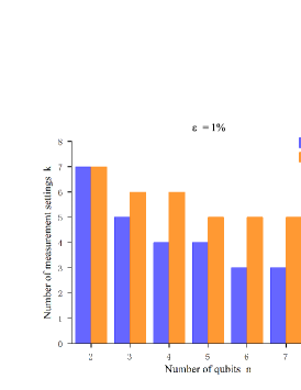
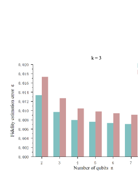
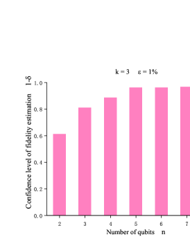
Figure 3: The performance of this method for fidelity estimation with neural networks varies with the number of qubits in the quantum state. (a) The number of measurement settings $k$ decreases as the number of qubits $n$ increases when $\epsilon=1\%$ and $1-\delta=95\%$ (or 99%). (b) The fidelity estimation error $\epsilon$ decreases as the number of qubits $n$ increases when $k=3$ and $1-\delta=95\%$ (or 99%). (c) The confidence level $1-\delta$ of the fidelity estimation grows with the increase of the number of qubits $n$ when $k=3$ and $\epsilon=1\%$. We note that the fidelity of the quantum state to be estimated here is in the range of 0.95 to 1.

Now we look at how to use a neural network model for a specific problem–to determine whether the fidelity of the input quantum states $|\psi_{1}\rangle$ and $|\psi_{2}\rangle$ 70data with respect to $|\psi_{0}\rangle$ exceeds 96%. Here we choose the confidence level $1-\delta$ to be 95%. For $|\psi_{1}\rangle$, we choose the top three Pauli operators in the absolute value of the expectation value for measurement, and input the measurement results into the neural network model with $k=3$, and obtain a fidelity prediction of $(97\pm 1)\%$, which indicates the fidelity of $|\psi_{1}\rangle$ exceeds 96%. For $|\psi_{2}\rangle$, repeating the above operations, the fidelity result obtained is $(95\pm 1.22)\%$, which cannot indicate whether the fidelity of $|\psi_{1}\rangle$ exceeds 96% for now. Then the Pauli operators with the fourth largest absolute value of expectation value are measured, and the measurement result was input into the $k=4$ neural network model together with the measurement results of the first three Pauli operators, and the fidelity prediction result obtained is $(94.78\pm 1)\%$, indicating that the fidelity of $|\psi_{2}\rangle$ does not exceed 96%.

Figure 3 shows how the performance of our method for fidelity estimation with neural networks varies with the number of qubits in the quantum state. In our scheme, in addition to the number of qubits $n$, there are three other parameters, which are the number of measurement settings $k$, the fidelity estimation error $\epsilon$, and the confidence level $1-\delta$ of the fidelity estimation. Figure (3a) shows that the number of measurement settings $k$ decreases as the number of qubits $n$ increases when $\epsilon=1\%$ and $1-\delta=95\%$ (or 99%). Figure (3b) shows that the fidelity estimation error $\epsilon$ decreases as the number of qubits $n$ increases when $k=3$ and $1-\delta=95\%$ (or 99%). Figure (3c) shows that the confidence level $1-\delta$ of the fidelity estimation grows with the increase of the number of qubits $n$ when $k=3$ and $\epsilon=1\%$. It can be seen from Fig. 3 that the performance of our method for estimating the fidelity of quantum states using neural networks is getting better as the number of qubits increases. This looks a bit counterintuitive, and we try to give an explanation for this phenomenon below.

From Eq. (3), the fidelity can be rewritten as

$$\begin{split}F(\rho_{0},\rho)&=\sqrt{\frac{1}{2^{n}}\sum\limits_{j=0}^{4^{n}-1}\beta_{j}a_{j}}\\ &=\sqrt{\sum\limits_{j=0}^{4^{n}-1}P_{j}\gamma_{j}},\end{split}$$ (4)

where $\gamma_{j}=\beta_{j}/a_{j}$, $P_{j}={a_{j}}^{2}/{2^{n}}$ and $\sum_{j=0}^{4^{n}-1}P_{j}=1$. It can be seen that the fidelity $F$ is equal to the square root of the weighted average of $\gamma_{j}$ in which $j$ ranges from 0 to $4^{n}-1$. For an ideal quantum state with unity fidelity, all $\gamma_{j}$ will have a value of 1; for a nonideal quantum state, these $4^{n}$ $\gamma_{j}$ will deviate from the value of 1. In the nonadversarial case, the deviation of $\gamma_{j}$ with respect to 1 will be general and random over all Pauli operators, and not concentrated on a few specific Pauli operators. Therefore, a fraction of $\gamma_{j}$ can be selected for measurement to estimate the overall deviation of $\gamma_{j}$ with respect to 1 and, thus, achieve the fidelity estimation. The larger the number of selected $\gamma_{j}$ (this number is defined as $l$), the smaller the error in the fidelity estimation. When $n$ is large, $l$ does not need to increase continuously to provide a good estimate of the fidelity 21Steven . As a visual example, for the United States presidential election with 260 million voters, the sample size of the poll only needs to be around 1000 69US .

With a fixed value of $l$, the number of required measurement settings $k$ decreases as the number of qubits $n$ increases. This is because, for each measurement setting for an $n$-qubit quantum state, $2^{n}$ possible outcomes will be produced, and using them the $\gamma_{j}$ corresponding to $2^{n}-1$ nontrivial Pauli operators can be calculated. For example, for the measurement results of one measurement setting for a three-qubit quantum state, the $\gamma_{j}$ corresponding to seven nontrivial Pauli operators can be calculated, while for the measurement results of one measurement setting for a six-qubit quantum state, the $\gamma_{j}$ corresponding to 63 nontrivial Pauli operators can be calculated. Thus, the number of measurement settings required to obtain $l$ $\gamma_{j}$ for a six-qubit state is less than that for a three-qubit state–this qualitatively explains why the performance of our method for estimating the fidelity of quantum states using neural networks is getting better as the number of qubits $n$ increases.

In the following, we compare our machine-learning-based fidelity estimation method with the other three methods QST, QSV and DFE, pointing out their respective advantages, disadvantages, and applicability. The advantage of QST is that it can characterize a completely unknown quantum state and reconstruct its density matrix to obtain all the information, while the other three methods can only evaluate the fidelity of the input quantum state with respect to a specific target quantum state. Its drawback is that the resources consumed grow exponentially with the size of the system. The advantage of QSV is that it can evaluate the fidelity of a quantum state with minimal resources, while its disadvantage is that it is currently only applicable to special quantum states such as stabilizer states and not to the case where the target quantum state is a multiqubit arbitrary pure quantum state. The advantage of DFE is that it is applicable to the case where the target quantum state is an arbitrary pure quantum state, and its disadvantage is that the selection of the measurement settings requires several rounds of random switching and the total number of measurement settings is relatively large. The advantage of our method is that it is not only applicable to the case where the target quantum state is an arbitrary pure quantum state, but also requires only a small number of measurement settings, and the number of required measurement settings does not increase with the size of the system. For example, for a seven-qubit arbitrary quantum state, our method only needs to switch the measurement settings three times to achieve a fidelity estimation within 0.01 error with $95\%$ confidence level, while to achieve the same result, QST needs to switch the measurement device $3^{7}=2187$ times and DFE needs to switch the measurement device ${8/[0.01^{2}\times(1-95\%)]}=1.6\times 10^{6}$ times. Note that QSV cannot evaluate the fidelity of an arbitrary seven-qubit quantum state. The disadvantage of our method is that it has an upper limit on the fidelity estimation accuracy, which is not suitable for situations requiring extremely high fidelity estimation accuracy. In summary, each of the four methods has its own advantages and disadvantages, which are complementary to each other and each is suitable for different application scenarios. Our method is most suitable for evaluating whether the fidelity of a quantum state exceeds a specific value with respect to an $n$-qubit arbitrary pure quantum state.

To summarize, we present, in this Letter, a method for predicting the fidelity of quantum states using neural network models. Compared with previous methods for quantum state fidelity estimation, our method uses fewer measurement settings and works for arbitrary quantum states. Here our method is applicable to nonadversarial scenarios. It has the potential to be used in a wide variety of local quantum information applications, such as quantum computation, quantum simulation, and quantum metrology. A future research direction is to design machine-learning-based quantum state fidelity estimation schemes in adversarial scenarios.

This work was supported by the National Key Research and Development Program (Grants No. 2017YFA0305200 and No. 2016YFA0301700), the Key Research and Development Program of Guangdong Province of China (Grants No. 2018B030329001 and No. 2018B030325001), the National Natural Science Foundation of China (Grant No. 61974168). X. Zhou acknowledges support from the National Young 1000 Talents Plan. W. Luo acknowledges support from the National Natural Science Foundation of China (Grant No. 61877029). X. Zhang acknowledges support from the National Natural Science Foundation of China (Grant No. 62005321). S. Pang acknowledges support from the National Natural Science Foundation of China (Grant No. 12075323).

X. Zhang and M. Luo contributed equally to this work.

Supplementary materials for “Direct Fidelity Estimation of Quantum States using Machine Learning”

In this supplementary material, we discuss more results. Sec.(I) describes the basic structure of artificial neural networks (ANNs) and our artificial neural network. Sec.(II) gives the method to generate quantum states with specified fidelity. It also analyzes the uniformity of pure state fidelity, mixed state fidelity The purity distribution of mixed states, the generality of our method, and Poisson noise are also presented here. The method for selecting the Pauli operators is given in Sec.(III). Sec.(IV) analyzes the accuracy of the quantum state fidelity estimation. Sec.(V) gives the verification accuracy of the neural network. Sec.(VI) presents a practical application of our neural network. Sec.(VII), we discuss the scalability of the neuron number.

I The structure of ANNs and our ANN

The basic structure of ANNs

ANNs consists of an input layer, hidden layers and an output layer (See Fig.1). The input layer consists of $k\times 2^{n}$ neurons corresponding to the probability of each outcome, in which $n$ represents the number of qubits and $k$ represents the number of Pauli combinations. We set the inputs $\bf{x_{0}}$ and the intermediate vector $\bf{x_{1}}$ in the hidden layer generated by the non-linear relation

$$\bf{x_{1}}=\sigma_{RL}(W_{1}\bf{x_{0}}+\bf{\omega_{1}}),$$ (5)

where $\sigma_{RL}$ is the ReLU function for each neuron in the hidden layer, defined as $\sigma_{RL}(z_{i})=max(z_{i},0)(i=1,2,3,...)$. The matrix $\bf{W_{1}}$ is the initialized weight and the vector $\bf{\omega_{1}}$ is the bias between the input layer and the hidden layer. The optimal output vector denoted as $\bf{x_{2}}$ is generated using the function

$$\bf{x_{2}}=\sigma_{s}(W_{2}\bf{x_{1}}+\bf{\omega_{2}}),$$ (6)

where $\sigma_{s}$ is the Softmax function defined by $\sigma(z_{i})=\frac{e^{z_{i}}}{\sum_{k=1}^{122}e^{z_{k}}}(i=1,...,122)$. The matrix $\bf{W_{2}}$ is the initialized weight between the hidden layer and the output layer, while the vector $\bf{\omega_{2}}$ is the bias. The loss function is categorical cross-entropy and is written as $-\frac{1}{n}[y_{s}loga_{s}+(1-y_{s})log(1-a_{s})]$. The subscript $s$ denotes the sequence number of the training sample, and the notation $y$ represents the labels defined by the criterion, $a$ means the output labels of the ANN and $n$ is the training set number, respectively. During the machine learning process, $W_{1}$, $\omega_{1}$, $W_{2}$, $\omega_{2}$ are continuously optimized until the confidence level reaches saturation, and then the training is stopped.

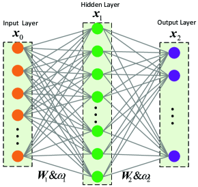
Figure 4: (Color online) Artificial neural networks with hidden layers. The objective of machine learning is to optimize $\sigma_{s}(\bf{W_{2}}\sigma_{RL}(\bf{W_{1}}\bf{x_{0}}+\bf{\omega_{1}})+\bf{\omega_{2}})$, where $\sigma_{RL}$ is ReLU function and $\sigma_{s}(z)_{i}=\frac{e^{z_{i}}}{\sum_{k=1}^{k}e^{z_{k}}}$ $(i=1,2,...,K)$ is softmax function. The input data $\bf{x_{0}}=\{a_{1},a_{2},\ldots,a_{k}\}$ are the measurements of Pauli operators. Matrix $\bf{W_{1}}$ and the vector $\bf{\omega_{1}}$ are initialized uniformly and optimized during the learning process. The number of neurons in the hidden layer can be varied for optimal performance. The output data $\bf{x_{2}}$ are the predicted fidelity.

The ANN for fidelity estimation

We use four 2080Ti GPUs. We choose the optimizer that has the best performance in our task among almost all the built-in optimizers in TensorFlow: NadamOptimizer (adaptive moment estimation). This neural network contains 122 labels, using 1,952,000 data for training and 488,000 data for validation, i.e. each label contains 16,000 training data and 4,000 validation data. By tuning the batch size of inputs, the number of neurons, and the number of training rounds, the performance of the neural network is continuously optimized. Eventually, the parameters required for training this neural network from two-qubit to seven-qubit quantum states are shown in Table S1 and Table S2. Hid-neu represents the number of the hidden neurons.

Table S1. Parameters of the neural network with $k\times[\frac{(n^{4}-2n^{3}+11n^{2}+14n)}{24}+1]$
expected values of non-trivial Pauli operators as the neuron inputs.
four-qubit states				five-qubit states
state	epoch	Batch size	Hid-neu	state	epoch	Batch size	Hid-neu
$|\varphi_{4}\rangle$	400	8192	2000	$|\varphi_{5}\rangle$	500	16384	700-300
			3000				900-300
			5000				1000-300
six-qubit states
state	epoch	Batch size	Hid-neu
$|\varphi_{6}\rangle$	500	16384	500-300
			700-300
			900-300

Table S2. Parameters of the neural network with all measurement
outcome probabilities as neuron inputs
two-qubit states				three-qubit states
state	epoch	Batch size	Hid-neu	state	epoch	Batch size	Hid-neu
Bell	200	2048	1000	GHZ	400	4096	1000
$W$			2000	W			2000
$|\varphi_{2}\rangle$			3000	$|\varphi_{3}\rangle$			3000
four-qubit states				five-qubit states
state	epoch	Batch size	Hid-neu	state	epoch	Batch size	Hid-neu
Cluster	400	8192		Cluster	200	16384
W			2000	C-ring			500-500
GHZ			3000	Dicke			1000-1000
Dicke			5000	GHZ			1500-1500
$|\varphi_{4}\rangle$				W
six-qubit states				$|\varphi_{5}\rangle$
state	epoch	Batch size	Hid-neu	seven-qubit states
$C_{23}$	500	16384		state	epoch	Batch size	Hid-neu
Dicke			500-500	$|\varphi_{7}\rangle$	500	16384
GHZ			1000-1000				800-400
W			1500-1500				900-400
$|\varphi_{8}\rangle$							1000-400
eight-qubit states
state	epoch	Batch size	Hid-neu
$|\varphi_{8}\rangle$	500	16384	700-400
			1000-400
			2000-500

Next, we show the specific forms of the special number states that appear in Table S2 (See Fig.2). Moreover, $|\varphi_{2}\rangle$, $|\varphi_{3}\rangle$, $|\varphi_{4}\rangle$, $|\varphi_{5}\rangle$, $|\varphi_{6}\rangle$, $|\varphi_{7}\rangle$ and $|\varphi_{8}\rangle$ are general quantum states 5states . The two-qubit Bell state and the W state are

$$\begin{array}[]{l}\displaystyle|\phi^{+}\rangle_{Bell}=\frac{1}{\sqrt{2}}(|00\rangle+|11\rangle),\\ \displaystyle|W\rangle=\frac{1}{\sqrt{3}}(|00\rangle+|01\rangle+|10\rangle).\end{array}$$ (9)

The three-qubit GHZ state and the W state are

$$\begin{array}[]{l}\displaystyle|GHZ\rangle=\frac{1}{\sqrt{2}}(|000\rangle+|111\rangle),\\ \displaystyle|W\rangle=\frac{1}{\sqrt{3}}(|001\rangle+|010\rangle+|100\rangle).\end{array}$$ (12)

The four-qubit Cluster state, the Dicke state, the GHZ state and the W state are

$$\begin{array}[]{l}\displaystyle|Cluster_{4}\rangle=\frac{1}{2}(|0000\rangle+|0011\rangle+|1100\rangle-|1111\rangle),\\ \displaystyle|Dicke_{4}^{2}\rangle=\frac{1}{\sqrt{6}}(|0011\rangle+|0110\rangle+|0101\rangle+|1010\rangle\\ \displaystyle\qquad\qquad\qquad+|1001\rangle+|1100\rangle),\\ \displaystyle|GHZ\rangle=\frac{1}{\sqrt{2}}(|0000\rangle+|1111\rangle),\\ \displaystyle|W\rangle=\frac{1}{2}(|0001\rangle+|0010\rangle+|0100\rangle+|1000\rangle).\end{array}$$ (18)

The five-qubit Cluster state, the C-ring state, the Dicke state, the GHZ state and the W state are

$$\begin{array}[]{l}\displaystyle\qquad|Cluster_{5}\rangle=\frac{1}{2}(|+0+0+\rangle+|+0-1-\rangle\\ \displaystyle\qquad\qquad\qquad+|-1-0+\rangle+|-1+1-\rangle),\\ \displaystyle\qquad|C\text{-}ring_{5}\rangle=\frac{1}{2\sqrt{2}}(|+0+00\rangle+|-0+01\rangle\\ \displaystyle\qquad\qquad\qquad+|+0-10\rangle-|-0-11\rangle+|-1-00\rangle\\ \displaystyle\qquad\qquad\qquad+|+1-01\rangle+|-1+10\rangle-|+1+11\rangle),\\ \displaystyle\qquad|Dicke_{5}^{2}\rangle=\frac{1}{\sqrt{10}}(|11000\rangle)+|10100\rangle+|01100\rangle\\ \displaystyle\qquad\qquad\qquad+|01010\rangle+|00110\rangle+|00101\rangle+|00011\rangle\\ \displaystyle\qquad\qquad\qquad+|10010\rangle+|10001\rangle+|01001\rangle),\\ \displaystyle\qquad|GHZ\rangle=\frac{1}{\sqrt{2}}(|00000\rangle+|11111\rangle),\\ \displaystyle\qquad|W\rangle=\frac{1}{\sqrt{5}}(|10000\rangle+|01000\rangle+|00100\rangle\\ \displaystyle\qquad\qquad\qquad+|00010\rangle+|00001\rangle).\end{array}$$ (30)

The six-qubit Cluster state, the Dicke state, the GHZ state and the W state are

$$\begin{array}[]{l}\displaystyle\qquad|C23\rangle=\frac{1}{2}(|+0++0+\rangle+|+0+-1-\rangle\\ \displaystyle\qquad\qquad\qquad+|-1-+0+\rangle-|-1--1-\rangle),\\ \displaystyle\qquad|Dicke_{6}^{2}\rangle=\frac{1}{\sqrt{15}}(|000011\rangle+|000101\rangle+|001010\rangle\\ \displaystyle\qquad\qquad\qquad+|001100\rangle+|110000\rangle+|010100\rangle+|101000\rangle\\ \displaystyle\qquad\qquad\qquad+|001001\rangle+|010001\rangle+|100001\rangle+|100010\rangle\\ \displaystyle\qquad\qquad\qquad+|100100\rangle+|000110\rangle+|011000\rangle+|010010\rangle),\\ \displaystyle\qquad|GHZ\rangle=\frac{1}{\sqrt{2}}(|000000\rangle+|111111\rangle),\\ \displaystyle\qquad|W\rangle=\frac{1}{\sqrt{6}}(|000001\rangle+|000010\rangle+|000100\rangle\\ \displaystyle\qquad\qquad+|010000\rangle+|100000\rangle.\end{array}$$ (40)

II Generation and analysis of quantum states

A. Generation of quantum pure states with specified fidelity

Preparing quantum states has an important role in realizing quantum information and quantum computing, but often the imperfection of devices and the influence of noise result in obtaining quantum states that are all mixed states. Here, we use neural network techniques to evaluate whether the fidelity between this quantum state and the ideal state satisfies the requirements. Our neural network inputs are derived from mixed states with specified fidelity. We first introduce the method for generating a pure state.

Step 1. Generating an arbitrary pure state
In Mathematics, we create a pure state of arbitrary dimension with the help of the function RandomKet(D) 40Miszczak . Specifically, The RandomKet(D) function calls RandomSimplex(D) and Randomreal(D) to generate a D-dimensional arbitrary pure state. The Mathematic code of generating an arbitrary pure state is shown below.

⬇

RandomSimplex[d_]:=Block[{r,r1,r2},

r=Sort[Table[RandomReal[{0,1}], {i,1,d-1}]];

r1=Append[r,1];

r2=Prepend[r,0]; r1-r2

];

RandomKet[n_]:=Block[{p, ph},

p=Sqrt[RandomSimplex[n]];

ph=Exp[I RandomReal[{0,2\[Pi]},n-1]];

ph=Prepend[ph,1];

p*ph

];

Step 2. Generation of a pure state with specified fidelity corresponding to the state $|0\rangle^{\otimes n}$
An arbitrary pure state can be expanded as

$$|\varphi\rangle=\sum_{i=0}^{2^{n}-1}\alpha_{i}|i\rangle,$$ (41)

where $|i\rangle$ $(i=0,1,...,2^{n}-1)$ is basis vector of calculations. For convenience, we rewrite Eq.(9) as follows.

$$|\varphi\rangle=f|0\rangle^{\otimes n}+\sum_{i=1}^{2^{n}-1}\alpha_{i}|i\rangle=f|0\rangle+\sqrt{1-f^{2}}|\phi\rangle^{2^{n}-1},$$ (42)

where $\alpha_{0}=f$. The state $|\phi\rangle^{2^{n}-1}$ is a $(2^{n}-1)$ dimensional arbitrary pure state. Therefore, the fidelity $f$ between $|0\rangle^{\otimes n}$ and $|\varphi\rangle$ is given as

$$f=F(|0\rangle^{\otimes n},|\varphi\rangle)=|\langle 0|^{\otimes n}|\varphi\rangle|$$ (43)

Hence, we can generate an $n$-qubit pure state dataset with the target state $|0\rangle^{\otimes n}$ using Matlab.

Step 3. Generation of a pure state with a specified fidelity corresponding to an arbitrary pure state
For convenience, we set $|\textbf{0}\rangle=|0\rangle^{\otimes n}$. Then we rewrite the Eq.(11) as follows.

$$f=F(|\bf{0}\rangle,\sigma)=\sqrt{\langle\bf{0}|\sigma|\bf{0}\rangle},$$ (44)

where $\sigma$ can be viewed as a state in the dataset $S$ with a target state $|\bf{0}\rangle$. If we choose a new target pure state $\rho$, there is a unitary matrix transformation $U$ from $|\bf{0}\rangle\langle\bf{0}|$ to $\rho$. This unitary $U$ can be calculated by the code Findunitary.m. As soon as such unitary is found 4Cramer ; 52Tacchino , the relative state of $\sigma$ is directly obtained as

$$\sigma^{\prime}=U\sigma U^{\dagger},$$ (45)

where the state $\sigma^{\prime}$ belongs to the database $S^{\prime}$ of the target state $\rho$. The fidelity $f^{\prime}$ between the target state $\rho$ and the state $\sigma^{\prime}$ can be calculated, that is,

$$f^{\prime}=F(\rho,\sigma^{\prime})=\sqrt{tr(\rho,\sigma^{\prime})}=\sqrt{\langle\bf{0}|U^{\dagger}\sigma^{\prime}U|\bf{0}\rangle}=\sqrt{\langle\bf{0}|\sigma|\bf{0}\rangle}=f.$$ (46)

Step 4. Projective measurements
Each measurement setting $k$ is characterized by $W_{k}$, and each specific result $p(k_{j})$ is associated with a projection operator

$$P_{k_{j}}=|v_{k_{j}}\rangle\langle v_{k_{j}}|,\quad j=1,2,...,2^{n},$$ (47)

where $|v_{k_{j}}\rangle$ is the $j_{th}$ eigenvector of the $W_{k}$, $p(k_{j})$ is equal to $tr(\rho P_{k_{j}})$.

B. Generation of quantum mixed states with specified fidelity

Here we give the method for generating mixed states with specified fidelity. In a Ginibre matrix $G$, each element is the standard complex normal distribution $CN(0,1)$. The random density matrix of mixed states can be written as

$$\rho=\frac{GG^{\dagger}}{tr(GG^{\dagger})}.$$ (48)

Inspired by the Ginibre matrix $G$, we propose a method to prepare specified fidelity states with the target state $|\bf{0}\rangle$, i.e., the density matrix of desired N-qubit mixed state is

$$\rho_{n}=\frac{\mathbb{G}_{n}\mathbb{G}_{n}^{\dagger}}{tr(\mathbb{G}_{n}\mathbb{G}_{n}^{\dagger})}.$$ (49)

where the matrix $\mathbb{G}_{n}$ can be expressed as

$$\mathbb{G}_{n}=\left(\sqrt{m_{1}}\left(\begin{array}[]{c}x_{1}e^{-2\pi i*rand_{11}}\\ \sqrt{1-x_{1}^{2}}e^{-2\pi i*rand_{12}}|\varphi_{1}\rangle\\ \end{array}\right),...,\sqrt{m_{n}}\left(\begin{array}[]{c}x_{n}e^{-2\pi i*rand_{n1}}\\ \sqrt{1-x_{n}^{2}}e^{-2\pi i*rand_{n2}}|\varphi_{n}\rangle\\ \end{array}\right)\right)$$ (54)

The notations $rand_{b1}$ and $rand_{b2}$ ($b=1,2,...,n$) represent random numbers. The set $\{|\varphi_{1}\rangle,...,|\varphi_{n}\rangle\}$ is a collection of $2^{n}-1$ dimensional pure states produced by the function RandomKet. $\{m_{1},..,m_{n}\}$ is a set of real numbers of $2^{N}$ dimension normalized standard normal distribution. $\{x_{1},...,x_{n}\}$ is a set of undefined real numbers that are closely related to the expected fidelity.

The steps for preparing the mixed state are similar to those for preparing the pure state. As can be seen from Eq.(18), the density matrix of a mixed state with specified fidelity needs to determine the values of $\{m_{1},...,m_{n}\}$ and $\{x_{1},...,x_{n}\}$, where the former is generated randomly using the Matlab code and the latter is determined according to the corresponding constraints.

An example.–For a two-qubit state, suppose the desired fidelity is $f_{0}$ for the target state $|00\rangle$. The values $\{x_{1},x_{2},x_{3},x_{4}\}$ in the matrix $\mathbb{G}_{n}$ can be determined from Eqs. (18-21) using Matlab. The value range of $x_{1}$ can first be determined in Eq.(18) by the given fidelity $f_{0}$. When we fix the $x_{1}$ randomly and uniformly, the value range of $x_{2}$ can also be determined in Eq.(19). Then we fix the $x_{2}$ randomly and uniformly, and the value range of $x_{3}$ can also be defined in Eq.(20). Once the value of $x_{3}$ is fixed randomly and uniformly, the value of $x_{4}$ is also fixed in Eq.(21). Therefore, we obtain the matrix $\mathbb{G}_{n}$.

$$x_{1}\in[min\{max(\frac{f_{0}^{2}-\sum\limits_{i=2}^{4}m_{i}}{m_{1}},0),1\},min\{max(\frac{f_{0}^{2}}{m_{1}},0),1\}]$$ (55)

$$x_{2}\in[min\{max(\frac{f_{0}^{2}-m_{1}x_{1}^{2}\sum_{i=3}^{4}m_{i}}{m_{2}},0),1\},min\{max(\frac{f_{0}^{2}-m_{1}x_{1}^{2}}{m_{1}},0),1\}],$$ (56)

$$x_{3}\in[min\{max(\frac{f_{0}^{2}-\sum\limits_{i=1}^{2}m_{i}x_{i}^{2}-m_{4}}{m_{2}},0),1\},min\{max(\frac{f_{0}^{2}-\sum\limits_{i=1}^{2}m_{i}x_{i}^{2}}{m_{2}},0),1\}],$$ (57)

$$x_{4}=\frac{f_{0}^{2}-\sum\limits_{i=1}^{3}m_{i}x_{i}^{2}}{m_{4}}.$$ (58)

C. Uniformity analysis of pure state fidelity

We use a computer to generate 500 single-qubit pure states. The fidelity between each of 500 pure states and the state $|0\rangle$ is $\sqrt{0.5}$. We also give a geometric representation of the Bloch ball in Fig.3(a). It is obvious that the distribution of 500 states is uniform.

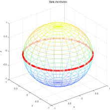
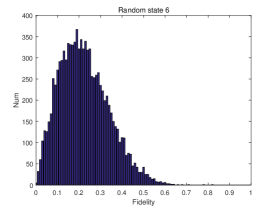
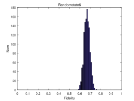
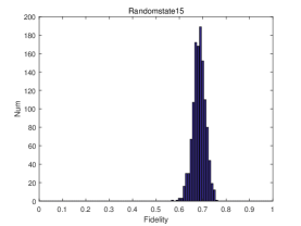
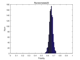
Figure 6: (Color Online) (a) Distribution of 500 single-qubit states in the Bloch ball; (b)The distribution of 10,000 four-qubit pure states containing state 6 and state 20; (c) The distribution of 1,220 four-qubit mixed states including state 6, state 15 and state 20.

In addition, we verify the uniformity of four-qubit pure states fidelities. We generate 10,000 four-qubit pure states, in which the fidelity between each of these states and the state $|0000\rangle$ is 0.25. We select 20 states out of the 10,000 states, and the fidelity between each selected state and 9,999 other states can be calculated. We get 20 similar distributions, including the distribution of random state 6 and the distribution of the random state 20 in Fig.3(b). We conclude that the distribution of 10,000 states is uniform.

D. Uniformity analysis of mixed state fidelity

Here, we verify the uniformity of four-qubit mixed states datasets in Fig.3(c). A total of 1,220 states are generated, in which the fidelity between 1,220 states and the state $|0000\rangle$ is 0.25. We also select 20 states out of 1,220 states. The fidelity, between each selected state and the other 1,219 states, can be calculated. We get 20 similar distribution patterns, including the distribution of random state 6, random state 15 and the distribution of random state 20 in Fig.3(c). We found that the distribution of the 1,220 states is uniform.

E. Distribution of different purities of mixed states

The purity of a quantum state $\rho$ is defined as $tr(\rho^{2})$, where $tr(\rho^{2})=1$ means that this quantum state is pure and vice versa is a mixed state. Figure 4 shows the distribution of purity for 1,220 four-qubit mixed states, in which $m_{1}$ can control the purity of quantum states. In Fig.4(a-b) the fidelity $f_{0}$ between the prepared state and $|0000\rangle$ is 0.25, and the fidelity $f_{1}$ is 0.8 in Fig.4(c-d). The controller $m_{1}$ is equal to 1, 0.9, 0.6, 0.2 or 0.01. Moveover, $m_{1}$ can also be a uniform distribution $U(0,1)$. The analysis here demonstrates how to control the purity of the prepared states.

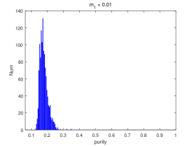
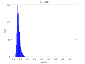
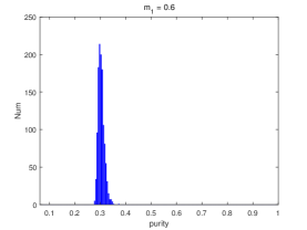
(a) $f_{0}$=0.25

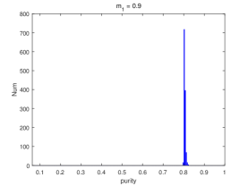
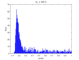
(b) $f_{0}$=0.25

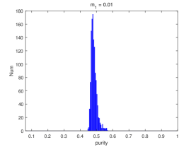
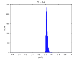
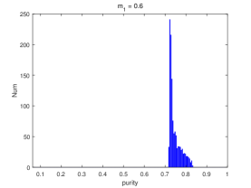
(c) $f_{0}$=0.8

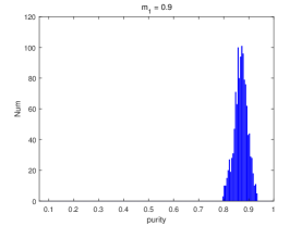
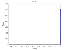
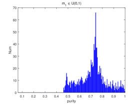
(d) $f_{0}$=0.8

Figure 7: (Color Online) Comparison of mixed-state distributions for different purity, where $m_{1}=1,0.9,0.6,0.2,0.01,U(0,1)$. The specified quantum states fidelities are 0.25 and 0.8 respectively.

Here, we discuss nine datasets in Table S3 for the four-qubit general state $|\varphi_{4}\rangle$, in which eight datasets belong to mixed states and the rest one to pure states. In eight mixed datasets, the purity distribution of $m_{1}$ is changed for seven datasets and the remaining one does not change the distribution of $m_{1}$.

Table S3. Nine distributions of $m_{1}$
ANN models	datasets	$m_{1}$ distribution
A	1	$m_{1}=1-rand*rand$
B	2	$m_{1}=1-\sqrt{rand}*rand$
C	3	$m_{1}$ belongs to a uniform distribution $U(0,1)$
D	4	$m_{1}$ belongs to a random standard normal distribution $N(0,1)$
E	5	Pure states
F	6	$m_{1}=1-rand*rand*rand$
G	7	$m_{1}=1-rand*rand*rand*rand$
H	8	$m_{1}=1-rand^{3}$
I	9	$m_{1}=1-rand*rand^{3}$

By comparing the distribution from Table S4, it can be seen that the distribution $m_{1}=1-rand^{3}$ is better than others because this distribution is effective for mixed states and pure states. It is worth note that the states in this distribution $m_{1}=1-rand^{3}$ are closer to pure states than those in other distributions. Here we only show the validation results of $k=3,4,5$ of nine ANN models for nine datasets because from these results can draw the conclusion we give.

Table S4. Accuracy of nine ANN models for nine datasets
datasets	1	2	3	4	5	6	7	8	9
	A
3	79.78%	80.57%	81.11%	77.19%	72.60%	78.09%	76.41%	78.32%	77.12%
4	86.99%	87.33%	87.42%	83.37%	82.62%	86.34%	85.45%	86.10%	85.63%
5	89.82%	90.26%	89.94%	85.96%	87.26%	90.01%	89.48%	89.43%	89.59%
	B
3	78.84%	80.24%	81.21%	77.61%	67.65%	76.47%	73.82%	77.04%	74.98%
4	86.34%	87.03%	87.36%	83.75%	78.13%	84.70%	82.97%	84.84%	83.57%
5	89.58%	90%	89.70%	86.49%	83.56%	88.89%	87.93%	88.65%	88.17%
	C
3	77.53%	79.07%	80.29%	77.44%	66.83%	74.62%	71.98%	75.59%	75.59%
4	85.36%	86.32%	87.11%	83.61%	76.39%	83.14%	81.01%	83.69%	83.69%
5	88.67%	89.38%	89.72%	86.24%	81.36%	87.02%	85.34%	87.29%	87.29%
	D
3	75.29%	77.62%	79.37%	76.67%	59.93%	70.81%	67.10%	72.51%	69.18%
4	82.65%	84.39%	85.60%	82.80%	69.73%	79.13%	76.01%	80.27%	77.61%
5	85.72%	86.91%	87.74%	85.26%	76.09%	83.25%	80.90%	83.89%	82.05%
	E
3	22.93%	15.73%	11.10%	10.96%	85.05%	38.62%	54.07%	34.86%	46.63%
4	26.66%	18.21%	12.64%	12.63%	91.83%	44.57%	61.47%	39.29%	52.52%
5	27.60%	18.59%	12.49%	12.24%	95.07%	46.41%	64.04%	40.60%	54.55%
	F
3	80.02%	80.13%	80.18%	76.15%	75.52%	79.66%	78.62%	79.19%	78.86%
4	87.47%	86.94%	86.49%	82.64%	85.10%	87.66%	87.48%	86.93%	87.10%
5	90.45%	90.24%	89.55%	85.58%	90.70%	91.27%	91.37%	90.46%	91.04%
	G
3	79.13%	78.84%	78.65%	74.30%	78.77%	79.58%	79.67%	78.96%	78.39%
4	86.63%	85.97%	85.35%	81.16%	86.86%	87.63%	88.16%	86.78%	87.17%
5	90.43%	89.57%	88.58%	84.44%	91.87%	91.67%	92.25%	90.50%	90.92%
	H
3	79.09%	79.51%	80.78%	76.93%	76.03%	78.37%	77.45%	78.65%	78%
4	87.26%	87.15%	86.80%	83.11%	84.64%	87.09%	86.27%	86.75%	86.58%
5	90.65%	90.32%	89.24%	85.77%	89.30%	90.94%	90.38%	90.28%	90.59%
	I
3	79.73%	79.88%	79.15%	75.84%	76.82%	79.62%	79.18%	79.33%	78.65%
4	86.82%	86.36%	86.39%	82.18%	86.92%	87.30%	87.53%	86.79%	87.39%
5	90.08%	89.46%	88.81%	85.18%	91.23%	91%	91.46%	90.26%	91.08%

F. Universality of our method

We will prove the universality of our methods for preparing quantum states. To better demonstrate this inference, we show three dataset classes with three six-qubit general target pure states $|\varphi_{6}^{1}\rangle,|\varphi_{6}^{2}\rangle,|\varphi_{6}^{3}\rangle$, respectively. By analyzing the results from Table S5, we conclude that our method of preparing database is universal, corresponding to an arbitrary target pure state.

Table S5. Datasets comparison of three six-qubit general states
six-qubit (Hid-neu:700-300, precision with $\pm 1\%$)
	$|\varphi_{6}^{1}\rangle$	$|\varphi_{6}^{2}\rangle$	$|\varphi_{6}^{3}\rangle$
2	79.17%	77.76%	78.77%
3	86.89%	85.39%	88.03%
4	91.52%	90.56%	92.49%
5	94.09%	93.68%	94.48%
6	95.21%	95.19%	94.81%
7	97.10%	96.24%	97.15%

G. Poisson noise analysis

In an experiment, noise is inevitable. In our work, we assume that the noise follows the Poisson law. Using the random function in Matlab, we can obtain one value from the Poisson distribution with $NP$, in which $P$ is the basis measurements, and $NP$ is the ideal coincidence count.

We give a comparison of different number of samples for a four-qubit general state (See Fig.5). The noise model uses the number of samples of $N=$1,000, 4000, 7,000, 10,000, 10,0000 and 1,000,000. For comparison, we find that the noise model for the number of sample $N=$10,000 is appropriate. Therefore, these datasets are generated with the number of samples $N=$10,000 from two-qubit to seven-qubit states.

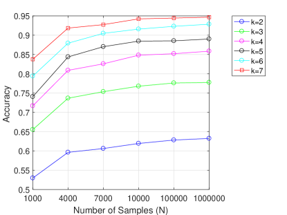
Figure 8: (Color online) Comparison of the accuracy of neural network models with different number of samples. Taking a four-qubit general state as an example, when $k=2,3,4,5,6,7$, the neural network models with the number of samples 1000, 4000, 7000, 10000, 100000, 100000 are generated respectively. The higher the number of Pauli operator measurement settings used, the higher the prediction accuracy is. The higher of the number of samples $N$ is, the higher the accuracy is.

III Selection of Pauli combinations

Let $W_{k}$ $(k=1,2,...,2^{2n})$ denotes all possible Pauli operators ($n$-fold tensor products of $I$, $X$, $Y$ and $Z$). Then $tr(\rho\sigma)$ can be rewritten in Ref.40Miszczak as follows.

$$tr(\rho\sigma)=\sum_{k}\frac{1}{d}\chi_{\rho}(k)\chi_{\sigma}(k),$$ (59)

where the characteristic function is defined as $\chi_{\rho}(k)=tr(\rho W_{k})$. For a target pure state $\rho$, we define the weight $Pr(k)$ corresponding to the Pauli operators $W_{k}$.

$$Pr(k)=[\chi_{\rho}(k)]^{2},$$ (60)

If we want to know the fidelity between a target pure state and an arbitrary state, we need to get $\chi_{\sigma}(k)$ in Eq.(23) related to the weight $Pr(k)\neq 0$. Obviously, the general state requires more Pauli combinations than a special state. Here we have chosen the $k$ Pauli operators with the largest absolute value of the expectation value of the desired quantum state.

Here we show the accuracy of the neural network for the Pauli operators with a large absolute value of expectation and for the Pauli operators with a small absolute value of expectation, respectively (See Table S6). Take the four-qubit cluster state and the general state as an example, the ANN model for the Pauli operator with a large absolute value of expectation can get more information than that for the Pauli operator with a small absolute value of expectation.

Table S6. Comparison of two types of weights
four-qubit states (Precision $\pm 1\%$)
	$|\varphi_{4}\rangle$(largest weight,	$|\varphi_{4}\rangle$(smallest weight,	Cluster (weight=1,	Cluster (weight=0,
	Hid-neu:5000)	Hid-neu:5000)	Hid-neu:3000)	Hid-neu:3000)
2	61.48%	56.35%	90.75%	67.99%
3	77.18%	69.43%	96.45%	81.98%
4	84.51%	77.79%	98.48%	91%
5	88.47%	83.70%	99.37%	96.18%
6	91.80%	90.76%	99.81%	97.34%
7	94.21%	92.83%	99.96%	97.67%

We then show the selected Pauli operators from two-qubit to eight-qubit states in Table S7.

Table S7. Pauli operators
two-qubit		three-qubit
states	Pauli operators	states	Pauli operators
Bell	XX;YZ;ZY;YY;ZX;XZ;XY	GHZ	ZZZ;XXX;XYY;YXY;YYX; YYY;XXZ
$W_{2}$	XX;YZ;ZY;XZ;YY;ZX;ZZ	W	ZZZ;ZXX;ZYY;XZX;XXZ;YZY;YYZ
$|\varphi_{2}\rangle$	XY;YX;ZZ;YZ;XX;ZY;YY;ZX;XZ	$|\varphi_{3}\rangle$	YYY;XXY;ZZY;XYZ;YXX;YXZ;YXY
four-qubit
Cluster	ZZXX;ZZYY;XXZZ;YYZZ;XYXY;XYYX;YXXY
Dicke	XXXX;YYYY;ZZZZ;XXZZ;ZZYY;ZZXX;YYZZ
GHZ	XXXX;YYYY;ZZZZ;XXYY;XYXY;YXYX;YYXX
W	ZZZZ;ZZXX;ZZYY;XXZZ;YYZZ;XZXZ;YZYZ
$|\varphi_{4}\rangle$	YXXZ;XYZX;ZZYY;YZXX;XYZY;YXZZ;ZZYX
five-qubit
Cluster	XZZXZ;ZYXYZ;ZXZZX;YXXXY;YYZZX;XZZYY;ZYXXY
C-ring	XXXXX;ZYXYZ;ZZYXY;XYZZY;YXYZZ;YZZYX;XZZYX
Dicke	ZZZZZ;XXXXZ;YYYZY;ZZZXX;ZYYYY;YZZYZ;XXXZX
GHZ	XXXXX;ZZZZZ;XYXXY;XYXYX;XYYXX;YXYYY;YYXYY
W	ZZZZZ;XXZZZ;XZZXZ;YYZZZ;YZZYZ;ZXZXZ;ZYZYZ
$|\varphi_{5}\rangle$	YYXZX;XZZYZ;ZYYYY;XZYXX;XXZZY;YZXXZ;ZYXZY
six-qubit
C23	XZXYXY;XZXYXY;ZXYZYZ;ZYZYXZ;YXYXZX;XZXZYY;ZYZZXY
Dicke	ZZZZZZ;XXZZZZ;ZZZZYY;ZZYYZZ;ZZXZZX;ZZZXXZ;YYZZZZ
GHZ	XXXXXX;YYYYYY;ZZZZZZ;XXXYYY;XYYYYX;YXYYXY;YYYYXX
W	ZZZZZZ;XZXZZZ;XZZZZX;YYZZZZ;YZZZYZ;ZXZXZZ;ZYZZYZ
$|\varphi_{6}\rangle$	XXYXYX;ZZXYZZ;YYZYXZ;ZZXZXY;ZXYXYY;ZYZZZX;YZZYZY
seven-qubit
$|\varphi_{7}\rangle$	XYZXXXX;ZZXZYYY;YXXYZZZ;ZYYZZZZ;XXZYYYX;YZXZXXY;ZYYXYZX
eight-qubit
$|\varphi_{8}\rangle$	XXXXXXXX;YYYYYYYY;ZZZZZZZZ;XYZXYZXY;YZXYZXYZ

IV Precision of fidelity estimation

Figure 6 presents some important information about the neural network with different number of labels. In Fig.6(a-c), in the case of a fixed number of labels, the higher the number of Pauli operator measurement settings used, the higher the prediction accuracy is. Meanwhile, the higher the fidelity of the predicted quantum states is, the higher the accuracy is. In Fig.6(d), the more quantum state fidelity intervals are divided, the higher the accuracy is. However, the accuracy of the neural network model with 234 labels is not much higher than that of the neural network model with 122 labels. Moreover, the higher the number of labels are, the more resources and time are consumed, so the neural network with 122 labels is selected as the most appropriate. The fidelity interval of the quantum state is respectively divided into 66 labels, 122 labels and 234 labels for the specific interval in Ref.67three .

V Accuracies of ANN models for N-qubit states

In Table S8, we show all the accuracies of the ANN models from two-qubit to seven-qubit states with the precision $\pm 1\%$.

Table S8. Accuracies of ANN models
	two-qubit (Hid-neu:2000)			three-qubit (Hid-neu:2000)
	Bell	$W_{2}$	$|\varphi_{2}\rangle$	GHZ	W	$|\varphi_{3}\rangle$
2	30.81%	46.65%	36.56%	34.65%	57.35%	54.22%
3	50.50%	64.87%	62.50%	62.55%	68.10%	68.38%
4	76.73%	78.68%	76.25%	70.40%	76.78%	80.10%
5	90.16%	92.21%	80.66%	77.75%	86.65%	89.49%
6	99.99%	93.90%	87.27%	81.23%	89.07%	92.72%
7	99.99%	99.99%	93.38%	87.73%	89.87%	95.38%
	four-qubit (Hid-neu:2000)
	Cluster	GHZ	W	Dicke	$|\varphi_{4}\rangle$
2	90.66%	78.19%	86.86%	91.56%	61.93%
3	96.47%	97.82%	89.25%	96.77%	76.77%
4	98.51%	98.53%	93.58%	99.41%	84.81%
5	99.40%	99.34%	95.53%	99.80%	88.45%
6	99.79%	99.74%	96.83%	99.97%	91.57%
7	99.96%	99.94%	97.92%	99.99%	94.22%
	five-qubit (Hid-neu:500-300)
	Cluster	C-ring	Dicke	GHZ	W	$|\varphi_{5}\rangle$
2	87.26%	79.87%	84.34%	92.28%	81.67%	70.40%
3	89.73%	82.96%	89.08%	93.15%	91.49%	81.75%
4	90.48%	84.52%	92.62%	93.89%	93.87%	88.14%
5	91.67%	85.16%	95.71%	95.85%	95.87%	93.16%
6	92.76%	86.19%	96.96%	96.62%	96.52%	95.92%
7	93.09%	86.89%	97.35%	97.23%	97.21%	96.44%
	six-qubit (Hid-neu:1500-1500)			seven-qubit (Hid-neu:1000-400)
	GHZ	C23	W	Dicke	$|\varphi_{6}\rangle$	$|\varphi_{7}\rangle$
2	98.28%	92.24%	92.91%	90.46%	79.17%	83.44%
3	99.04%	93.48%	94.86%	96.69%	86.89%	89.90%
4	99.42%	94.69%	97.8%	97.82%	91.52%	93.47%
5	99.64%	95.25%	98.24%	98.07%	94.09%	95.04%
6	99.79%	97.11%	98.79%	98.19%	95.21%	96.42%
7	99.87%	97.41%	99.22%	99.01%	97.10%	97.16%

VI Applications of our neural networks

How can we use a trained neural network to determine whether the fidelity of an input quantum state is higher than 96%. The fidelity of this quantum state is first predicted using a neural network with $k=2$. If the upper bound of the predicted fidelity range given does not exceed 96%, the neural network gives the prediction that determines that the fidelity of this state does not exceed 96%. If the lower bound of the predicted fidelity range is more than 96%, the neural network will give a prediction that the fidelity of this state is more than 96%. If the range of prediction fidelity is given including 96%, it is necessary to determine whether the prediction accuracy reaches $\pm 1\%$. If the prediction accuracy reaches $\pm 1\%$, the neural network determines that the fidelity of this state does not exceed 96%. If the prediction accuracy does not reach $\pm 1\%$, the neural network cannot determine that the fidelity of this state does not exceed 96%. Therefore, we continue the prediction with the $k=3$ neural network and repeat the above test process. Finally, the neural network can determine whether the fidelity of this state exceeds 96%.

VII Discussion on the scalability of the neuron number

In the main text, we discuss the case $M=2^{n}-1$, and in this supplementary section we discuss the case $M<2^{n}-1$. When $n$ is large, $2^{n}-1$ will be very large, and it is impossible and unnecessary for us to compute all expectation values of the $2^{n}-1$ non-trivial Pauli operators and take them as neuron inputs; we can select only some of them for neuron inputs. For example, we can select those Pauli operators that contain no more than three Identity operators. There are C(n,4)+C(n,3)+C(n,2)+C(n,1)+C(n,0) such Pauli operators, so $M$ will be set to $\frac{1}{24}(n^{4}-2n^{3}+11n^{2}+14n)+1$. If we set $k$ to $2n$, the number of input neurons $k\times M$ becomes $\frac{1}{12}(n^{5}-2n^{4}+11n^{3}+14n^{2})+2n$, only of the order of $n^{5}$ and does not increase exponentially with $n$. Figure 7 shows how the performance of our neural network fidelity estimation changes as $n$ increases from 4 to 6 for the case of $M=\frac{1}{24}(n^{4}-2n^{3}+11n^{2}+14n)+1$, $k=2n$ and $1-\delta=95\%$ (or 99%). We can see that in this case the error of fidelity estimation do not increase as $n$ increases.

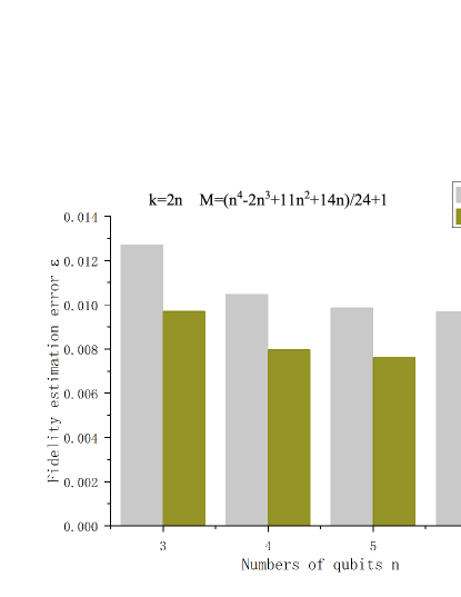
Figure 10: (Color Online) The performance of this method for fidelity estimation with neural networks varies with the number of qubits in the quantum state. The fidelity estimation error $\epsilon$ do not increase as the number of qubits $n$ increases for the case of $M=\frac{1}{24}(n^{4}-2n^{3}+11n^{2}+14n)+1$, $k=2n$ and $1-\delta=95\%$ (or 99%).

References

- (1) A. Chantasri, S.-S. Pang, T. Chalermpusitarak, and A. N. Jordan, Quantum state tomography with time-continuous measurements: Reconstruction with resource limitations, Quantum Stud 7, 23 (2020).
- (2) G. Toth, W. Wieczorek, D. Gross, R. Krischek, C. Schwemmer, and H. Weinfurter, Permutationally Invariant Quantum Tomography, Phys. Rev. Lett. 105, 250403 (2010).
- (3) M. Cramer, M. B. Plenio, S. T. Flammia, R. Somma, D. Gross, S. D. Bartlett, O. Landon-Cardinal, D. Poulin, and Y. Liu, Efficient quantum state tomography, Nat. Commun. 1, 149 (2010).
- (4) J. Renes, R. Blume-Kohout, A. Scott, and C. Caves, Symmetric informationally complete quantum measurements, J. Math. Phys.(N.Y.) 45, 2171 (2004).
- (5) D. Gross, Y. Liu, S. T. Flammia, S. Becker, and J. Eisert, Quantum State Tomography via Compressed Sensing, Phys. Rev. Lett. 105, 150401 (2010).
- (6) S. T. Flammia, D. Gross, Y. Liu, and J. Eisert, Quantum tomography via compressed sensing: Error bounds, sample complexity and efficient estimators, New J. Phys. 14, 095022 (2012).
- (7) A. Smith, C. A. RiofrÍo, B. E. Anderson, H. Sosa-Martinez, I. H. Deutsch, and P. S. Jessen, Quantum state tomography by continuous measurement and compressed sensing, Phys. Rev. A 87, 030102(R) (2013).
- (8) A. Kalev, R. L. Kosut, and I. H. Deutsch, Quantum tomography protocols with positivity are compressed sensing protocols, npj Quantum Inf. 1, 15018 (2015).
- (9) C. RiofrÍo, D. Gross, S. Flammia, T. Monz, D. Nigg, R. Blatt, and J. Eisert, Experimental quantum compressed sensing for a seven-qubit system, Nat. Commun. 8, 15305 (2017).
- (10) A. Kyrillidis, A. Kalev, D. Park, S. Bhojanapalli, C. Caramanis, and S. Sanghavi, Provable compressed sensing quantum state tomography via non-convex methods, npj Quantum Inf. 4, 36 (2018).
- (11) J. Shang, Z. Zhang, and H. K. Ng, Superfast maximum-likelihood reconstruction for quantum tomography, Phys. Rev. A 95, 062336 (2017).
- (12) G. Silva, S. Glancy, and H. Vasconcelos, Investigating bias in maximum-likelihood quantum-state tomography, Phys. Rev. A 95, 022107 (2017).
- (13) C. Oh, Y. Teo, and H. Jeong, Efficient Bayesian credible region certification for quantum-state tomography, Phys. Rev. A 100, 012345 (2019).
- (14) V. Siddhu, Maximum a probability estimates for quantum tomography, Phys. Rev. A 99, 012342 (2019).
- (15) X. Ma, T. Jackson, H. Zhou. J.-X. Chen, D.-W. Lu, M. D. Mazurek, K. A. G. Fisher, X.-H. Peng, D. Kribs, K. J. Resch, Z.-F. Ji, B. Zeng, and R. Laflamme, Pure-state tomography with the expectation value of pauli operators, Phys. Rev. A 93, 032140 (2016).
- (16) D. Martnez, M. SolÍ-Prosser, G. Cañas, O. Jiménez, A. Delgado, and G. Lima, Experimental quantum tomography assisted by multiply symmetric states in higher dimensions, Phys. Rev. A 99, 012336 (2019).
- (17) H. Sosa-Martinez, N. Lysne, C. Baldwin, A. Kalev, I. Deutsch, and P. Jessen, Experimental Study of Optimal Measurements for Quantum State Tomography, Phys. Rev. Lett. 119, 150401 (2017).
- (18) C.-Y. Lu. O. Gühne, W.-B. Gao, and J.-W. Pan, Toolbox for entanglement detection and fidelity estimation, Phys. Rev. A 76, 030305(R) (2007).
- (19) Y. Tokunaga, T. Yamamoto, M. Koashi, and N. Imoto, Fidelity estimation and entanglement verification for experimentally produced four-qubit cluster states, Phys. Rev. A 74, 020301(R) (2006).
- (20) S. T. Flammia and Y.-K. Liu, Direct Fidelity Estimation from Few Pauli Measurements, Phys. Rev. Lett. 106, 230501 (2011).
- (21) M. P. da Silva, O. Landon-Cardinal, and D. Poulin, Practical Characterization of Quantum Devices without Tomography, Phys. Rev. Lett. 107, 210404 (2011).
- (22) H.-J. Zhu and M. Hayashi, Optimal verification and fidelity estimation of maximally entangled states, Phys. Rev. A 99, 052346 (2019).
- (23) M. Cerezo, A. Poremba, L. Cincio, and P. J. Coles, Variational quantum fidelity estimation, Quantum 4, 1 (2020).
- (24) D. S. Rolando, J. Chiaverini, and D. J. Berkeland, Lower bounds for the fidelity of entangled-state preparation, Phys. Rev. A 74, 052302 (2006).
- (25) J. Wang, Z. Han, S. Wang, Z. Li, L. Mu, H. Fan, and L. Wang, Scalable quantum tomography with fidelity estimation, Phys. Rev. A 101, 032321 (2020).
- (26) D. Mahler, L. A. Rozema, A. Darabi, C. Ferrie, R. Blume-Kohouz, and A. Steinberg, Adaptive Quantum State Tomography Improves Accuracy Quadratically, Phys. Rev. Lett. 111, 183601 (2013).
- (27) Z.-H. Li, Y.-G. Han, and H.-J. Zhu, Efficient verification of bipartite pure states, Phys. Rev. A 100, 032316 (2019).
- (28) X.-D. Yu, J.-W. Shang, and O. Gühne, Optimal verification of general bipartite pure states, npj Quantum Inf. 5, 112 (2019).
- (29) H.-J. Zhu and M. Hayashi, Efficient Verification of Pure Quantum States in the Adversarial Scenario, Phys. Rev. Lett. 123,260504 (2019).
- (30) Y.-C. Liu, X.-D. Yu, J.-W. Shang, H.-J. Zhu, and X.-D. Zhang, Efficient Verification of Dicke States, Phys. Rev. Applied 12, 044020 (2019).
- (31) H.-J. Zhu and M. Hayashi, Efficient Verification of Hypergraph States, Phys. Rev. Applied. 12, 054047 (2019).
- (32) K. Wang and M. Hayashi, Optimal verification of two-qubit pure states, Phys. Rev. A 100, 032315 (2019).
- (33) H.-J. Zhu and M. Hayashi, General framework for verifying pure quantum states in the adversarial scenario, Phys. Rev. A 100, 062335 (2019).
- (34) Z.-H. Li, Y.-G. Han, and H.-J. Zhu, Optimal Verification of Greenberger-Horne-Zeilinger states, Phys. Rev. Applied 13,054002 (2020).
- (35) S. Pallister, N. Linden, and A. Montanaro, Optimal Verification of Entangled States with Local Measurements, Phys. Rev. Lett. 120, 170502 (2018).
- (36) W.-H. Zhang, C. Zhang, Z. Chen, X.-X. Peng, X.-Y. Xu, P. Yin, S. Yu, X.-J. Ye, Y.-J. Han, J.-S. Xu, G. Chen, C.-F. Li, and G.-C. Guo, Experimental optimal verification of entangled states using local measurements, Phys. Rev. Lett. 125, 030506 (2020).
- (37) X.-H. Jiang, K. Wang, K.-Y. Qian, Z.-Z. Chen, Z.-Y. Chen, L.-L. Lu, L.-J. Xia, F.-M. Song, S.-N. Zhu, and X.-S. Ma, Towards the standardization of quantum state verification using optimal strategies, npj Quantum Inf. 6, 90 (2020).
- (38) M. Yang, C. Ren, Y. Ma, Y. Xiao, and X. Ye, Experimental Simultaneous Learning of Multiple Nonclassical Correlations, Phys. Rev. Lett. 123, 190401 (2019).
- (39) Y.-C. Ma and M.-H. Yung, Transforming Bell’s inequalities into state classifiers with machine learning, npj Quantum Inf. 4, 34 (2018).
- (40) S.-R. Lu, S.-L. Huang, K.-R. Li, J. Li, J.-X. Chen, D.-W. Lu, Z.-F. Ji, Y. Shen, D.-L. Zhou, and B. Zeng, Separability-entanglement classifier via machine learning, Phys. Rev. A 98, 012315 (2018).
- (41) J. Gao, L.-F. Qiao, Z.-Q. Jiao, Y.-C. Ma, C.-Q. Hu, R.-J. Ren, A.-L. Yang, H. Tang, M.-H. Yung, and X.-M. Jin, Experimental Machine Learning of Quantum States, Phys. Rev. Lett. 120, 240501 (2018).
- (42) D.-L. Deng, Machine Learning Detection of Bell Nonlocality in Quantum Many-Body Systems, Phys. Rev. Lett. 120, 240402 (2018).
- (43) C.-L. Ren and C.-B. Chen, Steerability detection of an arbitrary two-qubit state via machine learning, Phys. Rev. A 100, 022314 (2019).
- (44) T. Xin, S.-R. Lu, N.-P. Cao, G. Anikeeva, D.-W. Lu, J. Li, G.-L. Long, and B. Zeng, Local-measurement-based quantum state tomography via neural networks, npj Quantum Inf. 5, 109 (2019).
- (45) A. Ling, K. P. Soh, A. Lamas-Linares, and C. Kurtsiefer, Experimental polarization state tomography using optimal polarimeters, Phys. Rev. A 74, 022309 (2006).
- (46) J. A. Miszczak, Generating and using truly random quantum states in MATHEMATICA, Comput. Phys. Comm. 183, 118 (2012).
- (47) S. Ahmed, C. S. Muñoz, F. Nori, and A. F. Kockum. Quantum state tomography with conditional generative adversarial networks. arXiv:2008.03240v2 [quant-ph] (2020).
- (48) S. Ahmed, C. S. Muñoz, F. Nori, and A. F. Kockum, Classification and reconstruction of optical quantum states with deep neural networks. arXiv:2012.02185v1.
- (49) D. F. James, P. G. Kwiat, W. J. Munro, and A. G. White, Measurement of qubits, Phys. Rev. A 64, 052312 (2001).
- (50) See Supplemental Material at http://link.aps.org/supplemental/10.1103/PhysRevLett.127.130503 for more technical details, which includes Refs.[3,46,51].
- (51) F. Tacchino, C. Macchiavello, D. Gerace, and D. Bajoni, An artificial neuron implemented on an actual quantum processor, npj Quantum Information 5, 26 (2019).
- (52) For 122 labels, the division of the fidelity is .
- (53) The five-qubit state is represented by the following vector .
- (54) The specific forms of and can be found in https://doi.org/10.6084/m9.figshare.14371157.
- (55) https://www.scientificamerican.com/article/howcan-a-poll-of-only-100/.

References

- (1) J. A. Miszczak, Generating and using truly random quantum states in MATHEMATICA, Computer Physics Communications 183, 118 (2012).
- (2) M. Cramer, M. B. Plenio, S. T. Flammia, R. Somma, D. Gross, S. D. Bartlett, O. Landon-Cardinal, D. Poulin, Y. Liu, Efficient Quantum State Tomography, Nature Communications 1, 149 (2010).
- (3) F. Tacchino, C. Macchiavello, D. Gerace, D. Bajoni, An artificial neuron implemented on an actual quantum processor, npj Quantum Information 5, 26 (2019).
- (4) For 66 labels, the division of the fidelity is . For 122 labels, the division of the fidelity is . For 234 labels, the division of fidelity is . A selection of 66 labels, 122 labels and 234 labels is convenient for comparing results as the error bar can be set to .
-
(5)
Here, we show the general states , , , , , and as follows.