Entropic dynamics of networks

Abstract

Here we present the entropic dynamics formalism for networks. That is, a framework for the dynamics of graphs meant to represent a network derived from the principle of maximum entropy and the rate of transition is obtained taking into account the natural information geometry of probability distributions. We apply this framework to the Gibbs distribution of random graphs obtained with constraints on the node connectivity. The information geometry for this graph ensemble is calculated and the dynamical process is obtained as a diffusion equation. We compare the steady state of this dynamics to degree distributions found on real-world networks.

Keywords: Random graphs, Networks, Scale-free networks, Maximum Entropy, Information geometry, Entropic Dynamics, Information theory

1 Introduction

Since the work of Jaynes [1, 2], the original method of maximum entropy (MaxEnt) has explained thermodynamics in terms of information theory by deriving Gibbs distributions in the context of statistical mechanics. Those distributions arise as a result of a well-posed problem, namely selecting the distribution that is least-informative under a set of expected value constraints. Also, the Gibbs distributions coincide with what is known in statistical theory as the exponential family – the only distributions for which a finite set of sufficient statistics, functions that generate the expected values, exist (see e.g. [3]). Under this general understanding, it is not surprising that, after Jaynes, MaxEnt has been presented as a general method for inference [4, 5, 6, 7] and being applied in a large range of subjects such as, but not limited to, economics [8, 9], ecology [10, 11], cell biology [12, 13], opinion dynamics [14, 15] and geography [16, 17]. This perspective of MaxEnt is seen as a method for updating probability distributions when new information about the system becomes available. Under this understanding it is also not surprising that the methods of Bayesian inference [18] and several machine learning techniques [19], including those used in image processing [20, 21] and deep learning [22, 23] are found to be a particular application of MaxEnt – either as a consequence of Bayes or directly.

Gibbs distributions have been studied in the context of random graphs by Park and Newman [24], leading to an extensive investigation of MaxEnt applications in network science [25, 26, 27, 28, 29, 30, 31]. In this plethora of investigations, many models are proposed as different choices of the sample space – e.g. simple graphs, weighted graphs – and sufficient statistics – functions defined over the possible graphs (e.g. total connectivity, node degrees sequences, and average nearest neighbour connectivity). However, considering these MaxEnt procedures, when one chooses a function as sufficient statistics it does not mean that a precise number is known for their expected values. As an example, MaxEnt obtains the correct distribution of link placement for these scale-free networks when one chooses the degree of each node as sufficient statistics, the power law behavior for the node degrees is fitted posteriorly with data. However, as explained by Radicchi et al. [31], this MaxEnt model alone does not justify why in some networks the node degrees are highly heterogeneous. Therefore an external model for sampling degree sequences is needed.

The issue described is a statement of the fact that, despite its generality, MaxEnt cannot tell by itself what constraints are relevant to the specific problem. The accuracy of constraints are justified by the fact that they work in practice, that is, they lead to a model that accurately describes the system of interest. For example, in physics [32] we can assume that the microscopic world follows a conservative (Hamiltonian) dynamic, leading to expected value constraint of conserved quantities. Ultimately, unavoidable scientific labor is necessary to understand which constraint correct implement the information one has about the system of interest.

On the other hand, the principles of information theory can be used to obtain the laws of dynamics for stochastic dynamical systems – the transition probabilities are derived by maximizing an entropy – this idea is referred to as entropic dynamics (EntDyn) [33] and has already found successful applications in quantum mechanics [34], quantum fields [35], renormalization groups [36], finance [37], and neural networks [38]. In a recent paper [39] we presented an entropic formalism for dynamics in a space of Gibbs distributions. The dynamics developed there relies on the concepts of information geometry [40, 41, 42, 43], an area of investigation that assigns differential geometric structure to the space of probability distributions. The dynamics obtained is a diffusion process in the Gibbs statistical manifold - space of Gibbs distributions parametrized by the expected values and endowed with a Riemmanian metric from information geometry.

A widely known example for dynamics of networks considers a preferential attachment mechanism for the evolution of node degrees(see e.g [48, 49, 50]), leading to scale-free networks, where the degree distribution follows a power law. On the other hand, there has been literature challenging reported scale-free networks [51] and power laws in general [52]. These argue that one can not verify the power law behavior in real world networks under strong statistical validation, which indicates that scale-free networks are expected from a highly idealized processes and further dynamical models accounting for the peculiarities of a particular system are in order [53, 54].

Our goal with the present article is to show how EntDyn can provide a systematic way to derive dynamics of network ensembles. As an example, we apply the EntDyn developed in [39] to the space of Gibbs distributions of graphs obtained after choosing the node degrees as constrains. We compare the steady state distributions obtained from EntDyn to the distributions found in real-world networks [51]. These results are not based on an underlying dynamics with particular assumptions, rather they are a consequence of the information geometry of networks ensembles. We bring into attention that although the dynamics developed here is simple, we also comment on how the framework provided by EntDyn is flexible enough so that further constraints can be implements to account for the information available about the dynamical process.

In the following section, we will present the random graphs model used and the maximum entropy distributions and information geometry derived from it. In section 3, we review the entropic dynamics presented on [39] in the context of random graphs obtaining a differential equation for the dynamics of networks. In section 4, we find the steady-states of the differential equation and argue on how the power law behavior emerges from the dynamics.

2 Gibbs distributions of graphs

In this section, we will establish the random graph model for the present article and obtain the Gibbs distribution and the metric tensor for its information geometric structure. A graph is defined by a set of nodes (or vertices) $V$ and a set of links (or edges) $E=\{\varepsilon_{\mu}\}$. Each link connects two nodes, thus, we will write $\varepsilon_{\mu}=({i,j})$, where $i,j\in\{1,2,\ldots,|V|\}$ are elements of an enumeration for the set of nodes $V.$ In network science, meaning is attached to the elements of a graph models as its nodes represent entities and its links represent interactions between entities (for example networks where the links represent publication coauthorships between scientists – nodes – [55], links representing associations between gene/disease [56] or scientific concepts [57]). For the scope of the present article we treat graphs in a general manner without attributing any information related to what the random graph may represent. Because of this, the constraint defined here and the dynamical assumptions in the next section will be as general as possible.

2.1 MaxEnt of graphs

At this stage we will attribute, through MaxEnt, a probability distribution $\rho(\mathsf{G})$ for each graph (microstate) $\mathsf{G}=(V,E)$. Inspired by Radicchi et al. [31] – although similar descriptions have been proposed before e.g. [24, 26] – we will suppose a graph with $N=|V|$ nodes and $L=|E|$ links, and constraints on the number of links (also referred to as degree or connectivity) of each node $i$.

To obtain the appropriate distribution $\rho(\mathsf{G})$ we ought to maximize the functional

$$S[\rho|q]=-\sum_{\mathsf{G}}\rho(\mathsf{G})\log\frac{\rho(\mathsf{G})}{q(\mathsf{G})}=-\sum_{E}\rho(E)\log{\rho(E)}\ ,$$ (1)

where $q$ is a prior distribution. The functional $S[\rho|q]$ in (1) is known as Kullback-Leiber (KL) entropy, reducing to Shannon entropy when $q$ is uniform. The last equality in (1) holds as we assume that we are inferring over an already known number of nodes $N$ and uniform prior. Each link is treated independently under the same constraints of node connectivity. Since Shannon entropy is additive – meaning that for independent subsystems the joint entropy is the sum of entropies calculated for each subsystem – and preserves subsystems independence [7] – meaning if two subsystems are independent in the prior and the constrains do not require correlations between the posterior (distribution that maximizes entropy) will also be independent for each subsystem – therefore, with separate constraints for each link, (1) reduces to

$$S[\rho|q]=-\sum_{E}\left(\prod_{\mu}\rho(\varepsilon_{\mu})\right)\log\left(\prod_{\mu}\rho(\varepsilon_{\mu})\right)=-\sum_{\mu}\sum_{\varepsilon_{\mu}}\rho(\varepsilon_{\mu})\log(\rho(\varepsilon_{\mu}))\ .$$ (2)

If the same constraint is applied to each link, MaxEnt results in distributions of the same form for each $\varepsilon_{\mu}$. Because of this, we can treat each link separately and write, for simplicity, $\rho(\varepsilon)=\rho(\varepsilon_{\mu})$ for every $\mu$. So that (2) can be written as

$$S[\rho|q]=L\ s[\rho]\ ,\mbox{\quad where\quad}s[\rho]\doteq-\sum_{\varepsilon}\rho(\varepsilon)\log\rho(\varepsilon)\ ,$$ (3)

and $s$ can be referred to as the entropy per link. Thus maximizing entropy $S$ for the graph $\mathsf{G}$ is equivalent to maximizing $s$ for a link $\varepsilon$.

To implement, in our MaxEnt procedure, that the relevant information is the degree of each node we define the functions $a^{i}(\varepsilon=(j,m))\doteq\frac{1}{2}({\delta^{i}_{j}+\delta^{i}_{m}})$ – where $\delta^{i}_{j}$ refers to the Kronecker delta – as our sufficient statistics. Leading to the expected value constraints

$$\expectationvalue{a^{i}(\varepsilon)}=\sum_{j,m}\rho(\varepsilon=(j,m))\ \left(\frac{\delta^{i}_{j}+\delta^{i}_{m}}{2}\right)=\frac{k^{i}}{2L}=A^{i}\ ,$$ (4)

where $k^{i}$ is the expected degree of each node $i$. The $2L$ factor is included so that the expected values $A^{i}$ sum to unity, since by construction, the sum of degrees is twice the number of links. The function that maximizes (3) under (4) and normalization is the Gibbs distribution

$$\rho(i,j|\lambda)=\frac{1}{Z}\exp\left(-\sum_{m}\lambda_{m}a^{m}(i,j)\right)=\frac{1}{Z}e^{-\frac{1}{2}\lambda_{i}-\frac{1}{2}\lambda_{j}}\ ,$$ (5)

where $Z$ is the normalization factor

$$Z=\sum_{i,j}e^{-\frac{1}{2}\lambda_{i}-\frac{1}{2}\lambda_{j}}=\quantity(\sum_{i}e^{-\frac{1}{2}\lambda_{i}})^{2}\ ,$$ (6)

and $\lambda=\{\lambda_{1},\lambda_{2},\ldots,\lambda_{N}\}$ is the set of Lagrange multipliers dual to the expected values $A=\{A^{1},A^{2},\ldots,A^{N}\}$. In (5), we have the probability that a link $\varepsilon$ connects the nodes $i,j$ given the set of Lagrange multipliers. However, (4) indicates that they can also be parametrized by the expected values $A$. The two sets of parameters are related by

$$A^{i}=-\frac{1}{Z}\partialderivative{Z}{\lambda_{i}}=\frac{e^{-\frac{1}{2}\lambda_{i}}}{\sum_{j}e^{-\frac{1}{2}\lambda_{j}}}\ .$$ (7)

Equating the previous result with (4) we obtain $k^{i}=e^{-\frac{1}{2}\lambda_{i}}$ allowing us to write

$$\rho(\varepsilon=(i,j)|A)=\frac{k^{i}k^{j}}{(2L)^{2}}=A^{i}A^{j}\ .$$ (8)

That is, we can interpret $A^{i}$ as the probability for which a specific link $\varepsilon$ has the node $i$ in one of its ends. For reasons that will be presented later in our investigation, it is also useful to calculate the node entropy at its maximum as a function, rather than a functional, of the expected values, meaning

$$s(A)\doteq s[\rho(i,j|A)]=-2\sum_{i}A^{i}\log A^{i}\ ,$$ (9)

the last equality is found by substituting (8) into (3).

Since we can parametrize the space of probability distributions by expected values $A^{i}$ we will use those as coordinates when assigning the geometry to this space in the following subsection.

2.2 Information Geometry

Our present goal is to assign a Riemmanian geometric structure to probability distributions, this is achieved by Information Geometry. For the scope of the present article only the geometric structure of the distributions defined in (8) will be studied. From (8) the space of Gibbs distributions is parametrized by the values of $A$, and the distances obtained from $\differential\ell^{2}=\sum_{i,j}g_{ij}\differential A^{i}\differential A^{j}$ are a measure of distinguishability between the neighbouring distributions $\rho(i,j|A)$ and $\rho(i,j|A+\differential A)$. The metric components $g_{ij}$ are given by the Fisher-Rao information metric (FRIM) [62, 63]

$$g_{ij}=\sum_{m,n}\ \rho({m,n}|A)\frac{\partial\log\rho({m,n}|A)}{\partial A^{i}}\frac{\partial\log\rho({m,n}|A)}{\partial A^{j}}.$$ (10)

This metric is not arbitrarily chosen, FRIM provides the only Riemmanian geometric structure that is consistent with Markov embeddings [64, 65], hence this metric structure is a consequence of the grouping property of probability distributions.

Before calculating the FRIM for the distributions defined in (8) it is important to remember that $\sum_{i}A^{i}=1$. We will express then the value related to the last node in the enumeration as a dependent variable $A^{N}=1-\sum_{i=1}^{N-1}A^{i}$. Since we are describing graphs with a fixed number of links $L$, the constraints defined in (4) have some level of redundancy, namely $A^{N}$ is automatically defined by the set of all others. Even though this does not interfere with the maximization process – MaxEnt is robust enough to properly deal with redundant information – this has to be taken into account when calculating the summations in (10).

Therefore the FRIM components for the probabilities obtained in (8) are

$$g_{ij}=\frac{2\delta_{ij}}{A^{i}}+\frac{2}{A^{N}}\quad\text{where}\quad i,j\in[1,N-1]\ .$$ (11)

It would be useful to have an expression valid for all indexes, $i,j\in[1,N]$. For it we use, as in [40], that $\differential A^{N}=-\sum_{i=1}^{N-1}\differential A^{i}$, the expression for infinitesimal distances then becomes

$$\differential\ell^{2}=\sum_{i=1}^{N-1}\sum_{j=1}^{N-1}\left(\frac{2\delta_{ij}}{A^{i}}+\frac{2}{A^{N}}\right)\differential A^{i}\differential A^{j}=\sum_{i,j}\frac{2\delta_{ij}}{A^{i}}\differential A^{i}\differential A^{j}\ .$$ (12)

Yielding then a much simpler and diagonal metric tensor

$$g_{ij}=\frac{2}{A^{i}}\delta_{ij}\ .$$ (13)

As it is a property of Gibbs distributions [40, 39] this metric tensor could also have been found as the Hessian of $-s(A)$ in (9). The diagonal metric obtained is consistent with the fact that, per (8), both nodes at the end of a link will be sampled independently with the same distribution.

Having calculated the metric for the Gibbs distributions of our graph model, we have all elements to define a dynamics on it in the following section.

3 Entropic dynamics of Gibbs distributions

Entropic dynamics is a formalism for which the laws of dynamics are derived from entropic methods of inference. For the scope of the present article we are going to evolve the parameters $A$ representing a change for the probabilities for $\varepsilon$ in (8), this is equivalent to have distributions from which the sequences of node degrees, $k^{i}=2LA^{i}$, are sampled. In this description, the probabilities of links can be recovered from

$$P(\varepsilon,A)=P(A)\rho(\varepsilon|A)\ ,$$ (14)

where $\rho$ is defined in (8). The dynamical process will describe how the change from a set of parameters $A$ – representing an instant of the system– evolves to a set of parameters $A^{\prime}$ for which the distribution for a later instant $P(A^{\prime})$ is assigned as

$$P(A^{\prime})=\int\differential A\ P(A^{\prime}|A)P(A)$$ (15)

EntDyn consists on finding the transition probability $P(A^{\prime}|A)$ through the methods of information theory. As done in our previous work [39], the dynamical process will rely on two assumptions: (i) the changes happens continuously which will determine the choice of prior and (ii) that the motion has to be restricted to the Gibbs distributions obtained from $\rho(\varepsilon|A)$ in (8) which will determine our constraint. Beyond the scope of the present article, different models can be generated by imposing constraints that implements other information known about the dynamical process.

The entropy we need to maximize has to account for the joint change in the degrees of uncertainty in the the graph links $\varepsilon$ as well as the parameters $A$ which is represented by the distribution in (14). The transition from $A$ to $A^{\prime}$ must also contain information about the transitions from $\varepsilon$ to a latter link distributions $\varepsilon^{\prime}$. Therefore, we must maximize entropy for the joint transition $P(\varepsilon^{\prime},A^{\prime}\mid\varepsilon,A)$, meaning

$$\mathcal{S}[P|Q]=-\sum_{\varepsilon^{\prime}}\,\int\differential A^{\prime}\,P(\varepsilon^{\prime},A^{\prime}\mid\varepsilon,A)\log(\frac{P(\varepsilon^{\prime},A^{\prime}\mid\varepsilon,A)}{Q(\varepsilon^{\prime},A^{\prime}\mid\varepsilon,A)})\ .$$ (16)

where $Q(\varepsilon^{\prime},A^{\prime}\mid\varepsilon,A)$ is the prior to be determined. We shall call $\mathcal{S}$ the dynamical entropy to avoid confusion with the graph entropy in (1) and the entropy per link (3).

The prior that implements continuity for the motion on the statistical manifold but is otherwise uninformative is of the form

$$Q(\varepsilon^{\prime},A^{\prime}\mid\varepsilon,A)=Q(\varepsilon^{\prime}\mid\varepsilon,A,A^{\prime})Q(A^{\prime}|\varepsilon,A)\propto g^{1/2}(A^{\prime})\exp(-\frac{1}{2\tau}\sum_{ij}\ g_{ij}\Delta A^{i}\Delta A^{j})\ ,$$ (17)

as explained in [39], where $\Delta A^{i}={A^{\prime}}^{i}-A^{i}$, $g=\det g_{ij}$, and ${\tau}$ is a parameter that will eventually take the role of time, since when $\tau\rightarrow 0$ leads to short steps, meaning $d\ell\rightarrow 0$.

The constraint that implements that the motion does not leave the space of Gibbs distributions defined in Section 2.1 is

$$P(\varepsilon^{\prime},A^{\prime}\mid\varepsilon,A)=P(\varepsilon^{\prime}\mid\varepsilon,A,A^{\prime})P(A^{\prime}|\varepsilon,A)=\rho(\varepsilon^{\prime}\mid A^{\prime})P(A^{\prime}|\varepsilon,A)\ .$$ (18)

that means the distribution for $\varepsilon^{\prime}$ conditioned on $A^{\prime}$ must be of the form (8). Note that per (18) the only factor still undetermined for the full transition probability is $P(A^{\prime}|\varepsilon,A)$.

The result obtained when maximizing (16) with the prior (17) and under (18) is

$$P(A^{\prime}|\varepsilon,A)\propto g^{1/2}(A^{\prime})\exp(s(A^{\prime})-\frac{1}{2\tau}\sum_{ij}\ g_{ij}\Delta A^{i}\Delta A^{j})\ .$$ (19)

Note that it is independent of $\varepsilon$, which is not surprising since neither the prior nor the constraints assume any correlation between $A^{\prime}$ and $\varepsilon$ thus, by marginalization, $P(A^{\prime}|A)=P(A^{\prime}|\varepsilon,A)$. For short steps, $\differential\ell\rightarrow 0$ therefore $\Delta A\rightarrow 0$, we can expand $s$ in the linear regime, leading to the transition probability of the form

$$P(A^{\prime}|A)=\frac{1}{\mathcal{Z}(A)}g^{1/2}(A^{\prime})\exp(\sum_{i}\partialderivative{s}{A^{i}}\Delta A^{i}-\frac{1}{2\tau}\sum_{ij}g_{ij}\Delta A^{i}\Delta A^{j})\ ,$$ (20)

where the normalization factor $\mathcal{Z}(A)$ absorbs the proportionality constant in (19) and $e^{s(A)}$. In [39] we calculate the moments for this transitions up to order $\tau$ obtaining

$$\begin{split}\expectationvalue{\Delta A^{i}}=\tau\sum_{j,k}\left(g^{ij}\partialderivative{s}{A^{j}}-\frac{1}{2}\Gamma^{i}_{jk}g^{jk}\right)\ ,\\ \expectationvalue{\Delta A^{i}\Delta A^{j}}=\tau g^{ij}\ ,\quad\text{and}\quad\expectationvalue{\Delta A^{i}\Delta A^{j}\Delta A^{k}}=0\ ;\end{split}$$ (21)

where $g^{ij}$ are the elements of the inverse matrix to $g_{ij}$, $\sum_{j}g_{ij}g^{jk}=\delta_{i}^{k}$ and $\Gamma^{i}_{jk}$ are the Christoffel symbols.

Equation (21) is the definition of a smooth diffusion [66] if we choose $\tau$ as a time duration $\Delta t$, which is equivalent to calibrating our time parameter in terms of the fluctuations $\Delta t\doteq\tau\propto\sum_{ij}g_{ij}\Delta A^{i}\Delta A^{j}$. That means, here the role of time emerges from emergent properties of the motion, up to a multiplying constant, time measure the fluctuations in $A$. The system is its own clock. As explained in [39] this leads to the evolution as a Fokker-Planck equation

$$\partialderivative{p}{t}=-\frac{1}{g^{1/2}}\sum_{i}\partialderivative{A^{i}}\quantity(g^{1/2}pv^{i})\ ,\mbox{\quad where\quad}v^{i}=\sum_{j}\ g^{ij}\partialderivative{A^{j}}\quantity(s-\frac{1}{2}\log(p))\ ,$$ (22)

and $p$ is the invariant probability density $p(A)\doteq\frac{P(A)}{\sqrt{g(A)}}$. If we substitute the graph entropy in (9) and the metric in (13) we obtain

$$\partialderivative{p}{t}=\sum_{i}\left(\quantity[\frac{1}{2}\log{A^{i}}+\frac{3}{2}]p+\quantity[A^{i}\quantity(\log{A^{i}}+1)+\frac{1}{8}]\partialderivative{p}{{A^{i}}}+\frac{{A^{i}}}{4}\partialderivative[2]{p}{{A^{i}}}\right)\ .$$ (23)

This establishes the dynamical equation for the graph model. In the following section we will focus on finding a steady-state $\bar{p}(A)$ for (23).

4 Entropic dynamics of graphs models

In order to find a steady state in (23) is interesting to see that for $\partialderivative{\bar{p}}{t}=0$ the equation is separable, meaning the solution can be written as a product of the same function, $\mathsf{p}(a)$, for each argument $\bar{p}(A=\{A^{i}\})=\prod_{i}\mathsf{p}(a=A^{i})$. This leads to say that each term in the summation on (23) has to be zero and therefore $\mathsf{p}(a)$ has to follow

$$\frac{a}{4}\derivative[2]{\mathsf{p}}{{a}}+\quantity[a\quantity(\log{a}+1)+\frac{1}{8}]\derivative{\mathsf{p}}{{a}}+\quantity[\frac{1}{2}\log{a}+\frac{3}{2}]\mathsf{p}=0\ .$$ (24)

In order to solve the above equation we make the substitution $y=\sqrt{8a}$, so that it transforms into

$$\derivative[2]{\mathsf{p}}{{y}}+y\quantity[f(y)-2]\derivative{\mathsf{p}}{y}+f(y)\mathsf{p}=0\ ,$$ (25)

where $f(y)=2\log y-\log 8+3$. This substitution is equivalent to write (22) under a change of coordinates $Y^{i}=\sqrt{8A^{i}}$, in which the metric (13) transforms into an Euclidean metric, $\sum_{ij}g_{ij}\differential A^{i}\differential A^{j}=\sum_{ij}\delta_{ij}\differential Y^{i}\differential Y^{j}$.

The range at which (25) is valid takes into account the fact that the maximum possible connectivity is the number of links, $k=L$, leading to a possible maximum value for $a=1$ and $y=\sqrt{8}$, when self-connections are not ignored. However, Anand et al. [28] argues that in order for the connectivity of each node to remain uncorrelated, a lower maximum connectivity should be considered. Inspired by their arguments we can set $y_{\text{max}}=\sqrt[4]{2^{5}/L}$, corresponding to $k_{max}=\sqrt{2L}$ and $a_{max}=1/\sqrt{2L}$. Also, we can see that (25) diverges at $y=0$ unless $\mathsf{p}(y=0)=0$. Therefore, we’ll consider $y\in(0,y_{\text{max}}]$.

Solving (25) is enough to obtain the steady-state values for $\mathsf{p}(a)$ in (23) and therefore the degree distribution

$$P\left(a=\frac{k}{2L}\right)=\sqrt{\frac{2}{a}}\mathsf{p}\left(y=\sqrt{8a}\right)\ ,$$ (26)

where the square root factor comes from the information metric $\sqrt{g(a)}=\sqrt{\frac{2}{a}}$. We choose to solve (25) as an initial value problem (IVP) by making sure that the node connectivity remains uncorelated, thus setting

$$\mathsf{p}(y=y_{\text{max}})=0\mbox{\quad and\quad}\evaluated{\derivative{\mathsf{p}}{y}}_{y=y_{\text{max}}}=\differential p_{0}\ ,$$ (27)

where $y_{\text{max}}=\sqrt[4]{2^{5}/L}$ was considered for $L=2^{9}\text{, }2^{13}\text{ and }2^{30}$. The final result is later normalized, and the precise value of $\differential p_{0}$ is to be investigated.

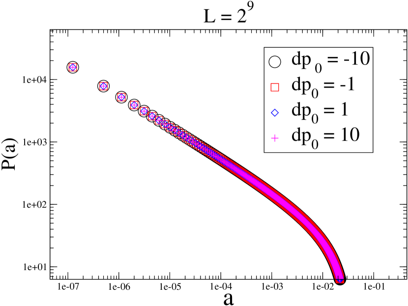
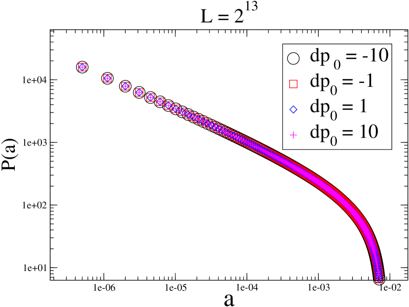
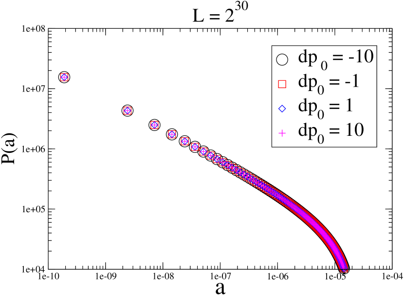
Figure 1: Degree distribution derived from the solution of the IVP (27) for different values of $L=2^{9}$ (left), $2^{13}$ (center), and $2^{30}$ (right). The degree distribution does not depend on $\differential p_{0}$ and have a very similar behaviour across $L$.

The degree distribution $P(a=\frac{k}{2L})$ obtained from this method is presented in Fig. 1, where we see that, under normalization, the value of $\differential p_{0}$ does not influence the probability values. Furthermore, upon the rescalling $\bar{a}=a/a_{max}$ and $\bar{P}=P\sqrt{a_{max}}$, or similarly $\bar{y}=y/y_{max}$, the number of links $L$ does not alter the behaviour of the degree distribution, as seen in Fig. 3.

Another initial value condition we investigated was to consider every node in the graph to have at least one link,

$$\mathsf{p}(y=0)=0\mbox{\quad and\quad}\evaluated{\derivative{\mathsf{p}}{y}}_{y=0}=\differential p_{0}\ ,$$ (28)

The integration runs until $y=\sqrt{8}$, where $a=1$, and then normalized. Similarly to the previous case, the value of $\differential p_{0}$ does not interfere with the degree distribution after normalization, as shown in Fig. 3.

Distribution	$P(a)\propto$	Range	RMSE
Weibull($\bar{a}$; $\lambda$, $k$)	$\quantity(\frac{\bar{a}}{k})^{\lambda-1}e^{-\quantity(\frac{\bar{a}}{k})^{\lambda}}$	$\bar{a}\in(0,2\cdot 10^{-1}]$ in Fig. 3	0.045
Gamma($\bar{a}$; $\lambda$, $k$)	$\bar{a}^{-\lambda}e^{-k\bar{a}}$	$\bar{a}\in(0,8\cdot 10^{-1}]$ in Fig. 3	0.166
PLIEC($\bar{a}$; $\lambda$, $k$)	$\bar{a}^{-\lambda}e^{-k/\bar{a}}$	$\bar{a}\in[6\cdot 10^{-2},\ 2\cdot 10^{-2}]$ in Fig. 3	0.155
Power-Law($\bar{a}$; $\lambda$)	$\bar{a}^{-\lambda}$	$\bar{a}\in(0,5\cdot 10^{-3}]$ in Fig. 3	0.385
Weibull($a$; $\lambda$, $k$)	$\quantity(\frac{a}{k})^{\lambda-1}e^{-\quantity(\frac{a}{k})^{\lambda}}$	$a\in[10^{-4},10^{0}]$ in Fig. 3	0.118

Table 1: Summary of the degree distributions fit to the results of the IVPs (27) and (28). The chosen range takes into account the value of the root mean square error (RMSE), which is minimized relative to the entire range of $a$ in the plot.

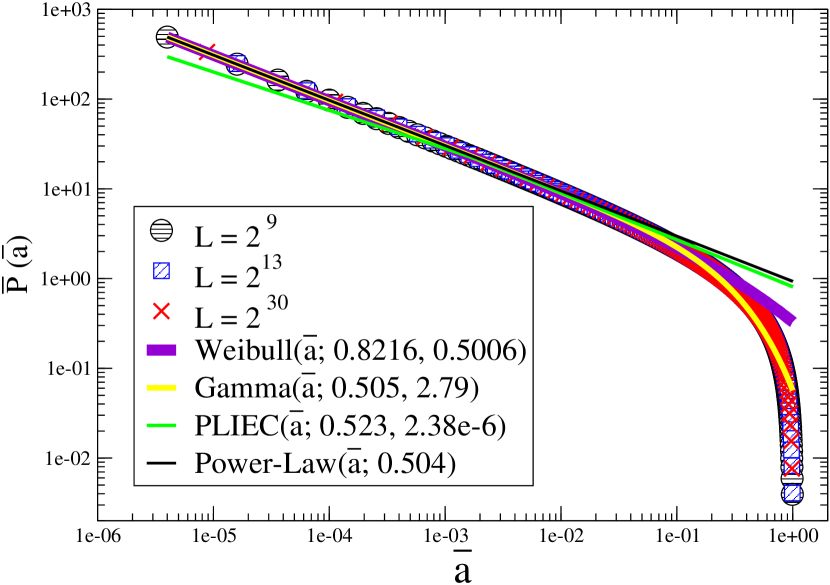
Figure 2: Re-scaled degree distribution for the IVP (27) irrespective of the number of links $L$. The result fits well with a Weibull and Gamma, also known as power law with cutoff, distributions within most of the allowed range.

Figure 3: Degree distribution derived from the solution of the IVP (28). The value of $\differential p_{0}$ does not interfere with the degree distribution. The result fits well with a Weibull distribution for a network with many links, $L>10^{4}$.

In Fig. 3 and Fig. 3 we fit our numerical results of $P(a)$ to some fat-tailed distributions. Namely we are interested in (i) a regular power law obtained as a result of preferential attachment [48]; (ii) the power law with exponential cutoff – Gamma distribution – and (iii) the Weibull distribution, both reported to be found in real-world networks [51]; (iv) the power law with inverse exponential cutoff (PLIEC) found to be the result of an entropic coarse-graining on networks ensembles obtained from constraints on the node degrees [31]. In Table 1 we present the range – region at which the distribution is valid, chosen based on the values of $a$ that minimize the root mean squared error (RMSE) between the functional form and the numerical results – for which each distribution compares to our numerical result for $P(a)$. The fact that for Fig. 3 the solutions start from above zero means that the degree distribution is considered from the minimal possible non-zero connectivity, $k=1$. Also, the case where every node has at least one link only fits with a real-world degree distribution for networks with $L>10^{4}$ links. Note from (26) that the metric leads to a natural power law behavior as $a^{-0.5}$, which was found throughout most of Fig. 3 range.

5 Conclusions

We presented an entropic dynamics of graphs with a fixed number of nodes $N$ and links $L$. This model leads to the Gibbs distribution (8) whose information metric is given by (13). When the dynamical assumption is that we evolve the parameters continuously and constrained in the statistical manifold we are lead into the Fokker-Planck equation (22). Steady-state solutions for two different IVPs are presented: The differential equation results for (27) are graphically represented in Fig. 1 and fitted for Weibull and Gamma distributions in Fig. 3. Also, the results differential equation for (28) fitted for the Weibull distribution are presented in Fig.3, where the real-world distribution is only valid for graphs with many $L>10^{4}$ links.

Our result is an information theory approach for dynamics of networks in which, under very general assumptions, the power law behavior emerges. Naturally, this work is not the single dynamical process possible. Under entropic dynamics, other random graph models can be studied and other constraints – instead of or in addition to (18) – can be implemented when maximizing the dynamical entropy $\mathsf{S}$ as in (16). This brings a perspective that the present article can be seen as an example on the ability to obtain dynamical process in complex systems using information theory. Therefore, building on the work presented here, we believe entropic dynamics gives a framework able to address the overarching need for dynamical models of networks.

References

- [1] Jaynes, E. T. Information theory and statistical mechanics. I. Physical Review 106, 620, DOI: 10.1103/PhysRev.106.620 (1957).
- [2] Jaynes, E. T. Information theory and statistical mechanics. II. Physical Review 108, 171, DOI: 10.1103/PhysRev.108.171 (1957).
- [3] Andersen, E. B. Sufficiency and exponential families for discrete sample spaces. Journal of the American Statistical Association 65, 1248–1255, DOI: 10.1080/01621459.1970.10481160 (1970).
- [4] Shore, J. & Johnson, R. Axiomatic derivation of the principle of maximum entropy and the principle of minimum cross-entropy. IEEE Transactions on information theory 26, 26–37, DOI: 10.1109/TIT.1980.1056144 (1980).
- [5] Skilling, J. The Axioms of Maximum Entropy. In Erickson, G. J. & Smith, C. R. (eds.) Maximum-Entropy and Bayesian Methods in Science and Engineering, vol. 31-32, 173–187, DOI: 10.1007/978-94-009-3049-0˙8 (Springer, Dordrecht, 1988).
- [6] Caticha, A. Relative Entropy and Inductive Inference. In AIP Conference Proceedings, vol. 707, 75–96, DOI: 10.1063/1.1751358 (American Institute of Physics, 2004).
- [7] Vanslette, K. Entropic updating of probabilities and density matrices. Entropy 19, 664, DOI: 10.3390/e19120664 (2017).
- [8] Golan, A. Information and Entropy Econometrics — A Review and Synthesis. Foundations and Trends(R) in Econometrics 2, 1–145, DOI: 10.1561/0800000004 (2008).
- [9] Caticha, A. & Golan, A. An entropic framework for modeling economies. Physica A: Statistical Mechanics and its Applications 408, 149–163, DOI: 10.1016/j.physa.2014.04.016 (2014).
- [10] Harte, J. Maximum entropy and ecology: a theory of abundance, distribution, and energetics (OUP Oxford, 2011).
- [11] Bertram, J., Newman, E. A. & Dewar, R. C. Comparison of two maximum entropy models highlights the metabolic structure of metacommunities as a key determinant of local community assembly. Ecological Modelling 407, 108720, DOI: 10.1016/j.ecolmodel.2019.108720 (2019).
- [12] De Martino, A. & De Martino, D. An introduction to the maximum entropy approach and its application to inference problems in biology. Heliyon 4, e00596, DOI: 10.1016/j.heliyon.2018.e00596 (2018).
- [13] Dixit, P. D., Lyashenko, E., Niepel, M. & Vitkup, D. Maximum entropy framework for predictive inference of cell population heterogeneity and responses in signaling networks. Cell Systems 10, 204–212, DOI: 10.1101/137513 (2020).
- [14] Vicente, R., Susemihl, A., Jericó, J. P. & Caticha, N. Moral foundations in an interacting neural networks society: A statistical mechanics analysis. Physica A: Statistical Mechanics and its Applications 400, 124–138, DOI: 10.1016/j.physa.2014.01.013 (2014).
- [15] Alves, F. & Caticha, N. Sympatric multiculturalism in opinion models. In AIP Conference Proceedings, vol. 1757, 060005, DOI: 10.1063/1.4959064 (AIP Publishing LLC, 2016).
- [16] Wilson, A. A statistical theory of spatial distribution models. Transportation Research 1, 253–269, DOI: 10.1016/0041-1647(67)90035-4 (1967).
- [17] Yong, N., Ni, S., Shen, S. & Ji, X. An understanding of human dynamics in urban subway traffic from the maximum entropy principle. Physica A: Statistical Mechanics and its Applications 456, 222–227, DOI: 10.1016/j.physa.2016.03.071 (2016).
- [18] Caticha, A. & Giffin, A. Updating Probabilities. In AIP Conference Proceedings, vol. 872, 31–42, DOI: 10.1063/1.2423258 (American Institute of Physics, 2006).
- [19] Barber, D. Bayesian Reasoning and Machine Learning (Cambridge University Press, 2012).
- [20] Skilling, J. & Bryan, R. K. Maximum entropy image reconstruction: general algorithm. Monthly Notices of the Royal Astronomical Society 211, 111–124, DOI: 10.1093/mnras/211.1.111 (1984).
- [21] Higson, E., Handley, W., Hobson, M. & Lasenby, A. Bayesian sparse reconstruction: a brute-force approach to astronomical imaging and machine learning. Monthly Notices of the Royal Astronomical Society DOI: 10.1093/mnras/sty3307 (2018).
- [22] Goodfellow, I., Bengio, Y. & Courville, A. Deep Learning (MIT Press, 2016). http://www.deeplearningbook.org.
- [23] Bahri, Y. et al. Statistical mechanics of deep learning. Annual Review of Condensed Matter Physics 11, 501–528, DOI: 10.1146/annurev-conmatphys-031119-050745 (2020).
- [24] Park, J. & Newman, M. E. J. Statistical mechanics of networks. Physical Review E 70, DOI: 10.1103/physreve.70.066117 (2004).
- [25] Bianconi, G. The entropy of randomized network ensembles. EPL (Europhysics Letters) 81, 28005, DOI: 10.1209/0295-5075/81/28005 (2007).
- [26] Bianconi, G. Entropy of network ensembles. Physical Review E 79, DOI: 10.1103/physreve.79.036114 (2009).
- [27] Anand, K. & Bianconi, G. Entropy measures for networks: Toward an information theory of complex topologies. Physical Review E 80, DOI: 10.1103/physreve.80.045102 (2009).
- [28] Anand, K., Bianconi, G. & Severini, S. Shannon and von Neumann entropy of random networks with heterogeneous expected degree. Physical Review E 83, DOI: 10.1103/physreve.83.036109 (2011).
- [29] Peixoto, T. P. Entropy of stochastic blockmodel ensembles. Physical Review E 85, DOI: 10.1103/physreve.85.056122 (2012).
- [30] Cimini, G. et al. The statistical physics of real-world networks. Nature Reviews Physics 1, 58–71, DOI: 10.1038/s42254-018-0002-6 (2019).
- [31] Radicchi, F., Krioukov, D., Hartle, H. & Bianconi, G. Classical information theory of networks. Journal of Physics: Complexity 1, 025001, DOI: 10.1088/2632-072x/ab9447 (2020).
- [32] Jaynes, E. T. Gibbs vs boltzmann entropies. American Journal of Physics 33, 391–398, DOI: 10.1119/1.1971557 (1965).
- [33] Caticha, A. Entropic dynamics, time and quantum theory. Journal of Physics A: Mathematical and Theoretical 44, 225303, DOI: 10.1088/1751-8113/44/22/225303 (2011).
- [34] Caticha, A. The entropic dynamics approach to quantum mechanics. Entropy 21, 943, DOI: 10.3390/e21100943 (2019).
- [35] Ipek, S., Abedi, M. & Caticha, A. Entropic dynamics: reconstructing quantum field theory in curved space-time. Classical and Quantum Gravity 36, 205013, DOI: 10.1088/1361-6382/ab436c (2019).
- [36] Pessoa, P. & Caticha, A. Exact renormalization groups as a form of entropic dynamics. Entropy 20, 25, DOI: 10.3390/e20010025 (2018).
- [37] Abedi, M. & Bartolomeo, D. Entropic dynamics of exchange rates and options. Entropy 21, 586, DOI: 10.3390/e21060586 (2019).
- [38] Caticha, N. Entropic dynamics in neural networks, the renormalization group and the hamilton-jacobi-bellman equation. Entropy 22, 587, DOI: 10.3390/e22050587 (2020).
- [39] Pessoa, P., Costa, F. X. & Caticha, A. Entropic dynamics on Gibbs statistical manifolds (2020). Under Review, preprint available: arXiv, 2008.04683.
- [40] Caticha, A. The basics of information geometry. In AIP Conference Proceedings, vol. 1641, 15–26, DOI: 10.1063/1.4905960 (American Institute of Physics, 2015).
- [41] Amari, S. Information geometry and its applications (Springer, 2016).
- [42] Ay, N., Jost, J., Lê, H. V. & Schwachhöfer, L. Information Geometry (Springer International Publishing, 2017).
- [43] Nielsen, F. An elementary introduction to information geometry. Entropy 22, 1100, DOI: 10.3390/e22101100 (2020).
- [44] Ay, N., Olbrich, E., Bertschinger, N. & Jost, J. A geometric approach to complexity. Chaos: An Interdisciplinary Journal of Nonlinear Science 21, 037103, DOI: 10.1063/1.3638446 (2011).
- [45] Felice, D., Mancini, S. & Pettini, M. Quantifying networks complexity from information geometry viewpoint. Journal of Mathematical Physics 55, 043505, DOI: 10.1063/1.4870616 (2014).
- [46] Franzosi, R., Felice, D., Mancini, S. & Pettini, M. Riemannian-geometric entropy for measuring network complexity. Physical Review E 93, DOI: 10.1103/physreve.93.062317 (2016).
- [47] Felice, D., Cafaro, C. & Mancini, S. Information geometric methods for complexity. Chaos: An Interdisciplinary Journal of Nonlinear Science 28, 032101, DOI: 10.1063/1.5018926 (2018).
- [48] Barabási, A.-L. & Albert, R. Emergence of scaling in random networks. Science 286, 509–512, DOI: 10.1126/science.286.5439.509 (1999).
- [49] Bianconi, G. & Barabási, A.-L. Bose-einstein condensation in complex networks. Physical Review Letters 86, 5632–5635, DOI: 10.1103/physrevlett.86.5632 (2001).
- [50] Albert, R. & Barabási, A.-L. Statistical mechanics of complex networks. Reviews of Modern Physics 74, 47–97, DOI: 10.1103/revmodphys.74.47 (2002).
- [51] Broido, A. D. & Clauset, A. Scale-free networks are rare. Nature Communications 10, DOI: 10.1038/s41467-019-08746-5 (2019).
- [52] Clauset, A., Shalizi, C. R. & Newman, M. E. J. Power-law distributions in empirical data. SIAM Review 51, 661–703, DOI: 10.1137/070710111 (2009).
- [53] Barabási, A.-L. Love is All You Need https://www.barabasilab.com/post/love-is-all-you-need (2018).
- [54] Holme, P. Rare and everywhere: Perspectives on scale-free networks. Nature Communications 10, DOI: 10.1038/s41467-019-09038-8 (2019).
- [55] Molontay, R. & Nagy, M. Two decades of network science: As seen through the co-authorship network of network scientists. In Proceedings of the 2019 IEEE/ACM International Conference on Advances in Social Networks Analysis and Mining, ASONAM ’19, 578–583, DOI: 10.1145/3341161.3343685 (2019).
- [56] Goh, K.-I. et al. The human disease network. Proceedings of the National Academy of Sciences 104, 8685–8690, DOI: 10.1073/pnas.0701361104 (2007).
- [57] Stella, M., de Nigris, S., Aloric, A. & Siew, C. S. Q. Forma mentis networks quantify crucial differences in STEM perception between students and experts. PLOS ONE 14, e0222870, DOI: 10.1371/journal.pone.0222870 (2019).
- [58] Pressé, S., Ghosh, K., Lee, J. & Dill, K. A. Nonadditive entropies yield probability distributions with biases not warranted by the data. Physical Review Letters 111, DOI: 10.1103/physrevlett.111.180604 (2013).
- [59] Pressé, S. Nonadditive entropy maximization is inconsistent with bayesian updating. Physical Review E 90, DOI: 10.1103/physreve.90.052149 (2014).
- [60] Oikonomou, T. & Bagci, G. B. Rényi entropy yields artificial biases not in the data and incorrect updating due to the finite-size data. Physical Review E 99, DOI: 10.1103/physreve.99.032134 (2019).
- [61] Pessoa, P. & Costa, B. A. Comment on “black hole entropy: A closer look”. Entropy 22, 1110, DOI: 10.3390/e22101110 (2020).
- [62] Fisher, R. A. Theory of statistical estimation. Mathematical Proceedings of the Cambridge Philosophical Society 22, 700–725, DOI: 10.1017/S0305004100009580 (1925).
- [63] Rao, C. R. Information and the accuracy attainable in the estimation of statistical parameters. In Bulletin of Calcutta Mathematical Society, vol. 37, 81, DOI: 10.1007/978-1-4612-0919-5“˙16 (1945).
- [64] Cencov, N. N. Statistical decision rules and optimal inference. Transl. Math. Monographs, vol. 53, Amer. Math. Soc., Providence-RI (1981).
- [65] Campbell, L. L. An extended Čencov characterization of the information metric. Proceedings of the American Mathematical Society 98, 135–141, DOI: 10.2307/2045782 (1986).
- [66] Nelson, E. Quantum fluctuations (Princeton University Press, 1985).