MUFASA: Multimodal Fusion Architecture Search for Electronic Health Records

Abstract

One important challenge of applying deep learning to electronic health records (EHR) is the complexity of their multimodal structure. EHR usually contains a mixture of structured (codes) and unstructured (free-text) data with sparse and irregular longitudinal features – all of which doctors utilize when making decisions. In the deep learning regime, determining how different modality representations should be fused together is a difficult problem, which is often addressed by handcrafted modeling and intuition. In this work, we extend state-of-the-art neural architecture search (NAS) methods and propose MUltimodal Fusion Architecture SeArch (MUFASA) to simultaneously search across multimodal fusion strategies and modality-specific architectures for the first time. We demonstrate empirically that our MUFASA method outperforms established unimodal NAS on public EHR data with comparable computation costs. In addition, MUFASA produces architectures that outperform Transformer and Evolved Transformer. Compared with these baselines on CCS diagnosis code prediction, our discovered models improve top-5 recall from 0.88 to 0.91 and demonstrate the ability to generalize to other EHR tasks. Studying our top architecture in depth, we provide empirical evidence that MUFASA’s improvements are derived from its ability to both customize modeling for each data modality and find effective fusion strategies.

1 Introduction

In recent years, hospitals have begun adopting electronic health record (EHR) systems (Adler-Milstein et al. 2015). This digitization of large amounts of medical data offers an unprecedented opportunity for deep learning to improve healthcare, such as by predicting diagnoses (Lipton et al. 2015; Miotto et al. 2016), reducing healthcare costs (Bates et al. 2014; Krumholz 2014), and modeling the temporal correlation among medical events (Che et al. 2018; Xue et al. 2020). However, EHR data’s intrinsic longitudinal and multimodal nature adds distinct complexity that is absent from common academic datasets, such as ImageNet and WMT, that are often used to develop machine learning models.

Reflecting the complexity of real-world medical information, EHR data contains multiple modalities, both structured (codes and labs) and unstructured (free-text) (Figure 1). For instance, EHR usually contains: (1) contextual features, such as patient age and sex; (2) longitudinal categorical features, such as procedure codes, medication codes, and condition codes; (3) longitudinal continuous features, such as blood pressure, body temperature, and heart rate; and (4) longitudinal free-text clinical notes, which are often lengthy and contain a lot of medical terminology. These data types differ not only in feature spaces and dimensionalities, but also in data generation processes and measurement frequencies. For example, lab tests and procedures are ordered at the physician’s discretion, while blood pressure and body temperature can be monitored on an hourly basis.

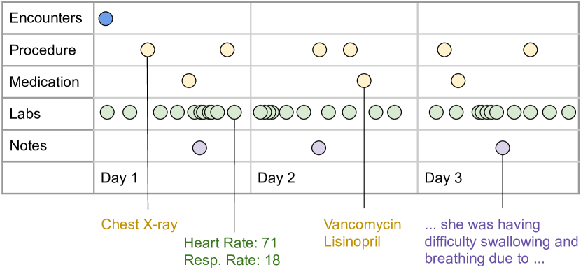
Figure 1: An illustrative example of a patient’s record. It contains multiple feature modalities, including categorical features, continuous features and clinical notes across time.

Synthesizing complimentary information across these multiple modalities allows doctors to make higher quality decisions. For instance, lab tests (continuous features) provide detailed information about a patient’s physiological condition, while diagnosis codes (categorical features) capture a system-level view of the patient’s state. These modalities have complex interactions; for example, a patient’s lab results and diagnoses should be considered when trying to predict what effect a blood pressure medication would have on them. Doctors consider this diverse data, as well as previous doctors’ notes, when making decisions. Thus, modeling these modalities jointly has strong machine learning potential, but needs to be done with care, as adding modalities naively risks making overall model performance worse (Ramachandram and Taylor 2017; Baltrušaitis, Ahuja, and Morency 2018). Three questions that guide multimodal modeling are: (1) What model architecture best suits a given modality? For example, convolutional architectures are commonly applied to images, while recurrent neural networks are typically used for temporal data. These decisions are usually based on researchers’ intuitions. (2) Which modalities should be fused together? “Fusion” refers to the joint modeling of multiple modalities at once by combining their feature embeddings; popular deep learning fusion operations include addition and concatenation. An example policy is given by Neverova et al. (2015), who argue that highly correlated modalities should be fused together. (3) When we do perform modality fusion, at what point in modeling should it occur? Available fusion strategies are data-level or early fusion (Valada et al. 2016; Rajkomar et al. 2018); intermediate-level or hybrid fusion (Liang et al. 2014; Liu et al. 2014); and classifier-level or late fusion (Kahou et al. 2016; Simonyan and Zisserman 2014) (See Figure 2 for an example of each strategy).

Thus far, these questions have been addressed by expert hand-designed architectures, which vary from task to task. In this work, we aim to create a generalizable framework to automatically perform this multimodal modeling without meticulous human design. To do this, we look towards neural architecture search (NAS) (Yao 1999), which has recently produced state-of-the-art results on academic datasets (Real et al. 2019). However, existing NAS works have primarily focused on unimodal data, and so our focus on applying these techniques to real-world EHR data requires us to offer solutions to tackle the complexities of multimodality.

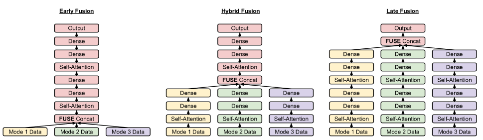
Figure 2: Example of different fusion strategies using a Transformer base architecture. In each depiction, yellow represents modeling only applied to Mode 1, green Mode 2, and purple Mode 3. Red represents modeling applied to all three modes jointly.

We propose MUltimodal Fusion Architecture SeArch (MUFASA), which expands the contemporary NAS paradigm to simultaneously optimize multimodal fusion strategies; that is, we jointly search for multiple independent modality-specific architectures, as well as the fusion strategy to combine those architectures at the right representation level. We base our searched models on the Transformer (Vaswani et al. 2017) because recent works have shown it can implicitly leverage EHR’s internal structure (Choi et al. 2018, 2019). Our experimental results show that our discovered MUFASA models outperform Transformer, Evolved Transformer, RNN variants, and models discovered using traditional NAS, on public EHR data. Specifically, compared with Transformer on Clinical Classifications Software (CCS) diagnosis code prediction, MUFASA architectures improve test set top-5 recall from 0.8756 to 0.9075. In addition, we empirically demonstrate that MUFASA outperforms unimodal NAS by customizing each modality specifically – an ability not available to traditional NAS. Comparing search performance with unimodal NAS on the CCS task, MUFASA improves validation top-5 recall from 0.9025 to 0.9134 with comparable search costs. What’s more, MUFASA architectures demonstrate more effective transfer to ICD-9, a different EHR task that we do not search on directly. Our contributions are summarized as follows:

• MUFASA, the first multimodal NAS that jointly optimizes fusion strategy and modality-specific architectures.

• A novel search space that jointly searches unique architectures for distinct modalities and the best strategies to fuse those architectures at the right representation level.

• Empirical evidence demonstrating that MUFASA is superior to traditional NAS for EHR data with comparable computation costs. This includes showing that MUFASA architectures indeed achieve improvements by customizing modeling for each modality.

2 Related Works

Recently, machine learning researchers have begun to leverage the multimodal nature of EHR to improve prediction performance (Shin et al. 2019). Xu et al. (2018) use both continuous patient monitoring data, such as electrocardiograms, and discrete clinical events to better forecast the length of ICU stays. Qiao et al. (2019) propose multimodal attentional neural networks to combine information from medical codes and clinical notes, which improves diagnosis prediction. As highlighted by these authors, there are few works integrating streaming and discrete EHR data (Xu et al. 2018), or clinical text and discrete EHR data (Qiao et al. 2019). Our work focuses on integrating clinical notes, continuous data, and discrete data all together. Additionally, in contrast to these manually designed multimodal architectures, we explore NAS to automatically learn architectures that leverage the multimodal nature of EHR.

Our work also builds upon neural architecture search (NAS). Recent results shows that automatically designed deep learning models can achieve state-of-the-art performance on academic benchmarks (Zoph and Le 2016; Real et al. 2019), as well as offer practical usage (Tan and Le 2019). One-shot NAS methods (Bender et al. 2018) attempt to radically reduce the amount of compute needed to run searches by not training each candidate individually; here, we use a relatively low compute task and so do not need to employ these methods. Within this NAS field, our work is most closely related to two others. The first is So, Liang, and Le (2019), who apply NAS to search for a Transformer architecture on NLP data. Our work differs in that we expand our search to include multimodal fusion strategies and modality-specific architectures; in Section 5 we compare our search methodology to their unimodal setup and our resulting architectures to the product of their search, the Evolved Transformer. The second comparable work is Pérez-Rúa et al. (2019), who use architecture search to optimize multimodal feature fusion in image classification models. However, they use off-the-shelf pretrained models as building blocks and only search over their fusion points. In contrast, we are the first work to jointly optimize multimodal fusion strategies and modality-specific architectures together; this allows us to not only optimize how modalities are fused, but also the type of deep learning computation applied to each modality. Additionally, our focus is on sequence models for EHR data, not convolution-based models for images.

3 Methods

In this section, we briefly describe evolutionary NAS (Real et al. 2019) and the building blocks of our search space. We also describe MUFASA, our main methodological contribution.

3.1 Evolutionary Neural Architecture Search

We use the tournament selection evolutionary architecture search algorithm proposed by Real et al. (2019). In this framework, candidate architectures are represented as the gene encodings of individuals; see Section 3.3 for a description of these encodings. An initial population is created of random or pseudo-random individuals; in our case we use the warm-start NAS method (So, Liang, and Le 2019) by seeding the initial population with a known strong architecture, the Transformer. From there, evolution begins by assigning every individual in the population a fitness. These fitnesses are determined by building the architectures described by each individual’s gene encoding and training the resulting models on training data. The models are then evaluated on validation data to determine the individuals’ fitnesses. Once fitnesses are assigned, a tournament is conducted by sampling $T$ random individuals from the population and selecting the one with the highest fitness to be a parent. This parent is mutated, with its gene encoding fields randomly changed according to a mutation rate, to produce a child. The child is assigned a fitness in the same fashion as the parent. Then another tournament is conducted by sampling $T$ random individuals from the population and having the one with the lowest fitness killed, meaning removed from the population. The newly created and evaluated child is then added to the population in the killed individual’s place. This cycle of child creation and weak individual removal is repeated, creating a population of high fitness individuals, which for NAS means strongly performing architectures (Algorithm 1 in Appendix).

3.2 MUFASA

To adapt to multimodal data, we reformulate the NAS search space to also include fusion strategy search. To do this, instead of searching for a single architecture, we search for several architectures simultaneously: one for each individual data modality and a special fusion architecture that is responsible for fusing data modalities together and performing further processing. Put formally, the standard NAS objective is to find an optimal neural network function (architecture) $f_{A}(x;\theta)$, parameterized by weights $\theta$, that transforms the input $x$ to a representation that is more amenable for a target task. A majority of NAS work, which has focused on unimodal datasets, searches for a single monolithic $f^{\prime}$. Likewise, several EHR works treat modalities identically, combining all $M$ data modalities together via a simplistic combiner function, such as vector concatenation (Lipton et al. 2015; Rajkomar et al. 2018; Choi et al. 2016; Li et al. 2019), before passing them to one cohesive model (early fusion):

$$f_{A}(x;\theta)=f^{\prime}(\operatorname{concat}(x_{0},x_{1},\dots x_{M-1});\theta)$$

Here, we decompose our target architecture into a series of modality architectures, $g_{i}$, that are applied independently to each corresponding $i$th data modality. We additionally define $h$ as the special fusion architecture that takes the outputs of each $g_{i}$ and jointly transforms them into the final output:

$$f_{A}(x;\theta)=h(g_{0}(x_{0};\theta_{0}),\dots g_{M-1}(x_{M-1};\theta_{M-1});\theta_{h})$$

During search, MUFASA searches for the fusion architecture, $h$, and every modality architecture, $g_{i}$ (Figure 3). This reformulates the search space, distinguishing MUFASA from previous NAS works. The basis for this reformulation is the notion that for complex data such as EHR, deep learning transformations should be specific to their input modalities; this is represented by the independent modality architectures. As previously mentioned, EHR categorical features, continuous features and clinical notes have different data representations and generative processes; that they would each benefit from distinct types of modeling is intuitive. Joint modeling across modalities is also beneficial, but needs to be applied at the right depth; the fusion architecture embodies this mentality.

In Section 5, we share empirical evidence that supports these ideas that (i) distinct modeling for each modality is beneficial, (ii) proper fusion strategy is critical to model performance, and (iii) the MUFASA search space is superior to the unimodal NAS space for EHR data, when controlling for search costs.

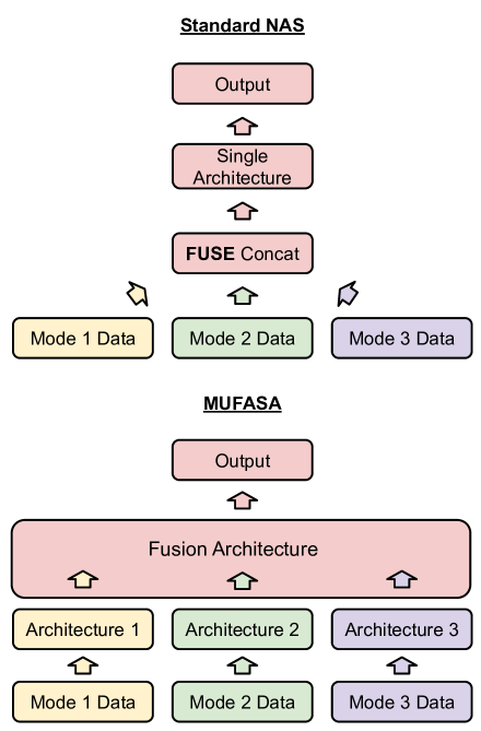
Figure 3: Standard NAS searches for a single unimodal architecture. MUFASA searches for independent architectures for each data modality, as well as a Fusion Architecture to tie those modal architectures together.

The utility of MUFASA’s multi-architecture search is its ability to jointly represent and search over several fusion strategies while performing regular architecture search. In the next subsection, we describe how we construct architectures using typical NAS blocks. Note here that every architecture can be reduced to an identity transformation or, in the case of the fusion architecture, a simple concatenation to perform early fusion. There is a shared parameter budget for the entire model, but there is no explicit constraint on how those parameters can be allocated.

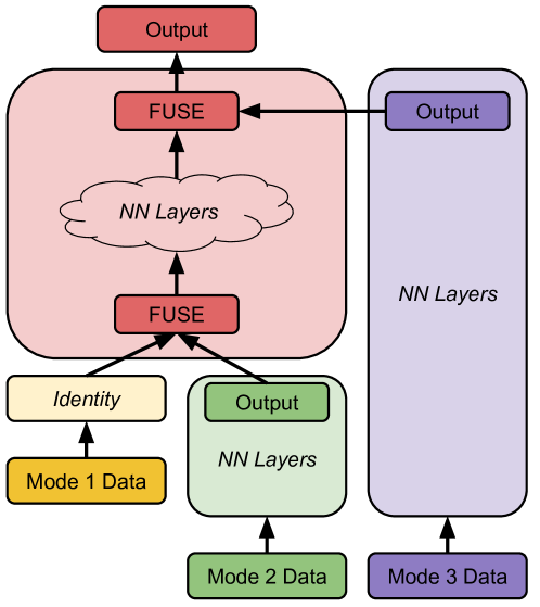
Figure 4: MUFASA example architecture that employs all three fusion types. Mode 1 utilizes early fusion, as its modality architecture is an identity transformation and thus it is fused with Mode 2 before it passes through any neural network (NN) layers. Mode 2 utilizes hybrid fusion, as it first passes through its own non-identity modality architecture before being fused with Mode 1 and transformed by the fusion architecture (in red). Mode 3 utilizes late fusion, as it only receives processing through its independent modality architecture, before being fused with the final output.

3.3 Architecture Blocks

Similar to previous works, each of the architectures in our search space is composed of blocks (Figure 5). Each block receives two hidden state inputs and generates a new hidden state output. The block is a computation unit that transforms each input separately and then combines two transformed outputs together to generate the final block output. The computation applied to each input is called a branch. The outputs of both branches are combined via the ‘combiner function’. The search space for a single block contains $1$ block-level search field (combiner function) and $5$ branch-level search fields (input, normalization, layers, output dimension, and activation) for each of the two branches (10 branch-level fields total). ‘Input’ specifies which previously generated hidden state will be fed into the branch.

Different from previous architecture search work, MUFASA defines two types of blocks, as depicted in Figure 5. For modality-specific architecture blocks, only hidden states from the same modality can be inputs. For fusion architecture blocks, both fusion architecture hidden states and modality architecture states can be inputs. Fusion architecture blocks are constructed after the modality-specific blocks have been constructed. These input constraints ensure 1) an independent set of blocks for each modality and 2) that the fusion architecture can access the modality architectures at any representation level, as described by the multi-architecture search space in Section 3.2. Any orphaned hidden outputs are then fused with the model output. A gene encoding for a single block is represented as {left input, left normalization, left layer, left relative output dimension, left activation, right input, right normalization, right layer, right relative output dimension, right activation, combiner function}. In total, MUFASA has a search space of $1.76\times 10^{23}$ models (See Appendix for more vocabulary and search space information).

The fusion architecture can incorporate the modality architectures’ outputs at any point in its own architecture; for instance, the fusion architecture can pass the Mode 1 output through its very first neural network layer, and still delay inclusion of the Mode 3 output until the final model layer. It is through being able to freely adjust these two aspects of architecture - parameter allocation and modality inclusion points - that all multimodal fusion strategies can be expressed and searched for via evolution. See Figure 4 for an example of how early, hybrid, and late fusion are all achieved. Note, not only can all fusion strategies be represented, but different fusion strategies can be assigned to different modalities. In Section 5 we detail the particularly interesting case in which the strongest model we found using MUFASA applies two different fusion strategies to the same modality (Figure 6).

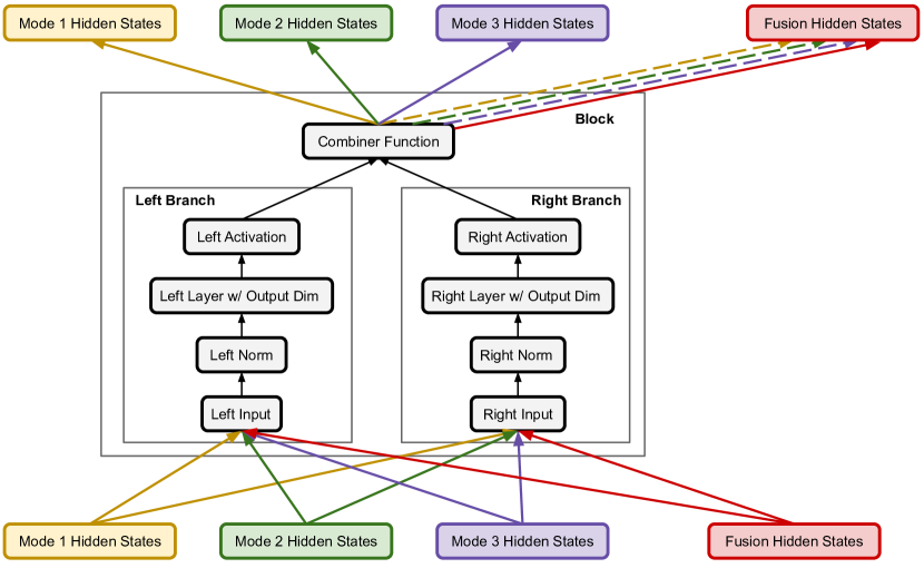
Figure 5: Search block structure. In MUFASA, each modality can access only the previous hidden states from that same modality. The fusion architecture can access fusion architecture states, as well as states from the modality architectures.

4 Experiment Setup

4.1 Dataset and Prediction Tasks

Dataset

We use the Medical Information Mart for Intensive Care (MIMIC-III) (Johnson et al. 2016) dataset. It contains single-center real-world EHR data for 53,423 hospital admissions, admitted to critical care units from 2001 to 2012 (See Table 8 in Appendix). We represent patient’s medical histories in Fast Healthcare Interoperability Resources (FHIR) format (Mandel et al. 2016), as described by Rajkomar et al. (2018). After data pre-processing, we have 40,511 patients and 51,081 admissions. For all tasks, data is randomly split into train, validation and test sets in an $8:1:1$ ratio.

Feature Modalities

We use three feature modalities for the sequence data: (1) Categorical sequence features, including diagnosis and procedure codes; medication request and administration codes; and admission sources. (2) Continuous sequence features, including lab test results and vital signs such as heart rate, respiratory rate, blood pressure, body temperature, and sodium levels, when they are available. (3) Free-text clinical notes. Before feeding this data to our models, we embed the categorical sequence features and clinical notes (trained from scratch). We normalize continuous feature values to Z-scores using training set statistics and clamp outliers 10 standard deviations away from the mean. For values that are missing at particular time steps, we use the last observed value for that signal. The outputs of the searched architectures constitute the sequence representations. After concatenating these representations with additional context features (such as age), we feed the output into dense layers to generate the final task predictions. More details can be found in Appendix Section 8.5.

Prediction Tasks

Our experiments focus on two diagnosis code prediction tasks at discharge time for each encounter:

• CCS:   Predicting the primary Clinical Classifications Software (CCS) diagnosis code (Elixhauser 1998). This is a multiclass problem and each hospital encounter has only one primary CCS code. Because there are over 250 possible diagnosis codes, we use top-5 recall (recall@5) as the main evaluation metric.

• ICD-9:   Predicting the International Classification of Diseases, 9th Revision (ICD-9) diagnosis code (Slee 1978). This is a multilabel problem, as one hospital encounter could have several of the 14,000 available ICD-9 diagnosis codes. We use AUCPR as the main evaluation metric.

4.2 Baseline Search Algorithms and Model Architectures

The baseline models that we compare against are the original Transformer (Vaswani et al. 2017), LSTMs (Rajkomar et al. 2018), attentional bidirectional LSTMs (Qiao et al. 2019) and the Transformer NAS variant, the Evolved Transformer, which was searched for on translation data. To demonstrate the effectiveness of our MUFASA search method, we compare it against the same unimodal NAS setup that was used by So, Liang, and Le (2019), but using our search space vocabulary (Appx. Table 5). This baseline NAS method is not amenable to multimodal inputs and so we concatenate the inputs together before feeding them into each candidate model, as is standard practice in EHR literature (Lipton et al. 2015; Rajkomar et al. 2018; Choi et al. 2016; Li et al. 2019).

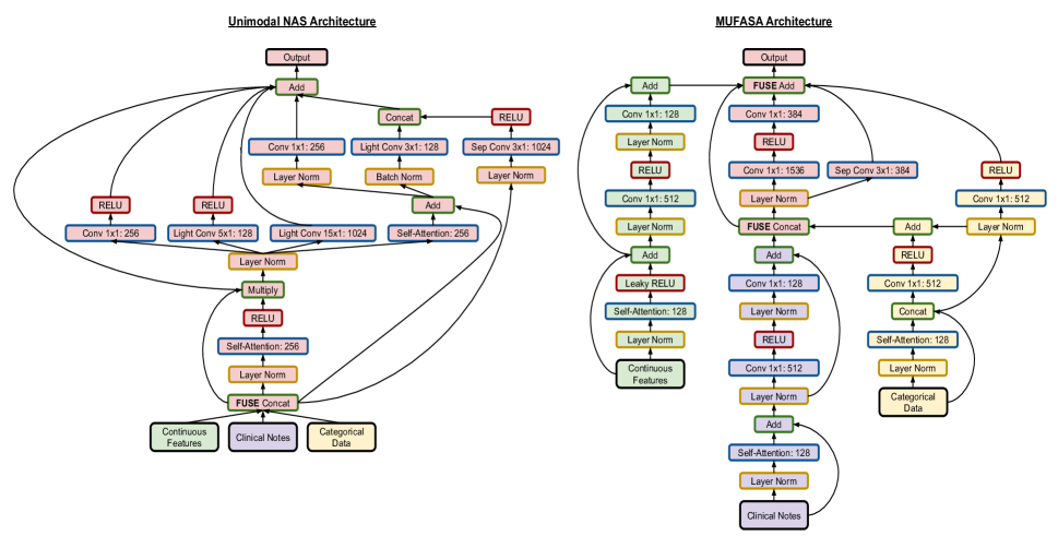
Figure 6: Discovered model architectures from unimodal NAS and MUFASA on the MIMIC CCS task. The border color of each node represents the type of function applied: yellow for normalization, red for nonlinearity, blue for neural network layer, and green for branch combiner. The color shading for each node represents the data that flows through that node: green is continuous features, purple is clinical notes, yellow is categorical data, and red is multimodal. For MUFASA, the color shading also indicates which architecture the node is a part of; green, purple and yellow denote the independent modal architectures and red is the fusion architecture. The MUFASA architecture is much more flexible in terms of what it can represent and applies unique neural architectures to each data modality. In addition, MUFASA applies different fusion strategies to each modality. For example, the continuous features are processed independently and are only joined with the other modalities at the very end via late fusion. The clinical notes, on the other hand, are processed independently at first, but then are joined with categorical data and processed jointly via hybrid fusion. The most interesting case is the categorical data architecture, which utilizes both hybrid and late fusion.

4.3 Architecture Search Configuration

We conduct architecture searches on MIMIC CCS. The search configurations are almost identical for MUFASA and our unimodal search baseline. Both employ the same search space and tournament selection NAS algorithm as described in Section 3. Each search uses 200 CPU workers for evaluating candidate models asynchronously. The population size is 100 and the tournament size is 30. We independently mutate each encoding field with a probability of $1.875\%$ and uniform randomly select its replacement from the possible vocabulary. For each individual architecture search, we train 5000 child models, which in every case appeared to reach convergence. In both searches the parameters for candidate models were not allowed to exceed 76 million. The total search times for both unimodal NAS and MUFASA are approximately the same: roughly 3 days. Unimodal NAS uses the early fusion Transformer to warm-start the search. To control for maximum model depth, MUFASA uses the Transformer hybrid fusion seed (Figure 2). See the Appendix for more details.

5 Results

5.1 MUFASA vs. Unimodal NAS

We first compare MUFASA to the equivalent unimodal NAS setup on MIMIC CCS. All relevant configurations, such as compute and hyperparameters, are identical for both searches. We run each search three times and calculate the fitness mean and standard deviation of the best models for each search method. Compared with unimodal search, MUFASA improves CCS validation top-5 recall from $0.9025~{}(0.0041)$ to $0.9134~{}(0.0034)$; this improvement is statistically significant under independent two-sample t-test with p-value threshold $0.05$. Figures 6 depicts the best architectures from each of the searches. Both architectures are substantially different from the original Transformer seeds, but in very different ways. The unimodal NAS output is “wider” than Transformer; it utilizes several wide convolutions and at many points processes the same hidden state through parallel neural network layers. Observing this pattern across multiple unimodal NAS searches, we interpret this as the architecture creating multiple “perspectives” for the same concatenated input, as it is unable to model the modalities individually. On the other hand, the MUFASA architecture scarcely performs parallel computation on the same state, but substantially silos the different modalities and assigns them each unique fusion strategies. For example, the continuous features are processed independently and are only joined with the other modalities at the very end via late fusion. Clinical notes, on the other hand, are processed independently at first, but then are joined with categorical data and processed jointly via hybrid fusion. The most interesting case is the categorical data architecture, which utilizes both hybrid and late fusion.

Table 1: Test set performance comparison among different model architectures (with different fusion strategies) for the CCS task. We use top-5 recall as the main evaluation metric. We report the mean and standard deviation from 3 runs for each model, with individually tuned hyperparameters. ^* denotes that the improvement is statistically significant under independent two-sample t-test with p-value threshold $0.05$.

Model	Parameters	Recall@5
LSTM	38.7M	0.8715 (0.0256)
Attentional bidirectional LSTM	42.7M	0.8506 (0.0028)
Transformer Small (Early)	12.7M	0.8338 (0.0020)
Transformer Default (Early)	24.5M	0.8340 (0.0051)
Transformer Small (Hybrid)	12.7M	0.8744 (0.0021)
Transformer Default (Hybrid)	24.7M	0.8756 (0.0039)
Transformer Small (Late)	11.7M	0.8727 (0.0041)
Transformer Default (Late)	24.8M	0.8740 (0.0025)
Evolved Transformer Small (Early)	11.5M	0.8372 (0.0032)
Evolved Transformer Default (Early)	25M	0.8315 (0.0030)
Evolved Transformer Small (Hybrid)	12.2M	0.8722 (0.0042)
Evolved Transformer Default (Hybrid)	24.6M	0.8711 (0.0035)
Unimodal NAS	12.4M	0.8841(0.0019)
MUFASA	11.5M	0.9075*(0.0021)

5.2 Architecture Study

Having demonstrated that MUFASA generates better search results than unimodal NAS, we now take a closer look at the architecture it produced and explore what makes that architecture effective. We begin with a comparison to other architectures that have been applied to EHR data, as well as other NAS baselines including the Evolved Transformer and our best unimodal NAS model (Table 1). Note that for the Transformer baselines, which we run at both the default Tensor2Tensor 2 layer size and a size comparable to those found by the searches, fusion strategy has a big impact on performance. Hybrid and late fusion are comparable, but significantly outperform early fusion; fusion strategy being key to model performance is one of the chief motivations for this work. In fact, fusion strategy is so crucial that in this particular case, early fusion performs worse than training on just categorical features or just clinical notes alone (Table 3); this may be due to the lack of neural network layers that are capable of doing efficient computation across disparate feature representations with different underlying distributions. The model learned by unimodal NAS outperforms all other baselines that use early fusion; this illustrates the power of EHR-specific modeling. By combining the benefits of both searching for a critically important fusion strategy and modality-specific modeling, MUFASA produces an architecture that substantially outperforms all other baselines.

Table 2: Testing Independent Modality Modeling: Input perturbation experiments using MUFASA architecture.

Perturbation	CCS Recall@5
MUFASA Baseline	0.9075 (0.0021)
Forced Early Fusion	0.8608 (0.0019)
Shuffle	0.8829 (0.0008)
Partial (Categorical $\rightarrow$ Notes)	0.9013 (0.0052)
Partial (Notes $\rightarrow$ Categorical)	0.8941 (0.0008)

Table 3: Single Modality Training: Transformer CCS training on each modality in isolation.

Modality	Recall@5
Categorical only	0.8665 (0.0030)
Continuous only	0.7003 (0.0056)
Notes only	0.8451 (0.0045)

The question still stands, however, as to how tailored the MUFASA architecture is to the individual EHR modalities; its performance on the target task is clearly strong, but how much of that comes from custom modeling for each data modality? To test this, we train three models with the same architecture but with alternative inputs, thereby highlighting the importance of each data modality being fed into its optimized path (Table 2). First, we perform a forced early fusion, whereby all input modalities are concatenated and fed into all input paths; this eliminates the isolated modeling of each modality. This experiment shows that the MUFASA architecture’s separate input processing is customized for each individual modality; passing all modalities into every input path together hurts performance. Second, we randomly shuffle the input modalities, passing each modality to a different modality’s input path; specifically, categorical features are fed into the continuous features path, continuous features are fed into the clinical notes path, and clinical notes are fed into the categorical features path. This maintains individual modeling for each modality, but changes that modeling from what MUFASA designates, providing evidence that customized modeling matters. Lastly, we strike a midway point between the first two experiments by performing a partial early fusion, adding just one modality to another modality’s input path; we randomly try (I) adding categorical features to the clinical notes input path and, in a separate training, (II) adding clinical notes to the categorical features path (for experimental symmetry). Table 2 shows these improper input routings can cause a statistically significant drop in quality. The only exception is Partial (Categorical$\rightarrow$Notes); however, this is likely because categorical features are stronger features than clinical notes (Table 3), so having clinical notes “share” parameters with categorical features is not as harmful. Note, this still supports the idea that modality-specific processing is sensitive, as the mirrored “sharing,” Partial (Notes$\rightarrow$Categorical), is significantly worse. Jointly, these results confirm our hypothesis that MUFASA’s improvements come not only from its independently modeling modalities, but also its customized modeling specifically for those modalities.

To understand if the discovered MUFASA modeling is effective beyond our target task, we test the generalizability of our discovered architectures on the yet unseen ICD-9 task. As shown in Table 4, MUFASA demonstrates a statistically significant improvement over the strongest baseline model. The unimodal NAS architecture also seems to generalize, outperforming the strongest early fusion baseline, but is unable to improve over the hybrid fusion Transformer, highlighting its limitations when fusion strategy plays an important role.

Table 4: Generalizability to ICD9 Task: Comparison between baselines and the CCS-searched models transferred to ICD-9. We train all the same models as in Table 1, using the same methodology, but only present the strongest baselines. ^* denotes the improvement is statistically significant under independent two-sample t-test with p-value threshold $0.05$.

Model	Parameters	AUCPR
Transformer Small (Early)	89.2M	0.3047 (0.0009)
Transformer Default (Hybrid)	101.3M	0.3273 (0.0012)
Unimodal NAS	89M	0.3200 (0.0016)
MUFASA	86M	0.3327* (0.0009)

6 Conclusion

Effective modelling of EHR data has great potential to advance healthcare, from improving diagnoses to suggesting treatments. However, its complex multimodal nature has required human experts to hand-design unorthodox models or use one-size-fits-all models – an approach that does not scale as medical data becomes richer. To address this, we proposed MUFASA to automatically design deep learning architectures that directly account for the uniqueness of different modalities. Our empirical results have shown (1) MUFASA is superior to unimodal NAS on MIMIC-III CCS; (2) the discovered MUFASA architectures can outperform commonly used baseline architectures and transfer improvements to other EHR tasks; and (3) the effectiveness of MUFASA is derived from its ability to specifically model various modalities and find effective fusion strategies. Future work can investigate applying MUFASA to other types of medical data modalities, including medical images, waveforms, and genomics.

7 Ethics

We see this work as being a positive step towards the democratization of AI, as it will allow non-experts to develop machine learning models for complex multimodal datasets. Although previous evolutionary NAS works have required hundreds of GPUs/TPUs to reach state-of-the-art performance on the most intensely studied academic datasets, we demonstrate that much less compute can be used ($\sim$ 2 CPU years) to improve performance in applied settings, on very important real-world datasets that do not receive as much attention. Lastly, we hope our contribution of applying machine learning to medical datasets helps advance healthcare for all patients. We only use fully de-identified data from MIMIC-III and follow the data agreement.

8 Appendix

8.1 More Search Space Information

As described in Section 3.3, our search space is composed of blocks. The encoding for a single block contains $1$ block-level search field (combiner function) and $5$ branch-level search fields (input, normalization, layers, output dimension, and activation) for each of the two branches (10 branch-level fields total). ‘Combiner function’ is the function applied to combine the outputs of both branches. ‘Input’ specifies which previously generated hidden state will be fed into the branch. ‘Normalization’ is the normalization immediately applied to the input, before any other transformation. ‘Layer’ is the neural network layer applied after normalization. ‘Output dimension’ defines the relative output dimension of the layer transformation (So, Liang, and Le 2019). ‘Activation’ is the non-linearity applied to the output of each layer. Together these components define the entire searchable architecture space. The vocabulary for our gene encodings is shown in Table 5.

Because MUFASA searches for multiple architectures simultaneously, we maintain separate sets of blocks for each individual architecture. Specifically, for our EHR tasks there are 3 distinct modes (Subsection 4.1) and so we maintain 4 distinct block sets: one for each of the 3 independent modality architectures and one for the fusion architecture. Unlike previous works that leverage similar spaces (Zoph et al. 2018; Real et al. 2019), we do not have the concept of a larger ‘cell’ that is stacked; our dataset is relatively small and so we find having additional stacked cells does not help.

8.2 Relationship Between Figures 3-5

Figures 3-5 all describe the same MUFASA search space, but at varying levels of abstraction. Figure 3 is the highest in abstraction, giving an overview of how the different types of MUFASA architectures (modality and fusion) interact; the modality architectures are independent, and the fusion architecture combines them together. Figure 4 gives a more concrete example with some “layers” exposed, showing how different fusion strategies can be achieved at a macro level. Figure 5 is the most granular, “zooming in” to what a search space block looks like and what inputs different MUFASA blocks can take while preserving the independence assumptions of the modality blocks.

8.3 Training Details

All training parameters are optimized on top of the default Tensor2Tensor hyperparameters (Vaswani et al. 2018) for a Transformer trained with an Adam optimizer (Kingma and Ba 2015). We additionally tune the learning rate schedule and batch size for all model trainings outside of searches. The possible learning rate schedules are constant, linear decay, exponential decay, single cycle cosine decay, and inverse-square-root decay. The possible batch sizes range from 16 to 512. We use a Gaussian process bandit optimization algorithm (Desautels, Krause, and Burdick 2014) to tune hyperparameters to maximize the model performance using evaluation results on the validation set. For search, we use the best baseline Transformer hyperparameters for all models; that is a single-cycle cosine decay learning rate schedule without warm-up, batch size 32, and an initial learning rate of $4.23\times 10^{-4}$. All models are trained until convergence.

Table 5: Architecture Vocabulary

Search Field	Vocabulary
Layer	• Standard convolution $s\times 1$ for $s\in\{1,3\}$ • Depthwise separable convolution (Sifre and Mallat 2014) $s\times 1$ for $s\in\{3,5,7,9,11\}$ • Lightweight convolution (Wu et al. 2019) $s\times r$ for $s\in\{3,5,7,15\}$ and reduction factor $r\in\{1,4,16\}$ • $n$ head self attention for $n\in\{4,8,16\}$ • Gated linear unit (Dauphin et al. 2017) • Max pooling $s\times 1$ for $s\in\{3,5\}$ • Average pooling $s\times 1$ for $s\in\{3,5\}$ • Identity • Dead branch
Activation	Relu, Leaky relu (Maas, Hannun, and Ng 2013), Swish (Ramachandran, Zoph, and Le 2017; Elfwing, Uchibe, and Doya 2017), None
Normalization	Layer normalization, Batch normalization, None
Combiner	Addition, Concatenation, Multiplication

Algorithm 1 Evolutionary Architecture Search

0:  Population Size $P$, Tournament Size $T$, Number of Candidates $C$

1:  Population $\leftarrow$ MUTATE(Transformer) $\times P$

2:  Candidates $\leftarrow$ $\emptyset$

3:  while $|$Candidates$|<C$ do

4:     Tournament_1 $\leftarrow$ SAMPLE(Population, $T$)

5:     Parent $\leftarrow$ Highest Fitness in Tournament_1

6:     Child $\leftarrow$ MUTATE(Parent)

7:     Child Fitness $\leftarrow$ TRAIN_AND_EVAL(Child)

8:     Tournament_2 $\leftarrow$ SAMPLE(Population, $T$)

9:     Dead $\leftarrow$ Lowest Fitness in Tournament_2

10:     Replace Dead with Child

11:     Add Child to Candidates

12:  end while

13:  return  Highest Fitness Architecture in Candidates

8.4 Unimodal v.s. MUFASA Search Configurations

The two ways in which the unimodal NAS and MUFASA configurations differ are the number of searchable blocks and starting seeds. Unimodal NAS uses 8 blocks, straightforwardly reimplementing the early fusion Transformer (Figure 2) to warm-start the search. MUFASA uses a Transformer hybrid fusion seed as shown in the middle of Figure 2. It has 3 blocks for each of the 3 modality architectures and 5 blocks for the fusion architecture, for a total of 14 blocks. This number of MUFASA blocks was not tuned, but rather was the minimum number of blocks needed to reimplement a Transformer with hybrid fusion while maintaining the same maximum achievable layer depth as the Unimodal NAS baseline. In preliminary experiments, we found that model depth has a big impact on model performance. So, in the interest of fairness, we enforce all Transformer seeds to have the same depth and a similar number of parameters. Examples of early, hybrid and late fusion seeds are shown in Figure 2.

8.5 Dataset and Data Preprocessing

We use critical care data from the Medical Information Mart for Intensive Care (MIMIC-III) (Johnson et al. 2016) in our empirical studies. It contains single-center real-world EHR data for 53,423 hospital admissions, admitted to critical care units from 2001 to 2012. The mean length of stay for all encounters is around 10 days. We represent patient’s medical histories in Fast Healthcare Interoperability Resources (FHIR) format (Mandel et al. 2016), as described by Rajkomar et al. (2018). Our study cohort is comprised of adult patients hospitalized for at least 24 hours. Detailed statistics are shown in Table 8. The extracted data includes encounter information such as admission types, status and sources, diagnosis and procedure codes, observation features such as vital signs and laboratory measurements (See detailed list in Table 9), medication orders, and free-text clinical notes.

Each patient record is represented as a time series. We normalize continuous feature values to Z-scores using training set statistics and clamp outliers 10 standard deviations away from the mean. Additionally, we embed categorical features. To reduce sequence length and normalize different feature frequencies, we group each feature’s values into fixed-length time periods, called bags. We aggregate all embeddings or continuous values within the same bag for each feature. In our experiments, we use daily bagging. Lastly, we concatenate the bagged embeddings and continuous values of all features into a single representation for each time period in the patient record. We ignore empty bags, which do not contain any values for the given time period. In this way, the whole patient history is represented as a sequence example. We feed the sequence examples into the searched architectures and their outputs constitute the sequence representations. After concatenating these representations with additional context features such as age, we pass the outputs into dense layers to generate the final task predictions.

8.6 Computation Cost for Multiple Modalities

The number of MUFASA search fields grows linearly with the number of modalities. To justify this increase of search space size, we perform an empirical comparison between MUFASA and unimodal NAS, which has no additional search fields for multiple modalities. MUFASA strongly outperforms unimodal NAS when controlling for the number of searched individuals and both searches cost comparable amounts of time ( 3 days).

The compute cost for individual architectures grows linearly with respect to the number of modalities, because additional modalities add additional feature embedding matrices. This is the same for both MUFASA and unimodal NAS. Because we control for the number of candidate model parameters, we did not find a large difference in the training time of different architecture candidates (across both MUFASA and unimodal NAS).

8.7 Discussion on Architecture Search

Experimental results in Table 3 shows that the Evolved Transformer, which was searched for using NAS on translation data, does not outperform the baseline Transformer; our interpretation of this is that the inductive biases learned by NAS do not transfer across domains that are significantly disparate, a phenomenon that has been observed in other domains such as computer vision as well (Bruno et al. 2018). This is alarming because, although academic datasets such as ImageNet and WMT have nice properties for conducting machine learning research, they differ significantly from many real world datasets, such as MIMIC-III. However, while our compute cost for a search is not trivial ($2\sim 3$ CPU years in our setup but potentially much faster on GPU or TPU), this is magnitudes smaller than previous NAS works, and yields reasonable results for our particular domain. We believe this is indication that small scale NAS may be well equipped to help model smaller, real world datasets that have not received as much attention from the academic community.

8.8 Observation Features

We list the observation features and their units, which are used in the experiments, in Table 9.

Table 6: Complete test set performance comparison among different model architectures (with different fusion strategies) for the CCS task. We use top-5 recall as the main evaluation metric. We report the mean and standard deviation from 3 runs for each model, with individually tuned hyperparameters. ^* denotes that the improvement is statistically significant under independent two-sample t-test with p-value threshold $0.05$.

Model	Parameters	Recall@5	AUCPR	AUCROC	F1
LSTM	38.7M	0.8715 (0.0256)	0.7114(0.0030)	0.9868(0.0005)	0.6383(0.0037)
Attentional bidirectional LSTM	42.7M	0.8506 (0.0028)	0.6985(0.0024)	0.9862(0.0005)	0.6253(0.0035)
Transformer Small (Early)	12.7M	0.8338 (0.0020)	0.6874(0.0016)	0.9868(0.0001)	0.6218(0.0020)
Transformer Default (Early)	24.5M	0.8340 (0.0051)	0.6775(0.0067)	0.9858(0.0002)	0.6078(0.0063)
Transformer Small (Hybrid)	12.7M	0.8744 (0.0021)	0.7320(0.0050)	0.9901(0.0005)	0.6606(0.0045)
Transformer Default (Hybrid)	24.7M	0.8756 (0.0039)	0.7382(0.0074)	0.9903(0.0004)	0.6641(0.0065)
Transformer Small (Late)	11.7M	0.8727 (0.0041)	0.7327(0.0038)	0.9901(0.0004)	0.6618(0.0050)
Transformer Default (Late)	24.8M	0.8740 (0.0025)	0.7302(0.0046)	0.9898(0.0006)	0.6575(0.0045)
Evolved Transformer Small (Early)	11.5M	0.8372 (0.0032)	0.6843(0.0021)	0.9877(0.0002)	0.6182(0.0021)
Evolved Transformer Default (Early)	25M	0.8315 (0.0030)	0.6752(0.0010)	0.9860(0.0002)	0.6121(0.0030)
Evolved Transformer Small (Hybrid)	12.2M	0.8722 (0.0042)	0.7286(0.0044)	0.9903(0.0004)	0.6564(0.0030)
Evolved Transformer Default (Hybrid)	24.6M	0.8711 (0.0035)	0.7289(0.0065)	0.9894(0.0005)	0.6578(0.0042)
Unimodal NAS	12.4M	0.8841(0.0019)	0.7312(0.0017)	0.9899(0.0002)	0.6570(0.0008)
MUFASA	11.5M	0.9075*(0.0021)	0.7693*(0.0023)	0.9932*(0.0003)	0.6913*(0.0037)

Table 7: Full Table for Generalizability to ICD9 Task: Comparison between baseline Transformers and the CCS-searched models transferred to ICD-9. Here, the same training methodology as Table 1 is used. All the same models that were trained in that table were also trained for this comparison. ^* denotes the improvement is statistically significant under independent two-sample t-test with p-value threshold $0.05$.

Model	Parameters	AUCPR
LSTM	107.9M	0.2957(0.0009))
Attentional bidirectional LSTM	132.3M	0.2903(0.0005)
Transformer Small (Early)	89.2M	0.3047 (0.0009)
Transformer Default (Early)	101.5M	0.3030(0.0008)
Transformer Small (Hybrid)	89.3M	0.3257(0.0005)
Transformer Default (Hybrid)	101.3M	0.3273 (0.0012)
Transformer Small (Late)	88.3M	0.3227(0.0033)
Transformer Default (Late)	101.3M	0.3257(0.0005)
Evolved Transformer Small (Early)	88M	0.3007(0.0050)
Evolved Transformer Default (Early)	101.6M	0.3030(0.0008)
Evolved Transformer Small (Hybrid)	89M	0.3177(0.0012)
Evolved Transformer Default (Hybrid)	101.2M	0.3167(0.0012)
Unimodal NAS	89M	0.3200 (0.0016)
MUFASA	86M	0.3327* (0.0009)

Table 8: Statistics for MIMIC Patient Cohort: We use the same patient cohort definition and split as Kemp, Rajkomar, and Dai (2019)

	Train & validation	Test
Number of patients	40,511	4,439
Number of hospital admissions*	51,081	5,598
Sex, $n(\%)$
Female	22,468 (44.0)	2,548 (45.5)
Male	28,613 (56.0)	3,050 (54.5)
Age, median (IQR)	62 (32)	62 (33)
Hospital discharge service, $n$ $(\%)$
General medicine	21,350 (41.8)	2,354 (42.1)
Cardiovascular	10,965 (21.5)	1,175 (21.0)
Obstetrics	7,123 (13.9)	803 (14.3)
Cardiopulmonary	4,459 (8.7)	519 (9.3)
Neurology	4,282 (8.4)	457 (8.2)
Cancer	2,217 (4.3)	223 (4.0)
Psychiatric	28 (0.1)	4 (0.1)
Other	657 (1.3)	63 (1.1)
Discharge location, $n$ $(\%)$
Home	28,991 (56.8)	3,095 (55.3)
Skilled nursing facility	6,878 (13.5)	794 (14.2)
Rehab	5,757 (11.3)	653 (11.7)
Other healthcare facility	3,830 (7.5)	448 (8.0)
Expired	4,420 (8.7)	462 (8.3)
Other	1,205 (2.4)	146 (2.6)
Previous hospitalizations, $n$ $(\%)$
None	40,362 (79.0)	4,415 (78.9)
One	6,427 (12.6)	721 (12.9)
Two to five	3,681 (7.2)	397 (7.1)
Six or more	611 (1.2)	65 (1.2)
Number of discharge ICD-9, median (IQR)**	9 (8)	9 (8)

* For primary CCS prediction, 1.3% of these admissions were excluded, where the primary diagnosis corresponded to a non-billable ICD-9 code.
** Includes only billable ICD-9 codes.

Table 9: List of Observation Features and Units

Observation Name	Units
Anion Gap	MEQ PER L
Apnea Interval	S
Arterial BP Mean	MMHG
Arterial BP [Diastolic]	MMHG
Arterial BP [Systolic]	MMHG
Bicarbonate	MEQ PER L
Blood flow	ML PER MIN
Calcium [Moles/volume] in Serum or Plasma	MG PER DL
Calculated Total CO2	MEQ PER L
Cardiac output rate	L PER MIN
Chloride	MEQ PER L
Creatinine	MG PER DL
Eosinophils	PERCENT
Exhaled minute ventilation low	L PER MIN
FIO2	PERCENT
Foley	ML
Glucose	MG PER DL
Heart Rate	BMP
Heart Rate	BMP
Hematocrit	PERCENT
Hemoglobin [Mass/volume] in Blood	G PER DL
Lymphocytes dif	PERCENT
Magnesium	MG PER DL
Monocytes	PERCENT
NBP Mean	MMHG
NBP [Diastolic]	MMHG
NBP [Systolic]	MMHG
Neutrophils urine	PERCENT
O2 saturation pulseoxymetry	PERCENT
Oxygen [Partial pressure] in Blood	MMHG
PEEP set	CM H2O
PH	U
Phosphate	MG PER DL
Plateau pressure	CM H2O
Platelet Count	K PER UL
Potassium	MEQ PER L
Present Weight (kg)	KG
Previous Weight (kg)	KG
Respiratory Rate	BMP
Sodium	MEQ PER L
SpO2	PERCENT
Tbili	MG PER DL
Temperature C (calc)	DEG F
Temperature F	DEG F
Urea Nitrogen	MG PER DL
Urine output	ML
Urine output foley	ML
Wbc count	K PER UL
Weight Change (gms)	G

References

- Adler-Milstein et al. (2015) Adler-Milstein, J.; DesRoches, C. M.; Kralovec, P.; Foster, G.; Worzala, C.; Charles, D.; Searcy, T.; and Jha, A. K. 2015. Electronic health record adoption in US hospitals: progress continues, but challenges persist. Health affairs 34(12): 2174–2180.
- Baltrušaitis, Ahuja, and Morency (2018) Baltrušaitis, T.; Ahuja, C.; and Morency, L.-P. 2018. Multimodal machine learning: A survey and taxonomy. IEEE transactions on pattern analysis and machine intelligence 41(2): 423–443.
- Bates et al. (2014) Bates, D. W.; Saria, S.; Ohno-Machado, L.; Shah, A.; and Escobar, G. 2014. Big data in health care: using analytics to identify and manage high-risk and high-cost patients. Health Affairs 33(7): 1123–1131.
- Bender et al. (2018) Bender, G.; Kindermans, P.-J.; Zoph, B.; Vasudevan, V.; and Le, Q. 2018. Understanding and Simplifying One-Shot Architecture Search. In Proceedings of the 35th International Conference on Machine Learning, volume 80, 550–559. PMLR.
- Bruno et al. (2018) Bruno, A. E.; Charbonneau, P. C.; Newman, J.; Snell, E. H.; So, D. R.; Vanhoucke, V.; Watkins, C. J.; Williams, S.; and Wilson, J. 2018. Classification of Crystallization Outcomes Using Deep Convolutional Neural Networks. In PLoS One.
- Che et al. (2018) Che, Z.; Purushotham, S.; Cho, K.; Sontag, D.; and Liu, Y. 2018. Recurrent neural networks for multivariate time series with missing values. Scientific reports 8(1): 1–12.
- Choi et al. (2016) Choi, E.; Bahadori, M. T.; Schuetz, A.; Stewart, W. F.; and Sun, J. 2016. Doctor ai: Predicting clinical events via recurrent neural networks. In Machine Learning for Healthcare Conference, 301–318.
- Choi et al. (2018) Choi, E.; Xiao, C.; Stewart, W.; and Sun, J. 2018. Mime: Multilevel medical embedding of electronic health records for predictive healthcare. In Advances in neural information processing systems, 4547–4557.
- Choi et al. (2019) Choi, E.; Xu, Z.; Li, Y.; Dusenberry, M. W.; Flores, G.; Xue, Y.; and Dai, A. M. 2019. Graph convolutional transformer: Learning the graphical structure of electronic health records. arXiv preprint arXiv:1906.04716 .
- Dauphin et al. (2017) Dauphin, Y. N.; Fan, A.; Auli, M.; and Grangier, D. 2017. Language modeling with gated convolutional networks. In Proceedings of the 34th International Conference on Machine Learning-Volume 70, 933–941. JMLR. org.
- Desautels, Krause, and Burdick (2014) Desautels, T.; Krause, A.; and Burdick, J. W. 2014. Parallelizing exploration-exploitation tradeoffs in gaussian process bandit optimization. Journal of Machine Learning Research 15: 3873–3923.
- Elfwing, Uchibe, and Doya (2017) Elfwing, S.; Uchibe, E.; and Doya, K. 2017. Sigmoid-Weighted Linear Units for Neural Network Function Approximation in Reinforcement Learning. CoRR abs/1702.03118. URL http://arxiv.org/abs/1702.03118.
- Elixhauser (1998) Elixhauser, A. 1998. Clinical classifications for health policy research: Hospital inpatient statistics, 1995. 98. Department of Health and Human Services, Public Health Service, Agency for Health Care Policy and Research.
- Johnson et al. (2016) Johnson, A. E.; Pollard, T. J.; Shen, L.; Li-wei, H. L.; Feng, M.; Ghassemi, M.; Moody, B.; Szolovits, P.; Celi, L. A.; and Mark, R. G. 2016. MIMIC-III, a freely accessible critical care database. Scientific data 3: 160035.
- Kahou et al. (2016) Kahou, S. E.; Bouthillier, X.; Lamblin, P.; Gulcehre, C.; Michalski, V.; Konda, K.; Jean, S.; Froumenty, P.; Dauphin, Y.; Boulanger-Lewandowski, N.; et al. 2016. Emonets: Multimodal deep learning approaches for emotion recognition in video. Journal on Multimodal User Interfaces 10(2): 99–111.
- Kemp, Rajkomar, and Dai (2019) Kemp, J.; Rajkomar, A.; and Dai, A. M. 2019. Improved Hierarchical Patient Classification with Language Model Pretraining over Clinical Notes. arXiv preprint arXiv:1909.03039 .
- Kingma and Ba (2015) Kingma, D. P.; and Ba, J. 2015. Adam: A method for stochastic optimization. In The International Conference on Learning Representations (ICLR).
- Krumholz (2014) Krumholz, H. M. 2014. Big data and new knowledge in medicine: the thinking, training, and tools needed for a learning health system. Health Affairs 33(7): 1163–1170.
- Li et al. (2019) Li, Y.; Rao, S.; Solares, J. R. A.; Hassaïne, A.; Canoy, D.; Zhu, Y.; Rahimi, K.; and Khorshidi, G. S. 2019. BEHRT: Transformer for Electronic Health Records. CoRR abs/1907.09538.
- Liang et al. (2014) Liang, M.; Li, Z.; Chen, T.; and Zeng, J. 2014. Integrative data analysis of multi-platform cancer data with a multimodal deep learning approach. IEEE/ACM transactions on computational biology and bioinformatics 12(4): 928–937.
- Lipton et al. (2015) Lipton, Z. C.; Kale, D. C.; Elkan, C.; and Wetzel, R. 2015. Learning to diagnose with LSTM recurrent neural networks. arXiv preprint arXiv:1511.03677 .
- Liu et al. (2014) Liu, S.; Liu, S.; Cai, W.; Che, H.; Pujol, S.; Kikinis, R.; Feng, D.; Fulham, M. J.; et al. 2014. Multimodal neuroimaging feature learning for multiclass diagnosis of Alzheimer’s disease. IEEE Transactions on Biomedical Engineering 62(4): 1132–1140.
- Maas, Hannun, and Ng (2013) Maas, A. L.; Hannun, A. Y.; and Ng, A. Y. 2013. Rectifier nonlinearities improve neural network acoustic models. In Proc. icml, volume 30, 3.
- Mandel et al. (2016) Mandel, J. C.; Kreda, D. A.; Mandl, K. D.; Kohane, I. S.; and Ramoni, R. B. 2016. SMART on FHIR: a standards-based, interoperable apps platform for electronic health records. Journal of the American Medical Informatics Association 23(5): 899–908.
- Miotto et al. (2016) Miotto, R.; Li, L.; Kidd, B. A.; and Dudley, J. T. 2016. Deep patient: an unsupervised representation to predict the future of patients from the electronic health records. Scientific reports 6(1): 1–10.
- Neverova et al. (2015) Neverova, N.; Wolf, C.; Taylor, G.; and Nebout, F. 2015. Moddrop: adaptive multi-modal gesture recognition. IEEE Transactions on Pattern Analysis and Machine Intelligence 38(8): 1692–1706.
- Pérez-Rúa et al. (2019) Pérez-Rúa, J.-M.; Vielzeuf, V.; Pateux, S.; Baccouche, M.; and Jurie, F. 2019. Mfas: Multimodal fusion architecture search. In Proceedings of the IEEE Conference on Computer Vision and Pattern Recognition, 6966–6975.
- Qiao et al. (2019) Qiao, Z.; Wu, X.; Ge, S.; and Fan, W. 2019. Mnn: multimodal attentional neural networks for diagnosis prediction. Extraction 1: A1.
- Rajkomar et al. (2018) Rajkomar, A.; Oren, E.; Chen, K.; Dai, A. M.; Hajaj, N.; Hardt, M.; Liu, P. J.; Liu, X.; Marcus, J.; Sun, M.; et al. 2018. Scalable and accurate deep learning with electronic health records. NPJ Digital Medicine 1(1): 18.
- Ramachandram and Taylor (2017) Ramachandram, D.; and Taylor, G. W. 2017. Deep multimodal learning: A survey on recent advances and trends. IEEE Signal Processing Magazine 34(6): 96–108.
- Ramachandran, Zoph, and Le (2017) Ramachandran, P.; Zoph, B.; and Le, Q. V. 2017. Searching for activation functions. arXiv preprint arXiv:1710.05941 .
- Real et al. (2019) Real, E.; Aggarwal, A.; Huang, Y.; and Le, Q. V. 2019. Regularized evolution for image classifier architecture search. In Proceedings of AAAI.
- Shin et al. (2019) Shin, B.; Hogan, J.; Adams, A. B.; Lynch, R. J.; Patzer, R. E.; and Choi, J. D. 2019. Multimodal Ensemble Approach to Incorporate Various Types of Clinical Notes for Predicting Readmission. In 2019 IEEE EMBS International Conference on Biomedical & Health Informatics (BHI), 1–4. IEEE.
- Sifre and Mallat (2014) Sifre, L.; and Mallat, P. S. 2014. Ecole Polytechnique, CMAP PhD thesis Rigid-Motion Scattering For Image Classification Author:.
- Simonyan and Zisserman (2014) Simonyan, K.; and Zisserman, A. 2014. Two-stream convolutional networks for action recognition in videos. In Advances in neural information processing systems, 568–576.
- Slee (1978) Slee, V. N. 1978. The International classification of diseases: ninth revision (ICD-9). Annals of internal medicine 88(3): 424–426.
- So, Liang, and Le (2019) So, D. R.; Liang, C.; and Le, Q. V. 2019. The Evolved Transformer. In ICML.
- Tan and Le (2019) Tan, M.; and Le, Q. V. 2019. EfficientNet: Rethinking Model Scaling for Convolutional Neural Networks. CoRR abs/1905.11946. URL http://arxiv.org/abs/1905.11946.
- Valada et al. (2016) Valada, A.; Oliveira, G. L.; Brox, T.; and Burgard, W. 2016. Deep multispectral semantic scene understanding of forested environments using multimodal fusion. In International Symposium on Experimental Robotics, 465–477. Springer.
- Vaswani et al. (2018) Vaswani, A.; Bengio, S.; Brevdo, E.; Chollet, F.; Gomez, A. N.; Gouws, S.; Jones, L.; Kaiser, Ł.; Kalchbrenner, N.; Parmar, N.; et al. 2018. Tensor2tensor for neural machine translation. arXiv preprint arXiv:1803.07416 .
- Vaswani et al. (2017) Vaswani, A.; Shazeer, N.; Parmar, N.; Uszkoreit, J.; Jones, L.; Gomez, A. N.; Kaiser, Ł.; and Polosukhin, I. 2017. Attention is all you need. In Advances in neural information processing systems, 5998–6008.
- Wu et al. (2019) Wu, F.; Fan, A.; Baevski, A.; Dauphin, Y. N.; and Auli, M. 2019. Pay less attention with lightweight and dynamic convolutions. arXiv preprint arXiv:1901.10430 .
- Xu et al. (2018) Xu, Y.; Biswal, S.; Deshpande, S. R.; Maher, K. O.; and Sun, J. 2018. Raim: Recurrent attentive and intensive model of multimodal patient monitoring data. In Proceedings of the 24th ACM SIGKDD International Conference on Knowledge Discovery & Data Mining, 2565–2573.
- Xue et al. (2020) Xue, Y.; Zhou, D.; Du, N.; Dai, A. M.; Xu, Z.; Zhang, K.; and Cui, C. 2020. Deep State-Space Generative Model For Correlated Time-to-Event Predictions. In Proceedings of the 26th ACM SIGKDD International Conference on Knowledge Discovery & Data Mining, 1552–1562.
- Yao (1999) Yao, X. 1999. Evolving artificial neural networks. IEEE .
- Zoph and Le (2016) Zoph, B.; and Le, Q. V. 2016. Neural architecture search with reinforcement learning. arXiv preprint arXiv:1611.01578 .
- Zoph et al. (2018) Zoph, B.; Vasudevan, V.; Shlens, J.; and Le, Q. V. 2018. Learning transferable architectures for scalable image recognition. In Proceedings of CVPR.