Environment predictive coding for embodied agents

Abstract

We introduce environment predictive coding, a self-supervised approach to learn environment-level representations for embodied agents. In contrast to prior work on self-supervised learning for images, we aim to jointly encode a series of images gathered by an agent as it moves about in 3D environments. We learn these representations via a zone prediction task, where we intelligently mask out portions of an agent’s trajectory and predict them from the unmasked portions, conditioned on the agent’s camera poses. By learning such representations on a collection of videos, we demonstrate successful transfer to multiple downstream navigation-oriented tasks. Our experiments on the photorealistic 3D environments of Gibson and Matterport3D show that our method outperforms the state-of-the-art on challenging tasks with only a limited budget of experience.

1 Introduction

In visual navigation tasks, an intelligent embodied agent must move around a 3D environment using its stream of egocentric observations to sense objects and obstacles, typically without the benefit of a pre-computed map. Significant recent progress on this problem can be attributed to the availability of large-scale visually rich 3D datasets [5, 63, 55], developments in high-quality 3D simulators [1, 35, 50, 62], and research on deep memory-based architectures that combine geometry and semantics for learning representations of the 3D world [24, 31, 10, 17, 8, 9].

Deep reinforcement learning approaches to visual navigation often suffer from sample inefficiency, overfitting, and instability in training. Recent contributions work towards overcoming these limitations for various navigation and planning tasks. The key ingredients are learning good image-level representations [14, 21, 37, 51], and using modular architectures that combine high-level reasoning, planning, and low-level navigation [24, 8, 19, 45].

Prior work uses supervised image annotations [39, 14, 51] and self-supervision [21, 37] to learn good image representations that are transferrable and improve sample efficiency for embodied tasks. While promising, such learned image representations only encode the scene in the nearby locality. However, embodied agents also need higher-level semantic and geometric representations of their history of observations, grounded in 3D space, in order to reason about the larger environment around them.

Therefore, a key question remains: how should an agent moving through a visually rich 3D environment encode its series of egocentric observations? Prior navigation methods build environment-level representations of observation sequences via memory models such as recurrent neural networks [60], maps [31, 10, 8], episodic memory [17], and topological graphs [48, 9]. However, these approaches typically use hand-coded representations such as occupancy maps [10, 8, 45, 33, 19] and semantic labels [40, 7], or specialize them by learning end-to-end for solving a specific task [60, 31, 42, 12, 17].

In this work, we introduce environment predictive coding (EPC), a self-supervised approach to learn flexible representations of 3D environments that are transferrable to a variety of navigation-oriented tasks. The key idea is to learn to encode a series of egocentric observations in a 3D environment so as to be predictive of visual content that the agent has not yet observed. For example, consider an agent that just entered the living room in an unfamiliar house and is searching for a refrigerator. It must be able to predict where the kitchen is and reason that it is likely to contain a refrigerator. The proposed EPC model aims to learn representations that capture these natural statistics of real-world environments in a self-supervised fashion, by watching videos recorded by other agents. See Fig. 1.

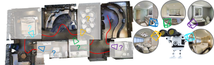
Figure 1: Environment Predictive Coding: During self-supervised learning, our model is given video walkthroughs of various 3D environments. We mask portions out of the trajectory (dotted lines) and learn to infer them from the unmasked parts (in red). We specifically mask out all overlapping views in a local neighborhood to limit the content shared with the unmasked views. The resulting EPC encoder builds environment-level representations of the seen content that are predictive of the unseen content (marked with a “?”), conditioned on the camera poses. The agent then uses this learned encoder in multiple navigational tasks in novel environments.

To this end, we devise a self-supervised zone prediction task in which the model learns environment embeddings by watching egocentric view sequences from other agents navigating in 3D environments in pre-collected videos. Specifically, we segment each video into zones of visually and geometrically connected views, while ensuring limited overlap across zones in the same video. Then, we randomly mask out zones, and predict the masked views conditioned on both the unmasked zones’ views and the masked zones’ camera poses. Intuitively, to perform this task successfully, the model needs to reason about the geometry and semantics of the environment to figure out what is missing. We devise a transformer-based model to infer the masked visual features. Our general strategy can be viewed as a context prediction task in sequential data [15, 57, 28]—but, very differently, aimed at representing high-level semantic and geometric priors in 3D environments to aid embodied agents who act in them.

Through extensive experiments on Gibson and Matterport3D, we show that our method achieves good improvements on multiple navigation-oriented tasks compared to both state-of-the-art models and baselines that learn image-level embeddings.

2 Related work

Self-supervised visual representation learning: Prior work leverages self-supervision to learn image and video representations from large collections of unlabelled data. Image representations attempt proxy tasks such as inpainting [44] and instance discrimination [41, 11, 30], while video representation learning leverages signals such as temporal consistency [59, 18, 34] and contrastive predictions [28, 56]. The VideoBERT project [56, 57] jointly learns video and text representations from unannotated videos via filling in masked out information. Dense Predictive Coding [28, 29] learns video representations that capture the slow-moving semantics in videos. Whereas these methods focus on capturing human activity for video recognition, we aim to learn geometric and semantic cues in 3D spaces for embodied agents. Accordingly, unlike the existing video models [56, 57, 28], which simply infer missing frame features, our approach explicitly grounds its predictions in the 3D relationships between views.

Representation learning via auxiliary tasks for RL: Reinforcement learning approaches often suffer from high sample complexity, sparse rewards, and unstable training. Prior work tackles these challenges by using auxiliary tasks for learning image representations [39, 21, 37, 52, 66]. In contrast, we encode image sequences from embodied agents to obtain environment-level representations. Recent work also learns state representations via future prediction and implicit models [26, 16, 22, 27, 23]. In particular, neural rendering approaches achieve impressive reconstructions for arbitrary viewpoints [16, 36]. However, unlike our idea, they focus on pixelwise reconstruction, and their success has been limited to synthetically generated environments like DeepMind Lab [3]. In contrast to any of the above, we use egocentric videos to learn predictive feature encodings of photorealistic 3D environments to capture their naturally occurring regularities.

Scene completion: Past work in scene completion performs pixelwise reconstruction of 360 panoramas [32, 46], image inpainting [44], voxelwise reconstructions of 3D structures and semantics [53], and image-level extrapolation of depth and semantics [54, 65]. Recent work on visual navigation extrapolates maps of room-types [61, 40] and occupancy [45]. While our approach is also motivated by anticipating unseen elements, we learn to extrapolate in a high-dimensional feature space (rather than pixels, voxels, or semantic categories) and in a self-supervised manner without relying on human annotations. Further, the proposed model learns from egocentric video sequences captured by other agents, without assuming access to detailed scans of the full 3D environment as in past work.

Learning image representations for navigation: Prior work exploits ImageNet pretraining [24, 2, 10], mined object relations [64], video [6], and annotated datasets from various image tasks [51, 9] to aid navigation. While these methods also consider representation learning in the context of navigation tasks, they are limited to learning image-level functions for classification and proximity prediction. In contrast, we learn predictive representations for sequences of observations conditioned on the camera poses.

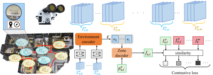
Figure 2: We propose the zone prediction task for self-supervised learning of environment embeddings from video walkthroughs generated by other agents. Each frame consists of the egocentric view and camera pose (top left). We group the frames in video $v$ into seen zones in cyan $\{Z_{s,0}^{v},\cdots,Z_{s,n}^{v}\}$ and unseen zones in yellow $\{Z_{u,0}^{v},\cdots,Z_{u,m}^{v}\}$ (top row). The zones are generated automatically based on viewpoint overlap in 3D space (bottom left). Given a camera pose $p_{u,i}^{v}$ sampled from the unseen zone $Z_{u,i}^{v}$, we use a transformer-based encoder-decoder architecture that generates environment embeddings $\mathcal{E}$ from the seen zones, and predicts the feature encoding $\hat{f}_{u,i}$ of $Z_{u,i}^{v}$ conditioned on the pose $p_{u,i}^{v}$ (bottom center). The model is trained to distinguish the positive $f_{u,i}^{v}$ from negatives in the same video $\{f_{u,j}^{v}\}_{j\neq i}$ as well from other videos $\{f_{k}^{w}\}_{t\neq s}$ (bottom right).

3 Approach

We propose environment predictive coding (EPC) to learn self-supervised environment-level representations (Sec. 3.1). To demonstrate the utility of these representations, we integrate them into a transformer-based navigation architecture and refine them for individual tasks (Sec. 3.2). As we will show in Sec. 4, our approach leads to both better performance and better sample efficiency compared to existing approaches.

3.1 Environment predictive coding

Our hypothesis is that it is valuable for an embodied agent to learn a predictive coding of the environment. The agent must not just encode the individual views it observes, but also learn to leverage the encoded information to anticipate the unseen parts of the environment. Our key idea is that the environment embedding must be predictive of unobserved content, conditioned on the agent’s camera pose. This equips an agent with the structural and semantic priors of 3D environments to quickly perform new tasks, like finding the refrigerator or covering more area.

We propose the proxy task of zone prediction to achieve this goal (see Fig. 2). For this task, we use a dataset of egocentric video walkthroughs collected in parallel by other agents deployed in various unseen environments (Fig. 2, top). For each video, we assume access to RGB-D, egomotion data, and camera intrinsics. Specifically, our current implementation uses egocentric camera trajectories from photorealistic scanned indoor environments (Gibson [63]) to sample the training videos; we leave leveraging in-the-wild consumer video as a challenge for future work.

We do not assume that the agents who generated those training videos were acting to address a particular navigation task. In particular, their behavior need not be tied to the downstream navigation-oriented tasks for which we test our learned representation. For example, a training video may show agents moving about to maximize their area coverage, or simply making naive forward-biased motions, whereas the encoder we learn is applicable to an array of navigation tasks (as we will demonstrate in Sec. 4). Furthermore, we assume that the environments seen in the videos are not accessible for interactive training. In practice, this means that we can collect data from different robots deployed in a large number of environments in parallel, without having to actually train our navigation policy on those environments. These assumptions are much weaker than those made by prior work on imitation learning and behavioral cloning that rely on task-specific data generated from experts [4, 20].

Our method works as follows. First, we automatically segment videos into “zones” which contain frames with significant view overlaps. We then perform the self-supervised zone prediction task on the segmented videos. Finally, we incorporate the learned environment encoder into an array of downstream navigation-oriented tasks. We explain each step in detail next.

Zone generation

At a glance, one might first consider masking arbitrary individual frames in the training videos. However, doing so is inadequate for representation learning, since unmasked frames having high viewpoint overlap with the masked frame can make its prediction trivial. Instead, our approach masks zones of frames at once. We define a zone to be a set of frames in the video which share a significant overlap in their viewpoints. We also require that the frames across multiple zones share little to no overlap.

To generate these zones, we first cluster frames in the videos based on the amount of pairwise-geometric overlap between views. We estimate the viewpoint overlap $\psi(o_{i},o_{j})$ between two frames $o_{i}$, $o_{j}$ by measuring their intersection in 3D point clouds obtained by backprojecting depth inputs into 3D space. See Appendix for more details. For a video of length $L$, we generate a distance matrix $D\in\mathbb{R}^{L\times L}$ where $D_{i,j}=1-\psi(o_{i},o_{j})$. We then perform hierarchical agglomerative clustering [38] to cluster the video frames into zones based on $D$ (see Fig. 2, bottom left). While these zones naturally tend to overlap near their edges, they typically capture disjoint sets of content in the video. Note that the zones segment video trajectories, not floorplan maps, since we do not assume access to the full 3D environment.

Zone prediction task

Having segmented the video into zones, we next present our EPC zone prediction task to learn environment embeddings (see Fig. 2). The main motivation in this task is to infer unseen zones in the video by previewing the global context spanning multiple seen zones. We randomly divide the video $v$ into seen zones $\{Z_{s,i}^{v}\}_{i=1}^{n}$ (cyan) and unseen zones $\{Z_{u,i}^{v}\}_{i=1}^{m}$ (yellow), where a zone $Z$ is a tuple of images and the corresponding camera poses $Z_{i}=\{(o_{j},p_{j})\}_{1}^{|Z_{i}|}$. Given the seen zones, and the camera pose from an unseen zone $p_{u,i}^{v}$, we need to infer a feature encoding of the unseen zone $Z_{u,i}^{v}$. To perform this task, we first extract visual features $x$ from each RGB-D frame $o$ in the video using pretrained CNNs (see Sec. 3.2). These features are concatenated with the corresponding pose $p$ and projected using an MLP $\mathcal{M}$ to obtain the image-level embedding. The target features for the unseen zone $Z_{u,i}^{v}$ are obtained by randomly sampling an image within the zone and extracting its camera pose and features:

$$f_{u,i}^{v}=\mathcal{M}([x,p]),\textrm{where }(x,p)\sim Z_{u,i}^{v}.$$ (1)

We use a transformer-based encoder-decoder model [58] to perform this task. Our model consists of an environment encoder and a zone decoder which infers the zone features (see Fig. 2, bottom). The environment encoder uses the image-level embeddings $\mathcal{M}([x,p])$ from the input zones and performs multi-headed self-attention to generate the environment embeddings $\mathcal{E}$.

The zone decoder attends to $\mathcal{E}$ using the camera pose from the unseen zone $p_{u,i}^{v}$ and predicts the zone features as follows:

$$\hat{f}_{u,i}=\textrm{ZoneDecoder}(\mathcal{E},p_{u,i}^{v}).$$ (2)

We transform all poses in the input zones relative to $p_{u,i}^{v}$ before encoding, which provides the model an egocentric view of the world. The environment encoder, zone decoder, and the projection function $\mathcal{M}$ are jointly trained using noise-contrastive estimation [25]. We use $\hat{f}_{u,i}$ as the anchor and $f_{u,i}^{v}$ from Eqn. 1 as the positive. We sample negatives from other unseen zones in the same video and from all zones in other videos. The loss for the $i^{\textrm{th}}$ unseen zone in video $v$ is:

where $\textrm{sim}(q,k)=\textrm{exp}\big{(}\frac{q\cdot k}{|q||k|}\frac{1}{\tau}\big{)}$ and $\tau$ is a temperature hyperparameter. The idea is to predict zone representations that are closer to the ground truth, while being sufficiently different from the negative zones. Since the unseen zones have only limited overlap with the seen zones, the model needs to effectively reason about the geometric and semantic context in the seen zones to differentiate the positive from the negatives. We discourage the model from simply capturing video-specific textures and patterns by sampling negatives from within the same video.

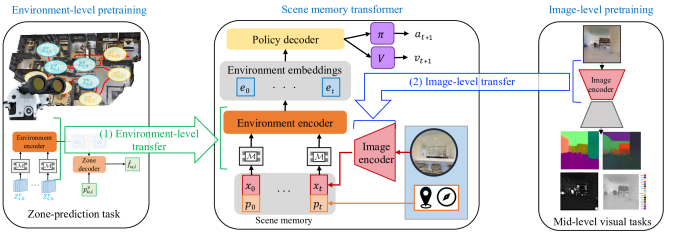
Figure 3: Integrating environment-level pre-training for navigation: Left: The first level of transfer occurs for the environment-level representations. We transfer the proposed EPC environment encoder and projection function $\mathcal{M}$ that are pre-trained for zone prediction. Right: The second level of transfer occurs for the image-level representations. We transfer a pre-trained MidLevel image encoder [51] to generate visual features for each input in the scene memory. Center: To train the SMT on a task, we keep the visual features frozen, and finetune the environment encoder and projection function $\mathcal{M}$ with the rest of the SMT model.

3.2 Environment embeddings for embodied agents

Having introduced our approach to learn environment embeddings in a self-supervised fashion, we now briefly overview how these embeddings are used for agents performing navigation-oriented tasks. To this end, we integrate our pre-trained environment encoder into the Scene Memory Transformer (SMT) [17]. Our choice of SMT is motivated by the recent successes of transformers in both NLP [15] and vision [57, 17]. However, our idea is potentially applicable to other forms of memory models as well.

We briefly overview the SMT architecture (see Fig. 3, center). It consists of a scene memory that stores visual features $\{x_{i}\}_{i=0}^{t}$ and agent poses $\{p_{i}\}_{i=0}^{t}$ generated from the observations seen during an episode. The environment encoder uses self-attention on the history of observations to generate a richer set of environment embeddings $\{e_{i}\}_{i=1}^{t}$. At a given time-step $t+1$, the policy decoder attends to the environment embeddings using the inputs $o_{t+1}$, which consist of the visual feature $x$ and agent pose $p$ at time $t+1$. The outputs of the policy decoder are used to sample an action $a_{t+1}$ and estimate the value $v_{t+1}$. We detail each component in the Appendix.

To incorporate our EPC environment embeddings, we modify two key components from the original SMT model. First, and most importantly, we initialize the environment encoder with our pre-trained EPC (see Fig. 3, left). Second, we replace the end-to-end trained image encoders with MidLevel features that are known to be useful across a variety of embodied tasks [51] (see Fig. 3, right). We consider two visual modalities as inputs: RGB and depth. For RGB, we extract features from the pre-trained models in the max-coverage set proposed by [51]. These include surface normals, keypoints, semantic segmentation, and 2.5D segmentation. For depth, we extract features from pre-trained models that predict surface normals and keypoints from depth [67]. For training the model on a navigation task, we keep the visual features frozen, and only finetune the environment encoder, policy decoder, policy $\pi$, and value function $V$.

4 Experiments

First, we review the experimental setup for the downstream navigation tasks (Sec. 4.1). Next, we detail the self-supervised learning setup and visualize the learned EPC embeddings (Sec. 4.2). We then evaluate the pre-trained EPC environment embeddings on multiple downstream tasks that require an embodied agent to move intelligently through an unmapped environment (Sec. 4.3). Finally, we evaluate the sensitivity of self-supervised learning to noise in the video data (Sec. 4.4), and assess noise robustness of the learned policies on downstream tasks (Sec. 4.5).

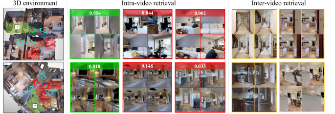
Figure 4: Each row shows one zone prediction example. Left: Top-down view of the 3D environment from which the video was sampled. The cyan viewing frusta correspond to the average pose for three input zones. Given the images and camera poses from each input zone, and a target camera pose (green frustum), the model predicts the corresponding zone feature (the masked green zone). Center: Given the inferred feature, we rank three masked (unobserved) zones from within the same video, where green is the positive zone and the red are the negatives. For each zone, we show four randomly sampled images along with the retrieval confidence. Our method retrieves the positive with high confidence. The model correctly predicts the existence of the narrow corridor (top row) and a kitchen counter (bottom row) given the target poses. Right: Top two retrieved zones from other videos that are closest to the inferred feature. The features predicted by the model are general enough to retrieve related concepts from other videos (narrow corridors and kitchens).

4.1 Experimental setup for downstream navigation

We perform experiments on the Habitat simulator [49] with Matterport3D (MP3D) [5] and Gibson [63], two challenging and photorealistic 3D datasets with $\sim 90$ and $500$ scanned real-world indoor environments, respectively. Our observation space consists of $171\times 128$ RGB-D observations and odometry sensor readings that provide the relative agent pose $p=(x,y,\theta)$ w.r.t the agent pose at $t=0$. Our action space consists of: move-forward by $25$\mathrm{c}\mathrm{m}$$, turn-left by $30^{\circ}$, and turn-right by $30^{\circ}$. For all methods, we assume noise-free actuation during training for simplicity. We evaluate with both noise-free and noisy sensing (pose, depth).

We use MP3D for interactive RL training, and reserve Gibson for evaluation. We use the default train/val/test split for MP3D [49] for 1000-step episodes. For Gibson, which has smaller environments, we evaluate on the $14$ validation environments for 500-step episodes. Following prior work [45, 8], we divide results on Gibson into small and large environments.

We evaluate our approach on three standard tasks from the literature:

1. Area coverage [10, 8, 47]: The agent is rewarded for maximizing the area covered (in $\mathrm{m}^{2}$) within a fixed time budget.
2. Flee [21]: The agent is rewarded for maximizing the flee distance (in $\mathrm{m}$), i.e., the geodesic distance between its starting location and the terminal location, for fixed-length episodes.
3. Object coverage [17, 47]: The agent is rewarded for maximizing the number of categories of objects covered during exploration (see Appendix). Since Gibson lacks extensive object annotations, we evaluate this task only on MP3D.

Together, these tasks capture different forms of geometric and semantic inference in 3D environments (e.g., area/object coverage encourage finding large open spaces/new objects, respectively). We compare our approach to the following baselines:
Scratch baselines: We randomly initialize the visual encoders and policy and train them end-to-end for each task. Images are encoded using ResNet-18. Agent pose and past actions are encoded using FC layers. These are concatenated to obtain the features at each time step. We use three temporal aggregation schemes. Reactive (scratch) has no memory. RNN (scratch) uses a 2-layer LSTM as the temporal memory. SMT (scratch) uses a Scene Memory Transformer for aggregating observations [17].
SMT (MidLevel): extracts image features from pre-trained encoders that solve various mid-level perceptual tasks [51]. This is an ablation of our model from Sec. 3.2 that uses the same image features, but randomly initializes the environment encoder. This SoTA image-level encoder is a critical baseline to show the impact of our proposed EPC environment-level encoder.
SMT (Video): Inspired by Dense Predictive Coding [28], this baseline uses MidLevel features and pre-trains the environment encoder as a video-level model using the same training videos as our model. It uses 25 consecutive frames as inputs and predicts the features sampled from the next 15 frames (following timespans used in prior work [28]). We mask out the camera poses in the inputs and query based on the time (not pose). We train the model using the NCE loss in Eqn. 3.
OccupancyMemory: This is similar to the SoTA Active Neural SLAM model [8] that maximizes area coverage, but upgraded to use ground-truth depth to build the map (instead of RGB) and a state-of-the-art PointNav agent [60] for low-level navigation (instead of a planner). It represents the environment as a top-down occupancy map.

All models are trained in PyTorch [43] with DD-PPO [60] for 15M frames with 64 parallel processes and the Adam optimizer. See Appendix.

	Area coverage (m2)			Flee (m)			Object coverage (#obj)
Method	Gibson-S	Gibson-L	MP3D	Gibson-S	Gibson-L	MP3D	MP3D-cat.	MP3D-inst.
Reactive (scratch)	$17.4\pm 0.2$	$22.8\pm 0.6$	$68.0\pm 1.3$	$1.9\pm 0.1$	$2.5\pm 0.3$	$5.1\pm 0.3$	$6.2\pm 0.0$	$19.0\pm 0.2$
RNN (scratch)	$20.6\pm 0.4$	$28.6\pm 0.3$	$79.0\pm 2.0$	$2.3\pm 0.2$	$2.8\pm 0.4$	$5.8\pm 0.0$	$6.0\pm 0.0$	$18.6\pm 0.2$
SMT (scratch)	$23.0\pm 0.6$	$32.3\pm 0.8$	$104.8\pm 2.2$	$3.2\pm 0.2$	$4.4\pm 0.4$	$6.9\pm 0.6$	$7.0\pm 0.2$	$23.2\pm 0.9$
SMT (MidLevel)	$29.1\pm 0.1$	$47.2\pm 1.6$	$155.6\pm 2.0$	$4.2\pm 0.0$	$6.0\pm 0.4$	$10.6\pm 0.3$	$7.6\pm 0.2$	$26.8\pm 0.6$
SMT (Video)	$28.8\pm 0.4$	$47.6\pm 2.4$	$141.2\pm 4.4$	$4.0\pm 0.0$	$6.5\pm 0.4$	$10.8\pm 0.6$	$7.5\pm 0.1$	$26.0\pm 0.2$
OccupancyMemory	$29.4\pm 0.0$	$\bm{67.4}\pm 0.9$	$155.6\pm 1.4$	$2.8\pm 0.0$	$7.0\pm 0.4$	$\bm{14.1}\pm 0.6$	$7.8\pm 0.1$	$27.8\pm 0.4$
EPC	$\bm{31.5}\pm 0.1$	$62.2\pm 1.0$	$\bm{172.4}\pm 0.6$	$\bm{4.4}\pm 0.0$	$\bm{8.0}\pm 0.4$	$12.6\pm 0.2$	$\bm{9.0}\pm 0.0$	$\bm{36.4}\pm 1.0$

Table 1: Downstream task performance at the end of the episode. Gibson-S/L means small/large. MP3D-cat./inst. means categories/instances. All methods are evaluated on three random seeds. Here EPC uses video walkthroughs collected by an exploration agent that maximizes its area coverage. See Appendix for performance vs. time step plots.

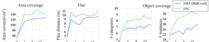
Figure 5: Sample efficiency on Matterport3D val split. Our environment-level pre-training leads to 4-8$\times$ training sample efficiency when compared to SoTA image-level pre-training. See Appendix for Gibson plots.

4.2 Self-supervised learning with EPC

We generate walkthroughs for self-supervised learning from $332$ Gibson training environments. Note that these environments are not accessible to the RL agent for interactive training.

We collect the video data using two policies: 1) an SMT (scratch) agent that was trained to perform area-coverage on MP3D, and 2) a heuristic navigation agent that moves forward until colliding, then turns (cf. Sec. 4.4). We test the impact of each video source separately below.

In both cases, the agents explore each Gibson environment starting from multiple locations and gather the RGB-D and odometer readings for 500 steps per video. This results in $\sim$5,000 videos per agent, which we divide into an 80-20 train/val split. We use these videos to pre-train environment encoders on the EPC zone prediction task for 50 epochs. The hyperparameters are provided in Appendix D. We qualitatively analyze the masked zone prediction results from EPC in Fig. 4.

4.3 Downstream task performance

Now we transfer these features to downstream navigation tasks. Tab. 1 shows the results. On both datasets, we observe the following ordering:

$$\textrm{Reactive (scratch)}~{}<~{}\textrm{RNN (scratch)}~{}<~{}\textrm{SMT (scratch)}.$$ (4)

This is in line with results reported by [17] and verifies our implementation of SMT. Using MidLevel features for SMT leads to significant gains in performance versus training image encoders from scratch.

Environment Predictive Coding (EPC) effectively combines environment-level and image-level pretraining to provide substantial improvements compared to only image-level pretraining from SMT (MidLevel), particularly for larger environments. Furthermore, SMT (Video)—the video-level pre-training strategy—significantly underperforms EPC, as it ignores the underlying spatial information during self-supervised learning. This highlights EPC’s value in representing the underlying 3D spaces of the walkthroughs instead of treating them simply as video frames. EPC also competes closely and even slightly outperforms the state-of-the-art OccupancyMemory on the geometric tasks area coverage and flee, while providing a significant gain on object coverage. Thus, our model competes strongly with the purely geometric representation model on the tasks that the latter was designed for, while outperforming it significantly on the semantic task. Note that OccupancyMemory performs poorly on Flee in Gibson-S since its goal sampling strategy is biased towards larger environments. See Appendix H.

Finally, in Fig. 5, we can see that environment-level pre-training from EPC offers significantly higher sample efficiency: our method reaches the best performance of SMT (MidLevel) 4-8$\times$ faster. This advantage persists even after accounting for the $\sim$2M frames of off-policy experience in the video data (see Tab. 4). This confirms our hypothesis: transferring environment-level representations learned via contextual reasoning can help embodied agents learn faster compared to the current approach of transferring image-level encoders alone.

	Area coverage (m2)			Flee (m)			Object coverage (#obj)
Method	Gibson-S	Gibson-L	MP3D	Gibson-S	Gibson-L	MP3D	MP3D-cat.	MP3D-inst.
SMT (MidLevel)	$29.1\pm 0.1$	$47.2\pm 1.7$	$155.7\pm 2.0$	$4.2\pm 0.0$	$6.0\pm 0.4$	$10.6\pm 0.3$	$7.6\pm 0.1$	$26.8\pm 0.6$
EPC	$31.5\pm 0.1$	$62.2\pm 1.0$	$172.5\pm 0.6$	$4.5\pm 0.0$	$8.0\pm 0.5$	$12.7\pm 0.2$	$\bm{9.0}\pm 0.1$	$36.4\pm 1.0$
EPC w/ noisy depth	$31.4\pm 0.4$	$60.5\pm 1.4$	$171.3\pm 5.0$	$4.2\pm 0.1$	$7.6\pm 1.0$	$11.5\pm 0.5$	$8.6\pm 0.1$	$35.2\pm 0.6$
EPC w/ noisy depth and pose	$\bm{32.2}\pm 0.1$	$63.6\pm 3.2$	$\bm{181.0}\pm 1.5$	$\bm{4.9}\pm 0.2$	$7.9\pm 0.2$	$13.3\pm 0.4$	$8.5\pm 0.2$	$33.8\pm 1.2$
EPC w/ heuristic video policy	$31.4\pm 0.3$	$61.6\pm 2.3$	$176.4\pm 4.8$	$4.5\pm 0.2$	$7.1\pm 0.4$	$12.3\pm 0.4$	$8.5\pm 0.1$	$35.9\pm 0.1$

Table 2: Impact of noisy video data (corrupted pose and/or depth) and a simple heuristic policy for video generation on EPC self-supervised learning. EPC maintains its advantage over the SMT (MidLevel) which randomly initializing the environment encoders.

	Area coverage (m2)			Flee (m)			Object cov. (#cat.)
Method	NF	N-D	N-D,P	NF	N-D	N-D,P	NF	N-D	N-D,P
SMT (MidLevel)	$155.7\pm 2.0$	$145.1\pm 2.3$	$134.2\pm 1.8$	$10.6\pm 0.3$	$10.6\pm 0.6$	$10.8\pm 0.4$	$7.6\pm 0.2$	$7.3\pm 0.1$	$7.3\pm 0.2$
OccupancyMemory	$155.6\pm 1.4$	$86.6\pm 2.2$	$85.2\pm 2.4$	$\bm{14.1}\pm 0.6$	$10.9\pm 0.2$	$10.2\pm 0.3$	$7.8\pm 0.1$	$5.8\pm 0.0$	$5.8\pm 0.0$
EPC	$\bm{172.5}\pm 0.6$	$\bm{161.6}\pm 3.1$	$\bm{159.3}\pm 2.0$	$12.7\pm 0.2$	$\bm{12.0}\pm 0.8$	$\bm{12.0}\pm 0.1$	$\bm{9.0}\pm 0.1$	$\bm{8.5}\pm 0.1$	$\bm{8.5}\pm 0.3$

Table 3: Comparing robustness to sensor noise on downstream tasks in Matterport3D. Note: NF denotes noise free sensing, N-D denotes noisy depth (and noise-free pose), and N-D,P denotes noisy depth and pose. See Appendix G for full results.

4.4 Sensitivity analysis of self-supervised learning

Next we analyze the sensitivity of EPC to 1) sensory noise in the videos and 2) the exploration strategy used for video data collection. Specifically, we inject noise in the depth and pose data from the walkthrough videos using existing noise models from [13] and [45]. The depth noise model combines disparity-based quantization, high-frequency noise, and low-frequency distortion [13]. The odometry noise is based on data collected from a LoCoBot robot [45, 8]. We also replace the video walkthroughs from the area-coverage agent with an equivalent amount of data collected by a simple heuristic used in prior work [10, 47]. The heuristic instructs the video agent to move as follows: move forward until colliding, then turn left or right by a random amount, then continue moving forward.

Tab. 2 shows the impact of each of these changes on the downstream task performance. For reference, we compare these with random initilization of the environment encoder in SMT (MidLevel). Our approach EPC is reasonably robust to changes in the video data during SSL training. The performance remains stable when noise is injected into depth inputs. While it starts to decline on object coverage when we further inject noise into the pose inputs, EPC still retains its advantages over SMT (MidLevel). Note that we do not employ any noise-correction mechanisms, which could better limit this decline [8, 45]. Finally, the performance is not significantly impacted when we use video data from the simple exploration heuristic, emphasizing that EPC does not require a strong exploration policy for the agent that generates the self-supervised training videos, nor does it require a tight similarity between the tasks demonstrated in the videos and the downstream tasks.

	Area coverage (m2)			Flee (m)			Object coverage (#obj)
Method	Gibson-S	Gibson-L	MP3D	Gibson-S	Gibson-L	MP3D	MP3D-cat.	MP3D-inst.
SMT (Video) @ 15M	$28.8\pm 0.4$	$47.6\pm 2.4$	$141.2\pm 4.4$	$4.0\pm 0.0$	$6.5\pm 0.4$	$10.8\pm 0.6$	$7.5\pm 0.1$	$26.0\pm 0.2$
SMT (Video) @ 13M	$28.4\pm 0.3$	$44.7\pm 2.5$	$126.2\pm 3.4$	$3.7\pm 0.1$	$4.9\pm 0.2$	$10.0\pm 0.5$	$7.2\pm 0.1$	$24.3\pm 0.6$
EPC @ 15M	$\bm{31.5}\pm 0.1$	$62.2\pm 1.0$	$172.4\pm 0.6$	$4.4\pm 0.0$	$\bm{8.0}\pm 0.4$	$12.6\pm 0.2$	$\bm{9.0}\pm 0.0$	$\bm{36.4}\pm 1.0$
EPC @ 13M	$31.2\pm 0.2$	$\bm{64.0}\pm 0.5$	$\bm{176.3}\pm 3.8$	$\bm{4.6}\pm 0.2$	$7.1\pm 0.8$	$\bm{13.8}\pm 0.7$	$\bm{9.0}\pm 0.0$	$\bm{36.4}\pm 1.0$

Table 4: Offsetting on-policy interaction with video-level experience: Each walkthrough video contains $\sim$500 frames and the dataset contains $\sim$2M frames. While this is off-policy walkthrough data used only for representation learning, we nonetheless re-evaluate the checkpoints of “EPC” and “SMT (Video)” before 15M-2M = 13M frames to account for the additional observations from the video data. The performance at 13M and 15M frames remains similar for EPC, whereas it decreases at 13M frames for SMT (Video). Thus, EPC maintains its advantages over the best baselines from Tab. 1 after accounting for any additional experience from the video walkthroughs.

4.5 Robustness of learned policies to sensor noise

In the previous experiments, we assume the availability of ground-truth depth and pose sensors for downstream tasks (Tab. 2 added pose and depth noise to the walkthrough videos only). Now, we relax these assumptions and re-evaluate all methods by injecting noise in the depth and pose sensors for downstream tasks (same noise models from prior work that we applied in Sec. 4.4), without any noise-correction. This is a common evaluation protocol for assessing noise robustness [10, 47]. We compare the top three methods on MP3D in Tab. 3 and provide the complete set of results in Appendix G. As expected, the performance declines slightly as we add noise to more sensors (depth, then pose). However, most approaches are reasonably stable. EPC outperforms all methods when all noise sources are added. OccupancyMemory declines rapidly in the absence of noise-correction due to accumulated errors in the map.

5 Conclusions

We introduced Environment Predictive Coding, a self-supervised approach to learn environment-level representations for embodied agents. By training on video walkthroughs generated by other agents, our model learns to infer missing content through a zone-prediction task. When transferred to multiple downstream embodied agent tasks, the resulting embeddings lead to better performance and sample efficiency compared to the current practice of transferring only image-level representations. In future work, we plan to extend our idea for goal-driven tasks like PointNav and ObjectNav.

Appendix

Appendix A Zone generation

As discussed in the main paper, we generate zones by first clustering frames in the video based on their geometric overlap. Here, we provide details on how this overlap is estimated. First, we project pixels in the image to 3D point-clouds using the camera intrinsics and the agent pose. Let $D_{i}$, $p_{i}$ be the depth map and agent pose for frame $i$ in the video. The agent’s pose in frame $i$ can be expressed as $p_{i}=(\bm{R}_{i},\bm{t}_{i})$, with $\bm{R}_{i},\bm{t}_{i}$ representing the agent’s camera rotation and translation in the world coordinates. Let $\bm{K}\in\mathbb{R}^{3\times 3}$ be the intrinsic camera matrix, which is assumed to be provided for each video. We then project each pixel $x_{ij}$ in the depth map $D_{i}$ to the 3D point cloud as follows:

$$w_{ij}=\begin{bmatrix}\bm{R}_{i}&\bm{t}_{i}\\ \bm{0}&1\end{bmatrix}\bm{K}^{-1}x_{ij},~{}\forall j\in\{1,...,S_{i}\}$$ (5)

where $S_{i}$ is the total number of pixels in $D_{i}$. By doing this operation for each pixel, we can obtain the point-cloud $\bm{W}_{i}$ corresponding to the depth map $D_{i}$. To compute the geometric overlap between two frames $i$ and $j$, we estimate the overlap in their point-clouds $\bm{W}_{i}$ and $\bm{W}_{j}$. Specifically, for each point $w_{i}\in\bm{W}_{i}$, we retrieve the nearest neighbor from $w_{j}\in\bm{W}_{j}$ and check whether the pairwise distance in 3D space is within a threshold $\tau$: $||w_{i}-w_{j}||_{2}<\tau$ . If this condition is satisfied, then a match exists for $w_{i}$. Then, we define the overlap fraction $\psi(D_{i},D_{j})$ the fraction of points in $\bm{W}_{i}$ which have a match in $\bm{W}_{j}$. This overlap fraction is computed pairwise between all frames in the video, and hierarchical agglomerative clustering is performed using this similarity measure.

Appendix B Task details

For the object coverage task, to determine if an object is covered, we check if it is within $3$\mathrm{m}$$ of the agent, present in the agent’s field of view, and if it is not occluded [47]. We use a shaped reward function:

$$R_{t}=O_{t}-O_{t-1}+0.02(C_{t}-C_{t-1}),$$ (6)

where $O_{t}$, $C_{t}$ are the number of object categories and 2D grid-cells visited by time $t$ (similar to  [17]).

Appendix C Scene memory transformer

We provide more details about individual components of the Scene Memory Transformer [17]. As discussed in the main paper, the SMT model consists of a scene memory for storing the visual features $\{x_{i}\}_{i=0}^{t}$ and agent poses $\{p_{i}\}_{i=0}^{t}$ seen during an episode. The environment encoder uses self-attention on the scene memory to generate a richer set of environment embeddings $\{e_{i}\}_{i=1}^{t}$. The policy decoder attends to the environment embeddings using the inputs $o_{t+1}$, which consist of the visual feature $x$, and agent pose $p$ at time $t+1$. The outputs of the policy decoder are used to sample an action $a_{t+1}$ and estimate the value $v_{t+1}$. Next, we discuss the details of the individual components.

Scene memory

It stores the visual features derived from the input images and the agent poses at each time-step. Motivated by the ideas from [51], we use mid-level features derived from various pre-trained CNNs for each input modality. In this work, we consider two input modalities: RGB, and depth. For RGB inputs, we extract features from the pre-trained models in the max-coverage set proposed in [51]. These include surface normals, keypoints, semantic segmentation, and 2.5D segmentation. For depth inputs, we extract features from pre-trained models that predict surface normals and keypoints from depth [67]. For simplicity, we assume that the ground-truth pose is available to the agent in the form of $(x_{t},y_{t},z_{t},\theta_{t})$ at each time-step, where $\theta_{t}$ is the agent heading. While this can be relaxed by following ideas from state-of-the-art approaches to Neural SLAM [8, 45], we reserve this for future work as it is orthogonal to our primary contributions.

Attention mechanism

Following the notations from [58], we define the attention mechanism used in the environment encoder and policy decoder. Given two inputs $X\in\mathbb{R}^{n_{1}\times d_{x}}$ and $Y\in\mathbb{R}^{n_{2}\times d_{y}}$, the attention mechanism attends to $Y$ using $X$ as follows:

$$\textrm{Attn}(X,Y)=\textrm{softmax}\bigg{(}\frac{Q_{X}K_{Y}^{T}}{\sqrt{d_{k}}}\bigg{)}V_{Y}$$ (7)

where $Q_{X}\in\mathbb{R}^{n_{1}\times d_{k}},K_{Y}\in\mathbb{R}^{n_{2}\times d_{k}},V_{Y}\in\mathbb{R}^{n_{2}\times d_{v}}$ are the queries, keys, and values computed from $X$ and $Y$ as follows: $Q_{X}=XW^{q}$, $K_{Y}=YW^{k}$, and $V_{Y}=YW^{v}$. $W^{q},W^{k},W^{v}$ are learned weight matrices. The multi-headed version of Attn generates multiple sets of queries, keys, and values to obtain the attended context $C\in\mathbb{R}^{n_{1}\times d_{v}}$.

$$\textrm{MHAttn}(X,Y)=\textrm{FC}([\textrm{Attn}^{h}(X,Y)]_{h=1}^{H}).$$ (8)

We use the transformer implementation from PyTorch [43]. Here, the multi-headed attention block builds on top of MHAttn by using residual connections, LayerNorm (LN) and fully connected (FC) layers to further encode the inputs.

$$\begin{gathered}\textrm{MHAttnBlock}(X,Y)=\textrm{LN}(\textrm{MLP}(H)+H)\end{gathered}$$ (9)

where $H=\textrm{LN}(\textrm{MHAttn}(X,Y)+X)$, and MLP has 2 FC layers with ReLU activations. The environment encoder performs self-attention between the features stored in the scene memory to obtain the environment encoding $E$.

$$E=\textrm{EnvironmentEncoder}(M)=\textrm{MHAttnBlock}(M,M).$$ (10)

The policy decoder attends to the environment encodings $E$ using the current observation $x_{t},p_{t}$.

$$\textrm{PolicyDecoder}([x_{t},p_{t}],E)=\textrm{MHAttnBlock}(\textrm{FC}([x_{t},p_{t}]),E)$$ (11)

We transform the pose vectors $\{p_{i}\}_{i=1}^{n}$ from the scene memory relative to the current agent pose $p_{t}$ as this allows the agent to maintain an egocentric view of past inputs [17].

Appendix D Hyperparameters

We detail the list of hyperparameter choices for different tasks and models in Tab. 5. For SMT (Video), we randomly sample 40 consecutive frames in the video and predict the final 15 frames from the initial 25 frames (based on Dense Predictive Coding [28]). For EPC, we randomly mask out 4 zones in the video and predict them from the remaining video. The hyperparameters are selected based on validation performance on the downstream tasks.

RL Optimization
Optimizer	Adam
Learning rate	0.00025 - 0.001
$\#$ parallel actors	64
PPO mini-batches	2
PPO epochs	2
PPO clip param	0.2
Value loss coefficient	0.5
Entropy coefficient	0.01
Advantage estimation	GAE
Normalized advantage?	Yes
Training episode length	1000
GRU history length	128
$\#$ training steps (in millions)	15
RNN hyperparameters
Hidden size	128
RNN type	LSTM
Num recurrent layers	2
SMT hyperparameters
Hidden size	128
Scene memory length	500
$\#$ attention heads	8
$\#$ encoder layers	1
$\#$ decoder layers	1
Occupancy memory hyperparameters
Action space range	$48$\mathrm{m}$\times 48$\mathrm{m}$$
$\#$ global action sampling interval	$25$
Reward scaling factors for different tasks
Task	Reward scale
Area coverage	0.3
Flee	1.0
Object coverage	1.0
Self-supervised learning optimization
Optimizer	Adam
Learning rate	0.0001
Video batch size	20
Temperature ($\tau$)	0.1

Table 5: Hyperparameters for training our RL and self-supervised learning models.

Appendix E Downstream task performance vs. time

We show the downstream task performance as a function of time in Fig. 6. We evaluate each model with 3 different random seeds and report the mean and the $95\%$ confidence interval in the plots.

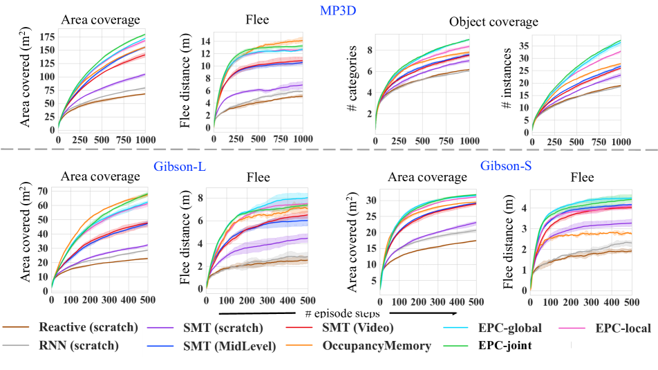
Figure 6: We highlight the downstream task performance as a function of episode time on both Matterport3D and Gibson.

Appendix F Sample efficiency curves on Gibson

We plot the Gibson validation performance as a function of training experience in Fig. 7. EPC achieves better sample efficiency through environment-level pre-training when compared to the image-level pre-training baseline SMT (MidLevel).

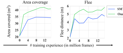
Figure 7: Sample efficiency on Gibson val split. Our environment-level pre-training leads to 4-8$\times$ training sample efficiency when compared to SoTA image-level pre-training.

Appendix G Complete analysis of noise robustness in downstream tasks

In Tab. 3 from the main paper, we compared the noise robustness of top three approaches on MP3D. Here, we present the complete set of results for all methods on Gibson and MP3D in Tab. 6.

	Matterport3D
	Area coverage (m2)			Flee (m)			Object cov. (#cat.)
Method	NF	N-D	N-D,P	NF	N-D	N-D,P	NF	N-D	N-D,P
Reactive (scratch)	$68.0\pm 1.3$	$65.8\pm 1.4$	$65.7\pm 1.5$	$5.1\pm 0.3$	$5.3\pm 0.2$	$5.3\pm 0.2$	$6.2\pm 0.0$	$6.0\pm 0.0$	$6.0\pm 0.0$
RNN (scratch)	$79.0\pm 2.0$	$74.0\pm 0.8$	$73.4\pm 1.3$	$5.9\pm 0.0$	$5.9\pm 0.3$	$6.0\pm 0.2$	$6.0\pm 0.0$	$5.9\pm 0.0$	$5.9\pm 0.0$
SMT (scratch)	$104.8\pm 2.2$	$101.6\pm 0.9$	$99.2\pm 2.9$	$6.9\pm 0.6$	$6.6\pm 0.2$	$7.4\pm 0.2$	$7.0\pm 0.2$	$6.8\pm 0.1$	$6.7\pm 0.1$
SMT (MidLevel)	$155.7\pm 2.0$	$145.1\pm 2.3$	$134.2\pm 1.8$	$10.6\pm 0.3$	$10.6\pm 0.6$	$10.8\pm 0.4$	$7.6\pm 0.2$	$7.3\pm 0.1$	$7.3\pm 0.2$
SMT (Video)	$141.2\pm 4.5$	$129.2\pm 2.1$	$125.8\pm 2.6$	$10.8\pm 0.6$	$10.0\pm 0.4$	$9.6\pm 0.1$	$7.5\pm 0.1$	$7.4\pm 0.0$	$7.4\pm 0.0$
OccupancyMemory	$155.6\pm 1.4$	$86.6\pm 2.2$	$85.2\pm 2.4$	$\bm{14.1}\pm 0.6$	$10.9\pm 0.2$	$10.2\pm 0.3$	$7.8\pm 0.1$	$5.8\pm 0.0$	$5.8\pm 0.0$
EPC	$\bm{172.5}\pm 0.6$	$\bm{161.6}\pm 3.1$	$\bm{159.3}\pm 2.0$	$12.7\pm 0.2$	$\bm{12.0}\pm 0.8$	$\bm{12.0}\pm 0.1$	$\bm{9.0}\pm 0.1$	$\bm{8.5}\pm 0.1$	$\bm{8.5}\pm 0.3$
	Gibson-S
	Area coverage (m2)			Flee (m)			Object cov. (#cat.)
Method	NF	N-D	N-D,P	NF	N-D	N-D,P	NF	N-D	N-D,P
Reactive (scratch)	$17.4\pm 0.2$	$17.8\pm 0.4$	$17.8\pm 0.4$	$1.9\pm 0.1$	$1.8\pm 0.1$	$1.8\pm 0.1$	-	-	-
RNN (scratch)	$20.6\pm 0.4$	$21.5\pm 0.3$	$21.6\pm 0.2$	$2.3\pm 0.2$	$2.2\pm 0.2$	$2.2\pm 0.2$	-	-	-
SMT (scratch)	$23.0\pm 0.7$	$23.5\pm 0.4$	$23.4\pm 0.4$	$3.3\pm 0.2$	$3.3\pm 0.0$	$2.8\pm 0.1$	-	-	-
SMT (MidLevel)	$29.1\pm 0.1$	$30.8\pm 0.4$	$30.8\pm 0.6$	$4.2\pm 0.0$	$4.1\pm 0.0$	$3.4\pm 0.0$	-	-	-
SMT (Video)	$28.8\pm 0.4$	$30.8\pm 0.4$	$30.7\pm 0.4$	$4.0\pm 0.0$	$3.9\pm 0.0$	$3.4\pm 0.1$	-	-	-
OccupancyMemory	$29.4\pm 0.0$	$30.8\pm 0.3$	$30.6\pm 0.2$	$2.8\pm 0.0$	$3.1\pm 0.0$	$3.0\pm 0.2$	-	-	-
EPC	$\bm{31.5}\pm 0.1$	$\bm{34.0}\pm 0.2$	$\bm{34.0}\pm 0.2$	$\bm{4.5}\pm 0.0$	$\bm{4.6}\pm 0.2$	$\bm{4.4}\pm 0.1$	-	-	-
	Gibson-L
	Area coverage (m2)			Flee (m)			Object cov. (#cat.)
Method	NF	N-D	N-D,P	NF	N-D	N-D,P	NF	N-D	N-D,P
Reactive (scratch)	$22.8\pm 0.6$	$22.4\pm 0.2$	$22.4\pm 0.2$	$2.5\pm 0.3$	$2.6\pm 0.4$	$2.6\pm 0.4$	-	-	-
RNN (scratch)	$28.6\pm 0.3$	$27.9\pm 2.4$	$28.2\pm 2.5$	$2.8\pm 0.4$	$2.7\pm 0.4$	$2.8\pm 0.4$	-	-	-
SMT (scratch)	$32.3\pm 0.8$	$33.4\pm 1.2$	$32.6\pm 1.9$	$4.4\pm 0.4$	$4.6\pm 0.2$	$4.4\pm 0.1$	-	-	-
SMT (MidLevel)	$47.2\pm 1.6$	$49.2\pm 0.4$	$46.8\pm 2.8$	$6.0\pm 0.4$	$5.4\pm 0.4$	$5.1\pm 0.6$	-	-	-
SMT (Video)	$47.6\pm 2.4$	$48.3\pm 1.5$	$48.0\pm 1.0$	$6.5\pm 0.4$	$6.0\pm 0.3$	$4.8\pm 0.4$	-	-	-
OccupancyMemory	$\bm{67.4}\pm 0.9$	$56.8\pm 0.8$	$56.9\pm 0.8$	$7.0\pm 0.4$	$6.9\pm 0.4$	$6.9\pm 0.3$	-	-	-
EPC	$62.2\pm 1.0$	$\bm{66.7}\pm 1.5$	$\bm{64.2}\pm 1.8$	$\bm{8.0}\pm 0.5$	$\bm{8.2}\pm 1.0$	$\bm{8.2}\pm 0.6$	-	-	-

Table 6: Comparing robustness to sensor noise on downstream tasks in Gibson and Matterport3D. Note: NF denotes noise free sensing, N-D denotes noisy depth (and noise-free pose), and N-D,P denotes noisy depth and pose.

Appendix H OccupancyMemory performance on Flee

OccupancyMemory relies on a global policy that samples a spatial goal location for navigation. A local navigation policy [60] then executes a series of low-level actions to reach that goal. Our qualitative analyses indicate that the global policy overfit to large MP3D environments. It often samples far away exploration targets, relying on the local navigator to explore the spaces along the sampled direction. However, this strategy fails in the small Gibson-S environments (typically a single room). Selecting far away targets results in the local navigator oscillating in place trying to exit a single-room environment. This does not affect area coverage much because it suffices to stand in the middle of a small room and look at all sides.

References

- [1] Peter Anderson, Qi Wu, Damien Teney, Jake Bruce, Mark Johnson, Niko Sünderhauf, Ian Reid, Stephen Gould, and Anton van den Hengel. Vision-and-language navigation: Interpreting visually-grounded navigation instructions in real environments. In Proceedings of the IEEE Conference on Computer Vision and Pattern Recognition (CVPR), 2018.
- [2] Peter Anderson, Qi Wu, Damien Teney, Jake Bruce, Mark Johnson, Niko Sünderhauf, Ian Reid, Stephen Gould, and Anton van den Hengel. Vision-and-language navigation: Interpreting visually-grounded navigation instructions in real environments. In Proceedings of the IEEE Conference on Computer Vision and Pattern Recognition, pages 3674–3683, 2018.
- [3] Charles Beattie, Joel Z. Leibo, Denis Teplyashin, Tom Ward, Marcus Wainwright, Heinrich Küttler, Andrew Lefrancq, Simon Green, Víctor Valdés, Amir Sadik, Julian Schrittwieser, Keith Anderson, Sarah York, Max Cant, Adam Cain, Adrian Bolton, Stephen Gaffney, Helen King, Demis Hassabis, Shane Legg, and Stig Petersen. Deepmind lab. CoRR, abs/1612.03801, 2016.
- [4] Mariusz Bojarski, Davide Del Testa, Daniel Dworakowski, Bernhard Firner, Beat Flepp, Prasoon Goyal, Lawrence D Jackel, Mathew Monfort, Urs Muller, Jiakai Zhang, et al. End to end learning for self-driving cars. arXiv preprint arXiv:1604.07316, 2016.
- [5] Angel Chang, Angela Dai, Tom Funkhouser, Matthias Nießner, Manolis Savva, Shuran Song, Andy Zeng, and Yinda Zhang. Matterport3d: Learning from rgb-d data in indoor environments. In Proceedings of the International Conference on 3D Vision (3DV), 2017. MatterPort3D dataset license available at: http://kaldir.vc.in.tum.de/matterport/MP_TOS.pdf.
- [6] Matthew Chang, Arjun Gupta, and Saurabh Gupta. Semantic visual navigation by watching youtube videos. arXiv preprint arXiv:2006.10034, 2020.
- [7] Devendra Singh Chaplot, Dhiraj Gandhi, Abhinav Gupta, and Ruslan Salakhutdinov. Object goal navigation using goal-oriented semantic exploration. arXiv preprint arXiv:2007.00643, 2020.
- [8] Devendra Singh Chaplot, Saurabh Gupta, Dhiraj Gandhi, Abhinav Gupta, and Ruslan Salakhutdinov. Learning to explore using active neural mapping. 8th International Conference on Learning Representations, ICLR 2020, 2020.
- [9] Devendra Singh Chaplot, Ruslan Salakhutdinov, Abhinav Gupta, and Saurabh Gupta. Neural topological slam for visual navigation. In Proceedings of the IEEE/CVF Conference on Computer Vision and Pattern Recognition, pages 12875–12884, 2020.
- [10] Tao Chen, Saurabh Gupta, and Abhinav Gupta. Learning exploration policies for navigation. In 7th International Conference on Learning Representations, ICLR 2019, 2019.
- [11] Ting Chen, Simon Kornblith, Mohammad Norouzi, and Geoffrey Hinton. A simple framework for contrastive learning of visual representations. arXiv preprint arXiv:2002.05709, 2020.
- [12] Ricson Cheng, Ziyan Wang, and Katerina Fragkiadaki. Geometry-aware recurrent neural networks for active visual recognition. In Advances in Neural Information Processing Systems, pages 5081–5091, 2018.
- [13] Sungjoon Choi, Qian-Yi Zhou, and Vladlen Koltun. Robust reconstruction of indoor scenes. In Proceedings of the IEEE Conference on Computer Vision and Pattern Recognition, pages 5556–5565, 2015.
- [14] Abhishek Das, Samyak Datta, Georgia Gkioxari, Stefan Lee, Devi Parikh, and Dhruv Batra. Embodied question answering. In Proceedings of the IEEE Conference on Computer Vision and Pattern Recognition Workshops, pages 2054–2063, 2018.
- [15] Jacob Devlin, Ming-Wei Chang, Kenton Lee, and Kristina Toutanova. Bert: Pre-training of deep bidirectional transformers for language understanding. arXiv preprint arXiv:1810.04805, 2018.
- [16] SM Ali Eslami, Danilo Jimenez Rezende, Frederic Besse, Fabio Viola, Ari S Morcos, Marta Garnelo, Avraham Ruderman, Andrei A Rusu, Ivo Danihelka, Karol Gregor, et al. Neural scene representation and rendering. Science, 360(6394):1204–1210, 2018.
- [17] Kuan Fang, Alexander Toshev, Li Fei-Fei, and Silvio Savarese. Scene memory transformer for embodied agents in long-horizon tasks. In Proceedings of the IEEE Conference on Computer Vision and Pattern Recognition, pages 538–547, 2019.
- [18] Basura Fernando, Hakan Bilen, Efstratios Gavves, and Stephen Gould. Self-supervised video representation learning with odd-one-out networks. In Proceedings of the IEEE conference on computer vision and pattern recognition, pages 3636–3645, 2017.
- [19] Chuang Gan, Yiwei Zhang, Jiajun Wu, Boqing Gong, and Joshua B Tenenbaum. Look, listen, and act: Towards audio-visual embodied navigation. arXiv preprint arXiv:1912.11684, 2019.
- [20] Alessandro Giusti, Jérôme Guzzi, Dan C Cireşan, Fang-Lin He, Juan P Rodríguez, Flavio Fontana, Matthias Faessler, Christian Forster, Jürgen Schmidhuber, Gianni Di Caro, et al. A machine learning approach to visual perception of forest trails for mobile robots. IEEE Robotics and Automation Letters, 2016.
- [21] Daniel Gordon, Abhishek Kadian, Devi Parikh, Judy Hoffman, and Dhruv Batra. Splitnet: Sim2sim and task2task transfer for embodied visual navigation. In ICCV, 2019.
- [22] Karol Gregor, Danilo Jimenez Rezende, Frederic Besse, Yan Wu, Hamza Merzic, and Aaron van den Oord. Shaping Belief States with Generative Environment Models for RL. In NeurIPS, 2019.
- [23] Daniel Guo, Bernardo Avila Pires, Bilal Piot, Jean-bastien Grill, Florent Altché, Rémi Munos, and Mohammad Gheshlaghi Azar. Bootstrap latent-predictive representations for multitask reinforcement learning. arXiv preprint arXiv:2004.14646, 2020.
- [24] Saurabh Gupta, James Davidson, Sergey Levine, Rahul Sukthankar, and Jitendra Malik. Cognitive mapping and planning for visual navigation. In Proceedings of the IEEE Conference on Computer Vision and Pattern Recognition, pages 2616–2625, 2017.
- [25] Michael Gutmann and Aapo Hyvärinen. Noise-contrastive estimation: A new estimation principle for unnormalized statistical models. In Proceedings of the Thirteenth International Conference on Artificial Intelligence and Statistics, pages 297–304, 2010.
- [26] David Ha and Jürgen Schmidhuber. Recurrent world models facilitate policy evolution. In Advances in Neural Information Processing Systems, pages 2450–2462, 2018.
- [27] Danijar Hafner, Timothy Lillicrap, Jimmy Ba, and Mohammad Norouzi. Dream to control: Learning behaviors by latent imagination. In International Conference on Learning Representations, 2019.
- [28] Tengda Han, Weidi Xie, and Andrew Zisserman. Video representation learning by dense predictive coding. In Proceedings of the IEEE International Conference on Computer Vision Workshops, pages 0–0, 2019.
- [29] Tengda Han, Weidi Xie, and Andrew Zisserman. Memory-augmented dense predictive coding for video representation learning. Proceedings of the European Conference on Computer Vision (ECCV), 2020.
- [30] Kaiming He, Haoqi Fan, Yuxin Wu, Saining Xie, and Ross Girshick. Momentum contrast for unsupervised visual representation learning. In Proceedings of the IEEE/CVF Conference on Computer Vision and Pattern Recognition, pages 9729–9738, 2020.
- [31] Joao F Henriques and Andrea Vedaldi. Mapnet: An allocentric spatial memory for mapping environments. In proceedings of the IEEE Conference on Computer Vision and Pattern Recognition, pages 8476–8484, 2018.
- [32] Dinesh Jayaraman and Kristen Grauman. Learning to look around: Intelligently exploring unseen environments for unknown tasks. In Computer Vision and Pattern Recognition, 2018 IEEE Conference on, 2018.
- [33] Peter Karkus, Xiao Ma, David Hsu, Leslie Pack Kaelbling, Wee Sun Lee, and Tomás Lozano-Pérez. Differentiable algorithm networks for composable robot learning. arXiv preprint arXiv:1905.11602, 2019.
- [34] Dahun Kim, Donghyeon Cho, and In So Kweon. Self-supervised video representation learning with space-time cubic puzzles. In Proceedings of the AAAI Conference on Artificial Intelligence, volume 33, pages 8545–8552, 2019.
- [35] Eric Kolve, Roozbeh Mottaghi, Winson Han, Eli VanderBilt, Luca Weihs, Alvaro Herrasti, Daniel Gordon, Yuke Zhu, Abhinav Gupta, and Ali Farhadi. AI2-THOR: An Interactive 3D Environment for Visual AI. arXiv, 2017.
- [36] Ananya Kumar, SM Eslami, Danilo J Rezende, Marta Garnelo, Fabio Viola, Edward Lockhart, and Murray Shanahan. Consistent generative query networks. arXiv preprint arXiv:1807.02033, 2018.
- [37] Xingyu Lin, Harjatin Baweja, George Kantor, and David Held. Adaptive auxiliary task weighting for reinforcement learning. In NIPS, 2019.
- [38] Alena Lukasová. Hierarchical agglomerative clustering procedure. Pattern Recognition, 11(5-6):365–381, 1979.
- [39] Piotr Mirowski, Razvan Pascanu, Fabio Viola, Hubert Soyer, Andrew J. Ballard, Andrea Banino, Misha Denil, Ross Goroshin, Laurent Sifre, Koray Kavukcuoglu, Dharshan Kumaran, and Raia Hadsell. Learning to navigate in complex environments. CoRR, abs/1611.03673, 2016.
- [40] Medhini Narasimhan, Erik Wijmans, Xinlei Chen, Trevor Darrell, Dhruv Batra, Devi Parikh, and Amanpreet Singh. Seeing the un-scene: Learning amodal semantic maps for room navigation. arXiv preprint arXiv:2007.09841, 2020.
- [41] Aaron van den Oord, Yazhe Li, and Oriol Vinyals. Representation learning with contrastive predictive coding. arXiv preprint arXiv:1807.03748, 2018.
- [42] Emilio Parisotto and Ruslan Salakhutdinov. Neural map: Structured memory for deep reinforcement learning. In International Conference on Learning Representations, 2018.
- [43] Adam Paszke, Sam Gross, Francisco Massa, Adam Lerer, James Bradbury, Gregory Chanan, Trevor Killeen, Zeming Lin, Natalia Gimelshein, Luca Antiga, Alban Desmaison, Andreas Kopf, Edward Yang, Zachary DeVito, Martin Raison, Alykhan Tejani, Sasank Chilamkurthy, Benoit Steiner, Lu Fang, Junjie Bai, and Soumith Chintala. Pytorch: An imperative style, high-performance deep learning library. In Advances in Neural Information Processing Systems 32, pages 8024–8035. Curran Associates, Inc., 2019.
- [44] Deepak Pathak, Philipp Krahenbuhl, Jeff Donahue, Trevor Darrell, and Alexei A Efros. Context encoders: Feature learning by inpainting. In CVPR, 2016.
- [45] Santhosh K. Ramakrishnan, Ziad Al-Halah, and Kristen Grauman. Occupancy anticipation for efficient exploration and navigation, 2020.
- [46] Santhosh K. Ramakrishnan, Dinesh Jayaraman, and Kristen Grauman. Emergence of exploratory look-around behaviors through active observation completion. Science Robotics, 4(30), 2019.
- [47] Santhosh K. Ramakrishnan, Dinesh Jayaraman, and Kristen Grauman. An exploration of embodied visual exploration, 2020.
- [48] Nikolay Savinov, Alexey Dosovitskiy, and Vladlen Koltun. Semi-parametric topological memory for navigation. In International Conference on Learning Representations, 2018.
- [49] Manolis Savva, Abhishek Kadian, Oleksandr Maksymets, Yili Zhao, Erik Wijmans, Bhavana Jain, Julian Straub, Jia Liu, Vladlen Koltun, Jitendra Malik, et al. Habitat: A platform for embodied ai research. In Proceedings of the IEEE International Conference on Computer Vision, pages 9339–9347, 2019.
- [50] Manolis Savva, Abhishek Kadian, Oleksandr Maksymets, Yili Zhao, Erik Wijmans, Bhavana Jain, Julian Straub, Jia Liu, Vladlen Koltun, Jitendra Malik, Devi Parikh, and Dhruv Batra. Habitat: A Platform for Embodied AI Research. In Proceedings of the IEEE/CVF International Conference on Computer Vision (ICCV), 2019.
- [51] Alexander Sax, Jeffrey O Zhang, Bradley Emi, Amir Zamir, Silvio Savarese, Leonidas Guibas, and Jitendra Malik. Learning to navigate using mid-level visual priors. In Conference on Robot Learning, pages 791–812, 2020.
- [52] William B Shen, Danfei Xu, Yuke Zhu, Leonidas J Guibas, Li Fei-Fei, and Silvio Savarese. Situational fusion of visual representation for visual navigation. In ICCV, 2019.
- [53] Shuran Song, Fisher Yu, Andy Zeng, Angel X Chang, Manolis Savva, and Thomas Funkhouser. Semantic scene completion from a single depth image. Proceedings of 30th IEEE Conference on Computer Vision and Pattern Recognition, 2017.
- [54] Shuran Song, Andy Zeng, Angel X Chang, Manolis Savva, Silvio Savarese, and Thomas Funkhouser. Im2pano3d: Extrapolating 360 structure and semantics beyond the field of view. In Proceedings of the IEEE Conference on Computer Vision and Pattern Recognition, pages 3847–3856, 2018.
- [55] Julian Straub, Thomas Whelan, Lingni Ma, Yufan Chen, Erik Wijmans, Simon Green, Jakob J. Engel, Raul Mur-Artal, Carl Ren, Shobhit Verma, Anton Clarkson, Mingfei Yan, Brian Budge, Yajie Yan, Xiaqing Pan, June Yon, Yuyang Zou, Kimberly Leon, Nigel Carter, Jesus Briales, Tyler Gillingham, Elias Mueggler, Luis Pesqueira, Manolis Savva, Dhruv Batra, Hauke M. Strasdat, Renzo De Nardi, Michael Goesele, Steven Lovegrove, and Richard Newcombe. The Replica dataset: A digital replica of indoor spaces. arXiv preprint arXiv:1906.05797, 2019.
- [56] Chen Sun, Fabien Baradel, Kevin Murphy, and Cordelia Schmid. Learning video representations using contrastive bidirectional transformer. arXiv preprint arXiv:1906.05743, 2019.
- [57] Chen Sun, Austin Myers, Carl Vondrick, Kevin Murphy, and Cordelia Schmid. VideoBert: A joint model for video and language representation learning. In Proceedings of the IEEE International Conference on Computer Vision, pages 7464–7473, 2019.
- [58] Ashish Vaswani, Noam Shazeer, Niki Parmar, Jakob Uszkoreit, Llion Jones, Aidan N Gomez, Łukasz Kaiser, and Illia Polosukhin. Attention is all you need. In Advances in neural information processing systems, pages 5998–6008, 2017.
- [59] Donglai Wei, Joseph J Lim, Andrew Zisserman, and William T Freeman. Learning and using the arrow of time. In Proceedings of the IEEE Conference on Computer Vision and Pattern Recognition, pages 8052–8060, 2018.
- [60] Erik Wijmans, Abhishek Kadian, Ari Morcos, Stefan Lee, Irfan Essa, Devi Parikh, Manolis Savva, and Dhruv Batra. Dd-ppo: Learning near-perfect pointgoal navigators from 2.5 billion frames. In ICLR, 2020.
- [61] Yi Wu, Yuxin Wu, Aviv Tamar, Stuart Russell, Georgia Gkioxari, and Yuandong Tian. Bayesian relational memory for semantic visual navigation. In Proceedings of the IEEE International Conference on Computer Vision, 2019.
- [62] Fei Xia, William B Shen, Chengshu Li, Priya Kasimbeg, Micael Edmond Tchapmi, Alexander Toshev, Roberto Martín-Martín, and Silvio Savarese. Interactive gibson benchmark: A benchmark for interactive navigation in cluttered environments. IEEE Robotics and Automation Letters, 5(2):713–720, 2020.
- [63] Fei Xia, Amir R Zamir, Zhiyang He, Alexander Sax, Jitendra Malik, and Silvio Savarese. Gibson env: Real-world perception for embodied agents. In Proceedings of the IEEE Conference on Computer Vision and Pattern Recognition, pages 9068–9079, 2018. Gibson dataset license agreement available at https://storage.googleapis.com/gibson_material/Agreement%20GDS%2006-04-18.pdf.
- [64] Wei Yang, Xiaolong Wang, Ali Farhadi, Abhinav Gupta, and Roozbeh Mottaghi. Visual semantic navigation using scene priors, 2019.
- [65] Zhenpei Yang, Jeffrey Z. Pan, Linjie Luo, Xiaowei Zhou, Kristen Grauman, and Qixing Huang. Extreme relative pose estimation for rgb-d scans via scene completion. In The IEEE Conference on Computer Vision and Pattern Recognition (CVPR), June 2019.
- [66] Joel Ye, Dhruv Batra, Erik Wijmans, and Abhishek Das. Auxiliary tasks speed up learning pointgoal navigation. arXiv preprint arXiv:2007.04561, 2020.
- [67] Amir R Zamir, Alexander Sax, Nikhil Cheerla, Rohan Suri, Zhangjie Cao, Jitendra Malik, and Leonidas J Guibas. Robust learning through cross-task consistency. In Proceedings of the IEEE/CVF Conference on Computer Vision and Pattern Recognition, pages 11197–11206, 2020.