Asymptotically linear iterated function systems on the real line

Abstract

Given a sequence of i.i.d. random functions $\Psi_{n}:\mathbb{R}\to\mathbb{R}$, $n\in\mathbb{N}$, we consider the iterated function system and Markov chain which is recursively defined by $X_{0}^{x}:=x$ and $X_{n}^{x}:=\Psi_{n-1}(X_{n-1}^{x})$ for $x\in\mathbb{R}$ and $n\in\mathbb{N}$. Under the two basic assumptions that the $\Psi_{n}$ are a.s. continuous at any point in $\mathbb{R}$ and asymptotically linear at the “endpoints” $\pm\infty$, we study the tail behavior of the stationary laws of such Markov chains by means of Markov renewal theory. Our approach provides an extension of Goldie’s implicit renewal theory Goldie:91 and can also be viewed as an adaptation of Kesten’s work on products of random matrices Kesten:73 to one-dimensional function systems as described. Our results have applications in quite different areas of applied probability like queuing theory, econometrics, mathematical finance and population dynamics, e.g. $\mathsf{ARCH}$  models and random logistic transforms.

AMS 2020 subject classifications: Primary 60H25. Secondary 60F15, 60K15

Keywords: iterated function system, asymptotically linear, stationary distribution, tail behavior, Markov renewal theory

1 Introduction

Let $\Psi,\Psi_{1},\Psi_{2},\ldots:\mathbb{R}\to\mathbb{R}$ be i.i.d. random functions, defined on a common probability space $(\Omega,\mathfrak{A},\mathbb{P})$, such that $\Psi$ is a.s. continuous at each $x\in\mathbb{R}$, i.e.

$$\mathbb{P}[\omega:\Psi(\omega,\cdot)\text{ is continuous on }\mathbb{R}]\ =\ 1.$$ (1)

Then the associated iterated function system ($\mathsf{IFS}$), recursively defined by

$$X_{n}=\Psi_{n}(X_{n-1})\ =\ \Psi_{n}\cdots\Psi_{1}(X_{0})$$ (2)

for $n\geq 1$, where $X_{0}$ is independent of the sequence $(\Psi_{n})_{n\geq 1}$ and $\Psi_{n}\cdots\Psi_{1}$ is used as shorthand for $\Psi_{n}\circ\ldots\circ\Psi_{1}$, forms a temporally homogeneous Markov chain on $\mathbb{R}$ which, by (1), has the Feller property. For the case when $\Psi$ is asymptotically linear at $\pm\infty$ in the sense that

$$\sup_{x\leq 0}|\Psi(x)-{}^{{\scalebox{0.62}{ $\bm{-}$}}}Ax|\leq B\quad\text{and}\quad\sup_{x\geq 0}|\Psi(x)-{}^{{\scalebox{0.62}{ $\bm{+}$}}}Ax|\leq B$$ (3)

for some real random variables ${}^{{\scalebox{0.62}{ $\bm{+}$}}}A,\,{}^{{\scalebox{0.62}{ $\bm{-}$}}}A,B$, the purpose of this article is to provide general conditions which

• ensure that $(X_{n})_{n\geq 0}$ possesses a stationary distribution $\nu$

and, a fortiori,

• allow to describe the tail behavior of $\nu$ at $\pm\infty$.

Instances of asymptotically linear $\mathsf{IFS}$, shortly called ALIFS hereafter, appear in many contexts of applied probability and related fields like queueing models, econometrics, financial time series or population dynamics. The following known examples all fit into this class, at least after suitable conjugation $\Psi\rightsquigarrow g^{-1}\circ\Psi\circ g$ or extension of $\Psi$ from the positive halfline to the whole real line.

• Random affine recursions: $\Psi(x)=Ax+B$.

• Lindley recursions: $\Psi(x)=(Ax+B)^{+}$.

• ARCH(1) models: $\Psi(x)=\left(\beta+\lambda x^{2}\right)^{1/2}Z$ with $\beta,\lambda>0$.

• $\mathsf{AR}$(1) models with $\mathsf{ARCH}$(1) errors: $\Psi(x)=\alpha x+\left(\beta+\lambda x^{2}\right)^{1/2}Z$ with $\beta,\lambda>0$.

• Stochastic Beverton-Holt model: $\Psi(x)=Ax/(1+x/B)$, $x>0$.

• Random logistic transforms: $\Psi(x)=Ax(1-x)$, $x\in(0,1)$.

Here the greek letters are deterministic parameters whereas the capital letters $A,B,Z$ denote random variables, which in the last two examples are also supposed to be positive. In (vi), even $0<A<4$ must be assumed so as to guarantee that $\Psi$ forms a random self-map of $(0,1)$. Further examples of ALIFS can be found in the survey papers by Aldous and Bandyopadhyay Aldous:B and by Diaconis and Freedman Diaconis:Freedman , and also in (BroBura:13, , Section 6).

To put our work into context, we first mention Kesten’s Kesten:73 seminal paper on random affine recursions $X_{n}=A_{n}X_{n-1}+B_{n}$ on $\mathbb{R}^{d}$ (the multivariate version of (i) with i.i.d. $d\times d$ random matrices $A_{n}$ and $d$-dimensional random vectors $B_{n}$), where it is shown, under conditions ensuring positive recurrence, that the tail behavior of the unique stationary law $\nu$ of $(X_{n})_{n\geq 0}$ can be determined by use of renewal theory (after a change of measure) for an associated Markov random walk ($\mathsf{MRW}$). This walk is obtained upon approximating $X_{n}$ by a linear $\mathsf{IFS}$ $Z_{n}$ and then decomposing $Z_{n}$ into its distal part, given by the Euclidean norm $|Z_{n}|$, and its directional part $Z_{n}/|Z_{n}|$ which forms a recurrent Markov chain on the sphere $\mathbb{S}^{d-1}$. If $d=1$, the latter reduces to the finite set $\mathbb{S}^{0}=\{\pm 1\}$. A renewal-theoretic approach was also taken by Goldie Goldie:91 who studied the tail behavior of $\nu$ for one-dimensional, asymptotically linear $\Psi$ with ${}^{{\scalebox{0.62}{ $\bm{+}$}}}A={}^{{\scalebox{0.62}{ $\bm{-}$}}}A$. We refer to a recent monograph BurDamMik:16 for an overview on random affine recursions.

One of the central questions to be answered in the present work is about the impact of distinct ${}^{{\scalebox{0.62}{ $\bm{+}$}}}A,{}^{{\scalebox{0.62}{ $\bm{-}$}}}A$ on the left and right tail of $\nu$. This will be accomplished by employing Kesten’s method in the one-dimensional setup where it applies without various tedious technicalities that occur in higher dimension. The reason for this simplification is that, as already mentioned, the directional part $Z_{n}/|Z_{n}|$ of $X_{n}$ takes values in $\{\pm 1\}$ only and thus reduces to a simple finite Markov chain. More precisely, we will compare the given ALIFS with an approximating $\mathsf{LIFS}$ (for linear IFS) of random linear functions and apply Kesten’s method to the latter one. The comparison idea has already appeared in recent work by Mirek Mirek:11 and by the authors Alsmeyer:16 ; BroBura:13 . Our approach may also be viewed as an extension of Goldie’s implicit renewal theory, the extension being that the random walk in Goldie’s approach is now Markov-modulated and thus a $\mathsf{MRW}$. We will return to this point with more explanations later.

2 Basic assumptions and main results

Our standing assumption (3) on $\Psi$ throughout this work can be expressed in the more compact form

$$\sup_{x\in\mathbb{R}}|\Psi(x)-\Lambda(x)|\ \leq\ B\quad\text{a.s.}$$ (4)

where

$$\Lambda(x)\,:=\,{}^{\textsl{sign}(x)}\!Ax\ =\ \begin{cases}{}^{{\scalebox{0.62}{ $\bm{+}$}}}Ax,&\text{if }x>0,\\ {}^{{\scalebox{0.62}{ $\bm{-}$}}}Ax,&\text{if }x<0,\\ \hfill 0,&\text{if }x=0.\end{cases}$$ (5)

for some real-valued random variables ${}^{{\scalebox{0.62}{ $\bm{-}$}}}A,{}^{{\scalebox{0.62}{ $\bm{+}$}}}A$ and $B$ such that, without loss of generality, $B\geq 1$. We further put ${}^{{\scalebox{0.62}{ $0$}}}A:=0$ and $\textsl{sign}(x):=\mathbf{1}_{\mathbb{R}_{\scriptscriptstyle>}}(x)-\mathbf{1}_{\mathbb{R}_{\scriptscriptstyle<}}(x)$ for $x\in\mathbb{R}$, where $\mathbb{R}_{\scriptscriptstyle<}:=(-\infty,0)$ and $\mathbb{R}_{\scriptscriptstyle>}:=(0,\infty)$. In other words, we are given a sequence

$$(\Psi_{n},\Lambda_{n},\!{}^{{\scalebox{0.62}{ $\bm{-}$}}}A_{n},\!{}^{{\scalebox{0.62}{ $\bm{+}$}}}A_{n},B_{n}),\quad n=1,2,,\ldots$$

of i.i.d. copies of $(\Psi,\Lambda,{}^{{\scalebox{0.62}{ $\bm{-}$}}}A,{}^{{\scalebox{0.62}{ $\bm{+}$}}}A,B)$ satisfying (5) and consider the Markov chain defined by (2).

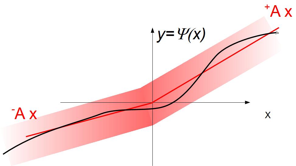
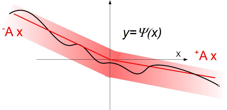
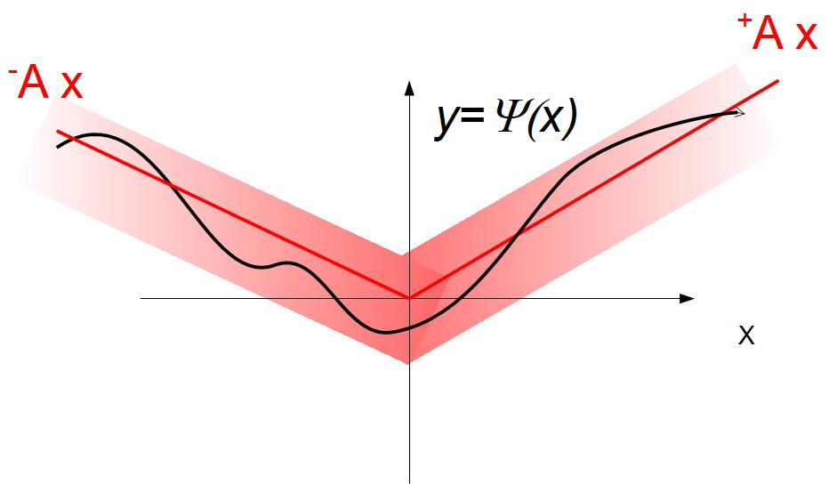
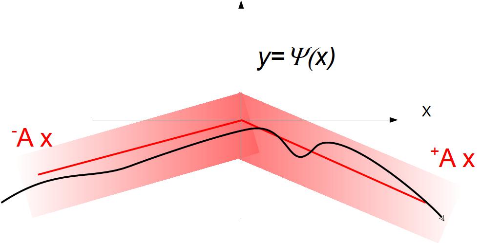
Figure 1: The four possible shapes of $\Psi$.
Slash-type $//$ (top left): ${}^{\scriptstyle-}\!A>0$ and ${}^{\scriptstyle+}\!A>0$, thus $-\Psi(-\infty)=\Psi(+\infty)=+\infty$.
Backslash-type \ (top right): ${}^{\scriptstyle-}\!A<0$ and ${}^{\scriptstyle+}\!A<0$, thus $\Psi(-\infty)=-\Psi(+\infty)=+\infty$.
Vee-type $\bigvee$ (bottom left): ${}^{\scriptstyle-}\!A<0<{}^{\scriptstyle+}\!A$, thus $\Psi(-\infty)=\Psi(+\infty)=+\infty$.
Wedge-type $\bigwedge$ (bottom right): ${}^{\scriptstyle+}\!A<0<{}^{\scriptstyle-}\!A$, thus $\Psi(-\infty)=\Psi(+\infty)=-\infty$.

Provided that the observed values of ${}^{{\scalebox{0.62}{ $\bm{-}$}}}A,{}^{{\scalebox{0.62}{ $\bm{+}$}}}A$ are both nonzero, the pertinent realization of $\Psi$ as a function may, regarding its overall shape, exhibit one of four distinct types as illustrated in Fig. 1. These are denoted mnemonically as slash-type $/$, backslash-type $\setminus$, vee-type $\vee$, and wedge-type $\wedge$. In the simple affine model with ${}^{{\scalebox{0.62}{ $\bm{+}$}}}A={}^{{\scalebox{0.62}{ $\bm{-}$}}}A=A>0$, the function $\Psi$ is always of slash-type. Goldie’s implicit renewal theory Goldie:91 is designed for ALIFS with $\Psi$ satisfying

$$|\Psi(x)-Ax|\ \leq\ B$$

for some random variables $A,B$. It therefore mixes functions of slash-type and backslash-type such that ${}^{{\scalebox{0.62}{ $\bm{-}$}}}A={}^{{\scalebox{0.62}{ $\bm{+}$}}}A$. The $\mathsf{AR}$(1)-model with $\mathsf{ARCH}$(1) errors provides an instance where functions of type $/$, $\bigvee$ and $\bigwedge$ are mixed. If the function $\Psi(x)$ is uniformly bounded for $x>0$ (resp. $x<0$), then ${}^{{\scalebox{0.62}{ $\bm{+}$}}}A=0$ (resp. ${}^{{\scalebox{0.62}{ $\bm{-}$}}}A=0$). This occurs, for instance, in the Beverton-Holt model.

In view of (4), it is natural to relate the ALIFS $X_{n}=\Psi_{n}\cdots\Psi_{1}(X_{0})$ with the $\mathsf{LIFS}$ $\Lambda_{n}\cdots\Lambda_{1}(X_{0})$ which in turn, following Kesten’s approach in the present one-dimensional setting, can be studied with the help of a suitable temporally homogeneous Markov chain $\Xi=(\xi_{n})_{n\geq 0}$. Namely, let $\xi_{0}:=\textsl{sign}(X_{0})$ and

$$\xi_{n}\,:=\,\textsl{sign}(\Lambda_{n}(\xi_{n-1}))\ =\ \begin{cases}\textsl{sign}({}^{{\scalebox{0.62}{ $\bm{-}$}}}A_{n})\xi_{n-1},&\text{if }\xi_{n-1}=-1,\\ \textsl{sign}({}^{{\scalebox{0.62}{ $\bm{+}$}}}A_{n})\xi_{n-1},&\text{if }\xi_{n-1}=1,\\ \hfill 0,&\text{if }\xi_{n-1}=0,\end{cases}$$ (6)

for $n\geq 1$. This chain has state space $\mathscr{S}=\mathbb{S}^{0}\cup\{0\}$, and the state 0, if it appears, is absorbing in which case at least one of the states $\pm 1$ must be transient. Whenever convenient, the set $\mathbb{S}^{0}$ is identified with the set of signs $\{-,+\}$ (e.g., in sub- or superscripts as in (5)) because $\xi_{n}$ keeps track of the sign of $\Lambda_{n}\cdots\Lambda_{1}(X_{0})$, that is $\xi_{n}=\textsl{sign}(\Lambda_{n}\cdots\Lambda_{1}(X_{0}))$ with $\Lambda_{n}\cdots\Lambda_{1}$ used as shorthand for $\Lambda_{n}\circ\cdots\circ\Lambda_{1}$. Let

$$p_{\delta\epsilon}\,:=\,\mathbb{P}[\xi_{n}=\epsilon|\xi_{n-1}=\delta]\ =\ \mathbb{P}[\textsl{sign}(^{\delta}A)\delta=\epsilon]$$

for $\delta,\epsilon\in\{-1,0,+1\}$, whence the possibly reduced and therefore substochastic transition matrix of $\Xi$ on $\mathbb{S}^{0}$ is given by

$$P\ =\ \begin{pmatrix}p_{\scriptscriptstyle--}&p_{\scriptscriptstyle-+}\\ p_{\scriptscriptstyle+-}&p_{\scriptscriptstyle++}\end{pmatrix}\ =\ \begin{pmatrix}\mathbb{P}[{}^{{\scalebox{0.62}{ $\bm{-}$}}}A>0]&\mathbb{P}[{}^{{\scalebox{0.62}{ $\bm{-}$}}}A<0]\\ \mathbb{P}[{}^{{\scalebox{0.62}{ $\bm{+}$}}}A<0]&\mathbb{P}[{}^{{\scalebox{0.62}{ $\bm{+}$}}}A>0]\end{pmatrix}.$$ (7)

As common, we put $\mathbb{P}_{\delta}:=\mathbb{P}[\cdot|\xi_{0}=\delta]$ and $\mathbb{P}_{\chi}:=\sum_{\delta\in\mathscr{S}}\chi_{\delta}\mathbb{P}_{\delta}$ for any measure $\chi$ on $\mathscr{S}$.

In order to state our main results on the tail behavior of any stationary distribution of the given ALIFS $(X_{n})_{n\geq 0}$, we distinguish three cases regarding the transition structure of the chain $\Xi$ (see Fig. 2).

Case 1 (irreducible case)

$p_{-+}>0$ and $p_{+-}>0$, that is both ${}^{{\scalebox{0.62}{ $\bm{+}$}}}A$ and ${}^{{\scalebox{0.62}{ $\bm{-}$}}}A$ are negative with positive probability. We will see that the tails of an invariant distribution $\nu$ at $+\infty$ and $-\infty$ are of the same order in this case.

Case 2 (unilateral case)

$p_{-+}>0$ and $p_{+-}=0$ , that is ${}^{{\scalebox{0.62}{ $\bm{-}$}}}A$ is negative with positive probability but ${}^{{\scalebox{0.62}{ $\bm{+}$}}}A\geq 0$. The functions $\Psi$ are only of types $/$ and $\vee$. In this case, the order of decay of $\nu$ at $+\infty$ can depend on both coefficients ${}^{{\scalebox{0.62}{ $\bm{+}$}}}A$ and ${}^{{\scalebox{0.62}{ $\bm{-}$}}}A$, while the behavior at $-\infty$ depends only on ${}^{{\scalebox{0.62}{ $\bm{-}$}}}A$. The corresponding case $p_{+-}>0$ and $p_{-+}=0$ can be treated without further ado after conjugation by $x\mapsto-x$.

Case 3 (separated case)

$p_{-+}=0$ and $p_{+-}=0$ , that is ${}^{{\scalebox{0.62}{ $\bm{-}$}}}A\geq 0$ and ${}^{{\scalebox{0.62}{ $\bm{+}$}}}A\geq 0$. The functions $\Psi$ are only of type $/$. In this case, the order of decay of the tail of $\nu$ at $+\infty$ (resp. $-\infty$) depends only on ${}^{{\scalebox{0.62}{ $\bm{+}$}}}A$ (resp. ${}^{{\scalebox{0.62}{ $\bm{-}$}}}A$).

Figure 2: The transition structure of $\Xi$ in the three cases 1–3. The dashed arrows indicate transitions that may have both positive or zero probability.

Fundamental tools in our study are the Cramér transform of $P$, defined by

$$P(\theta)\,:=\,\begin{pmatrix}p_{\scriptscriptstyle--}(\theta)&p_{\scriptscriptstyle-+}(\theta)\\ p_{\scriptscriptstyle+-}(\theta)&p_{\scriptscriptstyle++}(\theta)\end{pmatrix}\,:=\,\begin{pmatrix}\mathbb{E}|{}^{{\scalebox{0.62}{ $\bm{-}$}}}A|^{\theta}\mathbf{1}_{\{{}^{{\scalebox{0.62}{ $\bm{-}$}}}A>0\}}&\mathbb{E}|{}^{{\scalebox{0.62}{ $\bm{-}$}}}A|^{\theta}\mathbf{1}_{\{{}^{{\scalebox{0.62}{ $\bm{-}$}}}A<0\}}\\ \mathbb{E}|{}^{{\scalebox{0.62}{ $\bm{+}$}}}A|^{\theta}\mathbf{1}_{\{{}^{{\scalebox{0.62}{ $\bm{+}$}}}A<0\}}&\mathbb{E}|{}^{{\scalebox{0.62}{ $\bm{+}$}}}A|^{\theta}\mathbf{1}_{\{{}^{{\scalebox{0.62}{ $\bm{+}$}}}A>0\}}\end{pmatrix}$$ (8)

for $\theta\in\mathbb{D}:=\{\vartheta\geq 0:\mathbb{E}|{}^{{\scalebox{0.62}{ $\bm{-}$}}}A|^{\vartheta}+\mathbb{E}|{}^{{\scalebox{0.62}{ $\bm{+}$}}}A|^{\vartheta}<\infty\}$, and its dominant eigenvalue (spectral radius) $\rho(\theta)$. They will be discussed in greater detail in Subsection 4.1

Case 1 (irreducible case). $p_{-+}>0$ and $p_{+-}>0$.
In this case, the dominant eigenvalue $\rho(\theta)$ is associated to the left and right nonnegative eigenvectors

$$u(\theta)\,=\,(u_{\scriptscriptstyle-}(\theta),u_{\scriptscriptstyle+}(\theta))^{\top}\quad\text{and}\quad v(\theta)\,=\,(v_{\scriptscriptstyle-}(\theta),v_{\scriptscriptstyle+}(\theta))^{\top},$$

respectively, uniquely determined by $u(\theta)^{\top}v(\theta)=1$ and $u_{\scriptscriptstyle+}(\theta)+u_{\scriptscriptstyle-}(\theta)=1$. This implies that

$$\widehat{\pi}(\theta)\,:=\,\big{(}u_{\scriptscriptstyle-}(\theta)v_{\scriptscriptstyle-}(\theta),u_{\scriptscriptstyle+}(\theta)v_{\scriptscriptstyle+}(\theta)\big{)}^{\top}.$$ (9)

forms a probability distribution. For $\theta>0$, it will later be identified as the stationary law of $(\xi_{n})_{n\geq 0}$ after a suitable change of measure. For $\theta=0$, this is only true when $P$ is stochastic or, equivalently,

$$\mathbb{P}[{}^{{\scalebox{0.62}{ $\bm{-}$}}}A=0]\ =\ \mathbb{P}[{}^{{\scalebox{0.62}{ $\bm{+}$}}}A=0]\ =\ 0$$ (10)

holds in which case

$$\pi\ =\ \left(\frac{p_{\scriptscriptstyle+-}}{p_{\scriptscriptstyle-+}+p_{\scriptscriptstyle+-}},\frac{p_{\scriptscriptstyle-+}}{p_{\scriptscriptstyle-+}+p_{\scriptscriptstyle+-}}\right)^{\top}\ =\ \widehat{\pi}(0)$$ (11)

equals the unique associated stationary distribution of $\Xi$.

The crucial assumption in the subsequent theorem is that

$$\rho(\kappa)\,=\,1\quad\text{for some }\kappa>0.$$ (12)

We denote by $\mathscr{C}^{*}(\mathbb{R})$ the space of bounded Lipschitz functions $\phi$ on $\mathbb{R}$ which vanish in a neighborhood of the origin and by $\mathscr{C}_{-}^{*}(\mathbb{R}),\,\mathscr{C}_{+}^{*}(\mathbb{R})$ the subspaces of those $\phi$ that also vanish on $\mathbb{R}_{\scriptscriptstyle\geqslant},\,\mathbb{R}_{\scriptscriptstyle\leqslant}$, respectively.

Theorem 2.1

Assuming (12),

$$\mathbb{E}|{}^{\delta}\!A|^{\kappa}\log|{}^{\delta}\!A|\,<\,\infty\text{ for $\delta\in\{-,+\}$,}\quad\mathbb{E}B^{\kappa}\,<\,\infty$$ (13)

and

$$\mathbb{P}_{\widehat{\pi}(\kappa)}[\log|{}^{\xi_{0}}\!A|-a_{\xi_{1}}+a_{\xi_{0}}\in d\mathbb{Z}]\,<\,1\quad\text{for all }d>0\text{ and }a_{\pm}\in\mathbb{R},$$ (14)

any stationary distribution $\nu$ of the ALIFS $(X_{n})_{n\geq 0}$ has power tails of order $\kappa$, more precisely

$$\lim_{t\to\infty}t^{\kappa}\,\nu((t,\infty))\,=\,C_{\scriptscriptstyle+}\quad\text{and}\quad\lim_{t\to\infty}t^{\kappa}\,\nu((-\infty,-t))\,=\,C_{\scriptscriptstyle-}$$ (15)

for constants $C_{\scriptscriptstyle+},C_{\scriptscriptstyle-}\geq 0$ which are explicitly defined in (78),(79) and satisfy

$$u_{\scriptscriptstyle+}(\kappa)\,C_{\scriptscriptstyle-}\ =\ u_{\scriptscriptstyle-}(\kappa)\,C_{\scriptscriptstyle+}.$$ (16)

Furthermore,

$$\lim_{t\to\infty}t^{\kappa}\int\phi(t^{-1}x)\ \nu(dx)\ =\ \kappa\int_{0}^{\infty}\frac{C_{\scriptscriptstyle-}\phi(-x)+C_{\scriptscriptstyle+}\phi(x)}{x^{\kappa+1}}\ dx$$ (17)

for any $\phi\in\mathscr{C}^{*}(\mathbb{R})$.

Further information on the lattice-type Condition (14) will be provided later, see Subsect. 4.3.

Observe that the above result concerns the asymptotic behavior of the tail of the stationary measure. Our proof, which is based on a renewal theorem, does not entail the positivity of the limiting constants $C_{\scriptscriptstyle+},C_{\scriptscriptstyle-}$. However, we will be able to verify this in Section 8 under the additional assumption that the stationary measure has unbounded support (see Proposition 8.1).

Case 2 (unilateral case). $p_{-+}>0$ and $p_{+-}=0$.
In this case, the crucial numbers, if they exist, are $\kappa_{\scriptscriptstyle-},\kappa_{\scriptscriptstyle+}>0$ defined by

$$p_{\scriptscriptstyle--}(\kappa_{-})\,=\,1\quad\text{and}\quad p_{\scriptscriptstyle++}(\kappa_{\scriptscriptstyle+})\,=\,1.$$

As a substitute for Condition (13), we need that either

$$\mathbb{E}|{}^{{\scalebox{0.62}{ $\bm{-}$}}}A|^{\kappa}\log|{}^{{\scalebox{0.62}{ $\bm{-}$}}}A|\,<\,\infty\quad\text{and}\quad\mathbb{E}B^{\kappa}\,<\,\infty$$ (18)

or

$$\mathbb{E}|{}^{{\scalebox{0.62}{ $\bm{+}$}}}A|^{\kappa}\log|{}^{{\scalebox{0.62}{ $\bm{+}$}}}A|\,<\,\infty\quad\text{and}\quad\mathbb{E}B^{\kappa}\,<\,\infty.$$ (19)

Theorem 2.2

(a) If $\kappa_{\scriptscriptstyle-}$ exists, Condition (18) holds for $\kappa=\kappa_{\scriptscriptstyle-}$ and $\mathbb{P}[\log|{}^{{\scalebox{0.62}{ $\bm{-}$}}}A|\in\cdot|{}^{{\scalebox{0.62}{ $\bm{-}$}}}A>0]$ is nonarithmetic, then any stationary distribution $\nu$ satisfies

$$\lim_{t\to\infty}t^{\kappa_{\scriptscriptstyle-}}\,\nu((-\infty,-t))\,=\,C_{\scriptscriptstyle-}$$ (20)

as well as

$$\lim_{t\to\infty}t^{\kappa_{\scriptscriptstyle-}}\int\phi(t^{-1}x)\ \nu(dx)\ =\ \kappa_{\scriptscriptstyle-}\int_{0}^{\infty}\frac{C_{\scriptscriptstyle-}\phi(-x)}{x^{\kappa_{\scriptscriptstyle-}+1}}\ dx$$ (21)

for $\phi\in\mathscr{C}_{-}^{*}(\mathbb{R})$, where $C_{\scriptscriptstyle-}$ is defined in (85).

(b) If $\kappa_{\scriptscriptstyle+}$ exists, $p_{\scriptscriptstyle--}(\kappa_{\scriptscriptstyle+})<1$ (thus $\kappa_{\scriptscriptstyle-}$, if it exists, is greater than $\kappa_{\scriptscriptstyle+}$), $p_{\scriptscriptstyle-+}(\kappa_{\scriptscriptstyle+})<\infty$, Condition (19) holds for $\kappa=\kappa_{\scriptscriptstyle+}$ and $\mathbb{P}[\log|{}^{{\scalebox{0.62}{ $\bm{+}$}}}A|\in\cdot|{}^{{\scalebox{0.62}{ $\bm{+}$}}}A>0]$ is nonarithmetic, then any stationary distribution $\nu$ satisfies

$$\lim_{t\to\infty}t^{\kappa_{\scriptscriptstyle+}}\,\nu((t,\infty))\,=\,C_{\scriptscriptstyle+}$$ (22)

as well as

$$\lim_{t\to\infty}t^{\kappa_{\scriptscriptstyle+}}\int\phi(t^{-1}x)\ \nu(dx)\ =\ \kappa_{\scriptscriptstyle+}\int_{0}^{\infty}\frac{C_{\scriptscriptstyle+}\phi(x)}{x^{\kappa_{\scriptscriptstyle+}+1}}\ dx$$ (23)

for $\phi\in\mathscr{C}^{*}(\mathbb{R})$, where $C_{\scriptscriptstyle+}$ is defined in (84).

(c) If $\kappa_{\scriptscriptstyle-}$ exists, $p_{\scriptscriptstyle++}(\kappa_{\scriptscriptstyle-})<1$ (thus $\kappa_{\scriptscriptstyle-}<\kappa_{\scriptscriptstyle+}$ if the latter exists as well), $p_{\scriptscriptstyle++}(\theta)<1$ and $p_{\scriptscriptstyle-+}(\theta)<\infty$ for some $\theta>\kappa_{\scriptscriptstyle-}$, Condition (18) holds for $\kappa=\kappa_{\scriptscriptstyle-}$ and $\mathbb{P}_{\scriptscriptstyle-}[\log|{}^{{\scalebox{0.62}{ $\bm{-}$}}}A|\in\cdot|{}^{{\scalebox{0.62}{ $\bm{-}$}}}A>0]$ is nonarithmetic, then any stationary distribution $\nu$ satisfies

$$\lim_{t\to\infty}t^{\kappa_{\scriptscriptstyle-}}\,\nu((t,\infty))\ =\ C_{\scriptscriptstyle-}^{\scriptscriptstyle+}$$ (24)

as well as

$$\lim_{t\to\infty}t^{\kappa_{\scriptscriptstyle-}}\int\phi(t^{-1}x)\ \nu(dx)\ =\ \kappa_{\scriptscriptstyle-}\int_{0}^{\infty}\frac{C_{\scriptscriptstyle-}\phi(-x)+C_{\scriptscriptstyle-}^{\scriptscriptstyle+}\phi(x)}{x^{\kappa_{\scriptscriptstyle-}+1}}\ dx$$ (25)

for $\phi\in\mathscr{C}^{*}(\mathbb{R})$, where $C_{\scriptscriptstyle-},\,C_{\scriptscriptstyle-}^{\scriptscriptstyle+}$ are defined in (85) and (86), respectively.

Observe that if both $\kappa_{\scriptscriptstyle-}$ and $\kappa_{\scriptscriptstyle+}$ exist with $\kappa_{\scriptscriptstyle-}>\kappa_{\scriptscriptstyle+}$, then cases (a) and (b) entail that the stationary measure behaves regularly at $+\infty$ and $-\infty$, but with different tail decay rates.

The unilateral case shares several features with the study of the stationary distribution of the two-dimensional recursive Markov chain defined by the affine recursions $\Psi_{n}(x)=A_{n}x+B_{n}$ in the case when the $A_{n}$ are upper triangular matrices. Such models have attracted some interest in recent years due to their relevance for some models in econometrics, see DMS19 .

Regarding the case $\kappa_{+}=\kappa_{-}$, we further remark that the methods used in the present paper are not strong enough and thus need to be refined. It seems reasonable to believe that in this case a first order expansion of $P(\theta)$ in $\kappa$ is required with a possible extra term in the power tail of $\nu$, see again DZ18 for similar considerations in the case of the afore-mentioned two-dimensional recursions.

Case 3 (separated case). $p_{\scriptscriptstyle-+}=0$ and $p_{\scriptscriptstyle+-}=0$.
This is the easiest case and can be treated by Goldie’s implicit renewal theory Goldie:91 . We state the result here for completeness and put

$$C_{\delta}\,:=\,\frac{\mathbb{E}\big{[}|\Psi(R)|^{\kappa_{\delta}}\mathbf{1}_{\{\Psi(R)<0\}}-|^{\delta}AR|^{\kappa_{\delta}}\mathbf{1}_{\{\delta R>0\}}\big{]}}{\kappa_{\delta}\,p_{\delta\delta}^{\prime}(\kappa_{\delta})}$$

for $\delta\in\{-,+\}$.

Theorem 2.3

(a) If $\kappa_{\scriptscriptstyle-}$ exists, Condition (18) holds for $\kappa=\kappa_{\scriptscriptstyle-}$ and $\log|{}^{{\scalebox{0.62}{ $\bm{-}$}}}A|$ is nonarithmetic, then any stationary distribution $\nu$ satisfies

$$\lim_{t\to\infty}t^{\kappa_{\scriptscriptstyle-}}\,\nu((-\infty,-t))\,=\,C_{\scriptscriptstyle-}$$ (26)

where $R$ has law $\nu$ and is independent of $\Psi,{}^{{\scalebox{0.62}{ $\bm{-}$}}}A$. Moreover, (21) holds for any $\phi\in\mathscr{C}_{-}^{*}(\mathbb{R})$ and with $C_{\scriptscriptstyle-}$ as in (26).

(b) If $\kappa_{\scriptscriptstyle+}$ exists, Condition (19) holds for $\kappa=\kappa_{\scriptscriptstyle+}$ and $\log|{}^{{\scalebox{0.62}{ $\bm{+}$}}}A|$ is nonarithmetic, then any stationary distribution $\nu$ on $\mathbb{R}_{\scriptscriptstyle>}$ satisfies

$$\lim_{t\to\infty}t^{\kappa_{\scriptscriptstyle+}}\,\nu((t,\infty))\,=\,C_{\scriptscriptstyle+}$$ (27)

here $R$ has law $\nu$ and is independent of $\Psi,{}^{{\scalebox{0.62}{ $\bm{+}$}}}A$. Moreover, (23) holds for any $\phi\in\mathscr{C}_{+}^{*}(\mathbb{R})$ and with $C_{\scriptscriptstyle+}$ as in (27).

In any of the three cases the conditions (12) and (13) ensure the existence of at least one stationary distribution of $(X_{n})_{n\geq 0}$. We refer to Section 9 for details.

2.1 Examples

Let us briefly discuss some examples of ALIFS that have appeared in the literature and whose stationary distributions exhibit a tail behavior that, under appropriate conditions, can be read off from our main results. In order to keep this presentation short, we refrain from giving any technical details. Further applications with a more thorough discussion can be found in BroBura:13 .

$\mathsf{ARCH}$(1)

Our first example, the autoregressive conditional heteroskedasticity model of order one, is well-known in econometrics and usually defined by the pair of recursive equations

$$X_{n}\,=\,\Sigma_{n}Z_{n}\quad\text{and}\quad\Sigma_{n}^{2}\,=\,\beta+\lambda X^{2}_{n-1},$$

where $(Z_{n})_{n\geq 1}$ denotes a sequence of i.i.d. random variables with mean zero and variance one (the noise) and $\beta,\lambda$ are positive parameters. Simple inspection shows that this entails the recursive relation $X_{n}=\Psi_{n}(X_{n-1})$ for $n\geq 1$ and i.i.d. copies $\Psi_{1},\Psi_{2},\ldots$ of the random function

$$\Psi(x)\,=\,Z\sqrt{\beta+\lambda x^{2}}.$$

As one can also readily check, $(X_{n})_{n\geq 0}$ forms an ALIFS which satisfies (4) with ${}^{\scriptscriptstyle\pm}A_{n}=\pm Z_{n}\sqrt{\lambda_{n}}$ and is irreducible (Case 1). Unless $Z$ has a symmetric law, the constants $C_{+},C_{-}$ defined in (15) are generally distinct. Let us also point out here that $(X_{n})_{n\geq 0}$ remains an ALIFS if the parameters $\beta_{n}$ and $\lambda_{n}$ are allowed to be random.

$\mathsf{AR}$(1) models with $\mathsf{ARCH}$(1) errors

This extension of the previous example is obtained by adding an extra linear term and therefore defined as the ALIFS generated by i.i.d. copies of the random function

$$\Psi(x)\,=\,\alpha x+Z\left(\beta+\lambda x^{2}\right)^{1/2}$$

for some $(\alpha,\beta,\lambda)\in\mathbb{R}\times\mathbb{R}_{\scriptscriptstyle>}^{2}$ and a random variable $Z$ as before. It satisfies (4) with ${}^{\scriptscriptstyle\pm}A=\alpha\pm Z\sqrt{\lambda}$. Depending on the parameters $\alpha,\lambda$ and the almost sure range of $Z$, all three cases introduced above may occur. We will return to this example in Section 10 at the end of this work.

$\mathsf{IFS}$ on the unit interval

Consider an $\mathsf{IFS}$ generated by i.i.d. copies of a random continuous self-map $\Phi$ of the unit interval $[0,1]$ which further satisfies $\Phi((0,1))\subseteq(0,1)$. If $\Phi$ is twice differentiable at $0$ and $1$, this $\mathsf{IFS}$ can be conjugated to obtain an ALIFS of the real line. Namely, by taking the diffeomorphism $r$ of $(0,1)$ onto $\mathbb{R}$, defined by

$$r(u)\,:=\,-\frac{1}{u}+\frac{1}{1-u},$$

the conjugated function $\Psi=r\circ\Phi\circ r^{-1}$ satisfies (4) with

$${}^{{\scalebox{0.62}{ $\bm{-}$}}}A\,=\,\begin{cases}\frac{1}{\Phi^{\prime}(0)}&\text{if }\Phi(0)=0\text{ or }1\\ \hfill 0&\text{if }\Phi(0)\in(0,1)\end{cases}\quad\text{and}\quad{}^{{\scalebox{0.62}{ $\bm{+}$}}}A\,=\,\begin{cases}\frac{1}{\Phi^{\prime}(1)}&\text{if }\Phi(1)=0\text{ or }1\\ \hfill 0&\text{if }\Phi(1)\in(0,1)\end{cases},$$

(see Section 6.3 in BroBura:13 for more details). Note further that $\nu$ is an invariant distribution for the $\mathsf{IFS}$ generated by $\Phi$ (i.e. $\Phi(X)\stackrel{{\scriptstyle d}}{{=}}\nu$ if $X\stackrel{{\scriptstyle d}}{{=}}\nu$, where $\stackrel{{\scriptstyle d}}{{=}}$ means equality in law) iff $r*\nu$ is invariant for the ALIFS generated by $\Psi$. Thus, under appropriate hypotheses, this system possesses a stationary distribution whose behaviour close to the boundaries of the interval can be deduced from our main results. As a particular instance which has received some attention in the literature, we mention here the random logistic transform $\Phi(x)=Ax(1-x)$ with $0<A<4$ a.s., ${}^{{\scalebox{0.62}{ $\bm{-}$}}}A=1/\alpha$ and ${}^{{\scalebox{0.62}{ $\bm{+}$}}}A=1/\alpha$, see e.g. AthreyaDai:00 .

2.2 Structure of the paper

The principal goal of this work is to describe the tail behavior of a stationary measure $\nu$ of an ALIFS at $\pm\infty$. In Sections 3 and 4, we provide the indispensable tools to prove our main results. Then we prove the existence of the limits in Theorems 2.1, 2.2 and 2.3 in Sections 5, 6 and 7, respectively. It will be seen that the nondegeneracy of the limits, i.e., the positivity of the limiting constants requires different arguments and in fact forms a separate problem. This question is postponed until Section 8 and there taken care of in Proposition 8.1. In Section 9, we give conditions for the existence of at least one stationary distribution $\nu$ (see Prop. 9.1) which are directly seen to be valid in our main theorems. Uniqueness of $\nu$ will not be discussed here, because this requires geometric arguments and a local analysis of the process which in such generality is beyond the scope of this work. The AR(1) model with GARCH errors is an example which has received some interest in the literature Alsmeyer:16 ; BorkovecKl:01 ; GueDie:94 ; Maercker:97 and to which our results can be applied, in fact with all three cases being possible. It will therefore be discussed in greater detail in the final Section 10, followed by a short appendix containing a technical lemma about the maximal eigenvalue $\rho(\theta)$ in a right neighborhood of 0.

3 Prerequisites

3.1 The induced Markov random walk

Defining ${S_{0}}:=\log|X_{0}|$ and

$$S_{n}\,:=\,\log|\Lambda_{n}\cdots\Lambda_{1}(X_{0})|$$

for $n\geq 1$ (with the usual convention $\log 0:=-\infty$), we see that, given $\Xi$, the increments $\zeta_{n}:=S_{n}-S_{n-1}=\log|\Lambda_{n}(\xi_{n-1})|$, $n=1,2,,\ldots$, are conditionally independent and

$$\mathbb{P}[\zeta_{n}\in\cdot|\Xi,\xi_{n-1}=\delta,\xi_{n}=\epsilon]\ =\ \mathbb{P}[\log|\Lambda_{n}(\xi_{n-1})|\in\cdot|\xi_{n-1}=\delta,\xi_{n}=\epsilon]$$

$$=\ \mathbb{P}[\log|^{\delta}A|\in\cdot|\delta\cdot\textsl{sign}(^{\delta}A)=\epsilon].$$

Equivalently, $(\xi_{n},\zeta_{n})_{n\geq 0}$ forms a Markov chain such that the conditional law of $(\xi_{n},\zeta_{n})$ given the past depends on $\xi_{n-1}$ only. The transition kernel equals

$$Q(\delta,\{\epsilon\}\times B)\ =\ \mathbb{P}[\delta\cdot\textsl{sign}(^{\delta}A)=\epsilon,\,\log|^{\delta}A|\in B]$$

for measurable $B\subset\mathbb{R}$, $\delta\in\mathbb{S}^{0}$ and $\epsilon\in\mathscr{S}$. If $\delta=0$, then $Q(\delta,\cdot)$ equals Dirac measure at $\dagger:=(0,-\infty)$. In other words, $\dagger$ is an absorbing state for $(\xi_{n},\zeta_{n})_{n\geq 0}$ and should be viewed as a grave. It follows that $(\xi_{n},S_{n})_{n\geq 0}$ does indeed constitute a Markov random walk ($\mathsf{MRW}$) with discrete driving chain $\Xi$ and induced by $(\Lambda_{n}\cdots\Lambda_{1}(X_{0}))_{n\geq 1}$. However, it may be absorbed at $\dagger$ in finite time (explosion of the additive part). On the other hand, the conditions in our main Theorems 2.1–2.3 ensure that, after a suitable change of measure $\mathbb{P}\rightsquigarrow\widehat{\mathbb{P}}$ to be decribed in Subsection 4.2, the driving chain has state space $\mathbb{S}^{0}$ and explosion does no longer occur. The relevant renewal-theoretic properties of the $\mathsf{MRW}$ after this measure change, which is essential for the analysis of the tails of the stationary distributions of $(X_{n})_{n\geq 0}$, will be discussed in Subsection 4.3.

3.2 Standard model

It is convenient to assume a standard model

$$(\Omega,\mathfrak{A},(\mathbb{P}_{x})_{x\in\mathbb{R}},(\xi_{n},S_{n})_{n\geq 0}),$$

where $(\Omega,\mathfrak{A})$ denotes the measurable space on which all occurring random variables are defined and $\mathbb{P}_{x}:=\mathbb{P}[\cdot|X_{0}=x]$, thus

$$\mathbb{P}_{x}[X_{0}=x,\xi_{0}=\textsl{sign}(x),S_{0}=\log|x|]\ =\ 1$$

for all $x\in\mathbb{R}$. The definition extends the one given before in Thm. 2.1 in a compatible way because $\mathbb{P}_{\delta}[\xi_{0}=\delta]=1$ if $\delta\in\mathscr{S}$. Moreover, we put $\mathbb{P}_{\chi}:=\int\mathbb{P}_{x}\,\chi(dx)$ for any measure $\chi$ on $\mathbb{R}$ and use $\mathbb{P}$ for probabilities that do not depend on initial conditions.

3.3 Associated $\mathsf{LIFS}$

The fact that $\Psi_{1},\Psi_{2},\ldots$ are i.i.d. implies that, for each $n\in\mathbb{N}_{0}$, the forward iteration $X_{n}$ and the backward iteration $\widehat{X}_{n}:=\Psi_{1}\cdots\Psi_{n}(X_{0})$ have the same distribution, more precisely

$$X_{n}\ =\ \Psi_{n}\cdots\Psi_{1}(X_{0})\ \stackrel{{\scriptstyle d}}{{=}}\ \Psi_{1}\cdots\Psi_{n}(X_{0})\ =\ \widehat{X}_{n}\quad\text{under }\mathbb{P}_{x}$$ (28)

for each $n\in\mathbb{N}_{0}$. By a similar argument and in analogy with (28),

$$\Lambda_{n}\cdots\Lambda_{1}(x)\ \stackrel{{\scriptstyle d}}{{=}}\ \Lambda_{1}\cdots\Lambda_{n}(x)\quad\text{under }\mathbb{P}_{x}$$

for all $n\in\mathbb{N}$ and $x\in\mathbb{R}$.

The following simple but crucial lemma is a consequence of Condition (4). Given a Lipschitz continuous function $f$, let $\textsf{Lip}\hskip 1.0pt(f)$ be its Lipschitz constant. Note that $\textsf{Lip}\hskip 1.0pt(\Lambda)=|{}^{{\scalebox{0.62}{ $\bm{-}$}}}A|\vee|{}^{{\scalebox{0.62}{ $\bm{+}$}}}A|$. Further putting $\Phi_{n}(x):=\textsf{Lip}\hskip 1.0pt(\Lambda_{n})x+B_{n}$ for $n\in\mathbb{N}$, we introduce the $\mathsf{LIFS}$  $(Z_{n})_{n\geq 0}$ and the associated ”error term” $(Y_{n})_{n\geq 0}$ by setting $Y_{0}:=0$, $Z_{0}:=X_{0}$,

$$Z_{n}\,:=\,\Lambda_{n}\cdots\Lambda_{1}(Z_{0})\quad\text{and}\quad Y_{n}\,:=\,\sum_{k=1}^{n}\textsf{Lip}\hskip 1.0pt(\Lambda_{n}\ldots\Lambda_{k+1})B_{k}$$

for $n\geq 1$. The corresponding backward iterations are

$$\widehat{Z}_{n}\,:=\,\Lambda_{1}\cdots\Lambda_{n}(Z_{0})\quad\text{and}\quad\widehat{Y}_{n}\,:=\,\sum_{k=1}^{n}L^{\to}_{k-1}B_{k},$$ (29)

where $L^{\to}_{k}\,:=\,\textsf{Lip}\hskip 1.0pt(\Lambda_{1}\cdots\Lambda_{k})$ for $k\in\mathbb{N}$ and $L^{\to}_{0}:=1$.

Lemma 3.1

If Condition (4) holds true, then

$$\sup_{x\in\mathbb{R}}|\Psi_{n}\cdots\Psi_{1}(x)-\Lambda_{n}\cdots\Lambda_{1}(x)|\ \leq\ Y_{n},$$ (30)

$$\sup_{x\in\mathbb{R}}|\Psi_{1}\cdots\Psi_{n}(x)-\Lambda_{1}\cdots\Lambda_{n}(x)|\ \leq\ \widehat{Y}_{n},$$ (31)

and in particular

$$|X_{n}-Z_{n}|\ \leq\ Y_{n}\quad\text{and}\quad|\widehat{X}_{n}-\widehat{Z}_{n}|\ \leq\ \widehat{Y}_{n}$$ (32)

for all $n\in\mathbb{N}$.

Proof

It suffices to prove (31) for which we use induction over $n$. Note that (4) provides the assertion for $n=1$. Assuming the assertion be true for $n-1$ (inductive hypothesis), we infer for any $x\in\mathbb{R}$

$$|\Psi_{1}\cdots\Psi_{n}(x)-\Lambda_{1}\cdots\Lambda_{n}(x)|$$

$$\hskip 28.45274pt\leq\ |\Psi_{1}\cdots\Psi_{n}(x)-\Lambda_{1}\cdots\Lambda_{n-1}(\Psi_{n}(x))|$$

$$\hskip 34.14322pt+\ |\Lambda_{1}\cdots\Lambda_{n-1}(\Psi_{n}(x))-\Lambda_{1}\cdots\Lambda_{n-1}(\Lambda_{n}(x))|$$

$$\hskip 28.45274pt\leq\ \widehat{Y}_{n-1}\,+\,L^{\to}_{n-1}|\Psi_{n}(x)-\Lambda_{n}(x)|$$ (33)

$$\hskip 28.45274pt\leq\ \widehat{Y}_{n-1}\,+\,L^{\to}_{n-1}B_{n}.$$

Since, by (29), the last line equals $\widehat{Y}_{n}$, the proof is complete. ∎

4 Transfer operators

Aiming at the tail behavior of the stationary distributions of the given ALIFS $(X_{n})_{n\geq 0}$ at $\pm\infty$, the Markov chain $(\xi_{n})_{n\geq 0}$ on the set $\mathbb{S}^{0}$ and its possibly reduced transition matrix $P$ will play an important role. Similar to the work by Goldie Goldie:91 and Kesten Kesten:73 , our approach uses a linear approximation, here of $X_{n}$ by the $\mathsf{LIFS}$ $Z_{n}=\Lambda_{n}\cdots\Lambda_{1}(Z_{0})$, see Lemma 3.1, and renewal-theoretic arguments after a suitable change of measure. The latter means to find a harmonic transform under which $\mathbb{S}^{0}$ becomes the proper state space of $(\xi_{n})_{n\geq 0}$, thus making absorption at 0 impossible if this state appears at all. For the case when $\log|Z_{n}|=S_{n}$ has i.i.d. increments and thus forms an ordinary random walk on $\mathbb{R}$, this transform is usually obtained with the help of moment generating functions. The method has indeed been effectively employed in Goldie:91 and Mirek:11 in the study of asymptotically linear stochastic equations, see also BurDamMik:16 . In the present context, however, the sequence $(S_{n})_{n\geq 0}$ has increments whose distributions are modulated by a two-state Markov chain, and if this chain is irreducible, then $(\xi_{n},S_{n})_{n\geq 0}$ constitutes a genuine $\mathsf{MRW}$ instead of an ordinary one. This in turn calls for the more advanced tool of so-called transfer operators, as in Kesten:73 ; AlsMen:12 ; BurDamGuiMen:14 ; GuivarchLePage:16 for the analysis of multidimensional problems and with a $\mathsf{MRW}$ whose driving chain has state space $\mathbb{S}^{d-1}$, the $d$-dimensional unit sphere in $\mathbb{R}^{d}$ for some $d\geq 2$. Since $\mathbb{S}^{0}$ has only two elements, the transfer operators reduce here to fairly simple objects, namely $2\times 2$ matrices.

4.1 The Cramér transform of $P$

Recall from (8) the definition of the Cramér transform $P(\theta)$ of the transition matrix $P$ on its canonical domain $\mathbb{D}=\{\theta\geq 0:\mathbb{E}|{}^{{\scalebox{0.62}{ $\bm{-}$}}}A|^{\theta}+\mathbb{E}|{}^{{\scalebox{0.62}{ $\bm{+}$}}}A|^{\theta}<\infty\}$, in particular $P(0)=P$ and

$$p_{\delta\epsilon}(\theta)\ =\ \mathbb{E}|^{\delta}A|^{\theta}\mathbf{1}_{\{\textsl{sign}(^{\delta}A)=\delta\epsilon\}}\ =\ \mathbb{E}_{\delta}\Big{[}e^{\theta S_{1}}\mathbf{1}_{\{\xi_{1}=\epsilon\}}\Big{]},$$ (34)

the latter being a log-convex function on $\mathbb{D}$. We make the further assumption that

$$\theta_{\infty}\,:=\,\sup\mathbb{D}\ >\ 0.$$ (35)

Let $\rho(\theta)$ be the dominant eigenvalue of $P(\theta)$ for $\theta\in\mathbb{D}$, explicitly given by

$$\small\rho(\theta)\ =\ \frac{p_{\scriptscriptstyle--}(\theta)+p_{\scriptscriptstyle++}(\theta)}{2}+\sqrt{\frac{(p_{\scriptscriptstyle--}(\theta)-p_{\scriptscriptstyle++}(\theta))^{2}}{4}+p_{\scriptscriptstyle-+}(\theta)p_{\scriptscriptstyle+-}(\theta)}\ >\ 0.$$ (36)

The matrix $P(\theta)$ and its spectral radius are strongly related to the product $\Lambda_{n}\cdots\Lambda_{1}$ as confirmed by the subsequent lemma. Let $p_{\delta\epsilon}^{n}(\theta)=[P(\theta)^{n}]_{\delta,\epsilon}$ denote the entries of $P(\theta)^{n}$. We note that the $n$-step transition probability $p_{\delta\epsilon}^{n}(\theta)$ should not be confused with $p_{\delta\epsilon}(\theta)^{n}$, the $n^{th}$ power of $p_{\delta\epsilon}(\theta)$, which does also appear later.

Lemma 4.1

For any $\theta\in\mathbb{D}$ and $\epsilon,\delta\in\mathbb{S}^{0}$

$$p_{\delta\epsilon}^{n}(\theta)\,=\,\mathbb{E}|\Lambda_{n}\cdots\Lambda_{1}(\delta)|^{\theta}\mathbf{1}_{\{\textsl{sign}(\Lambda_{n}\cdots\Lambda_{1}(\delta))=\epsilon\}}$$ (37)

and

$$\lim_{n\to\infty}\frac{1}{n}\log\mathbb{E}\,\textsf{Lip}\hskip 1.0pt(\Lambda_{n}\cdots\Lambda_{1})^{\theta}\,=\,\log\rho(\theta).$$ (38)

Proof

The relation (37) can be proved by induction over $n$. For $n=1$, it holds true by (34), and for the inductive step we note that

$$p_{\delta\epsilon}^{n+1}(\theta)\, =\,\sum_{s\in\mathbb{S}^{0}}p_{\delta s}(\theta)p_{s\epsilon}^{n}(\theta)$$

$$=\,\sum_{s\in\mathbb{S}^{0}}\mathbb{E}|\Lambda_{1}(\delta)|^{\theta}\mathbf{1}_{\{\textsl{sign}(\Lambda_{1}(\delta))=s\}}|\Lambda_{n+1}\cdots\Lambda_{2}(s)|^{\theta}\mathbf{1}_{\{\textsl{sign}(\Lambda_{n+1}\cdots\Lambda_{2}(s))=\epsilon\}}$$

$$=\,\mathbb{E}|\Lambda_{n+1}\cdots\Lambda_{1}(\delta)|^{\theta}\mathbf{1}_{\{\textsl{sign}(\Lambda_{n+1}\cdots\Lambda_{1}(\delta))=\epsilon\}}.$$

In particular, the norm of $P^{n}(\theta)$ as an operator on $(\mathbb{R}^{2},|\cdot|_{\infty})$ equals

$$\|P^{n}(\theta)\|_{\infty}\ =\ \max_{\delta}\left(p_{\delta+}^{n}(\theta)+p_{\delta-}^{n}(\theta)\right)\ =\ \max_{\delta}\mathbb{E}\left[|\Lambda_{n}\cdots\Lambda_{1}(\delta)|^{\theta}\right].$$

Hence

$$\|P^{n}(\theta)\|_{\infty}\ \leq\ \mathbb{E}\,\textsf{Lip}\hskip 1.0pt(\Lambda_{n}\cdots\Lambda_{1})^{\theta}\ \leq\ 2\|P^{n}(\theta)\|_{\infty}$$

and Gelfand’s formula yields (38). ∎

For further discussion, we consider the three cases as introduced in Section 2 separately.

Case 1. $p_{\scriptscriptstyle-+}\wedge p_{\scriptscriptstyle+-}>0$, i.e. $P$ is irreducible.
Then there are uniquely determined left and right nonnegative eigenvectors $u(\theta),v(\theta)$, respectively, satisfying

$$u(\theta)^{\top}v(\theta)\,=\,1\quad\text{and}\quad u_{\scriptscriptstyle+}(\theta)+u_{\scriptscriptstyle-}(\theta)\,=\,1.$$ (39)

Moreover, $\rho(\theta)^{-1}P(\theta)$ has dominant eigenvalue 1 with the same eigenvectors and is therefore a quasistochastic matrix in the sense of (Alsmeyer:14, , p. 360). This means that it is irreducible and nonnegative with maximal eigenvalue 1 and unique (up to positive scalars) associated left and right eigenvectors. As shown in (Alsmeyer:14, , Section 2), $\rho(\theta)^{-1}P(\theta)$ can be transformed into a proper stochastic matrix $\widehat{P}(\theta)$, namely

$$\widehat{P}(\theta)\,:=\,\frac{1}{\rho(\theta)}D(\theta)^{-1}P(\theta)D(\theta)\ =\ \left(\frac{p_{\delta\epsilon}(\theta)v_{\epsilon}(\theta)}{\rho(\theta)v_{\delta}(\theta)}\right)_{\delta,\epsilon\in\mathbb{S}^{0}}$$ (40)

with $D(\theta):=\textsl{diag}(v_{\scriptscriptstyle-}(\theta),v_{\scriptscriptstyle+}(\theta))$. $\widehat{P}(\theta)$ is irreducible with unique stationary distribution

$$\widehat{\pi}(\theta)\ =\ D(\theta)u(\theta)\ =\ \big{(}u_{\scriptscriptstyle-}(\theta)v_{\scriptscriptstyle-}(\theta),u_{\scriptscriptstyle+}(\theta)v_{\scriptscriptstyle+}(\theta)\big{)}^{\top},$$ (41)

which may also be written as

$$\small\widehat{\pi}(\theta)\ =\ \left(\frac{p_{\scriptscriptstyle+-}(\theta)v_{\scriptscriptstyle-}(\theta)^{2}}{p_{\scriptscriptstyle+-}(\theta)v_{\scriptscriptstyle-}(\theta)^{2}+p_{\scriptscriptstyle-+}(\theta)v_{\scriptscriptstyle+}(\theta)^{2}},\frac{p_{\scriptscriptstyle-+}(\theta)v_{\scriptscriptstyle+}(\theta)^{2}}{p_{\scriptscriptstyle+-}(\theta)v_{\scriptscriptstyle-}(\theta)^{2}+p_{\scriptscriptstyle-+}(\theta)v_{\scriptscriptstyle+}(\theta)^{2}}\right)^{\!\top}.$$

Therefore

$$u(\theta)\ =\ \left(\frac{p_{\scriptscriptstyle+-}(\theta)v_{\scriptscriptstyle-}(\theta)}{p_{\scriptscriptstyle+-}(\theta)v_{\scriptscriptstyle-}(\theta)^{2}+p_{\scriptscriptstyle-+}(\theta)v_{\scriptscriptstyle+}(\theta)^{2}},\frac{p_{\scriptscriptstyle-+}(\theta)v_{\scriptscriptstyle+}(\theta)}{p_{\scriptscriptstyle+-}(\theta)v_{\scriptscriptstyle-}(\theta)^{2}+p_{\scriptscriptstyle-+}(\theta)v_{\scriptscriptstyle+}(\theta)^{2}}\right)^{\!\top},$$

which in combination with $u_{\scriptscriptstyle-}(\theta)+u_{\scriptscriptstyle+}(\theta)=1$ further entails

$$p_{\scriptscriptstyle+-}(\theta)v_{\scriptscriptstyle-}(\theta)(1-v_{\scriptscriptstyle-}(\theta))\ +\ p_{\scriptscriptstyle-+}(\theta)v_{\scriptscriptstyle+}(\theta)(1-v_{\scriptscriptstyle+}(\theta))\ =\ 0.$$

By the ergodic theorem for positive recurrent Markov chains,

$$\small\lim_{n\to\infty}\widehat{P}(\theta)^{n}\ =\ \begin{pmatrix}\widehat{\pi}_{\scriptscriptstyle-}(\theta)&\widehat{\pi}_{\scriptscriptstyle+}(\theta)\\ \widehat{\pi}_{\scriptscriptstyle-}(\theta)&\widehat{\pi}_{\scriptscriptstyle+}(\theta)\end{pmatrix}\ =\ \begin{pmatrix}u_{\scriptscriptstyle-}(\theta)v_{\scriptscriptstyle-}(\theta)&u_{\scriptscriptstyle+}(\theta)v_{\scriptscriptstyle+}(\theta)\\ u_{\scriptscriptstyle-}(\theta)v_{\scriptscriptstyle-}(\theta)&u_{\scriptscriptstyle+}(\theta)v_{\scriptscriptstyle+}(\theta)\end{pmatrix}$$ (42)

if $\widehat{P}(\theta)$ is aperiodic, while

$$\small\widehat{P}(\theta)^{n}\ =\ \begin{cases}\hfill I\ =\ \begin{pmatrix}1&0\\ 0&1\end{pmatrix},&\text{if $n$ is even},\\[11.38109pt] \widehat{P}(\theta)\ =\ \begin{pmatrix}0&1\\ 1&0\end{pmatrix},&\text{if $n$ is odd}\end{cases}$$ (43)

for all $n\geq 1$ in the 2-periodic case $(p_{\scriptscriptstyle--}+p_{\scriptscriptstyle++}=0)$, noting in passing that all $\widehat{P}(\theta)$ have the same period. Now it follows that, with $\mathbf{1}:=(1,1)^{\top}$,

$$\lim_{n\to\infty}\frac{1}{n}\log\left[D(\theta)\widehat{P}(\theta)^{n}D(\theta)^{-1}\mathbf{1}\right]_{\delta}\ =\ 0\quad\text{for each }\delta\in\mathbb{S}^{0},$$

and this remains true with any other $w=(w_{\scriptscriptstyle-},w_{\scriptscriptstyle+})^{\top}\in\mathbb{R}_{\scriptscriptstyle\geqslant}^{2}\backslash\{(0,0)\}$ instead of $\mathbf{1}$. Since $\rho(\theta)^{-n}P(\theta)^{n}=D(\theta)\widehat{P}(\theta)^{n}D(\theta)^{-1}$ by (40), we arrive at

$$\log\rho(\theta)\ =\ \lim_{n\to\infty}\frac{1}{n}\log[P(\theta)^{n}w]_{\delta}.$$ (44)

for each $\delta\in\mathbb{S}^{0}$ and each $w=(w_{\scriptscriptstyle-},w_{\scriptscriptstyle+})^{\top}\in\mathbb{R}_{\scriptscriptstyle\geqslant}^{2}\backslash\{(0,0)\}$ which will be utilized in the proof of the subsequent lemma.

Lemma 4.2

The function $\mathbb{D}\ni\theta\mapsto\log\rho(\theta)$ is continuous, convex, and on $(0,\theta_{\infty})$ also smooth (i.e. infinitely often differentiable). Moreover,

$$\log\rho(\theta)\ =\ \lim_{n\to\infty}\frac{1}{n}\,\log\mathbb{E}_{\pm}|\Lambda_{n}\cdots\Lambda_{1}(X_{0})|^{\theta}.$$ (45)

Proof

Since the components of $P(\theta)$ are continuous functions on $\mathbb{D}$ and even smooth on the interior of this set, the same properties hold for $\log\rho(\theta)$ because, by irreducibility, $p_{\scriptscriptstyle+-}(\theta)p_{\scriptscriptstyle-+}(\theta)>0$ for all $\theta\in\mathbb{D}$ and thus $\rho(\theta)>0$, and by (36). The log-convexity of $\rho(\theta)$ is a direct consequence of (45) (see also (Saporta:05, , Prop. 1 and Cor. 2)). Finally, in order to obtain (45), we can argue as follows after the observation that

$$P(\theta)\ =\ \left(p_{\delta\epsilon}\,\mathbb{E}\left[|^{\delta}A|^{\theta}\Big{|}\textsl{sign}(^{\delta}A)\delta=\epsilon\right]\right)_{\delta,\epsilon\in\mathbb{S}^{0}}.$$

By Lemma 4.1,

$$\mathbb{E}_{\delta} |\Lambda_{n}\cdots\Lambda_{1}(X_{0})|^{\theta}=\ \sum_{s\in\mathbb{S}^{0}}p^{n}_{\delta s}(\theta)\ =\ [P(\theta)^{n}\mathbf{1}]_{\delta}\$$

for any $\delta\in\mathbb{S}^{0}$. Taking the logarithm on both sides and dividing by $n$, (45) follows by means of (44). ∎

Case 2. $p_{\scriptscriptstyle-+}>0$ and $p_{\scriptscriptstyle+-}=0$ [the case when $p_{\scriptscriptstyle+-}>0$ and $p_{\scriptscriptstyle-+}=0$ can naturally be treated analogously].
Then $P(\theta)$ is upper triangular for any $\theta\in\mathbb{D}$ with eigenvalues $p_{\scriptscriptstyle--}(\theta),p_{\scriptscriptstyle++}(\theta)$, giving $\rho(\theta)=p_{\scriptscriptstyle--}(\theta)\vee p_{\scriptscriptstyle++}(\theta)$. As a direct consequence, $\rho(\theta)$ is continuous and log-convex as the maximum of two such functions. It is also smooth at any $\theta$ with $p_{\scriptscriptstyle--}(\theta)\neq p_{\scriptscriptstyle++}(\theta)$, but may not be so if $p_{\scriptscriptstyle--}(\theta)=p_{\scriptscriptstyle++}(\theta)$.

Case 2A. $p_{\scriptscriptstyle++}(\theta)>p_{\scriptscriptstyle--}(\theta)$.
Then the left and right eigenvectors $u(\theta),v(\theta)$ satisfying (39) are

$$u(\theta)\,=\,e_{2}\,:=\,(0,1)^{\top}\quad\text{and}\quad v(\theta)\,=\,\left(\frac{p_{\scriptscriptstyle-+}(\theta)}{p_{\scriptscriptstyle++}(\theta)-p_{\scriptscriptstyle--}(\theta)},1\right)^{\top}.$$ (46)

The matrix $\widehat{P}(\theta)$, defined by (40) and here no longer irreducible, equals

$$\widehat{P}(\theta)\ =\ {\small\begin{pmatrix}\displaystyle\frac{p_{\scriptscriptstyle--}(\theta)}{p_{\scriptscriptstyle++}(\theta)}&\displaystyle 1-\frac{p_{\scriptscriptstyle--}(\theta)}{p_{\scriptscriptstyle++}(\theta)}\\[11.38109pt] 0&1\end{pmatrix}},$$ (47)

with unique stationary distribution $\widehat{\pi}(\theta)=e_{2}$. Now it is readily checked that (42) as well as (45) from Lemma 4.2 remain valid.

Case 2B. $p_{\scriptscriptstyle--}(\theta)>p_{\scriptscriptstyle++}(\theta)$.
Then the left and right eigenvectors $u(\theta),v(\theta)$ satisfying (39) are

$$u(\theta)\,=\,\left(\frac{p_{\scriptscriptstyle--}(\theta)-p_{\scriptscriptstyle++}(\theta)}{p_{\scriptscriptstyle--}(\theta)+p_{\scriptscriptstyle-+}(\theta)-p_{\scriptscriptstyle++}(\theta)},\frac{p_{\scriptscriptstyle-+}(\theta)}{p_{\scriptscriptstyle--}(\theta)+p_{\scriptscriptstyle-+}(\theta)-p_{\scriptscriptstyle++}(\theta)}\right)^{\top}$$

and

$$v(\theta)\,=\,\left(\frac{p_{\scriptscriptstyle--}(\theta)+p_{\scriptscriptstyle-+}(\theta)-p_{\scriptscriptstyle++}(\theta)}{p_{\scriptscriptstyle--}(\theta)-p_{\scriptscriptstyle++}(\theta)},0\right)^{\top},$$

but $\widehat{P}(\theta)$ cannot be defined because $D(\theta)$ is not invertible. As $P(\theta)$ is upper triangular in the considered case, the probability that the chain $(\xi_{n})_{n\geq 0}$, when starting in state $-$, remains there $n$ times equals $p_{\scriptscriptstyle--}^{n}(\theta)=p_{\scriptscriptstyle--}(\theta)^{n}$ for each $n\in\mathbb{N}$. Using this and recalling (37), we see that

$$\begin{split}\log\rho(\theta)\ &=\ \lim_{n\to\infty}\frac{1}{n}\,\log p_{\scriptscriptstyle--}(\theta)^{n}\\ &=\ \lim_{n\to\infty}\frac{1}{n}\,\log\mathbb{E}_{\scriptscriptstyle-}|\Lambda_{n}\cdots\Lambda_{1}(X_{0})|^{\theta}\mathbf{1}_{\{\xi_{1}=\ldots=\xi_{n}=-1\}}\\ &=\ \lim_{n\to\infty}\frac{1}{n}\,\log\mathbb{E}_{\scriptscriptstyle-}|\Lambda_{n}\cdots\Lambda_{1}(X_{0})|^{\theta}\mathbf{1}_{\{\xi_{n}=-1\}}\end{split}$$ (48)

holds instead of (45).

Case 2C. $p_{\scriptscriptstyle--}(\theta)=p_{\scriptscriptstyle++}(\theta)$.
This is the boundary case where left and right eigenvectors equal $u(\theta)=e_{2}$ and $v(\theta)=e_{1}:=(1,0)^{\top}$, respectively, and are thus orthogonal. Furthermore, (48) as well as

$$\log\rho(\theta)\ =\ \lim_{n\to\infty}\frac{1}{n}\,\log\mathbb{E}_{\scriptscriptstyle+}\Lambda_{n}\cdots\Lambda_{1}(X_{0})$$ (49)

hold true.

4.2 The measure change

Let $\mathscr{F}$ be the $\sigma$-field generated by $(\xi_{n},S_{n})_{n\geq 0}$ and recall that $\zeta_{1},\zeta_{2},\ldots$ denote the increments of the $S_{n}$.

Case 1. $p_{\scriptscriptstyle-+}\wedge p_{\scriptscriptstyle+-}>0$.
We make the additional assumption that

$$\rho(\kappa)=1\quad\text{for some }\kappa\in(0,\theta_{\infty}]$$ (50)

and note that $\kappa$ is unique because $\rho(\theta)$ is convex, $\rho(0)\leq 1$, and $\rho(\theta)<1$ for $\theta$ in a right neighborhood of $0$ (Lemma 11.1 in the Appendix). In particular, the monotonicity of $\rho^{\prime}(\theta)$ for $\theta\in(0,\theta_{\infty})$ entails $\rho^{\prime}(\kappa)=\lim_{\theta\uparrow\kappa}\rho^{\prime}(\theta)>0$, a fact to be used below in the proof of Lemma 4.4. Furthermore, $P(\kappa)$ is quasistochastic and the associated transformation $\widehat{P}(\kappa)$, defined by

$$\widehat{P}(\kappa)\ =\ \begin{pmatrix}p_{\scriptscriptstyle--}(\kappa)&\frac{p_{\scriptscriptstyle-+}(\kappa)v_{\scriptscriptstyle+}(\kappa)}{v_{\scriptscriptstyle-}(\kappa)}\\ \frac{p_{\scriptscriptstyle+-}(\kappa)v_{\scriptscriptstyle-}(\kappa)}{v_{\scriptscriptstyle+}(\kappa)}&p_{\scriptscriptstyle++}(\kappa)\end{pmatrix}\ =\ \left(\frac{v_{\epsilon}(\kappa)}{v_{\delta}(\kappa)}\,\mathbb{E}_{\delta}\big{[}e^{\kappa S_{1}}\mathbf{1}_{\{\xi_{1}=\epsilon\}}\big{]}\right)_{\delta,\epsilon\in\mathbb{S}^{0}}$$

(see (40)), is an irreducible Markov transition matrix with unique stationary distribution $\widehat{\pi}:=\widehat{\pi}(\kappa)$ given by (41). Since the sequence $(e^{\theta S_{n}}v_{\xi_{n}}\rho(\theta)^{-n})_{n\geq 0}$ forms a positive martingale, it allows to define a new probability measure $\mathbb{P}_{\delta}^{(\theta)}$ on the path space $\mathscr{F}=(\mathbb{S}^{0}\times\mathbb{R})^{\mathbb{N}_{0}}$ of $(\xi_{n},\zeta_{n})_{n\geq 0}$ by

$$\mathbb{E}_{\delta}^{(\theta)}f((\xi_{0},\zeta_{0}),\ldots,(\xi_{n},\zeta_{n}))\ =\ \frac{\mathbb{E}_{\delta}\big{[}e^{\theta S_{n}}v_{\xi_{n}}(\theta)f((\xi_{1},\zeta_{1}),\ldots,(\xi_{n},\zeta_{n}))\big{]}}{v_{\delta}(\theta)\rho(\theta)^{n}}$$ (51)

for all $n\in\mathbb{N}_{0}$ and bounded measurable $f:(\mathbb{S}^{0}\times\mathbb{R})^{n}\to\mathbb{R}$. As shown in the next lemma, $(\xi_{n},\zeta_{n})_{n\geq 0}$ is still a Markov chain on $\mathbb{S}^{0}\times\mathbb{R}$ under $\mathbb{P}_{\delta}^{(\theta)}$, but with new transition kernel $Q_{\theta}$ given by

$$Q_{\theta}f(\delta,x)\,:=\,\frac{1}{v_{\delta}(\theta)\rho(\theta)}\,\mathbb{E}_{\delta}\Big{[}e^{\theta\zeta_{1}}v_{\xi_{1}}(\theta)f(\xi_{1},\zeta_{1})\Big{]}$$ (52)

for bounded functions $f:\mathbb{S}^{0}\times\mathbb{R}\to\mathbb{R}$. Hence, the conditional law of $(\xi_{1},\zeta_{1})$ given initial state $(\delta,x)$ depends only on $\delta$ but not on $x$.

Lemma 4.3

For $\theta\in\mathbb{D}$ and $\delta\in\mathbb{S}^{0}$, the following assertions hold under the new probability measure $\mathbb{P}_{\delta}^{(\theta)}$:

• $(\xi_{n},\zeta_{n})_{n\geq 0}$ is a Markov chain with transition operator $Q_{\theta}$ and $\xi_{0}=\delta$.

• $(\xi_{n})_{n\geq 0}$ is an irreducible Markov chain on $\mathbb{S}^{0}$ with transition matrix $\widehat{P}(\theta)$ and unique stationary distribution $\widehat{\pi}(\theta)$.

• $(\xi_{n},S_{n})_{n\geq 0}$ is a $\mathsf{MRW}$ with driving chain $(\xi_{n})_{n\geq 0}$ and $S_{0}=0$.

Proof

(a) It suffices to note that, for arbitrary bounded measurable $f,g$ with obvious domains and $n\in\mathbb{N}$,

$$\mathbb{E}_{\delta}^{(\theta)}[f((\xi_{1},\zeta_{1}),\ldots,(\xi_{n},\zeta_{n}))g(\xi_{n+1},\zeta_{n+1})]$$

$$=\ \frac{\mathbb{E}_{\delta}\big{[}e^{\theta S_{n}}f((\xi_{1},\zeta_{1}),\ldots,(\xi_{n},\zeta_{n}))e^{\theta\zeta_{n+1}}v_{\xi_{n+1}}(\theta)g(\xi_{n+1},\zeta_{n+1})\big{]}}{v_{\delta}(\theta)\rho(\theta)^{n+1}}$$

$$=\ \frac{\mathbb{E}_{\delta}\big{[}e^{\theta S_{n}}f((\xi_{1},\zeta_{1}),\ldots,(\xi_{n},\zeta_{n}))v_{\xi_{n}}(\theta)Q_{\theta}g(\xi_{n},\zeta_{n})\big{]}}{v_{\delta}(\theta)\rho(\theta)^{n}}$$

$$=\ \mathbb{E}_{\delta}^{(\theta)}[f((\xi_{1},\zeta_{1}),\ldots,(\xi_{n},\zeta_{n}))Q_{\theta}g(\xi_{n},\zeta_{n})\big{]}$$

holds true, implying

$$\mathbb{E}_{\delta}^{(\theta)}\big{[}g(\xi_{n+1},\zeta_{n+1})\big{|}\mathscr{F}_{n}\big{]}\ =\ Q_{\theta}g(\xi_{n},\zeta_{n})\quad\text{a.s.}$$

for $\mathscr{F}_{n}:=\sigma((\xi_{k},\zeta_{k}),0\leq k\leq n)$.

(b) and (c) are direct consequences of (a).∎

Recall that $\widehat{\pi}(\theta)=\big{(}u_{\scriptscriptstyle-}(\theta)v_{\scriptscriptstyle-}(\theta),u_{\scriptscriptstyle+}(\theta)v_{\scriptscriptstyle+}(\theta)\big{)}^{\top}$ defined in (41) equals the stationary distribution of $\widehat{P}(\theta)$ and thus of $(\xi_{n})_{n\geq 0}$ under $\mathbb{P}_{\delta}^{(\theta)}$, $\delta\in\mathbb{S}^{0}$.

Lemma 4.4

Under $\mathbb{P}_{\widehat{\pi}(\theta)}^{(\theta)}$, the $\mathsf{MRW}$ $(\xi_{n},S_{n})_{n\geq 0}$ has drift

$$\mathbb{E}_{\widehat{\pi}(\theta)}^{(\theta)}S_{1}\ =\ \frac{\rho^{\prime}(\theta)}{\rho(\theta)}$$ (53)

for any $\theta\in\mathbb{D}$ and is finite for $\theta\in(0,\theta_{\infty})$, the interior of $\mathbb{D}$. The drift under $\mathbb{P}_{\widehat{\pi}(\kappa)}^{(\kappa)}$ is positive, but possibly infinite if $\kappa=\theta_{\infty}$. In the latter case, (53) still holds with $\rho^{\prime}(\kappa):=\lim_{\theta\uparrow\kappa}\rho^{\prime}(\theta)$.

Proof

Recalling that $u(\theta)^{\top}v(\theta)=1$, thus $u(\theta)^{\top}P(\theta)v(\theta)=\rho(\theta)$ for $\theta\in\mathbb{D}$, it follows by differentiation that, for $\theta\in(0,\theta_{\infty})$,

$$\rho^{\prime}(\theta)\ =\ \frac{d}{d\theta}\left[u(\theta)^{\top}P(\theta)v(\theta)\right]$$

$$=\ u^{\prime}(\theta)^{\top}P(\theta)v(\theta)\,+\,u(\theta)^{\top}P^{\prime}(\theta)v(\theta)\,+\,u(\theta)^{\top}P(\theta)v^{\prime}(\theta)$$

$$=\ \rho(\theta)\Big{(}u^{\prime}(\theta)^{\top}v(\theta)+u(\theta)^{\top}v^{\prime}(\theta)\Big{)}\,+\,u(\theta)^{\top}P^{\prime}(\theta)v(\theta)$$

$$=\ \rho(\theta)\frac{d}{d\theta}\left[u(\theta)^{\top}v(\theta)\right]\,+\,u(\theta)^{\top}P^{\prime}(\theta)v(\theta)$$

$$=\ u(\theta)^{\top}P^{\prime}(\theta)v(\theta),$$

where $P^{\prime}(\theta)=(p_{\delta\epsilon}^{\prime}(\theta))_{\delta,\epsilon\in\mathbb{S}^{0}}$ denotes the (componentwise) derivative of $P(\theta)$. Since, on the other hand,

$$\mathbb{E}_{\widehat{\pi}(\theta)}^{(\theta)}S_{1}\ =\ \frac{1}{\rho(\theta)}\sum_{\delta\in\mathbb{S}^{0}}\frac{\widehat{\pi}_{\delta}(\theta)}{v_{\delta}(\theta)}\,\mathbb{E}_{\delta}\big{[}e^{\theta S_{1}}S_{1}v_{\xi_{1}}(\theta)\big{]}$$

$$=\ \frac{1}{\rho(\theta)}\sum_{\delta,\epsilon\in\mathbb{S}^{0}}u_{\delta}(\theta)\,\mathbb{E}_{\delta}\big{[}e^{\theta S_{1}}S_{1}\mathbf{1}_{\{\xi_{1}=\epsilon\}}\big{]}\,v_{\epsilon}(\theta)$$

$$=\ \frac{1}{\rho(\theta)}\sum_{\delta,\epsilon\in\mathbb{S}^{0}}u_{\delta}(\theta)p_{\delta\epsilon}^{\prime}(\theta)v_{\epsilon}(\theta)$$

$$=\ \frac{u(\theta)^{\top}P^{\prime}(\theta)v(\theta)}{\rho(\theta)},$$

we see that (53) holds. We have already pointed out above (see after (50)) that $\rho^{\prime}(\kappa)=\lim_{\theta\uparrow\kappa}\rho^{\prime}(\theta)>0$, and we add that $\rho^{\prime}(\kappa)$ is finite if $\kappa<\theta_{\infty}$, but may be infinite if $\kappa$ equals the upper boundary of $\mathbb{D}$. ∎

Remark 4.5

The following argument shows that under Condition (13) of Thm. 2.1, the finiteness of $\mathbb{E}_{\widehat{\pi}(\kappa)}^{(\kappa)}S_{1}=\rho^{\prime}(\kappa)$ is always guaranteed, even if $\kappa=\theta_{\infty}$. Indeed, recalling $u(\kappa)=\widehat{\pi}(\kappa)$ and $v(\kappa)=(1,1)^{\top}$, it follows that

$$\rho^{\prime}(\kappa)\ =\ \mathbb{E}_{\widehat{\pi}(\kappa)}^{(\kappa)}S_{1}\ =\ \sum_{\delta,\epsilon\in\mathbb{S}^{0}}\widehat{\pi}_{\delta}(\kappa)\,\mathbb{E}_{\delta}\big{[}\log|^{\delta}A|\,|^{\delta}A|^{\kappa}\mathbf{1}_{\{\textsl{sign}(^{\delta}A)\delta=\epsilon\}}\big{]}$$

$$=\ \widehat{\pi}_{\scriptscriptstyle-}(\kappa)\,\mathbb{E}|{}^{{\scalebox{0.62}{ $\bm{-}$}}}A|^{\kappa}\log|{}^{{\scalebox{0.62}{ $\bm{-}$}}}A|\,+\,\widehat{\pi}_{\scriptscriptstyle+}(\kappa)\,\mathbb{E}|{}^{{\scalebox{0.62}{ $\bm{+}$}}}A|^{\kappa}\log|{}^{{\scalebox{0.62}{ $\bm{+}$}}}A|$$

and then that $\mathbb{E}_{\widehat{\pi}(\kappa)}^{(\kappa)}S_{1}<\infty$ holds iff $\mathbb{E}|{}^{{\scalebox{0.62}{ $\bm{-}$}}}A|^{\kappa}\log|{}^{{\scalebox{0.62}{ $\bm{-}$}}}A|+\mathbb{E}|{}^{{\scalebox{0.62}{ $\bm{+}$}}}A|^{\kappa}\log|{}^{{\scalebox{0.62}{ $\bm{+}$}}}A|<\infty$, because $\widehat{\pi}(\kappa)$ has positive entries.

Figure 3: The two functions $p_{\scriptscriptstyle++}(\theta)$ (blue) and $p_{\scriptscriptstyle--}(\theta)$ (red) and the two possible constellations for $\kappa_{-}$ and $\kappa_{+}$ if both values exist.

Case 2. $p_{\scriptscriptstyle-+}>0$ and $p_{\scriptscriptstyle+-}=0$.
Recall that $P(\theta)$ is upper triangular and $\rho(\theta)=p_{\scriptscriptstyle--}(\theta)\vee p_{\scriptscriptstyle++}(\theta)$ for any positive $\theta\in\mathbb{D}$.

Case 2A. $p_{\scriptscriptstyle++}(\theta)>p_{\scriptscriptstyle--}(\theta)$.
Then $\rho(\theta)=p_{\scriptscriptstyle++}(\theta)$ and the following lemma is almost identical with Lemma 4.3, the only difference being that $(\xi_{n})_{n\geq 0}$ is obviously no longer irreducible. It is therefore stated without proof.

Lemma 4.6

For positive $\theta\in\mathbb{D}$ and $\delta\in\mathbb{S}^{0}$, define the probability measure $\mathbb{P}_{\delta}^{(\theta)}$ on $\mathscr{F}$ as in Lemma 4.3. Then the following holds under each $\mathbb{P}_{\delta}^{(\theta)}$:

• Lemma 4.3(a) and (c) remain valid with $\widehat{P}(\theta),\,v(\theta)$ as stated in (46) and (47).

• State $-1$ is transient and $+1$ absorbing for $(\xi_{n})_{n\geq 0}$ on $\mathbb{S}^{0}$.

The fact that state $+$ is absorbing for $(\xi_{n})_{n\geq 0}$ entails that $(S_{n})_{n\geq 0}$ forms an ordinary random walk under $\mathbb{P}_{\scriptscriptstyle+}^{(\theta)}$ and

$$\mathbb{E}_{\scriptscriptstyle+}^{(\theta)}g(\zeta_{1},\ldots,\zeta_{n})\ =\ \mathbb{E}_{\scriptscriptstyle+}\big{[}e^{\theta S_{n}}g(\zeta_{1},\ldots,\zeta_{n})\big{]}/p_{\scriptscriptstyle++}(\theta)^{n}$$

for any bounded measurable $g:\mathbb{R}^{n}\to\mathbb{R}$. Since $\widehat{\pi}(\theta)=e_{2}$, the stationary drift of $(S_{n})_{n\geq 0}$ is given by

$$\mathbb{E}_{\widehat{\pi}(\theta)}^{(\theta)}S_{1}\ =\ \mathbb{E}_{\scriptscriptstyle+}^{(\theta)}S_{1}\ =\ p_{\scriptscriptstyle++}^{\prime}(\theta).$$ (54)

and thus positive if $p_{\scriptscriptstyle++}^{\prime}(\theta)>0$.

Case 2B and 2C. $p_{\scriptscriptstyle--}(\theta)\geq p_{\scriptscriptstyle++}(\theta)$.
In the remaining two subcases 2B and 2C, which can be treated together, the chain $\Xi$ is constant under each $\mathbb{P}_{\delta}^{(\theta)}$ as defined below and thus $(S_{n})_{n\geq 0}$ is an ordinary random walk under these probability measures. The result is summarized in the subsequent lemma which we state again without proof.

Lemma 4.7

For positive $\theta\in\mathbb{D}$ and $\delta\in\mathbb{S}^{0}$, define $\mathbb{P}_{\delta}^{(\theta)}$ on $\mathscr{F}$ by

$$\mathbb{E}_{\delta}^{(\theta)}f((\xi_{1},\zeta_{1}),\ldots,(\xi_{n},\zeta_{n}))\ =\ \frac{\mathbb{E}_{\delta}\big{[}e^{\theta S_{n}}f((\xi_{1},\zeta_{1}),\ldots,(\xi_{n},\zeta_{n}))\mathbf{1}_{\{\xi_{n}=\delta\}}\big{]}}{p_{\delta\delta}(\theta)^{n}}$$

for all $n\in\mathbb{N}$ and bounded measurable $f:(\mathbb{S}^{0}\times\mathbb{R})^{n}\to\mathbb{R}$. Then the following holds true under each $\mathbb{P}_{\delta}^{(\theta)}$:

• $\xi_{n}=\delta$ a.s. for all $n\geq 0$.

• $(S_{n})_{n\geq 0}$ is an ordinary random walk with $S_{0}=0$ and drift

  $$\mathbb{E}_{\delta}^{(\theta)}S_{1}\ =\ \frac{p_{\delta\delta}^{\prime}(\theta)}{p_{\delta\delta}(\theta)}$$

  which equals $p_{\scriptscriptstyle--}^{\prime}(\theta)$ and is positive if $\delta=-1$ and $p_{\scriptscriptstyle--}(\theta)=1$.

For the very last assertion, we note that $p_{\scriptscriptstyle--}(\theta)=1$, i.e. $\theta=\kappa_{\scriptscriptstyle-}$, does indeed entail $p_{\scriptscriptstyle--}^{\prime}(\theta)>0$ because $p_{\scriptscriptstyle--}(0)<1$ and $p_{\scriptscriptstyle--}(\cdot)$ is a convex function on $\mathbb{D}$. If $p_{\scriptscriptstyle--}(\theta)=p_{\scriptscriptstyle++}(\theta)=1$ (Case 2C), then $\mathbb{E}_{\scriptscriptstyle+}^{(\theta)}S_{1}$ equals $p_{\scriptscriptstyle++}^{\prime}(\theta)$ and is also positive. However, positivity may fail otherwise.

4.3 Renewal theorems

We are now ready to state the renewal theorems for the $\mathsf{MRW}$ $(\xi_{n},S_{n})_{n\geq 0}$ with driving chain $\Xi=(\xi_{n})_{n\geq 0}$ needed to derive our main results stated in Section 2.

Case 1. $p_{\scriptscriptstyle-+}\wedge p_{\scriptscriptstyle+-}>0$.
We assume (50), thus $\rho(\kappa)=1$ for some $\kappa\in\mathbb{D}$. By Lemma 4.3, $\Xi$ is an irreducible finite Markov chain under $\mathbb{P}_{\delta}^{(\kappa)}$. Therefore, the subsequent lemma for $(\xi_{n},S_{n})_{n\geq 0}$ follows from essentially any version of the Markov renewal theorem that has appeared in the literature, see e.g. Jacod:71 ; Shurenkov:84 ; Athreya+et.al.:78a ; Alsmeyer:94 and most recently Alsmeyer:14 where it is derived probabilistically from the classical Blackwell theorem. Only the usual lattice-type assumption requires a little more care:

Following Shurenkov Shurenkov:84 , the $\mathsf{MRW}$ $(\xi_{n},S_{n})_{n\geq 0}$ is called nonarithmetic with respect to the probability measures $\mathbb{P}_{\delta}^{(\kappa)}$, $\delta\in\mathbb{S}^{0}$, if

$$\mathbb{P}_{\widehat{\pi}(\kappa)}^{(\kappa)}(S_{1}\in g(\xi_{1})-g(\xi_{0})+d\mathbb{Z})\ <\ 1$$

for all $g:\mathbb{S}^{0}\to\mathbb{R}$ and $d\in(0,\infty)$, where $d\mathbb{Z}:=\{0,\pm d,\pm 2d,\ldots\}$. Equivalently, see (Alsmeyer:94, , Lemma 3.3), $\mathbb{P}_{\delta}^{(\kappa)}(S_{\tau(\delta)}\in\cdot)$ is nonarithmetic in the usual sense for each $\delta\in\mathbb{S}^{0}$, where

$$\tau(\delta)\,:=\,\inf\{n\geq 1:\xi_{n}=\delta\}.$$

Since $S_{1}=\log|{}^{\xi_{0}}\!A|$, we see that, putting $a_{\pm}:=g(\pm 1)$, (14) in Thm. 2.1 is indeed equivalent to $(\xi_{n},S_{n})_{n\geq 0}$ being nonarithmetic.

Lemma 4.8

Given the stated assumptions, suppose further that the $\mathsf{MRW}$ $(\xi_{n},S_{n})_{n\geq 0}$ is nonarithmetic. Then

$$\sum_{n\geq 0}\mathbb{E}_{\epsilon}^{(\kappa)}g(\xi_{n},t-S_{n})\ \xrightarrow{t\to\infty}\ \frac{1}{\rho^{\prime}(\kappa)}\sum_{\delta\in\mathbb{S}^{0}}\widehat{\pi}_{\delta}(\kappa)\int_{\mathbb{R}}g(\delta,x)\ dx$$ (55)

for any $\epsilon\in\mathbb{S}^{0}$ and any measurable $g:\mathbb{S}^{0}\times\mathbb{R}\to\mathbb{R}$ such that $x\mapsto g(\delta,x)$ is directly Riemann integrable (dRi) for each $\delta\in\mathbb{S}^{0}$.

As a direct consequence of this lemma, we obtain a key renewal theorem for the two-sided $\mathsf{MRW}$ $(\xi_{n},S_{n})_{n\geq 0}$ under the original probability measures $\mathbb{P}_{\epsilon}$.

Proposition 4.9

Under the assumptions of the previous lemma,

$$e^{\kappa t}\sum_{n\geq 0}\mathbb{E}_{\epsilon}g(\xi_{n},t-S_{n})\ \xrightarrow{t\to\infty}\ \frac{v_{\epsilon}(\kappa)}{\rho^{\prime}(\kappa)}\sum_{\delta\in\mathbb{S}^{0}}u_{\delta}(\kappa)\int_{\mathbb{R}}e^{\kappa x}g(\delta,x)\ dx$$ (56)

for any $\epsilon\in\mathbb{S}^{0}$ and any measurable $g:\mathbb{S}^{0}\times\mathbb{R}\to\mathbb{R}$ such that $x\mapsto e^{\kappa x}g(\delta,x)$ is dRi for each $\delta\in\mathbb{S}^{0}$.

Proof

In view of the previous lemma, (56) follows from

$$e^{\kappa t}\sum_{n\geq 0}\mathbb{E}_{\epsilon}g(\xi_{n},t-S_{n})\ =\ \sum_{n\geq 0}\mathbb{E}_{\epsilon}\left[\frac{e^{\kappa(t-S_{n})}}{v_{\xi_{n}}(\kappa)}g(\xi_{n},t-S_{n})e^{\kappa S_{n}}v_{\xi_{n}}(\kappa)\right]$$

$$=\ \sum_{n\geq 0}v_{\epsilon}(\kappa)\mathbb{E}_{\epsilon}^{(\kappa)}\left[\frac{e^{\kappa(t-S_{n})}}{v_{\xi_{n}}(\kappa)}g(\xi_{n},t-S_{n})\right]$$

$$\xrightarrow{t\to\infty}\ \frac{v_{\epsilon}(\kappa)}{\rho^{\prime}(\kappa)}\sum_{\delta\in\mathbb{S}^{0}}\widehat{\pi}_{\delta}(\kappa)\int_{\mathbb{R}}\frac{e^{\kappa x}}{v_{\delta}(\kappa)}g(\delta,x)\ dx$$

when recalling that $\widehat{\pi}_{\delta}(\kappa)=u_{\delta}(\kappa)v_{\delta}(\kappa)$. ∎

Case 2. $p_{\scriptscriptstyle+-}=0<p_{\scriptscriptstyle-+}$.
Recall from before Thm. 2.2 that $\kappa_{\scriptscriptstyle-}$ and $\kappa_{\scriptscriptstyle+}$ are the unique positive numbers satisfying $p_{\scriptscriptstyle--}(\kappa_{\scriptscriptstyle-})=1$ and $p_{\scriptscriptstyle++}(\kappa_{\scriptscriptstyle+})=1$, respectively, provided that these numbers exist. Otherwise, we put $\kappa_{\pm}:=\infty$ but make the additional assumption that at least one of them is finite, thus

$$\kappa\,:=\,\kappa_{\scriptscriptstyle-}\wedge\kappa_{\scriptscriptstyle+}\,<\,\infty.$$ (57)

Case 2A. $p_{\scriptscriptstyle+-}=0<p_{\scriptscriptstyle-+}$, (57) holds and $p_{\scriptscriptstyle++}(\kappa)=1>p_{\scriptscriptstyle--}(\kappa)$.

In this case $\kappa=\kappa_{\scriptscriptstyle+}$ and $-1$ is a transient state for the chain $\Xi$. Therefore, $\Xi$ will eventually reach $+1$ or $0$. The state $0$ is absorbing and so $S_{n}=-\infty$ whenever $\xi_{n}=0$. Put $\overline{\tau}:=\tau(0)\wedge\tau(1)$ and write $\tau$ as shorthand for $\tau(1)$. Defining

$$\mathbb{U}_{\scriptscriptstyle-}(D)\ : =\ \sum_{n\geq 0}\mathbb{P}_{\scriptscriptstyle-}[S_{n}\in D,\xi_{n}=-1]$$

$$=\sum_{n\geq 0}p_{\scriptscriptstyle--}^{n}\,\mathbb{P}_{\scriptscriptstyle-}[S_{n}\in D|\xi_{n}=-1]\ =\ \mathbb{E}_{\scriptscriptstyle-}\Bigg{[}\sum_{n=0}^{\overline{\tau}-1}\mathbf{1}_{\{S_{n}\in D\}}\Bigg{]}$$

for measurable $D\subset\mathbb{R}$, we obtain the renewal measure associated with a defective distribution, namely $p_{\scriptscriptstyle--}\,\mathbb{P}_{\scriptscriptstyle-}[S_{1}\in\cdot|\xi_{1}=-1]$. On the other hand, $(S_{\tau+n})_{n\geq 0}$ forms an ordinary random walk on $\mathbb{R}\cup\{-\infty\}$ under both $\mathbb{P}_{\scriptscriptstyle-}$ and $\mathbb{P}_{\scriptscriptstyle+}$, with initial value $S_{\tau}$ and increment distribution $\mathbb{P}_{\scriptscriptstyle+}[\xi_{1}=1,S_{1}\in\cdot]=\mathbb{P}_{\scriptscriptstyle+}[S_{1}\in\cdot]$. In particular

$$\sum_{n\geq 0}\mathbb{P}_{\scriptscriptstyle-}[S_{n}\in D,\xi_{n}=+1]\, =\,\mathbb{E}_{\scriptscriptstyle-}\!\Bigg{[}\sum_{n\geq\tau}\mathbf{1}_{\{S_{n}\in D\}}\Bigg{]}\,=\,\mathbb{E}_{\scriptscriptstyle-}\left[\mathbb{U}_{\scriptscriptstyle+}(D-S_{\tau})1_{\{\tau<\infty\}}\right]$$

where

$$\mathbb{U}_{\scriptscriptstyle+}(D)\,:=\,\mathbb{E}_{\scriptscriptstyle+}\Bigg{[}\sum_{n\geq 0}\mathbf{1}_{\{S_{n}\in D\}}\Bigg{]}.$$

After these observations, the subsequent result is proved by a standard combination of measure change with classical renewal theory. For an arbitrary function $g:\mathbb{R}\to\mathbb{R}$ and $\theta\in\mathbb{R}$, we put $g_{\theta}(x):=e^{\theta x}g(x)$ and stipulate as usual $\infty^{-1}:=0$. We further denote by $\mathscr{R}_{\theta}$ the space of functions $g:\mathbb{R}\to\mathbb{R}$ such that $g_{\theta}$ is dRi.

Proposition 4.10

Under the stated assumptions, the following assertions hold true (with $\kappa=\kappa_{\scriptscriptstyle+}$):

$$\small e^{\theta t}\,g*\mathbb{U}_{\scriptscriptstyle-}(t)\ =\ e^{\theta t}\,\mathbb{E}_{\scriptscriptstyle-}\Bigg{[}\sum_{n=0}^{\tau-1}g(t-S_{n})\Bigg{]}\ \xrightarrow{|t|\to\infty}\ 0$$ (58)

for each $\theta>0$ such that $p_{\scriptscriptstyle--}(\theta)<1$ and $g\in\mathscr{R}_{\theta}$. If $\kappa_{\scriptscriptstyle-}<\infty$, $g\in\mathscr{R}_{\kappa_{\scriptscriptstyle-}}$ and $\mathbb{P}_{\scriptscriptstyle-}[S_{1}\in\cdot|\xi_{1}=-1]$ is nonarithmetic, then in addition to (58)

$$e^{\kappa_{\scriptscriptstyle-}t}\,g*\mathbb{U}_{\scriptscriptstyle-}(t)\ \xrightarrow{t\to\infty}\ \frac{1}{p_{\scriptscriptstyle--}^{\,\prime}(\kappa_{\scriptscriptstyle-})}\int_{\mathbb{R}}g_{\kappa_{\scriptscriptstyle-}}(x)\ dx.$$ (59)

Furthermore, if $S_{1}$ is nonarithmetic under $\mathbb{P}_{\scriptscriptstyle+}$, then

$$\small e^{\kappa t}\,\mathbb{E}_{\scriptscriptstyle-}\left[\sum_{n\geq\tau}g(t-S_{n})\right]\ \xrightarrow{t\to\infty}\ \frac{p_{\scriptscriptstyle-+}(\kappa)}{(1-p_{\scriptscriptstyle--}(\kappa))p_{\scriptscriptstyle++}^{\,\prime}(\kappa)}\int_{\mathbb{R}}g_{\kappa}(x)\ dx$$ (60)

and

$$\small e^{\kappa t}\,g*\mathbb{U}_{\scriptscriptstyle+}(t)\ =\ e^{\kappa t}\,\mathbb{E}_{\scriptscriptstyle+}\left[\sum_{n\geq 0}g(t-S_{n})\right]\ \xrightarrow{t\to\infty}\ \frac{1}{p_{\scriptscriptstyle++}^{\,\prime}(\kappa)}\int_{\mathbb{R}}g_{\kappa}(x)\ dx$$ (61)

for any function $g\in\mathscr{R}_{\kappa}$.

Proof

Then

$$\mathbf{U}_{\scriptscriptstyle-}^{(\theta)}\,:=\,\mathbb{E}_{\scriptscriptstyle-}\left[\sum_{n\geq 0}e^{\theta S_{n}}\mathbf{1}_{\{S_{n}\in\cdot\,,\,\xi_{n}=-1\}}\right]\ =\ \sum_{n\geq 0}p_{\scriptscriptstyle--}(\theta)^{n}\,\mathbb{P}_{\scriptscriptstyle-}^{(\theta)}[S_{1}\in\cdot|\xi_{1}=-1]^{*n}$$

defines a defective and thus finite ordinary renewal measure. As a consequence,

$$e^{\theta t}\,g*\mathbb{U}_{\scriptscriptstyle-}(t)\ =\ \mathbb{E}_{\scriptscriptstyle-}\left[\sum_{n\geq 0}e^{\theta S_{n}}g_{\theta}(t-S_{n})\mathbf{1}_{\{\xi_{n}=-1\}}\right]\ =\ g_{\theta}*\mathbf{U}_{\scriptscriptstyle-}^{(\theta)}(t)$$

converges to 0 as $t\to\infty$ for any $g\in\mathscr{R}_{\theta}$, which proves (58).

If $\kappa_{\scriptscriptstyle-}<\infty$, then $p_{\scriptscriptstyle--}(\kappa_{\scriptscriptstyle-})=1$ and therefore, by (8),

$$\mathbb{P}_{\scriptscriptstyle-}^{(\kappa_{\scriptscriptstyle-})}[S_{1}\in D]\,:=\,\mathbb{E}_{\scriptscriptstyle-}[e^{\kappa_{\scriptscriptstyle-}S_{1}}\mathbf{1}_{D}(S_{1})\mathbf{1}_{\{\xi_{1}=-1\}}]$$

for measurable $D\subset\mathbb{R}$ defines a probability measure. Moreover,

$$e^{\kappa_{\scriptscriptstyle-}t}\,g*\mathbb{U}_{\scriptscriptstyle-}(t)=\mathbb{E}_{\scriptscriptstyle-}\left[\sum_{n=0}^{\infty}e^{\kappa_{\scriptscriptstyle-}S_{n}}g_{\kappa_{\scriptscriptstyle-}}(t-S_{n})\mathbf{1}_{\{\xi_{n}=-1\}}\right]=g_{\kappa_{\scriptscriptstyle-}}*\mathbb{U}_{\scriptscriptstyle-}^{(\kappa_{\scriptscriptstyle-})}(t),$$

where

$$\mathbb{U}_{\scriptscriptstyle-}^{(\kappa_{\scriptscriptstyle-})}\,:=\,\sum_{n\geq 0}\mathbb{P}_{\scriptscriptstyle-}^{(\kappa_{\scriptscriptstyle-})}[S_{1}\in\cdot]^{*n}.$$

Hence, (59) follows by another appeal to the key renewal theorem.

Turning to (60) and (61) which can be shown together, we note that

$$e^{\kappa t}\,\mathbb{E}_{\scriptscriptstyle-}\Bigg{[}\sum_{n\geq\tau}g(t-S_{n})\Bigg{]}\ =\ \mathbb{E}_{\scriptscriptstyle-}\Bigg{[}\sum_{n\geq\tau}e^{\kappa S_{n}}g_{\kappa}(t-S_{n})\Bigg{]}$$

$$=\ \mathbb{E}_{\scriptscriptstyle-}\Big{[}e^{\kappa S_{\tau}}\,g_{\kappa}*\mathbb{U}_{\scriptscriptstyle+}^{(\kappa)}(t-S_{\tau})\mathbf{1}_{\{\tau<\infty\}}\Big{]}$$

where

$$\mathbb{U}_{\scriptscriptstyle+}^{(\kappa)}\,:=\,\sum_{n\geq 0}\mathbb{P}_{\scriptscriptstyle+}^{(\kappa)}[S_{n}\in\cdot,\xi_{n}=1]\ =\ \sum_{n\geq 0}\mathbb{P}_{\scriptscriptstyle+}^{(\kappa)}[S_{n}\in\cdot]\ =\ \sum_{n\geq 0}\mathbb{P}_{\scriptscriptstyle+}^{(\kappa)}[S_{1}\in\cdot]^{*n}$$

is an ordinary renewal measure of a random walk with nonarithmetic increment distribution $\mathbb{P}_{\scriptscriptstyle+}[S_{1}\in\cdot]$ and positive drift $p_{\scriptscriptstyle++}^{\,\prime}(\kappa)$. We also note that $g_{\kappa}*\mathbb{U}_{\scriptscriptstyle+}^{(\kappa)}(t)=e^{\kappa t}\,g_{\kappa}*\mathbb{U}_{\scriptscriptstyle+}(t)$. Hence, if $g_{\kappa}$ is dRi, then $g*\mathbb{U}_{\scriptscriptstyle+}^{(\kappa)}(t)$ is bounded and converges to the limit stated in (61) by the key renewal theorem. Further, it then follows by the dominated convergence theorem that

$$\mathbb{E}_{\scriptscriptstyle-}\Big{[}e^{\kappa S_{\tau}}\,g*\mathbb{U}_{\scriptscriptstyle+}^{(\kappa)}(t-S_{\tau})1_{\{\tau<\infty\}}\Big{]}\ \xrightarrow{t\to\infty}\ \frac{\mathbb{E}_{\scriptscriptstyle-}e^{\kappa S_{\tau}}1_{\{\tau<\infty\}}}{p_{\scriptscriptstyle++}^{\,\prime}(\kappa)}\int_{\mathbb{R}}g_{\kappa}(x)\ dx$$

and thereby (60) if

$$\mathbb{E}_{\scriptscriptstyle-}e^{\kappa S_{\tau}}\mathbf{1}_{\{\tau<\infty\}}\ =\ \frac{p_{\scriptscriptstyle-+}(\kappa)}{1-p_{\scriptscriptstyle--}(\kappa)}.$$

But this follows from

$$\mathbb{E}_{\scriptscriptstyle-}e^{\kappa S_{\tau}}\mathbf{1}_{\{\tau<\infty\}}\ =\ \sum_{n\geq 1}\mathbb{E}_{\scriptscriptstyle-}\big{[}e^{\kappa S_{n}}\mathbf{1}_{\{\tau=n\}}\big{]}\ =\,\sum_{n\geq 1}\mathbb{P}_{\scriptscriptstyle-}^{(\kappa)}[\tau=n]$$

$$=\ \sum_{n\geq 1}p_{\scriptscriptstyle--}(\kappa)^{n-1}p_{\scriptscriptstyle+-}(\kappa)\ =\ \frac{p_{\scriptscriptstyle-+}(\kappa)}{1-p_{\scriptscriptstyle--}(\kappa)}$$

which completes the proof. ∎

Case 2B. $p_{\scriptscriptstyle+-}=0<p_{\scriptscriptstyle-+}$, (57) holds and $p_{\scriptscriptstyle--}(\kappa)=1>p_{\scriptscriptstyle++}(\kappa)$.
In this case $\kappa=\kappa_{\scriptscriptstyle-}$ and $(S_{n})_{n\geq 0}$ forms an ordinary random walk under each $\mathbb{P}_{\delta}^{(\kappa)}$ because $\mathbb{P}_{\delta}^{(\kappa)}[\xi_{n}=\delta$ for all $n\geq 0]=1$ (Lemma 4.7). With $\mathbb{U}_{\scriptscriptstyle-},\mathbb{U}_{\scriptscriptstyle+}$ as defined before, the following result holds and is again shown by standard renewal-theoretic arguments. In order to state it, we need to define

$$\mathbb{U}_{\scriptscriptstyle-}^{\scriptscriptstyle+}(D)\,:=\,\sum_{n\geq 1}\mathbb{P}_{\scriptscriptstyle-}[\xi_{1}=1,\,S_{n}\in D]=\mathbb{E}_{\scriptscriptstyle-}\big{[}\mathbb{U}_{\scriptscriptstyle+}(D-S_{1})\mathbf{1}_{\{\xi_{1}=1\}}\big{]}$$

for measurable $D\subset\mathbb{R}$. For later use (see the proof of Thm. 2.2), we also point out that

$$\begin{split}\int_{\mathbb{R}}e^{\kappa x}\ \mathbb{U}_{\scriptscriptstyle-}^{\scriptscriptstyle+}(dx)\ &=\ \sum_{n\geq 1}\mathbb{E}_{\scriptscriptstyle-}\big{[}\mathbf{1}_{\{\xi_{1}=1\}}e^{\kappa S_{n}}\big{]}\\ &=\ \mathbb{E}_{\scriptscriptstyle-}\big{[}\mathbf{1}_{\{\xi_{1}=1\}}e^{\kappa S_{1}}\big{]}\sum_{n\geq 1}\mathbb{E}_{\scriptscriptstyle+}e^{\kappa S_{n-1}}\\ &=\ \frac{p_{\scriptscriptstyle-+}(\kappa)}{1-p_{\scriptscriptstyle++}(\kappa)}.\end{split}$$ (62)

Hence, it is finite iff $p_{\scriptscriptstyle-+}(\kappa)<\infty$, as $p_{\scriptscriptstyle++}(\kappa)<p_{\scriptscriptstyle--}(\kappa)=1$.

Proposition 4.11

Under the stated assumptions, the following assertions hold true for any function $g:\mathbb{R}\to\mathbb{R}$ such that $g\in\mathscr{R}_{\kappa}$ (with $\kappa=\kappa_{\scriptscriptstyle-}$): If $S_{1}$ is nonarithmetic under $\mathbb{P}_{\scriptscriptstyle-}$, then $g*\mathbb{U}_{\scriptscriptstyle-}^{\scriptscriptstyle+}\in\mathscr{R}_{\kappa}$ and

$$e^{\kappa t}\,g*\mathbb{U}_{\scriptscriptstyle-}(t)\ \xrightarrow{t\to\infty}\ \frac{1}{p_{\scriptscriptstyle--}^{\,\prime}(\kappa)}\int_{\mathbb{R}}g_{\kappa}(x)\ dx.$$ (63)

Moreover,

$$e^{\theta t}\,g*\mathbb{U}_{\scriptscriptstyle+}(t)\ =\ e^{\theta t}\,\mathbb{E}_{\scriptscriptstyle+}\left[\sum_{n\geq 0}g(t-S_{n})\right]\ \xrightarrow{|t|\to\infty}\ 0,$$ (64)

for each $\theta>0$ such that $p_{\scriptscriptstyle++}(\theta)<1$, $p_{\scriptscriptstyle-+}(\theta)<\infty$ and $g\in\mathscr{R}_{\theta}$. If $p_{\scriptscriptstyle++}(\theta)<1$, $p_{\scriptscriptstyle-+}(\theta)<\infty$ hold for some $\theta\in(\kappa_{\scriptscriptstyle-},\kappa_{\scriptscriptstyle+})$ and $g\in\mathscr{R}_{\kappa}$, then $g*\mathbb{U}_{\scriptscriptstyle-}^{\scriptscriptstyle+}\in\mathscr{R}_{\kappa}$ and

$$\begin{split}e^{\kappa t}\,\mathbb{E}_{\scriptscriptstyle-}g*\mathbb{U}_{\scriptscriptstyle+}(t-S_{\tau})\mathbf{1}_{\{\tau<\infty\}}\ =~{}&e^{\kappa t}\,\mathbb{E}_{\scriptscriptstyle-}\left[\sum_{n\geq 0}g(t-S_{\tau+n})\mathbf{1}_{\{\tau<\infty\}}\right]\\ \xrightarrow{t\to\infty}~{}&\frac{1}{p_{\scriptscriptstyle--}^{\,\prime}(\kappa)}\int_{\mathbb{R}}(g*\mathbb{U}_{\scriptscriptstyle-}^{\scriptscriptstyle+})_{\kappa}(x)\ dx\end{split}$$ (65)

Finally, if $\kappa_{\scriptscriptstyle+}<\infty$, $\mathbb{P}_{\scriptscriptstyle+}[S_{1}\in\cdot|\xi_{1}=1]$ is nonarithmetic and $g\in\mathscr{R}_{\kappa_{\scriptscriptstyle+}}$, then

$$e^{\kappa_{\scriptscriptstyle+}t}\,g*\mathbb{U}_{\scriptscriptstyle+}(t)\ \xrightarrow{t\to\infty}\ \frac{1}{p_{\scriptscriptstyle++}^{\,\prime}(\kappa_{\scriptscriptstyle+})}\int_{\mathbb{R}}g_{\kappa_{\scriptscriptstyle+}}(x)\ dx$$ (66)

holds in addition to (64).

Proof

In view of the proof of Prop. 4.10, only (65) needs our attention. Without loss of generality, let $g$ be nonnegative. Note also that $g$ is $\lambda\lambda$-almost everywhere continuous ($\lambda\lambda$ Lebesgue measure) because $g_{\kappa}$ is dRi. For each $t\in\mathbb{R}$, we have

$$e^{\kappa t}\, \mathbb{E}_{\scriptscriptstyle-}g*\mathbb{U}_{\scriptscriptstyle+}(t-S_{\tau})\mathbf{1}_{\{\tau<\infty\}}\ =~{}e^{\kappa t}\,\mathbb{E}_{\scriptscriptstyle-}\Bigg{[}\sum_{n\geq 0}g(t-S_{\tau+n})\mathbf{1}_{\{\tau<\infty\}}\Bigg{]}$$

$$=\ e^{\kappa t}\sum_{k\geq 0}\mathbb{E}_{\scriptscriptstyle-}\big{[}\mathbf{1}_{\{\xi_{k}=-1,\,\xi_{k+1}=1\}}\,g*\mathbb{U}_{\scriptscriptstyle+}(t-S_{k}-X_{k+1})\big{]}$$

$$=\ e^{\kappa t}\sum_{k\geq 0}\mathbb{E}_{\scriptscriptstyle-}\big{[}\mathbf{1}_{\{\overline{\tau}>k\}}\,g*\mathbb{U}_{\scriptscriptstyle-}^{\scriptscriptstyle+}(t-S_{k})\big{]}$$

$$=\ e^{\kappa t}\,\mathbb{E}_{\scriptscriptstyle-}\Bigg{[}\sum_{k=0}^{\overline{\tau}-1}\,g*\mathbb{U}_{\scriptscriptstyle-}^{\scriptscriptstyle+}(t-S_{k})\Bigg{]}\ =\ (g*\mathbb{U}_{\scriptscriptstyle-}^{\scriptscriptstyle+})_{\kappa}*\mathbb{U}_{\scriptscriptstyle-}^{(\kappa)}(t).$$

Hence, (65) follows by the key renewal theorem if we can verify that $(g*\mathbb{U}_{\scriptscriptstyle-}^{\scriptscriptstyle+})_{\kappa}$ is dRi. To this end, pick $\varepsilon>0$ so small that $\kappa+\varepsilon\leq\theta$, thus $p_{\scriptscriptstyle++}(\kappa+\varepsilon)<1$ and

$$p_{\scriptscriptstyle-+}(\kappa+\varepsilon)\ =\ \mathbb{E}_{\scriptscriptstyle-}\big{[}\mathbf{1}_{\{\xi_{1}=1\}}e^{(\kappa+\varepsilon)S_{1}}\big{]}\ <\ \infty.$$

Since $g*\mathbb{U}_{\scriptscriptstyle-}^{\scriptscriptstyle+}(t)=\mathbb{E}_{\scriptscriptstyle-}\big{[}g*\mathbb{U}_{\scriptscriptstyle+}(t-S_{1})\mathbf{1}_{\{\xi_{1}=1\}}\big{]}$ for $t\in\mathbb{R}$, we infer with the help of (64) that

$$(g*\mathbb{U}_{\scriptscriptstyle-}^{\scriptscriptstyle+})_{\kappa}(t)\ =\ e^{\kappa t}\,g*\mathbb{U}_{\scriptscriptstyle-}^{\scriptscriptstyle+}(t)$$

$$\leq\ C\,e^{\kappa t}\,\mathbb{E}_{\scriptscriptstyle-}\big{[}e^{-(\kappa\pm\varepsilon)(t-S_{1})}\mathbf{1}_{\{\xi_{1}=1\}}\big{]}$$

$$\leq\ C\,\big{(}p_{\scriptscriptstyle-+}(\kappa-\varepsilon)\vee p_{\scriptscriptstyle-+}(\kappa+\varepsilon)\big{)}\,e^{-\varepsilon|t|}$$

for some $C\in\mathbb{R}_{\scriptscriptstyle>}$, and this in combination with the $\lambda\lambda$-almost everywhere continuity of $g$ mentioned above yields the desired result. ∎

5 Proof of Thm. 2.1

For $\phi\in\mathscr{C}^{*}(\mathbb{R})$, let as usual $\|\phi\|_{\infty}$ be its supremum norm and $K_{\phi}$ the maximal positive value such that

$$|\phi(x)-\phi(y)|\ \leq\ \textsf{Lip}\hskip 1.0pt(\phi)\,|x-y|\,\mathbf{1}_{[K_{\phi},\infty)}(|x|\vee|y|)$$ (67)

for all $x,y\in\mathbb{R}_{\scriptscriptstyle>}$. Note that in addition to (67), we have

$$|\phi(x)-\phi(y)|\ \leq\ 2\,\|\phi\|_{\infty}\,\mathbf{1}_{[K_{\phi},\infty)}(|x|\vee|y|)$$ (68)

for all $x,y\in\mathbb{R}_{\scriptscriptstyle>}$. Given a stationary distribution $\nu$ of $(X_{n})_{n\geq 0}$, let $R$ be a generic random variable with this law independent of all other occurring random variables, notably $\Psi,\Lambda,{}^{{\scalebox{0.62}{ $\bm{-}$}}}A,{}^{{\scalebox{0.62}{ $\bm{+}$}}}A$ and $B$.

The following two lemmata do not require the assumption $p_{\scriptscriptstyle-+}\wedge p_{\scriptscriptstyle+-}>0$ and will also be used in the proof of our main result in the unilateral case.

Lemma 5.1

Assuming $\rho(\theta)<1$ and $\mathbb{E}B^{\theta}<\infty$, the random variable $R$ with law $\nu$ satisfies $\mathbb{E}|R|^{\theta}<\infty$ for all $0<\theta<\kappa$.

Proof

With $\widehat{Y}_{n}$ as defined in (29) for $n\in\mathbb{N}_{0}$ and

$$\widehat{Y}_{\infty}\,:=\,B_{1}\ +\ \sum_{n\geq 1}\textsf{Lip}\hskip 1.0pt(\Lambda_{1}\cdots\Lambda_{n})B_{n+1},$$

Lemma 3.1 provides us with

$$\mathbb{P}[|R|>t]\ =\ \mathbb{P}[|\Psi_{1}\cdots\Psi_{n}(R)|>t]$$

$$\leq\ \mathbb{P}[\widehat{Y}_{n}+|\Lambda_{1}\cdots\Lambda_{n}(R)|>t]\ \xrightarrow{n\to\infty}\ \mathbb{P}[\widehat{Y}_{\infty}>t]$$

for all $t\geq 0$, where $\Lambda_{1}\cdots\Lambda_{n}(R)\to 0$ in probability has also been used which in turn holds because, by Lemma 4.1,

$$n^{-1}\log\|\textsf{Lip}\hskip 1.0pt(\Lambda_{1}\cdots\Lambda_{n})\|_{\theta}\ \xrightarrow{n\to\infty}\ \log\rho(\theta)^{1/(\theta\vee 1)}\,<\,0$$ (69)

for $\theta\in(0,\kappa)$. Hence, it suffices to show $\mathbb{E}\widehat{Y}_{\infty}^{\theta}<\infty$ for $\theta\in(0,\kappa)$. Putting $\|X\|_{\theta}:=\mathbb{E}|X|^{\theta}$ for $0<\theta\leq 1$ and $:=(\mathbb{E}|X|^{\theta})^{1/\theta}$ for $\theta\geq 1$, we find

$$\|\widehat{Y}_{\infty}\|_{\theta}\ \leq\ \|B\|_{\theta}\left(1+\sum_{n\geq 1}\big{(}e^{\log\|\textsf{Lip}\hskip 1.0pt(\Lambda_{1}\cdots\Lambda_{n})\|_{\theta}/n}\big{)}^{n}\right)\ <\ \infty$$ (70)

where (69) has once again been utilized. ∎

The following lemma about the direct Riemann integrability of certain functions appearing in the proofs of our main results is crucial and formulated in such a way that it can be used in any of these proofs, there for $\kappa=\kappa_{\scriptscriptstyle-}\wedge\kappa_{\scriptscriptstyle+}$ as one should expect. We also note that the moment condition on $R$ is guaranteed by Lemma 5.1.

Lemma 5.2

Let $R$ be as stated before Lemma 5.1 and $\kappa>0$ such that

$$\mathbb{E}|{}^{\scriptscriptstyle\pm}A|^{\kappa}\,<\,\infty,\quad\mathbb{E}|B|^{\kappa}<\infty\quad\text{and}\quad\mathbb{E}|R|^{\theta}\,<\,\infty\text{ for }\theta\in(0,\kappa).$$ (71)

Further defining

$$h_{\phi}^{\scriptscriptstyle(\pm)}(x)\,:=\,\mathbb{E}\big{[}\phi(\delta e^{-x}|\Psi(R)|)\mathbf{1}_{\{\pm\Psi(R)>0\}}-\phi(\delta e^{-x}|\Lambda(R)|)\mathbf{1}_{\{\pm\Lambda(R)>0\}}\big{]}$$

for $x\in\mathbb{R}$ and any $\phi\in\mathscr{C}_{\delta}^{*}(\mathbb{R})$, $\delta\in\mathbb{S}^{0}$, the function $\widehat{h}_{\phi}^{(\epsilon)}(x):=e^{\kappa x}h_{\phi}^{(\epsilon)}(x)$ is dRi, i.e. $h_{\phi}^{(\epsilon)}\in\mathscr{R}_{\kappa}$ for each $\epsilon\in\mathbb{S}^{0}$. Furthermore the function

$$\overline{h}_{\varphi}(x)\,:=\,\mathbb{E}\left[|\varphi(e^{-x}\Psi(R))-\varphi(e^{-x}\Lambda(R))|\right]$$

is also in $\mathscr{R}_{\kappa}$ for any $\varphi\in\mathscr{C}^{*}(\mathbb{R})$.

Proof

Define $\varphi(t)=\phi(\delta|t|)\mathbf{1}_{\{\epsilon t>0\}}$ for $\epsilon=\pm 1$ and

$$h_{\varphi}(x)\,:=\,\mathbb{E}\left[\varphi(e^{-x}\Psi(R))-\varphi(e^{-x}\Lambda(R))\right].$$

Then $h_{\varphi}=h_{\phi}^{\epsilon}$ because $\Psi(R)$ and $e^{-x}\Psi(R)$ (resp. $\Lambda(R)$ and $e^{-x}\Lambda(R)$) have the same sign, and it suffices to show that, for any Lipschitz function $\varphi$ in $\mathscr{C}^{*}(\mathbb{R})$,

$$\sum_{n\in\mathbb{Z}}\sup_{n<x\leq n+1}e^{\kappa x}|\overline{h}_{\varphi}(x)|\ <\ \infty.$$ (72)

Furthermore, the range of summation may be reduced to $n\in\mathbb{N}_{0}$ because

$$\sum_{n\geq 1}\sup_{-n<x\leq-n+1}e^{\kappa x}|\overline{h}_{\varphi}(x)|\ \leq\ 2\,\|\varphi\|_{\infty}\sum_{n\geq 0}e^{-\kappa n}\ <\ \infty.$$

Put $M:=|\Psi(R)|\vee|\Lambda(R)|$ and observe that $M\leq|\Lambda(R)|+B$ by (4), and

$$\overline{h}_{\varphi}(x)\ =\mathbb{E}\left[|\varphi(e^{-x}\Psi(R))-\varphi(e^{-x}\Lambda(R))|\right]$$

$$\leq\ \,\mathbb{E}\left[(\textsf{Lip}\hskip 1.0pt(\varphi)\,e^{-x}|\Psi(R)-\Lambda(R)|\,\mathbf{1}_{[K_{\varphi},\infty)}(e^{-x}M))\wedge(2\|\varphi\|_{\infty})\right]$$

$$\leq\ \mathbb{E}\left[(\textsf{Lip}\hskip 1.0pt(\varphi)B\,e^{-x})\wedge(2\|\varphi\|_{\infty})\,\mathbf{1}_{[K_{\varphi},\infty)}(e^{-x}M)\right]$$ (73)

by (4), (67) and (68). Since

$$\mathbb{E}\Bigg{[}\sum_{0\leq n\leq\log B}\sup_{n<x\leq n+1} e^{\kappa x}|\varphi(e^{-x}\Psi(R))-\varphi(e^{-x}\Lambda(R))|\Bigg{]}$$

$$\leq\ 2\|\varphi\|_{\infty}\,e^{\kappa}\,\mathbb{E}\Bigg{[}B^{\kappa}\sum_{0\leq n\leq\log B}e^{\kappa(n-\log B)}\Bigg{]}$$

$$\leq\ 2\|\varphi\|_{\infty}\,e^{\kappa}(1-e^{-\kappa})^{-1}\,\mathbb{E}B^{\kappa}\ <\ \infty,$$

it remains to show that

$$J\,:=\,\mathbb{E}\Bigg{[}\sum_{n>\log B}\sup_{n<x\leq n+1} e^{\kappa x}\big{|}\varphi(e^{-x}|\Psi(R)|)-\varphi(e^{-x}|\Lambda(R)|)\big{|}\Bigg{]}\ <\ \infty$$

for the desired conclusion (72). To this end, we further estimate

$$J\ \leq\ \textsf{Lip}\hskip 1.0pt(\varphi)\,\mathbb{E}\Bigg{[}\sum_{n>\log B}e^{(\kappa-1)n}|\Psi(R)-\Lambda(R)|\,\mathbf{1}_{[K_{\varphi},\infty)}(e^{-n}M)\Bigg{]}$$

$$\leq\ \textsf{Lip}\hskip 1.0pt(\varphi)\,\mathbb{E}\Bigg{[}B\sum_{\log B<n\leq\log(M/K_{\varphi})}e^{(\kappa-1)n}\Bigg{]}$$ (74)

$$\leq\ \begin{cases}\hfill\displaystyle\frac{\textsf{Lip}\hskip 1.0pt(\varphi)}{1-e^{\kappa-1}}\,\mathbb{E}B^{\kappa},&\text{if }\kappa<1\\[2.84526pt] \hfill\textsf{Lip}\hskip 1.0pt(\varphi)\,\mathbb{E}B\log(M/K_{\varphi}B),&\text{if }\kappa=1\\[2.84526pt] \displaystyle\frac{\textsf{Lip}\hskip 1.0pt(\varphi)\,K_{\varphi}^{1-\kappa}}{e^{\kappa-1}-1}\,\mathbb{E}B(M\vee 1)^{\kappa-1},&\text{if }\kappa>1\end{cases}.$$

If $\kappa<1$, then $\mathbb{E}B^{\kappa}<\infty$ is guaranteed by (71). For the case $\kappa=1$, we point out that

$$\mathbb{E}B\log(M/B)\ \leq\ \mathbb{E}B\log(1+\Lambda(R)/B)\ \leq\ \mathbb{E}B\log(1+\textsf{Lip}\hskip 1.0pt(\Lambda)|R|/B)$$

$$\leq\ \mathbb{E}B\log(1+\textsf{Lip}\hskip 1.0pt(\Lambda)/B)\,+\,\mathbb{E}\log(1+|R|)$$

where $\mathbb{E}\log(1+|R|)<\infty$ by another appeal to (71). Left with the first expectation in the previous display, the inequality

$$x\log\left(1+\frac{y}{x}\right)\ =\ y\left[\frac{x}{y}\,\log\left(1+\frac{y}{x}\right)\right]\ \leq\ y$$

for $0<x<y$ combined with $\textsf{Lip}\hskip 1.0pt(\Lambda)=|{}^{{\scalebox{0.62}{ $\bm{-}$}}}A|\vee|{}^{{\scalebox{0.62}{ $\bm{+}$}}}A|$ and (71) provides us with

$$\mathbb{E}B\log(1+\textsf{Lip}\hskip 1.0pt(\Lambda)/B)\ \leq\ (\log 2)\,\mathbb{E}B\,+\,\mathbb{E}B\log(1+\textsf{Lip}\hskip 1.0pt(\Lambda)/B)\mathbf{1}_{\{B<\textsf{Lip}\hskip 1.0pt(\Lambda)\}}$$

$$\leq\ 2\,\mathbb{E}B\,+\,\mathbb{E}\textsf{Lip}\hskip 1.0pt(\Lambda)\ <\ \infty.$$

Finally, if $\kappa>1$, note first that $\mathbb{E}B(M\vee 1)^{\kappa-1}$ is bounded by a constant times $\mathbb{E}B\textsf{Lip}\hskip 1.0pt(\Lambda)^{\kappa-1}\,\mathbb{E}|R|^{\kappa-1}+\mathbb{E}B^{\kappa}$. Use Hölder’s inequality to infer

$$\mathbb{E}B\textsf{Lip}\hskip 1.0pt(\Lambda)^{\kappa-1}\ \leq\ (\mathbb{E}B^{\kappa})^{1/\kappa}\,(\mathbb{E}\textsf{Lip}\hskip 1.0pt(\Lambda)^{\kappa})^{(\kappa-1)/\kappa}.$$

Now $\mathbb{E}B(M\vee 1)^{\kappa-1}<\infty$ follows again by (71). ∎

Proof (of Thm. 2.1) As (15) is an almost immediate consequence of (17), it suffices to prove the latter and identity (16).

Let $R$ be as in the previous lemma and independent of the i.i.d. random variables $(\Psi,\Lambda),(\Psi_{1},\Lambda_{1}),(\Psi_{2},\Lambda_{2}),\ldots$ Observe that $(\xi_{n},S_{n})_{n\geq 0}$ and $\Psi(R),\Lambda(R)$ are independent, thus

$$\mathbb{P}\left[(\textsl{sign}(\Lambda_{n}\cdots\Lambda_{1}(x)),\log|\Lambda_{n}\cdots\Lambda_{1}(x)|)_{n\geq 0}\in\cdot\ \right]$$

$$=\ \mathbb{P}_{\textsl{sign}(x)}[(\xi_{n},S_{n}+\log|x|)_{n\geq 0}\in\cdot\ ]$$

$$=\mathbb{P}\left[(\xi_{n},S_{n}+\log|x|)_{n\geq 0}\in\cdot\ |\xi_{0}=\textsl{sign}(x),\Psi(R),\Lambda(R)\right]\$$

for each $x\in\mathbb{R}$. Defining

$$\phi\star\nu(t)\,:=\,\int\phi(e^{-t}x)\,\nu(dx)\quad\text{and}\quad\phi_{\delta}(t)\,:\,=\phi(t)\mathbf{1}_{\mathbb{R}_{\scriptscriptstyle>}}(\delta t)\,\in\,\mathscr{C}_{\delta}^{*}(\mathbb{R})$$

for $\delta\in\mathbb{S}^{0}$, we have

$$\phi\star\nu(t)\ =\ \phi_{-1}\star\nu(t)+\phi_{1}\star\nu(t)$$ (75)

and will prove that $$\rho(\theta)<1 \theta\in(0,\kappa) \mathbb{E}B^{\kappa}<\infty$$ for and are enough to infer

$$\phi_{\delta}\star\nu(t)\,=\,\sum_{\epsilon\in\mathbb{S}^{0}}\sum_{n\geq 0}\mathbb{E}_{\epsilon}h_{\phi_{\delta}}^{(\epsilon)}(t-S_{n})\mathbf{1}_{\{\xi_{n}=\delta\}}$$ (76)

for all $t\in\mathbb{R}$ and $\delta\in\mathbb{S}^{0}$. In particular, irreducibility $(p_{\scriptscriptstyle+-}\wedge p_{\scriptscriptstyle-+}>0)$ is not required, a fact we will take advantage of later when dealing with the other cases. Note that, by Lemmata 4.1 and 5.1,

$$\left(\mathbb{E}|\Lambda_{n}\cdots\Lambda_{1}(R)|^{\theta}\right)^{1/n}\ \leq\ \left(\mathbb{E}\textsf{Lip}\hskip 1.0pt(\Lambda_{n}\cdots\Lambda_{1})^{\theta}\mathbb{E}|R|^{\theta}\right)^{1/n}\ \xrightarrow{n\to\infty}\ \rho(\theta)\ <\ 1$$

This entails that, for any $\phi\in\mathscr{C}^{*}(\mathbb{R})$ and with $C$ such that $\phi(x)\leq C|x|^{\theta}$,

$$\mathbb{E}\phi(e^{-t}\Lambda_{n}\cdots\Lambda_{1}(R))\ \leq\ Ce^{-\theta t}\mathbb{E}|\Lambda_{n}\cdots\Lambda_{1}(R)|^{\theta}\ \xrightarrow{n\to\infty}\ 0,$$

and then

$$\phi_{\delta} \star\nu(t)\ =\ \sum_{j=0}^{n-1}\left[\mathbb{E}\phi_{\delta}(e^{-t}\Lambda_{j}\cdots\Lambda_{1}(R))\,-\,\mathbb{E}\phi_{\delta}(e^{-t}\Lambda_{j+1}\cdots\Lambda_{1}(R))\right]$$

$$\hskip 48.36958pt+\ \mathbb{E}\phi_{\delta}(e^{-t}\Lambda_{n}\cdots\Lambda_{1}(R))$$

$$=\ \sum_{j=0}^{n-1}\mathbb{E}\!\left[\phi_{\delta}(e^{-t}\Lambda_{j}\cdots\Lambda_{1}(\Psi(R)))-\phi_{\delta}(e^{-t}\Lambda_{j}\cdots\Lambda_{1}(\Lambda(R)))\right]\,+\,o(1)$$ (77)

as $n\to\infty$. Moreover,

$$\mathbb{E}\!\left[\phi_{\delta}(e^{-t}\Lambda_{j}\cdots\Lambda_{1}(x))\right]\ =\ \mathbb{E}_{\textsl{sign}(x)}\Big{[}\phi_{\delta}(\xi_{j}e^{-(t-S_{j})}|x|)\Big{]}$$

$$=\ \mathbb{E}_{\textsl{sign}(x)}\Big{[}\phi_{\delta}(\delta e^{-(t-S_{j})}|x|)\mathbf{1}_{\{\xi_{j}=\delta\}}\Big{]}$$

$$=\ \mathbb{E}_{\scriptscriptstyle+}\Big{[}\phi_{\delta}(\delta e^{-(t-S_{j})}|x|)\mathbf{1}_{\{x>0\}}\mathbf{1}_{\{\xi_{j}=\delta\}}\Big{]}+\mathbb{E}_{\scriptscriptstyle-}\Big{[}\phi_{\delta}(\delta e^{-(t-S_{j})}|x|)\mathbf{1}_{\{x<0\}}\mathbf{1}_{\{\xi_{j}=\delta\}}\Big{]}$$

for all $x\in\mathbb{R}$, hence

$$\mathbb{E}\Big{[}\phi_{\delta}(e^{-t}\Lambda_{j}\cdots\Lambda_{1}(\Psi(R)))-\phi_{\delta}(e^{-t}\Lambda_{j}\cdots\Lambda_{1}(\Lambda(R)))\Big{]}$$

$$=\ \mathbb{E}_{\scriptscriptstyle+}\Big{[}\Big{(}\phi_{\delta}(\delta e^{-(t-S_{j})}|\Psi(R)|)\mathbf{1}_{\{\Psi(R)>0\}}-\phi_{\delta}(\delta e^{-(t-S_{j})}|\Lambda(R)|)\mathbf{1}_{\{\Lambda(R)>0\}}\Big{)}\mathbf{1}_{\{\xi_{j}=\delta\}}\Big{]}$$

$$+\ \mathbb{E}_{\scriptscriptstyle-}\Big{[}\Big{(}\phi_{\delta}(\delta e^{-(t-S_{j})}|\Psi(R)|)\mathbf{1}_{\{\Psi(R)<0\}}-\phi_{\delta}(\delta e^{-(t-S_{j})}|\Lambda(R)|)\mathbf{1}_{\{\Lambda(R)<0\}}\Big{)}\mathbf{1}_{\{\xi_{j}=\delta\}}\Big{]}$$

$$=\ \mathbb{E}_{\scriptscriptstyle+}h_{\phi_{\delta}}^{(+)}(t-S_{j})\mathbf{1}_{\{\xi_{j}=\delta\}}\ +\ \mathbb{E}_{\scriptscriptstyle-}h_{\phi_{\delta}}^{(-)}(t-S_{j})\mathbf{1}_{\{\xi_{j}=\delta\}}$$

for each $\delta\in\mathbb{S}^{0}$ and $j\in\mathbb{N}$. By combining this with (77), we obtain (76).

Since, by Lemma 5.2, the $\widehat{h}_{\phi_{\delta}}^{(\epsilon)}(t):=e^{\kappa t}h_{\phi_{\delta}}^{(\epsilon)}(t)$ are dRi for $\delta,\epsilon\in\mathbb{S}^{0}$, we infer with the help of Prop. 4.9 that

$$e^{\kappa t}\,\phi\star\nu(t)\ \xrightarrow{t\to\infty}\ \Theta(\phi_{1})+\Theta(\phi_{-1}),$$

where

$$\Theta(\phi_{\delta})\,:=\,\frac{u_{\delta}(\kappa)\sum_{\epsilon\in\mathbb{S}^{0}}v_{\epsilon}(\kappa)\int_{-\infty}^{\infty}\widehat{h}_{\phi_{\delta}}^{(\epsilon)}(x)\ dx}{\widehat{\pi}_{\scriptscriptstyle-}(\kappa)\,\mathbb{E}|{}^{{\scalebox{0.62}{ $\bm{-}$}}}A|^{\kappa}\log|{}^{{\scalebox{0.62}{ $\bm{-}$}}}A|\,+\,\widehat{\pi}_{\scriptscriptstyle+}(\kappa)\,\mathbb{E}|{}^{{\scalebox{0.62}{ $\bm{+}$}}}A|^{\kappa}\log|{}^{{\scalebox{0.62}{ $\bm{+}$}}}A|}$$

where, using two substitutions and Fubini’s Theorem (absolute integrability is guaranteed by Lemma 5.2),

$$\int_{-\infty}^{\infty}\widehat{h}_{\phi_{\delta}}^{(\epsilon)}(x)\ dx$$

$$=\ \int_{-\infty}^{\infty}e^{\kappa x}\,\mathbb{E}\big{[}\phi_{\delta}(\delta e^{-x}|\Psi(R)|)\mathbf{1}_{\{\epsilon\Psi(R)>0\}}-\phi_{\delta}(\delta e^{-x}|\Lambda(R)|\mathbf{1}_{\{\epsilon\Lambda(R)>0\}})\big{]}\,dx$$

$$=\ \int_{0}^{\infty}\frac{1}{x^{\kappa+1}}\mathbb{E}\big{[}\phi_{\delta}(\delta|\Psi(R)|x)\mathbf{1}_{\{\epsilon\Psi(R)>0\}}-\phi_{\delta}(\delta|\Lambda(R)|x)\mathbf{1}_{\epsilon\Lambda(R)>0\}}\big{]}\,dx$$

$$=\ \mathbb{E}\Big{[}|\Psi(R)|^{\kappa}\mathbf{1}_{\{\epsilon\Psi(R)>0\}}-|\Lambda(R)|^{\kappa}\mathbf{1}_{\{\epsilon\Lambda(R)>0\}}\Big{]}\int_{0}^{\infty}\frac{\phi_{\delta}(\delta x)}{x^{\kappa+1}}\,dx.$$

This yields $\Theta(\phi_{1})=C_{\scriptscriptstyle+}\int_{0}^{\infty}\frac{\phi(x)}{x^{\kappa+1}}\,dx$ with

$$C_{\scriptscriptstyle+}\ =\ \frac{u_{\scriptscriptstyle+}(\kappa)\sum_{\epsilon}v_{\epsilon}(\kappa)\,\mathbb{E}\big{[}|\Psi(R)|^{\kappa}\mathbf{1}_{\{\epsilon\Psi(R)>0\}}-|\Lambda(R)|^{\kappa}\mathbf{1}_{\{\epsilon\Lambda(R)>0\}}\big{]}}{\widehat{\pi}_{\scriptscriptstyle-}(\kappa)\,\mathbb{E}|{}^{{\scalebox{0.62}{ $\bm{-}$}}}A|^{\kappa}\log|{}^{{\scalebox{0.62}{ $\bm{-}$}}}A|\,+\,\widehat{\pi}_{\scriptscriptstyle+}(\kappa)\,\mathbb{E}|{}^{{\scalebox{0.62}{ $\bm{+}$}}}A|^{\kappa}\log|{}^{{\scalebox{0.62}{ $\bm{+}$}}}A|}$$ (78)

and accordingly $\Theta(\phi_{-1})=C_{\scriptscriptstyle-}\int_{0}^{\infty}\frac{\phi(-x)}{x^{\kappa+1}}\,dx$ with

$$C_{\scriptscriptstyle-}\ =\ \frac{u_{\scriptscriptstyle-}(\kappa)\sum_{\epsilon}v_{\epsilon}(\kappa)\,\mathbb{E}\big{[}|\Psi(R)|^{\kappa}\mathbf{1}_{\{\epsilon\Psi(R)>0\}}-|\Lambda(R)|^{\kappa}\mathbf{1}_{\{\epsilon\Lambda(R)>0\}}\big{]}}{\widehat{\pi}_{\scriptscriptstyle-}(\kappa)\,\mathbb{E}|{}^{{\scalebox{0.62}{ $\bm{-}$}}}A|^{\kappa}\log|{}^{{\scalebox{0.62}{ $\bm{-}$}}}A|\,+\,\widehat{\pi}_{\scriptscriptstyle+}(\kappa)\,\mathbb{E}|{}^{{\scalebox{0.62}{ $\bm{+}$}}}A|^{\kappa}\log|{}^{{\scalebox{0.62}{ $\bm{+}$}}}A|}.$$ (79)

This completes the proof of (17), and Relation (16) is now a direct consequence of the two formulae for $C_{\scriptscriptstyle-}$ and $C_{\scriptscriptstyle+}$. $\square$

6 Proof of Thm. 2.2, Parts (b) and (c)

Let $\phi\in\mathscr{C}^{*}(\mathbb{R})$. Being in the unilateral case, $p_{\scriptscriptstyle+-}=0<p_{\scriptscriptstyle-+}$ entails that $\mathbb{P}_{\scriptscriptstyle+}[\xi_{n}=-1]=0$ for all $n\geq 0$ and therefore that decomposition (75) of $\phi*\nu$ simplifies to

$$\phi\star\nu(t)\ =\ h_{\phi_{-1}}^{\scriptscriptstyle(-)}*\mathbb{U}_{\scriptscriptstyle-}(t)\ +\ \mathbb{E}_{\scriptscriptstyle-}\Bigg{[}\sum_{n\geq\tau}h_{\phi_{1}}^{\scriptscriptstyle(-)}(t-S_{n})\Bigg{]}\ +\ h_{\phi_{1}}^{\scriptscriptstyle(+)}*\mathbb{U}_{\scriptscriptstyle+}(t)$$ (80)

with $\tau=\tau(1)$ and $\mathbb{U}_{\scriptscriptstyle-},\,\mathbb{U}_{\scriptscriptstyle+}$ as defined before Prop. 4.10. In particular,

$$\phi\star\nu(t)\ =\ h_{\phi}^{\scriptscriptstyle(-)}*\mathbb{U}_{\scriptscriptstyle-}(t)$$ (81)

if $\phi\in\mathscr{C}_{-}^{*}(\mathbb{R})$ and thus $\phi=\phi_{-1}$. In order to prove Thm. 2.2, we will use the above decomposition (80) and determine asymptotics for its terms on the right-hand side with the help of Props. 4.10 and 4.11 in combination with Lemmata 5.1 and 5.2 which ensure the direct Riemann integrability of the functions $\widehat{h}_{\phi_{\delta}}^{(\epsilon)}(t)=e^{\kappa t}h_{\phi_{\delta}}^{(\epsilon)}(t)$ for $\delta,\epsilon\in\mathbb{S}^{0}$. As usual, let $\kappa=\kappa_{\scriptscriptstyle-}\wedge\kappa_{\scriptscriptstyle+}$. In particular $\rho(\kappa)=1$ and $\rho(\theta)<1$ for any $\theta\in[0,\kappa)$.

(b) Here $\kappa=\kappa_{\scriptscriptstyle+}$. Given any $\phi\in\mathscr{C}^{*}(\mathbb{R})$, we use (80). By Prop. 4.10, the first term on the right-hand side is of the order $o(e^{-\kappa_{\scriptscriptstyle+}t})$ as $t\to\infty$, the second term convergent to $C_{\scriptscriptstyle+}^{(1)}\int_{0}^{\infty}x^{-(\kappa_{\scriptscriptstyle+}+1)}\,\phi(x)\,dx$ with

$$C_{\scriptscriptstyle+}^{(1)}\,:=\,\frac{p_{\scriptscriptstyle-+}(\kappa_{\scriptscriptstyle+})\,\mathbb{E}\big{[}|\Psi(R)|^{\kappa_{\scriptscriptstyle+}}\mathbf{1}_{\{\Psi(R)<0\}}-|\Lambda(R)|^{\kappa_{\scriptscriptstyle+}}\mathbf{1}_{\{\Lambda(R)<0\}}\big{]}}{(1-p_{\scriptscriptstyle--}(\kappa_{\scriptscriptstyle+}))p_{\scriptscriptstyle++}^{\prime}(\kappa_{\scriptscriptstyle+})},$$ (82)

and the last one convergent to $C_{\scriptscriptstyle+}^{(2)}\int_{0}^{\infty}x^{-(\kappa_{\scriptscriptstyle+}+1)}\,\phi(x)\,dx$ with

$$C_{\scriptscriptstyle+}^{(2)}\,:=\,\frac{\mathbb{E}\big{[}|\Psi(R)|^{\kappa_{\scriptscriptstyle+}}\mathbf{1}_{\{\Psi(R)>0\}}-|\Lambda(R)|^{\kappa_{\scriptscriptstyle+}}\mathbf{1}_{\{\Lambda(R)>0\}}\big{]}}{p_{\scriptscriptstyle++}^{\prime}(\kappa_{\scriptscriptstyle+})}.$$ (83)

Consequently, (23) holds with

$$C_{\scriptscriptstyle+}\ =\ C_{\scriptscriptstyle+}^{(1)}\,+\,C_{\scriptscriptstyle+}^{(2)}.$$ (84)

(c) Again, pick any $\phi\in\mathscr{C}^{*}(\mathbb{R})$ and note that $\kappa=\kappa_{\scriptscriptstyle-}$. In this case, $e^{\kappa t}$ times the first term on the left-hand side in (80) converges to $C_{\scriptscriptstyle-}\int_{0}^{\infty}\phi(-x)\,dx$ with $C_{\scriptscriptstyle-}$ given by

$$C_{\scriptscriptstyle-}\ =\ \frac{\mathbb{E}\big{[}|\Psi(R)|^{\kappa_{\scriptscriptstyle-}}\mathbf{1}_{\{\Psi(R)<0\}}-|\Lambda(R)|^{\kappa_{\scriptscriptstyle-}}\mathbf{1}_{\{\Lambda(R)<0\}}\big{]}}{p_{\scriptscriptstyle--}^{\prime}(\kappa_{\scriptscriptstyle-})}.$$ (85)

By (64) of Prop. 4.11, $e^{\kappa t}$ times the last term in (80) converges to $0$. Left with an inspection of the middle term multiplied by $e^{\kappa t}$, use (65) of Prop. 4.11 to infer

$$e^{\kappa t}\,\mathbb{E}_{\scriptscriptstyle-}\Bigg{[}\sum_{n\geq\tau}h_{\phi_{1}}^{\scriptscriptstyle(-)}*\mathbb{U}_{\scriptscriptstyle+}(t-S_{n})\Bigg{]}\ \xrightarrow{t\to\infty}\ \frac{1}{p_{\scriptscriptstyle--}^{\,\prime}(\kappa)}\int_{\mathbb{R}}(h_{\phi_{1}}^{\scriptscriptstyle(-)}*\mathbb{U}_{\scriptscriptstyle-}^{\scriptscriptstyle+})_{\kappa}(x)\ dx.$$

By proceeding in a similar manner as for the derivation of (78) and (79) (using partial integration and substitution), we find that

$$\int_{\mathbb{R}}(h_{\phi_{1}}^{\scriptscriptstyle(-)}*\mathbb{U}_{\scriptscriptstyle-}^{\scriptscriptstyle+})_{\kappa}(x)\ dx\ =\ \int_{\mathbb{R}}e^{\kappa x}\,h_{\phi_{1}}^{\scriptscriptstyle(-)}*\mathbb{U}_{\scriptscriptstyle-}^{\scriptscriptstyle+}(x)\ dx$$

and this is readily evaluated as $\int_{0}^{\infty}\frac{\phi(x)}{x^{\kappa+1}}\,dx$ times

$$\mathbb{E}\big{[}|\Psi(R)|^{\kappa}\mathbf{1}_{\{\Psi(R)<0\}}-|\Lambda(R)|^{\kappa}\mathbf{1}_{\{\Lambda(R)<0\}}\cdot\int_{\mathbb{R}}e^{\kappa x}\,\mathbb{U}_{\scriptscriptstyle-}^{\scriptscriptstyle+}(x)\,dx.$$

Recalling (62) for the last term in the previous line, this shows that

$$e^{\kappa t}\,\mathbb{E}_{\scriptscriptstyle-}\Bigg{[}\sum_{n\geq\tau}h_{\phi_{1}}^{\scriptscriptstyle(-)}*\mathbb{U}_{\scriptscriptstyle+}(t-S_{n})\Bigg{]}\ \xrightarrow{t\to\infty}\ C_{\scriptscriptstyle-}^{\scriptscriptstyle+}\int_{0}^{\infty}\frac{\phi(x)}{x^{\kappa+1}}\ dx$$

with

$$C_{\scriptscriptstyle-}^{\scriptscriptstyle+}\ =\ \frac{p_{\scriptscriptstyle-+}(\kappa)\,\mathbb{E}\big{[}|\Psi(R)|^{\kappa}\mathbf{1}_{\{\Psi(R)<0\}}-|\Lambda(R)|^{\kappa}\mathbf{1}_{\{\Lambda(R)<0\}}\big{]}}{p_{\scriptscriptstyle--}^{\,\prime}(\kappa)(1-p_{\scriptscriptstyle++}(\kappa))}.$$ (86)

A combination of the previous results yields (25). $\square$

7 Proofs of Thm. 2.2(a) and Thm. 2.3

Part (a) of Thm. 2.2 and Thm. 2.3 can both be deduced from Goldie’s implicit renewal theory (see (Goldie:91, , Thm. 2.3 and Cor 2.4) and also Mirek:11 and Alsmeyer:16 ). We confine ourselves to details regarding Thm. 2.2(a) because those for Thm. 2.3 are similar.

Proof (Proof of Thm. 2.2(a))

The claimed left tail behavior of $\nu$ at $-\infty$ follows directly with the help of Cor. 2.4 in Goldie:91 after checking the following conditions: With $\widetilde{A}:={}^{{\scalebox{0.62}{ $\bm{-}$}}}A\vee 0$,

$$\mathbb{E}{\widetilde{A}}^{\kappa_{\scriptscriptstyle-}}=1,\quad\mathbb{E}{\widetilde{A}}^{\kappa_{\scriptscriptstyle-}}\log\widetilde{A}<\infty,\quad\text{the law of $\widetilde{A}$ is nonarithmetic},$$

and

$$\mathbb{E}\left|\big{|}\Psi(R)\wedge 0\big{|}^{\kappa_{\scriptscriptstyle-}}-\big{|}\widetilde{A}R\wedge 0\big{|}^{\kappa_{\scriptscriptstyle-}}\right|\,<\,\infty.$$

But the first three of them are immediate by the assumptions of Thm. 2.2, and the last condition follows from the observation that

$$\sup_{x\in\mathbb{R}}|\Psi(x)\wedge 0-\widetilde{A}x\wedge 0|\ \leq\ B\quad\text{a.s.}$$

and $\mathbb{E}B^{\kappa_{\scriptscriptstyle-}}<\infty$ (see (18)). ∎

As already said, the proof of Thm. 2.3 follows along the same lines, for part (b) using a conjugation with a homeomorphism $r:\mathbb{R}\to[1,+\infty)$.

8 Positivity of the constants

The purpose of this section is to provide conditions that entail positivity of the constants $C_{\scriptscriptstyle+},C_{\scriptscriptstyle-}$ figuring in Thms. 2.1, 2.2 and 2.3. This does usually not follow from the existence of the limit and therefore requires additional arguments. Our approach here is based on a recent paper buraczewski:damek and consists in proving that, if the support of the stationary measure $\nu$ is unbounded and some contraction property holds, then the constants are indeed positive. The results are stated in Props. 8.1, 8.5 and 8.6 below, but we confine ourselves to the proof in the irreducible case because the remaining ones can be either treated in an analogous way or reduced to Goldie’s implicit renewal theory Goldie:91 .

Case 1 (irreducible case). $p_{-+}>0$ and $p_{+-}>0$.

Proposition 8.1

In the situation of Thm. 2.1, the constants $C_{\scriptscriptstyle+}$ and $C_{\scriptscriptstyle-}$ in (15) are strictly positive if the stationary measure $\nu$ has unbounded support.

The matrix $P(0)=P$ has dominant eigenvalue $\rho(0)=1$ because it is a transition matrix. It follows that the function $s\mapsto\rho(s)$ is smooth, convex (Lemma 4.2) and satisfies $\rho(0)=\rho(\kappa)=1$ under our hypotheses which in combination with Lemma 11.1 in the Appendix further entails $\rho(s)<1$ for each $s\in(0,\kappa)$, a fact that will be used for the proof of the proposition (see after (95)).

Recall from Section 3.3 that $\textsf{Lip}\hskip 1.0pt(\Lambda_{n})=|{}^{{\scalebox{0.62}{ $\bm{-}$}}}A_{n}|\vee|{}^{{\scalebox{0.62}{ $\bm{+}$}}}A_{n}|$, $\widehat{Z}_{n}=\Lambda_{1}\cdots\Lambda_{n}(X_{0})$., and let

$$\widehat{Y}_{\infty}=\sum_{n\geq 0}L^{\to}_{n}B_{n+1}$$

with $L^{\to}_{n}$ as defined after (29). Finally, let $X_{0}=\xi_{0}$ throughout this section and

$$T_{t}\,:=\,\inf\{n\geq 1:\widehat{Z}_{n}>t\}$$

for $t>0$. The proof of Prop. 8.1 is based on the subsequent lemma which does not require irreducibility.

Lemma 8.2

Let $\nu$ be a stationary distribution with support unbounded to the right. If

$$\mathbb{P}_{\scriptscriptstyle+}\big{[}T_{t}<\infty\big{]}\ \geq\ K_{1}t^{-\kappa}$$ (87)

and

$$\mathbb{P}\big{[}\widehat{Y}_{\infty}>t\big{]}\ \leq\ K_{2}\,t^{-\kappa},$$ (88)

for suitable constants $K_{1},K_{2}>0$ and all $t\geq 1$, then

$$\liminf_{t\to\infty}t^{\kappa}\,\nu((t,\infty))\,>\,0.$$

Proof

We first show that

$$\nu((t,\infty))\ \geq\ \Big{(}\mathbb{P}[\widehat{Z}_{T_{t}}>t]-\mathbb{P}[\widehat{Y}_{\infty}>(K-1)t]\Big{)}\,\nu((K,\infty))$$ (89)

for all $t,K>0$. Fix $t$, write $T$ as shorthand for $T_{t}$, let $\mathscr{G}_{n}$ denote the $\sigma$-field generated by $\Psi_{1},\ldots,\Psi_{n}$ for $n\geq 1$, and put $\Psi_{1}\cdots\Psi_{T}(x)=\Lambda_{1}\cdots\Lambda_{T}(x):=0$ for any $x\in\mathbb{R}$ if $T=\infty$. Observe that, by the $\Psi$-invariance of $\nu$ and the independence of $(\Psi_{n})_{n\geq 1}$ and $R$, the sequence

$$M_{n}\,:=\,\mathbb{P}[\Psi_{1}\cdots\Psi_{n}(R)>t|\mathscr{G}_{n}]\ =\ \int\mathbf{1}_{(t,\infty)}(\Psi_{1}\cdots\Psi_{n}(x))\ \nu(dx),\quad n\geq 1$$

forms a bounded martingale under $\mathbb{P}_{\scriptscriptstyle+}$ with mean $\nu(t)$. Therefore the optional sampling theorem provides

$$\nu((t,\infty))\ =\ \mathbb{E}_{\scriptscriptstyle+}\left[\int\mathbf{1}_{\{\Psi_{1}\cdots\Psi_{T\wedge n}(x)>t\}}\ \nu(dx)\right]$$

for each $n\in\mathbb{N}$. Now use (31) of Lemma 3.1 and

$$\Lambda_{1}\cdots\Lambda_{T}(x)\ =\ x\Lambda_{1}\cdots\Lambda_{T}(1)\ =\ x\widehat{Z}_{T}\quad\mathbb{P}_{\scriptscriptstyle+}\text{-a.s.~{}for all }x>0$$

to obtain upon passing to the limit $n\to\infty$ that

$$\nu((t,\infty))\ =\ \mathbb{E}_{\scriptscriptstyle+}\left[\int\mathbf{1}_{\{\Psi_{1}\cdots\Psi_{T}(x)>t,\ T<\infty\}}\ \nu(dx)\right]$$

$$\geq\ \mathbb{E}_{\scriptscriptstyle+}\left[\int_{[K,\infty)}\mathbf{1}_{\{\Lambda_{1}\cdots\Lambda_{T}(x)-\widehat{Y}_{T}>t,\ T<\infty\}}\ \nu(dx)\right]$$

$$\geq\ \mathbb{P}_{\scriptscriptstyle+}\big{[}T<\infty,\,K\widehat{Z}_{T}-\widehat{Y}_{T}>t\big{]}\,\nu([K,\infty))$$

$$\geq\ \mathbb{P}_{\scriptscriptstyle+}\big{[}T<\infty,\,\widehat{Y}_{T}\leq(K-1)t\big{]}\,\nu([K,\infty))$$

$$=\ \Big{(}\mathbb{P}_{\scriptscriptstyle+}\big{[}T<\infty\big{]}-\mathbb{P}\big{[}\widehat{Y}_{T}>(K-1)t\big{]}\Big{)}\,\nu([K,\infty))$$

$$\geq\ \Big{(}\mathbb{P}_{\scriptscriptstyle+}\big{[}T<\infty\big{]}-\mathbb{P}\big{[}\widehat{Y}_{\infty}>(K-1)t\big{]}\Big{)}\,\nu([K,\infty))$$

for any $K>0$ and thus (89). By finally combining this for sufficiently large $K$ with (87), (88), we conclude the assertion of the lemma. ∎

In view of this lemma, the proof of Prop. 8.1 reduces to a verification of (87) and (88). The first of these conditions is shown as part of the next lemma, the second one in Lemma 8.4.

Lemma 8.3

Under the hypotheses of Prop. 8.1, there exists a constant $K>0$ such that, for all $t\geq 1$,

$$t^{\kappa}\,\mathbb{P}\left[\sup_{n\geq 1}L^{\to}_{n}>t\right]\ \geq\ K^{-1},$$ (90)

and

$$\sup_{n\geq 1}t^{\kappa}\,\mathbb{P}\left[L^{\to}_{n}>t\right]\ \leq\ K.$$ (91)

Moreover, (87) holds, in fact

$$t^{\kappa}\,\mathbb{P}_{\delta}[T_{t}<\infty]\ =\ t^{\kappa}\,\mathbb{P}\left[\sup_{n\geq 1}\Lambda_{1}\cdots\Lambda_{n}(\delta)>t\right]\ \geq\ K$$ (92)

for some $K>0$ and each $\delta\in\mathbb{S}^{0}$.

Proof

Recall that $(\xi_{n},S_{n})_{n\geq 0}$ with $S_{n}=\log|\Lambda_{n}\cdots\Lambda_{1}(\xi_{0})|$ constitutes a $\mathsf{MRW}$, which is nonarithmetic under the hypotheses of Thm. 2.1. Put

$$N(t)\,:=\,\inf\{n\geq 1:S_{n}>t\},\quad R(t)\,:=\,(S_{N(t)}-t)\mathbf{1}_{\{N(t)<\infty\}}$$

and

$$Z(t)\,:=\,\xi_{N(t)}\mathbf{1}_{\{N(t)<\infty\}}.$$

We first show that

$$C(\delta)\,:=\,\lim_{t\to\infty}t^{\kappa}\,\mathbb{P}\!\left[\sup_{n\geq 1}|\Lambda_{n}\cdots\Lambda_{1}(\delta)|>t\right]$$ (93)

is strictly positive for each $\delta\in\mathbb{S}^{0}$. This implies (91) when combined with the fact that $L^{\leftarrow}_{n}\stackrel{{\scriptstyle d}}{{=}}L^{\to}_{n}$ for each $n\geq 1$, where

$$L^{\leftarrow}_{n}\,:=\,\textsf{Lip}\hskip 1.0pt(\Lambda_{n}\cdots\Lambda_{1})$$ (94)

for $n\in\mathbb{N}$ and $L^{\leftarrow}_{0}:=1$. On the other hand, it does not directly imply (90) because the equality in law holds for fixed $n$ only and the main difficulty in our proof is indeed to reverse the order of random iterations.

To prove our claim, define $f(\delta,t):=e^{-\kappa t}/v_{\delta}(\kappa)\,\mathbf{1}_{\mathbb{R}_{\scriptscriptstyle\geqslant}}(t)$ for $(\delta,t)\in\mathbb{S}^{0}\times\mathbb{R}$. Then

$$\frac{e^{\kappa t}}{v_{\delta}(\kappa)}\, \mathbb{P}\!\left[\sup_{n\geq 1}|\Lambda_{n}\cdots\Lambda_{1}(\delta)|>e^{t}\right]\ =\ \frac{e^{\kappa t}}{v_{\delta}(\kappa)}\,\mathbb{P}_{\delta}\!\left[\sup_{n\geq 1}S_{n}>t\right]$$

$$=\ \frac{e^{\kappa t}}{v_{\delta}(\kappa)}\,\mathbb{P}_{\delta}[N(t)<\infty]$$

$$=\ \sum_{n\geq 1}\mathbb{E}_{\delta}^{(\kappa)}\!\left[\mathbf{1}_{\{N(t)=n\}}e^{-\kappa(S_{n}-t)}/v_{\xi_{n}}(\kappa)\right]$$

$$=\ \sum_{n\geq 1}\mathbb{E}_{\delta}^{(\kappa)}\!\left[\mathbf{1}_{\{N(t)=n\}}f(\xi_{n},S_{n}-t)\right]$$

$$=\ \mathbb{E}_{\delta}^{(\kappa)}\!\left[\mathbf{1}_{\{N(t)<\infty\}}f(Z(t),R(t))\right],$$

and the last expectation converges to a positive limit by an extension of the Markov Renewal Lemma 4.8, see (Kesten:74, , Thm. 1) and (Alsmeyer:97, , Cor. 3.2).

Turning to the proof of (90), we fix $m\in\mathbb{N}$, define the stopping time

$$\tau_{m,t}\,:=\,\inf\{n\geq 0:\;t<L^{\to}_{n}<mt\}$$

and point out that

$$\begin{split}\sum_{n\geq 1}\,&\mathbb{P}[t<L^{\to}_{n}\leq mt]\\ &=\ \sum_{n\geq 0}\mathbb{P}[\tau_{m,t}<\infty,\,t<L^{\to}_{\tau_{m,t}+n}\leq mt]\\ &\leq\ \sum_{n\geq 0}\mathbb{P}[\tau_{m,t}<\infty,\,L^{\to}_{\tau_{m,t}}\cdot\textsf{Lip}\hskip 1.0pt(\Lambda_{\tau_{m,t}+1}\cdots\Lambda_{\tau_{m,t}+n})>t]\\ &\leq\ \sum_{n\geq 0}\mathbb{P}[\tau_{m,t}<\infty,\,\textsf{Lip}\hskip 1.0pt(\Lambda_{\tau_{m,t}+1}\cdots\Lambda_{\tau_{m,t}+n})>1/m]\\ &\leq\ \mathbb{P}[\tau_{m,t}<\infty]\sum_{n\geq 1}\mathbb{P}[L^{\to}_{n}>1/m].\end{split}$$ (95)

Since $\rho(\vartheta)<1$ for some $\vartheta>0$, Lemma 4.1 ensures the existence of constants $\rho<1$ and $K<\infty$ such that

$$\mathbb{E}\big{[}{L^{\to}_{n}}^{\vartheta}\big{]}\,\leq\,K\rho^{n}$$ (96)

for all $n\in\mathbb{N}$, which in turn implies that

$$\beta\,:=\,\sum_{n\geq 1}\mathbb{P}[L^{\to}_{n}>1/m]$$

is finite. Then (95) yields

$$\mathbb{P}\bigg{[}\sup_{n\geq 1}L^{\to}_{n}>t\bigg{]}\ \geq\ \mathbb{P}[\tau_{m,t}<\infty]$$

$$\geq\ \beta^{-1}\,\sum_{n\geq 1}\mathbb{P}[t<L^{\to}_{n}\leq mt].$$

Next, use $L^{\to}_{n}\stackrel{{\scriptstyle d}}{{=}}L^{\leftarrow}_{n}$ and

$$L^{\leftarrow}_{n}\ =\ |\Lambda_{n}\cdots\Lambda_{1}(1)|\vee|\Lambda_{n}\cdots\Lambda_{1}(-1)|$$ (97)

for each $n\in\mathbb{N}$ to obtain

$$\sum_{n\geq 1}\, \mathbb{P}[t<L^{\to}_{n}\leq mt]\ =\ \sum_{n\geq 1}\,\mathbb{P}[t<L^{\leftarrow}_{n}\leq mt]$$

$$\geq\ \sum_{n\geq 1}\mathbb{P}[t<|\Lambda_{n}\cdots\Lambda_{1}(1)|\leq mt,|\Lambda_{n}\cdots\Lambda_{1}(-1)|\leq mt]$$

$$\geq\ \sum_{n\geq 1}\Big{(}\mathbb{P}[t<|\Lambda_{n}\cdots\Lambda_{1}(1)|\leq mt]-\mathbb{P}[|\Lambda_{n}\cdots\Lambda_{1}(-1)|>mt]\Big{)}$$

$$=\ \sum_{n\geq 1}\Big{(}\mathbb{P}_{\scriptscriptstyle+}[0<S_{n}-\log t\leq\log m]-\mathbb{P}_{\scriptscriptstyle-}[S_{n}-\log t>\log m]\Big{)}$$

$$=:~{}I_{1}(t)+I_{2}(t).$$

Moreover, with $v^{*}(\kappa):=v_{\scriptscriptstyle-}(\kappa)\vee v_{\scriptscriptstyle+}(\kappa)>0$,

$$I_{1}(t)\ \geq\ \frac{t^{-\kappa}v_{\scriptscriptstyle+}(\kappa)}{v^{*}(\kappa)}\sum_{n\geq 1}\mathbb{E}_{\scriptscriptstyle+}^{(\kappa)}e^{\kappa(\log t-S_{n})}\mathbf{1}_{[0,\log m)}(S_{n}-\log t)$$

and, similarly,

$$I_{2}(t)\ \geq\ \frac{t^{-\kappa}v_{\scriptscriptstyle-}(\kappa)}{v^{*}(\kappa)}\sum_{n\geq 1}\mathbb{E}_{\scriptscriptstyle-}^{(\kappa)}e^{\kappa(\log t-S_{n})}\mathbf{1}_{(\log m,\infty)}(S_{n}-\log t)$$

By another appeal to Lemma 4.8,

$$\lim_{t\to\infty}t^{\kappa}I_{1}(t)\ \geq\ \frac{v_{\scriptscriptstyle+}(\kappa)}{v^{*}(\kappa)\rho^{\prime}(\kappa)}\int_{0}^{\log m}e^{-\kappa x}\ dx\ =\ \frac{v_{\scriptscriptstyle+}(\kappa)(1-m^{-\kappa})}{\kappa v^{*}(\kappa)\rho^{\prime}(\kappa)}$$

and

$$\lim_{t\to\infty}t^{\kappa}I_{2}(t)\ \geq\ \frac{v_{\scriptscriptstyle-}(\kappa)}{v^{*}(\kappa)\rho^{\prime}(\kappa)}\int_{\log m}^{\infty}e^{-\kappa x}\ dx\ =\ \frac{v_{\scriptscriptstyle-}(\kappa)m^{-\kappa}}{\kappa v^{*}(\kappa)\rho^{\prime}(\kappa)}.$$

By putting the previous estimates together and fixing $m$ sufficiently large, we see that,

$$\liminf_{t\to\infty}t^{\kappa}\,\mathbb{P}\left[\sup_{n\geq 1}L^{\to}_{n}>t\right]\ \geq\ \liminf_{t\to\infty}\frac{t^{\kappa}}{\beta}(I_{1}(t)+I_{2}(t))\ >\ 0,$$

and thus (90) holds true.

Left with the proof of (92), we first verify the weaker assertion

$$t^{\kappa}\,\mathbb{P}\left[\sup_{n\geq 1}|\Lambda_{1}\cdots\Lambda_{n}(\delta)|>t\right]\ =\ t^{\kappa}\,\mathbb{P}_{\delta}\left[\sup_{n\geq 1}|\widehat{Z}_{n}|>t\right]\ \geq\ K_{1}$$ (98)

for some $K_{1}>0$, each $\delta\in\mathbb{S}^{0}$ and all $t\geq 1$. It is enough to consider $\delta=+1$. By irreducibility, we can fix $\eta\in(0,1)$ sufficiently small such that

$$p:\,=\,\mathbb{P}({}^{{\scalebox{0.62}{ $\bm{+}$}}}A<-\eta)\wedge\mathbb{P}({}^{{\scalebox{0.62}{ $\bm{-}$}}}A>\eta)\,>\,0.$$

Next, put

$$\tau\,=\,\tau_{t/\eta}\,:=\,\inf\{n\geq 1:L^{\to}_{n}>t/\eta\}$$

with associated events

$$B_{+}\,:=\,\{L^{\to}_{\tau}=|\Lambda_{1}\cdots\Lambda_{\tau}(+1)|,\tau<\infty\},$$

$$B_{-}\,:=\,\{L^{\to}_{\tau}=|\Lambda_{1}\cdots\Lambda_{\tau}(-1)|,\tau<\infty\}.$$

Notice that $|\Lambda_{1}\cdots\Lambda_{\tau}(+1)|>t/\eta>t$ on $B_{+}$,

$$|\Lambda_{1}\cdots\Lambda_{\tau+1}(+1)|\ =\ |\Lambda_{1}\cdots\Lambda_{\tau}(-1)||\Lambda_{\tau+1}(+1)|\ >\ \frac{t}{\eta}\cdot\eta\ =\ t$$

on $B_{-}\cap\{\Lambda_{\tau+1}(+1)<-\eta\}$, and that $\Lambda_{\tau+1}(+1)$ is independent of $B_{-}$ with the same law as $\Lambda_{1}(+1)={}^{{\scalebox{0.62}{ $\bm{+}$}}}A_{1}$. Then it follows that

$$\mathbb{P} \left[\sup_{n\geq 1}|\Lambda_{1}\cdots\Lambda_{n}(+1)|>t\right]\ \geq\ \mathbb{P}\left[\tau<\infty,\sup_{n\geq 1}|\Lambda_{1}\cdots\Lambda_{n}(+1)|>t\right]$$

$$\geq\ \mathbb{P}[B_{+}]\,+\,\mathbb{P}[B_{-}\cap\{\Lambda_{\tau+1}(+1)<-\eta\}]$$

$$=\ \mathbb{P}[B_{+}]\,+\,\mathbb{P}[B_{-}]\,\mathbb{P}[\Lambda_{\tau+1}(+1)<-\eta]$$

$$\geq\ p\big{(}\mathbb{P}[B_{+}]\,+\,\mathbb{P}[B_{-}]\big{)}\ \geq\ p\,\mathbb{P}[\tau<\infty]\ \geq\ \frac{p\eta^{\kappa}}{Kt^{\kappa}}\ =\ \frac{K_{1}}{t^{\kappa}}$$

for all $t\geq 1$ which is the desired result.

Finally, we must prove that (98) does indeed already imply (92). To this end, we note that

$$\begin{split}\mathbb{P}\bigg{[}\sup_{n\geq 1}&\,\Lambda_{1}\cdots\Lambda_{n}(+1)>t\bigg{]}\\ &=\ \mathbb{P}\big{[}\exists\,n\geq 1:\Lambda_{1}\cdots\Lambda_{n}(+1)>0,\,|\Lambda_{1}\cdots\Lambda_{n}(+1)|>t\big{]}\\ &\geq\ \mathbb{P}\big{[}\exists\,n\geq 1:\Lambda_{1}\cdots\Lambda_{n}(+1)>0,\,|\Lambda_{1}\cdots\Lambda_{n}(+1)|>t/\eta\big{]}\end{split}$$

and

$$\begin{split}\mathbb{P}&\bigg{[}\sup_{n\geq 1}\Lambda_{1}\cdots\Lambda_{n}(+1)>t\bigg{]}\\ &\geq\ \mathbb{P}\bigg{[}\Lambda_{1}(-1)>\eta,\,\sup_{n\geq 2}\Lambda_{1}\cdots\Lambda_{n}(+1)>t\bigg{]}\\ &\geq\ \mathbb{P}\big{[}{}^{{\scalebox{0.62}{ $\bm{-}$}}}A_{1}>\eta,\exists\,n\geq 2:\Lambda_{2}\cdots\Lambda_{n}(+1)<0,{}^{{\scalebox{0.62}{ $\bm{-}$}}}A_{1}|\Lambda_{2}\cdots\Lambda_{n}(+1)|>t\big{]}\\ &\geq\ p\,\mathbb{P}\big{[}\exists\,n\geq 1:\Lambda_{1}\cdots\Lambda_{n}(+1)<0,\,|\Lambda_{1}\cdots\Lambda_{n}(+1)|>t/\eta\big{]}\end{split}$$

Hence, assuming (98), a combination of both yields

$$2\,\mathbb{P} \bigg{[}\sup_{n\geq 1}\Lambda_{1}\cdots\Lambda_{n}(+1)>t\bigg{]}$$

$$\geq\ \mathbb{P}\big{[}\exists\,n\geq 1:\Lambda_{1}\cdots\Lambda_{n}(+1)>0,\,|\Lambda_{1}\cdots\Lambda_{n}(+1)|>t/\eta\big{]}$$

$$\hskip 28.45274pt+\ p\,\mathbb{P}\big{[}\exists\,n\geq 1:\Lambda_{1}\cdots\Lambda_{n}(+1)<0,\,|\Lambda_{1}\cdots\Lambda_{n}(+1)|>t/\eta\big{]}$$

$$\geq\ p\,\mathbb{P}\left[\sup_{n\geq 1}|\Lambda_{1}\cdots\Lambda_{n}(+1)|>t/\eta\right]\ \geq\ pK_{1}\eta^{\kappa}t^{-\kappa}$$

for all $t\geq 1$ as claimed. ∎

Lemma 8.4

Under the hypotheses of Prop. 8.1, Condition (88) holds.

Proof

Recall that $\widehat{Y}_{\infty}=\sum_{n\geq 0}L^{\to}_{n}B_{n+1}$. For (88), it therefore suffices to verify

$$\mathbb{P}\Big{[}\max_{n\geq 0}L^{\to}_{n}B_{n+1}>t\Big{]}\ \leq\ \frac{K}{t^{\kappa}}.$$ (99)

and

$$\mathbb{P}\Big{[}\widehat{Y}_{\infty}>t,\,\max_{n\geq 0}L^{\to}_{n}B_{n+1}\leq t\Big{]}\ \leq\ \frac{K}{t^{\kappa}}.$$ (100)

Here and in the following $K$ denotes a generic positive constant that may differ from line to line. To prove (99), we recall (94) and define the two events

$$V_{n}^{i}\,=\,\big{\{}e^{i}t<L^{\to}_{n}B_{n+1}\leq e^{i+1}t\big{\}},\quad U_{n}^{i}\,\,=\big{\{}e^{i}t<L^{\leftarrow}_{n}B_{0}\leq e^{i+1}t\big{\}}.$$ (101)

of equal probability for all $i,n\in\mathbb{N}_{0}$.

Fix $\vartheta>0$ and $\rho<1$ as in inequality (96) and choose $M\in\mathbb{N}$ large enough such that $2e^{\vartheta}K\rho^{M}<1-\rho^{M}$. Then

$$\mathbb{P} \Big{[}\max_{n\geq 0}L^{\to}_{n}B_{n+1}>t\Big{]}$$

$$=\ \sum_{i\geq 0}\mathbb{P}\Big{[}e^{i}t<\max_{n\geq 1}L^{\to}_{n-1}B_{n}\leq e^{i+1}t\Big{]}\ =\ \sum_{i\geq 0}\mathbb{P}\bigg{[}\bigcup_{n\geq 0}V_{n}^{i}\bigg{]}$$

$$=\ \sum_{i\geq 0}\mathbb{P}\bigg{[}\bigcup_{m=0}^{M-1}\bigcup_{n\geq 0}V_{nM+m}^{i}\bigg{]}\ \leq\ \sum_{m=0}^{M-1}\sum_{i\geq 0}\mathbb{P}\bigg{[}\bigcup_{n\geq 0}V_{nM+m}^{i}\bigg{]}$$

$$\leq\ \sum_{m=0}^{M-1}\sum_{i\geq 0}\sum_{n\geq 0}\mathbb{P}\big{[}V_{nM+m}^{i}\big{]}\ =\ \sum_{m=0}^{M-1}\sum_{i\geq 0}\sum_{n\geq 0}\mathbb{P}\big{[}U_{nM+m}^{i}\big{]},$$

whence (99) follows if we prove that

$$\sum_{i\geq 0}\sum_{n\geq 0}\mathbb{P}\big{[}U_{nM+m}^{i}\big{]}\ \leq\ \frac{K}{t^{\kappa}}$$ (102)

for $m=0,\ldots,M-1$. We confine ourselves to the case $m=0$ and note first that

$$\sum_{n\geq 0}\mathbb{P}\big{[}U_{nM}^{i}\big{]}\ \leq\ \mathbb{P}\bigg{[}\bigcup_{n\geq 0}U_{nM}^{i}\bigg{]}\,+\,\sum_{n\geq 0}\sum_{j>n}\mathbb{P}[U_{nM}^{i}\cap U_{jM}^{i}]$$ (103)

for any $i$. Then, by using how $\rho$ and $M$ have been chosen, we find for any fixed $n$ that

$$\sum_{j>n}\mathbb{P}[U_{nM}^{i}\cap U_{jM}^{i}]\ \leq\ \sum_{j>n}\mathbb{P}\big{[}L^{\leftarrow}_{nM}B_{0}\leq e^{i+1}t,\,L^{\leftarrow}_{jM}B_{0}>e^{i}t\big{]}$$

$$\leq\ \mathbb{P}[U_{nM}^{i}]\sum_{j>n}\mathbb{P}\big{[}\textsf{Lip}\hskip 1.0pt(\Lambda_{jM}\cdots\Lambda_{nM+1})>e^{-1}\big{]}$$

$$\leq\ \mathbb{P}[U_{nM}^{i}]\sum_{j>n}e^{\vartheta}K\rho^{(j-n)M}\ \leq\ \frac{1}{2}\,\mathbb{P}[U_{nM}^{i}].$$

which in combination with (103) leads to

$$\sum_{n\geq 0}\mathbb{P}\big{[}U_{nM}^{i}\big{]}\ \leq\ 2\,\mathbb{P}\bigg{[}\bigcup_{n\geq 0}U_{nM}^{i}\bigg{]}$$

and then finally to

$$\sum_{i\geq 0}\sum_{n\geq 0}\mathbb{P}\big{[}U_{nM}^{i}\big{]}\ \leq\ 2\sum_{i\geq 0}\mathbb{P}\bigg{[}\bigcup_{n\geq 0}U_{nM}^{i}\bigg{]}\ \leq\ 2\sum_{i\geq 0}\mathbb{P}\bigg{[}\sup_{n\geq 0}L^{\leftarrow}_{n}>e^{i}t/B_{0}\bigg{]}$$

$$\leq\ \bigg{(}K\,\mathbb{E}B_{0}^{\kappa}\sum_{i\geq 0}e^{-i\kappa}\bigg{)}\cdot t^{-\kappa},$$

where the penultimate inequality follows from the definition of the $U_{n}^{i}$ (see (101)) and the last one by (93) and the independence of $\sup_{n}L^{\to}_{n}$ and $B_{0}$. This completes the proof of (102) and thus also of (99).

Turning to inequality (100), we define the family of events

$$W_{j}\,:=\,\bigg{\{}n:\;\frac{t}{e^{j+1}}<L^{\to}_{n-1}B_{n}\leq\frac{t}{e^{j}}\bigg{\}},\quad j\geq 0$$

and claim that, for some $\rho\in(0,1)$ and all $j\in\mathbb{N}_{0}$,

$$\mathbb{P}\big{[}\textsl{card}\hskip 0.5pt(W_{j})>\ell\big{]}\,\leq\,K\frac{\rho^{\ell}e^{\kappa j}}{t^{\kappa}},$$

where card  denotes cardinality of a set. To verify this, pick $\vartheta\in(0,\kappa)$ and $\rho\in(0,1)$ in accordance with (96) and observe that

$$\mathbb{P}\bigg{[}\sup_{m\geq\ell}L^{\to}_{m-1}B_{m}\geq s\bigg{]}\,\leq\,\sum_{m\geq\ell}\frac{\mathbb{E}{L^{\to}_{m-1}}^{\vartheta}\,\mathbb{E}B^{\vartheta}}{s^{\vartheta}}\,\leq\,K\,\frac{\rho^{\ell}\,\mathbb{E}B^{\vartheta}}{s^{\vartheta}}.$$

Let $\tau_{i}=\tau_{i}(j)$ for $i=1,2$ be two smallest elements of $W_{j}$, with $\tau_{1}:=\infty$ if $W_{j}$ is empty and $\tau_{2}:=\infty$ if $\textsl{card}\hskip 0.5pt(W_{j})\leq 1$. Put also $L_{k}^{k+m}:=\textsf{Lip}\hskip 1.0pt(\Lambda_{k}\cdots\Lambda_{m+k})$. Then

$$\mathbb{P}[\textsl{card}\hskip 0.5pt(W_{j})>\ell+1]$$

$$\leq\ \mathbb{P}\bigg{[}\tau_{2}<\infty,\ \exists\,m\geq\ell:\frac{t}{e^{j+1}}<L^{\to}_{\tau_{2}+m-1}B_{\tau_{2}+m}<\frac{t}{e^{j}}\bigg{]}$$

$$\leq\ \mathbb{P}\bigg{[}\tau_{2}<\infty,\ \exists\,m\geq\ell:L^{\to}_{\tau_{2}-1}\textsf{Lip}\hskip 1.0pt(\Lambda_{\tau_{2}})L^{\tau_{2}+m-1}_{\tau_{2}+1}B_{\tau_{2}+m}>\frac{t}{e^{j+1}}\bigg{]}$$

$$\leq\ \mathbb{P}\bigg{[}\tau_{2}<\infty,\ \exists\,m\geq\ell:L^{\tau_{2}+m-1}_{\tau_{2}+1}B_{\tau_{2}+m}>\frac{t}{e^{j+1}\Pi_{\tau_{2}-1}B_{\tau_{2}}}\,\frac{B_{\tau_{2}}}{\textsf{Lip}\hskip 1.0pt(\Lambda_{\tau_{2}})}\bigg{]}$$

$$\leq\ \mathbb{P}\bigg{[}\tau_{2}<\infty,\ \exists\,m\geq\ell:L^{\tau_{2}+m-1}_{\tau_{2}+1}B_{\tau_{2}+m}>\frac{B_{\tau_{2}}}{e\,\textsf{Lip}\hskip 1.0pt(\Lambda_{\tau_{2}})}\bigg{]}$$

$$\leq\ Ke^{\vartheta}\rho^{\ell}\,\mathbb{E}(B^{\vartheta})\,\mathbb{E}\bigg{[}\mathbf{1}_{\{\tau_{2}<\infty\}}\frac{\textsf{Lip}\hskip 1.0pt(\Lambda_{\tau_{2}})^{\vartheta}}{B_{\tau_{2}}^{\vartheta}}\bigg{]}\qquad(\text{since }B_{\tau_{2}}\geq 1)$$

$$\leq\ Ke^{\vartheta}\rho^{\ell}\,\mathbb{E}(B^{\vartheta})\,\mathbb{E}\big{[}\textsf{Lip}\hskip 1.0pt(\Lambda_{{\tau_{2}}})^{\vartheta}\big{]}\mathbb{P}\big{[}\tau_{1}<\infty\big{]}$$

$$\leq\ Ke^{\vartheta}\rho^{\ell}\,\mathbb{E}(B^{\vartheta})\,\mathbb{E}\big{[}\textsf{Lip}\hskip 1.0pt(\Lambda_{{\tau_{2}}})^{\vartheta}\big{]}\mathbb{P}\bigg{[}\sup_{n\geq 1}L^{\to}_{n-1}B_{n}>\frac{t}{e^{j+1}}\bigg{]}$$

$$\leq\ K\rho^{\ell+1}e^{\kappa j}t^{-\kappa},$$

where the last inequality follows from (93).

Returning to the proof of (100), we note that the occurrence of $\widehat{Y}_{\infty}>t$ and $\sup_{n\geq 1}L^{\to}_{n-1}B_{n}\leq t$ entails that at least one $W_{j}$ must be relatively large, more precisely, that a.s. $\textsl{card}\hskip 0.5pt(W_{j})>e^{j}/2(j+1)^{2}$ for some $j\geq 0$. Indeed, if the latter fails, then

$$\widehat{Y}_{\infty}\ =\ \sum_{j\geq 0}\sum_{n\in W_{j}}L^{\to}_{n-1}B_{n}\ \leq\ \sum_{j\geq 0}\textsl{card}\hskip 0.5pt(W_{j})\cdot\frac{t}{e^{j}}\ \leq\ \sum_{j\geq 0}\frac{e^{j}}{2(j+1)^{2}}\cdot\frac{t}{e^{j}}\ <\ t.$$

Hence, we finally arrive at

$$\mathbb{P}\big{[}\widehat{Y}_{\infty}>t,\max\Pi_{n-1}B_{n}\leq t\big{]}\ \leq\ \sum_{j\geq 0}\mathbb{P}\bigg{[}\text{card}(W_{j})>\frac{e^{j}}{2(j+1)^{2}}\bigg{]}$$

$$\leq\ K\sum_{j\geq 0}\frac{\rho^{e^{j}/2(j+1)^{2}}e^{\kappa j}}{t^{\kappa}}\ <\ Kt^{-\kappa}$$

and thus at the desired conclusion. ∎

Proposition 8.1 is a direct consequence of the Lemmata 8.2, 8.3 and 8.4.

Case 2 (unilateral case). $p_{-+}>0$ and $p_{+-}=0$.

Proposition 8.5

(a) If the hypotheses of Thm. 2.2(a) and $p_{\scriptscriptstyle--}^{\prime}(0)<0$ hold, then the constant $C_{\scriptscriptstyle-}$ in (20) is strictly positive for any stationary law $\nu$ of unbounded support at $-\infty$.

(b) If the hypotheses of Thm. 2.2(b) and $p_{\scriptscriptstyle++}^{\prime}(0)<0$ hold, then the constant $C_{\scriptscriptstyle+}$ in (22) is strictly positive for any stationary law $\nu$ of unbounded support at $+\infty$.

(c) If the hypotheses of Thm. 2.2(c) and $p_{\scriptscriptstyle--}^{\prime}(0)<0$ hold, then the constant $C_{\scriptscriptstyle-}^{\scriptscriptstyle+}$ in (24) is strictly positive for any stationary law $\nu$ of unbounded support at both $-\infty$ and $+\infty$..

Case 3 (separated case). $p_{\scriptscriptstyle-+}=0$ and $p_{\scriptscriptstyle+-}=0$.

Proposition 8.6

(a) If the hypotheses of Thm. 2.3(a) and $p_{\scriptscriptstyle--}^{\prime}(0)<0$ hold, then the constant $C_{\scriptscriptstyle-}$ is strictly positive for any stationary law $\nu$ of unbounded support at $-\infty$.

(b) If the hypotheses of Thm. 2.3(b) and $p_{\scriptscriptstyle++}^{\prime}(0)<0$, then the constant $C_{\scriptscriptstyle+}$ is strictly positive for any stationary law $\nu$ of unbounded support at $+\infty$.

9 Existence of a stationary distribution

In order to wrap up our presentation, this very short section provides conditions which ensure the existence of at least one stationary distribution of the given ALIFS and are directly seen to hold in our main results. We do not strive for utmost generality here, nor do we address the uniqueness question. While existence of a stationary distribution depends on the behavior of the IFS at infinity and could be derived from weaker assumptions, uniqueness is a ”local” property and needs ”local” assumptions that are not imposed in the very general setting of this work. On the other hand, the subsequent result is tailored to our needs and very easily deduced by a tightness argument using (70).

Proposition 9.1

Suppose that there exists $\vartheta>0$ such that $\rho(\vartheta)<1$ and $\mathbb{E}B^{\vartheta}<\infty$. Then the ALIFS $(X_{n})_{n\geq 0}$ admits at least one stationary distribution.

As a particular consequence, the convexity of the spectral radius $\rho(\theta)$ yields the existence of an invariant law whenever (13) holds with $\kappa$ such that $\rho(\kappa)=1$.

Proof

Suppose that $(X_{n})_{n\geq 0}$ has initial state $X_{0}=0$ and recall from Lemma 3.1 that

$$|X_{n}|\ =\ |X_{n}-\Lambda_{n}\cdots\Lambda_{1}(0)|\ \leq\ Y_{n}$$

for each $n\in\mathbb{N}$. Using also $Y_{n}\stackrel{{\scriptstyle d}}{{=}}\widehat{Y}_{n}\uparrow\widehat{Y}_{\infty}$, we infer that

$$\mathbb{P}_{0}[|X_{n}|>K]\ \leq\ \mathbb{P}[Y_{n}>K]\ =\ \mathbb{P}[\widehat{Y}_{n}>K]\ \leq\ \mathbb{P}[\widehat{Y}_{\infty}>K]$$

for each $K>0$ and thus the uniform tightness of $(X_{n})_{n\geq 0}$ under $\mathbb{P}_{0}$ because, by (70), $\widehat{Y}_{\infty}$ is almost surely finite under the given assumptions. Since $(X_{n})_{n\geq 0}$ is also a Feller chain, the existence of a stationary distribution now follows by the Krylov-Bogoliubov theorem, see e.g. (DaPratoZab:96, , Thm. 3.1.1). ∎

10 The $\mathsf{AR}$(1) model with $\mathsf{ARCH}$(1) errors revisited

This model has already been mentioned in Subsection 2.1. Defined as the ALIFS generated by i.i.d. copies of the random function

$$\Psi(x)\,=\,\alpha x+Z\!\left(\beta+\lambda x^{2}\right)^{1/2}$$

for some $(\alpha,\beta,\lambda)\in\mathbb{R}\times\mathbb{R}_{\scriptscriptstyle>}^{2}$ and a random variable $Z$, it provides an ideal example to illustrate our results because all three cases can occur depending on how the parameters $\alpha,\beta,\lambda$ and (the range of) the random variable $Z$ are chosen. Since

$$0\ \leq\ \left(\beta+\lambda x^{2}\right)^{1/2}-\left(\lambda x^{2}\right)^{1/2}\ =\ \frac{\beta}{\left(\beta+\lambda x^{2}\right)^{1/2}+\left(\lambda x^{2}\right)^{1/2}}\ \leq\ \beta^{1/2}$$

for all $x\in\mathbb{R}$, we see that Condition (4) holds with

$${}^{\scriptscriptstyle\pm}A\,=\,\alpha\pm\lambda^{1/2}Z\quad\text{and}\quad B\,=\,\beta^{1/2}Z,$$

so that

$$p_{\scriptscriptstyle-+}\,=\,\mathbb{P}[Z>\alpha/\lambda^{1/2}]\quad\text{and}\quad p_{\scriptscriptstyle+-}\,=\,\mathbb{P}[Z<-\alpha/\lambda^{1/2}].$$

and

$$P(\theta)\ =\ \begin{pmatrix}\mathbb{E}\big{[}|\alpha-\lambda^{1/2}Z|^{\theta}\mathbf{1}_{\{Z<\alpha/\lambda^{1/2}\}}\big{]}&\mathbb{E}\big{[}|\alpha-\lambda^{1/2}Z|^{\theta}\mathbf{1}_{\{Z>\alpha/\lambda^{1/2}\}}\big{]}\\[2.84526pt] \mathbb{E}\big{[}|\alpha+\lambda^{1/2}Z|^{\theta}\mathbf{1}_{\{Z<-\alpha/\lambda^{1/2}\}}\big{]}&\mathbb{E}\big{[}|\alpha+\lambda^{1/2}Z|^{\theta}\mathbf{1}_{\{Z>-\alpha/\lambda^{1/2}\}}\big{]}\end{pmatrix}.$$

Now one can easily see that all three cases can occur, namely the

• irreducible case if $\mathbb{P}[Z>\alpha/\lambda^{1/2}]$ and $\mathbb{P}[Z<-\alpha/\lambda^{1/2}]$ are both positive,

• unilateral case if $Z>-\alpha/\lambda^{1/2}$ a.s. and $\mathbb{P}[Z>\alpha/\lambda^{1/2}]>0$, and

• separated case if $|Z|\leq\alpha/\lambda^{1/2}$ a.s.

By invoking our results, we conclude under the respective additional conditions imposed there, especially (in all three cases)

$$\mathbb{E}|Z|^{\kappa}\log|Z|\,<\,\infty,$$

that any stationary law of unbounded support has

• irreducible case: left and right power tails of order $\kappa$ with $\kappa$ defined as the minimal positive value such that $\rho(\kappa)=1$ and with constants $C_{\scriptscriptstyle-},C_{\scriptscriptstyle+}>0$ in (15).

• unilateral case: has left power tails of order $\kappa_{\scriptscriptstyle-}$ and/or right power tails of order $\kappa_{\scriptscriptstyle-}\wedge\kappa_{\scriptscriptstyle+}$ with $\kappa_{\scriptscriptstyle-},\kappa_{\scriptscriptstyle+}$ being the unique positive numbers (if they exist and are distinct) such that

  $$\mathbb{E}|\alpha-\lambda^{1/2}Z|^{\kappa_{\scriptscriptstyle-}}\mathbf{1}_{\{Z<\alpha/\lambda^{1/2}\}}\,=\,1\quad\text{and}\quad\mathbb{E}|\alpha+\lambda^{1/2}Z|^{\kappa_{\scriptscriptstyle-}}\mathbf{1}_{\{Z>-\alpha/\lambda^{1/2}\}}\,=\,1$$

  and with constants $C_{\scriptscriptstyle-},C_{\scriptscriptstyle+},C_{\scriptscriptstyle-}^{\scriptscriptstyle+}>0$ in (21), (22) and (24), respectively.

• separated case: has left power tails of order $\kappa_{\scriptscriptstyle-}$ and/or right power tails of order $\kappa_{\scriptscriptstyle+}$ with $\kappa_{\scriptscriptstyle-},\kappa_{\scriptscriptstyle+}$ as in the previous case (if they exist) and with constants $C_{\scriptscriptstyle-},C_{\scriptscriptstyle+}>0$ in (26) and (27), respectively.

The case when $Z$ has a symmetric law, which rules out the unilateral case, has already been studied in (EmKlMi:97, , Sect. 8.4) for $\alpha=0$ and Gaussian $Z$, in BorkovecKl:01 , and in (Alsmeyer:16, , Subsect. 6.1) by showing that a stationary law must be symmetric as well and thus have left and right tails of the same order which in fact allows to resort to Goldie’s implicit renewal theory.

11 Appendix

The following lemma confirms that $\rho(\theta)=1$ in a right neighborhood of 0 can occur in the irreducible case only if the nonlattice assumption (14) is violated.

Lemma 11.1

Suppose that $P(\theta)$ exists and has spectral radius $\rho(\theta)=1$ for all $\theta\in I=[0,\theta_{0}]$, $\theta_{0}>0$. Then one of the following alternatives holds:

• $p_{\scriptscriptstyle-+}\wedge p_{\scriptscriptstyle+-}=0$ and thus ${}^{{\scalebox{0.62}{ $\bm{-}$}}}A=1$ or ${}^{{\scalebox{0.62}{ $\bm{+}$}}}A=1$ a.s.

• $p_{\scriptscriptstyle-+}(\theta)p_{\scriptscriptstyle+-}(\theta)\equiv\gamma>0$ for all $\theta\in I$ and

  $${}^{{\scalebox{0.62}{ $\bm{-}$}}}A\ =\ \begin{cases}1&\text{if }{}^{{\scalebox{0.62}{ $\bm{-}$}}}A>0\\ -a^{-1}&\text{if }{}^{{\scalebox{0.62}{ $\bm{-}$}}}A<0\end{cases}\quad\text{and}\quad{}^{{\scalebox{0.62}{ $\bm{+}$}}}A\ =\ \begin{cases}1&\text{if }{}^{{\scalebox{0.62}{ $\bm{+}$}}}A>0\\ a&\text{if }{}^{{\scalebox{0.62}{ $\bm{+}$}}}A<0\end{cases}\quad\text{a.s.}$$

  for some $a>0$.

Regarding (14), Alternative (b) indeed implies that it fails because

$$\mathbb{P}_{\widehat{\pi}(\kappa)}[\log|{}^{\xi_{0}}\!A|-a_{\xi_{1}}+a_{\xi_{0}}\in d\mathbb{Z}]\ =\ 1$$

when choosing $a_{\pm}=0$ and $d=\log a$.

Proof

Using Formula (36) for $\rho(\theta)$, one can readily check that $\rho(\theta)=1$ for all $\theta\in I$ holds iff

$$(1-p_{\scriptscriptstyle--}(\theta))(1-p_{\scriptscriptstyle++}(\theta))\ =\ p_{\scriptscriptstyle-+}(\theta)p_{\scriptscriptstyle+-}(\theta)\quad\text{for all }\theta\in I.$$ (104)

Assuming $p_{\scriptscriptstyle-+}\wedge p_{\scriptscriptstyle+-}>0$ and thus $p_{\scriptscriptstyle--}\vee p_{\scriptscriptstyle++}<1$, we infer $p_{\scriptscriptstyle--}(\theta)\vee p_{\scriptscriptstyle++}(\theta)<1$ for all $\theta\in I^{\prime}=[0,\theta_{1}]\subseteq I$ for some $\theta_{1}>0$, w.l.o.g. $I^{\prime}=I$. Observe also that $p_{\scriptscriptstyle-+}(\theta)=p_{\scriptscriptstyle-+}\,\mathbb{E}[|{}^{{\scalebox{0.62}{ $\bm{-}$}}}A|^{\theta}|{}^{{\scalebox{0.62}{ $\bm{-}$}}}A<0]$ is a moment generating function modulo the scalar $p_{\scriptscriptstyle-+}$ and therefore log-convex on $I$. The same holds naturally for $p_{\scriptscriptstyle+-}(\theta)$. On the other hand, the functions

$$\log(1-p_{\scriptscriptstyle--}(\theta))\quad\text{and}\quad\log(1-p_{\scriptscriptstyle++}(\theta))$$

are concave, being compositions of an increasing concave function with a concave function. Consequently, the logarithms of the products in (104) are both concave and convex and thus linear on $I$. This shows that, with $\gamma:=p_{\scriptscriptstyle-+}p_{\scriptscriptstyle+-}$,

$$p_{\scriptscriptstyle-+}(\theta)p_{\scriptscriptstyle+-}(\theta)\ =\ \gamma e^{b\theta}\quad\text{and}\quad\frac{1}{(1-p_{\scriptscriptstyle--}(\theta))(1-p_{\scriptscriptstyle++}(\theta))}\ =\ \gamma^{-1}e^{-b\theta}$$ (105)

for all $\theta\in I$ and some $b\in\mathbb{R}$. Since $(1-p_{\scriptscriptstyle--}(\theta))^{-1}$ and $(1-p_{\scriptscriptstyle++}(\theta))^{-1}$ are the moment generating functions of the defective renewal measures

$$\mathbb{H}_{\scriptscriptstyle-}\ =\ \delta_{0}\,+\,\sum_{n\geq 1}p_{\scriptscriptstyle--}^{n}\,\mathbb{P}[\log|{}^{{\scalebox{0.62}{ $\bm{-}$}}}A|\in\cdot|{}^{{\scalebox{0.62}{ $\bm{-}$}}}A>0]^{*n}$$

and

$$\mathbb{H}_{\scriptscriptstyle+}\ =\ \delta_{0}\,+\,\sum_{n\geq 1}p_{\scriptscriptstyle++}^{n}\,\mathbb{P}[\log|{}^{{\scalebox{0.62}{ $\bm{+}$}}}A|\in\cdot|{}^{{\scalebox{0.62}{ $\bm{+}$}}}A>0]^{*n},$$

respectively, where $\delta_{0}$ denotes Dirac measure at 0, we infer that $\mathbb{H}_{\scriptscriptstyle-}*\mathbb{H}_{\scriptscriptstyle+}$ puts all mass at $-b$ which is only possible if $b=0$ and

$$\mathbb{P}[{}^{{\scalebox{0.62}{ $\bm{-}$}}}A=1|{}^{{\scalebox{0.62}{ $\bm{-}$}}}A>0]\ =\ \mathbb{P}[{}^{{\scalebox{0.62}{ $\bm{+}$}}}A=1|{}^{{\scalebox{0.62}{ $\bm{+}$}}}A>0]\ =\ 1.$$

Now the first identity of (105) provides that $\gamma^{-1}p_{\scriptscriptstyle-+}(\theta)p_{\scriptscriptstyle+-}(\theta)$ is the moment generating function of both $\delta_{0}$ and of two independent random variables with respective laws $\mathbb{P}[\log|{}^{{\scalebox{0.62}{ $\bm{-}$}}}A|\in\cdot|{}^{{\scalebox{0.62}{ $\bm{-}$}}}A<0]$ and $\mathbb{P}[\log|{}^{{\scalebox{0.62}{ $\bm{+}$}}}A|\in\cdot|{}^{{\scalebox{0.62}{ $\bm{+}$}}}A<0]$, giving

$$\mathbb{P}[{}^{{\scalebox{0.62}{ $\bm{-}$}}}A=-a^{-1}\in\cdot|{}^{{\scalebox{0.62}{ $\bm{-}$}}}A<0]\ =\ \mathbb{P}[{}^{{\scalebox{0.62}{ $\bm{+}$}}}A=a|{}^{{\scalebox{0.62}{ $\bm{+}$}}}A<0]\ =\ 1\quad\text{for some }a>0.$$

This completes the proof. ∎

Acknowledgements. The authors would like to express their sincere gratitude to an anonymous referee whose numerous suggestions and constructive comments helped to improve the final version of this article.
G. Alsmeyer was partially funded by the Deutsche Forschungsgemeinschaft (DFG) under Germany’s Excellence Strategy EXC 2044–390685587, Mathematics Münster: Dynamics–Geometry–Structure.
D. Buraczewski was partially supported by the National Science Center, Poland (grant number 2019/33/B/ST1/00207).

References

[1]
D. J. Aldous and A. Bandyopadhyay.
A survey of max-type recursive distributional equations.
Ann. Appl. Probab., 15(2):1047–1110, 2005.
[2]