^229mTh isomer from a nuclear model perspective

Abstract

The physical conditions for the emergence of the extremely low-lying nuclear isomer ^229mTh at approximately 8 eV are investigated in the framework of our recently proposed nuclear structure model. Our theoretical approach explains the ^229mTh-isomer phenomenon as the result of a very fine interplay between collective quadrupole-octupole and single-particle dynamics in the nucleus. We find that the isomeric state can only appear in a rather limited model space of quadrupole-octupole deformations in the single-particle potential, with the octupole deformation being of a crucial importance for its formation. Within this deformation space the model-described quantities exhibit a rather smooth behaviour close to the line of isomer-ground state quasi-degeneracy determined by the crossing of the corresponding single-particle orbitals. Our comprehensive analysis confirms the previous model predictions for reduced transition probabilities and the isomer magnetic moment, while showing a possibility for limited variation in the ground-state magnetic moment theoretical value. These findings prove the reliability of the model and suggest that the same dynamical mechanism could manifest in other actinide nuclei giving a general prescription for the search and exploration of similar isomer phenomena.

I Introduction

Well supporting the current strong emphasis on interdisciplinary research, a unique extremely low-lying ^229mTh isomer at approximately 8 eV Beck et al. (2007); Bec (2009); Seiferle et al. (2019); Yamaguchi et al. (2019) obviously disregards the recognized low-energy border of nuclear physics firmly stepping on atomic physics territory. Although another low-lying nuclear excitation in ²³⁵U also approaches this limit with an order of magnitude larger energy of 76 eV Browne and Tuli (2014), currently ^229mTh attracts much more interest since its energy lies in the range of accessibility of present vacuum ultraviolet (VUV) lasers capable to handle the wavelength of 150 nm ($\approx 8$ eV). With a relatively narrow width and excellent stability, this transition appears to be of a practical interest for a diverse community beyond nuclear physics, involving atomic, laser, plasma physics, metrology, cosmology and others, posing a number of puzzling problems and raising hopes for possible advanced applications. The main interest is related to a new frequency standard based on laser access and stabilization of this transition with sufficient accuracy through contemporary laser (frequency comb or other) techniques. This has been often referred to in the literature as a “nuclear clock” E. Peik and Chr. Tamm (2003); Peik and Okhapkin (2015); Campbell et al. (2012). Such a nuclear clock is expected to have a better or at least comparable accuracy to the currently developed atomic clocks. This entails a rich variety of possible ^229mTh-based applications such as the precise determination of temporal variations in fundamental constants Flambaum (2006); Berengut et al. (2009); Rellergert et al. (2010); Fadeev et al. (2020), the development of nuclear lasers in the VUV range Tkalya (2011), detection improvements in satellite and deep space navigation, gravitation waves, geodesy, precise analysis of chemical environment and others.

Towards the aforementioned applications, recent experiments have confirmed the existence of the isomer von der Wense et al. (2016) and have determined the isomer mean half-life in neutral Th atoms Seiferle et al. (2017). Furthermore, the magnetic dipole moment $\mu$ of the nuclear isomeric state (IS) was determined for the first time through laser spectroscopy experiments Thielking et al. (2018); Müller et al. (2018) providing the value of $\mu_{\mbox{\scriptsize IS}}=-0.37(6)\mu_{N}$. Then, three very recent experiments proposed newly updated values for the isomer energy, $E_{IS}=8.28(17)$ eV Seiferle et al. (2019) (from internal conversion electron spectroscopy), $E_{IS}=8.30(92)$ eV Yamaguchi et al. (2019) (by determining the transition rates and energies from the above level at 29.2 keV) and $E_{IS}=8.10(17)$ eV Sikorsky et al. (2020) (from a micro-calorimetric determination of absolute $\gamma$-ray energy differences).

These advances, although not yet reaching the accuracy needed for a nuclear clock, pose new challenges and inspire new studies of the ^229mTh problem from the nuclear structure side. ²²⁹Th belongs to the light actinide nuclear mass region known for the presence of enhanced collectivity and shape dynamic properties suggesting a complicated interaction between the collective motion of the even-even core and the individual motion of the single neutron. The single-particle (s.p.) states of the latter determine the ²²⁹Th ground state (GS) with $K^{\pi}=5/2^{+}$ and the IS with $K^{\pi}=3/2^{+}$ based on the 5/2[633] and 3/2[631] s.p. orbitals. Here, $\pi$ denotes the parity and $K$ refers to the projection of the total nuclear angular momentum on the body-fixed principal symmetry axis of the system, respectively. We use the usual Nilsson notation $K[Nn_{z}\Lambda]$ with $N$, $n_{z}$ and $\Lambda$ being the asymptotic Nilsson quantum numbers Nilsson and Ragnarsson (1995). Although it is intuitively clear that the entire nuclear structure dynamics should essentially influence the appearance and the properties of the isomer, only limited work has addressed this aspect in the past. Thus, predictions for the $B(M1)$ and $B(E2)$ reduced $3/2^{+}\rightarrow 5/2^{+}$ transition probabilities have been made in Refs. Gulda et al. (2002); Ruchowska et al. (2006) using the quasiparticle-plus-phonon model G. (1976) without particular focus on the isomer properties. Furthermore, in Refs. Dykhne and Tkalya (1998); Tkalya et al. (2015) estimates were made for the isomer $B(M1)$ transition rate using the Alaga branching ratios Alaga et al. (1955), and for the IS magnetic moment $\mu_{\mbox{\scriptsize IS}}$ based on the Nilsson model Nilsson (1955). The obtained value $\mu_{\mbox{\scriptsize IS}}$= -0.076 $\mu_{N}$ essentially differs from the recently available experimental value of $-0.37(6)\mu_{N}$ Thielking et al. (2018).

Understanding the physical mechanism behind the ^229mTh phenomenon requires a thorough investigation of the interplay of all involved collective and s.p. degrees of freedom, and identification of all structure effects which could allow the appearance of an excitation in the eV energy scale. Since the latter is beyond reach for the accuracy of nuclear models generally speaking, the implementation of such a task would require the application of a sophisticated theoretical method which can provide the necessary conclusion by juxtaposing results and information gained from different perspectives and observables such as energies, transition probabilities and magnetic moments. Motivated by the considerations above we have recently put forward a complete nuclear-structure model approach that takes into account the axial quadrupole-octupole (QO) (pear-shape) deformation modes typical for the nuclei in the actinide region both in the collective and s.p. degrees of freedom of the nucleus Minkov and Pálffy (2017). The formalism involves in the even-even nuclear core the so-called coherent QO model, describing collective axial quadrupole and octupole vibrations with equal oscillation frequencies non-adiabatically coupled to the rotation motion Minkov et al. (2006, 2007, 2012, 2013), while the odd-nucleon motion is described within a deformed shell model (DSM) including reflection-asymmetric Woods-Saxon potential Cwiok et al. (1987) and pairing correlations of Bardeen-Cooper-Schrieffer (BCS) type with blocking of the unpaired nucleon orbital Ring and Schuck (1980). The odd-nucleon motion is coupled to the collective motion by a Coriolis interaction taken into account through perturbation theory. The model spectrum has the form of quasi-parity-doublet bands built on the ground and excited quasi-particle (q.p.) states. In this scheme the IS appears as a q.p. band head of an excited quasi-parity-doublet. The model framework allows a rather complete and intrinsically consistent spectroscopic treatment of the nucleus including its IS.

Based on this model description we were able in Ref. Minkov and Pálffy (2017) to predict the $B(M1)$ and $B(E2)$ reduced probabilities for the IS $3/2^{+}\rightarrow 5/2^{+}$ transition. For $B(M1)$ we have provided the limits of $0.006-0.008$ Weisskopf units (W.u.), well below the earlier deduced values of 0.048 W.u. Dykhne and Tkalya (1998); Tkalya et al. (2015) and 0.014 W.u. Ruchowska et al. (2006), corroborating the experimental difficulties to observe radiative isomer decay Jeet et al. (2015); Yamaguchi et al. (2015); von der Wense L. (2018). For the electric quadrupole $B(E2)$ transition probability we have determined the limits of $B(E2)$=20–30 W.u. At the same time the energy spectrum and several available data on other transition rates were described with reasonable accuracy. In the subsequent work Minkov and Pálffy (2019) we have calculated the magnetic moment of the IS, $\mu_{\mbox{\scriptsize IS}}$ and of the GS, $\mu_{\mbox{\scriptsize GS}}$, by taking into account attenuation effects in the spin and collective gyromagnetic factors, without changing the model parameters originally adjusted in Ref. Minkov and Pálffy (2017). The result for $\mu_{\mbox{\scriptsize IS}}$ in the range from $\mu_{\mbox{\scriptsize IS}}=-0.25\mu_{N}$ to $-0.35\mu_{N}$ is in rather good agreement with the recent experimental values $(-0.3)$–$(-0.4)$ Müller et al. (2018) and $-0.37(6)$ Thielking et al. (2018). On the other hand, $\mu_{\mbox{\scriptsize GS}}$ was obtained in the range $\mu_{\mbox{\scriptsize GS}}=0.53-0.66$ $\mu_{N}$, overestimating the latest reported and older experimental values of $0.360(7)$ $\mu_{N}$ Safronova et al. (2013) and $\mu_{\mbox{\scriptsize GS}}=0.45\mu_{N}$ Gerstenkorn et al. (1974), respectively, and being in agreement with an earlier theoretical prediction $\mu_{\mbox{\scriptsize GS}}=0.54\mu_{N}$ based on the modified Woods-Saxon potential Chasman et al. (1977). Our model analysis in Ref. Minkov and Pálffy (2019) showed that the Coriolis $K$-mixing interaction lowers $\mu_{\mbox{\scriptsize GS}}$ pushing it towards the experimental values, while its effect on $\mu_{\mbox{\scriptsize IS}}$ is negligible due to the circumstance that the $K^{\pi}=3/2^{+}$ IS has no mixing partner with angular momentum $I^{\pi}=3/2^{+}$ in the GS band.

These results raise several important questions to our understanding of the ^229mTh problem from the nuclear structure perspective, which we address in this work. (i) To which extent does the shape dynamics play a role for the emergence of such a nuclear structure phenomenon as the tiny energy difference between the IS and the GS? (ii) What is the degree of arbitrariness in the choice of parameters providing the model predictions? The basic input in DSM are the quadrupole ($\beta_{2}$) and octupole ($\beta_{3}$) deformations, which determine the s.p. orbitals on which the GS and IS are formed. It is, therefore, important to identify the regions in the ($\beta_{2},\beta_{3}$) deformation space of DSM which provide a relevant model treatment of the isomer and the overall spectroscopic properties of the nucleus. To clarify this question, in this work we perform DSM calculations on a grid in a wide range in the QO deformation space covering the regions of physical relevance for a nucleus in the actinide mass region around ²²⁹Th. A next question that we address is (iii) whether by including the experimental GS and IS magnetic moment values in the model fits made for different pairs of DSM QO deformations, a better reproduction of $\mu_{\mbox{\scriptsize GS}}$ could be achieved? How would the model predictions for the other spectroscopic quantities and in particular for $B(M1)$ and $B(E2)$ change? Finally, (iv) is ^229mTh a unique phenomenon appearing by chance, or the considered dynamical mechanism could provide the presence of similar not yet observed phenomena in other nuclei? In this work we aim to provide answers to these questions, prove the degree of reliability of the model predictions, and clarify details of the mechanism which governs the appearance of the IS.

This work is structured as follows. Sec. II reviews the model formalism in a self-contained form together with details on its application to the ^229mTh problem. In Sec. III results from the calculations in the QO deformation space of DSM with the corresponding behaviour of the IS energy, $B(M1)$, $B(E2)$ transition rates and the IS and GS magnetic moments are presented and discussed. In Sec. IV we summarize our analysis and conclude on the reliability of the suggested model mechanism. We thereby provide our updated theoretical predictions for all discussed observables and answer the questions formulated above.

II Quadrupole-octupole core plus particle model

II.1 Hamiltonian

The model Hamiltonian of axial QO vibrations and rotations coupled to the s.p. motion with Coriolis interaction and pairing correlations can be written in the form Minkov and Pálffy (2017)

$$H=H_{\mbox{\scriptsize s.p.}}+H_{\mbox{\scriptsize pair}}+H_{\mbox{\scriptsize qo}}+H_{\mbox{\scriptsize Coriol}}\,.$$ (1)

Here $H_{\mbox{\scriptsize s.p.}}$ is the single-particle (s.p.) DSM Hamiltonian with the Woods-Saxon potential for fixed axial quadrupole, octupole and higher multipolarity deformations $(\beta_{2},\beta_{3},\beta_{4},\beta_{5},\beta_{6})$ Cwiok et al. (1987) providing the s.p. energies $E^{K}_{\mbox{\scriptsize sp}}$ with given value of the projection $K$ of the total and s.p. angular momentum operators $\hat{I}$ and $\hat{j}$, respectively on the intrinsic symmetry axis. $H_{\mbox{\scriptsize pair}}$ is the standard BCS pairing Hamiltonian Ring and Schuck (1980) which together with $H_{\mbox{\scriptsize s.p.}}$ determines the quasi-particle (q.p.) spectrum $\epsilon^{K}_{\mbox{\scriptsize qp}}=\sqrt{(E^{K}_{\mbox{\scriptsize sp}}-\lambda)^{2}+\Delta^{2}}$, with the chemical potential $\lambda$ and the pairing gap $\Delta$ determined as shown in Ref. Walker and Minkov (2010). Furthermore, $H_{\mbox{\scriptsize qo}}$ describes the oscillations of the even–even core with respect to the quadrupole ($\tilde{\beta_{2}}$) and octupole ($\tilde{\beta_{3}}$) axial deformation variables mixed through a centrifugal (rotation-vibration) interaction Minkov et al. (2006, 2007). Its spectrum is obtained in an analytical form by assuming equal frequencies for the quadrupole and octupole oscillations. The latter are known as the coherent QO mode (CQOM) and will be discussed in more detail in Sec. IIB. Hereafter, we distinguish the CQOM collective (dynamical) variables $\tilde{\beta_{2}}$ and $\tilde{\beta_{3}}$ from the fixed DSM deformation parameters $\beta_{2}$ and $\beta_{3}$ considered in this work (see Sec. IIB for clarification).

Returning to the total Hamiltonian in Eq. (1), $H_{\mbox{\scriptsize Coriol}}$ involves the Coriolis interaction between the even-even core and the unpaired nucleon Minkov et al. (2007). It is treated as a perturbation with respect to the remaining part of Hamiltonian (1) and then incorporated into the collective QO potential of $H_{\mbox{\scriptsize qo}}$ defined for a given angular momentum $I$, parity $\pi$ and s.p. bandhead projection $K_{b}$ leading to a joint effective term Minkov (2013)

$$H_{\mbox{\scriptsize qo}}^{IK_{b}} = -\frac{\hbar^{2}}{2B_{2}}\frac{\partial^{2}}{\partial\tilde{\beta_{2}}^{2}}-\frac{\hbar^{2}}{2B_{3}}\frac{\partial^{2}}{\partial\tilde{\beta_{3}}^{2}}+\frac{1}{2}C_{2}{\tilde{\beta_{2}}}^{2}+\frac{1}{2}C_{3}{\tilde{\beta_{3}}}^{2}$$ (2)

$$+ \frac{\widetilde{X}(I^{\pi},K_{b})}{d_{2}\tilde{\beta_{2}}^{2}+d_{3}\tilde{\beta_{3}}^{2}}\,.$$

Here, $B_{2}$ $(B_{3})$, $C_{2}$ $(C_{3})$ and $d_{2}$ ($d_{3}$) are quadrupole (octupole) mass, stiffness and inertia parameters, respectively. The function $\widetilde{X}(I^{\pi},K_{b})$ determines the centrifugal term in which the Coriolis mixing is taken into account and has the form:

$$\widetilde{X}(I^{\pi},K_{b})=\frac{1}{2}\Biggl{[}d_{0}+I(I+1)-K_{b}^{2}\biggr{.}$$

$$+(-1)^{I+\frac{1}{2}}\left(I+\frac{1}{2}\right)a^{(\pi,\pi^{b})}_{\frac{1}{2}}\delta_{K_{b},\frac{1}{2}}$$

$$\biggl{.}-A\mkern-18.0mu\!\!\sum_{\begin{subarray}{c}\nu\neq b\\ (K_{\nu}=\frac{1}{2},K_{b}\pm 1)\end{subarray}}\mkern-18.0mu\!\!\frac{\left[\widetilde{a}_{K_{\nu}K_{b}}^{(\pi,\pi^{b})}(I)\right]^{2}}{\epsilon^{K_{\nu}}_{\mbox{\scriptsize qp}}-\epsilon^{K_{b}}_{\mbox{\scriptsize qp}}}\biggr{]}\,,$$ (3)

where $d_{0}$ determines the collective QO potential origin, $A$ is the Coriolis mixing strength defined in Ref. Minkov (2013) and the sum is performed over q.p. states with energies $\epsilon^{K_{\nu}}_{\mbox{\scriptsize qp}}$ above the Fermi level. For the sum we consider in our numerical calculations ten mixing orbitals. The quantity $a^{(\pi,\pi^{b})}_{1/2}=\pi\pi^{b}a_{\frac{1}{2}-\frac{1}{2}}^{(\pi^{b})}$ represents the decoupling factor for the case $K_{b}=1/2$, while the quantities $\widetilde{a}_{K_{\nu}K_{b}}^{(\pi,\pi^{b})}(I)$ represent the Coriolis mixing factors given by

$$\widetilde{a}_{K_{\nu}K_{b}}^{(\pi,\pi^{b})}=\left\{\mkern-18.0mu\begin{array}[]{c}\sqrt{(I-K_{b})(I+K_{b}+1)}a_{K_{\nu}K_{b}}^{(\pi^{b})},\,K_{\nu}=K_{b}+1\\ \sqrt{(I+K_{b})(I-K_{b}+1)}a_{K_{b}K_{\nu}}^{(\pi^{b})},\,K_{\nu}=K_{b}-1\\ \ \ \ \pi\pi^{b}(-1)^{(I+\frac{1}{2})}(I+\frac{1}{2})a_{\frac{1}{2}-\frac{1}{2}}^{(\pi^{b})},\,K_{\nu}=K_{b}=\frac{1}{2},\\ \end{array}\right.$$ (4)

with

$$a_{K_{\nu}K_{b}}^{(\pi^{b})} = \frac{P^{b}_{K_{\nu}K_{b}}}{N_{K_{\nu}}^{(\pi^{b})}N_{K_{b}}^{(\pi^{b})}}\langle\mathcal{F}_{K_{\nu}}^{(\pi^{b})}|\hat{j}_{+}|\mathcal{F}_{{K_{b}}}^{(\pi^{b})}\rangle$$ (5)

$$= \frac{P^{b}_{K_{b}K_{\nu}}}{N_{K_{b}}^{(\pi^{b})}N_{K_{\nu}}^{(\pi^{b})}}\langle\mathcal{F}_{K_{b}}^{(\pi^{b})}|\hat{j}_{-}|\mathcal{F}_{{K_{\nu}}}^{(\pi^{b})}\rangle.$$

The latter involve matrix elements of the s.p. operators $\hat{j}_{\pm}=\hat{j}_{x}\pm i\hat{j}_{y}$ between the parity-projected components of the s.p. wave functions $\mathcal{F}_{K_{b}}^{(\pi^{b})}$ of the bandhead state and the admixing state $\mathcal{F}_{{K_{\nu}}}^{(\pi^{b})}$. Each s.p. wave function is obtained in DSM Cwiok et al. (1987) as an expansion in the axially-deformed harmonic-oscillator basis $|Nn_{z}\Lambda\Sigma\rangle$ (with $\Lambda+\Sigma=K$)

$$\mathcal{F}_{K}=\sum_{Nn_{z}\Lambda}C^{K}_{Nn_{z}\Lambda}|Nn_{z}\Lambda\Sigma\rangle.$$ (6)

In the case of reflection asymmetry ($\beta_{3}\neq 0$) the wave function has a mixed parity and can be decomposed as $\mathcal{F}_{K}=\sum_{\pi_{\mbox{\scriptsize sp}}=\pm 1}\mathcal{F}_{K}^{(\pi_{\mbox{\scriptsize sp}})}=\mathcal{F}_{K}^{(+)}+\mathcal{F}_{K}^{(-)}$, with the s.p. parity given by $\pi_{\mbox{\scriptsize sp}}=(-1)^{N}=\pm 1$. The action of the s.p. parity operator $\hat{\pi}_{\mbox{\scriptsize sp}}$ gives $\hat{\pi}_{\mbox{\scriptsize sp}}\mathcal{F}_{K}=\mathcal{F}_{K}^{(+)}-\mathcal{F}_{K}^{(-)}$, and for the parity-projected parts one has $\hat{\pi}_{\mbox{\scriptsize sp}}\mathcal{F}_{K}^{(\pm)}=\pm\mathcal{F}_{K}^{(\pm)}$. In our approach the projection is made with respect to the experimentally assigned good parity $\pi^{b}$ of the bandhead s.p. state (see below). It is clear that in the presence of octupole deformation each s.p. orbital is characterized by an average (expectation) value of the parity determined as Minkov et al. (2010)

$$\langle\hat{\pi}_{\mbox{\scriptsize sp}}\rangle=\sum_{Nn_{z}\Lambda}(-1)^{N}|C^{K}_{Nn_{z}\Lambda}|^{2},$$ (7)

with the expansion coefficients calculated in the DSM. The quantity $\langle\hat{\pi}_{\mbox{\scriptsize sp}}\rangle$ takes values in the interval $-1\leq\langle\hat{\pi}_{\mbox{\scriptsize sp}}\rangle\leq+1$ in dependence on the octupole $\beta_{3}$ and quadrupole $\beta_{2}$ deformations entering the DSM.

The quantity $N_{K}^{(\pi^{b})}=\left[\left\langle\mathcal{F}_{K}^{(\pi^{b})}\big{|}\mathcal{F}_{K}^{(\pi^{b})}\right\rangle\right]^{\frac{1}{2}}$ in Eq. (5) is a parity-projected normalization factor, whereas $P_{K_{\nu^{\prime}}K_{\nu}}^{b}=U_{K_{\nu^{\prime}}}^{b}U_{K_{\nu}}^{b}+V_{K_{\nu^{\prime}}}^{b}V_{K_{\nu}}^{b}$ involves the BCS occupation factors. The index $b$ corresponds to the blocked s.p. orbital on which the collective spectrum is built. Since the BCS procedure is performed separately for each (blocked) bandhead orbital, the overlap integrals and the matrix elements between states built on different bandhead orbitals involve the average of both separate occupation factors $P_{K_{\nu^{\prime}}K_{\nu}}^{bb^{\prime}}=\frac{1}{2}\left(P_{K_{\nu^{\prime}}K_{\nu}}^{b}+P_{K_{\nu}K_{\nu^{\prime}}}^{b^{\prime}}\right)$. The occupation factors $U$ and $V$ and the q.p. energies $\epsilon^{K}_{\mbox{\scriptsize qp}}$ are obtained by solving the BCS gap equation as done in Ref. Walker and Minkov (2010) with the pairing constant $G=G_{\mbox{\scriptsize N/P}}$ for neutron/proton subsystems of $N$ protons and $Z$ neutrons determined as Nilsson and Ragnarsson (1995)

$$G_{\mbox{\scriptsize N/P}}=\frac{1}{N+Z}\left(g_{0}\mp g_{1}\frac{N-Z}{N+Z}\right)\,.$$ (8)

Here the pairing parameter $g_{0}$ is considered to vary between the values $g_{0}=17.8$ MeV, used in Ref. Walker and Minkov (2010) for DSM plus BCS calculations in the actinide region, and $g_{0}=19.2$ MeV, suggested in Ref. Nilsson and Ragnarsson (1995) for rare-earth nuclei, while $g_{1}$ is considered to vary around the value $g_{1}=7.4$ MeV used in both references cited above.

II.2 Model solution, spectrum and wave functions

The spectrum which corresponds to the Hamiltonian (1) represents QO vibrations and rotations built on a q.p. state with $K=K_{b}$ and parity $\pi^{b}$. It is obtained in two steps. First, the s.p. and q.p. energy levels and wave functions are obtained through a DSM plus BCS calculation performed for fixed $\beta_{2}$- and $\beta_{3}$- parameter values of the s.p. Woods-Saxon potential, providing the odd-nucleon energy contribution to the bandhead, $\epsilon^{K_{b}}_{\mbox{\scriptsize qp}}$, and the Coriolis mixing factors $\widetilde{a}$, Eq. (4), in the centrifugal part $\widetilde{X}$, Eq. (3), of the QO Hamiltonian (2). In the second step the collective QO vibration-rotation energies and wave functions are obtained through the solution of the Schrödinger equation for the two-dimensional potential in the collective $\tilde{\beta_{2}}$- and $\tilde{\beta_{3}}$- variables of Hamiltonian (2). In the following we will address in more detail this second step.

In the general case of arbitrary values of the Hamiltonian parameters $B_{2}$, $B_{3}$, $C_{2}$, $C_{3}$ and $d_{2}$, $d_{3}$, the solution of the Schrödinger equation in $\tilde{\beta_{2}}$ and $\tilde{\beta_{3}}$ has to be obtained numerically. A transformation of variables introduces the ellipsoidal “radial” and “angular”coordinates, respectively,

$$\eta=\left[\frac{2(d_{2}\tilde{\beta_{2}}^{2}+d_{3}\tilde{\beta_{3}}^{2})}{d_{2}+d_{3}}\right]^{\frac{1}{2}},\ \ \phi=\arctan\left({\frac{\tilde{\beta_{3}}}{\tilde{\beta_{2}}}\sqrt{\frac{d_{3}}{d_{2}}}}\right),$$ (9)

such that

$$\tilde{\beta_{2}}=p\eta\cos\phi,\qquad\tilde{\beta_{3}}=q\eta\sin\phi,$$ (10)

with

$$p=\sqrt{d/d_{2}},\ \ q=\sqrt{d/d_{3}},\ \ \ d=\frac{1}{2}(d_{2}+d_{3})\,.$$ (11)

An analytical solution for the spectrum of $H_{\mbox{\scriptsize qo}}$ can be found for a specific set of parameters, when assuming coherent QO oscillations (the so-called coherent QO mode, CQOM) with a frequency $\omega=\sqrt{C_{2}/B_{2}}=\sqrt{C_{3}/B_{3}}\equiv\sqrt{C/B}$. Then, the two-dimensional potential in Hamiltonian (2) obtains a shape with an ellipsoidal equipotential bottom in the space of the collective deformation variables $\tilde{\beta_{2}}$ and $\tilde{\beta_{3}}$ Minkov et al. (2006). This allows a separation of the ellipsoidal variables and reduction of the problem to the one-dimensional Schrödinger equation for an analytically solvable potential of Davidson type in the radial variable $\eta$. The motion with respect to this potential corresponds to a “soft” QO vibration mode without fixed minima in $\tilde{\beta_{2}}$ and $\tilde{\beta_{3}}$. These should not be confused with the fixed $\beta_{2}$- and $\beta_{3}$- deformations in the s.p. Woods-Saxon potential of the DSM. The CQOM approach has been successfully applied to QO spectra of even-even and odd mass nuclei Minkov et al. (2006, 2007, 2012, 2013).

The quadrupole and octupole semiaxes $\tilde{\beta}_{2}^{\mbox{\scriptsize sa}}$ and $\tilde{\beta}_{3}^{\mbox{\scriptsize sa}}$ of the ellipsoidal CQOM potential bottom are defined for even-even nuclei as Minkov et al. (2012)

$$\tilde{\beta}_{\lambda}^{\mbox{\scriptsize sa}}(I)=[2X(I)/d_{\lambda}C_{\lambda}]^{1/4},\qquad\lambda=2,3,$$ (12)

with the centrifugal factor $X(I)=[d_{0}+I(I+1)]/2$. For an odd-$A$ nucleus the expression for the semixes takes the form

$$\tilde{\beta}_{\lambda}^{\mbox{\scriptsize sa}}(I^{\pi},K_{b})=[2\widetilde{X}(I^{\pi},K_{b})/d_{\lambda}C_{\lambda}]^{1/4},\qquad\lambda=2,3,$$ (13)

with $\widetilde{X}(I^{\pi},K_{b})$ determined in Eq. (3). Comparing the expressions of $X(I)$ and $\widetilde{X}(I^{\pi},K_{b})$ it becomes clear that for the odd-nucleus the semiaxes $\tilde{\beta}_{\lambda=2,3}^{\mbox{\scriptsize sa}}(I^{\pi},K_{b})$ in Eq. (13) differ from the semiaxes $\tilde{\beta}_{\lambda}^{\mbox{\scriptsize sa}}(I)$ (12) of the original even-even core CQOM potential because here the $\widetilde{X}(I^{\pi},K_{b})$ factor includes the additional term $(-K_{b}^{2})$ as well as the Coriolis mixing and decoupling contributions from the single nucleon. The CQOM potential semiaxes obey the relation Minkov et al. (2012)

$$\frac{\tilde{\beta}_{3}^{\mbox{\scriptsize sa}}}{\tilde{\beta}_{2}^{\mbox{\scriptsize sa}}}=\frac{1}{\sqrt{2p^{2}-1}},$$ (14)

with $p$ defined in Eq. (11) determining the relative contribution of the quadrupole and octupole collective modes in the coherent QO motion. We note that the value $p=1$ corresponds to equal values of both semiaxes, i.e., to a circle form of the CQOM potential bottom. In terms of the coherence assumption concept this means that both the quadrupole $\tilde{\beta_{2}}$ and octupole $\tilde{\beta_{3}}$ deformation modes enter the collective CQOM motion with the same weight. This case will be discussed later in the paper and is exemplified in Figs. 4 and 5.

Despite the missing single ($\tilde{\beta_{2}},\tilde{\beta}_{3}$)- minimum in the CQOM potential, the collective QO states of the system are still characterized by the so-called dynamical deformations determined by the density maxima of the QO vibration wave function. Explicitly, the CQOM QO vibration wave function is given by Minkov et al. (2006, 2012)

$$\Phi^{\pi_{\mbox{\scriptsize qo}}}_{nkI}(\eta,\phi)=\psi_{nk}^{I}(\eta)\varphi^{\pi_{\mbox{\scriptsize qo}}}_{k}(\phi),$$ (15)

where the radial part

$$\psi^{I}_{nk}(\eta)=\sqrt{\frac{2c\Gamma(n+1)}{\Gamma(n+2s+1)}}e^{-c\eta^{2}/2}(c\eta^{2})^{s}L^{2s}_{n}(c\eta^{2})\$$ (16)

involves generalized Laguerre polynomials in the variable $\eta$, with $s=(1/2)\sqrt{k^{2}+b\widetilde{X}(I,K)}$ and $c=\sqrt{BC}/\hbar$, the latter having the meaning of a reduced QO oscillator frequency, and $\Gamma(z)$ denotes the Gamma function. The angular part in the variable $\phi$ appears with a positive or negative parity $\pi_{\mbox{\scriptsize qo}}$ of the collective QO mode as follows

$$\varphi_{k}^{+}(\phi) = \sqrt{2/\pi}\cos(k\phi)\ ,\qquad k=1,3,5,...\ ;$$ (17)

$$\varphi_{k}^{-}(\phi) = \sqrt{2/\pi}\sin(k\phi)\ ,\qquad k=2,4,6,...\ .$$ (18)

The maxima of the density $|\Phi^{\pi_{\mbox{\scriptsize qo}}}_{nkI}|^{2}\rightarrow|\Phi^{\pi_{\mbox{\scriptsize qo}}}_{nkI}(\tilde{\beta_{2}},\tilde{\beta_{3}})|^{2}$ calculated in the $(\tilde{\beta_{2}},\tilde{\beta_{3}})$ space pin down the dynamical deformation values Minkov et al. (2012). Strictly speaking, the dynamical deformation is defined by the expectation value of the square of the corresponding multipole (deformation) operator in the CQOM state, but considering the density maximum is enough to locate its position in the $(\tilde{\beta_{2}},\tilde{\beta_{3}})$ space. The positions of these maxima are situated outside of the potential bottom ellipse and move further out with increasing angular momentum. They essentially characterize the collective dynamical behaviour of the nucleus in the presence of a coherent mode. This will be illustrated in Sec. III.2 for the present model application in ²²⁹Th. It will be seen that the CQOM dynamical deformations appearing in the overall collective spectrum of the nucleus are reasonably correlated with the intrinsic Woods-Saxon DSM QO deformations.

We should stress here, however, that the dynamical QO deformations in CQOM do not need to ultimately coincide or even to be close to the fixed Woods-Saxon deformations $\beta_{2}$ and $\beta_{3}$ of the DSM. Imposing artificially such a constraint would deprive the overall algorithm of the capability to incorporate the individual (separate) dynamic properties of the collective and s.p. degrees of freedom (carried by the available data) and, therefore, of the possibility to plausibly reproduce the interaction between them. The present model formalism does not put a constrain on both potentials but rather leaves them to independently feel, as much as possible, the corresponding physical conditions which govern the nuclear collective and intrinsic motions and their very fine interplay. As it will be seen in the following Sec. II.5, in the case of ^229mTh, the DSM deformations $\beta_{2}$ and $\beta_{3}$ determine the hyperfine (from the nuclear point of view) conditions for the appearance of the $K^{\pi}=3/2^{+}$ isomer while the dynamical CQOM deformations in the $(\tilde{\beta_{2}},\tilde{\beta_{3}})$-space reflect the conditions imposed by the overall collective spectrum which complement the microscopic isomer-formation mechanism.

By taking the analytical CQOM solution together with the result of the DSM plus BCS calculation the QO core plus particle spectrum built on the given q.p. bandhead state is obtained in the form Minkov and Pálffy (2017)

$$E_{nk}^{\mbox{\scriptsize tot}}(I^{\pi},K_{b})=\epsilon^{K_{b}}_{\mbox{\scriptsize qp}}+\hbar\omega\left[2n+1+\sqrt{k^{2}+b\widetilde{X}(I^{\pi},K_{b})}\right].$$ (19)

Here $b=2B/(\hbar^{2}d)$ has the meaning of a reduced inertia parameter, while $n=0,1,2,...$ and $k=1,2,3,...$ stand for the radial and angular QO oscillation quantum numbers, respectively, with $k$ odd (even) for the even-parity (odd-parity) states of the core Minkov et al. (2006, 2007). The levels of the total QO core plus particle system, determined by the given $n$ and pair of $k^{(+)}$ and $k^{(-)}$ values for the states with $I^{\pi=+}$ and $I^{\pi=-}$, respectively, form a split doublet with respect to the parity, called a quasi-parity-doublet Minkov et al. (2007, 2013).

The corresponding wave functions can be constructed in three steps. First, the quadrupole-octupole vibration wave function of the CQOM is calculated according to Eq. (15). Second, we can construct the unperturbed QO core plus particle wave function Minkov (2013); Minkov et al. (2013):

$$\Psi^{\pi,\pi^{b}}_{nkIMK}(\eta,\phi,\theta)=\frac{1}{N_{K}^{(\pi^{b})}}\sqrt{\frac{2I+1}{16\pi^{2}}}\Phi^{\pi\pi^{b}}_{nkI}(\eta,\phi)$$ (20)

$$\times \left[D^{I}_{M\,K}(\theta)\mathcal{F}^{(\pi^{b})}_{K}+\pi\pi^{b}(-1)^{I+K}D^{I}_{M\,-K}(\theta)\mathcal{F}^{(\pi^{b})}_{-K}\right]\,,$$

where $D^{I}_{M\,K}(\theta)$ are the rotation (Wigner) functions and $\Phi^{\pi\pi^{b}}_{nkI}(\eta,\phi)$ are the QO vibration functions (15) with $\pi_{\mbox{\scriptsize qo}}=\pi\pi^{b}$. In Eq. (20) the relevant part $\mathcal{F}^{(\pi^{b})}_{K}=\mathcal{F}^{(+)}_{K}$ or $\mathcal{F}^{(-)}_{K}$ of the s.p. wave function $\mathcal{F}_{K}$ given in Eq. (6) is taken by projecting the latter with respect to the experimentally assigned bandhead parity $\pi^{b}=+$ or $-$, thus providing a good parity of the total core-plus-particle wave function.

Finally, the Coriolis perturbed wave function $\widetilde{\Psi}\equiv\widetilde{\Psi}^{\pi,\pi^{b}}_{nkIMK_{b}}$ corresponding to Hamiltonian (1) with the spectrum (19) is obtained in the first order of perturbation theory and has the form

$$\widetilde{\Psi}=\frac{1}{\widetilde{N}_{I\pi K_{b}}}\left[\Psi^{\pi,\pi^{b}}_{nkIMK_{b}}+A\sum_{\nu\neq b}C^{I\pi}_{K_{\nu}K_{b}}\Psi^{\pi,\pi^{b}}_{nkIMK_{\nu}}\right],$$ (21)

where $K_{\nu}=K_{b}\pm 1,\frac{1}{2}$, the expansion coefficients read

$$C^{I\pi}_{K_{\nu}K_{b}}=\frac{\widetilde{a}_{K_{\nu}K_{b}}^{(\pi,\pi^{b})}(I)}{\epsilon^{K_{\nu}}_{\mbox{\scriptsize qp}}-\epsilon^{K_{b}}_{\mbox{\scriptsize qp}}},$$ (22)

while the normalization factor is given by

$$\widetilde{N}_{I\pi K_{b}}^{2}=\left\langle\widetilde{\Psi}^{\pi,\pi^{b}}_{nkIMK_{b}}\big{|}\widetilde{\Psi}^{\pi,\pi^{b}}_{nkIMK_{b}}\right\rangle$$ (23)

$$=1+2A\mkern-18.0mu\!\!\sum_{\begin{subarray}{c}\nu\neq b\\ K_{\nu}=K_{b}=\frac{1}{2}\end{subarray}}\mkern-18.0mu\!\!C^{I\pi}_{K_{\nu}K_{b}}\delta_{K_{\nu}K_{b}}\frac{P^{b}_{K_{\nu}K_{b}}}{N^{(\pi^{b})}_{K_{\nu}}N^{(\pi^{b})}_{K_{b}}}\left\langle{\mathcal{F}_{K_{\nu}}}^{(\pi^{b})}\big{|}{\mathcal{F}_{K_{b}}}^{(\pi^{b})}\right\rangle$$

$$+A^{2}\mkern-18.0mu\!\!\sum_{\begin{subarray}{c}\nu_{1,2}\neq b\\ K_{\nu_{1},\nu_{2}}=K_{b}\pm 1,\frac{1}{2}\end{subarray}}\!\!\mkern-18.0mu\ C^{I\pi}_{K_{\nu_{1}}K_{b}}C^{I\pi}_{K_{\nu_{2}}K_{b}}\delta_{K_{\nu_{1}}K_{\nu_{2}}}$$

$$\times\frac{P^{b}_{K_{\nu_{1}}K_{\nu_{2}}}}{N^{(\pi^{b})}_{K_{\nu_{1}}}N^{(\pi^{b})}_{K_{\nu_{2}}}}\left\langle{\mathcal{F}_{K_{\nu_{1}}}}^{(\pi^{b})}\big{|}{\mathcal{F}_{K_{\nu_{2}}}}^{(\pi^{b})}\right\rangle.$$

II.3 Electric and magnetic transition rates

Expressions for the reduced $B(E1)$-, $B(E2)$- and $B(E3)$- probabilities for transitions between states with energies given by Eq. (19) and Coriolis perturbed wave function given by Eq. (21) are derived by using the electric transition operators in the general form

$$Q_{\mu}(E\lambda) = \sqrt{\frac{2\lambda+1}{4\pi(4-3\delta_{\lambda,1})}}\hat{Q}_{\lambda 0}\sum_{\nu}D^{\lambda}_{\mu\nu},$$

$$\lambda = 1,2,3,\ \ \mu=0,\pm 1,...,\pm\lambda,$$ (24)

with the explicit form of the operators $\hat{Q}_{\lambda 0}$ given by Eqs. (31)–(33) in Minkov et al. (2012).

The expression for the $B(M1)$ reduced transition probability was obtained by using the standard core plus particle magnetic dipole ($M1$) operator (e.g. see Eq. (3.61) in Ref. Ring and Schuck (1980)) written as

$$\hat{M}1=\sqrt{\frac{3}{4\pi}}\mu_{N}\left[g_{R}(\hat{I}-\hat{j})+g_{s}\,\hat{s}+g_{l}\,\hat{l}\right],$$ (25)

after taking it in the intrinsic frame. The operators $\hat{s}$ and $\hat{l}$ in Eq. (25) correspond to the s.p. spin and orbital momenta and $\hat{j}=\hat{l}+\hat{s}$. The quantities $g_{s}$ and $g_{l}$ are the spin and orbital gyromagnetic factors, respectively, and $g_{R}$ is the collective gyromagnetic factor. The orbital factor is $g_{l}=0\,(1)$ for neutrons (protons), while the spin factor is taken as $g_{s}=q_{s}\ g_{s}^{\mbox{\scriptsize free}}$, with $g_{s}^{\mbox{\scriptsize free}}=-3.826\,(5.586)$ for neutrons (protons) Ring and Schuck (1980). The quantity $q_{s}$ is an attenuation factor usually supposed to be $q_{s}=0.6-0.7$, taking into account spin-polarization effects Mottelson (1960). The collective gyromagnetic factor $g_{R}$ is often associated with the ratio $g_{R}=Z/(Z+N)$, with $Z$ and $N$ being the proton and neutron numbers, respectively, adopted on the basis of the liquid-drop-model Way (1939). However, it is known that in most deformed nuclei $g_{R}$ is lowered with respect to this ratio by 20%-30% or more Bodenstedt (1962); Eisenberg and Greiner (1970), with the attenuation being explained by the influence of the pairing interaction on the collective moment of inertia Nilsson and Prior (1961); Prior et al. (1968); Greiner (1965). Therefore, in Ref. Minkov and Pálffy (2019) we have introduced the relevant quenching factor $q_{R}$ such that $g_{R}=q_{R}Z/(Z+N)$, showing that on the basis of several earlier theoretical and experimental analyses, it can be taken for ²²⁹Th as low as $q_{R}\sim 0.6$. Below it will be seen that both attenuation factors $q_{s}$ and $q_{R}$ play an important role in the model prediction of the $B(M1)$ transition rates and magnetic moments and their consideration with further slightly lower values may shed more light on the ²²⁹Th formation mechanism.

The following common form of the expressions for both types ($T$) of the electric ($T=E$) and magnetic ($T=M$) transition with multipolarity $\lambda$ between initial (i) and final (f) states was derived Minkov and Pálffy (2017)

$$B(T\lambda;\pi^{b_{i}}I_{i}\pi_{i}K_{i}\rightarrow\pi^{b_{f}}I_{f}\pi_{f}K_{f})$$ (26)

$$=R^{T\lambda}\delta_{\pi^{b_{f}}\pi^{b_{i}}}\left[(1+\pi_{f}\pi_{i}(-1)^{\lambda\delta_{T,E}})/2\right]$$

$$\times\frac{1}{\widetilde{N}_{I_{f}\pi_{f}K_{f}}^{2}\widetilde{N}_{I_{i}\pi_{i}K_{i}}^{2}}\Bigg{[}\delta_{K_{f}K_{i}}C^{I_{f}K_{f}}_{I_{i}K_{i}\lambda 0}\frac{P^{b_{f}b_{i}}_{K_{f}K_{i}}M^{\pi^{b_{f}}\pi^{b_{i}}}_{K_{f}K_{i}}}{N_{K_{f}}^{(\pi^{b_{f}})}N_{K_{i}}^{(\pi^{b_{i}})}}\Bigg{.}$$

$$+A\,\Bigg{.}C^{I_{f}K_{f}}_{I_{i}K_{f}\lambda 0}\mkern-18.0mu\!\!\sum_{\begin{subarray}{c}\nu\neq i\\ K_{\nu}=K_{i}\pm 1,\frac{1}{2}\end{subarray}}\mkern-18.0mu\!\!\delta_{K_{f}K_{\nu}}C^{I_{i}\pi_{i}}_{K_{\nu}K_{i}}\frac{P^{b_{f}}_{K_{f}K_{\nu}}M^{\pi^{b_{f}}\pi^{b_{i}}}_{K_{f}K_{\nu}}}{N_{K_{f}}^{(\pi^{b_{f}})}N_{K_{\nu}}^{(\pi^{b_{i}})}}\Bigg{.}$$

$$+\Bigg{.}A\,C^{I_{f}K_{i}}_{I_{i}K_{i}\lambda 0}\mkern-2.0mu\!\!\sum_{\begin{subarray}{c}\nu\neq f\\ K_{\nu}=K_{f}\pm 1,\frac{1}{2}\end{subarray}}\mkern-18.0mu\!\!\delta_{K_{\nu}K_{i}}C^{I_{f}\pi_{f}}_{K_{\nu}K_{f}}\frac{P^{b_{i}}_{K_{\nu}K_{i}}M^{\pi^{b_{f}}\pi^{b_{i}}}_{K_{\nu}K_{i}}}{N_{K_{\nu}}^{(\pi^{b_{f}})}N_{K_{i}}^{(\pi^{b_{i}})}}\Bigg{.}$$

$$+A^{2}\Bigg{.}\mkern-20.0mu\!\!\sum_{\begin{subarray}{c}\nu^{\prime\prime}\neq f\\ K_{\nu^{\prime\prime}}=K_{f}\pm 1,\frac{1}{2}\end{subarray}}\sum_{\begin{subarray}{c}\nu^{\prime}\neq i\\ K_{\nu^{\prime}}=K_{i}\pm 1,\frac{1}{2}\end{subarray}}\mkern-20.0mu\!\!\delta_{K_{\nu^{\prime\prime}}K_{\nu^{\prime}}}C^{I_{f}K_{\nu^{\prime\prime}}}_{I_{i}K_{\nu^{\prime}}\lambda K_{\nu^{\prime\prime}}-K_{\nu^{\prime}}}$$

$$\times C^{I_{f}\pi_{f}}_{K_{\nu^{\prime\prime}}K_{f}}C^{I_{i}\pi_{i}}_{K_{\nu^{\prime}}K_{i}}\frac{P^{b_{f}b_{i}}_{K_{\nu^{\prime\prime}}K_{\nu^{\prime}}}M^{\pi^{b_{f}}\pi^{b_{i}}}_{K_{\nu^{\prime\prime}}K_{\nu^{\prime}}}}{N_{K_{\nu^{\prime\prime}}}^{(\pi^{b_{f}})}N_{K_{\nu^{\prime}}}^{(\pi^{b_{i}})}}\Bigg{]}^{2},$$

where the factor

$$R^{T\lambda=E\lambda}=\frac{2\lambda+1}{4\pi(4-3\delta_{\lambda,1})}R_{\lambda}^{2}(\pi^{b_{i}}n_{i}k_{i}I_{i}\rightarrow\pi^{b_{f}}n_{f}k_{f}I_{f})$$ (27)

involves integrals on the radial and angular variables in CQOM (see Eqs. (35)–(41) and Appendixes B and C in Ref. Minkov et al. (2012)) and

$$R^{T1=M1}=\frac{3}{4\pi}\mu_{N}^{2}$$ (28)

involves the nuclear magneton $\mu_{N}$. Also here

$$M^{\pi^{b_{f}}\pi^{b_{i}}}_{K_{f}K_{i}}=\left\{\mkern-2.0mu\!\!\begin{array}[]{ll}\langle\mathcal{F}_{K_{f}}^{(\pi^{b_{f}})}|\mathcal{F}_{K_{i}}^{(\pi^{b_{i}})}\rangle,\hskip 68.28644pt\mbox{for}\ T=E&\\ \left[(g_{l}-g_{R})K_{i}\delta_{K_{f}K_{i}}\langle\mathcal{F}_{K_{f}}^{(\pi^{b_{f}})}|\mathcal{F}_{K_{i}}^{(\pi^{b_{i}})}\rangle\right.&\\ \left.+(g_{s}-g_{l})\langle\mathcal{F}_{K_{f}}^{(\pi^{b_{f}})}|\hat{s}_{0}|\mathcal{F}_{K_{i}}^{(\pi^{b_{i}})}\rangle\right],\ \mbox{for}\ T=M,&\end{array}\right.$$ (29)

where $\hat{s}_{0}$ is the $z$ component of the spin operator in spherical representation. The factors $C^{I_{2}K_{2}}_{I_{1}K_{1}\lambda\mu}$ in Eq. (26) are Clebsch-Gordan coefficients. The integrals in Eq. (27) depend on the model parameters $c$, defined below Eq. (16), and $p$, Eq. (11), both determining the electric transition probabilities Minkov et al. (2012).

The reduced transition probability expression (26) contains first-order and second-order $K$-mixing effects. First-order mixing terms practically contribute with nonzero values only in the cases $K_{i/f}=K_{\nu}=1/2$, i.e., when a $K_{i/f}=1/2$ bandhead state is mixed with another $K_{\nu}=1/2$ state present in the considered range of admixing orbitals. A second-order mixing effect connects states with $\Delta K=1,2$ and allows different combinations of $|K_{i}-K_{f}|\leq 2$ which provide respective nonzero contribution of the Coriolis mixing to the transition probability. In this way the present formalism provides nonzero transition probabilities between states with different $K$-values despite the axial symmetry assumed in both CQOM and DSM parts of Hamiltonian (1). We stress that although often disregarded in the literature, it is only through the Coriolis mixing that the $M1$ and $E2$ isomer decay channels for ^229mTh are rendered possible within the model discussed here.

II.4 Magnetic moment

The described model formalism allows us to obtain the magnetic-dipole moment in any state of the quasiparity doublet spectrum characterized by the Coriolis perturbed wave function $\widetilde{\Psi}_{IMK_{b}}$ (21). The magnetic moment is determined by the matrix element $\mu=\sqrt{\frac{4\pi}{3}}\langle\widetilde{\Psi}_{IIK_{b}}|\hat{M}1_{0}|\widetilde{\Psi}_{IIK_{b}}\rangle$, where $\hat{M}1_{0}$ is the zeroth spherical tensor component of the operator $\hat{M}1$, Eq. (25), taken after transformation into the intrinsic frame (see Chapter 9 of Ref. Eisenberg and Greiner (1970)). Thus we obtain the following expression for the magnetic moment in a state with collective angular momentum $I$ and parity $\pi$ built on a q.p. bandhead state with $K=K_{b}$ and $\pi=\pi^{b}$:

$$\mu=\mu_{N}g_{R}I+\frac{1}{I+1}\frac{1}{\widetilde{N}_{I\pi K_{b}}^{2}}\Bigg{[}K_{b}\frac{M^{\pi^{b}}_{K_{b}K_{b}}}{N^{(\pi^{b})}_{K_{b}}}$$ (30)

$$+2A\,K_{b}\sum_{\begin{subarray}{c}\nu\neq b\\ K_{\nu}=K_{b}=\frac{1}{2}\end{subarray}}\delta_{K_{\nu}K_{b}}C^{I\pi}_{K_{\nu}K_{b}}\frac{P^{b}_{K_{\nu}K_{b}}M^{\pi^{b}}_{K_{\nu}K_{b}}}{N^{(\pi^{b})}_{K_{\nu}}N^{(\pi^{b})}_{K_{b}}}$$

$$+A^{2}\mkern-18.0mu\!\!\sum_{\begin{subarray}{c}\nu_{1,2}\neq b\\ K_{\nu_{1},\nu_{2}}=K_{\nu}\\ =K_{b}\pm 1,\frac{1}{2}\end{subarray}}\!\!\mkern-18.0mu\delta_{K_{\nu_{1}}\!K_{\nu_{2}}}\!K_{\nu}C^{I\pi}_{K_{\nu_{1}}\!K_{b}}C^{I\pi}_{K_{\nu_{2}}\!K_{b}}\frac{P^{b}_{K_{\nu_{1}}\!K_{\nu_{2}}}M^{\pi^{b}}_{K_{\nu_{2}}\!K_{\nu_{1}}}}{N^{(\pi^{b})}_{K_{\nu_{1}}}N^{(\pi^{b})}_{K_{\nu_{2}}}}\Bigg{]},$$

with $M^{\pi^{b}}_{K_{\mu}K_{\nu}}\equiv M^{\pi^{b},\pi^{b}}_{K_{\mu}K_{\nu}}$ being defined in Eq. (29) ($T=M$) and all other quantities being already defined above. We note that the complete expression would involve an additional decoupling term applying for the case of $K_{b}=1/2$ appearing after transforming the $\hat{M}1$ operator (25) into the intrinsic frame Eisenberg and Greiner (1970). Here we do not take it into account in Eq. (30), since in the present application of the model to ²²⁹Th no $K=1/2$ bandheads appear. The second and the third term in the brackets of Eq. (30) take into account the influence of the Coriolis mixing on the magnetic moment. In fact, also the second term only applies for $K_{b}=1/2$, but we keep it for consistency with the $B(E\lambda)$ and $B(M1)$ expressions (26). Thus, in the present application of the model only the third term is important for the Coriolis mixing in the magnetic moment.

One can easily check that in the case of missing Coriolis mixing Eq. (30) appears in the usual form of the particle-rotor expression, e.g. Eq. (3.62) in Ref. Ring and Schuck (1980), in which the intrinsic gyromagnetic ratio $g_{K}$ is

$$g_{K_{b}}=\frac{1}{K_{b}}\frac{1}{[N_{K_{b}}^{(\pi^{b})}]^{2}}\langle\mathcal{F}^{(\pi^{b})}_{K_{b}}|g_{s}\cdot\Sigma+g_{l}\cdot\Lambda|\mathcal{F}^{(\pi^{b})}_{K_{b}}\rangle.$$ (31)

Equation (31) still takes into account the circumstance that in the case of nonzero octupole deformation we have to apply the projected and renormalized s.p. wave function as explained below Eq. (20). In the case of missing octupole deformation (nonmixed s.p. wave function), Eq. (31) reduces to the standard “reflection-symmetric” expression (3.63) in Ref. Ring and Schuck (1980). In this way the present model expression for the magnetic-dipole moment in Eq. (30) is consistent with the relevant limiting cases.

II.5 Model application in ²²⁹Th

The CQOM plus DSM-BCS model framework described above contains a number of parameters that are determined according to the physical conditions which govern the structure and dynamics of the nucleus ²²⁹Th and to the available experimental data. These parameters are the two already discussed Woods-Saxon DSM QO deformations $\beta_{2}$ and $\beta_{3}$, the five CQOM parameters, namely the QO oscillator frequency $\omega$, the reduced inertia factor $b$ in Eq. (19), the parameter $d_{0}$ in Eq. (3) and the parameters $c$ and $p$ from Eqs. (16) and (11), respectively, entering Eq. (27), the Coriolis mixing constant $A$, and the two pairing parameters $g_{0}$ and $g_{1}$ entering Eq. (8). As it will be detailed below, the first two (Woods-Saxon DSM QO deformation) parameters are determined in a region of the deformation space providing ultimate DSM conditions for the formation of the ^229mTh isomer. The pairing constants are fixed for the overall study to values in a range typical for the adjacent regions of nuclei. Finally, the five CQOM parameters and the Coriolis mixing constant are adjusted in a fitting procedure to quantitatively reproduce the positive- and negative-parity levels of ²²⁹Th with energy below 400 keV as well as the available experimental data on transition rates and magnetic moments at each particular Woods-Saxon DSM QO deformation. As explained in Sec. II.2, the five CQOM parameters also determine the shape of the collective potential and the corresponding dynamical deformations in the ($\tilde{\beta}_{2},\tilde{\beta}_{3}$)-space. The rather fine parameter determination procedure described here is based on the following physical assumptions:

1. The considered part of the spectrum consists of two quasi-parity-doublets: an yrast one, based on the $K_{b}=5/2^{+}$ GS corresponding to the 5/2[633] s.p. orbital and a nonyrast quasi-parity-doublet, built on the isomeric $K_{b}=3/2^{+}$ state corresponding to the 3/2[631] orbital. Both orbitals are very close to each other providing a quasidegeneracy of the GS and IS. This condition primary depends on the choice of the quadrupole ($\beta_{2}$) and octupole ($\beta_{3}$) deformation parameters in DSM and on the BCS pairing contribution in the q.p. energy of both states.

2. Both quasi-parity-doublets correspond to coherent QO vibrations and rotations with the same radial-oscillation quantum number $n=0$, the lowest possible angular-oscillation number $k^{(+)}=1$ for the positive-parity sequences and one of the few lowest possible $k^{(-)}=2,4,6$ values for the negative-parity states [see Eq. (19) and the text below it]. Hereinafter we consider only the lowest $k^{(-)}=2$ value in the both quasi-parity-doublets. This suggests completely identical QO vibration modes superposed on both GS and IS. The vibration modes alone obviously do not cause any mutual displacement of the two quasi-parity-doublets, but the term $K^{2}_{b}$ in the centrifugal expression $\widetilde{X}(I^{\pi},K_{b})$ in Eq. (3) does. It directly mixes the collective energy with the bandhead and down-shifts the $K_{b}=5/2^{+}$ level sequences with respect to the $K_{b}=3/2^{+}$ ones. This term affects the mutual displacement of IS and GS and, therefore, plays a role in the finally observed quasidegeneracy effect.

3. The Coriolis mixing affects the total spectrum and the IS-GS displacement as well through the corresponding perturbation sum in Eq. (3). As realized in Ref. Minkov and Pálffy (2019), the mixing directly affects the $I_{b},K_{b}=5/2^{+}$ GS which gets an admixture from the $I=5/2^{+}$ state of the IS-based band, whereas the $I_{b},K_{b}=3/2^{+}$ IS remains unmixed due to the missing $I=3/2^{+}$ counterpart in the yrast (GS) band. The corresponding effect of the Coriolis mixing in the GS is that it lowers the value of the GS magnetic moment. On the other hand it raises the $B(M1)$ and $B(E2)$ transition probabilities.

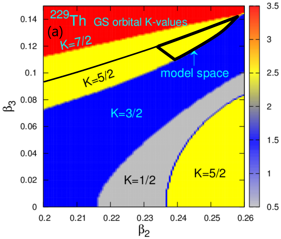
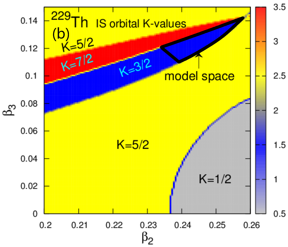
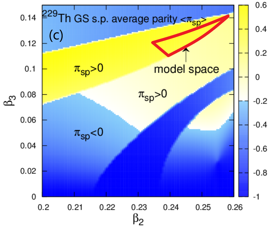
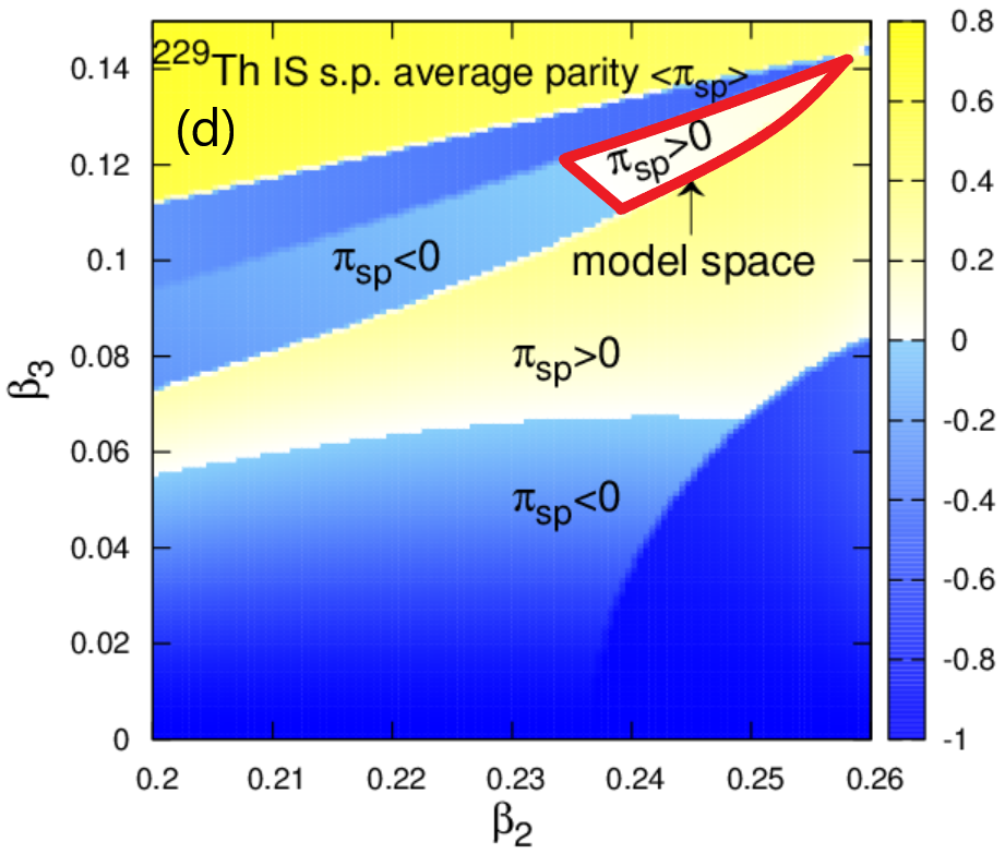
Figure 1: $K$-values for the (a) GS and (b) IS s.p. orbitals and the respective average parities (c), (d) $\langle\pi_{\mbox{\scriptsize sp}}\rangle$ appearing in the DSM within the space of quadrupole and octupole deformations. The regions of relevant deformations providing the correct $K_{GS}=5/2$ and $K_{IS}=3/2$ values with $\langle\pi_{\mbox{\scriptsize sp}}\rangle>0$ are delimitated by thick contour lines. The thinner black line in plot (a) maps the relevant border of the $K_{IS}=3/2$ region from plot (b).

The assumptions above sketch the mechanism which may lead to the formation of a quasidegenerate pair of $5/2^{+}$ GS and $3/2^{+}$ IS in ²²⁹Th. We see that the very fine interplay between the involved collective and s.p. degrees of freedom is directly governed by the Woods-Saxon DSM QO deformations $\beta_{2}$ and $\beta_{3}$, the pairing strength determined by the parameters $g_{0}$ and $g_{1}$ in Eq. (8) and the Coriolis mixing strength determined by the parameter $A$ in (3). The remaining CQOM parameters $\omega$, $b$, $d_{0}$, $c$ and $p$ influence the isomer energy through the overall fit of the energy spectrum, transition rates and magnetic moments. Within the above physical mechanism the $3/2^{+}$ IS of ²²⁹Th appears as an essentially s.p., i.e., microscopic, effect, the energy and electromagnetic properties of which, however, are formed under the influence of the collective dynamics of the nucleus.

In Ref. Minkov and Pálffy (2017) the above algorithm was applied through several steps, including the choice of $\beta_{2}$ and $\beta_{3}$ in DSM based on information available for neighbouring even-even nuclei (see the beginning of next section), tuning of the pairing constants in BCS to reach a rough proximity of GS and IS and subsequent fine adjustment of the collective CQOM parameters together with the $K$-mixing constant $A$ to obtain overall model description and predictions. It was demonstrated that at the expense of a minor deterioration of the agreement between the overall theoretical and experimental spectrum, one can exactly reproduce the IS energy of about 8 eV. Of course, such a refinement is of little practical significance since it is beyond the genuine accuracy provided by any nuclear structure model.

Few comments regarding the results in the next section should be given here in advance. We remark that some model parameters are not completely independent regarding particular physical observables. Thus, the change in the IS-GS displacement due to variation in the DSM QO deformations could be compensated by variations in the pairing constants or the $K$-mixing constant $A$. Therefore, one of the important issues to be clarified is the extent to which the different model parameters are correlated in the problem and how we can constrain them to reach most unambiguously the correct solution. Our numerical study showed that if we fix the pairing parameters in Eq. (8) to the values of $g_{0}=18.805$ MeV and $g_{1}=7.389$ MeV, which were tuned in the model description in Ref. Minkov and Pálffy (2017), the further analysis and drawn conclusions also apply for the pairing strengths adopted in Refs. Nilsson and Ragnarsson (1995) and Walker and Minkov (2010). Therefore, hereinafter we use the above fixed $g_{0}$ and $g_{1}$ parameter values while directing our study to the examination of the QO deformation space of the DSM. Another point is that in Ref. Minkov and Pálffy (2019) the IS and GS magnetic moments were predicted without taking their experimental values into the model adjustment procedure. In the present work we include the magnetic moments into the fitting procedure by considering all observables in the fit analysis (energies, transition rates and magnetic moments) on the same footing. We will also investigate to what extent the gyromagnetic quenching factors $q_{s}$ and $q_{R}$ can be reasonably varied for the reproduction of the GS and IS magnetic moments. This analysis aims to reduce the arbitrariness in the model predictions for the ²²⁹Th IS properties.

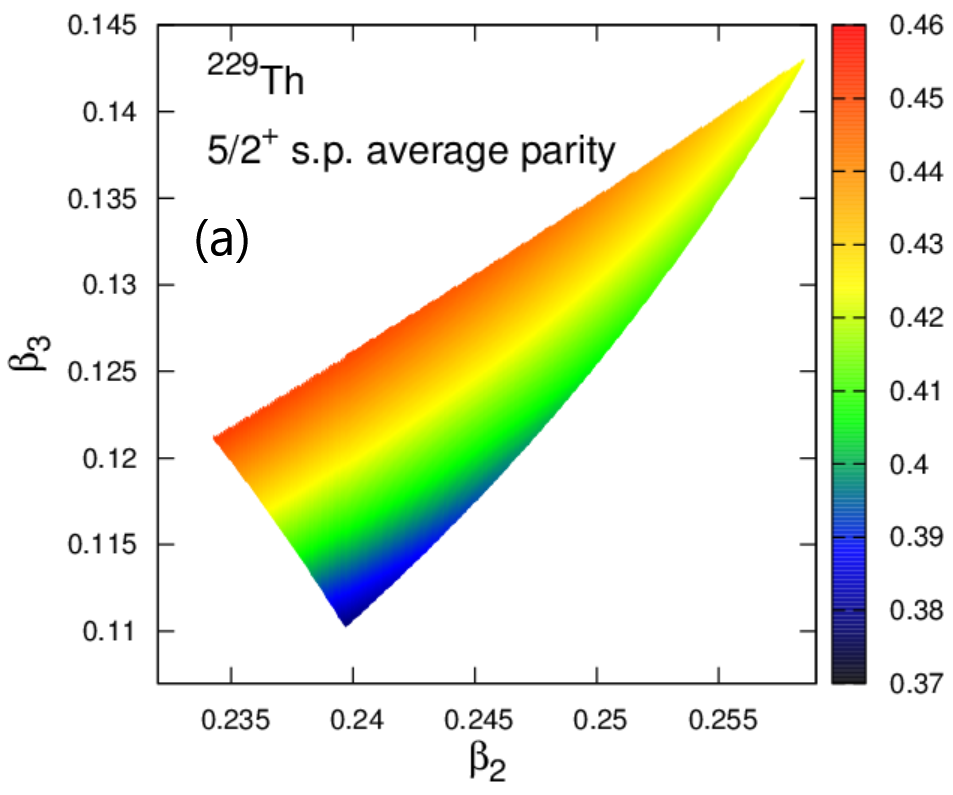
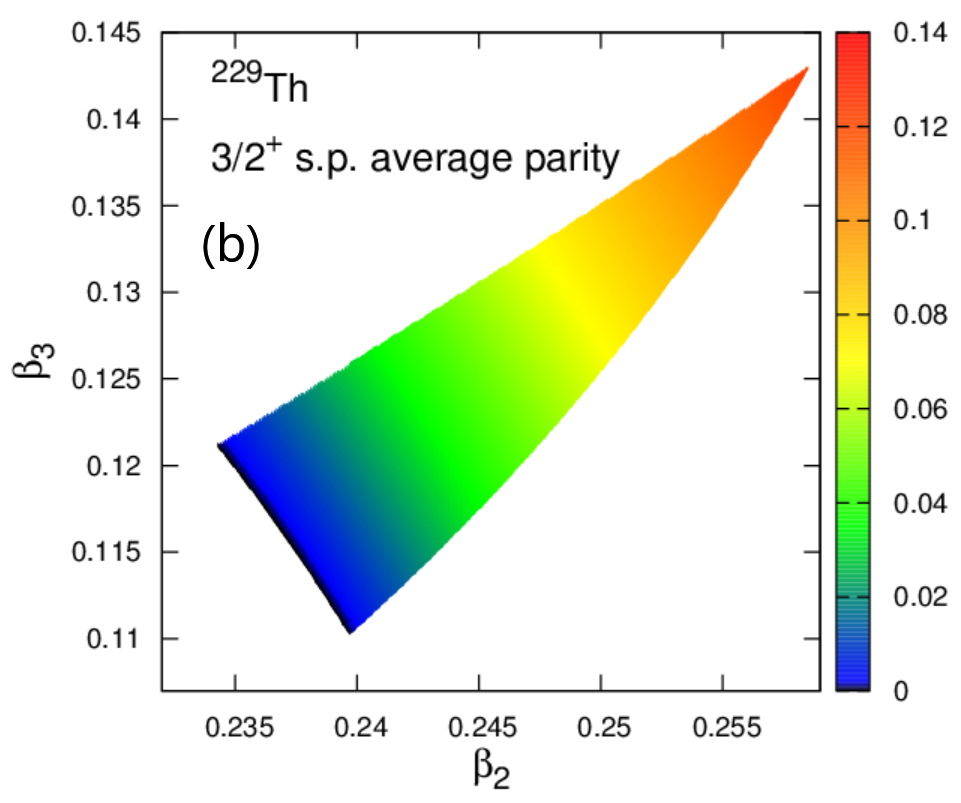
Figure 2: Average parity $\langle\pi_{\mbox{\scriptsize sp}}\rangle$ in the (a) GS and (b) IS s.p. orbitals appearing in DSM within the model-defined QO deformation space.

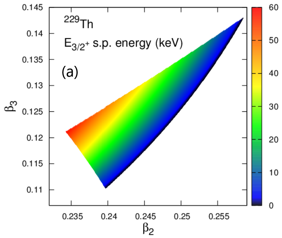
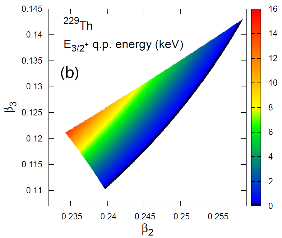
Figure 3: (a) S.p. and (b) q.p. energy (in keV) of the $3/2^{+}$ isomer orbital with respect to the $5/2^{+}$ GS orbital appearing in DSM within the model-defined space of QO deformations. The q.p. energy is obtained with pairing parameters $g_{0}=18.805$ MeV and $g_{1}=7.389$ MeV used in Eq. (8). See text for further explanations.

III Numerical results and discussion

III.1 Determination of the deformed shell model deformation space

The Woods-Saxon DSM shape parameters $\beta_{2}$ and $\beta_{3}$ represent a basic input of our model and their values are decisive for the model predictions. Hereafter under “QO deformations and/or parameters” we will understand these two quantities unless otherwise specified. In Ref. Minkov and Pálffy (2017) the quadrupole-deformation parameter $\beta_{2}$ was chosen by varying it between the experimental values 0.230 and 0.244 available for the neighbouring even-even nuclei ²²⁸Th and ²³⁰Th, respectively Raman et al. (2001). Simultaneously the octupole-deformation parameter $\beta_{3}$ was varied to obtain the GS and IS orbitals very close to each other, with leading 5/2[633] and 3/2[631] components in the respective s.p. wave-function expansions given in Eq. (6), and with positive average values of the parity $\langle\pi_{\mbox{\scriptsize sp}}\rangle>0$ from Eq. (7) in both s.p. states. We note that the chosen interval for the octupole deformation was at that time solely relying on model estimates. However, in the meantime we have found out that this range is also supported by an independent microscopic result. In Ref. Nomura et al. (2014) self-consistent relativistic Hartree-Bogoliubov model calculations with the universal energy density functional DD-PC1 Nikšić et al. (2008) predict a rather deep total-energy minima for $\beta_{3}$ between 0.1 and 0.2 in the neighboring even-even nuclei ²²⁸Th and ²³⁰Th.

In this study we identify the ($\beta_{2},\beta_{3}$) deformation space which could provide a relevant model description of the ^229mTh isomer similar to the one obtained in Refs. Minkov and Pálffy (2017, 2019) which had considered the values $\beta_{2}=0.240$ and $\beta_{3}=0.115$. To this end we have performed DSM calculations on a grid in the ranges $0.2\leq\beta_{2}\leq 0.26$ and $0\leq\beta_{3}\leq 0.15$ which are supposed to include the QO deformations physically relevant for a nucleus in the mass region of ²²⁹Th. At each point of the grid we obtain the $K$-value and the average parity $\langle\pi_{\mbox{\scriptsize sp}}\rangle$ for the last occupied s.p. orbital, which is supposed to determine the GS and for the next (first) non-occupied orbital, candidate for the IS. Note that the calculation does not involve the collective (CQOM) part of the model and the only entering parameters are the two Woods-Saxon DSM deformations.

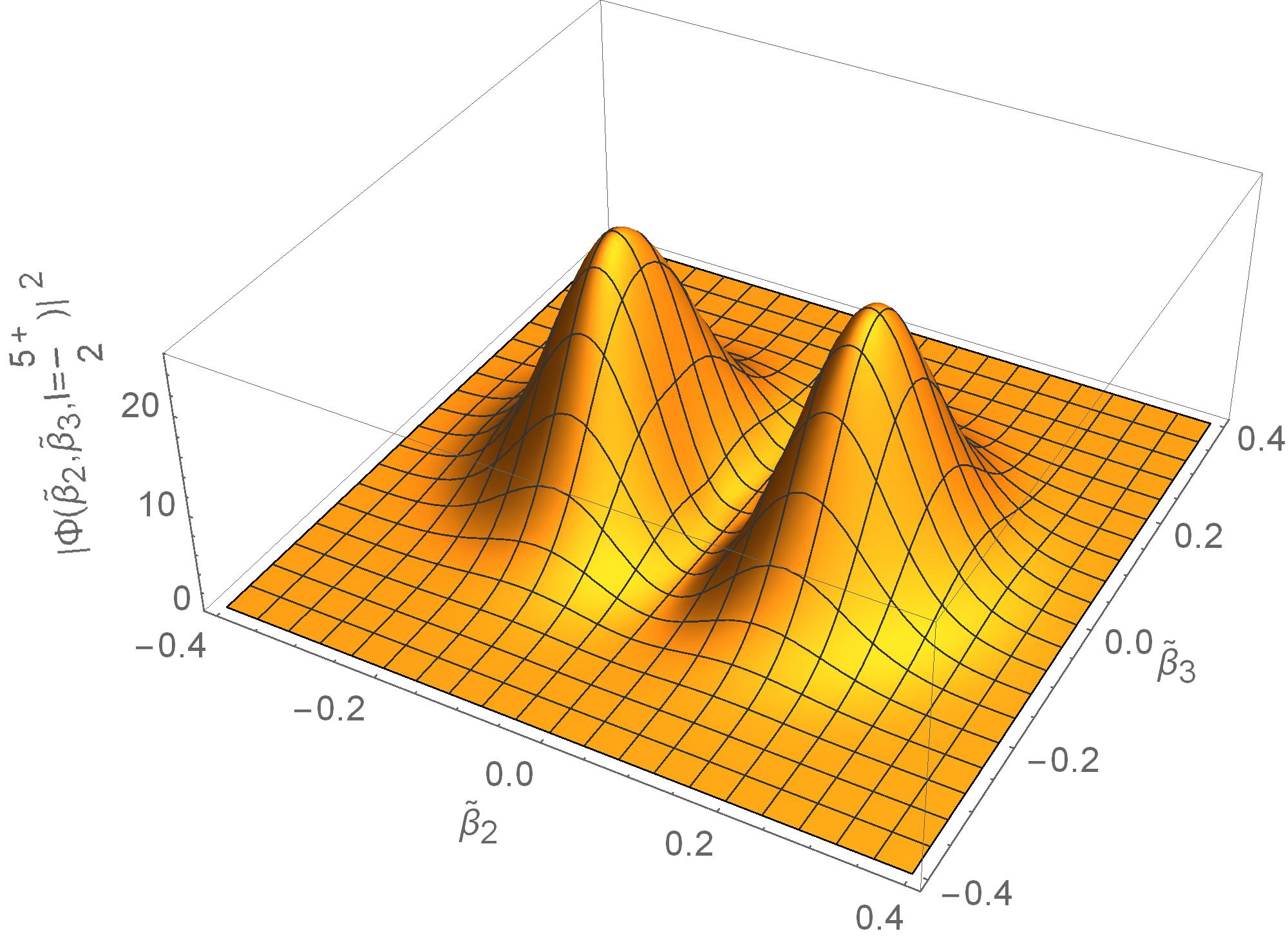
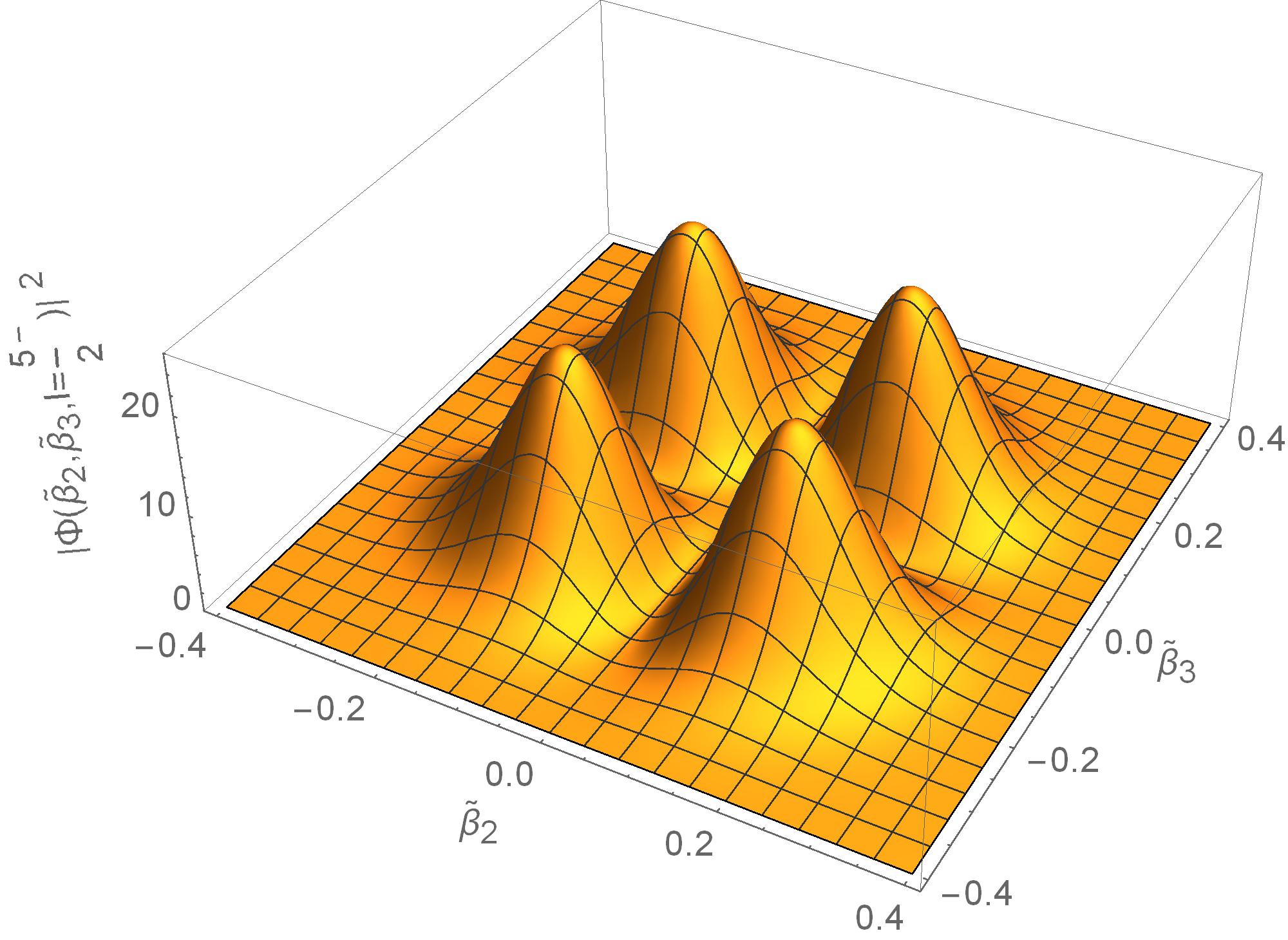
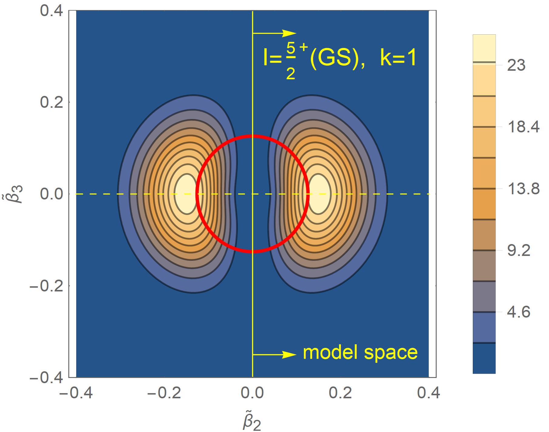
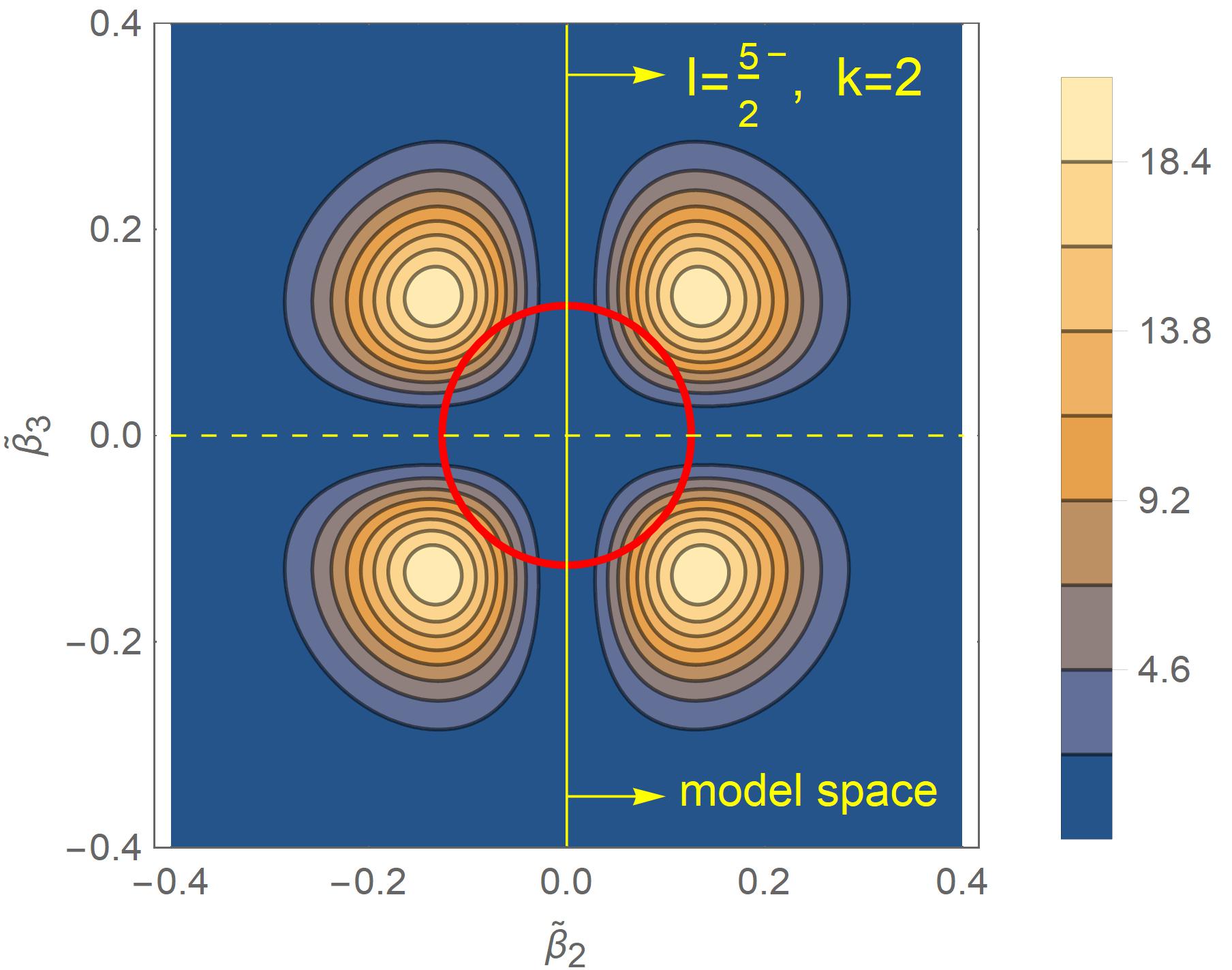
Figure 4: The CQOM QO wave-function density $|\Phi^{\pi_{\mbox{\scriptsize qo}}}_{nkI}(\tilde{\beta_{2}},\tilde{\beta_{3}})|^{2}$ from Eq. (15) as a function of $\tilde{\beta}_{2}$ and $\tilde{\beta}_{3}$ for the $I^{\pi}=5/2^{+}$ GS (with $k=1$) and $5/2^{-}$ state (with $k=2$) of the yrast quasi-parity-doublet in ²²⁹Th. We use here the DSM+CQOM fit with $q_{s}=q_{R}=0.6$ and the Woods-Saxon DSM deformation parameters ($\beta_{2},\beta_{3}$)=($0.240,0.115$). The upper panels represent three-dimensional plots while the lower panels illustrate the corresponding projected two-dimensional contour plots. The CQOM potential bottoms defined by the semiaxes $\tilde{\beta}_{2,3}^{\mbox{\scriptsize sa}}$ are shown as red circles.

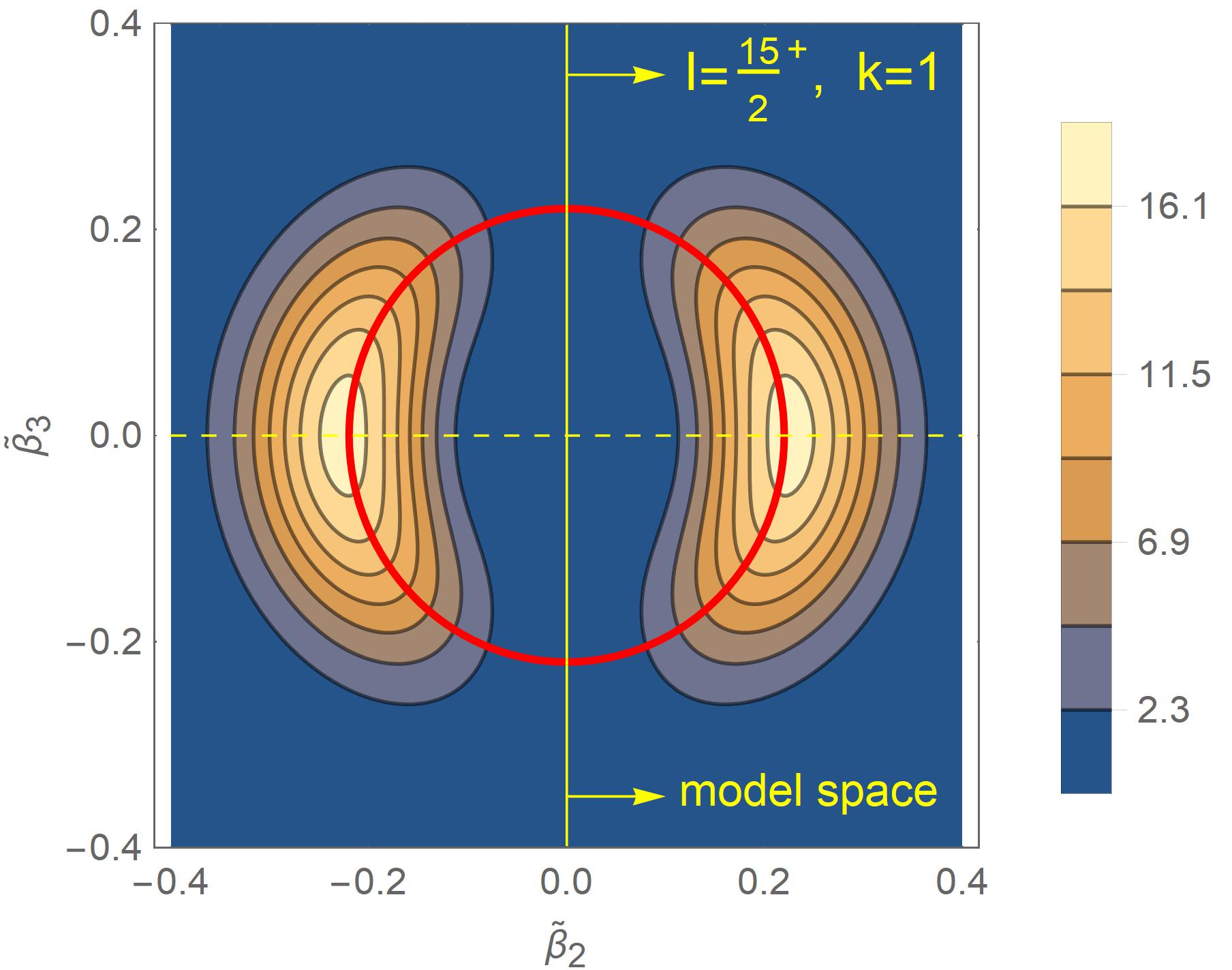
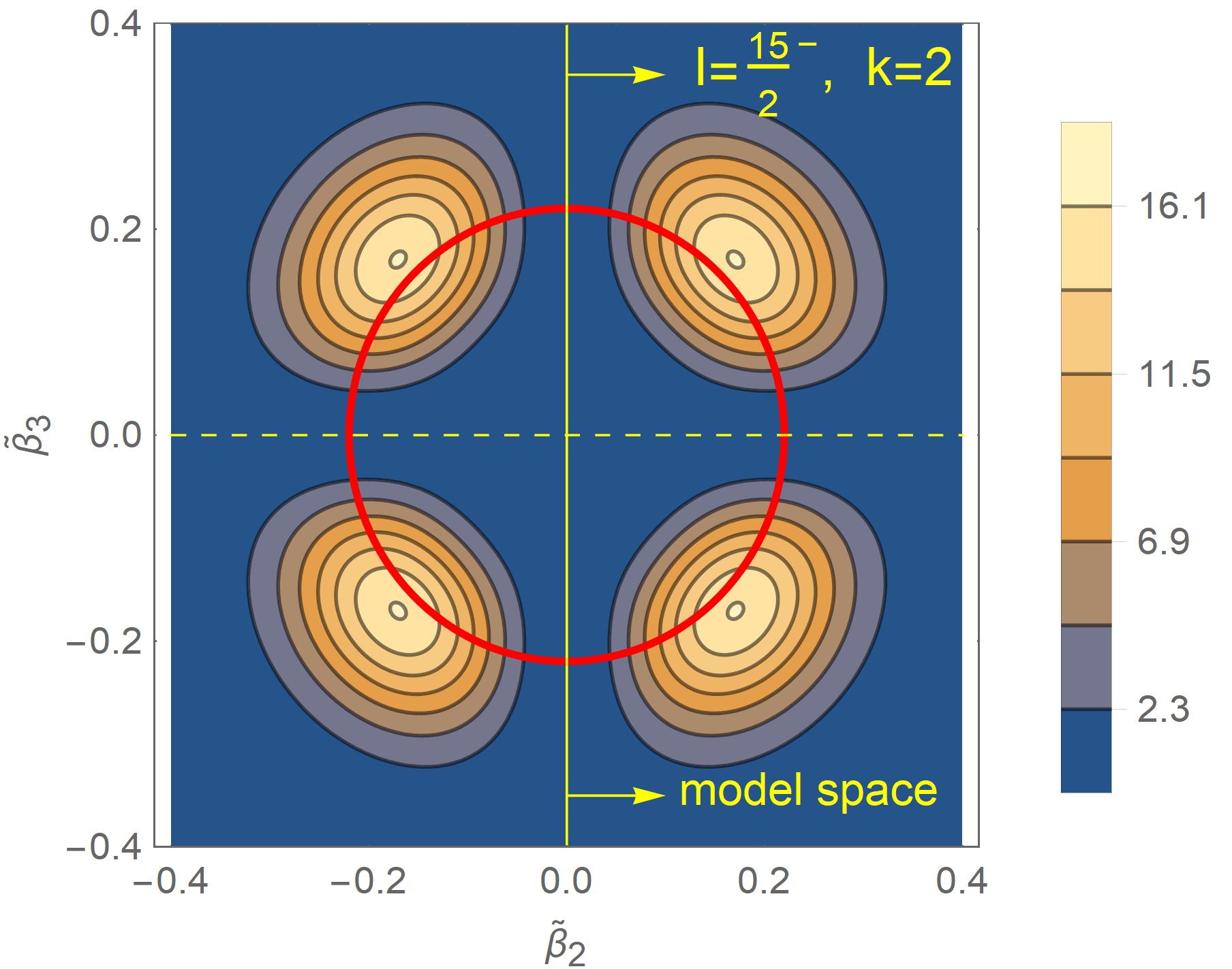
Figure 5: The same as Fig. 4 (lower panels), but for the $I^{\pi}=15/2^{+}$ and $15/2^{-}$ yrast quasi-parity-doublet states of ²²⁹Th. Note the considerable increase in the QO semiaxes and the corresponding expansion of the dynamical-deformation peak positions in the space of the collective CQOM variables $\tilde{\beta}_{2}$ and $\tilde{\beta}_{3}$.

The result of this calculation is shown in Fig. 1. Figs. 1 (a) and 1 (b) present in color coding the $(\beta_{2},\beta_{3})$ areas in which different $K$ values appear for the GS and IS orbitals, respectively. For the GS orbital the $K=5/2$ value appears in two (yellow) regions, while for the IS the $K=3/2$ value appears in one narrow (blue) region. The intersection of the $K=5/2$ GS and $K=3/2$ IS subspaces coincides with the blue $K=3/2$ region for the IS and depicts the ($\beta_{2},\beta_{3}$)- region in which the DSM provides the required 5/2[633] and 3/2[631] orbitals for the GS and IS, respectively. Furthermore, considering the information from Fig. 1 (c) and 1 (d), one can identify in a similar way the regions with positive and negative average values of the parity in the GS and IS orbitals, respectively. By retaining only the $\langle\pi_{\mbox{\scriptsize sp}}\rangle>0$ areas for both orbitals, one ends up with a rather limited ($\beta_{2},\beta_{3}$)-region given by the thick triangle contour in the four plots. This region includes all QO deformations from the considered space which are relevant within the DSM regarding the current experimental information and theoretical interpretation of the $K^{\pi}=3/2^{+}$ isomer in ²²⁹Th. Hereinafter we call this region our “model deformation space”.

Based on the above result, we can draw the following important conclusion. Considering the long-adopted $K$-value and parity of the ^229mTh IS, our DSM prediction shows that this isomer can only exist at essentially nonzero octupole deformation of the s.p. potential. More precisely, one can say that the coexistence of the $K^{\pi}=3/2^{+}$ IS together with the $K^{\pi}=5/2^{+}$ GS requires the presence of nonzero octupole deformation, as seen from Fig. 1(a). In fact our more extended calculations in the QO deformation grid show that for $\beta_{2}<0.2$ the (yellow) range of coexisting $K^{\pi}=5/2^{+}$ GS and $K^{\pi}=3/2^{+}$ IS orbitals goes down and further reaches the $\beta_{3}=0$ line. However, this occurs around $\beta_{2}\sim 0.1$, which is far beyond the deformation limits typical for this mass region. Thus, we can conclude that the octupole deformation appears to be of a crucial importance for the formation of the ^229mTh isomer according to the present knowledge on the corresponding GS and IS angular momenta and parities.

Furthermore, we note that the deformation values ($\beta_{2}=0.240,\beta_{3}=0.115$) used in Refs. Minkov and Pálffy (2017, 2019) appear close to the lowest vertex of the investigated DSM deformation space. The relatively small area of this space suggests a reasonable degree of arbitrariness in the model conditions imposed in the studies of Refs. Minkov and Pálffy (2017) and Minkov and Pálffy (2019) regarding the choice of QO deformation. Moreover, the deformation region determined in this work appears to be consistent with the corresponding areas of the QO minima in the energy surfaces of ²²⁸Th and ²³⁰Th obtained in the relativistic Hartree-Bogoliubov model calculations Nomura et al. (2014). Nevertheless, the precise determination and prediction of the ^229mTh isomer properties as well as the deeper understanding of the mechanism governing its formation requires a more detailed examination of the model descriptions obtained for various deformations fixed in the outlined model space. In the following our study is focused on this task.

A direct consequence of the location of the model space at nonzero octupole deformation is that the GS and IS s.p. orbitals provided by the DSM always appear with mixed parity which has to be projected in the total core plus particle wave function, as seen in Eq. (20), and implemented in the model procedure applied in Minkov and Pálffy (2017). The average parity $\langle\pi_{\mbox{\scriptsize sp}}\rangle$ of both orbitals calculated from Eq. (7) as a function of the QO deformations within the model space is illustrated in Fig. 2. The results show that while in the GS the quantity $\langle\pi_{\mbox{\scriptsize sp}}\rangle$ varies within the limits $0.37-0.46$, in the IS the parity mixing is even much stronger with $\langle\pi_{\mbox{\scriptsize sp}}\rangle$ varying between 0 and 0.14. The black side of the triangle in Fig. 2(b) corresponds to the (left) border of the space where the average parity of the IS turns from positive to negative values. This result shows that the mechanism governing the formation of the isomer is even more complicated due to the fine parity-mixed structure of the s.p. wave functions and the accordingly applied projection procedure.

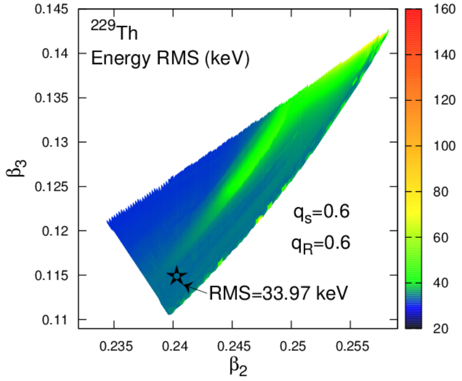
Figure 6: Energy RMS values in keV for the GS (yrast) and IS (excited) bands together obtained by the model fit on a grid within the model-defined QO deformation space. We use $q_{s}=q_{R}=0.6$. The open star indicates the location of the deformations ($\beta_{2},\beta_{3}$)=($0.240,0.115$) adopted in Refs. Minkov and Pálffy (2017, 2019).

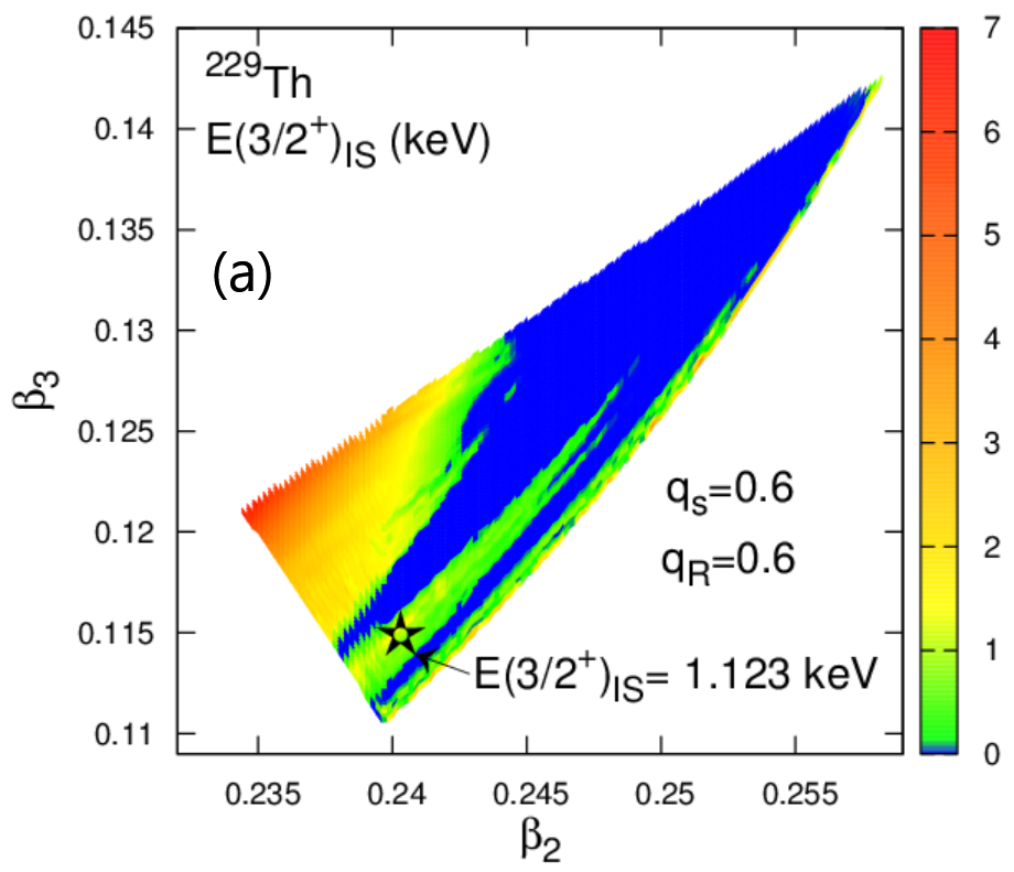
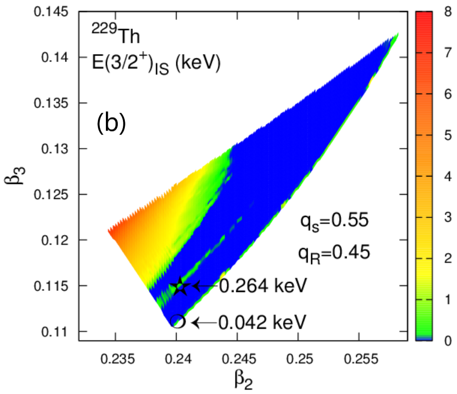
Figure 7: Isomer energy $E_{IS}$ obtained by the model fits on a model-defined QO deformation space grid for two different combinations of $q_{s}$ and $q_{R}$. The open star indicates the location of the deformations ($\beta_{2},\beta_{3}$)=($0.240,0.115$) adopted in Refs. Minkov and Pálffy (2017, 2019). The circle indicates the set ($\beta_{2},\beta_{3}$)=($0.240,0.111$) situated closer to the degeneracy line.

Other important quantities delivered by the DSM are the s.p. and q.p. energies for the IS orbital determined with respect to the corresponding energies in the GS orbital, $E^{\mbox{\scriptsize sp}}_{3/2^{+}}=E_{\mbox{\scriptsize sp}}^{3/2^{+}}-E_{\mbox{\scriptsize sp}}^{5/2^{+}}$ and $E^{\mbox{\scriptsize qp}}_{3/2^{+}}=\epsilon_{\mbox{\scriptsize qp}}^{3/2^{+}}-\epsilon_{\mbox{\scriptsize qp}}^{5/2^{+}}$. The lowering of the q.p. energy with respect to the s.p. energy can be controlled through additional tuning of the pairing constants as shown in Ref. Minkov and Pálffy (2017). However, as argued at the end of Sec. II.5, here we use the $g_{0}$ and $g_{1}$ values fixed in Minkov and Pálffy (2017) focusing our analysis on the deformation dependencies. In Fig. 3 both $E^{\mbox{\scriptsize sp}}_{3/2^{+}}$ and $E^{\mbox{\scriptsize qp}}_{3/2^{+}}$ for the IS are plotted as functions of $\beta_{2}$ and $\beta_{3}$. As expected, they show an identical dependence but with different nominal values. In addition, along the right side of the triangle the q.p. and s.p. content of the isomer energy goes to zero, i.e. the two orbitals, 5/2[633] and 3/2[631] mutually degenerate. This is an important limit of the model deformation space. In fact the black lines in Fig. 3 correspond to the crossing of both orbitals when leaving the model space to enter the blue area with $K=3/2$ in Fig. 1(a) and the lower $K=5/2$ (yellow) area in Fig. 1(b), a situation in which the GS appears with $K^{\pi}=3/2^{+}$ and the IS obtains $K^{\pi}=5/2^{+}$. The proximity to this line from the model space interior determines the degree of the q.p. quasidegeneracy effect. For the pair of QO deformations ($\beta_{2},\beta_{3}$)=($0.240,0.115$) adopted in Refs. Minkov and Pálffy (2017, 2019), the $3/2^{+}$ q.p. energy yields $E^{\mbox{\scriptsize qp}}_{3/2^{+}}=2.196$ keV. We note that this is not the final IS energy in which additional contributions take a part as explained in Sec. II.5. The upper side of the triangle corresponds to the crossing of the $K^{\pi}=3/2^{+}$ orbital with a $K^{\pi}=7/2^{-}$ orbital with leading component 7/2[743] [see red area in Fig. 1(b)]. It is not of a particular interest from the isomer-formation point of view.

III.2 Coherent quadrupole-octupole model fits in the deformed shell model deformation space

At this point we are ready to examine the behaviour of the model description and prediction for the physical observables of interest within the DSM deformation space. We are especially interested in the corresponding behaviour of the $B(M1)$ and $B(E2)$ IS transition rates and of the IS and GS magnetic moments $\mu_{\mbox{\scriptsize GS}}$ and $\mu_{\mbox{\scriptsize IS}}$. To this end we have performed full model fits by adjusting the five CQOM parameters, $\omega$, $b$, $d_{0}$, $c$, $p$ and the Coriolis mixing constant $A$ with respect to the experimental quasi-parity-doublet spectrum, the available transition rates and magnetic moments at each point of the deformation space grid with the pairing constants fixed as described above. Thus, for each pair of Woods-Saxon DSM QO deformations we obtain the full spectroscopic description of the nucleus storing the quantities of interest for our systematic analysis presented below.

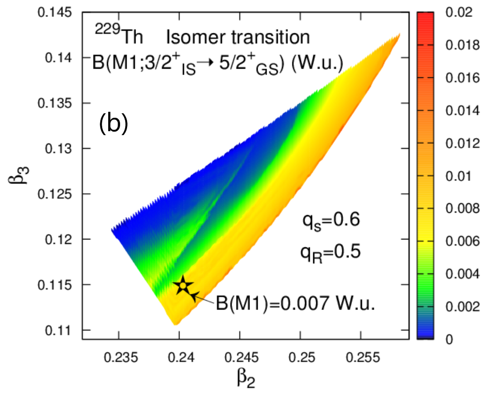
Figure 8: $B(M1)$ isomer transition values obtained by the model fits on a grid within the model-defined QO deformation space at four different combinations of $q_{s}$ and $q_{R}$. The open star indicates the location of the deformations ($\beta_{2},\beta_{3}$)=($0.240,0.115$) adopted in Refs. Minkov and Pálffy (2017, 2019). The circle in panel (d) indicates the set ($\beta_{2},\beta_{3}$)=($0.240,0.111$) situated closer to the degeneracy line.

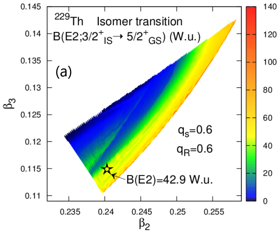
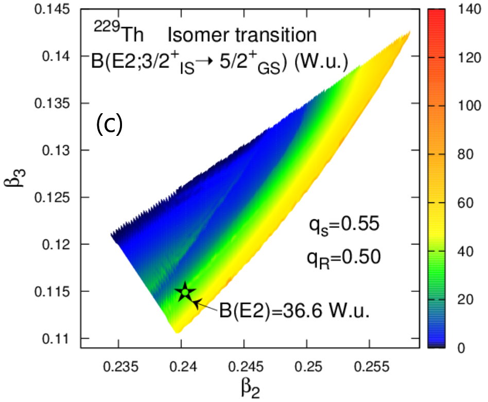
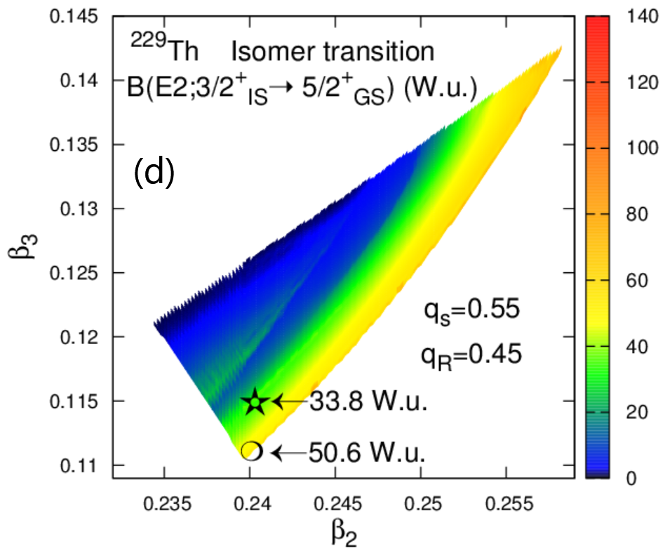
Figure 9: $B(E2)$ isomer transition values obtained by the model fits on the model-defined QO deformation space grid at four different combinations of $q_{s}$ and $q_{R}$. The open star indicates the location of the deformations ($\beta_{2},\beta_{3}$)=($0.240,0.115$) adopted in Refs. Minkov and Pálffy (2017, 2019). The circle in panel (d) indicates the set ($\beta_{2},\beta_{3}$)=($0.240,0.111$) situated closer to the degeneracy line.

The five adjusted CQOM parameters show a smooth behavior along the deformation space with values consistent with those obtained in Ref. Minkov and Pálffy (2017). We therefore refrain from addressing further numerical details here. We note however that the parameter $p$ defined in Eq. (11) is close to unity $p\approx 1$ throughout the entire DSM ($\beta_{2},\beta_{3}$)-model space. This parameter indicates the relative contribution of the quadrupole and octupole modes in the CQOM. Thus, according to Eq. (14) all parameter fits lead to a practically circular bottom of the CQOM potential with $\tilde{\beta}_{2}^{\mbox{\scriptsize sa}}\approx\tilde{\beta}_{3}^{\mbox{\scriptsize sa}}$, showing that the model describes the collective quasi-parity-doublet structure of the ²²⁹Th spectrum with equal weights of the quadrupole $\tilde{\beta}_{2}$ and octupole $\tilde{\beta}_{3}$ deformation modes. Considering the DSM deformation parameters $\beta_{2}=0.240$ and $\beta_{3}=0.115$ used in Ref. Minkov and Pálffy (2017), we obtain for the $5/2^{+}$ GS and $3/2^{+}$ IS states values between 0.12 and 0.17 for the two equal $\tilde{\beta}_{2,3}^{\mbox{\scriptsize sa}}$ semiaxes (which define the circle radius of the CQOM potential bottom).

Inspection of the odd-nucleon contribution to $\tilde{\beta}_{2,3}^{\mbox{\scriptsize sa}}$ determined in Eq. (13) through Eq. (3) at ($\beta_{2},\beta_{3}$)=($0.240,0.115$) shows that in the case of ²²⁹Th the Coriolis mixing causes a negligible decrease in $\tilde{\beta}_{2,3}^{\mbox{\scriptsize sa}}$ compared with the core case, Eq. (12), while a considerable decrease is caused by the term $(-K_{b}^{2})$. Thus while in the core+particle case the GS $\tilde{\beta}_{2,3}^{\mbox{\scriptsize sa}}=0.122$, for the core only [without the term $(-K_{b}^{2})$] these values become 0.149. Similarly, in the isomeric state the core+particle $\tilde{\beta}_{2,3}^{\mbox{\scriptsize sa}}=0.121$, while in the core case the semiaxes values rise to 0.132. Figure 4 illustrates the CQOM QO wave-function densities $|\Phi^{\pi_{\mbox{\scriptsize qo}}}_{nkI}(\tilde{\beta_{2}},\tilde{\beta_{3}})|^{2}$ from Eq. (15) for the $I^{\pi}=5/2^{+}$ GS and its negative-parity counterpart $5/2^{-}$ obtained with the parameters of the CQOM fit at ($\beta_{2},\beta_{3}$)=($0.240,0.115$). For simplicity we have only taken into account the $(-K_{b}^{2})$ term in $\widetilde{X}(I^{\pi},K_{b})$ dropping the negligible Coriolis mixing term. The wave function density was calculated for the quenching parameter set ($q_{s},q_{R}$)=($0.6,0.6$). The dynamical deformations are indicated by the positions of the density maxima in the Figure. We see that in the two states these deformations appear outside of the potential bottom circle. Furthermore, the dynamical deformation parameters are not coinciding with the DSM ($\beta_{2},\beta_{3}$) parameters, confirming the discussion in Sec. II.2 on the distinction between dynamical deformation parameters in the CQOM and the DSM deformation parameters. We also note that the CQOM potential bottom semiaxes $\tilde{\beta}_{2,3}^{\mbox{\scriptsize sa}}$ (the red circles) do not change between the positive- and negative-parity counterparts in the quasi-parity-doublet since the Coriolis mixing term only mixes states with the same (bandhead) parity. This situation, however, would be different in a spectrum build on the $K_{b}=1/2$ bandhead (which is not present for the case of ²²⁹Th) where the decoupling term in $\widetilde{X}(I^{\pi},K_{b})$ in Eq. (3) would act in opposite directions on the semiaxes lengths of the opposite-parity counterparts.

We have checked that the density plots for the $I^{\pi}=3/2^{+}$ IS and its $3/2^{-}$ quasi-parity-doublet counterpart (not given here) look very similar to those in Fig. 4. To investigate the effect of higher angular momentum values we show the CQOM QO wave-function densities for the $I=15/2^{\pm}$ states of the yrast quasi-parity-doublet in Fig. 5. The CQOM potential semiaxes $\tilde{\beta}_{2,3}^{\mbox{\scriptsize sa}}$ and the corresponding dynamical deformations considerably increase with angular momentum, reaching at $I=15/2^{\pm}$ values larger than $0.2$. This shows that the dynamical deformation is responsible for the higher-energy part of the spectrum which otherwise would not be felt by the s.p. potential. We may conclude that the model algorithm rather carefully takes into account also the influence of the collective dynamics at the higher angular momenta, which reflects on the overall deformation characteristics of the CQOM potential.

Finally, special attention is given below to the behaviour of the Coriolis mixing constant $A$ which, as already mentioned, plays an important role in the formation of the IS energy and electromagnetic properties. The calculations were repeated for four pairs of ($q_{s},q_{R}$) values of the quenching factors considered for the spin and collective gyromagnetic rates. As the analysis of magnetic moments made in Ref. Minkov and Pálffy (2019) suggests the need of rather strong attenuation of the latter, here we consider $q_{s}$ and $q_{R}$ with slightly lower values compared with the lowest pair ($q_{s},q_{R}$)=($0.6,0.6$) considered in Ref. Minkov and Pálffy (2019). Thus, in the present calculations the gyromagnetic quenching factors were allowed to be as small as ($q_{s},q_{R}$)=($0.55,0.45$). Although the experimental value of the isomeric energy is obviously out of reach for the model accuracy, we also consider its theoretical prediction $E(3/2^{+})_{IS}$ in order to see how the model fits “feel” its tiny energy scale as well as to assess accordingly the relevance of the overall model description for the different deformations within the model space.

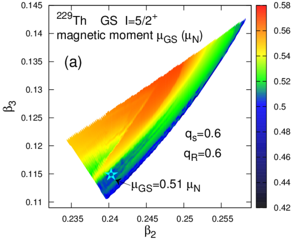
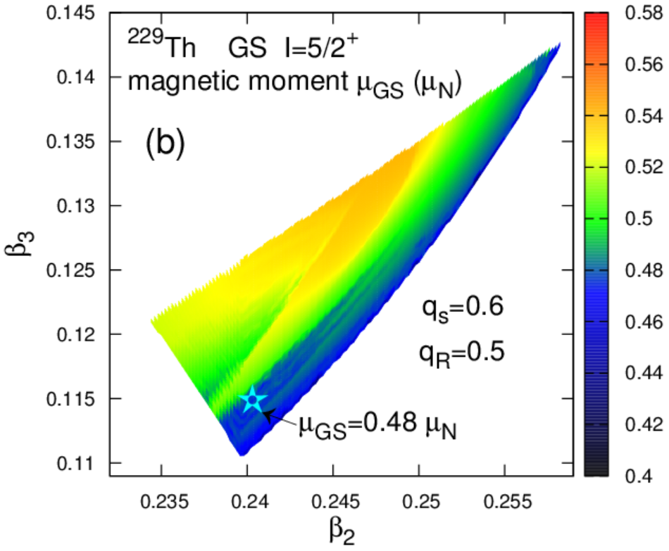
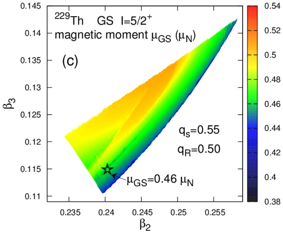
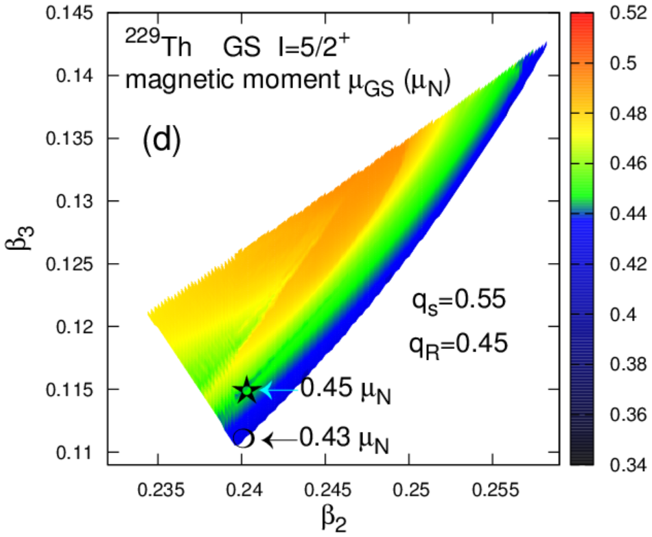
Figure 10: GS magnetic moment values obtained by the model fits on a grid within the model-defined QO deformation space at four different combinations of $q_{s}$ and $q_{R}$. The open star and the circle indicate the same sets of deformations as shown in Figs. 8 and 9.

III.3 Energy description

The primary quantity providing overall information about the relevance of the model descriptions in the different points of the deformation space is the root-mean-square (RMS) deviation between the theoretical and experimental energy levels. Its behaviour as a function of the DSM QO deformation for calculations made with quenching factors ($q_{s},q_{R}$)=($0.6,0.6$) is illustrated in Fig. 6. We indicate with an open star the location of the deformations ($\beta_{2},\beta_{3}$)=($0.240,0.115$), adopted in Refs. Minkov and Pálffy (2017, 2019). The RMS value obtained in this point is about 34 keV which is the same as the value obtained in the original model fits performed in Minkov and Pálffy (2017), although now the experimental values of the magnetic moments $\mu_{\mbox{\scriptsize GS}}$ and $\mu_{\mbox{\scriptsize IS}}$ are included in the fits. We note that the RMS factor is close to this value over a larger area of the deformation model space, demonstrating the stability of the model solutions with the variation of QO deformations. The upper part of the space with large $\beta_{2}$ and $\beta_{3}$ values, however, appears unfavoured. We have verified that in all regions of the space with the RMS close to 34 keV the description of the overall energy spectrum and the available $B(M1)$ and $B(E2)$ transition rates is of similar accuracy as the one reported in Ref. Minkov and Pálffy (2017), with the obtained CQOM parameter values being close to those in Ref. Minkov and Pálffy (2017) (see Fig. 1 and Table 1 therein). We notice that in the upper-left parts of the plot some lower RMS deviations are obtained as low as $\approx$30 keV, however, for these deformations the model predictions for the isomer energy are less favourable as analyzed below. In addition, we found (barely visible in Fig. 6) that towards the line of the 5/2[633]–3/2[631] degeneracy the RMS factor sharply increases. As discussed below in relation to the particular observables, this is the result of the strong increase of the Coriolis $K$-mixing interaction which largely exceeds the perturbation theory limitation and puts a constraint on the model description valid close to the $5/2^{+}$–$3/2^{+}$ orbital crossing.

In Fig. 7 the theoretical isomer energy values $E_{IS}$ obtained by the model fits on the DSM QO space grid are presented for two sets of gyromagnetic quenching values $(q_{s},q_{R})=(0.6,0.6)$ and ($0.55,0.45$). We find that for the first set the value obtained at the pair of deformations ($\beta_{2},\beta_{3}$)=($0.240,0.115$) is $E_{IS}\approx 1$ keV, whereas for the second set it is $E_{IS}\approx 0.3$ keV. For the second set we choose to demonstrate the result for one more pair of deformations from our grid ($\beta_{2},\beta_{3}$)=($0.2398,0.1108$), further on denoted for simplicity by the rounded values ($0.240,0.111$), situated closer to the degeneracy line. There we have $E_{IS}\approx 0.040$ keV already approaching the scale of the experimental value. We note that for this pair of deformations the $3/2^{+}$ q.p. energy yields $E^{\mbox{\scriptsize qp}}_{3/2^{+}}=0.188$ keV.

All $E_{IS}$ values shown in Fig. 7 are obtained in the fitting procedure on the same footing without particular refinement. As already mentioned, one can easily achieve the exact experimental value of 0.008 keV through a very fine tuning of model parameters (e.g. the $K$-mixing $A$), with a minimal deterioration of the description in the remaining energy levels (see also Ref. Minkov and Pálffy (2017)). The plots in Fig. 7 show that in the large areas of the model space the fits provide reasonable values of $E_{IS}$ which could be renormalized to the experiment in this manner. However, we also see that in the upper-left parts of the plots the $E_{IS}$ considerably increases up to 7-8 keV giving an indication that at these deformations the remoteness of the 5/2[633] and 3/2[631] orbitals (see Fig. 3) already makes it difficult for the model mechanism to achieve quasidegeneracy. Also, we notice a thin stripe with large $E_{IS}$ values along the line of degeneracy which obviously indicates the limitation of the perturbation theory. Concluding this part, our analysis of the RMS factor and isomer energy values outlines certain limits of reliability of the present model application and favours the lower vertex of the model space around the deformation set used in Ref. Minkov and Pálffy (2017) in reasonable proximity to the $5/2^{+}$–$3/2^{+}$ orbitals crossing line.

III.4 $B(M1)$ and $B(E2)$ isomer transition rates

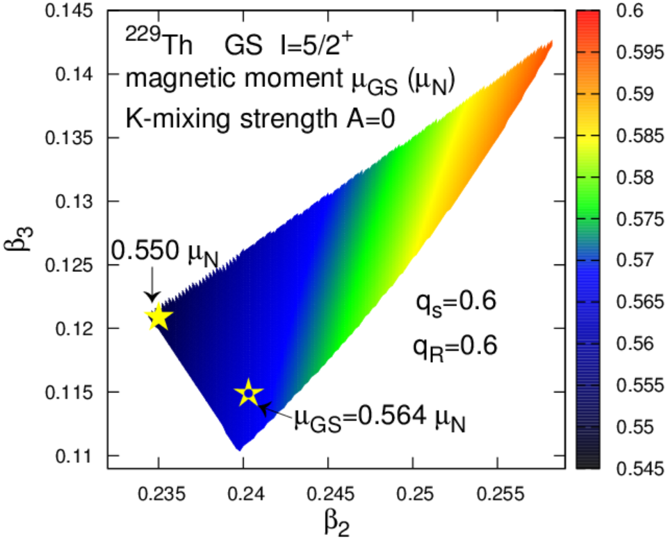
Figure 11: The “bare” s.p. GS magnetic moment values obtained without Coriolis mixing ($A=0$) on a grid within the model-defined QO deformation space with $q_{s}=q_{R}=0.6$. The open star indicates the location of the deformations ($\beta_{2},\beta_{3}$)=($0.240,0.115$) adopted in Refs. Minkov and Pálffy (2017, 2019). The full star indicates the grid point which provides the lowest value $\mu_{\mbox{\scriptsize GS}}$=0.55 $\mu_{N}$.

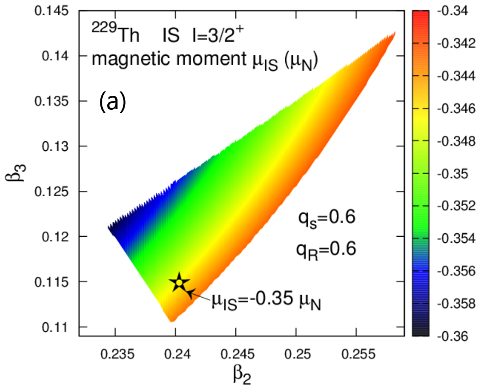
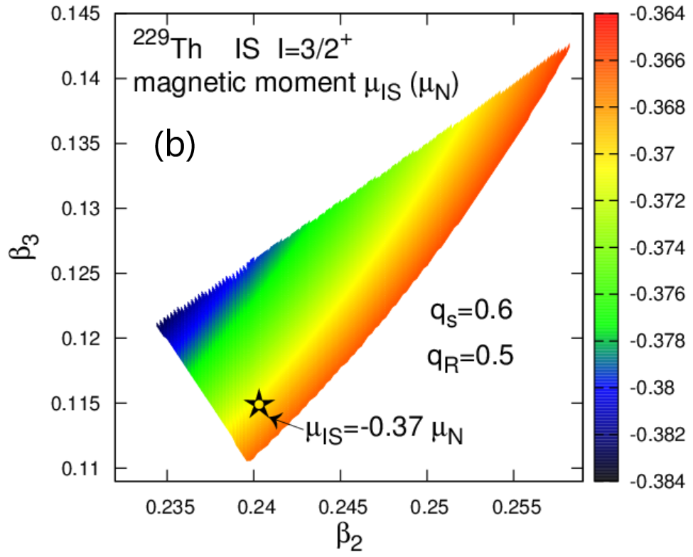
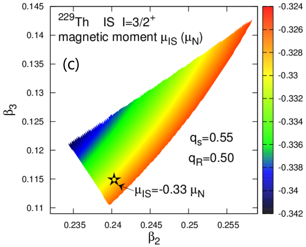
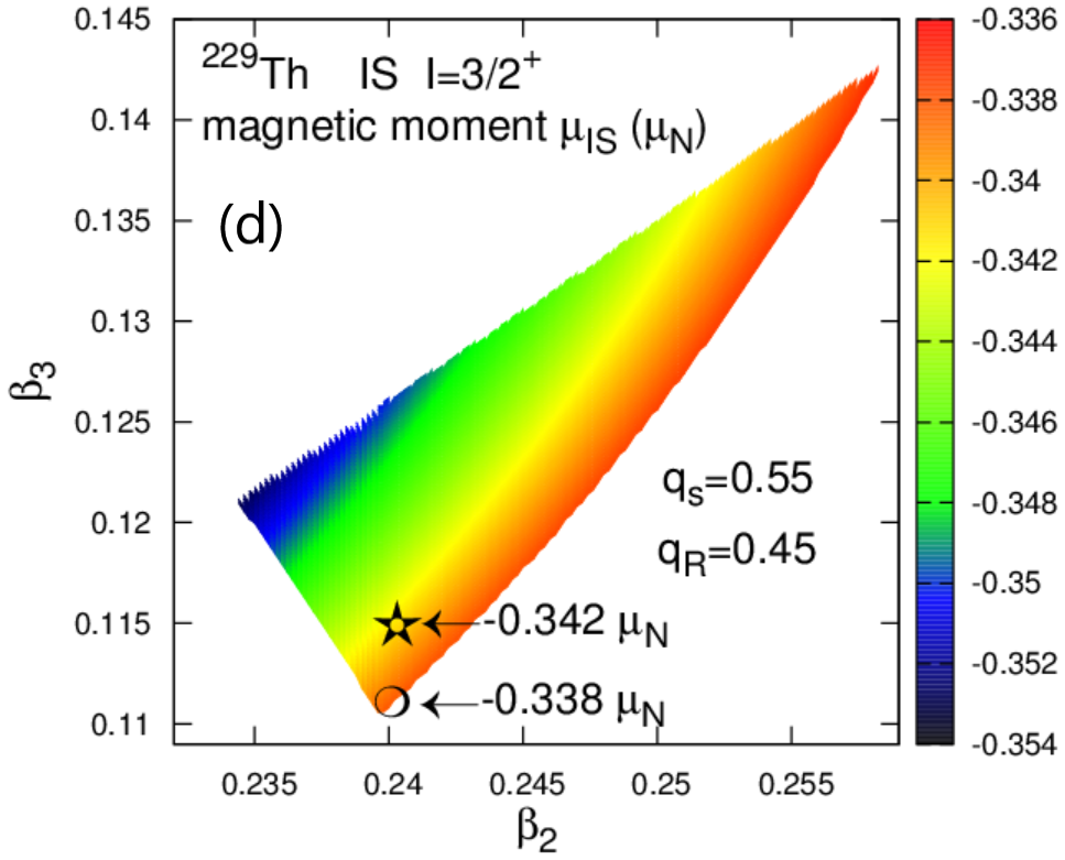
Figure 12: IS magnetic moment values obtained by the model fits on the model-defined QO deformation space grid at four different combinations of $q_{s}$ and $q_{R}$. The open star and the circle indicate the same sets of deformations as shown in Fig. 10.

The results obtained for the isomeric $B(M1;\,3/2^{+}_{\mbox{\scriptsize IS}}\rightarrow 5/2^{+}_{\mbox{\scriptsize GS}}$) and $B(E2;\,3/2^{+}_{\mbox{\scriptsize IS}}\rightarrow 5/2^{+}_{\mbox{\scriptsize GS}}$) transition rates are illustrated in Figs. 8 and 9, respectively, for the four sets of quenching factors. As in the energy analysis above, here we mark with an open star the value obtained by the model at the pair of QO deformations ($\beta_{2},\beta_{3}$)=($0.240,0.115$), adopted in Refs. Minkov and Pálffy (2017, 2019), for which the original model predictions for the transition rates and magnetic moments were made. Also, we examine the model predictions towards the line of $5/2^{+}$–$3/2^{+}$ orbitals degeneracy by considering in the graphs of ($q_{s},q_{R}$)=($0.55,0.45$) the pair of deformations ($\beta_{2},\beta_{3}$)=($0.240,0.111$) indicated by the open circle. Inspecting Fig. 8, first we observe that the overall behaviour of the $B(M1;\,3/2^{+}_{\mbox{\scriptsize IS}}\rightarrow 5/2^{+}_{\mbox{\scriptsize GS}}$) transition value shows an increase with the approaching of the degeneracy line. This is due to the circumstance that with the decreasing distance between both orbitals $5/2^{+}$ and $3/2^{+}$, the $K$-mixing effect generated by the matrix element in Eq. (5) sharply increases and this leads to the increase in the connecting transition rates. It should be noted, however, that in the model procedure this increase is counterbalanced by the adjustable parameter $A$ which drops accordingly thus preventing a deterioration of the model description due to the excessive mixing force. This will be discussed in more detail in the following (see Fig. 13 and related text below). Keeping in mind this clarification, we notice in Fig. 8(d) that while the quenching of the gyromagnetic factors leads to a reduction of $B(M1)_{\mbox{\scriptsize IS}}$ to 0.005 W.u. at ($\beta_{2},\beta_{3}$)=($0.240,0.115$) (an effect already addressed in Ref. Minkov and Pálffy (2019)), the shift of the deformation towards the degeneration line returns the value back to 0.007 W.u., i.e. in the original range of the prediction made in Ref. Minkov and Pálffy (2017).

A similar behaviour of the $B(E2;\,3/2^{+}_{\mbox{\scriptsize IS}}\rightarrow 5/2^{+}_{\mbox{\scriptsize GS}}$) transition rate in the model deformation space is observed in Fig. 9. We note that here all obtained $B(E2)_{\mbox{\scriptsize IS}}$ values exceed the previous prediction Minkov and Pálffy (2017) but stay in the range of the correction suggested in Ref. Minkov and Pálffy (2019).

III.5 Ground-state and isomer magnetic moments

The calculated GS magnetic moment $\mu_{\mbox{\scriptsize GS}}$ for the four sets of quenching factors ($q_{s},q_{R}$) is illustrated in Fig. 10. The overall model behaviour of this quantity is such that it decreases both with the attenuation of the gyromagnetic factors and with the approaching of the $5/2^{+}$–$3/2^{+}$ orbital-degeneracy line. We see that for ($\beta_{2},\beta_{3}$)=($0.240,0.115$) it drops to 0.45 $\mu_{N}$, while with the shift of the deformations to the point ($0.240,0.111$) it reaches the value of 0.43 $\mu_{N}$. The latter result is obviously due to the increasing Coriolis mixing which reduces the value of $\mu_{\mbox{\scriptsize GS}}$ as has been shown already in Ref. Minkov and Pálffy (2019). However, it appears that for model conditions considered physically reasonable, this is still not sufficient to reproduce the newer experimental value of 0.360(7) $\mu_{N}$ Safronova et al. (2013), although the model reproduces fairly well the earlier measured value of 0.46(4) $\mu_{N}$ Gerstenkorn et al. (1974).

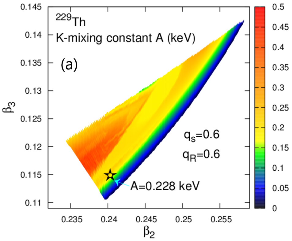
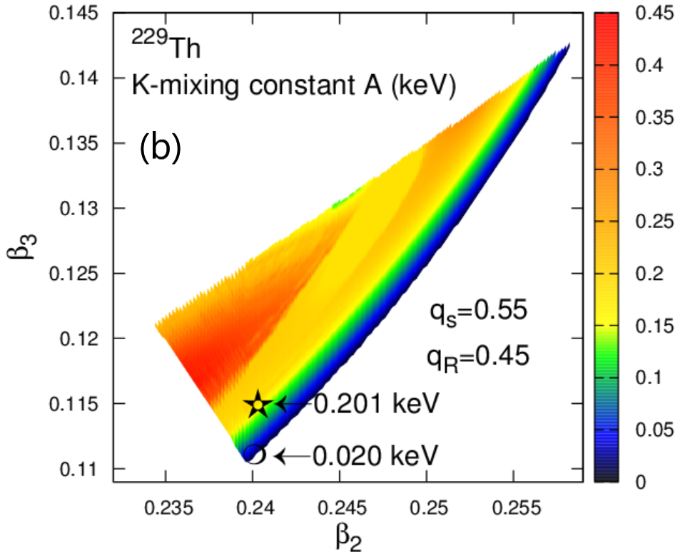
Figure 13: Values of the $K$-mixing constant $A$ obtained by the model fits on the model-defined QO deformation space grid at two different combinations of $q_{s}$ and $q_{R}$. The open star and the circle indicate the same sets of deformations as shown in Fig. 10.

It is instructive to check here also the “bare” values of $\mu_{\mbox{\scriptsize GS}}$, i.e. those obtained by the pure s.p. wave function without including the Coriolis mixing. Therefore, in Fig. 11 we show the analog of Fig. 10(a) (with $q_{s}=q_{R}=0.6$) in which $\mu_{\mbox{\scriptsize GS}}$ is calculated in the absence of Coriolis mixing with the $K$-mixing constant $A=0$. In this case Eq. (30) reduces to the terms in its first line with the second term involving the expression of Eq. (31). Here we first see that $\mu_{\mbox{\scriptsize GS}}$ appears with considerably larger values in the limits $\mu_{\mbox{\scriptsize GS}}$=0.55–0.60 $\mu_{N}$ which also show different behaviour in the DSM QO space compared with the Coriolis-mixing case. This result does not depend on the model-parameters fit and illustrates the genuine contribution of the QO deformation for the formation of the GS magnetic moment of ²²⁹Th. Comparing both plots we see that in the pure s.p. case without Coriolis mixing, the lowest $\mu_{\mbox{\scriptsize GS}}=0.55$ $\mu_{N}$ value appears in the left-upper vertex of the triangle model space, whereas in the Coriolis-mixing case the low values (lower than the pure s.p. ones), appear in the lower vertex of the space.

The above result leads us to the following conclusions. The Coriolis effect causes a decrease of the nuclear magnetic moment in the ²²⁹Th GS throughout the model deformation space. It plays a considerable role in our approach for fixing the GS magnetic moment through the overall model fits, although this is still not enough to reproduce the latest adopted experimental value. The appearance of essentially lower $\mu_{\mbox{\scriptsize GS}}$-values obtained through the adjusted $K$-mixing constant $A$ compared with the corresponding pure s.p. $\mu_{\mbox{\scriptsize GS}}$-values shows that the increase of the model-controlled Coriolis-mixing towards the $5/2^{+}$–$3/2^{+}$ orbitals-degeneracy line essentially determines the behaviour of the GS magnetic moment and dominates over the corresponding effect of changing QO deformation on the pure s.p. $\mu_{\mbox{\scriptsize GS}}$-values. This conclusion suggests that no considerably different result can be reached through further variation of deformations parameters in the DSM QO space.

Figure 12 shows the calculated IS magnetic moment $\mu_{\mbox{\scriptsize IS}}$ for the four sets of gyromagnetic quenching factors considered ($q_{s},q_{R}$). We note its relatively flat behaviour as a function of the QO deformation, with a slight increase towards the degeneracy line. Since $\mu_{\mbox{\scriptsize IS}}$ is practically not affected by the $K$-mixing effect, we may claim that this dependence can be considered as the bare effect of the changing structure of the s.p. wave functions along the deformation space. We see that in all plots of Fig. 12 the lowest value of $\mu_{\mbox{\scriptsize IS}}$ appears in the left upper corner of the model space similarly to the “bare” (s.p.) $\mu_{\mbox{\scriptsize GS}}$ case (Fig. 11). For example in the case of $q_{s}=q_{R}=0.6$, Fig. 12(a), the corresponding lowest value $\mu_{\mbox{\scriptsize IS}}$=$-$0.36 $\mu_{N}$ comes closer to the experimental result. However, the model fits have shown that the lower corner provides better predictions for $\mu_{\mbox{\scriptsize GS}}$, and we keep our attention on this region. Besides, for all considered quenching factors ($q_{s},q_{R}$), the theoretical $\mu_{\mbox{\scriptsize IS}}$ values appearing in Fig. 12 enter the error bars of the recent experimental value of $-$0.37(6) $\mu_{N}$ reported in Ref. Thielking et al. (2018); Müller et al. (2018).

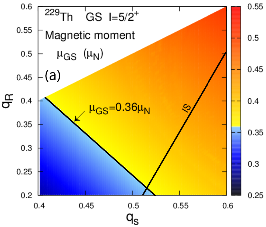
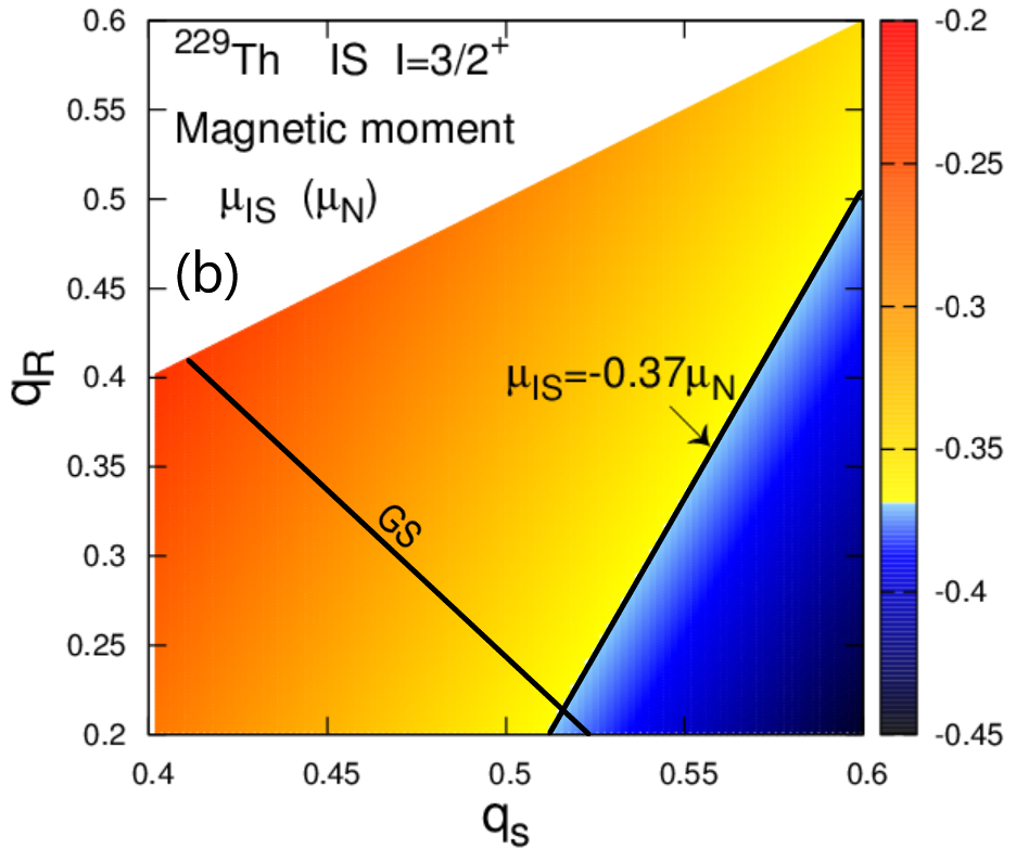
Figure 14: (a) GS and (b) IS magnetic moment values obtained by the model fits on a grid for the spin-gyromagnetic, $q_{s}$, and rotation-gyromagnetic, $q_{R}$, attenuation factors. The black lines show the values that would reproduce the corresponding GS and IS experimental values.

The results presented so far already reveal important details and relations characterizing the model mechanism upon which the ^229mTh isomer is formed and its spectroscopic properties develop. Obviously the proximity of the 5/2[633] and 3/2[631] s.p. orbitals plays a major role providing the overall condition for the appearance of a low-lying excitation. Now this is clearly quantified by all above plots. On the other hand, it is also clear that the appearance of the isomer can not be due only to the orbital quasidegeneracy. The reason is that at the distance of few eV the mixing between the two orbitals becomes very large and pushes all related observables in unphysical regions of magnitude. In this case the perturbation terms in the centrifugal part, Eq. (3), of the Hamiltonian as well as in the Coriolis perturbed wave function, Eq. (21), collapse in a singularity. The model prevents this situation mostly through the $K^{2}$ term and $K$-mixing constant $A$ in Eq. (3), which allow us to properly situate both GS and IS, i.e., to obtain the IS energy value as small as necessary, by keeping the 3/2[631]–5/2[633] orbital distance aside from the degeneracy line. In this respect one can say that the physically adequate QO deformations are slightly aside from this line.

The model mechanism feature described above can be seen by following the behaviour of the Coriolis mixing constant $A$ adjusted at each grid point in the deformation space. We investigate this in Fig. 13 for two sets of quenching factors, $(q_{s},q_{R})=(0.6,0.6)$ and $(0.55,0.45)$. The obtained values of $A$ range from zero to approximately 0.5 keV. Towards the degeneracy line, where the $K$-mixing matrix element in Eq. (5) connecting the two orbitals sharply increases as they approach each other, the adjustment algorithm strongly reduces the value of $A$. In this way the model “feels” the growing magnitude of the Coriolis mixing and tries to compensate its excessive effect on the considered observables through the parameter $A$ keeping them in physically meaningful ranges. Providing this balancing role of the parameter $A$ and having in mind all so far obtained model patterns for the spectroscopic observables in ²²⁹Th we can be rather confident in the consistency of the analysis made and the reliability of the QO deformation region outlined.

Finally, it is interesting to identify the degree of spin and collective gyromagnetic factor attenuations required to reproduce in the present model both experimental $\mu_{\mbox{\scriptsize GS}}$ and $\mu_{\mbox{\scriptsize IS}}$ values. This is shown in Fig. 14, where the values of each of these quantities obtained in the model fits at ($\beta_{2},\beta_{3}$)=($0.240,0.115$) are given [Fig. 14(a) for $\mu_{\mbox{\scriptsize GS}}$ and Fig. 14(b) for $\mu_{\mbox{\scriptsize IS}}$] as functions of the quenching factors $q_{s}$ and $q_{R}$. The black lines denote the pairs of ($q_{s},q_{R}$) values which provide the corresponding $\mu_{\mbox{\scriptsize GS}}$ and $\mu_{\mbox{\scriptsize IS}}$ experimental values. The crossing of both lines shows the point at which both magnetic moments are reproduced together. We see that this occurs at $q_{s}\approx 0.52$ and a rather low value of $q_{R}\approx 0.22$, which corresponds to a quite strong attenuation of the collective gyromagnetic factor. Because this quenching magnitude is hard to justify, we conclude that the agreement between the present theoretical model and the currently adopted experimental value of the GS magnetic moment remains an open issue.

IV Summary and conclusion

In this work we have thoroughly examined the physical conditions for the formation of the 8 eV isomer of ²²⁹Th according to the model mechanism suggested by our QO vibration-rotation core plus particle approach. First, we have determined the model deformation space encompassing the Woods-Saxon DSM quadrupole and octupole deformations which allow the appearance of the GS and IS with the experimentally adopted $K$-values and parities. We were able to clearly identify its borders constrained by the average parity of the isomer and the crossings of the 3/2[631] orbital on which the IS is built with the 5/2[633] orbital of the GS as well as with a 7/2[743] orbital. This space is rather limited and essentially constrains the QO deformation in the s.p. potential within the ranges $0.235\leq\beta_{2}\leq 0.255$ and $0.11\leq\beta_{3}\leq 0.14$. These results lead us to the important conclusion that the appearance of the $K^{\pi}=3/2^{+}$ IS through this mechanism is only possible in the presence of essentially nonzero octupole deformation in the s.p. potential.

Furthermore, we have examined the dependence of the overall DSM+CQOM model description on the QO deformations within the DSM model space. Our analysis of the CQOM fits made in Sec. III.2, including the CQOM potential-bottom semiaxes and dynamical deformations, showed that the collective CQOM conditions under which the ^229mTh isomer is formed consistently interrelate with the relevant conditions provided by the odd-nucleon degrees of freedom. Under these overall conditions we obtain for all of the considered observables, $B(M1;\,3/2^{+}_{\mbox{\scriptsize IS}}\rightarrow 5/2^{+}_{\mbox{\scriptsize GS}}$), $B(E2;\,3/2^{+}_{\mbox{\scriptsize IS}}\rightarrow 5/2^{+}_{\mbox{\scriptsize GS}}$), $\mu_{\mbox{\scriptsize GS}}$, $\mu_{\mbox{\scriptsize IS}}$ and $E(3/2^{+})_{IS}$ a smooth behaviour of the model predictions and descriptions compared with the results obtained for the fixed pair of Woods-Saxon DSM QO deformations considered in our previous works Minkov and Pálffy (2017, 2019), with the only peculiarity appearing close to the line of $5/2^{+}$–$3/2^{+}$ degeneracy where the mixing of both orbitals exceeds the perturbation theory limits. On the other hand the corresponding behaviour of the model energy RMS factors and Coriolis mixing constant shows that descriptions obtained with values of the above observables essentially deviating from those obtained in Minkov and Pálffy (2017, 2019) are of lower quality and/or violate the perturbation limit. For the remaining descriptions we have verified that in the limits of moderate deviations of the considered observables from the original values in Minkov and Pálffy (2017, 2019), the model is renormalizable, so that through a small variation of model parameters and on the expense of small deteriorations of the RMS factor, we can get very similar model predictions for the different pairs of QO deformations. Using this model feature as well as assuming possible stronger attenuation of the spin and collective gyromagnetic factors, we have outlined rather narrow limits of arbitrariness in which the model values of each of the above quantities can vary by keeping its reasonable physical meaning and predictability.

Our main conclusion is that within the obtained model deformation space the applied QO core plus particle approach provides a rather constrained prediction for the most important ²²⁹Th energy and electromagnetic characteristics related to the formation and manifestation of the 8 eV isomer. This allows us to generally reconfirm the predictions initially made in Ref. Minkov and Pálffy (2017, 2019) and to summarize them with a slight update: The $B(M1)$ IS transition remains in the limits 0.006-0.008 W.u. with an open possibility towards lower values such as 0.005 W.u.; the $B(E2)$ IS transition may be considered with slightly higher values between 30 and 50 W.u., compared with those in Ref. Minkov and Pálffy (2017); the GS magnetic moment allows a limited possibility for variation and remains with a model value around 0.50 $\mu_{N}$ possibly getting values as smaller as 0.43-0.48 $\mu_{N}$ under a stronger assumption for the gyromagnetic factors attenuation, thus covering the old experimental value of Ref Gerstenkorn et al. (1974), but still overestimating the newer one of Ref. Safronova et al. (2013); the theoretical IS magnetic moment firmly reproduces the recent experimental value within the uncertainty limits reported in Thielking et al. (2018); Müller et al. (2018) and this is obtained under all considered model conditions; and finally the model values for the isomer energy typically obtained around 1 keV and below suggest that with a small variation of parameters, and with the expense of a minor deterioration of the other energy levels, the model can easily reproduce the experimental value, although this is of little importance due to the overall limitation of the model accuracy in the energy-spectrum description.

We note that for all of the above quoted values the other model observables (energy levels and transition rates), for which experimental data are available, remain described within the accuracy limits reported in Ref. Minkov and Pálffy (2017). Thus our analysis suggests that within the above outlined limits of arbitrariness the model predictions could provide reliable estimates for the ^229mTh spectroscopic characteristics which could serve to the experiment in further efforts to observe and control the yet elusive radiative isomer transition.

Finally, the results obtained confirm the relevance of the model mechanism emphasizing on the role of the fine interplay between nuclear collective and intrinsic degrees of freedom as a plausible reason for the isomer formation. On this basis we conclude that the same dynamical mechanism may govern also in other nuclei the formation of excitations close to the border of atomic physics energy scale. Such states may exist being not yet observed due to experimental difficulties similar to those encountered in ^229mTh. As in this work we give a detailed prescription about the examination and constraining of the physical conditions under which such a phenomenon may emerge, it appears promising to extend the study to other nuclei in the same or other mass regions. In this aspect the close neighbour ²³¹Th as well as the ^235mU isomer would be natural candidates for such a study. This could be a subject of future work.

References

- Beck et al. (2007) B. R. Beck, J. A. Becker, P. Beiersdorfer, G. V. Brown, K. J. Moody, J. B. Wilhelmy, F. S. Porter, C. A. Kilbourne, and R. L. Kelley, Phys. Rev. Lett. 98, 142501 (2007), URL https://link.aps.org/doi/10.1103/PhysRevLett.98.142501.
- Bec (2009) Improved Value for the Energy Splitting of the Ground-State Doublet in the Nucleus , vol. LLNL-PROC-415170 (Varenna, Italy, 2009).
- Seiferle et al. (2019) B. Seiferle et al., Nature (London) 573, 243 (2019).
- Yamaguchi et al. (2019) A. Yamaguchi et al., Phys. Rev. Lett. 123, 222501 (2019).
- Browne and Tuli (2014) E. Browne and J. K. Tuli, Nuclear Data Sheets 122, 205 (2014).
- E. Peik and Chr. Tamm (2003) E. Peik and Chr. Tamm, Europhys. Lett. 61, 181 (2003), URL https://doi.org/10.1209/epl/i2003-00210-x.
- Peik and Okhapkin (2015) E. Peik and M. Okhapkin, Comptes Rendus Physique 16, 516 (2015), ISSN 1631-0705, the measurement of time / La mesure du temps, URL http://www.sciencedirect.com/science/article/pii/S1631070515000213.
- Campbell et al. (2012) C. J. Campbell, A. G. Radnaev, A. Kuzmich, V. A. Dzuba, V. V. Flambaum, and A. Derevianko, Phys. Rev. Lett. 108, 120802 (2012), URL https://link.aps.org/doi/10.1103/PhysRevLett.108.120802.
- Flambaum (2006) V. V. Flambaum, Phys. Rev. Lett. 97, 092502 (2006), URL https://link.aps.org/doi/10.1103/PhysRevLett.97.092502.
- Berengut et al. (2009) J. C. Berengut, V. A. Dzuba, V. V. Flambaum, and S. G. Porsev, Phys. Rev. Lett. 102, 210801 (2009), URL https://link.aps.org/doi/10.1103/PhysRevLett.102.210801.
- Rellergert et al. (2010) W. G. Rellergert, D. DeMille, R. R. Greco, M. P. Hehlen, J. R. Torgerson, and E. R. Hudson, Phys. Rev. Lett. 104, 200802 (2010), URL https://link.aps.org/doi/10.1103/PhysRevLett.104.200802.
- Fadeev et al. (2020) P. Fadeev, J. C. Berengut, and V. V. Flambaum, Phys. Rev. A 102, 052833 (2020), URL https://journals.aps.org/pra/abstract/10.1103/PhysRevA.102.052833.
- Tkalya (2011) E. V. Tkalya, Phys. Rev. Lett. 106, 162501 (2011), URL https://link.aps.org/doi/10.1103/PhysRevLett.106.162501.
- von der Wense et al. (2016) L. von der Wense, B. Seiferle, M. Laatiaoui, J. B. Neumayr, H.-J. Maier, H.-F. Wirth, C. Mokry, J. Runke, K. Eberhardt, C. E. Düllmann, et al., Nature 533, 47 (2016), ISSN 0028-0836, article, URL http://dx.doi.org/10.1038/nature17669.
- Seiferle et al. (2017) B. Seiferle, L. von der Wense, and P. G. Thirolf, Phys. Rev. Lett. 118, 042501 (2017), URL https://link.aps.org/doi/10.1103/PhysRevLett.118.042501.
- Thielking et al. (2018) J. Thielking, M. V. Okhapkin, P. Glowacki, D. M. Meier, L. von der Wense, B. Seiferle, C. E. Düllmann, P. G. Thirolf, and P. Peik, Nature (London) 556, 321 (2018).
- Müller et al. (2018) R. A. Müller, A. V. Maiorova, S. Fritzsche, A. V. Volotka, R. Beerwerth, P. Glowacki, J. Thielking, D.-M. Meier, M. Okhapkin, E. Peik, et al., Phys. Rev. A 98, 020503 (2018), URL https://link.aps.org/doi/10.1103/PhysRevA.98.020503.
- Sikorsky et al. (2020) T. Sikorsky, J. Geist, D. Hengstler, S. Kempf, L. Gastaldo, C. Enss, C. Mokry, J. Runke, C. E. Düllmann, P. Wobrauschek, et al., Phys. Rev. Lett. 125, 142503 (2020), URL https://journals.aps.org/prl/abstract/10.1103/PhysRevLett.125.142503.
- Nilsson and Ragnarsson (1995) S. G. Nilsson and I. Ragnarsson, Shapes and Shells in Nuclear Structure (Cambridge University Press, Cambridge, 1995).
- Gulda et al. (2002) K. Gulda, W. Kurcewicz, A. Aas, M. Borge, D. Burke, B. Fogelberg, I. Grant, E. Hagebø, N. Kaffrell, J. Kvasil, et al., Nuclear Physics A 703, 45 (2002), ISSN 0375-9474, URL http://www.sciencedirect.com/science/article/pii/S0375947401014567.
- Ruchowska et al. (2006) E. Ruchowska, W. A. Płóciennik, J. Żylicz, H. Mach, J. Kvasil, A. Algora, N. Amzal, T. Bäck, M. G. Borge, R. Boutami, et al., Phys. Rev. C 73, 044326 (2006).
- G. (1976) S. V. G., Theory of Complex Nuclei (Pergamon Press, Oxford, 1976).
- Dykhne and Tkalya (1998) A. M. Dykhne and E. V. Tkalya, JETP Lett. 67, 251 (1998).
- Tkalya et al. (2015) E. V. Tkalya, C. Schneider, J. Jeet, and E. R. Hudson, Phys. Rev. C 92, 054324 (2015), URL https://link.aps.org/doi/10.1103/PhysRevC.92.054324.
- Alaga et al. (1955) G. Alaga, K. Alder, A. Bohr, and B. Mottelson, Kgl. Danske Videnskab. Selskab Mat.-fys. Medd. 29 (No. 9), 1 (1955).
- Nilsson (1955) S. G. Nilsson, Kgl. Danske Videnskab. Selskab Mat.-fys. Medd. 29 (No. 16), 1 (1955).
- Minkov and Pálffy (2017) N. Minkov and A. Pálffy, Phys. Rev. Lett. 118, 212501 (2017).
- Minkov et al. (2006) N. Minkov, P. Yotov, S. Drenska, W. Scheid, D. Bonatsos, D. Lenis, and D. Petrellis, Phys. Rev. C 73, 044315 (2006), URL https://link.aps.org/doi/10.1103/PhysRevC.73.044315.
- Minkov et al. (2007) N. Minkov, S. Drenska, P. Yotov, S. Lalkovski, D. Bonatsos, and W. Scheid, Phys. Rev. C 76, 034324 (2007), URL https://link.aps.org/doi/10.1103/PhysRevC.76.034324.
- Minkov et al. (2012) N. Minkov, S. Drenska, M. Strecker, W. Scheid, and H. Lenske, Phys. Rev. C 85, 034306 (2012), URL https://link.aps.org/doi/10.1103/PhysRevC.85.034306.
- Minkov et al. (2013) N. Minkov, S. Drenska, K. Drumev, M. Strecker, H. Lenske, and W. Scheid, Phys. Rev. C 88, 064310 (2013), URL https://link.aps.org/doi/10.1103/PhysRevC.88.064310.
- Cwiok et al. (1987) S. Cwiok, J. Dudek, W. Nazarewicz, J. Skalski, and T. Werner, Computer Physics Communications 46, 379 (1987), ISSN 0010-4655, URL http://www.sciencedirect.com/science/article/pii/0010465587900932.
- Ring and Schuck (1980) P. Ring and P. Schuck, The Nuclear Many-Body Problem (Springer Verlag, New York, 1980).
- Jeet et al. (2015) J. Jeet, C. Schneider, S. T. Sullivan, W. G. Rellergert, S. Mirzadeh, A. Cassanho, H. P. Jenssen, E. V. Tkalya, and E. R. Hudson, Phys. Rev. Lett. 114, 253001 (2015), URL https://link.aps.org/doi/10.1103/PhysRevLett.114.253001.
- Yamaguchi et al. (2015) A. Yamaguchi, M. Kolbe, H. Kaser, T. Reichel, A. Gottwald, and E. Peik, New Journal of Physics 17, 053053 (2015), URL http://stacks.iop.org/1367-2630/17/i=5/a=053053.
- von der Wense L. (2018) von der Wense L., On the direct detection of 229mTh (Springer Thesis Series, Springer International Publishing, 2018).
- Minkov and Pálffy (2019) N. Minkov and A. Pálffy, Phys. Rev. Lett. 122, 162502 (2019).
- Safronova et al. (2013) M. S. Safronova, U. I. Safronova, A. G. Radnaev, C. J. Campbell, and A. Kuzmich, Phys. Rev. A 88, 060501(R) (2013), URL https://link.aps.org/doi/10.1103/PhysRevA.88.060501.
- Gerstenkorn et al. (1974) S. Gerstenkorn, P. Luc, J. Verges, D. W. Englekemeir, J. E. Gindler, and F. S. Tomkins, J. Phys. (Paris) 35, 483 (1974).
- Chasman et al. (1977) R. R. Chasman, I. Ahmad, A. M. Friedman, and J. R. Erskine, Rev. Mod. Phys. 49, 833 (1977), URL https://link.aps.org/doi/10.1103/RevModPhys.49.833.
- Walker and Minkov (2010) P. Walker and N. Minkov, Physics Letters B 694, 119 (2010), ISSN 0370-2693, URL http://www.sciencedirect.com/science/article/pii/S0370269310011378.
- Minkov (2013) N. Minkov, Physica Scripta T154, 014017 (2013), URL http://stacks.iop.org/1402-4896/2013/i=T154/a=014017.
- Minkov et al. (2010) N. Minkov, S. Drenska, M. Strecker, and W. Scheid, Journal of Physics G: Nuclear and Particle Physics 37, 025103 (2010), URL http://stacks.iop.org/0954-3899/37/i=2/a=025103.
- Mottelson (1960) B. R. Mottelson, Selected Topics in the Theory of Collective Phenomena in Nuclei (Int. School of Phys., Varenna, Nordita Publ. no. 78, 1960).
- Way (1939) K. Way, Phys. Rev. 55, 963 (1939), URL https://link.aps.org/doi/10.1103/PhysRev.55.963.
- Bodenstedt (1962) E. Bodenstedt, Fortsch. Physik 10, 321 (1962).
- Eisenberg and Greiner (1970) J. Eisenberg and W. Greiner, Nuclear Theory: Nuclear Models, Vol. I (North-Holland, Amsterdam, 1970).
- Nilsson and Prior (1961) S. G. Nilsson and O. Prior, Kgl. Danske Videnskab. Selskab Mat.-fys. Medd. 32 (No. 16), 1 (1961).
- Prior et al. (1968) O. Prior, F. Boehm, and S. G. Nilsson, Nucl. Phys. A 110, 257 (1968).
- Greiner (1965) W. Greiner, Phys. Rev. Lett. 14, 599 (1965), URL https://link.aps.org/doi/10.1103/PhysRevLett.14.599.
- Raman et al. (2001) S. Raman, C. W. Nestor, Jr., and P. Tikkanen, At. Data Nucl. Data Tables 78, 1 (2001), ISSN 0092-640X, URL http://www.sciencedirect.com/science/article/pii/S0092640X01908587.
- Nomura et al. (2014) K. Nomura, D. Vretenar, T. Nikšić, and B.-N. Lu, Phys. Rev. C 89, 024312 (2014), URL https://link.aps.org/doi/10.1103/PhysRevC.89.024312.
- Nikšić et al. (2008) T. Nikšić, D. Vretenar, and P. Ring, Phys. Rev. C 78, 034318 (2008), URL https://link.aps.org/doi/10.1103/PhysRevC.78.034318.