Sub-grid scale characterization and asymptotic behavior of multi-dimensional upwind schemes for the vorticity transport equations

Abstract

We study the sub-grid scale characteristics of a vorticity-transport-based approach for large-eddy simulations. In particular, we consider a multi-dimensional upwind scheme for the vorticity transport equations and establish its properties in the under-resolved regime. The asymptotic behavior of key turbulence statistics of velocity gradients, vorticity, and invariants is studied in detail. Modified equation analysis indicates that dissipation can be controlled locally via non-linear limiting of the gradient employed for the vorticity reconstruction on the cell face such that low numerical diffusion is obtained in well-resolved regimes and high numerical diffusion is realized in under-resolved regions. The enstrophy budget highlights the remarkable ability of the truncation terms to mimic the true sub-grid scale dissipation and diffusion. The modified equation also reveals diffusive terms that are similar to several commonly employed sub-grid scale models including tensor-gradient and hyper-viscosity models. Investigations on several canonical turbulence flow cases show that large-scale features are adequately represented and remain consistent in terms of spectral energy over a range of grid resolutions. Numerical dissipation in under-resolved simulations is consistent and can be characterized by diffusion terms discovered in the modified equation analysis. A minimum state of scale separation necessary to obtain asymptotic behavior is characterized using metrics such as effective Reynolds number and effective grid spacing. Temporally-evolving jet simulations, characterized by large-scale vortical structures, demonstrate that high Reynolds number vortex-dominated flows are captured when criteria is met and necessitate diffusive non-linear limiting of vorticity reconstruction be employed to realize accuracy in under-resolved simulations.

I Introduction

Coherent structures are prominent in a wide range of turbulent flows including jets Yule (1978); Akselvoll and Moin (1996), wakes Foti et al. (2016, 2018), and atmospheric flows Guala et al. (2011); Fang and Porté-Agel (2015). The critical characteristics of such flows are defined to a large extent by the dynamics of dominant coherent structures, pointing to large-eddy simulation (LES) as an ideal candidate model. In classical LES, a scale-separation is performed typically via a low-pass filter, and a sub-grid scale model is imposed to represent the impact of the unresolved scales on the resolved scales. In practice, the sub-grid scale model provides a pathway for energy to dissipate from the resolved scales because physical dissipation mechanisms (i.e., viscous dissipation at the Kolmogorov scale) are unresolved. However, the accuracy of LES at high Reynolds numbers is significantly influenced by discretization errors Kravchenko and Moin (1997); Chow and Moin (2003); Freitag and Klein (2006); Toosi and Larsson (2020), as these errors can be of a similar magnitude as the sub-grid scale model in practical scenarios. Despite this fundamental obstacle, functional Smagorinsky (1963); Germano et al. (1991); Bardina et al. (1980); Lilly (1992); Clark et al. (1979); Bou-Zeid et al. (2005); Yu et al. (2017); Chapelier et al. (2018) and structural Schneider et al. (2005); Ouvrard et al. (2010); Parish and Duraisamy (2017a, b); Geurts (1997); Zhou et al. (2018); Kraichnan (1970) LES sub-grid scale models are actively developed and applied to practical flows with varying degrees of success.
An alternate view eschews the explicit modeling of sub-grid scales and instead focuses on tailoring numerical dissipation in the underlying discretization errors. Monotone integrated LES (MILES), first proposed by Boris et al. Boris et al. (1992), utilizes functional reconstruction of the convective fluxes in a monotonicity-preserving finite volume scheme to integrate the effects of the sub-grid scale on the resolved scale. Results from similar numerical methods also were observed by Youngs Youngs (1991) around the same time. A more broadly-defined methodology, referred to as implicit LES (ILES), requires a careful consideration of discretization errors. Typically, ILES employs a certain class of numerical methods, most notably monotonic upwind finite volume methods such as piece-wise parabolic Gathmann et al. (1993), MPDATA Smolarkiewicz and Margolin (1998), total variation diminishing Thornber et al. (2007) and flux-corrected transport Wachtor et al. (2013), which have implicit dissipation mechanisms Boris et al. (1992); Margolin and Rider (2002, 2005). In practice, ILES methods are employed on inertially dominated (e.g., high Reynolds number) dynamics and regularize the under-resolved scales similar to the way in which shock-capturing, non-oscillating finite volume schemes use weak solutions and satisfy the entropy condition.

Thorough analysis of the schemes reveals the errors are often similar in form to certain sub-grid scale models Margolin et al. (2006). However, the form of the discretization errors does not necessarily has to be similar to a sub-grid scale model provided the dissipation acts on the high wavenumber range. Drikakis et al Drikakis et al. (2009) characterized the effect of numerical resolution on the dissipation into two categories: a) When the solution is well-resolved and an adequate distinction between the start of the inertial range and the dissipation scales exists, the numerical dissipation should not influence the large scales, and the eddies interacting with the largest scales should be reasonably resolved. The separation of scales should not depend on the form of the dissipation; b) The second category involves inadequate numerical resolution, which is often confronted in engineering applications. Given an inadequate separation between the large and dissipative scales, the numerical scheme should be designed to mimic the impact of dissipation on the large scales. Many ILES solution fall under this category including isotropic turbulence Thornber et al. (2007); Zhou et al. (2014); Hickel et al. (2006), geophysical flows Smolarkiewicz and Margolin (1998); Margolin et al. (1999), jets Fureby and Grinstein (2002); Boris et al. (1992); Grinstein and Fureby (2007) and channel flows Grinstein and Fureby (2007).
In many vortex-dominated problems, especially those in which the vorticity distribution is compact Hussain (1986); Papamoschou and Lele (1993); Duraisamy and Lele (2008) the vorticity-velocity formulation of the Navier–Stokes equations has the potential to be advantageous in comparison to the pressure-velocity form Koumoutsakos and Leonard (1995); Foti and Duraisamy (2018). Despite the use of a wide array of Eulerian Brown and Line (2005); Whitehouse and Boschitsch (2014), Lagrangian Koumoutsakos (2005); Winckelmans et al. (1996) and mixed numerical implementations Cottet (1990); Ould-Salihi et al. (2001) of the vorticity transport equations, modeling of unresolved dynamics remains an outstanding issue. Further, while ILES has been prominently utilized in the context of the velocity-pressure formulation, the authors are not aware of literature investigating implicit sub-grid scale characterizations for schemes using the vorticity-velocity formulation. The goal of this work is to explore how tailored numerical schemes of vorticity-velocity formulation are suitable and can be characterized for ILES.

The vorticity-velocity formulation of the incompressible vorticity transport equations (VTE), obtained by applying the curl operator to the momentum equations. While there is an increase to six (three vorticity and three velocity) variables compared to four (three velocity and one pressure) variables in three dimensions, the formulation is advantageous in flows with compact vorticity distributions typical of vortex-dominated flow, as the potential flow regions do not need to be part of the computational domain. In Eulerian methods, accurate boundary conditions can be developed Rennich and Lele (1997); Duraisamy and Lele (2008); Koumoutsakos and Leonard (1995), allowing for efficient simulations in a compact domain. Further, the Poisson equation for pressure, normally a stiff equation, is replaced by the kinematic velocity-vorticity relationship.

Numerical schemes Zhao and He (2011); Stone et al. (2010); Koumoutsakos (2005) using the Lagrangian description of the flow field have seen considerable success and have applied the LES methodology through development of vorticity sub-grid scale models Winckelmans et al. (1996); Mansfield et al. (1998). Both Refs. Winckelmans et al. (1996); Mansfield et al. (1998) introduced eddy-viscosity type sub-grid scale models for the vorticity-velocity formulation using the Lagrangian description. However, Lagrangian frameworks are not optimal for a wide range of turbulent flows. Furthermore, a priori tests of forced homogeneous, isotropic turbulence in Ref. Mansfield et al. (1998) reveal that both vorticity convection and vortex stretching contribute to sub-grid scale dissipation, but the dissipation due to vortex stretching is inadequately captured by the sub-grid scale model. On the other hand, relatively few Eulerian vorticity numerical schemes have been developed Brown and Line (2005); Meitz and Fasel (2000); Davies and Carpenter (2001). Recently developed upwind finite volume methods for the VTE Whitehouse and Boschitsch (2014); Parish et al. (2016); Foti and Duraisamy (2018) have been shown to efficiently capture and preserve vortical structures with relatively coarse resolution (a few grid cells spanning vortex cores). Consistent integration of both the vorticity convection and vortex stretching terms is a prominent feature of schemes in Refs. Parish et al. (2016); Foti and Duraisamy (2018). While these schemes fit into the philosophy of ILES, an understanding of their sub-grid scale behavior has not been established in the context of turbulent flows.
Margolin et al. Margolin et al. (2006) used modified equation analysis to examine leading order diffusive and dispersive error terms. Based on a Taylor series representation, the modified equation is the effective partial differential equation satisfied by the numerical method. Their work specifically addresses finite volume approaches, and thus volume-averaged filtering. The leading terms in the modified equation are used to elucidate the dissipative effects on the large resolved scales. As the numerical resolution of the scheme increases, the dissipation should focus on a narrowing range of high wavenumbers and not impact the large scales. Several studies Zhou et al. (2014); Thornber et al. (2007) emphasized the calculation of an effective viscosity or Reynolds number for a given grid resolution with resolved features. Since the filter and dissipation are based on the grid resolution, it is imperative to understand whether there is a sufficient separation of resolved and dissipation scales. A minimum state of scale separation is necessary to reproduce high Reynolds numbers flows with asymptotic turbulence statistics Zhou et al. (2014); Chamorro et al. (2012). In this work, we will examine the utility of a finite volume scheme for the VTE Parish et al. (2016); Foti and Duraisamy (2018), characterizes its ILES properties and provide a methodology to estimate effective Reynolds numbers. This particular formulation has a number of features pertinent for ILES: Consistent integration of vorticity convection and vortex stretching terms, promoting stability and accuracy and the ability to represent and preserve sharp gradients. Rigorous characterization of the sub-grid scale behavior in canonical turbulent flows enables the use of VTE-based schemes in complex vortex-dominated turbulent flows such as in rotorcraft and wind turbine wakes.
We begin the study by introducing the governing and filtered equations in Sec. II. We provide a description of the numerical scheme and analyze the implicit sub-grid scale model in Secs. III and IV, respectively. We detail the results of numerical experimentation of canonical turbulence flows in Sec. V. Finally, we conclude our work and provide details for future studies in Sec. VI.

II Governing and Filtered Equations

We employ the vorticity-velocity formulation of the Navier-Stokes equations obtained by applying the curl operator to the incompressible mass and momentum equations. In compact index notation, the unsteady, three-dimensional incompressible VTE are as follows ($i,j=1,2,3$):

$$\frac{\partial\omega_{i}}{\partial t}+\frac{\partial}{\partial x_{j}}\left(u_{j}\omega_{i}-u_{i}\omega_{j}\right)=f_{i}+\frac{1}{Re}\frac{\partial^{2}\omega_{i}}{\partial x_{j}\partial x_{j}},$$ (1)

where $u_{i}$ is the velocity and $\omega_{i}=\epsilon_{ijk}\partial u_{k}/\partial x_{j}$ is the vorticity, the curl of the velocity where $\epsilon_{ijk}$ is the Levi-Civita tensor. $f_{i}$ is the curl of the body force and $Re=\frac{UL}{\nu}$ is the Reynolds number defined by a characteristic velocity scale $U$, characteristic length $L$, and kinematic viscosity $\nu$. The inviscid fluxes in Eqn. (1) can be rewritten in quasi-linear form as follows:

$$\frac{\partial\omega_{i}}{\partial t}+A_{1}\frac{\partial}{\partial x_{1}}\omega_{i}+A_{2}\frac{\partial}{\partial x_{2}}\omega_{i}+A_{3}\frac{\partial}{\partial x_{3}}\omega_{i}=0,$$ (2)

where the eigenvalues of matrix $A_{1}$ are $\lambda_{1}=\{0,u_{1},u_{1}\}$, $A_{2}$ are $\lambda_{2}=\{u_{2},0,u_{2}\}$, $A_{3}$ are $\lambda_{3}=\{u_{3},u_{3},0\}$. The eigenvector matrices $R_{i}$ for $A_{i}$ are

$$R_{1}=\begin{bmatrix}u_{1}&0&0\\ u_{2}&1&0\\ u_{3}&0&1\\ \end{bmatrix},\>R_{2}=\begin{bmatrix}1&u_{1}&0\\ 0&u_{2}&0\\ 0&u_{3}&1\\ \end{bmatrix},\>R_{3}=\begin{bmatrix}1&0&u_{1}\\ 0&1&u_{2}\\ 0&0&u_{3}\\ \end{bmatrix}.$$ (3)

These equations are degenerate in a hyperbolic sense. As an example, if any component of $u$ equals zero, then the eigenvectors are linearly dependent. This presents difficulties for construction of stable upwind schemes. This is similar to ideal magneto-hydrodynamics, for which Godunov Godunov (1972) suggested the addition of a symmetrizing term. Following this idea and Ref. Parish et al. (2016), an additional term is included to stabilize the governing equations. The equations are thus modified in the form

$$\frac{\partial\omega_{i}}{\partial t}+\frac{\partial}{\partial x_{j}}\left(u_{j}\omega_{i}-u_{i}\omega_{j}\right)+u_{i}\frac{\partial\omega_{j}}{\partial x_{j}}=f_{i}+\frac{1}{Re}\frac{\partial^{2}\omega_{i}}{\partial x_{j}\partial x_{j}},$$ (4)

Included with the VTE due to the incompressible assumption, is the solenoidality of both the velocity and vorticity fields:

$$\frac{\partial u_{i}}{\partial x_{i}}=\frac{\partial\omega_{i}}{\partial x_{i}}=0.$$ (5)

We refer to Eqn. (4) as the modified VTE because the final term on the LHS is an additional term, which is proportional to the divergence of vorticity. Analytically, the term is zero (Eqn. (5)), but numerically, this stabilizes the hyperbolic system of equations. The modification in Eqn. (4) stabilizes the equations with eigenvalues $\lambda_{i}=\{u_{i},u_{i},u_{i}\}$ and the eigenvectors of the canonical basis vector for $\mathbb{R}^{3}$ Parish et al. (2016). A similar modification is used in the magneto-hydrodynamic equations to enforce a divergence-free magnetic field Powell (1997), however, in our context we employ the modification for numerical stability.
The vorticity-velocity formulation in three dimensions has six unknowns. While the three vorticity variables are obtained through the VTE, a supplemental equation is needed to obtain the velocity induced by the vorticity. The vorticity-velocity relationship is written in the form of a Poisson equation as follows:

$$\frac{\partial^{2}u_{i}}{\partial x_{j}\partial x_{j}}=-\epsilon_{ijk}\frac{\partial\omega_{k}}{\partial x_{j}}.$$ (6)

II.1 The Filtered vorticity transport equations

By spatial filtering the VTE in Eqn. (4), we obtain the following filtered VTE:

$$\frac{\partial\widetilde{\omega}_{i}}{\partial t}+\frac{\partial}{\partial x_{j}}\left(\widetilde{u}_{j}\widetilde{\omega}_{i}-\widetilde{\omega}_{j}\widetilde{u}_{i}\right)+\widetilde{u}_{i}\frac{\partial\widetilde{\omega}_{j}}{\partial x_{j}}=\widetilde{f}_{i}+\frac{1}{Re}\frac{\partial^{2}\widetilde{\omega}_{i}}{\partial x_{j}\partial x_{j}}-\frac{\partial\tau_{ij}}{\partial x_{j}},$$ (7)

where $\widetilde{\cdot}$ indicates the spatial filtering or a resolved quantity and the $\tau_{ij}$ is the sub-grid scale (SGS) vorticity stress due to the filtering operation. We note that filtering is not performed through an explicit filter function, and we assume that the filtering operation and the derivatives commute. The grid cell of the mesh at a size $\Delta$ is an implicit physical-space sharp cut-off filter where the velocity and vorticity fluctuations can only be resolved at a size greater than $\Delta$. The SGS torque, the divergence of the SGS vorticity stress, which accounts for the unresolved velocity and vorticity fluctuations, is defined as

$$\frac{\partial\tau_{ij}}{\partial x_{j}}=\frac{\partial}{\partial x_{j}}\left[\left(\widetilde{u_{j}\omega_{i}}-\widetilde{u}_{j}\widetilde{\omega}_{i}\right)-\left(\widetilde{u_{i}\omega_{j}}-\widetilde{u}_{i}\widetilde{\omega}_{j}\right)\right]+\left[\widetilde{u_{i}\frac{\partial\omega_{j}}{\partial x_{j}}}-\widetilde{u}_{i}\frac{\partial\widetilde{\omega}_{j}}{\partial x_{j}}\right].$$ (8)

The SGS torque term is composed of three different terms: 1.) the vorticity transport by unresolved velocity fluctuations, 2.) the unresolved vortex stretching, and 3.) the unresolved contributions for the vorticity divergence modification in Eqn. (4). Unlike previous LES schemes for the VTE Winckelmans et al. (1996); Mansfield et al. (1998) where there is not an additional vorticity divergence term, the SGS vorticity stress tensor is not purely anti-symmetric. Here, we attempt to rearrange the SGS terms. The first two terms in Eqn. (8) can be combined into a single anti-symmetric tensor as follows:

$$\left(\tau_{ij}\right)_{a}=\left(\widetilde{u_{j}\omega_{i}}-\widetilde{u}_{j}\widetilde{\omega}_{i}\right)-\left(\widetilde{u_{i}\omega_{j}}-\widetilde{u}_{i}\widetilde{\omega}_{j}\right).$$ (9)

However, the third term introduced through the vorticity divergence modification cannot be readily decomposed into an SGS vorticity stress tensor and as such it remains a separate term of the SGS torque:

$$\left(\frac{\partial\tau_{ij}}{\partial x_{j}}\right)_{d}=\widetilde{u_{i}\frac{\partial\omega_{j}}{\partial x_{j}}}-\widetilde{u}_{i}\frac{\partial\widetilde{\omega}_{j}}{\partial x_{j}}.$$ (10)

However, through manipulation, this term can be rewritten as follows:

$$\frac{\partial\left(\tau_{ij}\right)_{m}}{\partial x_{j}}=\left(\frac{\partial\widetilde{\omega_{j}u_{i}}}{\partial x_{j}}-\frac{\partial\widetilde{\omega_{j}}\widetilde{u_{i}}}{\partial x_{j}}\right)-\left(\widetilde{\omega_{j}s_{ij}}-\widetilde{\omega_{j}}\widetilde{s_{ij}}\right),$$ (11)

where $s_{ij}=\frac{1}{2}(\partial_{j}u_{i}+\partial_{i}u_{j})$ is the strain rate. We can obtain another two portions of the SGS terms. The first divergence modification contains terms that are similar to the third and fourth terms in Eqn. (9):

$$\left(\tau_{ij}\right)_{d}=\widetilde{u_{i}\omega_{j}}-\widetilde{u}_{i}\widetilde{\omega}_{j}$$ (12)

While the other term contains the strain rate:

$$\frac{\partial\left(\tau_{ij}\right)_{s}}{\partial x_{j}}=-\left(\widetilde{\omega_{j}s_{ij}}-\widetilde{\omega_{j}}\widetilde{s_{ij}}\right).$$ (13)

The practical purpose of these terms in the LES methodology is to provide a pathway of energy transfer between the resolved scales to the unresolved (sub-grid) scales, which is enabled by ensuring additional dissipation.

III Multi-dimensional upwind finite volume

We employ a multi-dimensional upwind finite volume approach to numerically integrate the VTE. This approach, within the philosophy of the ILES, is similar to Lax-Wendroff-like schemes where upwind differences are corrected by second-order transverse flux corrections to produce a solution that is second-order accurate in space and time. Our multi-dimensional scheme is solved in a series of dimensional sweeps. The total flux across a cell face in each direction is the sum of several fluxes accounting for both normal and transverse directional fluxes. A simplified two-dimensional flux is demonstrated in Fig. 1. The updated vorticity is computed as shown (for clarity vectors are shown in bold and $\tilde{\cdot}$ removed from all variables):

$$\bm{\omega}^{n+1}_{i,j,k}=\bm{\omega}^{n}_{i,j,k} -\frac{\Delta t}{\Delta_{x_{1}}}\left[\left((\bm{F}_{1}^{l})^{n}_{i+\frac{1}{2},j,k}-(\bm{F}_{1}^{r})^{n}_{i-\frac{1}{2},j,k}\right)-\left((\bm{G}_{1})^{n}_{i+\frac{1}{2},j,k}-(\bm{G}_{1})^{n}_{i-\frac{1}{2},j,k}\right)\right]$$ (14)

$$-\frac{\Delta t}{\Delta_{x_{2}}}\left[\left((\bm{F}_{2}^{l})^{n}_{i,j+\frac{1}{2},k}-(\bm{F}_{2}^{r})^{n}_{i,j-\frac{1}{2},k}\right)-\left((\bm{G}_{2})^{n}_{i,j+\frac{1}{2},k}-(\bm{G}_{2})^{n}_{i,j-\frac{1}{2},k}\right)\right]$$

$$-\frac{\Delta t}{\Delta_{x_{3}}}\left[\left((\bm{F}_{3}^{l})^{n}_{i,j,k+\frac{1}{2}}-(\bm{F}_{3}^{r})^{n}_{i,j,k-\frac{1}{2}}\right)-\left((\bm{G}_{3})^{n}_{i,j,k+\frac{1}{2}}-(\bm{G}_{3})^{n}_{i,j,k-\frac{1}{2}}\right)\right],$$

where $n$ is the time iteration and $i,j,k$ are the indices of the grid cell centers in three directions. The flux functions $\bm{F}^{l},\bm{F}^{r}$ are normal directional (with respect to the cell faces) fluxes and are obtained by solving a generalized Riemann problem developed for the VTE Parish et al. (2016). In order to account for the fluxes traveling oblique to the cell faces while simultaneously increasing numerical stability and accuracy, transverse fluxes are included. The transverse directional flux functions $\bm{G}$ are computed using the flux-based wave propagation approach Foti and Duraisamy (2018). All flux functions are stored at the cell faces. Note that both left and right normal flux functions $\bm{F}_{i}^{l}$ and $\bm{F}_{i}^{r}$, respectively, are stored at each cell face, while a single transverse flux function $\bm{G}_{i}$ is stored at each cell face.

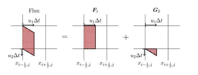
Figure 1: Sketch of multi-dimensional scheme using both normal $\bm{F}_{1}$ and transverse $\bm{G}_{2}$ fluxes .

First, we detail the normal directional fluxes $\bm{F}_{i}^{l},\bm{F}_{i}^{r}$, which are determined by allowing the vorticity to be discontinuous at the cell face. The sharp discontinuity-capturing scheme can be beneficial for simulating turbulence that is dominated by large coherent structures. In flows such as these, regions that are dominated by coherent structures can be efficiently captured by compact vorticity variables. On the other hand, in under-resolved turbulence regions, the scheme adds additional numerical dissipation (more discussion on this in section IV).
The solution to the generalized Riemann problem for vorticity, which is allowed to be discontinuous across the cell face, begins by reconstructing the vorticity stored at the cell center on the cell face. For simplicity, we will focus on the Riemann problem at cell face $(i+1/2,j,k)$ and translated to $x_{1}=0$. The initial condition for the Riemann problem is

$$\bm{\omega}_{0}(x_{1},0)=\left\{\begin{array}[]{@{}ll@{}}\bm{\omega}^{L}+\left(x_{1}+\frac{1}{2}\Delta_{x}\right)\bm{s}^{L},&\text{if}\ x_{1}<0\\ \bm{\omega}^{R}+\left(x_{1}-\frac{1}{2}\Delta_{x}\right)\bm{s}^{R},&\text{if}\ x_{1}>0\\ \end{array}\right.,$$ (15)

where $(\cdot)^{L}$ at ${i,j,k}$, $(\cdot)^{R}$ is at ${i+1,j,k}$, $\Delta_{x}$ is the cell size, $\bm{s}$ is the slope of the vorticity. Achieving second order accuracy via slope reconstruction is beneficial in maximizing the separation of scales for ILES. In areas of smooth vorticity a second-order accurate central difference can be used, however, as with most second-order accurate discontinuity-capturing schemes, an appropriate slope needs to be used, and a limiter is employed. A limiter reduces the slope calculation to a first-order accurate difference and effectively adds numerical diffusion.
Integrating the vorticity transport equations, equation (4), with the vorticity reconstruction, equation (15), over the space $\left[-\frac{1}{2}\Delta_{x},\frac{1}{2}\Delta_{x}\right]\times[0,\Delta t]$, where $\Delta t$ is the time step, a left moving flux $\bm{F}^{l}_{1}$ and right moving flux $\bm{F}^{r}_{1}$ are obtained at the cell face as follows ($\bm{F}^{r,l}_{2}$ and $\bm{F}^{r,l}_{3}$ follow similarly):

$$\bm{F}^{l}_{1}=\left\{\begin{array}[]{@{}ll@{}}u_{1}\hat{\bm{\omega}}^{L}-\bm{u}\hat{\omega}_{1}^{L}+\frac{1}{2}\bm{u}s^{L}_{1}\Delta_{x},&\text{if}\ u_{1}\geq 0\\ u_{1}\hat{\bm{\omega}}^{R}-\bm{u}\hat{\omega}_{1}^{R}+\frac{1}{2}\bm{u}s^{R}_{1}\Delta_{x}+\bm{u}\left[\frac{1}{2}\left(s^{L}_{1}-s^{R}_{1}\right)u_{1}\Delta t+\left(\tilde{\omega}^{L}_{1}-\tilde{\omega}^{R}_{1}\right)\right],&\text{if}\ u_{1}<0,\end{array}\right.$$ (16)

$$\bm{F}^{r}_{1}=\left\{\begin{array}[]{@{}ll@{}}u_{1}\hat{\bm{\omega}}^{L}-\bm{u}\hat{\omega}_{1}^{L}-\frac{1}{2}\bm{u}s^{R}_{1}\Delta_{x}-\bm{u}\left[\frac{1}{2}\left(s^{L}_{1}-s^{R}_{1}\right)u_{1}\Delta t+\left(\tilde{\omega}^{L}_{1}-\tilde{\omega}^{R}_{1}\right)\right],&\text{if}\ u_{1}\geq 0\\ u_{1}\hat{\bm{\omega}}^{R}-\bm{u}\hat{\omega}_{1}^{R}-\frac{1}{2}\bm{u}s^{R}_{1}\Delta_{x},&\text{if}\ u_{1}<0,\end{array}\right.$$ (17)

where for conciseness, additional vorticity reconstruction variables are created:

$$\hat{\bm{\omega}}^{L}=\bm{\omega}^{L}+\frac{1}{2}\bm{s}^{L}\left(\Delta_{x}-u_{1}\Delta t\right),\ \ \hat{\bm{\omega}}^{R}=\bm{\omega}^{R}-\frac{1}{2}\bm{s}^{R}\left(\Delta_{x}+u_{1}\Delta t\right),\ \ \tilde{\omega}^{L}_{1}=\omega^{L}_{1}+\frac{1}{2}s^{L}_{1}\Delta_{x},\ \ \tilde{\omega}^{R}_{1}=\omega^{R}_{1}-\frac{1}{2}s^{R}_{1}\Delta_{x}.$$

Next, we detail the computation of the transverse fluxes. In this scheme we pursue a flux-based wave decomposition introduced in Ref. Bale et al. (2003), where the flux difference, $F^{l}-F^{r}$, is rewritten as a linear combination of eigenvectors. This choice is motivated because the solution to the generalized Riemann problem is known, is linearly independent in each direction, and can be used directly without costly manipulations. In this implementation, the fluxes, $\bm{F}_{1}^{l}$ and $\bm{F}_{1}^{r}$, only need to be computed once (per time-step), and the transverse fluxes are evaluated with that solution. The flux difference is decomposed into f-waves $\mathcal{Z}^{p}$, the flux wave, as follows:

$$\bm{F}^{l}-\bm{F}^{r}=\sum_{p=0}^{m}\beta^{p}r^{p}\equiv\sum_{p=1}^{m}\mathcal{Z}^{p},$$ (18)

and

$$\bm{\beta}=R^{-1}\left(\bm{F}^{l}-\bm{F}^{r}\right),$$ (19)

where the eigenmatrix $R$ is simply the identity matrix Foti and Duraisamy (2018).
From Eqn. (19) and the eigensystem, we obtained a simple relationship for the f-waves $\mathcal{Z}^{p}=\bm{F}^{l}-\bm{F}^{r}$ exactly. The relationship allows for the multi-dimensional wave propagation corrections to be implemented equivalently to a three-dimensional advection equation described in Ref. LeVeque (1996) if the f-waves are normalized by the eigenvalues $\lambda_{i}$.
In a multi-dimensional problem, the fluxes propagate in the transverse $x_{2}$- and $x_{3}$-direction depending on the wave speed given by the eigenvalues of the Jacobian, which are exactly the velocities $u_{i}$ at the cell face. The transverse fluxes are implemented by using the f-waves and transverse velocity at the grid cell $(i,j,k)$ and updating the transverse fluxes in surrounding cells. The most important transverse fluxes are the two-dimensional fluxes given by the following:

$$(\bm{G}_{2})^{n}_{I,J-\frac{1}{2},k} =-\frac{1}{2}\frac{\Delta t}{\Delta x_{1}}u_{2}\mathcal{Z}_{1},$$ (20)

$$(\bm{G}_{3})^{n}_{I,j,K-\frac{1}{2}} =-\frac{1}{2}\frac{\Delta t}{\Delta x_{1}}u_{3}\mathcal{Z}_{1},$$

where $n$ is the time step iteration and the indices for the grid cell influenced by the transverse flux are given by

$$I=\left\{\begin{array}[]{@{}ll@{}}i,&\text{if}\>u_{1}>0\\ i-1,&\text{if}\>u_{1}<0\end{array}\right.,\>\>J=\left\{\begin{array}[]{@{}ll@{}}j+1,&\text{if}\>u_{2}>0\\ j,&\text{if}\>u_{2}<0\end{array}\right.,\>\>K=\left\{\begin{array}[]{@{}ll@{}}k+1,&\text{if}\>u_{3}>0\\ k,&\text{if}\>u_{3}<0\end{array}\right..$$

Additional transverse fluxes are employed, which account for three-dimensional fluxes as well as higher-order corrections. For a detailed implementation see Foti and Duraisamy Foti and Duraisamy (2018).

IV Modified equation analysis

In the following, we present the modified equation analysis (MEA) for the multi-dimensional generalized Riemann problem-based upwind finite volume scheme. MEA analysis was first proposed in Ref. Hirt (1968) and subsequently used to characterize the unresolved scales for ILES Margolin and Rider (2002); Margolin et al. (2006). The intuition is that in certain classes of numerical methods, the effects of the unresolved scales can be represented by the truncation error of the discretization. This analysis must be carefully exploited when considering high Reynolds number turbulent flows discretized with upwind finite volume schemes. Slope limiting with a multi-dimensional scheme yields a complex, nonlinear scheme. In particular, the dissipation is proportional to the multi-dimensional interfacial wave jumps. It must also be recognized that in under-resolved flows, the leading order terms may not necessarily be the best approximator of the truncation terms.
Due to the complexity of including the exact form of the slope limiter employed in the vorticity reconstruction in the scheme, two limiting cases of the modified equation are analyzed: 1.) the vorticity at the cell interface is smooth and a second-order central difference can be employed, and 2.) the vorticity at the cell interface is discontinuous and a limiter switches the slope to a first-order upwind difference.

The procedure to develop the modified equation begins with expanding the scheme with Taylor series expansions Hirt (1968); Margolin and Rider (2005). For example, the scheme in Eqn. (14) contains the following, which can be substituted with a series expansion:

$$\frac{\omega_{i}^{n+1}-\omega_{i}^{n}}{\Delta t}=\frac{\partial\omega_{i}}{\partial t}+\frac{\Delta t}{2}\frac{\partial^{2}\omega_{i}}{\partial t^{2}}+\frac{\Delta t^{2}}{6}\frac{\partial^{3}\omega_{i}}{\partial t^{3}}+\mathcal{O}(\Delta t^{3}),$$ (21)

where $n$ is the vorticity at $t$ and $n+1$ is the vorticity at $t+\Delta t$. Similarly, all terms in the flux functions in Eqns. (16), (17), (20) can be substituted with Taylor series expansions in terms of vorticity as a function of time $t$ or space $\bm{x}$. The accumulation of all expansions in the scheme can be manipulated to include terms in Eqn. (4) as follows:

$$\frac{\partial\omega_{i}}{\partial t}+\frac{\partial}{\partial x_{j}}\left(u_{j}\omega_{i}-u_{i}\omega_{j}\right)+u_{i}\frac{\partial\omega_{j}}{\partial x_{j}}=\nu\frac{\partial^{2}\omega_{i}}{\partial x_{j}\partial x_{j}}+T_{ij},$$ (22)

where $T_{ij}$ is the term that includes all second-order accurate and higher terms from the series expansions not included in the VTE. The remainder is manipulated to substitute temporal derivative terms with spatial terms using the governing equations. As such, the remainder $T_{ij}$ is a complex function that contains many high order spatial derivatives of the vorticity and velocity. In the philosophy of ILES, the leading order terms in the expansion term $T_{ij}$ are related to the SGS vorticity stress $R_{ij}$ due to truncation as follow:

$$T_{ij}=\frac{\partial}{\partial x_{j}}R_{ij}+\mathcal{O}(\Delta_{x}^{3}).$$ (23)

$T_{ij}$ acts as an implicit sub-grid scale model, which is completely dependent on resolved variables. Note that there is a distinction between the SGS vorticity stress $R_{ij}$ due to truncation and theoretical SGS vorticity stress $\tau_{ij}$ due to filtering. In what follows we demonstrate that by changing the form of the slope employed in the vorticity reconstruction on the cell face, the modified equation can be tailored.
First, we examine terms that remain after the VTE is subtracted from the Taylor series expansion of the scheme in smooth regions and a second-order accurate central difference is employed, i.e. $s^{l}_{1}=1/(2\Delta_{x})\left(\omega(x+\Delta_{x})-\omega(x-\Delta_{x})\right)$. In turbulent flows in which we are interested, a smooth spatial region of vorticity often corresponds to a resolved (or nearly resolved) region dominated by a large-scale coherent vortical structure.

In the modified equation analysis, the lowest order remaining terms are second-order accurate terms in space and are considered to have the largest influence on the scheme. Moreover, these terms can be collected to implicitly provide a model for the SGS torque. Eqn. (24) shows the second-order accurate terms that make up the implicit SGS torque. For clarity in presentation, only the $x_{1}$ and $x_{2}$ directions are shown ($j=1,2$); however, the third $x_{3}$ direction follows the same form:

$$\frac{\partial R_{1j}}{\partial x_{j}} =\Delta_{1}^{2}\left(\frac{1}{12}u_{1}\frac{\partial^{3}\omega_{1}}{\partial x_{1}^{3}}-\frac{1}{4}u_{1}\frac{\partial^{3}\omega_{1}}{\partial x_{1}^{3}}-\frac{1}{8}\frac{\partial^{2}u_{1}}{\partial x_{1}^{2}}\frac{\partial\omega_{1}}{\partial x_{1}}+\frac{1}{12}u_{2}\frac{\partial^{3}\omega_{1}}{\partial x_{2}^{3}}-\frac{1}{4}u_{1}\frac{\partial^{3}\omega_{2}}{\partial x_{1}^{3}}-\frac{1}{8}\frac{\partial^{2}u_{2}}{\partial x_{2}^{2}}\frac{\partial\omega_{1}}{\partial x_{2}}\right),$$ (24)

$$\frac{\partial R_{2j}}{\partial x_{j}} =\Delta_{2}^{2}\left(\frac{1}{12}u_{1}\frac{\partial^{3}\omega_{2}}{\partial x_{1}^{3}}-\frac{1}{4}u_{2}\frac{\partial^{3}\omega_{1}}{\partial x_{2}^{3}}-\frac{1}{8}\frac{\partial^{2}u_{1}}{\partial x_{1}^{2}}\frac{\partial\omega_{2}}{\partial x_{1}}+\frac{1}{12}u_{2}\frac{\partial^{3}\omega_{2}}{\partial x_{2}^{3}}-\frac{1}{4}u_{2}\frac{\partial^{3}\omega_{2}}{\partial x_{2}^{3}}-\frac{1}{8}\frac{\partial^{2}u_{2}}{\partial x_{2}^{2}}\frac{\partial\omega_{2}}{\partial x_{2}}\right),$$

where $\Delta_{i}$ is the grid cell size in the $i$th direction. All terms are dispersive (containing odd-ordered derivatives of vorticity) in nature indicating that in smooth regions where a second-order central difference is used, there are no second-order accurate implicit diffusive terms (even-ordered derivatives of vorticity), which can act as numerical routes for implicit SGS dissipation. We take a closer look at the diagonal terms ($\partial_{1}R_{11}$ and $\partial_{2}R_{22}$) of the SGS torque to obtain some insight into the effects of the modification of the vorticity transport equations and the effect of the anti-symmetric and non-symmetric SGS terms (due to Eqn. (9) and Eqn. (10), respectively).
By rewriting terms in Eqn. (24) that are associated with the diagonal terms of $R_{ij}$, an anti-symmetric part of the SGS torque associated with Eqn. (9), $\partial_{j}R^{a}_{ij}$, can be formed and shown to be equal to zero in the following:

$$\frac{\partial R^{a}_{11}}{\partial x_{1}} =\frac{1}{12}\Delta_{x}^{2}u_{1}\frac{\partial^{3}\omega_{1}}{\partial x_{1}^{3}}-\frac{1}{12}\Delta_{x}^{2}u_{1}\frac{\partial^{3}\omega_{1}}{\partial x_{1}^{3}}=0,$$ (25)

$$\frac{\partial R^{a}_{22}}{\partial x_{2}} =\frac{1}{12}\Delta_{x}^{2}u_{2}\frac{\partial^{3}\omega_{2}}{\partial x_{2}^{3}}-\frac{1}{12}\Delta_{x}^{2}u_{2}\frac{\partial^{3}\omega_{2}}{\partial x_{2}^{3}}=0.$$

The remaining leading order terms can collected into the following:

$$\frac{\partial R^{d}_{11}}{\partial x_{1}}=-\frac{1}{6}\Delta_{2}^{2}u_{1}\frac{\partial^{3}\omega_{1}}{\partial x_{1}^{3}}-\frac{1}{8}\Delta_{1}^{2}\frac{\partial^{2}u_{1}}{\partial x_{1}^{2}}\frac{\partial\omega_{1}}{\partial x_{1}},$$ (26)

$$\frac{\partial R^{d}_{22}}{\partial x_{2}}=-\frac{1}{6}\Delta_{1}^{2}u_{2}\frac{\partial^{3}\omega_{2}}{\partial x_{2}^{3}}-\frac{1}{8}\Delta_{2}^{2}\frac{\partial^{2}u_{2}}{\partial x_{2}^{2}}\frac{\partial\omega_{2}}{\partial x_{2}},$$

where $\partial_{j}R^{d}_{ij}$ is due to the modification term added to the vorticity transport equation. Terms associated with the off-diagonals of $R_{ij}$ contain dispersive terms. This modified equation of the scheme near a smooth vorticity field shows that there is a limiting case that can be used to reduce the amount of numerical dissipation added by the numerical method, which can control the sub-grid scale dissipation and energy transfer.
The next limiting case employs a limiter to reduce the order of the slope in regions in which vorticity gradients may be very large. In numerical simulations of turbulence, large gradients and discontinuities arise in under-resolved regions of the flow where gradients caused by eddies the size of the grid cell or larger cannot be smoothed by smaller scale eddies that are physically present in the flow but are not numerically captured. Towards this end, a forward/backward difference is employed. For example, the slope of the vorticity is calculated as $s^{l}_{1}=1/\Delta_{x}\left(\omega(x_{1})-\omega(x_{1}-\Delta_{x})\right)$. These eddies transfer energy in a turbulent flow, and the reduction in order of the slope essentially introduces diffusion into the solution in order to maintain non-oscillatory behavior. The lowest-order terms remaining from the modified equation are shown in the following (again we limit the result to two dimensions for clarity but the $x_{3}$-direction has the same form):

$$\frac{\partial R_{1j}}{\partial x_{j}}= \frac{\Delta_{1}}{2}u_{1}\frac{\partial^{2}\omega_{1}}{\partial x_{1}^{2}}+\Delta_{1}^{2}\left(-\frac{1}{8}\frac{\partial^{2}u_{1}}{\partial x_{1}^{2}}\frac{\partial\omega_{1}}{\partial x_{1}}-\frac{1}{6}u_{1}\frac{\partial^{3}\omega_{1}}{\partial x_{1}^{3}}\right)+$$ (27)

$$\frac{\Delta_{1}}{2}u_{2}\frac{\partial^{2}\omega_{1}}{\partial x_{2}^{2}}+\Delta_{1}^{2}\left(-\frac{1}{8}\frac{\partial^{2}u_{2}}{\partial x_{2}^{2}}\frac{\partial\omega_{1}}{\partial x_{2}}+\frac{1}{4}\frac{\partial u_{2}}{\partial x_{2}}\frac{\partial^{2}\omega_{1}}{\partial x_{2}^{2}}-\frac{1}{4}\frac{\partial u_{1}}{\partial x_{1}}\frac{\partial^{2}\omega_{2}}{\partial x_{1}^{2}}+\frac{1}{3}u_{2}\frac{\partial^{3}\omega_{1}}{\partial x_{2}^{3}}-\frac{1}{2}u_{1}\frac{\partial^{3}\omega_{2}}{\partial x_{1}^{3}}\right),$$

$$\frac{\partial R_{2j}}{\partial x_{j}}= \frac{\Delta_{2}}{2}u_{1}\frac{\partial^{2}\omega_{2}}{\partial x_{1}^{2}}+\Delta_{2}^{2}\left(-\frac{1}{8}\frac{\partial^{2}u_{1}}{\partial x_{1}^{2}}\frac{\partial\omega_{2}}{\partial x_{1}}+\frac{1}{4}\frac{\partial u_{1}}{\partial x_{1}}\frac{\partial^{2}\omega_{2}}{\partial x_{1}^{2}}-\frac{1}{4}\frac{\partial u_{2}}{\partial x_{2}}\frac{\partial^{2}\omega_{1}}{\partial x_{2}^{2}}+\frac{1}{3}u_{1}\frac{\partial^{3}\omega_{2}}{\partial x_{1}^{3}}-\frac{1}{2}u_{2}\frac{\partial^{3}\omega_{1}}{\partial x_{2}^{3}}\right)+$$ (28)

$$\frac{\Delta_{2}}{2}u_{2}\frac{\partial^{2}\omega_{2}}{\partial x_{2}^{2}}+\Delta_{2}^{2}\left(-\frac{1}{8}\frac{\partial^{2}u_{2}}{\partial x_{2}^{2}}\frac{\partial\omega_{2}}{\partial x_{2}}-\frac{1}{6}u_{2}\frac{\partial^{3}\omega_{2}}{\partial x_{2}^{3}}\right),$$

which include a single first-order accurate in space term and several second-order accurate terms. We can readily see that this case includes both diffusive and dispersive terms for vorticity. This indicates that limiting the slope of the vorticity is necessary to add diffusive terms to include dissipation to solve turbulent flows through an ILES. As with the first limiting case, a few of the terms in Eqn. (27) can be rewritten to show a zero diagonal of an anti-symmetric portion of the SGS torque in the following:

$$\frac{\partial R^{a}_{11}}{\partial x_{1}}=\Delta_{1}^{2}\left(\frac{1}{4}\frac{\partial u_{1}}{\partial x_{1}}\frac{\partial^{2}\omega_{1}}{\partial x_{1}^{2}}-\frac{1}{4}\frac{\partial u_{1}}{\partial x_{1}}\frac{\partial^{2}\omega_{1}}{\partial x_{1}^{2}}+\frac{1}{3}u_{1}\frac{\partial^{3}\omega_{1}}{\partial x_{1}^{3}}-\frac{1}{3}u_{1}\frac{\partial^{3}\omega_{1}}{\partial x_{1}^{3}}\right)=0.$$ (29)

Similarly, terms can be rearranged in $\partial_{2}R^{a}_{22}=0$ and $\partial_{3}R^{a}_{33}=0$. The rest of the terms in the diagonals are accumulated in the part of the SGS torque corresponding to the introduction of the vorticity divergence term modification, which includes a first-order accurate diffusive term.
The analysis reveals that each component in the SGS vorticity stress tensor $R_{ij}$ contains diffusive terms. In the following we select terms from Eqn. (27) to explore how the diffusion is present in the SGS vorticity stress tensor and its similarity to well-known SGS models. We emphasize that similarities to explicit SGS models are employed to just enhance our understanding of the ILES dissipation. In complex turbulent flows, the process of limiting the slope and multi-dimensionality can affect the actual leading terms of the modified equation such that they may not precisely mimic the action of explicit SGS models. We show that three separate diffusive SGS vorticity stress mechanisms are present in the modified equation and can be summed as follows:

$$R_{ij}=R^{g}_{ij}+R^{h}_{ij}+R^{t}_{ij}.$$ (30)

The first term is constructed as follows:

$$\frac{\partial R^{g}_{12}}{\partial x_{2}}=-\frac{1}{8}\Delta_{2}^{2}\frac{\partial^{2}u_{2}}{\partial x_{2}^{2}}\frac{\partial\omega_{1}}{\partial x_{2}}+\frac{1}{4}\Delta_{2}^{2}\frac{\partial u_{2}}{\partial x_{2}}\frac{\partial^{2}\omega_{1}}{\partial x_{2}^{2}},$$ (31)

We can manipulate the terms by introducing another dispersion term and integrating the SGS torque to obtain a single form for the off-diagonal elements in the SGS vorticity stress tensor, which can be written in index notion as follows:

$$R^{g}_{ij}=\frac{1}{4}\Delta^{2}\frac{\partial u_{j}}{\partial x_{k}}\frac{\partial\omega_{i}}{\partial x_{k}},$$ (32)

where $\Delta$ is the grid spacing in the $i$th direction. The form of the Eqn. (32) can be readily seen as a term similar to tensor-gradient models Clark et al. (1979); Borue and Orszag (1998); Vreman et al. (1996) for the sub-grid scale. These models have been shown to be not overly dissipative and are often paired with an eddy viscosity model Vreman et al. (1996); Borue and Orszag (1998). They also provide both dissipation and backscatter, an important aspect of turbulence, which is not possible in eddy viscosity-type models. However, when employed alone, the tensor-gradient model can be unstable Vreman et al. (1996).
An alternate form for the numerical dissipation can be explored with another group of dispersive and diffusive terms as shown in the following:

$$\frac{\partial R^{h}_{12}}{\partial x_{2}}=-\frac{1}{2}\Delta_{2}^{2}u_{2}\frac{\partial^{3}\omega_{1}}{\partial x_{2}^{3}}-\frac{1}{4}\Delta_{2}^{2}\frac{\partial u_{1}}{\partial x_{2}}\frac{\partial^{2}\omega_{1}}{\partial x_{2}^{2}},$$ (33)

where these terms again can be manipulated and integrated. The second numerical dissipation term for the SGS vorticity stress has the form :

$$R^{h}_{ij}=-\frac{1}{4}\Delta^{2}u_{j}\frac{\partial^{2}\omega_{i}}{\partial x_{k}\partial x_{k}}.$$ (34)

This term has the form that is similar to hyper-viscosity models Winckelmans et al. (1996); Cerutti et al. (2000), which have the form of $(-1)^{n+1}\nabla^{2n}\bm{u}$, where $n>1$. Ref. Cerutti et al. (2000) used the hyper-viscosity model for the SGS stress tensor with $\nabla^{2}\widetilde{s}_{ij}$, which was added to a standard Smagorinsky model and motivated by SGS dissipation of enstrophy. Hyper-viscosity models with increasing $n$ have less effect on dissipation and ‘bottleneck’ effects shown on the turbulence spectra Lamorgese et al. (2005). However, paired with the tensor-gradient model, it may provide less dissipation than is observed with standard mixed models.
With these two terms, all of the diffusive terms in the modified equation and SGS torque are accounted except for the single first-order diffusive term, which appears in both the diagonal and non-diagonal elements of the SGS vorticity stress tensor. This term can be integrated to show another form of the numerical dissipation:

$$R^{t}_{ij}=\frac{1}{2}\Delta u_{j}\frac{\partial\omega_{i}}{\partial x_{j}}.$$ (35)

These terms show that in the limit of a slope reconstruction with a first-order slope, there are several modes for additional numerical diffusion that can be used to increase the energy transfer from the resolved scales to the sub-grid scales and add dissipation.
The two limiting cases for the present scheme show that the dissipation of the scheme can be controlled using well-designed limiters for specific flows. The present scheme is developed to conserve coherent vortical structures in flows. When regions of the flow field are dominated by large coherent structures, which are not subject to the inertial range energy transfer determined by the SGS stresses, the vorticity tends to be smooth and less implicit dissipation is included. However, in regions of small-scale vortical structures where the flow field is under-resolved and discontinuities in the vorticity are present, the dissipation needs to be increased to account for the energy transfer to the sub-grid scales. This formulation provides a plausible framework to simulate large-scale features of turbulent flows without providing dissipation at all flow scales, a common problem for Smagorinsky-like explicit methods.

V Numerical Experimentation

In this section, we discuss results obtained through numerical experimentation of several canonical flows of turbulence in a periodic box. We investigate a Taylor-Green vortex in Sec. V.1, forced isotropic turbulence in Sec. V.2, and a temporally evolving jet in Sec. V.3. All simulations employ the multi-dimensional wave propagation approach described above.

V.1 Taylor-Green vortex

The Taylor-Green vortex is a well-studied flow field Frisch (1995); Brachet (1991); Brachet et al. (1983), which encompasses large structures, transition, and decaying turbulence, and is used to assess the ability of the scheme to capture the complexities of vortex stretching and breakdown using under-resolved grids Zhou et al. (2014); Drikakis et al. (2007); Grinstein et al. (2011). The test case is used to demonstrate how the present scheme can be employed to emulate the dominant sub-grid scales, most importantly dissipation, from the initial conditions of large coherent structures through a transition to turbulence at high Re. The initial velocity flow field for the Taylor-Green vortex is given by

$$u_{1}(x_{1},x_{2},x_{3}) =u_{0}\cos(kx_{1})\sin(kx_{2})\cos(kx_{3})$$

$$u_{2}(x_{1},x_{2},x_{3}) =-u_{0}\sin(kx_{1})\cos(kx_{2})\cos(kx_{3})$$ (36)

$$u_{3}(x_{1},x_{2},x_{3}) =0$$

where $u_{0}=1$ is the velocity scale and $k_{0}=1$ is the length scale of the flow field. Using these scales, the $\textrm{Re}=u_{0}/\nu k_{0}=1/\nu$, where $\nu$ is the dynamic viscosity specified for each simulations. Simulations are designed in a periodic cube with length $2\pi$ with a uniform grid. We start by exploring how well the scheme captures the pertinent physics at $\textrm{Re}=1600$ with a non-dissipative second-order central difference (referred to as no-limiter) and a high dissipative limiter, the minmod limiter. The first limiter is directly related with the results from the modified equation in section IV. On the other hand, the modified equation for the first-order backward slope detailed in section IV is only similar to the minmod limiter because the minmod limiter chooses between first-order backward and forward differences and removes slopes where the backward and forward differences have opposite slopes.
Figure 2 shows the energy spectra of simulations at several grid resolutions ($N=64,128$ and $256$) at two time instances $tu_{0}k_{0}=5$, during the transition to turbulence as the large-scale structures are breaking down, and $tu_{0}k_{0}=10$, near the maximum dissipation. Additionally, a spectral method solver Parish and Duraisamy (2017a) is employed to provide direct numerical simulation (DNS) comparisons. The DNS employs 256 spectral modes to fully resolve the flow. In Fig. 2(a), the low wavenumber region of the energy spectra in all simulations is able to be captured accurately compared the DNS results from the spectral method regardless of the slope limiter employed. The decline in energy in the spectrum for each simulation corresponds to the grid resolution where the lowest resolution begins to fall off at lowest wavenumbers. This is expected for the under-resolved simulations. The highest resolution case, while using the same number of degrees of freedom as the DNS, approaches the DNS solution but has slightly less energy in inertial range modes. Test cases that employ the minmod limiter have lower energy in modes starting near a wavenumber $k/k_{0}=10$ compared to the no-limiter limiter. It becomes noticeable in the lower resolution test cases at lower wavenumbers, however, they all occur in the inertial range. This is due to the dissipative nature of the minmod limiter, which allows for more implicit dissipation especially in modes that have a wavenumber comparable to the inverse size of the grid cell, $1/\Delta_{x}$. Figure 2(b) shows similar behavior for the energy spectra; however, the lowest grid resolution cases show an increased energy at low wavenumbers. This can be attributed to the evolution of the flow at this grid resolution because the number of necessary modes needed to provide an acceptable solution are higher than the number of modes resolved.

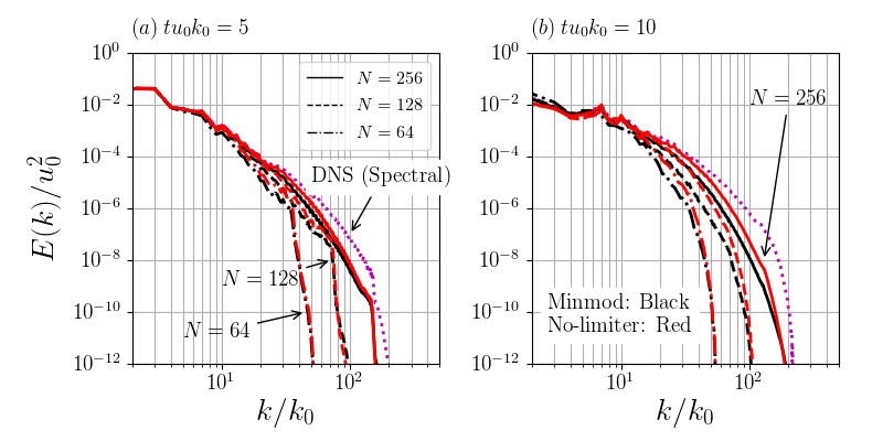
Figure 2: Energy spectra $E(k)$ of simulations at several under-resolved grid resolutions at $\mathrm{Re}=1600$ at (a) $tu_{0}k_{0}=5$ and (b) $tu_{0}k_{0}=10$. Red: no-limiter, Black: minmod limiter. The magenta dotted line is the energy spectra from DNS results.

The Taylor-Green vortex is simulated as several higher $\mathrm{Re}=2000,3000,5000$, and an inviscid case, $\mathrm{Re}=\infty$, in order to investigate the scheme in cases where the impact of viscosity is low or, in the case of $\mathrm{Re}=\infty$, nonexistent. Figures 3(a) and (b) show the energy spectra of each Re case at $tu_{0}k_{0}=5$ and $tu_{0}k_{0}=10$, respectively, at two different grid resolutions. All simulations show similar low and high wavenumber behavior for all Re at particular grid resolution. All cases regardless of Re or grid resolution, the largest scales are similar. In fact, the Reynolds number has little effect on the low wavenumbers, while at the high wavenumbers, the energy in these modes increase with Re. This is due to the diminishing effects of the viscosity. However, the spectra clearly show that the scheme provides a pathways for energy dissipation because there is no build up of energy in high wavenumber modes.

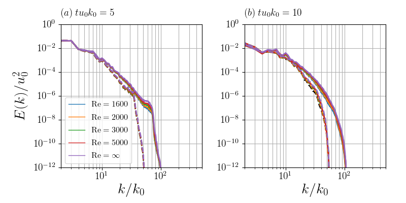
Figure 3: Energy spectra $E(k)$ of simulations at several under-resolved grid resolutions $N=128$ (solid line) and $N=64$ (dashed line) at $\mathrm{Re}=1600,2000,3000,5000$, and $\infty$ at times (a) $tu_{0}k_{0}=5$ and (b) $tu_{0}k_{0}=10$.

Next, we focus on the dissipation spectra of the simulations, which is directly obtained from the vorticity flow field. Figure 4(a) shows the dissipation spectra at $tu_{0}k_{0}=5$ has several low wavenumber peaks that are well captured by all simulations with $N=128$ or $256$ while there is lower dissipation in most modes for the $N=64$ simulations. Overall, compared to the energy spectra, the dissipation spectra is well captured at all wavenumbers especially for the $N=256$ test cases. This is an indication that these simulations can accurately resolve most of the dissipation. Near the peak dissipation at $tu_{0}k_{0}=10$, Fig 4(b) shows that grid resolution and the slope limiter start to have more effect on the resolved dissipation. The $N=256$ no-limiter case dissipation spectrum is very comparable to the DNS dissipation spectrum at most wave numbers, while the minmod limiter test case at the same resolution reveals that it can only capture the dissipation spectra at lower wavenumbers. A general trend shows that the no-limiter cases have slightly higher dissipation modes. This is an indication that the no-limiter test cases can resolve slightly more dissipation compared to the minmod limiter, but we need to investigate further. While the no-limiter can capture slightly more dissipation, it also does not add any numerical dissipation on the order of $\Delta_{x}^{2}$, so it may not be able to dissipate sufficient energy. The minmod case shows slightly lower dissipation modes in the spectra, but there is numerical dissipation that is not accounted for in this metric.

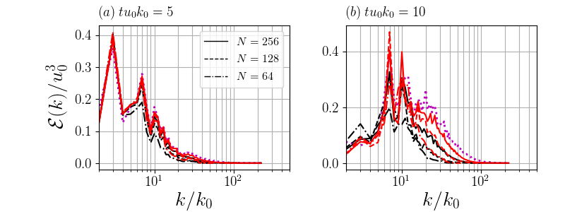
Figure 4: Dissipation spectra $\mathcal{E}(k)$ from the resolved vorticity of simulations at several under-resolved grid resolutions at $Re=1600$ at (a) $tu_{0}k_{0}=5$ and (b) $tu_{0}k_{0}=10$. Red: no-limiter, Black: minmod limiter. The magenta dotted line is the dissipation spectra from DNS results.

The total dissipation, including numerical dissipation, $\epsilon=dK/dt$, where $K=\frac{1}{2}\langle u_{i}u_{i}\rangle$ ($\langle\cdot\rangle$ indicates averaged over the computational domain) is the kinetic energy, is integrated over the entire domain and recast into a non-dimensional form, $\epsilon^{*}=\epsilon/k_{0}u_{0}^{2}$. Figure 5(a) shows the temporal evolution of the dissipation for the $N=256$ test cases where both the no-limiter and minmod limiter cases provide reasonable results compared to the DNS dissipation, which is filtered using several sharp-cutoff spectral filters with widths including $\Delta=2\Delta_{x},4\Delta_{x}$, and $8\Delta_{x}$. The filtered DNS dissipation $\widetilde{\epsilon}$ is the temporal derivative of the filtered kinetic energy $\widetilde{k}$. The filtered kinetic energy is obtained by integrating over all wavenumbers in the sharp-cutoff spectral filtered energy spectrum with different filter widths obtained from the DNS at each time step. While there are some discrepancies the peak dissipation is captured reasonably well for both cases and is comparable to the DNS filtered solution at $\Delta=2\Delta_{x}$. Figure 5(b), which shows the total dissipation for the $N=128$ cases, reveals that the minmod limiter case out performs the no-limiter case. The minmod limiter case can reasonably capture the peak dissipation, which is comparable to the $N=256$ cases and the filtered DNS dissipation at $\Delta=4\Delta_{x}$. Figure 5 (c) shows total dissipation for the $N=64$ test cases. Neither results are as reasonable as the higher resolution cases indicating that very under-resolved cases may be overly dissipative in certain regimes such as near the maximum dissipation of the Taylor-Green vortex. On the other hand, the numerical dissipation in a regime of strong coherent vortex interaction at short times or decaying turbulence at long times are more reasonably captured in very under-resolved cases. However, this low resolution case demonstrates evidence of SGS backscatter present in numerics as the numerical dissipation becomes negative around $tu_{0}k_{0}=15$. These results as well as the dissipation spectra indicate that when the flow is reasonably under-resolved, the numerical dissipation is necessary. The adequacy of the resolution will be explored below and is imperative to understand when employing ILES in general. In our scheme, the numerical dissipation has a form that is qualitatively similar to physically devised models, an aspect that offers insight in understanding the implicit SGS dissipation mechanisms.

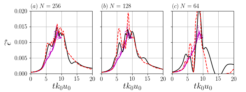
Figure 5: The filtered dissipation $\widetilde{\epsilon}^{*}$ as a function of time for (a) $N=256$, (b) $N=128$, and (c) $N=64$. Red dashed line: no-limiter, Black solid line: minmod limiter. The magenta line is the dissipation from DNS results spatially filtered with a sharp-cutoff spectral filter with several filter widths $\Delta=2\Delta_{x}$ (solid line), $4\Delta_{x}$ (dashed line), and $8\Delta_{x}$ (dotted line).

Simulations at several higher $\mathrm{Re}=1600,2000,3000,5000$, and $\infty$ reveal the effects of the numerical dissipation with diminishing viscosity for $N=128$ and $N=64$ in Figs. 6(a) and (b), respectively. For the $N=128$ between the initial condition and maximum dissipation ($0<tu_{0}k_{0}<9$), all cases share a similar numerical dissipation. The extrema are amplified by the increasing Re, which suggests that viscosity plays a role in smooth the dissipation. The effects at $\mathrm{Re}=\infty$ shows the largest discrepancies between the ILES cases and the DNS and suggest that including some physical viscosity dissipation helps stabilize the scheme. Figure 6(b) shows the $N=64$ cases with increasing Re. The cases corroborate the findings in Fig. 5(c) that a severely under-resolved case does not necessarily capture the dissipation well for all cases. This will be further explored in further below.

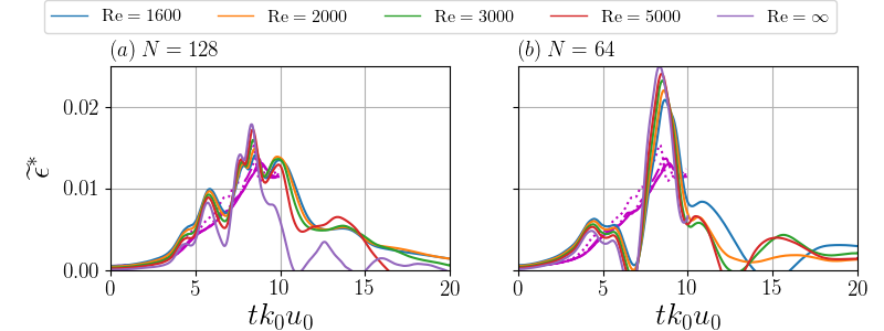
Figure 6: The filtered dissipation $\widetilde{\epsilon}^{*}$ as a function of time for (a) $N=128$ and (b) $N=64$ at $\mathrm{Re}=1600,2000,3000,5000$, and $\infty$ . The magenta line is the dissipation from DNS results spatially filtered with a sharp-cutoff spectral filter with several filter widths $\Delta=2\Delta_{x}$ (solid line), $4\Delta_{x}$ (dashed line), and $8\Delta_{x}$ (dotted line).

Next, we provide further analysis to compare the numerical dissipation of the scheme to the form of dissipation that is obtained through the modified equation analysis in section IV. Similar analysis Cerutti et al. (2000); da Silva and Pereira (2004); Zhou et al. (2020) on how the resolved vorticity field affects SGS dissipation transport has provided insights into the dynamics of the flow. We start with presenting the transport equation for the resolved enstrophy $\widetilde{\mathcal{E}}=\frac{1}{2}\langle\widetilde{\omega_{i}}\widetilde{\omega_{i}}\rangle$ that is obtained by multiplying Eqn. (4) by $\omega_{i}$ and filtering. The resolved enstrophy transport equation is given by the following:

$$\frac{\partial\widetilde{\mathcal{E}}}{\partial t}= -\underbrace{\widetilde{u_{j}}\frac{\partial\widetilde{\mathcal{E}}}{\partial x_{j}}}_{\text{I}}+\underbrace{\vphantom{\frac{\partial}{\partial_{j}}}\widetilde{\omega}_{i}\widetilde{\omega}_{j}\widetilde{s}_{ij}}_{\text{II}}+\underbrace{\nu\frac{\partial^{2}\widetilde{\mathcal{E}}}{\partial x_{j}\partial x_{j}}}_{\text{III}}-\underbrace{\nu\frac{\partial\widetilde{\omega_{i}}}{\partial x_{j}}\frac{\partial\widetilde{\omega_{i}}}{\partial x_{j}}}_{\text{IV}}-\underbrace{\widetilde{\omega}_{i}\widetilde{u}_{i}\frac{\partial\widetilde{\omega}_{j}}{\partial x_{j}}}_{\text{V}}-\underbrace{\widetilde{\omega}_{i}\frac{\partial}{\partial x_{j}}\left(R_{ij}\right)}_{\text{VI}},$$ (37)

which relates the temporal change in the resolved enstrophy to spatial changes in the vorticity, velocity, and SGS vorticity stress tensor. The equation contains several mechanisms that balance the temporal change in resolved enstrophy: I.) convection, II.) amplification by vortex stretching, III.) diffusion by viscous effects, IV.) dissipation by viscous effects, V.) diffusion by divergence modification, and VI) SGS dissipation and SGS diffusion. Term VI can be expanded into two terms as follows:

$$\widetilde{\omega}_{i}\frac{\partial}{\partial x_{j}}\left(R_{ij}\right)=\frac{\partial}{\partial x_{j}}(\widetilde{\omega_{i}}R_{ij})-R_{ij}\frac{\partial\widetilde{\omega_{i}}}{\partial x_{j}},$$ (38)

where the first term is the diffusion by SGS modes and the second term is the SGS dissipation. This expansion allows us to investigate the SGS dissipation by terms that are present in the modified equation. We discretized each derivative (in space and time) using standard 3 point second order central differencing. Note that vorticity does not need to be discretized, because it is the solution variable. Every term in Eqn. (37) except term VI can be directly calculated from the instantaneous flow. However, because it is necessary to balance Eqn. (37), we can find term VI, which gives us the exact numerical SGS dissipation and SGS diffusion due to the scheme and slope limiter. Figure 7(a) shows the temporal evolution of each term in Eqn. (37) for the test case with $N=64$ employing the minmod limiter. Near the initial time, the temporal change in the enstrophy is dominated by the amplification of vortex stretching. At this time, the vortical structures are large and nearly resolved by the grid resolution and there is very little SGS interactions. However, as the flow progresses towards the transition to turbulence around $tk_{0}u_{0}=5$, the SGS term begins to increase as a balance to the amplification by vortex stretching. Around this time, there is non-negligible viscous dissipation, however, the other terms are small compared to the vortex stretching and SGS terms. This trend continues towards the maximum dissipation time near $tk_{0}u_{0}=9$ and after as the turbulence begins to decay. The trend that vortex stretching balances the SGS dissipation is consistent with experiments of high Reynolds number turbulence Cerutti et al. (2000) with multi-probe hot-wire measurements. Overall, the SGS term is balanced by the vortex stretching, which indicates that a majority of the dissipation is provided by the numerical method not the viscosity.
In Fig. 7(b) the SGS dissipation and SGS diffusion term (VI) in Eqn. (37) are compared with the modeled SGS dissipation and production (i.e. modified equation sub-grid dissipation and diffusion) that uses $R_{ij}=R^{t}_{ij}+R^{g}_{ij}+R^{h}_{ij}$ from Eqns. (35), (32), and (34), respectively. The temporal evolution of the modified equation SGS dissipation and SGS diffusion has a similar trend as the numerically calculated term while there are some discrepancies near the peak dissipation. These discrepancies arise from a) the simplified calculation of the modified equation by not incorporating the exact limiter definition, and b) truncation of the final modified equation to only second-order accurate terms. The modeled SGS dissipation and modeled SGS diffusion are obtained through Eqn. (38), which shows that SGS dissipation is the dominating term compared to the diffusion.

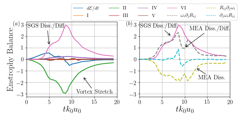
Figure 7: (a) The temporal evolution of terms in the enstrophy transport equation for the $N=64$ test case with minmod limiter. (b) The temporal evolution of the calculated SGS dissipation and diffusion and the temporal evolution of the SGS dissipation and diffusion obtained from the modified equation for the $N=64$ test case with minmod limiter.

The balance of enstrophy is also investigated at a higher grid resolution in Fig. 8(a) with $N=128$ and the minmod limiter. The temporal evolution of the amplification by vortex stretching term is the dominant term in the enstrophy balance. Compared the $N=64$, the amount of the viscous dissipation is increased, which is expected because the higher grid resolution resolves more viscous dissipation. The increased viscous dissipation acts as an offset for the SGS dissipation and SGS diffusion term, which is comparably less for all simulated time compared to the corresponding terms in the $N=64$ test case. Figure 8(b) shows the comparison of the calculated SGS dissipation and diffusion term with the modeled SGS dissipation and SGS diffusion. At this resolution, the model elucidated from the modified equation analysis is shown to be well represented because higher order terms in the modified equation become smaller with higher grid resolution. As with the coarser grid resolution the SGS dissipation is dominant compared to the SGS diffusion. Overall, the enstrophy transport equation analysis shows that the numerical results and the form of the implicit SGS model derived from the modified equation analysis are similar and provides validation for the modified equation analysis for this scheme.

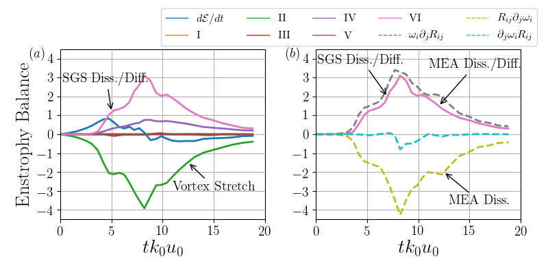
Figure 8: (a) The temporal evolution of terms in the enstrophy transport equation for the $N=128$ test case with minmod limiter. (b) The temporal evolution of the calculated SGS dissipation and diffusion and the temporal evolution of the SGS dissipation and diffusion obtained from the modified equation for the $N=128$ test case with minmod limiter.

The modified equation SGS dissipation and diffusion can be separated into three different terms based on Eqns. (32), (34) and (35) developed directly from the modified equation. This allows us to identify which mechanism dominants the dissipation in the ILES. Figure 9(a) shows the temporal evolution of the three terms for the $N=64$ test case with the minmod limiter. Overall the modified equation SGS dissipation is driven by terms similar to a tensor-gradient model. Similarly, for the $N=128$ test case with the minmod limiter shown in Fig. 9(b), the tensor-gradient terms in Eqn. (32) are the dominant mechanism for dissipation. In general, these SGS models with tensor-gradient are not overly dissipative and normally are paired with other models. This is consistent with the SGS dissipation shown herein. The modified equation terms similar to a hyper-viscosity model in Eqn. (34) are shown to contribute to the total SGS dissipation, which enables the total modified equation SGS dissipation to have a similar temporal evolution as the calculated SGS dissipation (term VI). The SGS dissipation contribution from Eqn. (35) is shown to relatively less significant for both resolutions.

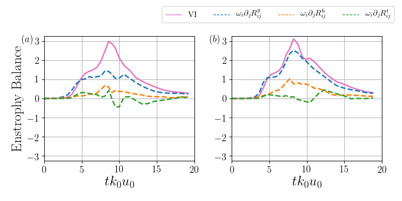
Figure 9: The temporal evolution enstrophy transport of components of the SGS dissipation and diffusion obtained from modified equation in Eqns. (32), (34) and (35) for (a) $N=64$ and (b) $N=128$ test cases with minmod limiter.

Figure 10(a) shows the enstrophy balance for the $N=64$ with no-limiter case to show the temporal evolution of the transport of enstrophy when no limiter is employed in the scheme, which limits the numerical dissipation. Similar to the limited cases presented in Fig. 7, amplification by vortex stretching dominants the evolution of enstrophy, but is significantly larger than the limited cases. Furthermore, terms IV and V are also augmented compared to the limited case by the lack of limiter and pathway for dissipation. This has a large influence on the balance and the SGS dissipation/diffusion term. This term is significantly higher than than the limited case and corroborates the high numerical dissipation observed in Fig. 5(c). Similarly, the $N=128$ case shows that the amplification of vortex stretching is elevated by the lack of limiting. This affects the enstrophy balance by increasing the remainder calculated in the SGS dissipation/diffusion.

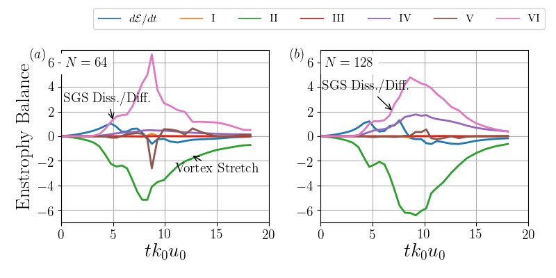
Figure 10: The temporal evolution of terms in the enstrophy transport equation for (a) $N=64$ and (b) $N=128$ test cases with no-limiter.

Figure 11 compares the SGS dissipation $\epsilon_{SGS}$ with the expected SGS dissipation obtained through DNS. The latter is obtained by filtering the dissipation spectra Fig. 4 using a sharp-cutoff spectral filter with a length scale $2\pi/(N/4+1)$, where $N$ is the grid resolution for each case. Figures 11(a), (b), and (c) show that the SGS dissipation for the $N=256,128$, and $64$ cases, respectively. As expected, as the length scale of the filter is increased, the total SGS dissipation increases for both the DNS and ILES. The SGS dissipation from both ILES cases (minmod and no-limiter) are lower than the DNS dissipation as expected based on the dissipation spectra, which indicated that the total resolved dissipation smaller than the filter scale is relatively small. The SGS dissipation obtained through the modified equation analysis for the $N=128$ and $N=64$ cases with the minmod limiter $\omega_{i}\partial_{j}R_{ij}$ is included in Figs. 11(b) and (c). The SGS dissipation is relatively similar to that from the filtered DNS for $N=128$. It is however, under-predicted for $N=64$ . This provides further evidence with the Fig. 5(c) that more analysis and clarification is needed especially in the low resolution limit.

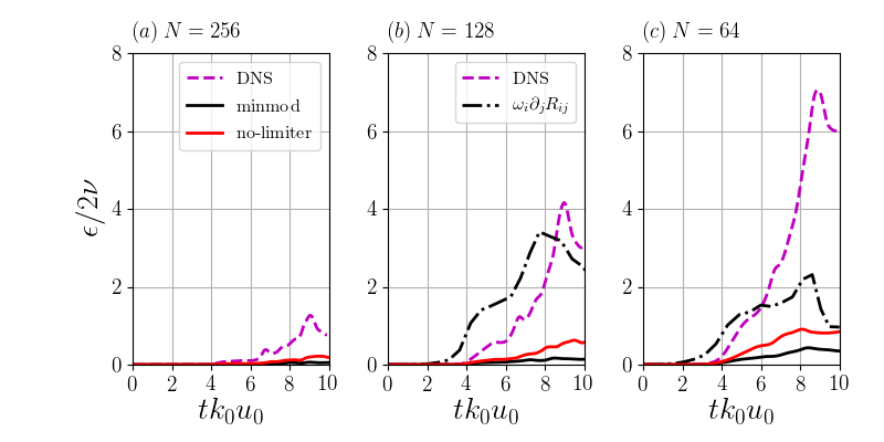
Figure 11: The SGS dissipation $\epsilon_{SGS}$ for the Taylor-Green vortex for (a) $N=256$, (b) $N=128$, and (c) $N=64$. The SGS dissipation obtained from the modified equation analysis is shown for the $N=128$ and $N=64$.

Next, to further understand the implicit numerical dissipation and SGS model derived from the modified equation analysis we compare several terms of the modified equation to the well-known Smagorinsky model. A Smagorinsky model Smagorinsky (1963) was developed in Ref. Mansfield et al. (1998) for the VTE and can used for closure of $R_{ij}$:

$$\frac{\partial R_{ij}}{\partial x_{j}}=g_{i}=-\frac{\partial}{\partial x_{j}}\left(\nu_{t}\frac{\partial\omega_{i}}{\partial x_{j}}\right)-\frac{\partial\nu_{t}}{\partial x_{j}}\frac{\partial\omega_{j}}{\partial x_{i}}.$$ (39)

The eddy viscosity $\nu_{t}$ is given by

$$\nu_{t}=C_{s}{\Delta}^{2}|\widetilde{S}|,$$ (40)

where $\widetilde{S}_{ij}$ is the filtered strain-rate tensor, $C_{s}$ is the Smagorinsky constant and $|\widetilde{S}|=(2\widetilde{S}_{ij}\,\widetilde{S}_{ij})^{\frac{1}{2}}$. While the implicit model is shown by modified equation analysis to consist of several terms (Eqns. (35), (32), and (34)) and provide implicit SGS vorticity stress on all tensor element, the comparable Smagorinsky model creates an anti-symmetric SGS vorticity stress tensor.
Additional LES cases are simulated using the explicit model in Eqn. (39). No limiter is used in the upwind based scheme to ensure that the dissipation is enabled through the explicit model; however, there is still interaction between the scheme dissipation and explicit model dissipation. Several Smagorinsky constants are employed including $C_{s}=0.1$ and $0.3$, where the former is used in Ref. Mansfield et al. (1998) with a vortex particle method discretization. Simulations are performed at $N=64$ and $128$ resolution of the Taylor-Green vortex at $\mathrm{Re}=1600$ to compare to the present results. Figures 12(a) and (b) show the numerical filtered dissipation $\widetilde{\epsilon}^{*}$ at $N=64$ and $N=128$, respectively. The dissipation is shown to be affected significantly by the Smagorinsky constant. In fact, the constant used previous studies is shown to be out performed by the ILES. The higher constant, especially in $N=64$ performs slightly better. The discrepancies are affected by the interactions of the modified equation of the vorticity transport scheme, even if no limiter is employed, and the SGS model. Further insights into the performance of explicit LES compared to the present implicit model is shown in the enstrophy transport analysis in Figs. 12(c) and (d) for the $N=64$ and $N=128$, respectively. Results from the explicit LES model suggest that the value of the model coefficient produces high variability for the SGS dissipation. Moreover, a priori tests of forced homogeneous, isotropic turbulence Mansfield et al. (1998) reveal that both vorticity convection and vortex stretching contribute to sub-grid scale dissipation, but the explicit eddy-viscosity model does not capture the contribution from vortex stretch adequately. While the variability may be reduced with a dynamic model Mansfield et al. (1998); Germano et al. (1991), the overall simplification, deterministic dissipation through the modified equation, consistent integration both the vorticity convection and vortex stretching, and reduced computational effort of the implicit approach are desirable qualities for a scheme. Furthermore, ILES has been described by one constant—typically the effective viscosity Zhou and Thornber (2016)—to quantify the observed behavior of the simulated flow field.

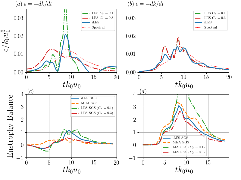
Figure 12: The filtered dissipation $\widetilde{\epsilon}^{*}$ as a function of time for (a) $N=64$ and (b) $N=128$ comparing test case with minmod limiter, two explicit LES cases with $C_{s}=0.1$ and $0.3$, and DNS results from a spectral method. The temporal evolution of the calculated SGS dissipation and diffusion obtained from the present method, the modified equation, and Smagorinsky model for explicit LES with grid discretization of (c) $N=64$ and (d) $N=128$.

Finally, we analyze the scheme by attempting to provide methodology to characterize the flow field in terms of a numerical effective Reynolds number $\textrm{Re}_{f}$. In the previous analysis, we demonstrated that the numerical dissipation of the present schemes and the dissipation predicted by the modified equation are similar. In what follows, we provide methodology to characterize the flow in order to determine if the simulation is sufficiently resolved to provide an accurate solution. This is particularly important considering the $N=64$ simulations where numerical dissipation is considerably different from DNS dissipation. If the simulation is not sufficiently resolved then we provide information on what the simulation physically solved. In coarse-grained simulations, such as LES either explicit or implicit, where small scales are not directly solved but are modeled, the $\textrm{Re}_{f}$ can be used to interpret what the simulation physically solved. The methodology is based on the analysis of an ILES Euler scheme of turbulence flows by Ref. Zhou et al. (2014). For incompressible flows with sufficiently fine grid resolution to be considered a DNS, the numerical dissipation $-dK/dt$ and resolved dissipation $\epsilon_{\mathcal{E}}=2\nu\langle\omega_{i}\omega_{i}\rangle$ are equal. This means that the scales impacted by the numerics of scheme are in only in a narrow band of high wavenumbers dominated by the viscous scales. In the under-resolved simulations presented herein, the ratio of the resolved enstrophy and dissipation is used to characterize the $\textrm{Re}_{f}$ as the following:

$$\textrm{Re}_{f}=\frac{u_{0}}{k_{0}\nu_{f}}=\frac{\langle\omega^{*}_{i}\omega^{*}_{i}\rangle}{\epsilon^{*}}.$$ (41)

Figure 13(a) shows the temporal evolution of $\textrm{Re}_{f}$ of several test cases including some additional test cases with different $\textrm{Re}=u_{0}/k_{0}\nu$ than presented above in order to understand some general trends. The additional Re included are 800, 2000, 3000, 5000, and an inviscid case where the $\textrm{Re}=\infty$. In each case, the initial $\textrm{Re}_{f}$ is near the Re indicating that the initial numerical dissipation and resolved dissipation are equal. However, the $\textrm{Re}_{f}$ decreases as the enstrophy increases towards a maximum. The grid resolution of each case has an effect on how the $\textrm{Re}_{f}$ decreases where the largest decreases can be attributed to the lowest grid resolution cases. In Fig. 13(b), the $\textrm{Re}_{f}$ is selected at $t=5$ when the transition to turbulence is occurring. The $\textrm{Re}_{f}$ is observed to be a function of the physical viscosity while the grid resolution has a secondary effect. However, the $\textrm{Re}_{f}$ lower than the Re, which indicates there is noticeable discrepancy in the numerical dissipation and the resolved dissipation. The $\textrm{Re}_{f}$ is selected at the location of maximum dissipation for each case and is shown in Fig. 13(c). The results show that the grid resolution has the largest effect on $\textrm{Re}_{f}$. The $\textrm{Re}_{f}$ increases with the grid resolution. Regardless of the slope limiter or Re, all cases show similar behavior. This suggests that the numerical dissipation is highly affected by the grid resolution compared to the effects of the viscous diffusion or limiting in the flux functions of the present scheme for the Taylor Green vortex. We observe that the $N=128$ cases, which have a closer $\textrm{Re}_{f}$ to 800 than 1600, can be reasonably compared to the results for the $\textrm{Re}=800$ in some parts of the evolution of the flow. At the highest resolution case $N=256$, secondary effects of the Re begin to have a larger effect.

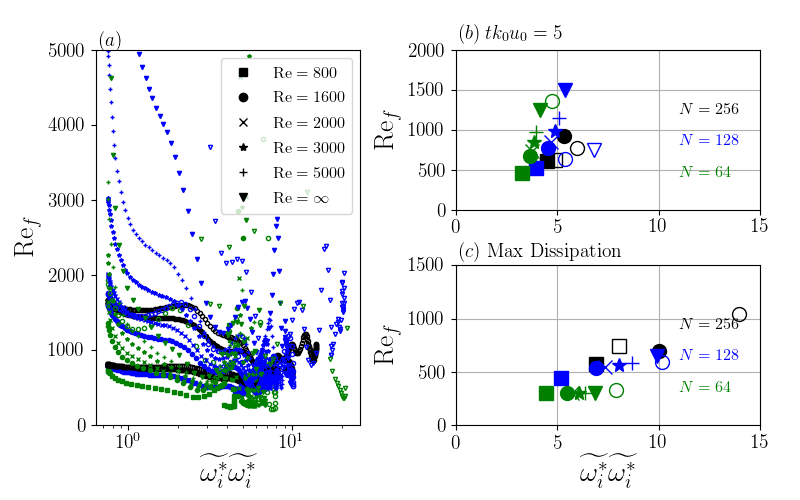
Figure 13: The effective Re, $\textrm{Re}_{f}$, as a function of twice the enstrophy throughout the runtime of the simulations for several grid resolutions and viscosities. The $\textrm{Re}_{f}$ at (b) $t=5$ and (c) maximum dissipation.

Next, we can use the ratio of the numerical dissipation and the resolved dissipation to create an effective length scale as follows:

$$\Delta x_{f}=\frac{\epsilon^{1/2}}{\left(\widetilde{\omega_{i}}\widetilde{\omega_{i}}\right)^{3/4}}.$$ (42)

The effective length scale is compared with the Kolmogorov length scale $\eta$ provide by the DNS at a $\textrm{Re}=1600$ in Fig. 14. The temporal evolution of the effective length scale indicates that before the transition to turbulence, the flow field is relatively resolved. However, as the large structures begin to break down, the grid is no longer sufficiently fine to resolve the flow and the effective length scale become larger than the Kolmogorov scale. The grid resolution has a large effect on the evolution of the effective length scale.

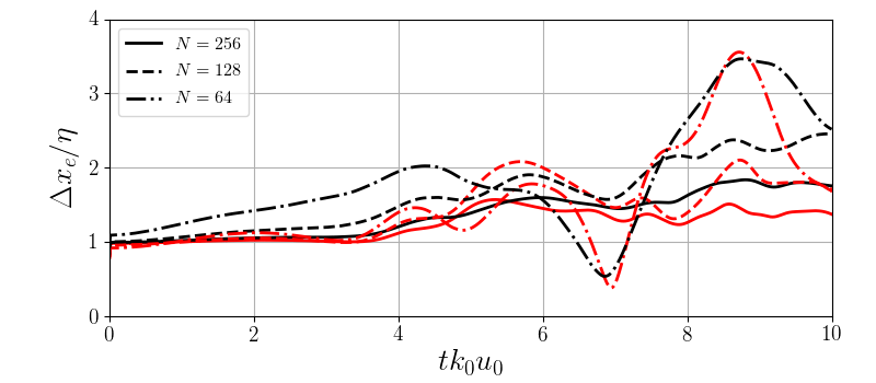
Figure 14: The ratio of the effective grid spacing and Kolmorgorov lengthscale (from DNS) $\Delta x_{f}/\eta$ for the $\textrm{Re}=1600$ cases. Red: no-limiter, Black: minmod limiter.

Further analysis into $\textrm{Re}_{f}$ of the simulations allows us to interpret the effective viscosity $\nu_{f}$ with the Taylor micro-scale $\lambda$ which is calculated as follows:

$$\lambda=\frac{1}{3}\sum^{3}_{i}\sqrt{\langle u_{i}u_{i}\rangle/\langle\frac{\partial u_{i}}{\partial x_{i}}\frac{\partial u_{i}}{\partial x_{i}}\rangle}.$$ (43)

The effective Taylor micro-scale $\textrm{Re}_{\lambda}=u^{\prime}\lambda/\nu_{f}$. Many studies on high-Re turbulence have investigated the relationship between the energy containing eddies in flows with the dissipation especially using turbulence-resolving DNS or experiments Kaneda et al. (2003); Falkovich (1994); Wang et al. (1996); Sreenivasan (1998). From these efforts, we are able to conclude that the time scale of the energy-containing eddies $u^{\prime}/L$ are on the same magnitude as the time scale of the dissipation rate $\epsilon/u^{\prime 2}$, where $u^{\prime}$ is the characteristic velocity scale and $L$ is the characteristic length scale. This key finding is especially beneficial for success with under-resolved simulations where by resolving large energy-containing eddies, there is some understanding of the magnitude of the dissipation just based on resolved characteristics. Furthermore, the DNS studies showed that with a sufficiently high $\text{Re}_{\lambda}$, the flow reaches a minimum state Zhou (2007) where turbulence seems to exhibit self-similar behavior. The minimum state of turbulence flows where the time scale of the large scales and dissipation in terms of $\textrm{Re}_{\lambda}$ can be as low as $\textrm{Re}_{\lambda}>100$ Sreenivasan (1984); Dimotakis (2000) or $\textrm{Re}_{\lambda}>200$ Kaneda et al. (2003); Sreenivasan (1998). For the Taylor-Green vortex case with $\textrm{Re}=1600$, the maximum $\textrm{Re}_{\lambda}=140$ Brachet (1991). This implies that in order to reach some self-similarity of small-scale turbulence the flow must have sufficient separate of scales, and the dissipation must occurs away from the large scales in the spectral sense. Ref. Zhou et al. (2014) used this criteria in order to characterize ILES schemes for velocity-pressure formulation to see if a minimum state is reached. Furthermore, well-known relationships for $\textrm{Re}_{\lambda}$ to a large-scale $\textrm{Re}_{L}$ exist. Several studies have pointed towards $\textrm{Re}_{L}\sim\textrm{Re}^{2}_{\lambda}$ Tennekes and Lumley (1972); Sagaut and Cambon (2008).
We present details on the characteristics of several of the Taylor-Green simulations in Table 1, which shows the effective Re at transition to turbulence ($t=5$), maximum dissipation ($t\approx 9$), and decaying turbulence ($t=15,20$). Here, we calculate the characteristic velocity as the rms (root-mean-square) of the velocity fluctuations $u^{\prime}=\langle(\frac{1}{3}u_{i}u_{i})^{1/2}\rangle$. The high-resolution cases with $N=256$ show that the limiter has minor effects on $\textrm{Re}_{f}$ as also shown in Fig. 13. While only at the transition stage has the flow field reached a sufficiently high $\textrm{Re}_{\lambda}$, this is consistent with ILES simulations with for the Euler equations Zhou et al. (2014). The DNS has an initial $\mathrm{Re}_{\lambda}=55$ which increases to the maximum $\textrm{Re}_{\lambda}=140$ Brachet (1991); Zhou and Thornber (2016) around $t=9$. $\mathrm{Re}_{\lambda}\approx 100$ at larger times $t>10$ as the turbulence decays. In the $N=128$ test cases, the numerical dissipation provided by the minmod limiter has more effects while in the $N=64$, the $\textrm{Re}_{f}$ remains relatively low and does not provide positive results during turbulence decay indicating that the grid resolution is not high enough or the dissipation is not enough for this flow.

Table 1: Effective Re for ILES of Taylor-Green Vortex

$N$	Limiter	$t$	$Re_{f}=\frac{u_{0}}{k_{0}\nu_{f}}$	$\Delta x_{f}$	$Re_{\lambda}=\frac{u^{\prime}\lambda}{\nu_{f}}$	$Re_{L}\sim Re_{\lambda}^{2}$
256	No-limiter	5.00	774	2.30$\times 10^{-2}$	98	9692
		9.03	1048	1.60$\times 10^{-2}$	58	3407
		15.00	1624	1.61$\times 10^{-2}$	47	2251
		20.00	1704	1.98$\times 10^{-2}$	43	1871
	Minmod	5.00	923	2.16$\times 10^{-2}$	122	14991
		8.30	698	2.13$\times 10^{-2}$	52	2711
		15.00	1135	2.08$\times 10^{-2}$	47	2226
		20.00	1283	2.30$\times 10^{-2}$	45	2048
128	No-limiter	5.00	639	2.60$\times 10^{-2}$	86	7527
		8.49	589	2.31$\times 10^{-2}$	42	1819
		15.00	1328	1.92$\times 10^{-2}$	45	2100
		20.00	1596	2.04$\times 10^{-2}$	41	1725
	Minmod	5.00	769	2.47$\times 10^{-2}$	109	11956
		8.29	533	2.67$\times 10^{-2}$	52	2755
		15.00	856	2.57$\times 10^{-2}$	39	1559
		20.00	1313	2.39$\times 10^{-2}$	47	2212
64	No-limiter	5.00	1356	1.84$\times 10^{-2}$	203	41296
		8.23	329	3.28$\times 10^{-2}$	38	1503
	Minmod	5.00	667	2.80$\times 10^{-2}$	104	10965
		8.33	303	3.75$\times 10^{-2}$	46	2144

V.2 Forced Isotropic Turbulence

Next, we consider the numerical experimentation of isotropic turbulence simulation employing a forcing scheme developed for linear forced turbulence in physical space Rosales and Meneveau (2005). Forced isotropic turbulence provides test cases that allow for velocity and vorticity statistics to be collected over the simulation, which are used to assess the ILES dissipation and ability to capture turbulence statistics. A forcing term $\widetilde{\bm{f}}=\nabla\times\epsilon_{0}/3u^{\prime 2}\bm{u}$, where $\epsilon_{0}$ is a constant energy injection and $u^{\prime}=\left(\frac{3}{2}\langle K\rangle\right)^{1/2}$ is the rms (root-mean-squared) velocity updated throughout the simulation, is included in Eqn. (4) to maintain a nearly constant energy after an initial transient time. The energy injection constant is $\epsilon_{0}=5\times 10^{-5}$. The simulation cases are initialized using the conditions for isotropic turbulence. It is simulated from an initial condition, which quickly decays into fully-developed turbulence, given in Refs. Mansour and Wray (1994) and Rogallo (1981) where the initial energy spectrum takes the form:

$$E(k,0)=\frac{3}{2A}\frac{1}{k_{p}^{\sigma+1}}k^{\sigma}\exp\left(-\frac{\sigma}{2}\left(\frac{k}{k_{p}}\right)^{2}\right),$$ (44)

where $k_{p}$ is the wavenumber at which $E(k,0)$ is maximum, $\sigma$ is parameter, and $A$ is $\int_{0}^{\infty}k^{\sigma}\exp(-\sigma k^{2}/2)dk$. A flow is initialized with $\sigma=4$ and $k_{p}=3$. The $\nu=0.0007$ gives a initial Reynolds number based on the length of the side domain, $2\pi$, and the initial velocity fluctuations of $\textrm{Re}=6\times 10^{3}$. Grid resolutions are employed in the $2\pi$-sided periodic box with the number of grid cells per dimension $N=256,128,64$, and $32$ with a minmod limiter for all resolutions. An additional no-limiter case is employed for the $N=256$ resolution based on results above which show that the $N=256$ is nearly resolved for the present initialization.
Several studies Zhou et al. (2014); Wachtor et al. (2013); Fureby and Grinstein (2002) have employed forced turbulence simulations to examine the turbulence statistics especially to see sensitivities the velocity, vorticity, and strain rates have for ILES with different grid resolutions. It has been observed in Ref. Zhou et al. (2014) for ILES that above a mixing transition of $\textrm{Re}_{\lambda}>100$ Dimotakis (2000), the behavior of the turbulence statistics in terms of velocity probability density functions (PDFs) begin to approach asymptotic Re statistics. Figure 15 shows the longitudinal and transverse fluctuating velocity gradients with a comparison to DNS Jiménez et al. (1993) and grid turbulence experimental measurements Castaing et al. (1990). The present simulations capture the turbulence statistics, especially, the high probability statistics well for all grid resolutions. The tails of the PDFs, which represent only a small fraction of the solution correspond well with higher $\textrm{Re}_{\lambda}$ DNS and experimental cases, which suggests that the numerical dissipation in the scheme may be appropriate for simulating high Re turbulence cases in which intermittency and non-Gaussian behavior at the tail of PDFs are observed. The negative bias of the longitudinal derivative of the fluctuating velocity is similar to results present in DNS and experimental flow field statistics. The PDF of the transverse derivative of the fluctuating velocity shown in Fig. 15 demonstrates the convergence of the velocity towards non-Gaussian behavior observed for this quantity. The turbulence statistics indicate that there is convergence towards high Re turbulence statistics.

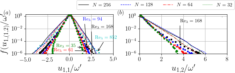
Figure 15: Longitudinal (left) and transverse (right) velocity gradient probability density functions normalized by the rms vorticity $\omega^{\prime}$ with several grid resolutions. Markers indicate PDFs captured from DNS results from Ref. Jiménez et al. (1993) are at $\textrm{Re}_{\lambda}=35,61,94$ and $168$ and Experimental measurements from Ref. Castaing et al. (1990) are at $\textrm{Re}_{\lambda}=852$. Each PDF is labeled.

Figure 16(a) show the near Gaussian behavior, similar to flow fields from DNS results, of the velocity fluctuations, which show asymptotic convergence as the grid resolution increases. This also suggests that the effective Re is increasing with the grid resolution as seen in the Taylor-Green vortex. The statistics for the magnitude of the vorticity fluctuations are shown in Fig. 16(b), which suggests that vorticity statistics are better represented compared to the velocity statistics at lower grid resolutions and for this particular Re. Interestingly, this is not seen ILES of velocity-pressure formulations Zhou et al. (2014), which may suggest that the present scheme designed to preserve vorticity may enhance the ability of lower grid resolution cases to capture some vorticity statistics more efficiently and DNS simulations from Ref. Jimenez and Wray (1998) have relatively low $\textrm{Re}_{\lambda}$. Next, we focus on statistics related to the resolved enstrophy transport equation shown in Eqn. (37). The PDF of the vortex stretching, $\sigma_{ij}=\omega_{i}s_{ij}\omega_{j}/|\omega|^{2}$, shows the convergence of the high probability portion of the PDF and tails that correspond well with different Re. Furthermore, the PDF of the strain rate magnitude in Fig. 16(d) shows similar behavior. Overall, the velocity and vorticity statistics display that the turbulence characteristics have asymptotic convergence and tails of the PDF resemble higher Re statistics with increasing grid resolution.

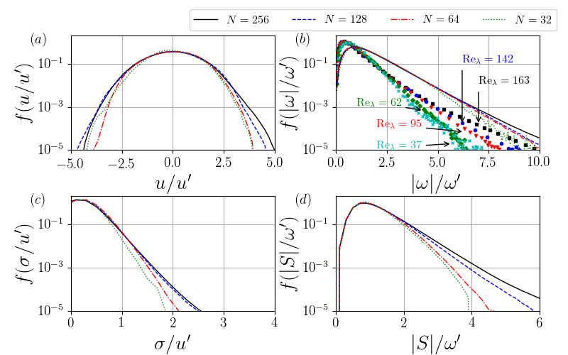
Figure 16: (a) Velocity magnitude, (b) vorticity magnitude, (c) vortex stretching, and (d) strain rate magnitude probability density function normalized by the rms vorticity $\omega^{\prime}$ of forcing case for several grid resolutions. The case $N=256$ with no-limiter is shown as a solid cyan line. Marked indicate DNS results from Ref. Jimenez and Wray (1998) are at $\textrm{Re}_{\lambda}=37,62,95,142$ and $168$. Each PDF is labeled.

The effect of numerics of the ILES on the correlation of turbulence statistics is shown in Fig. 17. First, Fig. 17(a) shows that the joint PDF of the vorticity magnitude and the strain rate magnitude $|S|$. The correlation between the two quantities reveals some convergence towards in the tails of the PDF for the three lowest grid resolutions. However, because the $N=256$ cases employs a central difference for the limiter, due to it being nearly resolved, there is a difference between this case and the other three. Furthermore the correlations between the vorticity and vortex stretching and the strain rate magnitude and stretching in Figs. 17(b) and (c) respectively show similar behavior. The statistics indicate that there is high probability that the grid resolution does not have an effect on the statistics of the flow field, while the outlying statistics have some dependence on the resolution of the simulation.

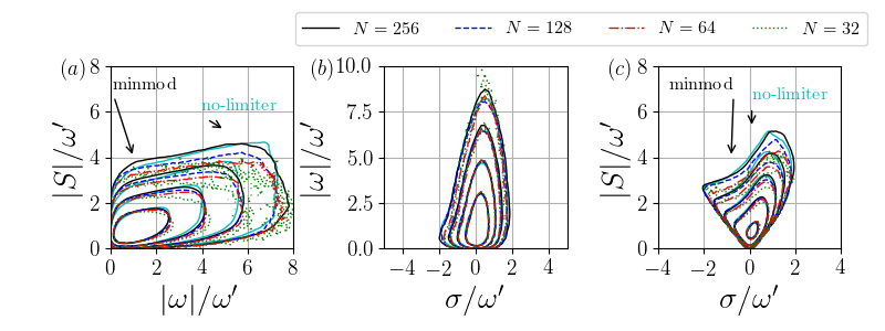
Figure 17: Turbulence statistics of the forced turbulence simulations for grid resolutions of $N=256,128,64$ and $32$. Contour lines for each plot are shown at $\{10^{0},10^{-1},10^{-2},10^{-3}\}$.

In order to further assess the implicit method, invariants of the velocity gradient Cantwell (1993), which is related to turbulence dissipation, are analyzed. The three invariants of the velocity gradient $A_{ij}=\frac{\partial u_{i}}{\partial x_{j}}$ are given as follows:

$$P =-A_{ii}=0$$ (45)

$$R =-\frac{1}{2}A_{ij}A_{ji}$$

$$Q =-\frac{1}{3}A_{ij}A_{jk}A_{ki}$$

Because the first invariant $P$ is zero for an incompressible flow, the velocity gradient is completely determined by the second and third invariants, $R$ and $Q$, respectively. The invariants determine the local flow topology and indicate stretching and stability.
Figure 18(a) and (b) shows the joint PDF for the $N=64$ and $N=128$ test cases, respectively. The invariants are determined at every grid points at $t/\tau=10$, where $\tau=u^{\prime 2}/\epsilon$ is the eddy-turnover time. Both cases reveal a joint PDF this consistent with previous studies of homogeneous turbulence Cantwell (1993). Furthermore, the invariants calculated in each simulation corroborate the PDFs of the turbulence statistics in that the overall statistics are captured independent of grid resolution. Increased grid resolution increases the appearance of outliers and are be associated with intermittency, which should be expected by resolving smaller velocity fluctuations.

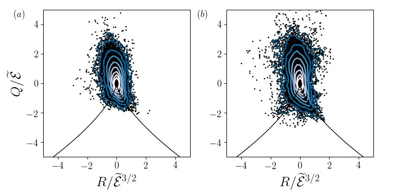
Figure 18: Joint PDF of velocity gradient invariants $Q$ and $R$ normalized by the resolved enstrophy $\widetilde{\mathcal{E}}$ of the forced turbulence simulations for grid resolutions of (a) $N=64$ and (b) $N=128$. Contour lines for each plot are shown in log-space between $0$ and $10^{-5}$.

Next, three new simulations are introduced with a grid resolution $N=64$ but with different initial $\mathrm{Re}=8.4\times 10^{3},4.2\times 10^{4}$, and $4.2\times 10^{5}$. This is obtained by changing the kinematic viscosity. All other conditions and forcing remain consistent with the $N=64$ test case at $\mathrm{Re}=6\times 10^{3}$. Figure 19(a) shows the longitudinal velocity gradient PDF of the four $N=64$ simulations. As the Re number increases, the tails of PDF trend closer to the high $\mathrm{Re}_{\lambda}$ results obtained from DNS and experimental measurements. Furthermore, Fig. 19(b), showing the transverse velocity gradient PDF, suggests similar, yet non-monotonic Akselvoll and Moin (1996), convergence as the Re number increases. The higher Re demonstrate that a larger scale separation compared to lower Re is achieved at a minimum state Zhou et al. (2014) such that the turbulence statistics become asymptotic. The velocity gradient statistics as a function of Re corroborate the statistics as a function of grid resolution (Fig. 15) to indicate that asymptotic turbulence and dissipation behavior with ILES and VTE scheme can be realized through combination of both high initial Re and sufficient grid resolution. This ensure that the turbulence will have a sufficient separation of scales.

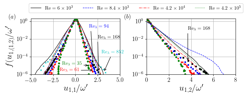
Figure 19: Longitudinal (left) and transverse (right) velocity gradient probability density functions normalized by the rms vorticity $\omega^{\prime}$ for grid resolutions of $N=64$ at several initial Re numbers. Markers indicate DNS results from Ref. Jiménez et al. (1993) are at $\textrm{Re}_{\lambda}=35,61,94$ and $168$. Experimental measurements from Ref. Castaing et al. (1990) are at $\textrm{Re}_{\lambda}=852$. Each PDF is labeled.

The velocity gradient invariants of the four different Re cases at $N=64$ are shown in Fig. 20. These statistics show that as the Re number increases, the joint PDF of the invariants resembles the canonical ‘teardrop’ shape more definitely. The Q-R plot at higher Re compared to $\mathrm{Re}=6000$ resemble the $N=128$ case shown in Fig. 18(b) more as the Re increases. This further suggests that once a minimum state is reached, statistics become asymptotic.

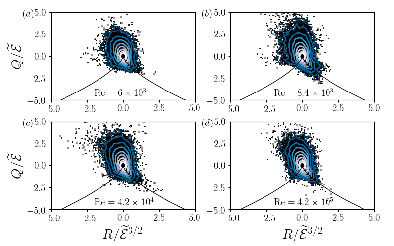
Figure 20: Joint PDF of velocity gradient invariants $Q$ and $R$ normalized by the resolved enstrophy $\widetilde{\mathcal{E}}$ of the forced turbulence simulations for grid resolutions of $N=64$ at several Re numbers. Contour lines for each plot are shown in log-space between $0$ and $10^{-5}$.

The balance of terms in enstrophy transport equation introduced in Eqn. (37) is shown in Fig. 21(a) for the $N=64$ case in order to assess the modified equation analysis with forced turbulence. Similar to the Taylor-Green vortex, the amplification via vortex stretching is balanced by SGS dissipation and diffusion. Figure 21(b) shows that the modified equation SGS dissipation and diffusion are consistent with the calculated profile throughout the simulation. This is a further indication that the implicit model obtained through the modified equation can be used to describe the dissipation of the scheme.

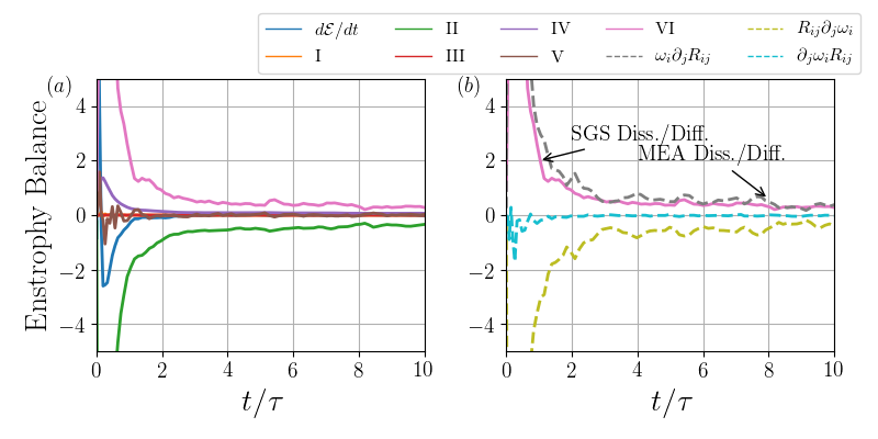
Figure 21: (a) The temporal evolution of terms in the enstrophy transport equation for the $N=64$ test case with minmod limiter. (b) The temporal evolution of the calculated SGS dissipation and diffusion and the temporal evolution of the SGS transfer and diffusion obtained from the modified equation for the $N=128$ test case with minmod limiter.

The accuracy of the modified equation SGS dissipation and diffusion at $N=128$ is corroborated in Fig. 22. In this case, the enstrophy amplification by vortex stretching is offset by both the SGS dissipation and viscous dissipation. At this resolution, there is significantly more resolved viscous dissipation than the $N=64$ case. The calculated SGS dissipation and diffusion is shown to be very similar to the modified equation SGS dissipation and diffusion throughout the simulation.

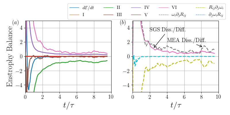
Figure 22: (a) The temporal evolution of terms in the enstrophy transport equation for the $N=128$ test case with minmod limiter. (b) The temporal evolution of the calculated SGS dissipation and diffusion and the temporal evolution of the SGS transfer and diffusion obtained from the modified equation for the $N=128$ test case with minmod limiter.

Finally, we examine the average energy spectra over the final half of the simulations in Fig. 23. The energy spectra indicate that there is a well-captured low wavenumber regime of all the simulations regardless of the grid resolution. A zoomed-in plot in the low wavenumber region before the inertial range show that both the $N=256$ and $128$ spectra are nearly converged together, while the modes for the $N=64$ grid resolution approaches similar energy contents and the lowest grid resolutions have slightly higher energy contributions to the modes in this region. This suggests that very low grid resolution causes slightly more energy to be present in low wavenumber modes. The inertial range may not be wide enough to separate the energy-containing scales from the dissipative scales. However, the higher resolutions including $N=64$, the resolution becomes asymptotic. These cases exhibit the formation of an inertial range that is consistent with a $-5/3$ slope. The energy content at the highest wavenumbers in the $N=256$ cases suggest that the grid resolution is approaching the resolution required for a DNS.

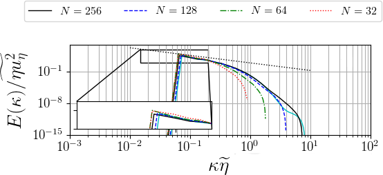
Figure 23: Energy spectra of forced turbulence simulations. The thin dotted line is at a $-5/3$ slope. The case $N=256$ with no-limiter is shown as a solid cyan line.

Additional inviscid simulations with the same forcing and initial conditions are performed to quantify the impact of viscosity and resolution. Figure 24 shows the original forced cases and $\mathrm{Re}=\infty$ cases at grid resolutions of $N=128$ and $64$. A forced turbulence DNS cases from Ref.  Rosales and Meneveau (2005) and explicit LES cases with $N=64$ and $N=128$ from Ref. Piomelli et al. (2015) with a similar linear forcing in physical space are included for comparison. Note that the forcing scheme used in the DNS and explicit SGS cases are performed with the velocity-pressure formulation using the velocity variable while the forcing in physical space employed in the present study uses the vorticity-velocity formulation on the vorticity variable. This may cause parameters selected in the forcing to behave with slight differences between the formulations. However, the spectra reveal that the low wavenumbers are relatively unaffected by the dissipation regardless of the Reynolds number and resolution. The impact of viscosity is seen in the high wavenumber scales. Furthermore, the forced ILES simulations show similar behaviors and trends to the DNS and explicit SGS in the low wavenumber region. The finite Reynolds number does have a larger impact on the inertial range compared to the DNS. At high Re, there is evidence of asymptotic convergence of flow statistics.

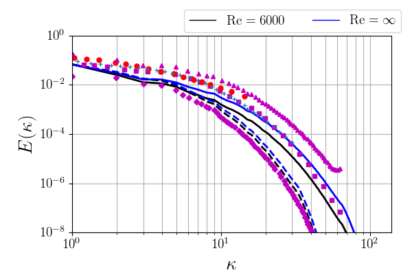
Figure 24: Energy spectra of forced turbulence simulations at $\mathrm{Re}=6000$ and $\mathrm{Re}=\infty$. The solid line is $N=128$ and the dashed line is $N=64$. The diamond, square, and triangle markers are forced turbulence cases 1, 2, and 3, respectively, from Ref. Rosales and Meneveau (2005). Circle and plus markers denote $N=64$ and $N=128$, respectively, and correspond to explicit LES of case 2 from Ref. Piomelli et al. (2015).

V.3 Temporally Evolving Jet

A temporally evolving jet provides a more rigorous test case where both large-scale features (Kelvin-Helmholtz instability) and small-scale fully-developed turbulence are presence. This is a flow that more closely resembles the complex flows with dominant coherent structures that the present scheme is designed to investigate.
The initial velocity flow field from Ref. da Silva and Pereira (2004) is given as follows:

$$u_{1}(\bm{x})=\frac{1}{2}-\frac{1}{2}\tanh\left[\frac{H}{4\theta_{0}}\left(1-\frac{2|x_{2}|}{H}\right)\right]$$ (46)

where $H$ is the initial jet thickness and $\theta_{0}$ is the initial momentum thickness. A $H/\theta_{0}=35$ is selected with a $\textrm{Re}=(U_{1}-U_{2})H/\nu=3200$. The initial $U_{1}=1$ and $U_{2}=0$. Initial velocity fluctuations are prescribed from the spectrum $E(k)\sim k^{4}\exp\left[-2(k/k_{0})^{2}\right]$. However, for the present scheme in the vorticity-velocity formulation we impose the initial condition based on the transverse vorticity as follows:

$$\omega_{3}(\bm{x})=\frac{1}{4\theta_{0}}\frac{|x_{2}|}{x_{2}}\cosh^{-2}\left[\frac{H}{4\theta_{0}}\left(1-\frac{2|x_{2}|}{H}\right)\right].$$ (47)

The initial condition has been shown to be a good estimate of the inlet velocity profile of spatially evolving jets. However, the temporally evolving jet provides a computationally expedient solution compared to simulating the spatial jet. The temporally evolving jet employs periodic boundary conditions on all sides of a cubic domain of $(L_{1}\times L_{2}\times L_{3})=(4H\times 4H\times 4H)$. Several grid resolution are used for comparison of the effects of the discretization: $N=64,128,$ and $256$, where $N$ is the number of grid cells per dimension. At $N=256$, the grid resolution is sufficiently fine to approach a DNS solution similar to the DNS simulation in Ref. da Silva and Pereira (2008). Both a dissipative ENO slope limiter and no-limiter are employed. The ENO slope limiter is similar to the minmod slope limiter but is not total variation diminishing. Contours of the out-of-plane vorticity are shown for each simulation in Fig. 25 at the time when the flow field becomes starts to become self-similar, $t/T_{ref}=15$, where $T_{ref}=H/\Delta U$, (see Fig. 26(a)). This time is equivalent to $x/H=7.5$ at the same Re for a spatially evolving jet. The three different grid resolutions demonstrate how different levels of resolution can affect features in the flow field. Each case using the ENO limiter show qualitatively the capture of large-scale coherent vortices, while the large-scale structure is less evident with the no-limiter case with low grid resolutions ($N=64$ and $128$).

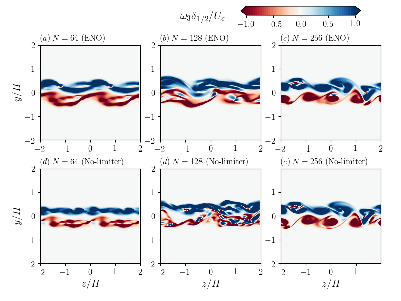
Figure 25: Velocity $\omega_{3}$ normalized by the jet half-width $\delta_{1/2}$ and centerline velocity for the temporally evolving jet contours for the temporally evolving jet at $t/T_{ref}=15$.

Figure 26(a) shows profiles of the mean streamwise velocity $\langle u_{1}\rangle$ in $x_{2}$ direction averaged over the $x_{1}$ and $x_{3}$ directions for each grid resolution and both the ENO limiter and no-limiter. The profiles are normalized by the centerline velocity $U_{c}=\langle u_{1}\rangle(x_{2}=0)$, while the jet half-width $\delta_{1/2}$, which is calculated with the mean streamwise velocity $\langle u_{1}\rangle(x_{2}=\delta_{1/2})-U_{\infty}=\frac{1}{2}\left(U_{c}-U_{\infty}\right)$ and $U_{\infty}$ is the streamwise velocity far from the jet, is used to normalize the abscissa. The profiles are chosen in the regime where the jet wake becomes self-similar. The grid resolution has a large effect on the amount of time the temporally evolving jet requires to become self-similar and will be discussed below. The streamwise velocity profiles are compared with several experimental measurements of spatial evolving jet in the self-similar regime. The present simulation results compare well with experimental measurements and show consistency between the different grid resolutions. Moreover, the spread in the results are comparable to DNS of temporal jets performed in Refs. da Silva and Pereira (2004, 2008). This suggests that even the low grid resolution of $N=64$ with the ENO limiter can capture some of the large-scale features well. The mean transverse vorticity profiles are shown in Fig. 26(b) for each simulation in the self-similar regime. The profiles indicate the mean vorticity from each simulation is captured reasonably well except the $N=64$ with the no-limiter case. However, the $N=64$ with dissipative ENO limiter, where the shear layer is only discretized by less than four grid cells, is captured reasonably. On the other hand, the $N=64$ and $128$ with no-limiter show slightly higher mean vorticity in the shear layer suggesting that under-resolved simulations need additional dissipation.

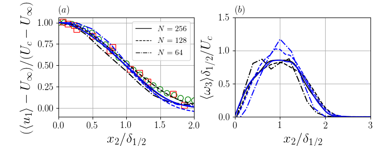
Figure 26: Profiles of the (a) mean streamwise velocity $\langle u_{1}\rangle$ normalized by the centerline velocity $U_{c}$ compared with experimental results from Ref. Gutmark and Wygnanski (1976) (circles) and Ref. Ramaprian and Chandrasekhara (1985) (squares) and (b) mean vorticity $\langle\omega_{3}\rangle$ normalized by the jet half-width $\delta_{1/2}$ and centerline velocity for the temporally evolving jet. Blue - no-limiter, Black - ENO limiter.

The second-order velocity statistics are compared with experimental measurements in Fig. 27. The rms (root-mean-square) streamwise velocity $\langle u^{2}_{1}\rangle^{1/2}$ profiles, shown in Fig. 27(a), and rms normal velocity $\langle u^{2}_{2}\rangle^{1/2}$ profiles, shown in Fig. 27(b), are compared with experimental measurements in the self-similar regime. While there are some differences between the different test cases, the overall comparison is reasonably well, especially for the lowest grid resolution case with the dissipative ENO limiter, which approximates sufficient dissipation. On the other hand, the lowest resolution with the no-limiter significantly under predicts the rms velocities. While scatter in the data can also be attributed to the relatively low number of samples for the temporally evolving jet especially at the lowest grid resolution, the role of numerical dissipation to capture flow statistics is apparent in the jet.

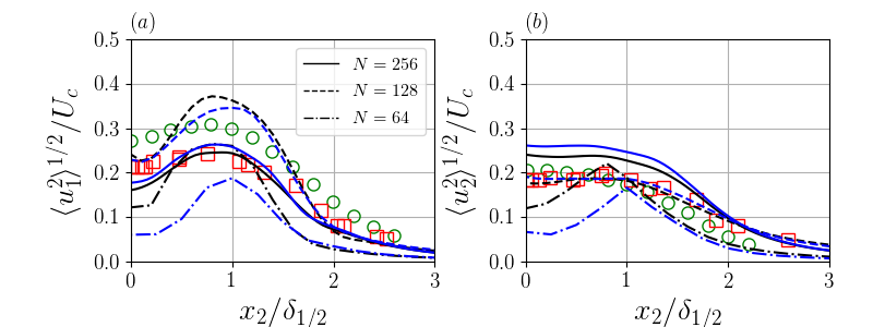
Figure 27: Profiles of the (a) rms (root-mean-square) streamwise velocity $\langle u^{2}_{1}\rangle^{1/2}$ and (b) rms normal velocity $\langle u^{2}_{2}\rangle^{1/2}$ normalized by the centerline velocity $U_{c}$ compared with experimental results from Ref. Gutmark and Wygnanski (1976) (circles) and Ref. Ramaprian and Chandrasekhara (1985) (squares). Blue - no-limiter, Black - ENO limiter.

The grid resolution and numerical dissipation affect the temporal evolution of the jet from its initial condition through the transition to turbulence. Up to this point, the result from the simulations have focused on the flow field after the jet transitions to turbulence, the transient behavior diminishes, and a self-similar regime occurs. In temporal jet simulations da Silva and Pereira (2008), the self-similar regime is obtained at times $t/T_{ref}>20$ for a similar initialization. This is equivalent to $x/H=10$ for a spatial-evolving jet. Figure 28 shows the evolution of the mean transverse vorticity profiles with time for each grid resolution case with the dissipative ENO limiter. The initial mean vorticity profile across the shear layer is relatively high and sharp. At further instances in time, the vorticity magnitude diminishes to a self-similar solution. Each grid resolution test case due to the increase numerical dissipation and grid cell size, transitions to the self-similar solution at different times. For the most resolve case, the self-similar solution is obtained at $t/T_{ref}>20$, while the lowest grid resolution transitions quicker, around $t/T_{ref}>10$. We are effectively solving the flow field at different effective Reynolds numbers through the transition to turbulence but are able to obtain a self-similar solution after the transition. The temporal impact of the numerical scheme on the flow field and the effective Reynolds number is significant when solving temporally evolving flows.

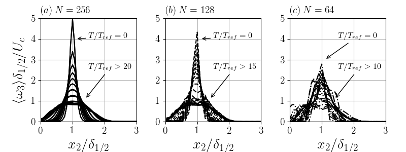
Figure 28: Temporal evolution of the vorticity profiles $\langle\omega_{3}\rangle$ for (a) $N=256$, (b) $N=128$ and (c) $N=64$. Each case employs the ENO limiter.

An estimate of the effective Reynolds number is determined from measurable features of the flow field. It is important to determine the effective Re to determine what the simulation is solving and if it has reached a minimum state in the sense of the asymptotic turbulence statistics. Here, we assume a high Reynolds number is achieved and using the asymptotic relationship for high Re regime of isotropic turbulence Kaneda et al. (2003) where $D=\epsilon L/U^{3}\approx\frac{1}{2}$ similar to ILES estimates for complex Richtmyer-Meshkov instabilities Zhou et al. (2014). The velocity scale $U=u^{\prime}=\langle(\frac{1}{3}u_{i}u_{i})^{1/2}\rangle$ and length scale $L$ is chosen to the jet half-width, which is shown as a function of the time in Fig. 29(a). The temporal evolution of the half-width shows that the grid resolution affects the jet spreading, which is expected based Fig. 28. The dissipation is obtained $\epsilon=DU^{3}/\delta_{1/2}$ and the effective viscosity is obtain through $\nu_{f}=\epsilon/\omega_{i}\omega_{i}$. Figure 29(b) shows the temporal evolution of the effective viscosity. For each grid resolution and slope limiter case, the initial effective viscosity behaves slightly differently, however, as the jet flow field asymptotically approaches the self-similar solution, the effective viscosity for each simulation approaches a single viscosity, which is the viscosity of the simulation. The numerical dissipation in the lowest resolution case is able to reach a state such that the asymptotic relationships in the jet can be reached. The $\textrm{Re}_{f}=u^{\prime}\delta_{1/2}/\nu_{f}$ is shown in Fig. 29(c). It indicates that the lower grid resolution cases with the increased dissipation are in fact solving a slightly different temporally evolving jet problem. However, because the flow comes self-similar at long times, this is not readily noticeable from profiles. Moreover, experimentation, both numerical and measurement, have shown that at high enough Re based on the inlet velocity and slot width (6000 and Ref. Klein et al. (2003) and 1000 in Ref. Deo et al. (2008), respectively) the spatially evolving planar jet becomes independent of Re, which comparable to the same Re for the present simulations ($Re\approx 3200$).

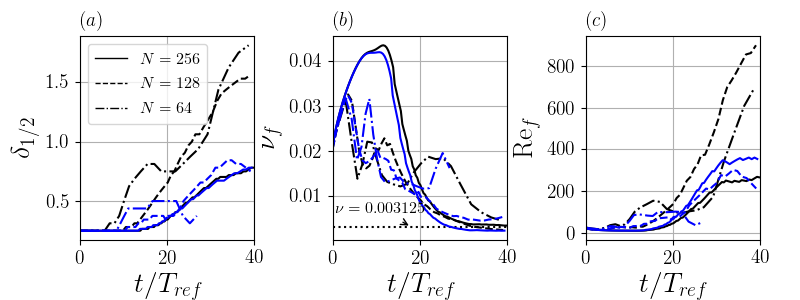
Figure 29: The temporal evolution of the (a) jet half-width, (b) effective viscosity, and (c) effective Re. Blue - no-limiter, Black - ENO limiter.

Energy spectra of the jet cases are shown in Fig. 30(a) for $N=256,128$ and $64$ for both the limited and no-limiter cases at $t/T_{ref}=40$. The spectra for the nearly resolved $N=256$ cases are comparatively similar. Furthermore, the $N=128$ case with the ENO limiter matches reasonably well in the large-scales but is slightly more dissipative than the $N=256$ cases in the high wavenumber range as expected. The lack of a limiter in the $N=128$ case shows that a non-dissipative scheme can have a large effect on the low wavenumbers. The lowest resolved cases, $N=64$ show some differences in the low wavenumbers. Additional Reynolds number cases are performed to assess the low wave number behavior and corroborate the results above that indicate the lower grid resolution are solving a slightly different temporally evolving jet problem. Figure 30(b) shows the $N=128$ resolution for $\mathrm{Re}=3200,1\times 10^{4},2\times 10^{5},$ and $\infty$. The higher Re numbers cases have an asymptotic behavior in the low wavenumbers which converge to the nearly resolved $N=256$ resolution. Additionally, this behavior is also found in the $N=64$ cases with high Re shown in Fig. 30(c). The viscosity $\mathrm{Re}=3200$ plays a significant role in dissipation but can be mitigate by carefully selecting the grid resolution. The spectra show that with adequate resolution and a high enough Re, the solution converges to correct results especially in the low wavenumber range, which is most important for performing LES. The estimation of an effective Re becomes especially critical when attempting ILES of more complex flow fields where the flow characteristics can become independent of Re such as wind turbine wakes Chamorro et al. (2012). By selecting the grid resolution for the problem, an ILES with the present scheme can be employed such that the large-scale structures are captured and small-scale turbulence are implicitly modeled to obtain physically accurate, expedient results.

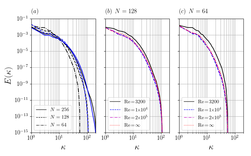
Figure 30: Energy spectra $E(k)$ of simulations temporal simulations: (a) $\mathrm{Re}=3200$ at several discretizations, Blue - no-limiter, Black - ENO limiter, (b) $N=128$ case at different $\mathrm{Re}$, and (c) $N=64$ case at different $\mathrm{Re}$.

VI Conclusions

The subgrid scale characteristics and effectiveness of an upwind finite volume scheme for the vorticity transport equations were investigated. The numerical scheme employs a generalized Riemann problem-based multi-dimensional wave propagation approach. Modified equation analysis was used to characterize the dissipation and backscatter. The analysis revealed two limits for including dissipation implicitly through numerics: 1.) a low dissipation limit using a second-order central difference, most appropriate in smooth areas, i.e. regions dominated by large vortical coherent structures; and 2.) a high dissipation limit using a first order upwind difference, used when the vorticity changes rapidly across grid cells, i.e., regions of under-resolved turbulence. While the former is ideal in well-resolved areas of the flow field, the latter is necessary in regions in which dissipation is essential to account for the transfer of energy from the resolved scales to the sub-grid scales in the absence of an explicit SGS model. The modified equation at the high dissipation limit contains many terms, some of which can be combined into forms that are similar to commonly used explicit sub-grid scale models including the tensor-gradient models, hyper-viscosity model, and a simple gradient model. This serves a qualitative tool to understand the implications of using the present scheme for ILES. We are careful to note that—for ILES in general—the terms in the modified equation do not have to be similar to explicit SGS terms. Rather, the similarities to known models provide insight in characterizing the scheme.
To characterize turbulence with the present scheme for the ILES methodology, a series of turbulence-in-a-box simulations of the Taylor-Green vortex was performed to understand the process of energy transfer from energy-containing scales to the sub-grid scale. The Taylor-Green vortex cases revealed that the grid resolution must be carefully taken into account in order to obtain desired results. The grid resolution is the largest factor for the magnitude of the effective Re while the choice of limiter, which subtly controls the numerical dissipation, has an impact on the accuracy. However, in under-resolved simulations, a dissipative limiter is essential. The dissipation terms obtained from the modified equation analysis are shown to faithfully represent the implicit SGS torque in the Taylor-Green vortex case. In high Reynolds number flows, where there is a marked separation of scales, the method is able to represent the high energy modes. Further numerical experiments with forced turbulence revealed that high-Reynolds number asymptotic turbulence statistics can be reasonably captured with the ILES methodology for this vorticity-velocity formulation scheme.
Finally, simulations of a temporally evolving jet, which contains both large-scale vortical structures and fine-scale turbulence show that under-resolved numerics can capture asymptotic turbulence statistics and large-scale features. The method is particularly useful when the effective Reynolds number is past a threshold beyond which the flow is dependent on the Reynolds number.

The simulations studied herein represent canonical flows which allow us to build our understanding of the method to more complex flows. The simulation tests show that coarse grid resolutions provide a good estimate for large energy-containing modes given a large enough inertial range. This particular vorticity-velocity scheme was designed to capture and preserve large vorticity structures in flows in which fully-developed small-scale turbulence tends to localized and large energy-containing structures dominate the flow. Our previous work Foti and Duraisamy (2018) showed how the scheme can be used to capture vortical structures, while this work indicates that the impact of fine-scale turbulence on the energy-containing scales can also be reasonably represented.

References

- Yule (1978) AJ Yule, “Large-scale structure in the mixing layer of a round jet,” Journal of Fluid Mechanics 89, 413–432 (1978).
- Akselvoll and Moin (1996) Knut Akselvoll and Parviz Moin, “Large-eddy simulation of turbulent confined coannular jets,” Journal of Fluid Mechanics 315, 387–411 (1996).
- Foti et al. (2016) Daniel Foti, Xiaolei Yang, Michele Guala, and Fotis Sotiropoulos, “Wake meandering statistics of a model wind turbine: Insights gained by large eddy simulations,” Physical Review Fluids 1, 044407 (2016).
- Foti et al. (2018) Daniel Foti, Xiaolei Yang, Filippo Campagnolo, David Maniaci, and Fotis Sotiropoulos, “Wake meandering of a model wind turbine operating in two different regimes,” Physical Review Fluids 3, 054607 (2018).
- Guala et al. (2011) Michele Guala, M Metzger, and Beverley J McKeon, “Interactions within the turbulent boundary layer at high reynolds number,” Journal of Fluid Mechanics 666, 573–604 (2011).
- Fang and Porté-Agel (2015) Jiannong Fang and Fernando Porté-Agel, “Large-eddy simulation of very-large-scale motions in the neutrally stratified atmospheric boundary layer,” Boundary-Layer Meteorology 155, 397–416 (2015).
- Kravchenko and Moin (1997) AG Kravchenko and Parviz Moin, “On the effect of numerical errors in large eddy simulations of turbulent flows,” Journal of Computational Physics 131, 310–322 (1997).
- Chow and Moin (2003) Fotini Katopodes Chow and Parviz Moin, “A further study of numerical errors in large-eddy simulations,” Journal of Computational Physics 184, 366–380 (2003).
- Freitag and Klein (2006) Martin Freitag and Markus Klein, “An improved method to assess the quality of large eddy simulations in the context of implicit filtering,” Journal of Turbulence , N40 (2006).
- Toosi and Larsson (2020) Siavash Toosi and Johan Larsson, “Towards systematic grid selection in LES: Identifying the optimal spatial resolution by minimizing the solution sensitivity,” Computers & Fluids , 104488 (2020).
- Smagorinsky (1963) Joseph Smagorinsky, “General circulation experiments with the primitive equations: I. The basic experiment,” Monthly Weather Review 91, 99–164 (1963).
- Germano et al. (1991) Massimo Germano, Ugo Piomelli, Parviz Moin, and William H Cabot, “A dynamic subgrid-scale eddy viscosity model,” Physics of Fluids A: Fluid Dynamics 3, 1760–1765 (1991).
- Bardina et al. (1980) Jorge Bardina, J Ferziger, and WC Reynolds, “Improved subgrid-scale models for large-eddy simulation,” in 13th Fluid and Plasma Dynamics Conference (1980) p. 1357.
- Lilly (1992) Douglas K Lilly, “A proposed modification of the Germano subgrid-scale closure method,” Physics of Fluids A: Fluid Dynamics 4, 633–635 (1992).
- Clark et al. (1979) Robert A Clark, Joel H Ferziger, and William Craig Reynolds, “Evaluation of subgrid-scale models using an accurately simulated turbulent flow,” Journal of Fluid Mechanics 91, 1–16 (1979).
- Bou-Zeid et al. (2005) Elie Bou-Zeid, Charles Meneveau, and Marc Parlange, “A scale-dependent Lagrangian dynamic model for large eddy simulation of complex turbulent flows,” Physics of Fluids 17, 025105 (2005).
- Yu et al. (2017) Changping Yu, Zuoli Xiao, and Xinliang Li, “Scale-adaptive subgrid-scale modelling for large-eddy simulation of turbulent flows,” Physics of Fluids 29, 035101 (2017).
- Chapelier et al. (2018) J-B Chapelier, Bono Wasistho, and Carlo Scalo, “A coherent vorticity preserving eddy-viscosity correction for large-eddy simulation,” Journal of Computational Physics 359, 164–182 (2018).
- Schneider et al. (2005) Kai Schneider, Marie Farge, Giulio Pellegrino, and Michael M Rogers, “Coherent vortex simulation of three-dimensional turbulent mixing layers using orthogonal wavelets,” Journal of Fluid Mechanics 534, 39 (2005).
- Ouvrard et al. (2010) Hilde Ouvrard, Bruno Koobus, Alain Dervieux, and Maria Vittoria Salvetti, “Classical and variational multiscale LES of the flow around a circular cylinder on unstructured grids,” Computers & Fluids 39, 1083–1094 (2010).
- Parish and Duraisamy (2017a) Eric J Parish and Karthik Duraisamy, “A dynamic subgrid scale model for large eddy simulations based on the Mori–Zwanzig formalism,” Journal of Computational Physics 349, 154–175 (2017a).
- Parish and Duraisamy (2017b) Eric J Parish and Karthik Duraisamy, “Non-Markovian closure models for large eddy simulations using the Mori-Zwanzig formalism,” Physical Review Fluids 2, 014604 (2017b).
- Geurts (1997) Bernard J Geurts, “Inverse modeling for large-eddy simulation,” Physics of Fluids 9, 3585–3587 (1997).
- Zhou et al. (2018) Zhideng Zhou, Shizhao Wang, and Guodong Jin, “A structural subgrid-scale model for relative dispersion in large-eddy simulation of isotropic turbulent flows by coupling kinematic simulation with approximate deconvolution method,” Physics of Fluids 30, 105110 (2018).
- Kraichnan (1970) Robert H Kraichnan, “Diffusion by a random velocity field,” Physics of Fluids 13, 22–31 (1970).
- Boris et al. (1992) JP Boris, FF Grinstein, ES Oran, and RL Kolbe, “New insights into large eddy simulation,” Fluid Dynamics Research 10, 199–228 (1992).
- Youngs (1991) David L Youngs, “Three-dimensional numerical simulation of turbulent mixing by Rayleigh–Taylor instability,” Physics of Fluids A: Fluid Dynamics 3, 1312–1320 (1991).
- Gathmann et al. (1993) Ralf Jens Gathmann, Mohammed Si-Ameur, and Fabrice Mathey, “Numerical simulations of three-dimensional natural transition in the compressible confined shear layer,” Physics of Fluids A: Fluid Dynamics 5, 2946–2968 (1993).
- Smolarkiewicz and Margolin (1998) Piotr K Smolarkiewicz and Len G Margolin, “MPDATA: A finite-difference solver for geophysical flows,” Journal of Computational Physics 140, 459–480 (1998).
- Thornber et al. (2007) Ben Thornber, Andrew Mosedale, and Dimitris Drikakis, “On the implicit large eddy simulations of homogeneous decaying turbulence,” Journal of Computational Physics 226, 1902–1929 (2007).
- Wachtor et al. (2013) Adam J Wachtor, Fernando F Grinstein, Carl R DeVore, JR Ristorcelli, and Len G Margolin, “Implicit large-eddy simulation of passive scalar mixing in statistically stationary isotropic turbulence,” Physics of Fluids 25, 025101 (2013).
- Margolin and Rider (2002) Len G Margolin and William J Rider, “A rationale for implicit turbulence modelling,” International Journal for Numerical Methods in Fluids 39, 821–841 (2002).
- Margolin and Rider (2005) LG Margolin and WJ Rider, “The design and construction of implicit LES models,” International Journal for Numerical Methods in Fluids 47, 1173–1179 (2005).
- Margolin et al. (2006) LG Margolin, WJ Rider, and FF Grinstein, “Modeling turbulent flow with implicit LES,” Journal of Turbulence , N15 (2006).
- Drikakis et al. (2009) Dimitris Drikakis, Marco Hahn, Andrew Mosedale, and Ben Thornber, “Large eddy simulation using high-resolution and high-order methods,” Philosophical Transactions of the Royal Society A: Mathematical, Physical and Engineering Sciences 367, 2985–2997 (2009).
- Zhou et al. (2014) Ye Zhou, Fernando F Grinstein, Adam J Wachtor, and Brian M Haines, “Estimating the effective Reynolds number in implicit large-eddy simulation,” Physical Review E 89, 013303 (2014).
- Hickel et al. (2006) Stefan Hickel, Nikolaus A Adams, and J Andrzej Domaradzki, “An adaptive local deconvolution method for implicit LES,” Journal of Computational Physics 213, 413–436 (2006).
- Margolin et al. (1999) Len G Margolin, Piotr K Smolarkiewicz, and Zbigniew Sorbjan, “Large-eddy simulations of convective boundary layers using nonoscillatory differencing,” Physica D: Nonlinear Phenomena 133, 390–397 (1999).
- Fureby and Grinstein (2002) Christer Fureby and Fernando F Grinstein, “Large eddy simulation of high-Reynolds-number free and wall-bounded flows,” Journal of Computational Physics 181, 68–97 (2002).
- Grinstein and Fureby (2007) Fernando F Grinstein and Christer Fureby, “On flux-limiting-based implicit large eddy simulation,” Journal of Fluids Engineering 129, 1483–1492 (2007).
- Hussain (1986) AKM Fazle Hussain, “Coherent structures and turbulence,” Journal of Fluid Mechanics 173, 303–356 (1986).
- Papamoschou and Lele (1993) Dimitri Papamoschou and Sanjiva K Lele, “Vortex-induced disturbance field in a compressible shear layer,” Physics of Fluids A: Fluid Dynamics 5, 1412–1419 (1993).
- Duraisamy and Lele (2008) Karthik Duraisamy and Sanjiva K Lele, “Evolution of isolated turbulent trailing vortices,” Physics of Fluids 20, 035102 (2008).
- Koumoutsakos and Leonard (1995) Petros Koumoutsakos and A Leonard, “High-resolution simulations of the flow around an impulsively started cylinder using vortex methods,” Journal of Fluid Mechanics 296, 1–38 (1995).
- Foti and Duraisamy (2018) Daniel Foti and Karthik Duraisamy, “Multi-dimensional finite volume scheme for the vorticity transport equations,” Computers & Fluids 167, 17–32 (2018).
- Brown and Line (2005) Richard E Brown and Andrew J Line, “Efficient high-resolution wake modeling using the vorticity transport equation,” AIAA Journal 43, 1434–1443 (2005).
- Whitehouse and Boschitsch (2014) Glen R Whitehouse and Alexander H Boschitsch, “Innovative grid-based vorticity–velocity solver for analysis of vorticity-dominated flows,” AIAA Journal 53, 1655–1669 (2014).
- Koumoutsakos (2005) Petros Koumoutsakos, “Multiscale flow simulations using particles,” Annu. Rev. Fluid Mech. 37, 457–487 (2005).
- Winckelmans et al. (1996) Grégoire Winckelmans, TS Lund, Daniele Carati, and AA Wray, “A priori testing of subgrid-scale models for the velocity-pressure and vorticity-velocity formulations,” in Proceedings of the CTR Summer Program (1996) p. 309.
- Cottet (1990) Georges-Henri Cottet, “A particle-grid superposition method for the Navier-Stokes equations,” Journal of Computational Physics 89, 301–318 (1990).
- Ould-Salihi et al. (2001) Mohamed Lemine Ould-Salihi, Georges-Henri Cottet, and Mohammed El Hamraoui, “Blending finite-difference and vortex methods for incompressible flow computations,” SIAM Journal on Scientific Computing 22, 1655–1674 (2001).
- Rennich and Lele (1997) Steven C Rennich and Sanjiva K Lele, “Numerical method for incompressible vortical flows with two unbounded directions,” Journal of computational physics 137, 101–129 (1997).
- Zhao and He (2011) J Zhao and C He, “A hybrid solver with combined CFD and viscous vortex particle method,” in 67th Annual Forum of the American Helicopter Society (2011).
- Stone et al. (2010) Christopher Stone, Earl Duque, Christopher Hennes, and Adrin Gharakhani, “Rotor wake modeling with a coupled Eulerian and vortex particle method,” in 48th AIAA Aerospace Sciences Meeting (2010) pp. 2010–0312.
- Mansfield et al. (1998) John R Mansfield, Omar M Knio, and Charles Meneveau, “A dynamic LES scheme for the vorticity transport equation: Formulation and a priori tests,” Journal of Computational Physics 145, 693–730 (1998).
- Meitz and Fasel (2000) Hubert L Meitz and Hermann F Fasel, “A compact-difference scheme for the Navier–Stokes equations in vorticity–velocity formulation,” Journal of Computational Physics 157, 371–403 (2000).
- Davies and Carpenter (2001) Christopher Davies and Peter W Carpenter, “A novel velocity–vorticity formulation of the Navier–Stokes equations with applications to boundary layer disturbance evolution,” Journal of Computational Physics 172, 119–165 (2001).
- Parish et al. (2016) Eric Parish, Karthik Duraisamy, and Praveen Chandrashekar, “Generalized Riemann problem-based upwind scheme for the vorticity transport equations,” Computers & Fluids 132, 10–18 (2016).
- Chamorro et al. (2012) Leonardo P Chamorro, REA Arndt, and F Sotiropoulos, “Reynolds number dependence of turbulence statistics in the wake of wind turbines,” Wind Energy 15, 733–742 (2012).
- Godunov (1972) SK Godunov, “Symmetric form of the equations of magnetohydrodynamics,” Numerical Methods for Mechanics of Continuum Medium 1, 26–34 (1972).
- Powell (1997) Kenneth G Powell, “An approximate Riemann solver for magnetohydrodynamics,” in Upwind and High-Resolution Schemes (Springer, 1997) pp. 570–583.
- Bale et al. (2003) Derek S Bale, Randall J LeVeque, Sorin Mitran, and James A Rossmanith, “A wave propagation method for conservation laws and balance laws with spatially varying flux functions,” SIAM Journal on Scientific Computing 24, 955–978 (2003).
- LeVeque (1996) Randall J LeVeque, “High-resolution conservative algorithms for advection in incompressible flow,” SIAM Journal on Numerical Analysis 33, 627–665 (1996).
- Hirt (1968) Cyril W Hirt, “Heuristic stability theory for finite-difference equations,” Journal of Computational Physics 2, 339–355 (1968).
- Borue and Orszag (1998) Vadim Borue and Steven A Orszag, “Local energy flux and subgrid-scale statistics in three-dimensional turbulence,” Journal of Fluid Mechanics 366, 1–31 (1998).
- Vreman et al. (1996) Bert Vreman, Bernard Geurts, and Hans Kuerten, “Large-eddy simulation of the temporal mixing layer using the Clark model,” Theoretical and Computational Fluid Dynamics 8, 309–324 (1996).
- Cerutti et al. (2000) Stefano Cerutti, Charles Meneveau, and Omar M Knio, “Spectral and hyper eddy viscosity in high-Reynolds-number turbulence,” Journal of Fluid Mechanics 421, 307–338 (2000).
- Lamorgese et al. (2005) AG Lamorgese, DA Caughey, and SB Pope, “Direct numerical simulation of homogeneous turbulence with hyperviscosity,” Physics of Fluids 17, 015106 (2005).
- Frisch (1995) Uriel Frisch, Turbulence: the legacy of AN Kolmogorov (Cambridge University Press, 1995).
- Brachet (1991) ME Brachet, “Direct simulation of three-dimensional turbulence in the Taylor–Green vortex,” Fluid Dynamics Research 8, 1–8 (1991).
- Brachet et al. (1983) Marc E Brachet, Daniel I Meiron, Steven A Orszag, BG Nickel, Rudolf H Morf, and Uriel Frisch, “Small-scale structure of the Taylor–Green vortex,” Journal of Fluid Mechanics 130, 411–452 (1983).
- Drikakis et al. (2007) Dimitris Drikakis, Christer Fureby, Fernando F Grinstein, and David Youngs, “Simulation of transition and turbulence decay in the Taylor–Green vortex,” Journal of Turbulence , N20 (2007).
- Grinstein et al. (2011) FF Grinstein, AA Gowardhan, and AJ Wachtor, “Simulations of Richtmyer–Meshkov instabilities in planar shock-tube experiments,” Physics of Fluids 23, 034106 (2011).
- da Silva and Pereira (2004) Carlos B da Silva and José CF Pereira, “The effect of subgrid-scale models on the vortices computed from large-eddy simulations,” Physics of Fluids 16, 4506–4534 (2004).
- Zhou et al. (2020) Ye Zhou, Michael Groom, and Ben Thornber, “Dependence of enstrophy transport and mixed mass on dimensionality and initial conditions in the richtmyer–meshkov instability induced flows,” Journal of Fluids Engineering 142 (2020).
- Zhou and Thornber (2016) Ye Zhou and Ben Thornber, “A comparison of three approaches to compute the effective Reynolds number of the implicit large-eddy simulations,” Journal of Fluids Engineering 138 (2016).
- Kaneda et al. (2003) Yukio Kaneda, Takashi Ishihara, Mitsuo Yokokawa, Ken’ichi Itakura, and Atsuya Uno, “Energy dissipation rate and energy spectrum in high resolution direct numerical simulations of turbulence in a periodic box,” Physics of Fluids 15, L21–L24 (2003).
- Falkovich (1994) Gregory Falkovich, “Bottleneck phenomenon in developed turbulence,” Physics of Fluids 6, 1411–1414 (1994).
- Wang et al. (1996) Lian-Ping Wang, Shiyi Chen, James G Brasseur, and John C Wyngaard, “Examination of hypotheses in the Kolmogorov refined turbulence theory through high-resolution simulations. Part 1. Velocity field,” Journal of Fluid Mechanics 309, 113–156 (1996).
- Sreenivasan (1998) Katepalli R Sreenivasan, “An update on the energy dissipation rate in isotropic turbulence,” Physics of Fluids 10, 528–529 (1998).
- Zhou (2007) Ye Zhou, “Unification and extension of the similarity scaling criteria and mixing transition for studying astrophysics using high energy density laboratory experiments or numerical simulations,” Physics of Plasmas 14, 082701 (2007).
- Sreenivasan (1984) Katepalli R Sreenivasan, “On the scaling of the turbulence energy dissipation rate,” Physics of Fluids 27, 1048–1051 (1984).
- Dimotakis (2000) Paul E Dimotakis, “The mixing transition in turbulent flows,” Journal of Fluid Mechanics 409, 69–98 (2000).
- Tennekes and Lumley (1972) Hendrik Tennekes and John Leask Lumley, A first course in turbulence (MIT press, 1972).
- Sagaut and Cambon (2008) Pierre Sagaut and Claude Cambon, Homogeneous turbulence dynamics, Vol. 10 (Springer, 2008).
- Rosales and Meneveau (2005) Carlos Rosales and Charles Meneveau, “Linear forcing in numerical simulations of isotropic turbulence: Physical space implementations and convergence properties,” Physics of Fluids 17, 095106 (2005).
- Mansour and Wray (1994) NN Mansour and AA Wray, “Decay of isotropic turbulence at low Reynolds number,” Physics of Fluids 6, 808–814 (1994).
- Rogallo (1981) RS Rogallo, “Numerical experiments in homogeneous turbulence,” NASA STI/Recon Technical Report N 81 (1981).
- Jiménez et al. (1993) Javier Jiménez, Alan A Wray, Philip G Saffman, and Robert S Rogallo, “The structure of intense vorticity in isotropic turbulence,” Journal of Fluid Mechanics 255, 65–90 (1993).
- Castaing et al. (1990) B Castaing, Y Gagne, and EJ Hopfinger, “Velocity probability density functions of high Reynolds number turbulence,” Physica D: Nonlinear Phenomena 46, 177–200 (1990).
- Jimenez and Wray (1998) Javier Jimenez and Alan A Wray, “On the characteristics of vortex filaments in isotropic turbulence,” Journal of Fluid Mechanics 373, 255–285 (1998).
- Cantwell (1993) Brian J Cantwell, “On the behavior of velocity gradient tensor invariants in direct numerical simulations of turbulence,” Physics of Fluids A: Fluid Dynamics 5, 2008–2013 (1993).
- Piomelli et al. (2015) Ugo Piomelli, Amirreza Rouhi, and Bernard J Geurts, “A grid-independent length scale for large-eddy simulations,” Journal of fluid mechanics 766, 499 (2015).
- da Silva and Pereira (2008) Carlos B da Silva and José CF Pereira, “Invariants of the velocity-gradient, rate-of-strain, and rate-of-rotation tensors across the turbulent/nonturbulent interface in jets,” Physics of Fluids 20, 055101 (2008).
- Gutmark and Wygnanski (1976) E Gutmark and I Wygnanski, “The planar turbulent jet,” Journal of Fluid Mechanics 73, 465–495 (1976).
- Ramaprian and Chandrasekhara (1985) BR Ramaprian and MS Chandrasekhara, “LDA measurements in plane turbulent jets,” Journal of Fluids Engineering 107, 264–271 (1985).
- Klein et al. (2003) M Klein, A Sadiki, and J Janicka, “Investigation of the influence of the Reynolds number on a plane jet using direct numerical simulation,” International Journal of Heat and Fluid Flow 24, 785–794 (2003).
- Deo et al. (2008) Ravinesh C Deo, Jianchun Mi, and Graham J Nathan, “The influence of Reynolds number on a plane jet,” Physics of Fluids 20, 075108 (2008).