Memories of past close encounters in extreme trans-Neptunian space: Finding unseen planets using pure random searches

Abstract

Context. The paths followed by the known extreme trans-Neptunian objects (ETNOs) effectively avoid direct gravitational perturbations from the four giant planets, yet their orbital eccentricities are in the range between 0.69–0.97. Solar system dynamics studies show that such high values of the eccentricity can be produced via close encounters or secular perturbations. In both cases, the presence of yet-to-be-discovered trans-Plutonian planets is required. Recent observational evidence cannot exclude the existence, at 600 AU from the Sun, of a planet of five Earth masses.

Aims. If the high eccentricities of the known ETNOs are the result of relatively recent close encounters with putative planets, the mutual nodal distances of sizeable groups of ETNOs with their assumed perturber may still be small enough to be identifiable geometrically. In order to confirm or reject this possibility, we used Monte Carlo random search techniques.

Methods. Two arbitrary orbits may lead to close encounters when their mutual nodal distance is sufficiently small. We generated billions of random planetary orbits with parameters within the relevant ranges and computed the mutual nodal distances with a set of randomly generated orbits with parameters consistent with those of the known ETNOs and their uncertainties. We monitored which planetary orbits had the maximum number of potential close encounters with synthetic ETNOs and we studied the resulting distributions.

Results. We provide narrow ranges for the orbital parameters of putative planets that may have experienced orbit-changing encounters with known ETNOs. Some sections of the available orbital parameter space are strongly disfavored by our analysis.

Conclusions. Our calculations suggest that more than one perturber is required if scattering is the main source of orbital modification for the known ETNOs. Perturbers might not be located farther than 600 AU and they have to follow moderately eccentric and inclined orbits to be capable of experiencing close encounters with multiple known ETNOs.

1 Introduction

Extreme trans-Neptunian objects (ETNOs) serve as unique probes into the gravity perturbations shaping the outer solar system beyond the classical trans-Neptunian or Kuiper belt (see e.g., Kaib et al. 2019). The trajectories followed by the known ETNOs effectively avoid direct gravitational perturbations from the four giant planets, yet their orbital eccentricities are in the range 0.69–0.97. Efficient drivers for the eccentricity excitation of small bodies include close encounters with planets (see e.g., Carusi et al. 1990) and the von Zeipel-Lidov-Kozai mechanism (von Zeipel 1910; Kozai 1962; Lidov 1962; Ito & Ohtsuka 2019). In both cases above and in the case of ETNOs, the presence of yet-to-be-discovered trans-Plutonian planets is required.

Fienga et al. (2020) used the INPOP19a planetary ephemerides that include Jupiter-updated positions by the Juno mission and a reanalysis of Cassini observations to show that there is no clear evidence for the existence of the so-called Planet 9 predicted by Batygin & Brown (2016) as an explanation for the orbital architecture of the known ETNOs. However, Fienga et al. (2020) concluded that if Planet 9 exists, it cannot be closer than 500 AU, if it has a mass of 5 $M_{\oplus}$, and no closer than 650 AU, if it has a mass of 10 $M_{\oplus}$. The latest version of the Planet 9 hypothesis (Batygin et al. 2019) predicts the existence of a planet with a mass in the range 5–10 $M_{\oplus}$, following an orbit with a value of the semi-major axis in the range of 400–800 AU, eccentricity in the range of 0.2–0.5, and inclination in the interval between (15°, 25°). A number of exoplanets have already been observed orbiting at hundreds of AUs from their host stars (see e.g., Bailey et al. 2014; Naud et al. 2014; Nguyen et al. 2021) and theoretical calculations have confirmed plausible pathways for their formation (see e.g., Kenyon & Bromley 2015, 2016).

If the high eccentricities of known ETNOs are the result of relatively recent close encounters with putative planets, the mutual nodal distances of sizeable groups of ETNOs with their assumed perturber may still be small enough to be identifiable geometrically. Here, we use Monte Carlo random search techniques to identify orbits that may lead to the maximum number of potential close encounters with synthetic ETNOs whose orbital parameters are consistent with those of the real ETNOs and their uncertainties. This letter is organized as follows. In Sect. 2, we review our methodology and present the data used in our analyses. In Sect. 3, we apply our methodology and discuss its results. Our conclusions are summarized in Sect. 4.

2 Methods and data description

This work explores a ”what if” scenario in which the starting hypothesis states that a sizeable number of known ETNOs have experienced relatively recent close encounters with putative planets; the timescale comes constrained by their orbital periods that are in the range 1867–50116 yr, so encounters may have taken place during the last 10³–10⁵ yr. In this work, therefore, we are testing the hypothesis statistically. If this hypothesis is plausible, a statistically significant number of compatible planetary perturber orbits should emerge from the analysis of a very large sample of orbits. If the distributions of one or more of the orbital parameters of the candidate are flat, the starting hypothesis must be rejected as this would show that there is no favored orbital solution for the perturber; conversely, if all the distributions produce consistent intervals that are statistically significant, the plausibility of the starting hypothesis can be considered as confirmed. Plausibility concerns the likelihood of acceptance, not the likelihood of being true or better than competing scenarios. The problem under investigation here is equivalent to a nondifferenciable optimization that is well-suited for a uniform Monte Carlo random search (Metropolis & Ulam 1949). Our methodology brings together geometry and statistics in our attempt to find the confocal ellipse that passes the closest to the maximum number of known orbits of a certain dynamical class; this approach is fundamentally different from those involving $N$-body calculations and statistics (see e.g., de la Fuente Marcos et al. 2016; de León et al. 2017; de la Fuente Marcos et al. 2017). Kalinicheva & Chernetenko (2020) recently applied a geometric approach within the context of the Planet 9 hypothesis.

2.1 Methodology

Two arbitrary orbits may experience close encounters when their mutual nodal distance is sufficiently small. Recurrent (or even single) encounters within 1 Hill radius (Hamilton & Burns 1992) of a massive body may change the orbit of a small body significantly. The mutual nodal distance between the orbits of a small body (an ETNO in our case) and an arbitrary planet can be computed as described in Appendix A. Orbits are defined by the values of semi-major axis, $a$ (that controls size), eccentricity, $e$ (that controls shape), and those of the angular elements — inclination, $i$, longitude of the ascending node, $\Omega$, and argument of perihelion, $\omega$ — that control the orientation in space of the orbit; the perihelion distance or pericenter, $q$, is given by the expression $q=a\,(1-e)$. The actual position of an object in its orbit is controled by a fourth angle, the mean anomaly, $M$. Our geometric approach leaves this angle out of the analysis and, therefore, it is not capable of predicting the current location of the perturber, if it is, in fact, real.

We generated 2$\times$10¹⁰ random planetary orbits with uniformly distributed relevant parameters: $\Omega_{\rm p}$ and $\omega_{\rm p}$ $\in(0\degr,360\degr)$, $i_{\rm p}\in(0\degr,80\degr)$, $e_{\rm p}\in(0,0.9),$ and $q_{\rm p}\in(x,1000-x)$ AU, with $x=300,400,500,$ and 600 AU so $a_{\rm p}=q_{\rm p}/(1-e_{\rm p})$. For each random planetary orbit, we computed the mutual nodal distances between a set of synthetic ETNOs and the planet. Each set of synthetic ETNOs was generated using the mean values and standard deviations of the orbit determinations of the known ETNOs as pointed out in Appendix B.

For each combination of random planetary orbit and synthetic (but compatible with the observations) set of ETNOs, we have counted how many synthetic ETNOs had at least one mutual nodal distance with the planet under 5 AU (for $x=300$ AU), 7.5 AU (for $x=400$ AU), and 10 AU (for $x=500$ and 600 AU). We then proceeded to record the random planetary orbit if the count was $\geq 5$, in order to maximize the number of potential close approaches between planet and set of ETNOs. We then studied the resulting distributions. In order to analyze the results, we produced histograms using the Matplotlib library (Hunter 2007) with sets of bins computed using NumPy (van der Walt et al. 2011) by applying the Freedman and Diaconis rule (Freedman & Diaconis 1981). Instead of using frequency-based histograms, we considered counts to form a probability density so the area under the histogram will sum to one.

The nodal distance separation criteria for selective counting are not arbitrary but motivated by the results in Fienga et al. (2020), a 2 $M_{\oplus}$ has a Hill radius of 4.5 AU (if $a_{\rm p}=400$ AU and $e_{\rm p}=0.1$), a 5 $M_{\oplus}$ has a Hill radius of 9.2 AU (if $a_{\rm p}=542$ AU and $e_{\rm p}=0.01$). Therefore, we implicitly assume that the farther away the pericenter of the planet is, the more massive it may be.

2.2 Data sources

Here, we work with publicly available data from Jet Propulsion Laboratory’s (JPL) Small-Body Database (SBDB) and HORIZONS on-line solar system data and ephemeris computation service, both provided by the Solar System Dynamics Group (Giorgini 2015). Assuming the definition in Trujillo & Sheppard (2014), that the ETNOs have $q>30$ AU and $a>150$ AU, the sample of known ETNOs now includes 39 objects with reliable orbits (see Appendix B) whose data have been retrieved from JPL’s SBDB and HORIZONS using tools provided by the Python package Astroquery (Ginsburg et al. 2019). In the following section, we use barycentric elements because within the context of the ETNOs, barycentric orbit determinations better account for their changing nature as Jupiter follows its 12 yr orbit around the Sun; Appendix C shows results based on heliocentric orbits that are consistent with those of the barycentric ones.

3 Results and discussion

As pointed out above, the motivation behind this study is the belief that a fossil record of planetary encounters might be preserved in the distribution of the orbital elements of ETNOs. With this hypothesis in mind, we monitored which planetary orbits had the maximum number of potential close encounters with synthetic ETNOs and analyzed the resulting distributions that are shown in Fig. 1. The first (leftmost) column of panels shows the results based on the assumption that $q_{\rm p}>300$ AU, including 20304 orbits with a number of potential close approaches in the range between 5–7; the next one, shows results for $q_{\rm p}>400$ AU also with a range of potential close approaches of 5–7 for 5671 orbits; the following column of panels displays results for $q_{\rm p}>500$ AU with a range of 5–6 for 2635 orbits; the right column shows panels with results for $q_{\rm p}>600$ AU and the number of potential close approaches between planet and set of ETNOs is just 5 for 56 orbits. From these values and the plots, it is increasingly difficult to find consistent perturbers as we move farther away from the Sun.

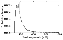
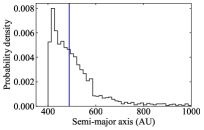
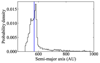
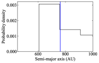
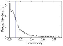
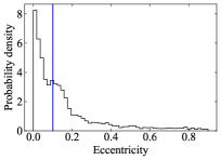
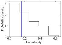
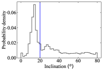
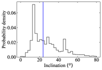
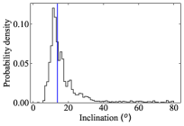
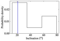
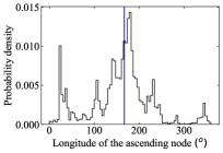
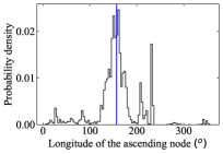
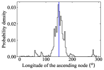
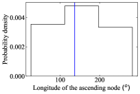
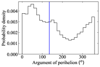
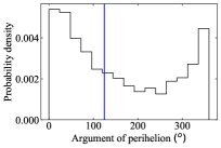
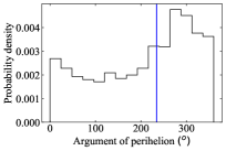
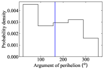
Figure 1: Barycentric orbital elements of putative perturber planets. Distributions of barycentric orbital elements of planetary orbits that may result in close encounters (under 5 AU for $q_{\rm p}>300$ AU, under 7.5 AU for $q_{\rm p}>400$ AU, and under 10 AU for $q_{\rm p}>500$ AU and $q_{\rm p}>600$ AU) with five or more present-day extreme trans-Neptunian objects (ETNOs). Each column of panels shows the cumulative results of 2$\times$10¹⁰ experiments. From left to right, the panels show the results of imposing $q_{\rm p}>300$ AU (left column, 20304 orbits), $q_{\rm p}>400$ AU (5671 orbits), $q_{\rm p}>500$ AU (2635 orbits), and $q_{\rm p}>600$ AU (right column, 56 orbits). Median values are shown as vertical blue lines. Based on the available data on known ETNOs, the presence of massive perturbers well beyond 600 AU is strongly excluded within the context of the hypotheses centered in this study.

Table 1: Summary of central values and dispersions of optimal barycentric orbits.

Orbital parameter	$q_{\rm p}>300$ AU	$q_{\rm p}>400$ AU	$q_{\rm p}>500$ AU	$q_{\rm p}>600$ AU
Semi-major axis, $a_{\rm p}$ (AU)	375${}_{-44}^{+111}$ (376)	489${}_{-64}^{+130}$ (420)	569${}_{-31}^{+55}$ (581)	762${}_{-120}^{+279}$ (680)
Eccentricity, $e_{\rm p}$	0.10${}_{-0.07}^{+0.21}$ (0.01)	0.10${}_{-0.08}^{+0.19}$ (0.01)	0.05${}_{-0.03}^{+0.09}$ (0.02)	0.16${}_{-0.13}^{+0.19}$ (0.07)
Inclination, $i_{\rm p}$ (°)	20${}_{-8}^{+34}$ (14)	24${}_{-10}^{+22}$ (14)	14${}_{-3}^{+9}$ (12)	21${}_{-6}^{+52}$ (24)
Longitude of the ascending node, $\Omega_{\rm p}$ (°)	167${}_{-70}^{+44}$ (180)	157${}_{-23}^{+48}$ (161)	149${}_{-17}^{+18}$ (148)	137${}_{-55}^{+141}$ (156)
Argument of perihelion, $\omega_{\rm p}$ (°)	135${}_{-94}^{+170}$ (51)	124${}_{-94}^{+193}$ (12)	234${}_{-165}^{+81}$ (275)	164${}_{-106}^{+109}$ (56)

Table 1 shows a summary of the central values and dispersions of the orbital parameters of the sample of orbits that may experience close encounters with multiple known ETNOs. We consider that results for $q_{\rm p}>300$ AU and $q_{\rm p}>400$ AU are statistically consistent and are compatible with $a_{\rm p}\in(331,489)$ AU, $e_{\rm p}<0.1$, $i_{\rm p}\in(10\degr,20\degr)$, $\Omega_{\rm p}$$\sim$180°, and $\omega_{\rm p}\in(-60{\degr},60{\degr})$. The value of $a_{\rm p}$ is probably $\sim$400 AU but the uncertainty is significant, the value of the eccentricity is well constrained and it has to be low, the inclination is perhaps the best constrained value and it is $\sim$14°, the value of $\Omega_{\rm p}$ is very likely $\sim$180°, but the value of $\omega_{\rm p}$ is poorly constrained, perhaps $\sim$50°. If scattering is the main source of orbital modification for the group of ETNOs that mainly move at (300, 400) AU from the Sun, the orbit of the putative perturber is relatively well-constrained and according to Fienga et al. (2020), it must have a mass $<5\leavevmode\nobreak\ M_{\oplus}$.

Table 1 shows that our approach is far less conclusive in the cases of $q_{\rm p}>500$ AU and $q_{\rm p}>600$ AU as these values produce distributions of the orbital parameters that may not be statistically compatible. In any case, we must emphasize that $>50$% of the known ETNOs cannot interact directly with a perturber with $q_{\rm p}>500$ AU because their aphelion distances, $Q=a\,(1+e)$, are below 500 AU: 9 ETNOs have $Q<300$ AU, 18 have $Q<400$ AU, and 23 have $Q<500$ AU. Therefore, the distribution in $Q$ and our calculations suggest that more than one perturber is required if scattering is the main source of orbital modification for the known ETNOs. Perturbers might not be located farther than 600 AU and they have to follow moderately eccentric and inclined orbits to be capable of experiencing present-day close encounters with multiple known ETNOs.

At this point, it can be argued that the results in Fig. 1 may be affected by a statistical artifact. In order to test the statistical significance of our results, we repeated the Monte Carlo random search on an input sample of scrambled data as explained in Appendix D. By randomly reassigning the values of the orbital elements of the ETNOs, we preserve the original distributions of the parameters, but destroy any possible correlations that may have been induced by close encounters with massive perturbers (or the effects of hypothetical mean-motion or secular resonances). The results of this significance test are shown in Fig. 3: the distribution of $i_{\rm p}$ becomes flat and almost the same happens to the distribution of $\Omega_{\rm p}$. In other words, for the scrambled data, it is not possible to find a statistically significant orbital solution that is compatible with the starting hypothesis and we conclude that the results in Fig. 1 are unlikely to be due to statistical artifacts.

4 Summary and conclusions

When considering the well-studied case of Neptune and the regular trans-Neptunian objects, we observe that these objects are not part of a single population, but they are organized into several dynamical classes. Some objects never experience close encounters with Neptune due to the existence of protection mechanisms such as mean-motion or secular resonances, as in the case of Neptune’s Trojans or Pluto (see e.g., Milani et al. 1989; Wan et al. 2001), others undergo close encounters that may send them towards the inner solar system (centaurs) or outwards to become scattered objects (see the recent review by Saillenfest 2020). If trans-Plutonian planets exist, their perturbations may shape the extreme trans-Neptunian space in a similar fashion and the current sample of ETNOs may include the signatures of their presence (see e.g. Saillenfest et al. 2017).

Our results show that it is possible to find suitable orbits for which the mutual nodal distances of sizeable ($\geq 5$, comprising at least 13% of the sample) groups of ETNOs with their assumed perturber could be small enough for a close encounter to occur, at least in theory (assuming that no protection mechanisms, such as mean-motion or secular resonances, are in place to avoid the flyby). This was our original aim. In addition, the results presented in Sect. 3 clearly indicate that the most probable planetary orbit consistent with the starting hypothesis is the one obtained for the experiment with $q_{\rm p}>300$ AU. The number of consistent orbits in this case is 3.6 times higher than the one found for $q_{\rm p}>400$ AU. Our results seem to be incompatible with those attributed to a statistical artifact (see Appendix D).

Prior to the announcement of the Planet 9 hypothesis (Batygin & Brown 2016), Trujillo & Sheppard (2014) had already argued for the existence of a planet at 250 AU within the context of the ETNOs — driving von Zeipel-Lidov-Kozai librations on 2012 VP₁₁₃ — and de la Fuente Marcos & de la Fuente Marcos (2014) suggested that the limited data available at the time were more compatible with the presence of two massive perturbers, one of them close to 300 AU. These massive perturbers were initially proposed based on data corresponding to a sample of 13 objects, whereas the current sample has tripled this number. If we repeat the experiment discussed in Sect. 3 for $q_{\rm p}>200$ AU (see Appendix E), we find that the number of consistent orbits, although larger than the one generated in the experiment for $q_{\rm p}>400$ AU, is still lower than that of the most statistically significant case, namely, 8234 versus 20304 for $q_{\rm p}>300$ AU. The most likely orbit is still similar, in terms of shape and orientation in space, to the most probable one in the $q_{\rm p}>300$ AU case.

Our results are consistent with the conclusions of the study presented in de la Fuente Marcos & de la Fuente Marcos (2017). Although our approach has not been able to single out a statistically significant, unique planetary orbit that may be responsible for the orbital architecture observed in extreme trans-Neptunian space, we provide narrow ranges for the orbital parameters of putative planets that may have experienced orbit-changing encounters with known ETNOs. Some sections of the available orbital parameter space are strongly excluded by the findings of our analysis.

Appendix A Mutual nodal distance: formulae

Our statistical analyses are based on studying the distribution of nodal distances between two Keplerian trajectories (one ETNO and one hypothetical planet) with a common focus; therefore, the core of our approach is purely geometrical and gravitational interactions are not directly taken into account. The mutual nodal distance between the orbits of a small body (an ETNO in our case) and an arbitrary planet can be written as (see Eqs. 16 and 17 in Saillenfest et al. 2017):

$${\Delta}d_{\rm pn}=\frac{a\ (1-e^{2})}{1\pm e\ \cos{\varpi}}-\frac{a_{\rm p}\ (1-e_{\rm p}^{2})}{1\pm e_{\rm p}\ \cos{\varpi_{\rm p}}}\,,$$ (1)

where

$\Delta\Omega_{\rm p}=\Omega-\Omega_{\rm p}$, and $a$, $e$, $i$, $\Omega$ and $\omega$ are the orbital elements of the small body, and $a_{\rm p}$, $e_{\rm p}$, $i_{\rm p}$, $\Omega_{\rm p}$, and $\omega_{\rm p}$ those of the arbitrary planet. For each random search experiment (each analysis consists of 2$\times$10¹⁰), we compute the orbital elements of the putative perturber using the expressions:

$$q_{\rm p} =x+(1000-x)\,r_{1}$$ (4)

$$e_{\rm p} =0.9\,r_{2}$$

$$a_{\rm p} =q_{\rm p}/(1-e_{\rm p})$$

$$i_{\rm p} =80\,r_{3}$$

$$\Omega_{\rm p} =360\,r_{4}$$

$$\omega_{\rm p} =360\,r_{5}\,,$$

where $x=300,400,500,$ and 600 AU (see Sect. 2, or 200 AU for Appendix E), and $r_{j}$ with $j=1,5$, are random numbers in the interval (0, 1) with a uniform distribution.

Appendix B Extreme trans-Neptunian objects: Data

The barycentric orbit determinations used as input data in the uniform Monte Carlo random search discussed in Sect. 3 are shown in Table 2. The data are referred to epoch 2459000.5 Barycentric Dynamical Time (TDB) and they have been retrieved (as of 11-January-2021) from JPL’s SBDB and HORIZONS using tools provided by the Python package Astroquery (Ginsburg et al. 2019).

Table 2: Barycentric orbital elements and 1$\sigma$ uncertainties of known ETNOs with robust orbit determinations.

Object	$a_{\rm b}$	$\sigma_{a}$	$e_{\rm b}$	$\sigma_{e}$	$i_{\rm b}$	$\sigma_{i}$	$\Omega_{\rm b}$	$\sigma_{\Omega}$	$\omega_{\rm b}$	$\sigma_{\omega}$
	(AU)	(AU)			(°)	(°)	(°)	(°)	(°)	(°)
82158 (2001 FP185)	215.548928	0.040005	0.841097	2.7618$\times$10-5	30.800299	3.259$\times$10-5	179.358499	4.3407$\times$10-5	6.874579	0.00045074
90377 Sedna	506.424770	0.18758	0.849551	6.2014$\times$10-5	11.928524	3.7219$\times$10-6	144.401511	0.00055761	311.285511	0.0035418
148209 (2000 CR105)	221.976439	0.6072	0.801226	0.00056946	22.755910	0.00058664	128.285827	0.00029583	316.690118	0.011843
445473 (2010 VZ98)	153.432684	0.011897	0.776116	1.7043$\times$10-5	4.510568	9.5639$\times$10-6	117.394668	0.00038454	313.728058	0.00069884
474640 (2004 VN112)	327.713834	1.5617	0.855596	0.00067208	25.547962	0.00027987	66.022244	0.00043186	326.987949	0.00928245
496315 (2013 GP136)	150.177337	0.18997	0.726731	0.00037413	33.538905	0.00064333	210.727262	0.00010633	42.569086	0.03727751
505478 (2013 UT15)	200.156721	0.80063	0.780530	0.0010167	10.652044	0.0010304	191.954169	0.00038493	252.123877	0.032992
506479 (2003 HB57)	159.594669	0.36652	0.761283	0.00050502	15.500384	0.00027768	197.871006	0.00037845	10.837414	0.008816
508338 (2015 SO20)	164.785707	0.020652	0.798712	2.404$\times$10-5	23.410688	3.432$\times$10-5	33.634139	1.895$\times$10-5	354.827026	0.00055221
523622 (2007 TG422)	502.465990	0.2381	0.929226	3.4842$\times$10-5	18.595364	3.1757$\times$10-5	112.910531	0.00012321	285.664088	0.00090846
527603 (2007 VJ305)	192.002016	0.047887	0.816750	4.288$\times$10-5	11.983654	6.5092$\times$10-5	24.382506	3.1038$\times$10-5	338.356121	0.00089984
541132 Leleakuhonua	1077.120640	111.53	0.939677	0.0063597	11.671280	0.00063416	300.993671	0.0071997	117.944434	0.3158
2002 GB32	206.586429	0.51121	0.828932	0.00038669	14.192110	0.00015226	177.043472	0.00033413	37.047917	0.0046496
2003 SS422	203.255204	148.31	0.806561	0.16161	16.781709	0.14714	151.041519	0.17403	211.597889	43.173
2005 RH52	153.565757	0.21296	0.746072	0.00032216	20.445652	0.00036748	306.109904	0.00088931	32.512598	0.00767
2010 GB174	351.380200	22.505	0.861811	0.010215	21.562661	0.0051779	130.715273	0.019788	347.236662	0.36426
2012 VP113	262.065255	1.4232	0.692739	0.0019759	24.052063	0.0023167	90.802707	0.0056	293.924997	0.37222
2013 FS28	191.761394	98.598	0.821344	0.0969	13.068232	0.02486	204.638126	0.016117	102.176514	2.4905
2013 FT28	294.523622	10.063	0.852396	0.005059	17.375255	0.0034261	217.722701	0.0048316	40.696900	0.16454
2013 RF98	363.869961	13.352	0.900799	0.0036143	29.538492	0.0033747	67.635472	0.0053263	311.757065	0.66841
2013 RA109	462.902530	2.2525	0.900602	0.00046151	12.399719	0.00011973	104.798695	0.005524	262.917813	0.15134
2013 SY99	729.233540	24.996	0.931474	0.0024376	4.225431	0.0011969	29.509257	0.0052081	32.141187	0.11464
2013 SL102	314.359140	0.70133	0.878709	0.00025008	6.504915	7.5898$\times$10-5	94.730847	0.0056732	265.496106	0.055127
2013 UH15	173.746767	8.3586	0.798455	0.011307	26.080589	0.0057534	176.542268	0.0071993	282.865545	0.27819
2014 FE72	1548.667877	440.14	0.976632	0.0087352	20.632449	0.0028763	336.829059	0.0051919	133.959137	0.064528
2014 SR349	298.050876	19.924	0.840461	0.010668	17.967979	0.0017476	34.886583	0.014948	341.238334	0.6312
2014 WB556	279.905880	2.5421	0.847464	0.0013182	24.157500	0.00019211	114.891154	0.0033985	235.333796	0.056364
2015 BP519	448.721566	8.3963	0.921446	0.0016417	54.110682	9.9809$\times$10-5	135.213150	0.0018968	348.058562	0.027567
2015 GT50	311.140075	2.6471	0.876545	0.0010976	8.794999	0.0012014	46.064057	0.0028595	128.986870	0.11107
2015 KG163	680.351485	5.8808	0.940483	0.00037323	13.994347	0.0011581	219.103229	0.0017119	32.110680	0.098552
2015 KH163	152.922061	0.59238	0.738806	0.0011085	27.137445	0.0013782	67.572913	0.00060792	230.813811	0.048894
2015 RX245	423.304136	4.7739	0.892386	0.0013068	12.138092	0.0019317	8.605207	0.0001895	65.120605	0.045144
2015 RY245	225.301756	4.5912	0.861023	0.0028285	6.030530	0.0010408	341.532143	0.005986	354.533793	0.24642
2016 GA277	154.842684	6.8842	0.767982	0.011305	19.421077	0.00034091	112.841139	0.019248	178.521618	0.11573
2016 QU89	171.465345	0.33356	0.794425	0.00040081	16.975710	0.00046385	102.898107	0.0035642	303.349937	0.082868
2016 QV89	171.616289	0.22913	0.767183	0.00036545	21.387605	0.00041616	173.215227	0.0011962	281.086675	0.019706
2016 SG58	232.948888	0.40228	0.849292	0.00027193	13.220892	4.9315$\times$10-5	118.978173	0.0023883	296.291522	0.035779
2016 TP120	174.578585	24.948	0.771693	0.038036	32.639476	0.0005895	126.728289	0.027144	350.990565	0.39834
2018 VM35	261.464338	64.008	0.827901	0.050434	8.479536	0.0033767	192.409778	0.058367	302.700112	2.6758

The orbits of the synthetic ETNOs are obtained using the expressions:

$$a_{\rm s} =a_{\rm b}+\sigma_{a}\,R_{1}$$ (5)

$$e_{\rm s} =e_{\rm b}+\sigma_{e}\,R_{2}$$

$$i_{\rm s} =i_{\rm b}+\sigma_{i}\,R_{3}$$

$$\Omega_{\rm s} =\Omega_{\rm b}+\sigma_{\Omega}\,R_{4}$$

$$\omega_{\rm s} =\omega_{\rm b}+\sigma_{\omega}\,R_{5}\,,$$

where $R_{j}$ with $j=1,5$, are univariate Gaussian random numbers.

Appendix C Heliocentric orbit determinations: results

If we repeat the calculations discussed in Sect. 3 using heliocentric orbit determinations instead of barycentric ones as input data, we obtain the distributions in Fig. 2 with central values and dispersions summarized in Table 3.

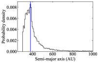
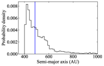
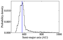
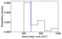
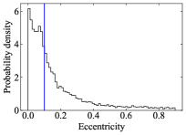
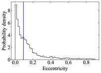
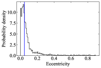
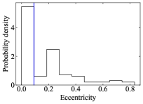
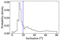
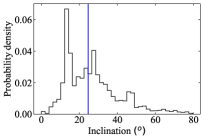
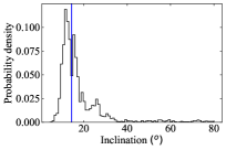
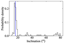
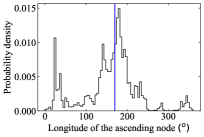
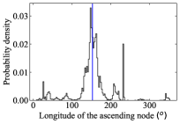
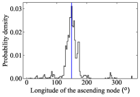
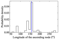
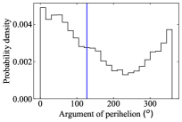
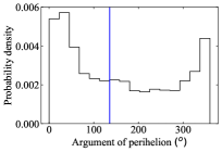
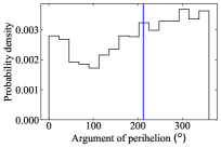
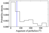
Figure 2: Heliocentric orbital elements of putative perturber planets. Distributions of heliocentric orbital elements of planetary orbits that may result in close encounters (under 5 AU for $q_{\rm p}>300$ AU, under 7.5 AU for $q_{\rm p}>400$ AU, and under 10 AU for $q_{\rm p}>500$ AU and $q_{\rm p}>600$ AU) with five or more present-day extreme trans-Neptunian objects (ETNOs). Each column of panels shows the cumulative results of 2$\times$10¹⁰ experiments. From left to right, the panels show the results of imposing $q_{\rm p}>300$ AU (left column, 18369 orbits), $q_{\rm p}>400$ AU (6594 orbits), $q_{\rm p}>500$ AU (3567 orbits), and $q_{\rm p}>600$ AU (right column, 105 orbits). Median values are shown as vertical blue lines. Based on the available data on known ETNOs, the presence of massive perturbers well beyond 600 AU is strongly excluded within the context of the hypotheses centered in this study.

Table 3: Summary of central values and dispersions of optimal heliocentric orbits.

Orbital parameter	$q_{\rm p}>300$ AU	$q_{\rm p}>400$ AU	$q_{\rm p}>500$ AU	$q_{\rm p}>600$ AU
Semi-major axis, $a_{\rm p}$ (AU)	379${}_{-47}^{+112}$ (378)	486${}_{-62}^{+129}$ (420)	576${}_{-29}^{+45}$ (584)	684${}_{-65}^{+299}$ (645)
Eccentricity, $e_{\rm p}$	0.10${}_{-0.07}^{+0.21}$ (0.01)	0.09${}_{-0.07}^{+0.18}$ (0.01)	0.05${}_{-0.03}^{+0.08}$ (0.04)	0.09${}_{-0.08}^{+0.25}$ (0.05)
Inclination, $i_{\rm p}$ (°)	19${}_{-7}^{+32}$ (13)	25${}_{-11}^{+17}$ (13)	14${}_{-3}^{+10}$ (12)	17${}_{-1}^{+17}$ (16)
Longitude of the ascending node, $\Omega_{\rm p}$ (°)	170${}_{-77}^{+37}$ (181)	153${}_{-19}^{+24}$ (148)	150${}_{-16}^{+19}$ (151)	157${}_{-26}^{+5}$ (160)
Argument of perihelion, $\omega_{\rm p}$ (°)	127${}_{-92}^{+180}$ (7)	136${}_{-107}^{+179}$ (35)	212${}_{-148}^{+102}$ (305)	62${}_{-33}^{+144}$ (22)

Appendix D Statistical significance

In order to verify that our results do not come from statistical artifacts, we randomly scramble the orbit parameters data used as input and repeat the uniform Monte Carlo random searches discussed in Sect. 3 and Appendix C. In these experiments, the set of synthetic ETNOs is such that, for example, the first object may have the value of $a$ of object #5, $e$ of #27, $i$ of #7, $\Omega$ of #37, and $\omega$ of #13. By randomly rearranging the values of the orbital elements of the ETNOs, we retain the original distributions of the parameters, but destroy any possible correlations existing among them. The results of these statistical significance tests are shown in Figs. 3 and 4. The distributions in $i_{\rm p}$ and $\Omega_{\rm p}$ are flattened and no statistically significant perturbing orbits are produced.

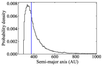
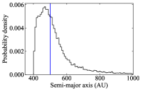
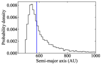
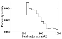
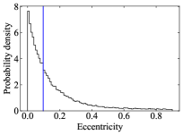
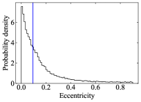
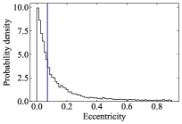
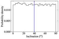
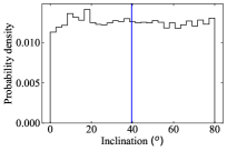
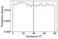
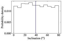
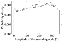
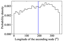
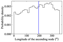
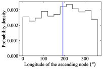
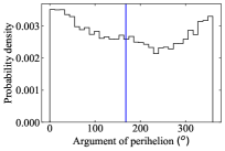
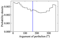
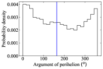
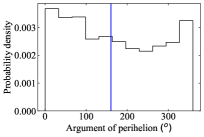
Figure 3: Barycentric orbital elements of putative perturber planets. As Fig. 1 but using scrambled data as input.

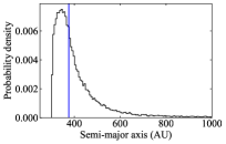
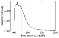
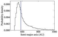
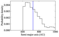
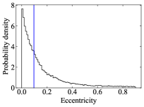
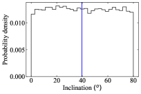
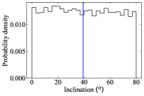
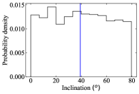
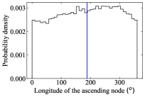
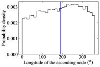
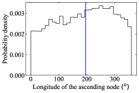
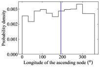
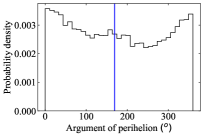
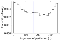
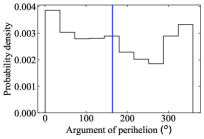
Figure 4: Heliocentric orbital elements of putative perturber planets. As Fig. 2 but using scrambled data as input.

Appendix E Results at 200 AU

Fienga et al. (2020) focused on testing for the presence of possible planets at 400, 500, 600, 650, 700, 750, and 800 AU with masses of 5 or 10 $M_{\oplus}$. The existence of 5 $M_{\oplus}$ planets at 400 or 500 AU is strongly disfavored by their results (see their Fig. 5, top panels). However, a hypothetical Earth-like planet at 200–400 AU from the Sun may still induce significant gravitational effects if close encounters are possible, due to its relatively large value for the Hill radius (e.g., 2.2 AU if $a_{\rm p}=200$ AU, $e_{\rm p}=0.1$ and 1 $M_{\oplus}$). We repeated the analysis, imposing $q_{\rm p}>200$ AU, and we obtained 8234 orbits with a number of potential close approaches in the range between 5–7. Here, we count how many synthetic ETNOs had at least one mutual nodal distance with the planet under 2 AU. The median values and 16th and 84th percentiles (absolute maximum in parentheses) from the Monte Carlo random searches whose distributions are shown in Fig. 5 are: $a_{\rm p}=272_{-38}^{+94}$ AU (258 AU), $e_{\rm p}=0.12_{-0.08}^{+0.21}$ (0.03), $i_{\rm p}=28{\degr}_{-18\degr}^{+35\degr}$ (10°), $\Omega_{\rm p}=194{\degr}_{-90\degr}^{+58\degr}$ (196°), and $\omega_{\rm p}=179{\degr}_{-130\degr}^{+132\degr}$ (350°).

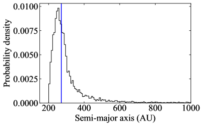
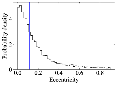
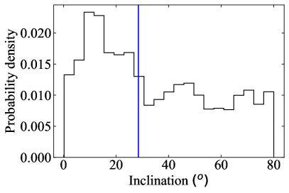
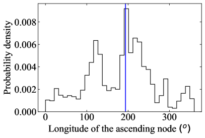
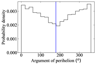
Figure 5: Barycentric orbital elements of putative perturber planets. As Fig. 1 but for $q_{\rm p}>200$ AU.