Introduction to Neural Transfer Learning with Transformers for Social Science Text Analysis

Abstract. Transformer-based models for transfer learning have the potential to achieve high prediction accuracies on text-based supervised learning tasks with relatively few training data instances. These models are thus likely to benefit social scientists that seek to have as accurate as possible text-based measures but only have limited resources for annotating training data. To enable social scientists to leverage these potential benefits for their research, this paper explains how these methods work, why they might be advantageous, and what their limitations are. Additionally, three Transformer-based models for transfer learning, BERT (Devlin et al., 2019), RoBERTa (Liu et al., 2019), and the Longformer (Beltagy et al., 2020), are compared to conventional machine learning algorithms on three applications. Across all evaluated tasks, textual styles, and training data set sizes, the conventional models are consistently outperformed by transfer learning with Transformers, thereby demonstrating the benefits these models can bring to text-based social science research.

Keywords. Natural language processing, deep learning, neural networks, transfer learning, Transformer, BERT

Source Code. The code of this study is openly available at https://doi.org/10.6084/m9.figshare.14394173

Acknowledgements. I am very grateful to Paul W. Thurner, Christian Heumann, Matthias Aßenmacher, the participants of the colloquium at the chair of Paul W. Thurner, and three anonymous reviewers for their highly valuable guidance and helpful comments on this work.

Funding. This work was supported by a scholarship I received from the German Academic Scholarship Foundation.

1 Introduction: Why Neural Transfer Learning with Transformers?

In social science, supervised learning techniques have been employed to measure a vast range of application-specific (and often complex, latent, and multidimensional) concepts from texts, such as e.g. tonality (Rudkowsky et al., 2018; Barberá et al., 2021; Fowler et al., 2021), inequality (Nelson et al., 2021), populism (Di Cocco & Monechi, 2021), attitudes (Ceron et al., 2014; Mitts, 2019), policy topics (Osnabrügge et al., 2021; Sebők & Kacsuk, 2021), and events (D’Orazio et al., 2014; Zhang & Pan, 2019; Muchlinski et al., 2021). In such supervised learning settings, the training data encode how the concept (e.g. attitude, inequality, event) is to be operationalized and the text analysis method is the measurement method that is deployed to assign the textual units to the values of the variable.

If a researcher is applying a supervised learning method on text data for the purpose of measuring an a priori-specified concept, her aim—as in any measurement process—will be to have a valid measure that captures the concept it is devised to measure. And consequently—because when working with text data humans are usually seen as the “the ultimate arbiter of the ‘validity’ of any research exercise” (Benoit, 2020, p. 470)—the aim for the researcher is to have a supervised learning technique that as closely as possible can imitate human codings (Grimmer & Stewart, 2013, p. 270, 279). After having trained a model on human annotated training data, the researcher thus will hope that the trained model as accurately as possible predicts human codings on data that have not been used in training (Grimmer & Stewart, 2013, p. 271, 279). If this is the case and hence the model can be said to generalize well, this indicates that the model’s predictions will provide a valid measure of the concept under study (Grimmer & Stewart, 2013, p. 271, 279).

In the field of natural language processing (NLP), the usage of deep learning models (as compared to conventional machine learning algorithms) has enabled researchers to learn better generalizing mappings from textual inputs to task-specific outputs and hence has enabled researchers to more accurately perform a wide spectrum of prediction tasks such as text classification, machine translation, or reading comprehension (Goldberg, 2016, p. 347-348; Ruder, 2020). Despite the fact that deep learning techniques tend to exhibit higher prediction accuracies in text-based supervised learning tasks compared to traditional machine learning algorithms (Socher et al., 2013; Iyyer et al., 2014; Budhwar et al., 2018; Ruder, 2020), they are not yet a standard tool for social science researchers that use supervised learning for text analysis. Although there are exceptions (e.g. Rudkowsky et al., 2018; Zhang & Pan, 2019; Amsalem et al., 2020; Chang & Masterson, 2020; Muchlinski et al., 2021; Wu & Mebane, 2021), social scientists typically resort to bag-of-words-based representations of texts that serve as an input to conventional machine learning models such as support vector machines (SVMs), naive Bayes, random forests, boosting algorithms, or regression with regularization (see e.g. Diermeier et al., 2011; Colleoni et al., 2014; D’Orazio et al., 2014; Ceron et al., 2015; Theocharis et al., 2016; Welbers et al., 2017; Kwon et al., 2018; Greene et al., 2019; Katagiri & Min, 2019; Mitts, 2019; Pilny et al., 2019; Ramey et al., 2019; Rona-Tas et al., 2019; Anastasopoulos & Bertelli, 2020; Miller et al., 2020; Park et al., 2020; Barberá et al., 2021; Di Cocco & Monechi, 2021; Fowler et al., 2021; Osnabrügge et al., 2021; Sebők & Kacsuk, 2021).

One among several likely reasons why deep learning methods so far have not been widely used for text-based supervised learning tasks by social scientists might be that deep learning models have considerably more parameters to be learned in training than classic machine learning models. Consequently, deep learning models are computationally highly intensive and require substantially larger numbers of training examples. Goodfellow et al., (2016, p. 20) stated that “As of 2016, a rough rule of thumb is that a supervised deep learning algorithm will generally achieve acceptable performance with around 5,000 labeled examples per category”. For research questions relating to domains in which it is difficult to access or label large enough numbers of training data instances, deep learning becomes infeasible or prohibitively costly.

Recent developments within NLP on transfer learning alleviate this problem. Transfer learning is a set of learning procedures in which knowledge that has been learned from training on a source task in a source domain is used to improve learning on the target task in the target domain (where the target task is the task of interest that a researcher

actually seeks to conduct) (Pan & Yang, 2010, p. 1347). In sequential transfer learning—which is one common type of transfer learning—the aim when training on a source task is to acquire a highly general, close to universal language representation model (Ruder, 2019a , p. 64). The pretrained general-purpose representation model then can be used as an input to a target task of interest (Ruder, 2019a , p. 63-64). This practice of using a pretrained language model as an initialization for training on a target task has been shown to improve the prediction performances on a large variety of NLP target tasks (Ruder, 2020; Bommasani et al., 2021, p. 22-23). Moreover, adapting a pretrained language model to a target task requires fewer target training examples than when not using transfer learning and training the model from scratch on the target task (Howard & Ruder, 2018, p. 334).

In addition to the efficiency and performance gains from research on transfer learning, the introduction of the attention mechanism (Bahdanau et al., 2015) and the self-attention mechanism (Vaswani et al., 2017) has significantly improved the ability of deep learning NLP models to capture contextual information from texts. (Self-)attention mechanisms learn a token representation by capturing information from other tokens, and thereby encode textual dependencies and context-dependent meanings. (Self-)attention mechanisms constitute the core building blocks of the Transformer—a type of deep learning model that has been presented by Vaswani et al., in 2017. During the last years, several Transformer-based models that are used in a transfer learning setting have been introduced (e.g. Devlin et al., 2019; Liu et al., 2019; Yang et al., 2019). These models substantively outperform previous state-of-the-art models across a large variety of NLP tasks (Ruder, 2020; Bommasani et al., 2021, p. 22-23).

Due to the likely increases in prediction accuracy, as well as the efficient and less resourceful adaptation phase, transfer learning with deep (e.g. Transformer-based) language representation models seems promising to social science researchers. It seems especially promising to researchers that seek to have as accurate as possible text-based measures but lack the resources to annotate large amounts of data or are interested in specific domains in which only small corpora and few training instances exist. In order to equip social scientists to use the potential of transfer learning with Transformer-based models for their research, this paper provides an introduction to transfer learning and the Transformer.

The following Section 2 compares conventional machine learning to deep learning by focusing on the question of how textual features (e.g. characters, terms, symbols) and larger textual units (e.g. sentences, paragraphs, tweets, comments, speeches, … here named: documents) tend to be represented in conventional vs. deep learning approaches. The subsequent Section 3 on transfer learning provides an answer to the question of what transfer learning is and explains in more detail in what ways transfer learning might be beneficial. The then following Section 4 introduces the attention mechanism and the Transformer and elaborates on how the Transformer has advanced the study of text. Afterward, an overview of Transformer-based models for transfer learning is provided (Section 5). Here, a special focus will be given to the seminal Transformer-based language representation model BERT (standing for Bidirectional Encoder Representations from Transformers) (Devlin et al., 2019). Additionally, the changes in NLP and artificial intelligence (AI) research, that these models have caused, are outlined and problematic aspects are discussed. Finally, three Transformer-based models for transfer learning, BERT (Devlin et al., 2019), RoBERTa (Liu et al., 2019), and the Longformer (Beltagy et al., 2020), are compared to traditional learning algorithms based on three classification tasks using data from speeches in the UK parliament (Duthie & Budzynska, 2018), tweets regarding the legalization of abortion (Mohammad et al., 2017), and comments from Wikipedia Talk pages (Jigsaw/Conversation AI, 2018) (Section 6). The final Section 7 concludes with a discussion on task-specific factors and research goals for which neural transfer learning with Transformers is highly beneficial vs. rather limited. Throughout the paper, it is assumed that readers know core elements of neural network architectures, and are also familiar with recurrent neural networks (RNNs) as well as with optimization via stochastic gradient descent with backpropagation. For readers that feel not sufficiently acquainted with these deep learning concepts see Appendix A. Also note that a document is an ordered sequence of tokens and here is denoted as $d_{i}=(a_{1},\dots,a_{t},\dots,a_{T})$. A token $a_{t}$ is an instance of a type, which is the set of all tokens that are made up of the same string of characters (Manning et al., 2008, p. 22). A type that is used for analysis is named term or feature and here is given as $z_{u}$. The set of features that are used in an analysis is $\{z_{1},\dots,z_{u}\dots,z_{U}\}$.

2 Conventional Machine Learning vs. Deep Learning

2.1 Conventional Machine Learning

Given raw input data $D=(d_{1},\dots,d_{i},\dots,d_{N})$ (e.g. a corpus comprising $N$ raw text files) and a corresponding output variable $\bm{y}=[y_{1},\dots,y_{i},\dots,y_{N}]^{\top}$ (e.g. class labels), the aim in supervised machine learning is to find the parameters $\bm{\theta}$ of a function $f$ that captures the general systematic relation between $D$ and $\bm{y}$ such that the trained model will generalize well and generate accurate predictions for new, yet unseen data $D_{test}$ (James et al., 2013, p. 30; Chollet, 2021, ch. 1.1.3).

When applying a machine learning algorithm in order to learn a function that as accurately as possible maps from text data inputs to provided outputs, the algorithm, however, will not take as an input raw text documents. The raw text units first have to be converted into a format that is suitable for data analysis (Benoit, 2020, p. 463-464). This is achieved by transforming each raw data unit $d_{i}$ into an abstracted representation of $d_{i}$ (Benoit, 2020, p. 463-464). Learning in supervised machine learning hence essentially is a two-step process (Goodfellow et al., 2016, p. 10): The first step is to create or learn representations of the data, and the second step is to learn mappings from these representations of the data to the output. For a single document $d_{i}$, the first step can be described as $\mathsf{f}_{l}(d_{i},\bm{\hat{\theta}}_{l})$ and the entire process as

$$\hat{y}_{i}=\mathsf{f}(d_{i},\bm{\hat{\theta}})=\mathsf{f}_{o}(\mathsf{f}_{l}(d_{i},\bm{\hat{\theta}}_{l}),\bm{\hat{\theta}}_{o})$$ (1)

where the subscript $l$ indicates the mapping from raw data to a representation and the subscript $o$ indicates the mapping from the representation to the output. Conventional machine learning algorithms cover the second step: They learn a function mapping data representations to the output. This in turn implies that the first step falls to the researcher who has to (manually) generate representations of the data herself.

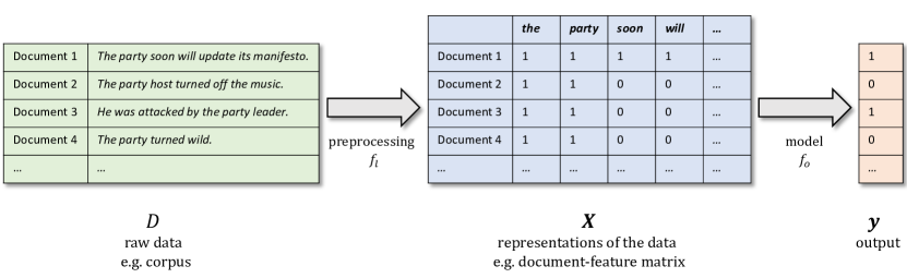
Figure 1: Learning as a Two-Step Process. In text-based applications of conventional machine learning approaches, the raw data $D$ first are (manually) preprocessed such that each example is represented as a feature vector in the document-feature matrix $\bm{X}$. Second, these representations of the data are fed as inputs to a traditional machine learning algorithm that learns a mapping between data representations $\bm{X}$ and outputs $\bm{y}$.

When working with texts, the raw data $D$ are typically a corpus of text documents. A very common approach in social science is to transform the raw text files via multiple preprocessing procedures into a document-feature matrix $\bm{X}=[\bm{x}_{1}|\dots|\bm{x}_{i}|\dots|\bm{x}_{N}]^{\top}$ (see Figure 1) (Benoit, 2020, p. 464). In a document-feature matrix, each document is represented as a feature vector $\bm{x}_{i}=[x_{i1},\dots,x_{iu},\dots,x_{iU}]$ (Turney & Pantel, 2010, p. 147). Element $x_{iu}$ in this vector gives the value of the $i$th document on the $u$th textual feature—and typically is the (weighted) number of times that the $u$th feature occurs in the $i$th document (Turney & Pantel, 2010, p. 143, 147). To conduct the second learning step, the researcher then commonly applies a conventional machine learning algorithm on the document-feature matrix to learn the relation between the document-feature representation of the data $\bm{X}$ and the provided response values $\bm{y}$.

There are three difficulties with this approach. The first is that it may be hard for the researcher to a priori know which features are useful for the task at hand (Goodfellow et al., 2016, p. 3-5). The performance of a supervised learning algorithm will depend on the representation of the data in the document-feature matrix (Goodfellow et al., 2016, p. 3-4). In a classification task, features that capture observed linguistic variation that helps in assigning the texts into the correct categories are more informative and will lead to a better classification performance than features that capture variation that is not helpful in distinguishing between the classes (Goodfellow et al., 2016, p. 3-5). Yet determining which sets of possibly highly abstract and complex features are informative (and which are not) is highly difficult (Goodfellow et al., 2016, p. 3-5). A researcher can choose from a multitude of possible preprocessing steps such as stemming, lowercasing, removing stopwords, adding POS tags, or applying a sentiment lexicon. Social scientists may be able to use some of their domain knowledge in deciding upon a few specific preprocessing decisions (e.g. whether it is likely that excluding a predefined list of stopwords will be beneficial because it reduces dimensionality or will harm performance because the stopword list includes terms that are important). Domain knowledge, however, is most unlikely to guide researchers regarding all possible permutations of preprocessing steps. Simply trying out each possible preprocessing permutation in order to select the best performing one for a supervised task is not possible given the massive number of permutations and limited researcher resources.

Second, the document-feature matrix defines a representational space in which each feature constitutes one separate and independent dimension of the space (Goldberg, 2016, p. 349-350). Accordingly, if there are $U$ features, $\{z_{1},\dots,z_{u},\dots,z_{U}\}$, then each feature $z_{u}$ defines one dimension of the representational space. This implies that each feature is represented to be as distant (and thus as dissimilar) to one feature as to each other feature (Goldberg, 2016, p. 351). The terms ‘excellent’ and ‘outstanding’ are treated as (dis)similar to each other as the terms ‘excellent’ and ‘terrible’. Moreover, as—even after feature exclusion and feature normalization—the number of features in any text-based analysis typically tends to be high, the document representation vectors $\bm{x}_{i}$ tend to be high-dimensional and sparse. (This is, $\bm{x}_{i}$ is likely to be a vector with a large number of elements, most of which will be zero.) By defining such a high-dimensional and sparse feature space, a document-feature matrix brings about the curse of dimensionality: There are much more combinations of feature values than can be covered by the training data, therefore making it difficult to generalize to regions of the space for which no or only few training data are observed (Bengio et al., 2003, p. 1137-1138, 1139-1140).

The third problem is that in a document-feature matrix each document is represented as a bag-of-words (Turney & Pantel, 2010, p. 147). Bag-of-words-based representations disregard word order and syntactic or semantic dependencies between words in a sequence (Turney & Pantel, 2010, p. 147). Yet text is contextual and sequential by nature. Word order carries meaning. And the context, in which a word is embedded in, is essential in determining the meaning of a word. When represented as a bag-of-words, the sentence ‘The opposition party leader attacked the prime minister.’ cannot be distinguished from the sentence ‘The prime minister attacked the opposition party leader.’. Moreover, the fact that the word ‘party’ here refers to a political party rather than a festive social gathering only becomes clear from the context.

2.2 Deep Learning and Embeddings

These stated problems are overcome by deep neural networks and the real-valued vector representations that typically accompany deep neural networks (Goldberg, 2016; Goodfellow et al., 2016). In contrast to conventional machine learning algorithms, deep learning models can be considered to conduct both learning steps: They learn representations of the data and a function mapping data representations to the output. In deep learning models, an abstract representation of the data is learned by applying the data to a stack of several simple (typically nonlinear) functions (Goodfellow et al., 2016, p. 5, 164-165). Each function takes as an input the representation of the data created by (the sequence of) previous functions and generates a new representation:

$$\mathsf{f}(d_{i},\bm{\hat{\theta}})=\mathsf{f}_{o}(\dots\mathsf{f}_{l_{3}}(\mathsf{f}_{l_{2}}(\mathsf{f}_{l_{1}}(d_{i},\bm{\hat{\theta}}_{l_{1}}),\bm{\hat{\theta}}_{l_{2}}),\bm{\hat{\theta}}_{l_{3}})\dots,\bm{\hat{\theta}}_{o})$$ (2)

When applying deep neural networks to text-based applications, they, however, do not take as an input the raw text documents. They still have to be fed with a data format they can read. Neural networks usually operate on real-valued vector representations of entities, named embeddings (Goldberg, 2016, p. 349-351). Frequently, the embedded entities are unique vocabulary terms (Pilehvar & Camacho-Collados, 2020, p. 5). (In this case, embeddings are referred to as word embeddings.) Yet embeddings also can be learned for smaller or larger textual units such as characters (Akbik et al., 2018), subwords (Bojanowski et al., 2017)), sentences or documents (Le & Mikolov, 2014; Reimers & Gurevych, 2019), and even for entities of a different nature, e.g. word senses (Rothe & Schütze, 2015) or the nodes in a network (Kipf & Welling, 2017).

When working with text data and having a set of $U$ textual features (e.g. $U$ vocabulary terms in a corpus), which are given by $\{z_{1},\dots,z_{u},\dots,z_{U}\}$, then each feature $z_{u}$ can be represented as an embedding—a $K$-dimensional real-valued vector $\bm{z}_{u}\in\mathbb{R}^{K}$. Whereas in a document-feature matrix representation $z_{u}$ is a dimension of a $U$-dimensional feature space, now $z_{u}$ is represented as a dense vector $\bm{z}_{u}$ that is embedded in a $K$-dimensional continuous space (where typically $K<<U$) (Goldberg, 2016, p. 350-351). The positioning of the embedding vectors within this $K$-dimensional space reflects the information that the embeddings encode about the features. For example, if the embeddings encode the feature’s semantics, then features that are semantically similar are likely to have close embedding vectors and thus are likely to be positioned close in space (Pilehvar & Camacho-Collados, 2020, p. 4-5, 39). (The terms ‘excellent’ and ‘outstanding’ then are likely to be close together and far from ‘terrible’.) Learning real-valued vector representations for textual features and documents implies that one obtains relatively low-dimensional and dense (rather than high-dimensional and sparse) representations (Goldberg, 2016, p. 349-351). This, in turn, much facilitates generalization via the employment of local smoothness assumptions (Bengio et al., 2003, p. 1137-1140).

In text-based applications, the feature representation vectors can be collectively kept in an embedding matrix $\bm{E}$, which is a $U\times K$ matrix that stores for each of the $U$ unique features its $K$-dimensional embedding $\bm{z}_{u}$ (Goldberg, 2016, p. 360). Therefore, if a researcher wants to feed a text document, $d_{i}=(a_{1},\dots,a_{t},\dots,a_{T})$, to a neural network, then for each token $a_{t}$, the respective feature embedding $\bm{z}_{[a_{t}]}$ is retrieved from the embedding matrix $\bm{E}$ (Goldberg, 2016, p. 360). In the end, the document $(a_{1},\dots,a_{t},\dots,a_{T})$ is mapped to a sequence of embeddings $(\bm{z}_{[a_{1}]},\dots,\bm{z}_{[a_{t}]},\dots,\bm{z}_{[a_{T}]})$ which is the input representation entering the network (Ruder, 2019a , p. 33). A researcher that has a corpus of raw text documents at his disposal thus merely has to extract features $\{z_{1},\dots,z_{u},\dots,z_{U}\}$ for which vector representations will be learned (Goldberg, 2016, p. 349-353). In practice, this typically involves tokenization and sometimes normalization (e.g. lowercasing). Other than that, no text preprocessing steps are required. The values of the elements of the embedding vector $\bm{z}_{u}$ of each feature are treated as usual parameters and are learned jointly with the other model parameters in the optimization process (Goldberg, 2016, p. 349, 361). The representation $\bm{z}_{u}$ thus does not have to be manually prefabricated by the researcher.

Nevertheless, it is common practice to initialize the representation vectors $\bm{z}_{u}$ with pretrained embeddings (Goldberg, 2016, p. 365). Continuous bag-of-words (CBOW) (Mikolov et al., 2013a ), Skip-gram (Mikolov et al., 2013a ; Mikolov et al., 2013b ), and Global Vectors (GloVe) (Pennington et al., 2014), are early seminal models that learn (pretrained) word embeddings. In these models, the embedding for a target term $z_{u}$ is learned on the basis of words that occur in a context window surrounding instances of term $z_{u}$ (Pennington et al., 2014, p. 1533-1535). In CBOW, for example, the self-supervised learning task is to predict a word given its context words (Mikolov et al., 2013a , p. 4-5). In Skip-gram, surrounding context words are predicted given a target word (Mikolov et al., 2013a , p. 4-5). And GloVe seeks to find a representation for term $z_{u}$ and context term $z_{j}$ such that the dot product of their representation vectors, $\bm{z}_{u}^{\top}\tilde{\bm{z}}_{j}$, has a minimal squared difference to the logged number of times that $z_{j}$ occurs in a context window around $z_{u}$ (Pennington et al., 2014, p. 1535). By utilizing the contexts of a term to learn a representation for this term, these models implement the distributional hypothesis (Firth, 1957) according to which the meaning of a term can be inferred from its context (Goldberg, 2016, p. 365; Spirling & Rodriguez, 2020, p. 4). Similar terms are expected to be observed in similar contexts and, consequently, semantically or syntactically similar terms are expected to be positioned close in the embedding space (Goldberg, 2016, p. 365; Pilehvar & Camacho-Collados, 2020, p. 27).

Representations learned by these early word embedding models such as CBOW and GloVe, however, have two shortcomings. First, these models learn for each feature $z_{u}$ a single vector representation $\bm{z}_{u}\in\mathbb{R}^{K}$ that encodes one information (Ruder, 2019a , p. 74). For models to deduce complex meanings from sequences of tokens, however, several different information types that build on top of each other are likely to be required (e.g. morphological, syntactic, and semantic information) (Peters et al., 2018b ; Tenney et al., 2019a ). In NLP, therefore, deep neural networks are now being used to learn deep (i.e. multi-layered) representations (Peters et al., 2018a , p. 2233-2234; Ruder, 2019a , p. 74). In deep neural networks, each layer learns one vector representation for a feature (Peters et al., 2018a , p. 2228). Hence, a single feature is represented by several vectors—one vector from each layer. Although it cannot be specified a priori which information is encoded in which hidden layer in a specific model trained on a specific task, research suggests that information encoded in lower layers is less complex and more general whereas information encoded in higher layers is more complex and more task-specific (Yosinski et al., 2014; Tenney et al., 2019a ). The representations learned by a deep neural language model thus may, for example, encode morphological information about core textual elements at lower layers, syntactic aspects at middle layers, and semantic information in higher layers (Peters et al., 2018b ; Jawahar et al., 2019; Tenney et al., 2019a ). Consequently, while previously often only the first embedding layer $\bm{E}$ of a deep neural network had been initialized with pretrained word embeddings (e.g. from Skip-gram or GloVe), the standard procedure in NLP now is to pretrain an entire deep neural network (Pilehvar & Camacho-Collados, 2020, p. 74-75; Ruder, 2019a , p. 74). Then, the pretrained model (including its pretrained parameters) is used as the starting point for training on the target task of interest (Ruder, 2019a , p. 64, 77). In general, this procedure is called sequential transfer learning (Ruder, 2019a , p. 45) and will be introduced in more detail in Section 3 below.

The second issue with the early word embedding models is that by representing each feature $z_{u}$ with a single vector $\bm{z}_{u}$, distinct meanings of one feature are fused into one representation vector (Pilehvar & Camacho-Collados, 2020, p. 60). This is known as the meaning conflation deficiency (Pilehvar & Camacho-Collados, 2020, p. 60). For example, the term ‘class’ can denote a group of people with a similar status but also a course taken at an educational institution (Princeton University, 2010). A single vector is likely to blend these two meanings (having the effect that the vector will be located somewhere between the two different meanings in space) (Schütze, 1998, p. 102). In recent years, this issue has been addressed in NLP by learning contextualized representations (Pilehvar & Camacho-Collados, 2020, p. 74). Contextualized representations account for the observation that the (exact) meaning of a token arises from its context (Pilehvar & Camacho-Collados, 2020, p. 82). A contextualized representation is a representation of a token $a_{t}$ (not a feature $z_{u}$) and is a function of the tokens that precede and/or proceed token $a_{t}$ (Pilehvar & Camacho-Collados, 2020, p. 82). Hence, two identical tokens that occur in different contexts, will have a different representation. As contextualized representations capture information from surrounding tokens, they also allow encoding information on syntactic or semantic dependencies between tokens (Pilehvar & Camacho-Collados, 2020, p. 74). Deep and contextualized representations are learned by deep RNNs (Elman, 1990) (and derived architectures such as deep long short-term memory (LSTM) models (Hochreiter & Schmidhuber, 1997)) and the Transformer (Vaswani et al., 2017). Currently, especially Transformer-based models are widely used to learn deep contextualized representations.

To wrap up and to sum up: Because they are composed of a stack of nonlinear functions that map from one vector representation to the next, deep learning models tend to have a high capacity (Goodfellow et al., 2016, p. 5, 168). This is, they can approximate a large variety of complex functions (Goodfellow et al., 2016, p. 110). On less complex data structures, large deep learning models may risk overfitting and conventional machine learning approaches with lower expressivity may be more suitable. The ability to express complicated functions, the ability to automatically learn multi-layered representations, and the ability to encode information on dependencies between tokens and to encode context-dependent meanings of tokens, however, seem important when working with text data: In most areas of NLP, bag-of-words-based representations coupled with conventional machine learning does not constitute the state-of-the-art for some time now (Goldberg, 2016). Moreover, models that learn deep and contextualized representations tend to generalize better across a wide spectrum of specific target tasks compared to the one-layer representations from early word embedding architectures (see e.g. McCann et al., 2018). Consequently, over the last two decades, the field of NLP moved from sparse, high-dimensional representations of single textual features and documents to dense, relatively low-dimensional, deep, and contextualized representations. Today, models that can learn deep contextualized representations and that can be transferred (and then put to use) across learning tasks and domains are at the heart of many modern NLP approaches (Bommasani et al., 2021). How and why models are transferred across tasks and domains is described in the next section.

3 Transfer Learning

The classic approach in supervised learning is to have a training data set containing a large number of annotated instances, $(\bm{x}_{i},y_{i})_{i=1}^{N}$, that are provided to a model that learns a function relating the $\bm{x}_{i}$ to the $y_{i}$ (Ruder, 2019a , p. 2). If the train and test data instances have been drawn from the same distribution over the feature space, the trained model can be expected to make accurate predictions for the test data, i.e. to generalize well (Ruder, 2019a , p. 42). Given another task (i.e. another set of labels to learn and thus another function $f$ to approximate) or another domain (e.g. another set of documents with a different thematic focus and thus another distribution over the feature space), the standard supervised learning procedure would be to sample and create a new training data set for this new task and domain (Ruder, 2019a , p. 42). Yet the (manual) labeling of thousands to millions of training instances for each new task makes supervised learning highly resource intensive and prohibitively costly to be applied for all potentially useful and interesting tasks (Ruder, 2019a , p. 2-3). In situations, in which the number of annotated training examples is restricted or the researcher lacks the resources to label a sufficiently large number of training instances, classic supervised learning fails (Ruder, 2019a , p. 2-3). This is where transfer learning comes in. Transfer learning refers to a set of learning procedures in which knowledge, that has been obtained by training on a source task in a source domain, is transferred to the learning process of the target task in a task domain, where either the target task is not the same task as the source task or the target domain is not the same as the source domain (Pan & Yang, 2010, p. 1347; Ruder, 2019a , p. 42-43).

3.1 A Taxonomy of Transfer Learning

Ruder, 2019a (, p. 44-46) provides a taxonomy of transfer learning scenarios in NLP: In transductive transfer learning, source and target domains differ, and annotated training examples are typically only available for the source domain (Ruder, 2019a , p. 46). Here, knowledge is transferred across domains (domain adaptation); or—if source and target documents are from different domains in the sense that they are from different languages—knowledge is transferred across languages (cross-lingual learning) (Ruder, 2019a , p. 46). In inductive transfer learning, source and target tasks differ, but the researcher has at least some labeled training samples of the target task (Ruder, 2019a , p. 46). In this setting, tasks can be learned simultaneously (multitask learning) or sequentially (sequential transfer learning) (Ruder, 2019a , p. 46).

3.2 Sequential Transfer Learning

In this article, the focus is on sequential transfer learning, which is a frequently employed type of transfer learning. In sequential transfer learning, two stages are distinguished: First, a model is pretrained on a source task (pretraining phase) (Ruder, 2019a , p. 64). Subsequently, the knowledge gained in the pretraining phase is transferred to the learning process on the target task (adaptation phase) (Ruder, 2019a , p. 64). In NLP, the knowledge that is transferred are typically the parameter values learned during training the source model (Ruder, 2019a , p. 43). The model parameters define how token representations are computed from inputs and define how token representations are transformed into updated versions of token representations in deeper layers.

The common procedure in sequential transfer learning in NLP is to select a source task that is likely to learn a model that constitutes a widely applicable language representation tool and thus is likely to provide an effective input for a large spectrum of specific target tasks (Ruder, 2019a , p. 64). Because many training instances are required to learn such a general model, training a source model in the sequential transfer learning setting is highly expensive (Ruder, 2019a , p. 64). Yet adapting a once pretrained model to a target task is often fast and cheap as transfer learning procedures require only a small proportion of the annotated target data required by standard supervised learning procedures in order to achieve the same level of performance (Howard & Ruder, 2018, p. 334). In Howard & Ruder, (2018, p. 334), for example, training the deep learning model ULMFiT from scratch on the target task requires 5 to 20 times more labeled training examples to reach the same error rate than when adapting a pretrained ULMFiT model to the target task.

When a model whose parameter values have been learned by training on a suitable task and data set is used as a pretrained input to the training process on a target task, this is likely to increase the prediction performance on the target task—even if only few target training instances are used (Howard & Ruder, 2018, p. 334-335; Ruder, 2019a , p. 65). The smaller the target task training data set size, the more salient the pretrained model parameters become. When decreasing the number of target task training set instances, the prediction performance of deep neural networks that are trained from scratch on the target task declines (Howard & Ruder, 2018, p. 334). For models that are used in a transfer learning setting and are pretrained on a source task before being trained on the target task, prediction performance levels also decline; yet performance levels decrease more slowly and more slightly (Howard & Ruder, 2018, p. 334). Hence, for medium-sized or small training data sets, the prediction performance increase achieved by transfer learning is likely to be larger than for very large training data sets (Howard & Ruder, 2018, p. 334-335).

3.3 Pretraining

In order to learn a general, all-purpose language representation model, that is relevant for a wide spectrum of tasks within an entire discipline, two things are required: (1) a pretraining data set that contains a large number of training samples and is representative of the feature distribution studied across the discipline and (2) a suitable pretraining task (Ruder, 2018; Ruder, 2019a , p. 65). The most fundamental pretraining approaches in NLP are self-supervised (Ruder, 2019a , p. 68). Among these, a very common pretraining task is language modeling (Bengio et al., 2003). A language model models the probability for a sequence of tokens (Bengio et al., 2003, p. 1138). As the probability for a sequence of $T$ tokens, $P(a_{1},\dots,a_{t},\dots,a_{T})$, can be computed as

$$P(a_{1},\dots,a_{t},\dots,a_{T})=\prod_{t=1}^{T}P(a_{t}|a_{1},\dots,a_{t-1})$$ (3)

or as

$$P(a_{1},\dots,a_{t},\dots,a_{T})=\prod_{t=T}^{1}P(a_{t}|a_{T},\dots,a_{t+1})$$ (4)

language modeling involves predicting the conditional probability of token $a_{t}$ given all its preceding tokens, $P(a_{t}|a_{1},\dots,a_{t-1})$, or implicates predicting the conditional probability of token $a_{t}$ given all its succeeding tokens, $P(a_{t}|a_{T},\dots,a_{t+1})$ (Bengio et al., 2003, p. 1138; Peters et al., 2018a , p. 2229). A forward language model models the probability in Equation 3, a backward language model computes the probability in Equation 4 (Peters et al., 2018a , p. 2228-2229). When being trained on a forward and/or backward language modeling task in pretraining, a model learns general structures and aspects of language, such as long-range dependencies, compositional structures, semantics, and sentiment, that are relevant for a wide spectrum of possible target tasks (Howard & Ruder, 2018; Peters et al., 2018b ; Ruder, 2018). Hence, language modeling can be considered a well-suited pretraining task (Howard & Ruder, 2018, p. 329-330).

3.4 Adaptation: Feature Extraction vs. Fine-Tuning

There are two basic ways how to implement the adaptation phase in transfer learning: feature extraction vs. fine-tuning (Ruder, 2019a , p. 77). In a feature extraction approach, the parameters learned in the pretraining phase are frozen and not altered during adaptation (Ruder, 2019a , p. 77). In fine-tuning, on the other hand, the pretrained parameters are updated in the adaptation phase (Ruder, 2019a , p. 77).

An example of a feature extraction approach is ELMo (Peters et al., 2018a ). After pretraining, ELMo is applied without further adaptations on each target task sequence to produce for each token in each sequence three layers of representation vectors (Peters et al., 2018a , p. 2229-2230). For each token, the representation vectors then are extracted to serve as the input for a new target task-specific model that learns a linear combination of the three layers of representation vectors (Peters et al., 2018a , p. 2229-2230). Here, only the weights of the linear model but not the parameters extracted from the pretrained model are trained (Peters et al., 2018a , p. 2229-2230).

In fine-tuning—which now is the standard adaptation procedure in sequential transfer learning (Ruder, 2021)—typically the same model architecture used in pretraining is also used for adaptation (Peters et al., 2019, p. 8). Merely a task-specific output layer is added to the model (Peters et al., 2019, p. 8). The parameters learned in the pretraining phase serve as initializations for the model in the adaptation phase (Ruder, 2019a , p. 77). When training the model on the target task, the gradients are allowed to backpropagate to the pretrained parameters and thus induce changes on these pretrained parameters (Ruder, 2019a , p. 77). In contrast to the feature extraction approach, the pretrained parameters hence are allowed to be fine-tuned to capture task-specific adjustments (Ruder, 2019a , p. 77). When fine-tuning BERT on a target task, for example, a target task-specific output layer is put on top of the pretraining architecture (Devlin et al., 2019, p. 4173). Then the entire architecture is trained, meaning that all parameters are updated (Devlin et al., 2019, p. 4173).

3.5 Cross-Lingual Learning

One reason for having only a limited amount of target task training data (or limited resources for labeling target task training data) could be that the target task texts are in a language other than English. In this case, transfer learning offers two solutions. One solution is to implement sequential transfer learning with a model that has been pretrained on a monolingual corpus in the target language. If, however, no monolingual pretrained model exists for the target language and/or no labeled target task training data in the language of interest are available, then another type of transfer learning—namely cross-lingual learning—provides a possible solution. In cross-lingual learning, source and target domains differ in the sense that source and target documents come from different languages (Ruder, 2019a , p. 45). Moreover, labeled training data are usually only available for the source language but not the target language (Ruder, 2019b ). One way to conduct cross-lingual learning is as follows (Ruder, 2019b ): (1) Cross-lingual representations are learned. This can be achieved by pretraining a model on text data from multiple languages (see e.g. Devlin, 2019, Conneau et al., 2020, and Xue et al., 2021). (2) The labeled training examples in the source language are used to learn task-specific parameters that map from the cross-lingual representations to the task-specific outputs. (3) The pretrained model (containing cross-lingual representations plus task-specific parameters) is directly applied—without any adaptation step—on data in the target language to make predictions for target language data. So far, research suggests that the prediction performance of pretrained monolingual models on downstream target tasks tends to exceed the performance of multilingual models (Rust et al., 2021). But if the multilingual pretraining corpus contains substantial amounts of text in the target task language and if target language-adapted tokenizers are used, the performance differences between monolingual and multilingual models can become small (Rust et al., 2021). For more information on cross-lingual learning see Ruder, 2019b .

3.6 Zero-Shot Learning

A further strand of research within NLP aims at the development and pretraining of models that are able to make accurate predictions for a wide range of different target tasks without having been explicitly fine-tuned on those target tasks (Radford et al., 2019; Yin et al., 2019; Brown et al., 2020). The aim is to have a model that performs well on a task it has not conducted before (Davison, 2020b ). This general idea is often referred to as zero-shot learning (but the precise definition of the term varies across research papers) (Davison, 2020b ). Here, following the Definition-Wild of Yin et al., (2019, p. 3915) zero-shot learning is considered a setting in which a model makes predictions for target task texts without having seen task-specific pairs $(\bm{x}_{i},y_{i})$ and without having seen the space of task-specific labels (e.g. $\mathcal{Y}=\{positive,negative\}$) during training. One work in this context that has generated attention far beyond the boundaries of the field of NLP is the GPT-3 model (Brown et al., 2020). (For a note on GPT-3 see Appendix B.) Zero-shot learning partly can achieve surprisingly high prediction performances on target tasks. Thus far, however, performance levels tend to be lower compared to state-of-the-art fine-tuned models (see e.g. the zero-shot GPT-3 in Brown et al., 2020).

4 (Self-)Attention and the Transformer

In NLP, the attention mechanism first has been introduced for Neural Machine Translation (NMT) by Bahdanau et al., (2015). The attention mechanism allows to model dependencies between tokens irrespective of the distance between them (Vaswani et al., 2017, p. 5999). The Transformer is a deep learning architecture that is based on attention mechanisms (Vaswani et al., 2017, p. 5999). This section first explains the attention mechanism and then introduces the Transformer.

4.1 The Attention Mechanism

The common task encountered in NMT is to translate a sequence of $T$ tokens in language $A$, $(a_{1},\dots,a_{t},\dots,a_{T})$, to a sequence of $S$ tokens in language $O$, $(o_{1},\dots,o_{s},\dots,o_{S})$ (Sutskever et al., 2014, p. 3106). The classic architecture to solve this task is an encoder-decoder structure (see Figure 2) (Sutskever et al., 2014, p. 3106). In general, an encoder transforms input data into a representation and a decoder conducts the reverse operation: The decoder produces data output from an encoded representation. In the early NMT articles, the encoder maps the input tokens $(a_{1},\dots,a_{t},\dots,a_{T})$ into a single context vector $\bm{c}$ of fixed dimensionality that is then provided to the decoder that generates the sequence of translated output tokens $(o_{1},\dots,o_{s},\dots,o_{S})$ from $\bm{c}$ (Sutskever et al., 2014, p. 3106).

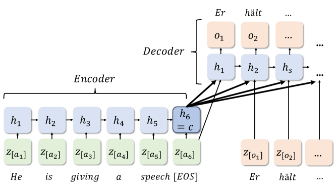
Figure 2: Encoder-Decoder Architecture. Encoder-decoder structure in neural machine translation. In this example, the six token input sentence $(He,is,giving,a,speech,[EOS])$ is translated to German: $($Er, hält, eine, Rede, [EOS]$)$. The end-of-sentence symbol $[EOS]$ is used to signal to the model the end of a sentence. The recurrent encoder processes one input embedding $\bm{z}_{[a_{t}]}$ at a time and updates the input hidden state $\bm{h}_{t}$ at each time step. The last encoder hidden state $\bm{h}_{6}$ serves as context vector $\bm{c}$ that captures all the information from the input sequence. The decoder generates one translated output token at a time. Each output hidden state $\bm{h}_{s}$ is a function of the preceding hidden state $\bm{h}_{s-1}$, the preceding predicted output token embedding $\bm{z}_{[o_{s-1}]}$, and context vector $\bm{c}$.

Another characteristic of early NMT articles is that encoder and decoder are recurrent models (Sutskever et al., 2014, p. 3106) (on recurrent models see Appendix A.3). Hence, the encoder processes each input embedding $\bm{z}_{[a_{t}]}$ step by step. The hidden state at time step $t$, $\bm{h}_{t}$, is a nonlinear function (here denoted by $\sigma$) of the previous hidden state, $\bm{h}_{t-1}$, and input embedding $\bm{z}_{[a_{t}]}$ (Cho et al., 2014, p. 1725):

$$\bm{h}_{t}=\sigma(\bm{h}_{t-1},\bm{z}_{[a_{t}]})$$ (5)

The last encoder hidden state, $\bm{h}_{T}$, corresponds to context vector $\bm{c}$ that then is passed on to the decoder which—given the information encoded in $\bm{c}$—produces a variable-length sequence output $(o_{1},\dots,o_{s},\dots,o_{S})$ (Cho et al., 2014, p. 1725). The decoder also operates in a recurrent manner: Based on the current decoder hidden state $\bm{h}_{s}$, one output token $o_{s}$ is predicted at one time step (Cho et al., 2014, p. 1725). In contrast to the encoder, the hidden state of the decoder at time step $s$, $\bm{h}_{s}$, is not only a function of the previous hidden state $\bm{h}_{s-1}$ but also the embedding of the previous output token $\bm{z}_{[o_{s-1}]}$, and context vector $\bm{c}$ (see also Figure 2) (Cho et al., 2014, p. 1725):

$$\bm{h}_{s}=\sigma(\bm{h}_{s-1},\bm{z}_{[o_{s-1}]},\bm{c})$$ (6)

A problem with this traditional encoder-decoder structure is that all the information about the input sequence—regardless of the length of the input sequence—is captured in a single context vector $\bm{c}$ (Bahdanau et al., 2015, p. 1).

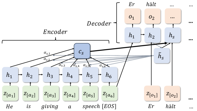
Figure 3: Attention in an Encoder-Decoder Architecture. Visualization of the attention mechanism in an encoder-decoder structure at time step $s$. In the attention mechanism, at each time step, i.e. for each output token, there is a token-specific context vector $\bm{c}_{s}$. $\bm{c}_{s}$ is computed as the weighted sum over all input hidden states $(\bm{h}_{1},\dots,\bm{h}_{6})$. The weights are $(\alpha_{s,1},\dots,\alpha_{s,6})$. $\alpha_{s,1}$ results from a scoring function that captures the similarity between the $s$th output token, as represented by the initial output hidden state $\bm{\tilde{h}}_{s}$, and input token hidden state $\bm{h}_{1}$.

The attention mechanism resolves this problem. In the attention mechanism, at each time step, the decoder can attend to, and thus derive information from, all encoder-produced input hidden states when computing its hidden state $\bm{h}_{s}$ (see Figure 3). More precisely, the decoder hidden state at time point $s$, $\bm{h}_{s}$, is a function of the initial decoder hidden state $\bm{\tilde{h}}_{s}$, the previous output token $\bm{z}_{[o_{s-1}]}$, and an output token-specific context vector $\bm{c}_{s}$ (Luong et al., 2015, p. 1414).

$$\bm{h}_{s}=\sigma(\bm{\tilde{h}}_{s},\bm{z}_{[o_{s-1}]},\bm{c}_{s})$$ (7)

Note that now at each time step there is a context vector $\bm{c}_{s}$ that is specific to the $s$th output token (Bahdanau et al., 2015, p. 3). The attention mechanism rests in the computation of $\bm{c}_{s}$, which is a weighted sum over the input hidden states $(\bm{h}_{1},\dots,\bm{h}_{t},\dots,\bm{h}_{T})$ (Bahdanau et al., 2015, p. 3):

$$\bm{c}_{s}=\sum_{t=1}^{T}\alpha_{s,t}\bm{h}_{t}$$ (8)

The weight $\alpha_{s,t}$ is computed as

$$\alpha_{s,t}=\frac{exp(score(\bm{\tilde{h}}_{s},\bm{h}_{t}))}{\sum_{t^{*}=1}^{T^{*}}exp(score(\bm{\tilde{h}}_{s},\bm{h}_{t^{*}}))}$$ (9)

where $score$ is a scoring function assessing the compatibility between output token representation $\bm{\tilde{h}}_{s}$ and input token representation $\bm{h}_{t}$ (Luong et al., 2015, p. 1414). $score$ could be, for example, the dot product of $\bm{\tilde{h}}_{s}$ and $\bm{h}_{t}$ (Luong et al., 2015, p. 1414). The attention weight $\alpha_{s,t}$ is a measure of the degree of alignment of the $t$th input token, represented by $\bm{h}_{t}$, with the $s$th output token, represented as $\bm{\tilde{h}}_{s}$ (Bahdanau et al., 2015, p. 3-4). Input hidden states that do not match with output token representation $\bm{\tilde{h}}_{s}$ receive a small weight such that their contribution vanishes, whereas input hidden states that are relevant to output token $\bm{\tilde{h}}_{s}$ receive high weights, thereby increasing their contribution (Alammar, 2018c ). Hence, $\bm{c}_{s}$ considers all input hidden states and especially attends to those input hidden states that match with the current output token. As context vector $\bm{c}_{s}$ is constructed for each output token based on a weighted sum of all input hidden states, the attention architecture allows for modeling dependencies between tokens irrespective of their distance (Vaswani et al., 2017, p. 5999).

4.2 The Transformer

The original articles on attention use recurrent architectures in the encoder and decoder. The sequential nature of recurrent models implies that within each training example sequence each token has to be processed one after another—a computationally not efficient strategy (Vaswani et al., 2017, p. 5999). To overcome this inefficiency and to enable parallel processing within training sequences, Vaswani et al., (2017) introduced the Transformer architecture that is built from attention mechanisms. The Transformer consists of a sequence of six encoders followed by a stack of six decoders (see Figure 4) (Vaswani et al., 2017, p. 6000). Each encoder consists of two components: a multi-head self-attention layer (to be explained below) and a feedforward neural network (Vaswani et al., 2017, p. 6000). Each decoder also has a multi-head self-attention layer followed by a multi-head encoder-decoder attention layer and a feedforward neural network (Vaswani et al., 2017, p. 6000). Instead of processing each token of each training example one after another, the Transformer encoder takes as an input the whole set of $T$ embeddings for one training example and processes this set of embeddings, $(\bm{z}_{[a_{1}]},\dots,\bm{z}_{[a_{t}]},\dots,\bm{z}_{[a_{T}]})$, in parallel (Alammar, 2018b ).

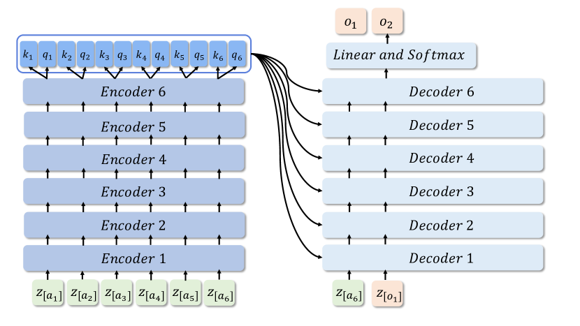
Figure 4: Transformer Architecture. In the original article by Vaswani et al., (2017), the Transformer is made up of a stack of six encoders proceeded by a stack of six decoders. In contrast to recurrent architectures where each input token is handled one after another, a Transformer encoder processes the entire set of input token representations in parallel (Vaswani et al., 2017, p. 5999). Here, the input embeddings are $(\bm{z}_{[a_{1}]},\dots,\bm{z}_{[a_{6}]})$. The sixth encoder passes the key and query vectors of the input tokens, $(\bm{k}_{1},\bm{q}_{1},\dots,\bm{k}_{6},\bm{q}_{6})$, to each of the decoders. These key and query vectors from the last encoder are processed in each decoder’s encoder-decoder attention layer (Vaswani et al., 2017, p. 6002). The Transformer decoders operate in an autoregressive manner, meaning that the stack of decoders processes as an additional input the sequence of previous output tokens (Vaswani et al., 2017, p. 6002). In the visualization here, output tokens are denoted with $(o_{1},o_{2},\dots)$ and the decoder predicts output token $o_{2}$ given the previous tokens $(a_{6},o_{1})$ (where $a_{6}$ is an end-of-sentence symbol). To predict the $t$th output token, the hidden state of the last decoder is processed through a linear layer and a softmax layer to produce a probability distribution over the terms in the vocabulary (Vaswani et al., 2017, p. 6002).

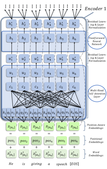
Figure 5: Transformer Encoder Architecture. This visualization details the processes in the first Transformer encoder. The encoder comprises a multi-head self-attention layer and a feedforward neural network, each followed by residual learning and layer normalization. The first encoder takes as an input position-aware embeddings, $(\bm{z}_{[a_{1}]},\dots,\bm{z}_{[a_{6}]})$. (A position-aware embedding is the sum of a pure embedding vector and a positional encoding vector (Vaswani et al., 2017, p. 6003). The positional encoding vector contains information on the position of the $t$th token within the input sequence, thereby making the model aware of token positions (Vaswani et al., 2017, p. 6002-6003).) The position-aware embeddings then are transformed into eight sets of key, query and value vectors. One set is $(\bm{k}_{1},\bm{q}_{1},\bm{v}_{1},\dots,\bm{k}_{6},\bm{q}_{6},\bm{v}_{6})$. These are processed in the multi-head self-attention layer to produce eight sets of context vectors (one set being $(\bm{c}_{1},\dots,\bm{c}_{6})$). The sets then are concatenated and transformed linearly to become the updated representations $(\bm{u}_{1},\dots,\bm{u}_{6})$. After residual learning and layer normalization, $(\bm{u^{*}}_{1},\dots,\bm{u^{*}}_{6})$ enter the feedforward neural network, whose output—after residual learning and layer normalization—are the updated representations produced by the first Transformer encoder: $(\bm{h^{*}}_{1},\dots,\bm{h^{*}}_{6})$. The representations $(\bm{h^{*}}_{1},\dots,\bm{h^{*}}_{6})$ constitute the input to the next encoder, where they are first transformed to sets of key, query and value vectors.

The first element in a Transformer encoder is the multi-head self-attention layer. In the self-attention layer, the provided input sequence $(\bm{z}_{[a_{1}]},\dots,\bm{z}_{[a_{t}]},\dots,\bm{z}_{[a_{T}]})$ attends to itself. Instead of improving the representation of an output token by attending to tokens in the input sequence, the idea of self-attention is to improve the representation of a token $a_{t}$ by attending to the tokens in the same sequence in which $a_{t}$ is embedded in (Alammar, 2018b ). For example, if ‘The company is issuing a statement as it is bankrupt.’ were a sentence to be processed, then the embedding for the token ‘it’ that enters the Transformer would not contain any information regarding which other token in the sentence ‘it’ is referring to. Is it the company or the statement? In the self-attention mechanism, the representation for ‘it’ is updated by attending to—and incorporating information from—other tokens in this sentence (Alammar, 2018b ). It, therefore, is to be expected that after passing through the self-attention layers, the representation of ‘it’ absorbed some of the representation for ‘company’ and so encodes information on the dependency between ‘it’ and ‘company’ (Alammar, 2018b ).

The first operation within a self-attention layer is that each input embedding $\bm{z}_{[a_{t}]}$ is transformed into three separate vectors, called key $\bm{k}_{t}$, query $\bm{q}_{t}$, and value $\bm{v}_{t}$ (see Figure 5). The key, query, and value vectors are three different projections of the input embedding $\bm{z}_{[a_{t}]}$ (Alammar, 2018b ). They are generated by matrix multiplication of $\bm{z}_{[a_{t}]}$ with three different weight matrices, $\bm{W}_{k}$, $\bm{W}_{q}$, and $\bm{W}_{v}$ (Vaswani et al., 2017, p. 6002):

$$\bm{k}_{t}=\bm{z}_{[a_{t}]}\bm{W}_{k}\qquad\bm{q}_{t}=\bm{z}_{[a_{t}]}\bm{W}_{q}\qquad\bm{v}_{t}=\bm{z}_{[a_{t}]}\bm{W}_{v}$$ (10)

Then, for each token $a_{t}$, an updated representation (named context vector $\bm{c}_{t}$) is computed as a weighted sum over the value vectors of all tokens that are in the same sequence as token $a_{t}$ (Vaswani et al.,, 2017, p. 6000-6002):

$$\bm{c}_{t}=\sum_{t^{*}=1}^{T^{*}}\alpha_{t,t^{*}}\bm{v}_{t^{*}}$$ (11)

The attention weight $\alpha_{t,t^{*}}$ is a function of the similarity between token $a_{t}$, represented by $\bm{q}_{t}$, and token $a_{t^{*}}$, that is represented as $\bm{k}_{t^{*}}$:

$$\alpha_{t,t^{*}}=\frac{exp(score(\bm{q}_{t},\bm{k}_{t^{*}}))}{\sum_{t^{*}=1}^{T^{*}}exp(score(\bm{q}_{t},\bm{k}_{t^{*}}))}$$ (12)

where $score$ is $(\bm{q}_{t}\bm{k}_{t^{*}}^{\top})/\sqrt{|\bm{k}_{t^{*}}|}$ (Vaswani et al., 2017, p. 6001). $\alpha_{t,t^{*}}$ indicates the contribution of token $a_{t^{*}}$ for the representation of token $a_{t}$. Thus, attention vector $\bm{c}_{t}$ is calculated as in a basic attention mechanism (see Equations 8 and 9)—except that the attention now is with respect to the value vectors of the tokens that are part of the same sequence as $a_{t}$ (see also Figure 6).

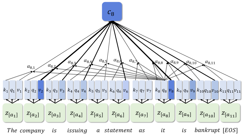
Figure 6: Attention Mechanism in the Transformer. Illustration of the attention mechanism in the first Transformer encoder for the $8$th token (‘it’) in the example sentence ‘The company is issuing a statement as it is bankrupt.’. The arrows pointing from the value vectors $(\bm{v}_{1},\dots,\bm{v}_{11})$ to context vector $\bm{c}_{8}$ are the weights $(\alpha_{8,1},\dots,\alpha_{8,t^{*}},\dots,\alpha_{8,11})$. A single weight $\alpha_{8,t^{*}}$ indicates the contribution of token $t^{*}$ to the representation of token $8$, $\bm{c}_{8}$. The larger $\alpha_{8,t^{*}}$ is assumed to be in this example, the thicker the arrow and the darker the corresponding value vector. The dotted lines symbolize the computation of the weights $(\alpha_{8,1},\dots,\alpha_{8,t^{*}},\dots,\alpha_{8,11})$.

The self-attention mechanism outlined so far is conducted eight times in parallel (Vaswani et al., 2017, p. 6001-6002). Hence, for each token $a_{t}$, eight different sets of query, key and value vectors are generated and there will be not one but eight attention vectors $\{\bm{c}_{t,1},\dots,\bm{c}_{t,8}\}$ (Vaswani et al., 2017, p. 6001-6002). In doing so, each attention vector can attend to different tokens in each of the eight different representation spaces (Vaswani et al., 2017, p. 6002). For example, in one representation space the attention vector for token $a_{t}$ may learn syntactic structures and in another representation space the attention vector may attend to semantic connections (Vaswani et al., 2017, p. 6004; Clark et al., 2019). Because the self-attention mechanism is implemented eight times in parallel and generates eight attention vectors (or heads), the procedure is called multi-head self-attention (Vaswani et al., 2017, p. 6001). The eight attention vectors subsequently are concatenated into a single vector, $\bm{c}_{t}=[\bm{c}_{t,1};\dots;\bm{c}_{t,8}]$, and multiplied with a corresponding weight matrix $\bm{W}_{0}$ to produce vector $\bm{u}_{t}$ (Vaswani et al., 2017, p. 6002): $\bm{u}_{t}=\bm{c}_{t}\bm{W}_{0}$. Afterward, $\bm{u}_{t}$ is added to $\bm{z}_{[a_{t}]}$, thereby allowing for residual learning (He et al., 2015). Then, layer normalization as suggested in Ba et al., (2016) is conducted (Vaswani et al., 2017, p. 6000).

$$\bm{u^{*}}_{t}=LayerNorm(\bm{u}_{t}+\bm{z}_{[a_{t}]})$$ (13)

$\bm{u^{*}}_{t}$ then enters a feedforward neural network with a Rectified Linear Unit (ReLU) activation function (Vaswani et al., 2017, p. 6002)

$$\bm{h}_{t}=max(0,\bm{u^{*}}_{t}\bm{W}_{1}+\bm{b}_{1})\bm{W}_{2}+\bm{b}_{2}$$ (14)

followed by a residual connection with layer normalization (Vaswani et al., 2017, p. 6000):

$$\bm{h^{*}}_{t}=LayerNorm(\bm{h}_{t}+\bm{u^{*}}_{t})$$ (15)

$\bm{h^{*}}_{t}$ finally is the representation of token $a_{t}$ produced by the encoder. It constitutes an updated representation of input embedding $\bm{z}_{[a_{t}]}$. Due to the self-attention mechanism, $\bm{h^{*}}_{t}$ is a function of the other tokens in the same sequence and thus captures context-dependent information. Hence, $\bm{h^{*}}_{t}$ is a contextualized representation of token $a_{t}$. The same token in another sequence would obtain another token representation vector.

The entire sequence of representations, $(\bm{h^{*}}_{1},\dots,\bm{h^{*}}_{t},\dots,\bm{h^{*}}_{T})$, that is produced as the encoder output, serves as the input for the next encoder that generates eight sets of query, key, and value vectors from each representation $\bm{h^{*}}_{t}$ to implement multi-head self attention and to finally produce an updated set of representations, $(\bm{h^{*}}_{1},\dots,\bm{h^{*}}_{t},\dots,\bm{h^{*}}_{T})^{*}$, that are passed to the next encoder and so on. The last encoder from the stack of encoders passes the key and value vectors from its produced sequence of updated representations to each encoder-decoder multi-head attention layer in each decoder (see Figure 4) (Vaswani et al., 2017, p. 6002). Except for the encoder-decoder attention layer in which the decoder pays attention to the encoder input, the architecture of each decoder is largely the same as those of the encoders (Vaswani et al., 2017, p. 6000). Note, however, that the stack of decoders operates in an autoregressive manner (Vaswani et al., 2017, p. 5999). This is, when making the prediction for the next output token $o_{s}$, the decoders have access to and process the sequence of previous output tokens, $(a_{T},o_{s},\dots,o_{s-1})$, as additional inputs (see Figure 4) (Vaswani et al., 2017, p. 5999). In order to ensure that the decoders are autoregressive, self-attention in each decoder is masked, meaning that the attention vector for output token $o_{s}$ can only attend to output tokens preceding token $o_{s}$ (Vaswani et al., 2017, p. 6000). To predict an output token, the hidden state of the last decoder is handed to a linear and softmax layer to produce a probability distribution over the vocabulary (Vaswani et al., 2017, p. 6002).

5 Transfer Learning with Transformer-Based Models

Taken together, the Transformer architecture in combination with transfer learning literally transformed the field of NLP (Bommasani et al., 2021, p. 5). After the introduction of the Transformer by Vaswani et al., (2017), several models for transfer learning that included elements of the Transformer were developed (e.g. Radford et al., 2018; Devlin et al., 2019; Yang et al., 2019; Clark et al., 2020; Raffel et al., 2020). These models and their derivatives significantly outperformed previous state-of-the-art models.

An important step within these developments was the introduction of BERT (Devlin et al., 2019). By establishing new state-of-the-art performance levels for eleven NLP tasks, BERT demonstrated the power of transfer learning (Bommasani et al., 2021, p. 5). The introduction of BERT finally paved the way to a new transfer learning-based mode of learning in which it is common to use an already pretrained language model and adapt it to a specific target task as needed (Alammar, 2018a ; Bommasani et al., 2021, p. 5). Simultaneously with and independently of BERT, a wide spectrum of Transformer-based models for transfer learning have been developed. This section first introduces BERT and then provides an overview of further models.

5.1 BERT

BERT consists of a stack of Transformer encoders and comes in two different model sizes (Devlin et al., 2019, p. 4173): BERT_BASE consists of 12 stacked Transformer encoders, each with 12 attention heads. The dimensionality of the input embeddings and the updated hidden vector representations is 768. BERT_LARGE has 24 Transformer encoders with 16 attention heads and a hidden vector size of 1024. As in the original Transformer, the first BERT encoder takes as an input a sequence of embedded tokens, $(\bm{z}_{[a_{1}]},\dots,\bm{z}_{[a_{t}]},\dots,\bm{z}_{[a_{T}]})$, processes the embeddings in parallel through the self-attention layer and the feedforward neural network to generate a set of updated token representations, $(\bm{h^{*}}_{1},\dots,\bm{h^{*}}_{t},\dots,\bm{h^{*}}_{T})$, that are then passed to the next encoder that also generates updated representations to be passed to the next encoder and so on until the representations finally enter output layers for prediction (Alammar, 2018a ).

The authors inventing BERT sought to tackle a disadvantage of the classic language modeling pretraining task (see Equations 3 and 4), namely that it is strictly unidirectional (Devlin et al., 2019, p. 4171). A forward language model can only access information from the preceding tokens $(a_{1},\dots,a_{t-1})$ but not from the following tokens $(a_{t+1},\dots,a_{T})$. The same is true for a backward language model in which information can only be captured from succeeding tokens (Yang et al., 2019, p. 5753). Assuming that a representation of token $a_{t}$ from a bidirectional model that simultaneously can attend to preceding and succeeding tokens may constitute a better representation of token $a_{t}$ than a representation stemming from a unidirectional language model, the authors of BERT invented an adapted variant of the traditional language modeling pretraining task, named masked language modeling, to learn deep contextualized representations that are bidirectional (Devlin et al., 2019, p. 4171-4172).

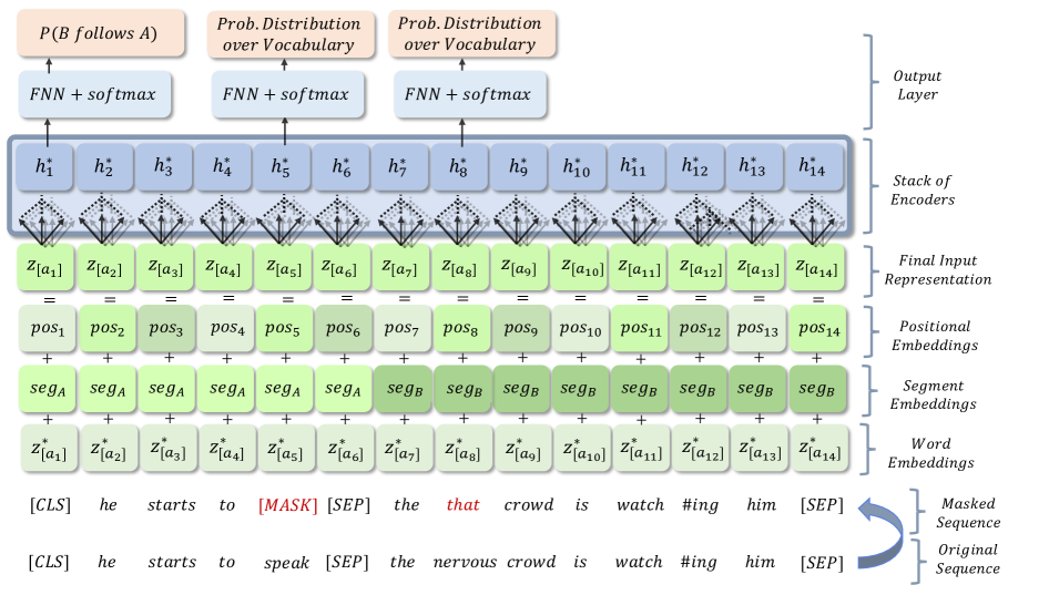
Figure 7: Pretraining BERT. Architecture of BERT in pretraining. Assume that in the lowercased example sequence consisting of the segment pair ‘he starts to speak. the nervous crowd is watch-ing him.’ the tokens ‘speak’ and ‘nervous’ were sampled to be masked. ‘speak’ is replaced by the ‘[MASK]’ token and ‘nervous’ is replaced by the random token ‘that’. The model’s task is to predict the tokens ‘speak’ and ‘nervous’ from the representation vectors it learns at the positions of the input embeddings of ‘[MASK]’ and ‘that’. $P(BfollowsA)$ is the next sentence prediction task. FNN stands for feedforward neural network.

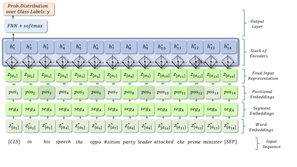
Figure 8: Fine-Tuning BERT. Architecture of BERT during fine-tuning on a single sequence classification task.

To conduct the masked language modeling task in the pretraining process of BERT, in each input sequence, $15\%$ of the input embeddings are selected at random (Devlin et al., 2019, p. 4174, 4183). The selected tokens are indexed as $(1,\dots,q,\dots,Q)$ here. $80\%$ of the $Q$ selected tokens will be replaced by the ‘[MASK]’ token (Devlin et al., 2019, p. 4174). $10\%$ of the selected tokens are supplanted with another random token, and $10\%$ of selected tokens remain unchanged (Devlin et al., 2019, p. 4174). The task then is to correctly predict all $Q$ tokens sampled for the task based on their respective input token representation (for an illustration see Figure 7) (Devlin et al., 2019, p. 4173-4174). In doing so, self-attention is possible with regard to all—instead of only preceding or only succeeding—tokens in the same sequence, and thus the learned representations for all tokens in the sequence can capture encoded information from bidirectional contexts (Devlin et al., 2019, p. 4174, 4182).

In addition to the masked language modeling task, BERT is also pretrained on a next sentence prediction task in which the model has to predict whether the second of two text segments it is presented with succeeds the first (Devlin et al., 2019, p. 4172, 4174). The second pretraining task is hypothesized to serve the purpose of making BERT also a well-generalizing pretrained model for NLP target tasks that require an understanding of the association between two text segments (e.g. question answering or natural language inference) (Devlin et al., 2019, p. 4172, 4174).

To accommodate for the pretraining tasks and to prepare for a wide spectrum of downstream target tasks, the input format accepted by BERT consists of the following elements (see Figure 7) (Devlin et al., 2019, p. 4174-4175, 4182-4183):

• Each sequence of tokens $(a_{1},\dots,a_{t},\dots,a_{T})$ is set to start with the classification token ‘[CLS]’. After fine-tuning, the ‘[CLS]’ token functions as an aggregate representation of the entire sequence and is used as an input for single sequence classification target tasks such as sentence sentiment analysis.

• The separation token ‘[SEP]’ is used to separate different segments.

• Each token $a_{t}$ is represented by the sum of its input embedding with a positional embedding and a segment embedding.

• In software-based implementations, BERT-like models typically require all input sequences to have the same length (Hugging Face, 2020a ). To meet this requirement, the text sequences are tailored to the same length by padding or truncation (Hugging Face, 2020a ). Truncation is employed if text sequences exceed the maximum accepted sequence length. Truncation implies that excess tokens are removed. In padding, a padding token (‘[PAD]’) is repeatedly added to a sequence until the desired length is reached (McCormick & Ryan, 2019). Note that due to memory restrictions, the maximum sequence length that BERT can process is limited to 512 tokens.

BERT is pretrained with the masked language modeling and the next sentence prediction task. As pretraining corpora the BooksCorpus (Zhu et al., 2015) and the English Wikipedia are used (Devlin et al., 2019, p. 4175). Taken together the pretraining corpus consists of $3.3$ billion tokens (Devlin et al., 2019, p. 4175). (For details on pretraining BERT see Appendix D.)

Token representations that are produced from a pretrained BERT model afterward can be extracted and taken as an input for a target task-specific architecture as in a classic feature extraction approach (Devlin et al., 2019, p. 4179). The more common way to use BERT, however, is to fine-tune BERT on the target task. Here, merely the output layer from pretraining is exchanged with an output layer tailored for the target task (Devlin et al., 2019, p. 4173, 4184). Other than that, the same model architecture is used in pretraining and fine-tuning (compare Figures 7 and 8) (Devlin et al., 2019, p. 4173, 4184). If the target task is to classify single input sequences into a set of predefined categories (see Figure 8), the hidden state vector generated by the last Transformer encoder for the [CLS] token, $\bm{h}^{*}_{1}$, enters the following output layer to generate output vector $\bm{y}$ (Hugging Face, 2018):

$$\bm{y}=softmax(\tanh(\bm{h}^{*}_{1}\bm{W}_{1}+\bm{b}_{1})\bm{W}_{2}+\bm{b}_{2})$$ (16)

$\bm{y}$’s dimensionality corresponds to $C$—the number of categories in the target classification task. The $c$th element of $\bm{y}$ gives the predicted probability of the input sequence belonging to the $c$th class. During fine-tuning, not only the weight matrices and bias terms in Equation 16 but all parameters of BERT are updated (Devlin et al., 2018, p. 6).

5.2 More Transformer-Based Pretrained Models

A helpful way to describe and categorize the various Transformer-based models for transfer learning is to differentiate them according to their pretraining objective and their model architecture (Hugging Face, 2020b ). The major groups of models in this categorization scheme are autoencoding models, autoregressive models, and sequence-to-sequence models (Hugging Face, 2020b ).

5.2.1 Autoencoding Models

In their pretraining task, autoencoding models are presented with input sequences that are altered at some positions (Yang et al., 2019, p. 5753-5755). The task is to correctly predict the uncorrupted sequence (Yang et al., 2019, p. 5753-5755). The models’ architecture is typically composed of the encoders of the Transformer which implies that autoencoding models can access the entire set of input sequence tokens and can learn bidirectional token representations (Hugging Face, 2020b ). Autoencoding models tend to be especially high performing in sequence or token classification target tasks (Hugging Face, 2020b ). BERT with its masked language modeling pretraining task is a typical autoencoding model (Yang et al., 2019, p. 5753).

Among the various extensions of BERT that have been developed since its introduction, RoBERTa (Liu et al., 2019) is widely known. RoBERTa makes changes in the pretraining and hyperparameter settings of BERT. For example, RoBERTa is only pretrained on the masked language modeling and not the next sentence prediction task (Liu et al., 2019, p. 4-6). Masking is performed dynamically each time before a sequence is presented to the model instead of being conducted once in data preprocessing (Liu et al., 2019, p. 4, 6). Moreover, RoBERTa is pretrained on more data and more heterogeneous data (e.g. also on web corpora) (Liu et al., 2019, p. 5-6).

One major disadvantage of pretrained models that are based on the self-attention mechanism in the Transformer is that currently available hardware does not allow Transformer-based models to process long text sequences (Beltagy et al., 2020, p. 1). The reason is that the memory and time required increase quadratically with sequence length (Beltagy et al., 2020, p. 1). Long text sequences thereby quickly exceed memory limits of presently existing graphics processing units (GPUs) (Beltagy et al., 2020, p. 1). Transformer-based pretrained models therefore typically induce a maximum sequence length. For BERT and related models this maximum length usually is 512 tokens. Simple workarounds for processing sequences longer than 512 tokens (e.g. truncating texts or processing them in chunks) lead to information loss and potential errors (Beltagy et al., 2020, p. 2-3). To solve this problem, various works present procedures for altering the Transformer architecture such that longer text documents can be processed (Child et al., 2019; Dai et al., 2019; Beltagy et al., 2020; Kitaev et al., 2020; Wang et al., 2020; Zaheer et al., 2020).

Here, one of these models, the Longformer (Beltagy et al., 2020), is presented in more detail. The Longformer introduces a new variant of the attention mechanism such that time and memory complexity does not scale quadratically but linearly with sequence length and thus longer texts can be processed (Beltagy et al., 2020, p. 3). The attention mechanism in the Longformer is composed of a sliding window as well as global attention mechanisms for specific preselected tokens (Beltagy et al., 2020, p. 3-4). In the sliding window, each input token $a_{t}$—instead of attending to all tokens in the sequence—attends only to a fixed number of tokens to the left and right of $a_{t}$ (Beltagy et al., 2020, p. 3). In order to learn representations better adapted to specific NLP tasks, the authors use global attention for specific tokens on specific tasks (e.g. for the ‘[CLS]’ token in sequence classification tasks) (Beltagy et al., 2020, p. 3-4). These preselected tokens directly attend to all tokens in the sequence and enter the computation of the attention vectors of all other tokens (Beltagy et al., 2020, p. 3-4). The Longformer allows processing text sequences of up to 4,096 tokens (Beltagy et al., 2020, p. 6). This Longformer-specific attention mechanism can be used as a plug-in replacement of the original attention mechanism in any Transformer-based model (Beltagy et al., 2020, p. 6). Beltagy et al., (2020, p. 2) insert the Longformer attention mechanism into the RoBERTa architecture and then continue to pretrain RoBERTa with the Longformer attention mechanism on the masked language modeling task (Beltagy et al., 2020, p. 2).

5.2.2 Autoregressive Models

Autoregressive models are pretrained on the classic language modeling task (see Equations 3 and 4) (Yang et al., 2019, p. 5753-5755). They are trained to predict the next token given all the preceding tokens in a sequence, $P(a_{t}|a_{1},\dots,a_{t-1})$, and/or to predict the next token given all succeeding tokens, $P(a_{t}|a_{T},\dots,a_{t+1})$ (Yang et al., 2019, p. 5753). Hence, autoregressive models are not capable of learning genuine bidirectional representations that draw from left and right contexts (Yang et al., 2019, p. 5753). In correspondence with this pretraining objective, their architecture is typically based only on the decoders of the Transformer (without encoder-decoder attention) (Hugging Face, 2020b ). Due to their decoder-based architecture and the characteristics of their pretraining task, autoregressive models are typically very good at target tasks in which they have to generate text (Hugging Face, 2020b ). Autoregressive models, however, can be successfully fine-tuned to a large variety of downstream tasks (Hugging Face, 2020b ). An elementary autoregressive model is the GPT (Radford et al., 2018). Its successors GPT-2 (Radford et al., 2019) and GPT-3 (Brown et al., 2020) are well-known and also play a role in the context of zero-shot learning (see Appendix B). Another model using the autoregressive language modeling framework is the XLNet (Yang et al., 2019). (On the XLNet see Appendix F).

5.2.3 Sequence-to-Sequence Models

The architecture of sequence-to-sequence models contains Transformer encoders and decoders (Hugging Face, 2020b ). They tend to be pretrained on sequence-to-sequence tasks (e.g. translation) and, consequently, are especially suited for sequence-to-sequence-like downstream tasks such as translating or summarizing input sequences (Hugging Face, 2020b ). The Transformer itself is a sequence-to-sequence model for translation tasks. BART (Lewis et al., 2020) and the T5 (Raffel et al., 2020) are further well-known sequence-to-sequence models applicable to a large variety of target tasks (Hugging Face, 2020b ). (On the T5 and BART see Appendix G.)

5.3 Foundation Models: Concept, Limitations, and Issues

Whilst this article focuses on transfer learning with Transformer-based models in the context of text classification tasks for the purpose of measurement, the application of transfer learning as a mode of learning, as well as the application of the Transformer as a deep neural network architecture, is not restricted to classification tasks, text data, or the purpose of measurement. Porter & Velez, (2021), for example, apply the GPT-2 to generate placebos texts in social science survey experiments. Moreover, transfer learning and the Transformer architecture are at the heart of fundamental changes within the entire field of NLP and beyond: AI research previously had moved from classic machine learning (in which a function between representations of data and outputs are learned but representations still have to be engineered) to the era of deep learning (in which deep neural networks learn representations of data but still typically one model is trained for one specific task) (Bommasani et al., 2021, p. 3-4). Now, AI research seems to move toward the widespread use of pretrained deep neural networks that function as highly general all-purpose models (Bommasani et al., 2021, p. 3-6). Such deep neural networks that are pretrained in a self-supervised fashion on large amounts of data and then can be adapted to a wide spectrum of target tasks are also called foundation models (Bommasani et al., 2021). During the last few years, foundation models not only have taken hold in NLP but across the field of AI research (Bommasani et al., 2021). Thus, transfer learning with (Transformer-based) deep neural networks is not only applied to text data but also, for example, to images (Dosovitskiy et al., 2021; Goyal et al., 2021), videos (Sun et al., 2019a ), audio data (Baevski et al., 2020), and data in tabular form (Yin et al., 2020). Moreover, an increasing number of models are multimodal (e.g. Bapna et al., 2021; Fu et al., 2021; Radford et al., 2021; Ramesh et al., 2021). Summarizing current developments, the emerging mode of learning is characterized by a deep neural network that

• is frequently based on the Transformer architecture.

• has been pretrained—typically in self-supervised learning mode—on massive amounts of data from various sources and domains. (Pretraining does not have to be constrained to one pretraining task conducted on one type of data in one language. Rather, increasingly general models are developed by pretraining on multiple tasks (Wei et al., 2022; Aribandi et al., 2022), pretraining on data in multiple languages (Conneau et al., 2020; Babu et al., 2021), or pretraining on data from multiple modes (Luo et al., 2020; Bapna et al., 2021; Radford et al., 2021).)

• can process—and learn representations for—these data inputs (probably across domains, languages, and modes) (Tenney et al., 2019a ; Radford et al., 2021),

• after adaptation can be applied to a wide spectrum of tasks, for example, various language understanding tasks (Devlin et al., 2019; Liu et al., 2019), different language understanding plus language generation tasks (Lewis et al., 2020; Wei et al., 2022), or tasks related to the understanding and/or generation of data in multiple modes (Luo et al., 2020; Fu et al., 2021; Ramesh et al., 2021).

Foundation models have triggered significant performance enhancements but also come with substantive limitations and problematic issues. One major concern, for example, is that the amounts of resources required in pretraining (especially in terms of data and compute) are so massively large that academic institutions and the scientific research community struggle (or are not able) to pretrain the largest foundation models (but see https://bigscience.huggingface.co/) (Bommasani et al., 2021, p. 11). Moreover, the data used in pretraining and the model source code are not always publicly available (Aßenmacher & Heumann, 2020, p. 4; Riedl, 2020). This raises deep concerns regarding accessibility and traceability. Another problematic aspect is that these models reflect the representational biases (e.g. stereotypes, underrepresentations) encoded in the data they have been pretrained on (Bommasani et al., 2021, p. 129-131). As soon as a model is adapted to some target task, these biases can materialize with serious negative consequences (Bommasani et al., 2021, p. 130). A further problem is the fixed (typically relatively small) maximum sequence length that Transformer-based models can process. Whatever the given current computational restrictions, efficient modifications of the self-attention mechanism, as for example presented by the Longformer (Beltagy et al., 2020), allow for longer sequences to be processed than with the original Transformer and thereby constitute important steps toward alleviating this major drawback.

Besides these issues related to large pretrained representation models, the mere application of deep neural networks is likely to pose further difficulties for social science researchers. One issue is interpretability: If a researcher applies a learning method to measure an a priori-defined concept from text, the ability to as closely as possible imitate human codings on yet unseen test data is arguably the most important goal because this ability indicates the measure’s validity. In this very context, a model’s prediction performance thus is considered more important than a model’s interpretability. Yet interpretability (i.e. the human-understandable and accurate representation of a model’s decision process) can be highly important (Miller, 2019; Jacovi & Goldberg, 2020). Interpretability makes a model’s predictions more transparent and more human-retraceable. If a researcher can understand why a model made predictions in a particular way and if a researcher can estimate the effect of input features for a model’s predictions, this can enhance the researcher’s trust in the model she applies (Doshi-Velez & Kim, 2017, p. 2; Molnar, 2022, ch. 3.1). Because deep neural networks do not operate on a priori-defined, human-engineered features but have a layered architecture that enables them to learn complex representations of textual inputs, interpretation of deep neural networks is less straightforward and neural network-specific interpretation methods tend to be used (Belinkov & Glass, 2019, p. 49; Molnar, 2022, ch. 10). (For an overview of common methods to make neural networks interpretable see Appendix H.) The open-source library Captum (https://captum.ai/) is likely to be a useful interpretability tool. Captum implements several attribution algorithms that allow researchers to examine how predicted outputs relate to input features (Kokhlikyan et al., 2020, p. 3). Captum furthermore provides tools for analyzing attention patterns (see https://captum.ai/tutorials/Bert˙SQUAD˙Interpret2).

Another issue is reproducibility: As for conventional models, reproducibility issues with deep neural networks typically arise from random elements that are used during optimization and/or when sampling data (e.g. in cross-validation, or batch allocation). In both cases, sources of randomness usually can be controlled. Yet in practice, this often proves to be more difficult for deep neural networks than for conventional models. Note, furthermore, that full reproducibility across different computing platforms and environments cannot be ensured (Freidank, 2020; Torch Contributors, 2021).

6 Applications

Researchers who wish to apply sequential transfer learning can pretrain a model on a suitable source task by themselves and then finetune the pretrained model to their target task of interest. Because pretraining tends to be very expensive, however, the much more convenient, cost-effective, and common approach for applied researchers is to make use of an already pretrained model and then to merely adapt the pretrained model to the target task. Hence, to fully leverage the power of neural transfer learning, researchers require access to already pretrained models that they can fine-tune on their specific tasks. Such access is provided by Hugging Face’s Transformers (Wolf et al., 2020) which is an open-source library that contains thousands of pretrained NLP models ready to download and use: https://huggingface.co/. The Hugging Face library contains pretrained versions of the models discussed here and a great many models more. Most of the available pretrained models in the Hugging Face library have been pretrained on English texts, yet there are numerous monolingual models pretrained in other languages. Moreover, the library also comprises several models for cross-lingual learning that have been pretrained on text in several languages. The pretrained models can be accessed via the respective Transformers Python package that also provides compatibility with PyTorch (Paszke et al., 2019) and TensorFlow (Abadi et al., 2016).

In the applications presented in the following neural transfer learning is conducted in Python 3 (van Rossum & Drake, 2009) making use of PyTorch (Paszke et al., 2019) and pretrained models from Hugging Face’s Transformers (Wolf et al., 2020). The code is executed in Google Colab. Whenever a GPU is used, an NVIDIA Tesla T4 is employed. The source code for this study is openly available in figshare at https://doi.org/10.6084/m9.figshare.14394173. Especially the shared Colab Notebooks serve as templates that other researchers can easily adapt for their NLP tasks.

6.1 Models, Data Sets, and Tasks

The aim of this applied section is to explore the use of transfer learning with Transformer-based models for text analyses in social science contexts. To do so, the prediction performances of BERT, RoBERTa, and the Longformer are compared to the performances of two conventional machine learning algorithms: Support vector machines (SVMs) (Boser et al., 1992; Cortes & Vapnik, 1995) and the gradient tree boosting algorithm XGBoost (Chen & Guestrin, 2016). SVMs have been widely used in social science text applications (e.g. Diermeier et al., 2011; D’Orazio et al., 2014; Ramey et al., 2019; Miller et al., 2020; Sebők & Kacsuk, 2021). As a tree-based (boosting) method XGBoost represents a type of algorithm also commonly utilized (e.g. Katagiri & Min, 2019; Anastasopoulos & Bertelli, 2020; Park et al., 2020). The comparisons are conducted on the basis of three different data sets of varying sizes and textual styles:

1. The Ethos Dataset (Duthie & Budzynska, 2018) is a corpus of 3,644 sentences from debates in the UK parliament (train: 2,440; test: 1,204). Duthie & Budzynska, (2018) gathered 90 debate transcripts from the period Margaret Thatcher served as Prime Minister (1979-1990). In each debate, they recorded for each spoken sentence whether the sentence refers to the ethos (i.e. the character) of another politician or party, and if so whether the other’s ethos is supported or attacked (Duthie & Budzynska, 2018, p. 4042). The task associated with this data set thus is to as precisely as possible measure the concept of ethos from text. With $82.5\%$ of the sentences being non-ethotic, $12.9\%$ attacking and $4.6\%$ supporting another’s ethos, the data are quite imbalanced.

2. The Legalization of Abortion Dataset comprises 933 tweets (train: 653; test: 280). The data set is a subset of the Stance Dataset (Mohammad et al., 2017) that was used for detecting the attitude toward five different targets from tweets. Mohammad et al., (2017) collected the tweets via hashtags and let CrowdFlower workers annotate the tweets regarding whether the tweeter is in favor, against, or neutral toward the target of interest (Mohammad et al., 2017, p. 4-7). The Legalization of Abortion Dataset used here contains those tweets that refer to the target ‘legalization of abortion’. The task associated with this data set thus is to measure attitudes toward a policy issue from text. $58.3\%$ of the tweets express an opposing and $17.9\%$ a favorable position toward legalization of abortion whilst $23.8\%$ express a neutral or no position.

3. The Wikipedia Toxic Comment Dataset (Jigsaw/Conversation AI, 2018) contains 159,571 comments from Wikipedia Talk pages that were annotated by human raters for their toxicity. On Wikipedia Talk pages contributors discuss changes to Wikipedia pages and articles. Toxic comments are comments that are obscene, threatening, insulting, or express hatred toward social groups and identities (Jigsaw/Conversation AI, 2018). The task here is to separate toxic from non-toxic comments. Tasks in which the aim is to separate documents in which a concept (here: toxicity) occurs from documents in which the concept does not occur are common in text-based social science applications. Such tasks often constitute a first step in a text analysis in which documents that refer to concepts or entities that are of interest to the analysis have to be singled out from a large heterogeneous corpus (Wankmüller, 2022). Frequently, such tasks are imbalanced classification problems (Manning et al., 2008, p. 155). Here, $9.6\%$ of the comments in the data are toxic. The Wikipedia Toxic Comment Dataset is used to assess in how far the algorithms’ performances vary with training set size. To do so, five training data sets of sizes 10,000, 5,000, 2,000, 1,000, and 500 and a test set comprising 1,000 comments are sampled uniformly at random from the 159,571 comments in the Wikipedia Toxic Comment Dataset. To account for the uncertainty induced by operating on samples of training sets, five iterations are performed. This is, the sampling is repeated five times, such that there are five sets comprising five training data sets of varying sizes.

The three applications—Ethos, Abortion, and Toxic—are selected so that the methods are applied on text data that, on the one hand, represent types of texts that are often used within social science and, on the other hand, vary regarding core characteristics (for a comparison see also Figures 9a to 9i). Across the three applications, textual style ranges from the formal, rule-based, courteous language of parliamentary speeches over the short, statement-like nature of tweets to informal, interrelating (and at times disrespectful) comments from online discussions (to get an impression see the most frequent trigrams in Figures 9c, 9f, 9i). The tasks associated with the applications vary with regard to the number of class labels (binary vs. three-class classification) and the distribution over these labels (see Figures 9a, 9d, 9g). The data sets are furthermore characterized by different document lengths (see Figures 9b, 9e, 9h) and vary with regard to their sizes (and hence the number of data available for training).

Ethos	Abortion	Toxic
9a:	9d:	9g:
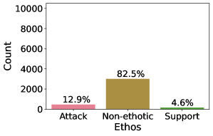
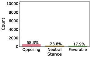
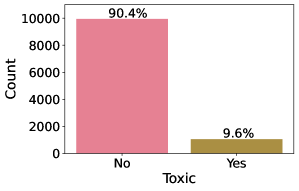
9b:	9e:	9h:
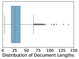
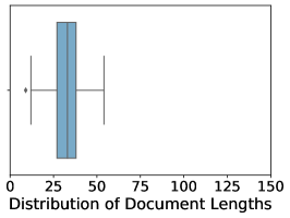
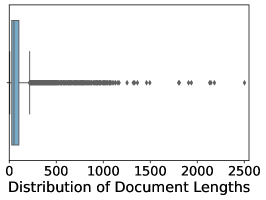
9c:	9f:	9i:

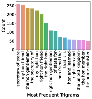
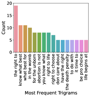
Figure 9: Description of the Corpora. Figures 9a-9c: Ethos Datatset. Figures 9d-9f: Legalization of Abortion Dataset. Figures 9g-9i: Sample of 11,000 comments from the Wikipedia Toxic Comment Dataset. Figures 9a-9g: Class label distributions. Figures 9b-9h: Boxplots visualizing the distribution of the number of tokens per document. Figures 9c-9i: Most frequent trigrams. If possible and reasonable, the figures’ axes have the same scale.

The fewer training data, the more class labels, and the more imbalanced the distribution over class labels, the more difficult a task is likely to be. Especially with regard to imbalanced classification problems when the proportion of training instances in the minority class is small, it can be difficult to have enough training data to train an adequately performing deep neural network from scratch. As transfer learning reduces the number of required training instances, transfer learning is likely to facilitate the training of neural networks in situations of imbalance. Nevertheless, random oversampling is additionally applied here (see Section 6.4 below).

6.2 Text Preprocessing for the Conventional Models

Two types of preprocessing procedures are employed on the raw texts to provide data representation inputs for the conventional models SVM and XGBoost:

1. Basic BOW: The texts are tokenized into unigrams. Punctuation, numbers, and symbols are removed in the Ethos application but kept in the other applications. Afterward, the tokens are lowercased and stemmed. Then, tokens occurring in less than a tiny share of documents (e.g. $0.1\%$ in the Ethos application) and more than a large share of documents (e.g. $33\%$ in the Ethos application) are excluded. Finally, the elements in the document-feature matrix are weighted such that the mere presence (1) vs. absence (0) of each feature within each document is recorded.

2. GloVe Representation: For each unigram that occurs at least 3 (Ethos, Abortion) or 5 (Toxic) times in the respective corpus, the 300-dimensional pretrained GloVe word vector is identified (Pennington et al., 2014). Each document then is represented by the mean over its unigrams’ GloVe word vectors. Due to making use of pretrained feature representations that are not updated during training, GloVe Representation constitutes a transfer learning approach with feature extraction. By averaging over the unigrams’ word embeddings, the word order, however, is not taken into account.

6.3 Text Preprocessing for the Transformer-Based Models

Before the Transformer-based models are applied, the documents are transformed to the required input format. In each document, the tokens are lowercased and the special ‘[CLS]’ and ‘[SEP]’ tokens are added. Then, each token is converted to an index identifying its input embedding and is associated with an index identifying its segment embedding. Additionally, each document is padded to the same length. In the Ethos and Legalization of Abortion corpora, this length corresponds to the maximum document length among the training set documents, which is $139$ and $54$ tokens respectively. The comments from Wikipedia Talk pages pose a problem here: An inspection of the distribution of sequence lengths in the sampled subsets of the Wikipedia Toxic Comment Dataset (see Figure 9h) shows that the vast majority of comments are shorter than the maximum number of $512$ tokens that BERT and RoBERTa can distinguish—but there is a long tail of comments exceeding $512$ tokens. To address this issue, two different approaches are explored: For BERT, following the best strategy identified by Sun et al., 2019b , in each comment that is longer than 512 tokens, only the first 128 and the last 382 tokens are kept while the tokens positioned in the middle are removed. RoBERTa, in contrast, is replaced with the Longformer in the Toxic application. For the Longformer the sequence length is set to $2*512=$ 1,024 tokens. This ensures that in each run only a small one- or two-digit number of sequences that are longer than 1,024 tokens are truncated by removing tokens from the middle whilst padding the texts to a shared length that still can be processed with given memory restrictions.

6.4 Training on the Target Tasks

Pretrained BERT, RoBERTa and Longformer models are accessed from the Hugging Face’s Transformers library (https://huggingface.co/) and then are adapted to each of the target tasks. When doing so, the Adam algorithm as introduced by Loshchilov & Hutter, (2019) with a linearly decaying global learning rate, no warmup, and no weight decay is employed. Dropout is set to $0.1$. To fine-tune the models within the memory resources provided by Colab, small batch sizes are used. In the Ethos and Abortion applications, a batch size of $16$ is selected. A batch in the Toxic application comprises $8$ (and for the Longformer $4$) text instances. Moreover, for the pretrained models, the base size of the model architecture is used instead of the large or extra large model versions. So, for example, BERT_BASE instead of BERT_LARGE is applied. Larger models are likely to lead to higher performances. Yet, because they have more parameters, it takes more computing resources to fine-tune them and—especially for small data sets—fine-tuning might lead to results that vary more noticeably across random restarts (Devlin et al., 2019, p. 4176). The training data in the Ethos and Wikipedia Toxic Comment Datasets are randomly oversampled. To address the class imbalances but also to prevent too strong overfitting on the training data, the minority classes are moderately oversampled such that the size of the minority classes is $1/4$th the size of the majority class.

For each evaluated combination of an algorithm and a preprocessing procedure, a grid search across sets of hyperparameter values is performed via five-fold cross-validation on the training set. For the Transformer-based models, the hyperparameter grid search explores model performances across combinations of different learning rates and epoch numbers. Accounting for the fact that in the optimization process the gradient updates are conducted based on small batches, relatively small global Adam learning rates $\{$1e-05, 2e-05, 3e-05$\}$ are inspected. The number of epochs explored is $\{2,3,4\}$.

At the end of hyperparameter tuning, the best performing set of hyperparameters according to the macro-averaged $F_{1}$-Score and overfitting considerations is selected. Then the model with the chosen hyperparameter setting is trained on the entire training data set and evaluated on the test set via the macro-averaged $F_{1}$-Score.

6.5 Results

The results for the Ethos, Abortion, and Toxic classification tasks are presented in Table 1. Figure 10 additionally visualizes the results for the Toxic application.

	Ethos	Abortion	Toxic0.5K	Toxic1K	Toxic2K	Toxic5K	Toxic10K
SVM BOW	0.566	0.526	0.711	0.754	0.782	0.802	0.817
SVM GloVe	0.585	0.545	0.739	0.786	0.789	0.822	0.840
XGBoost BOW	0.563	0.540	0.709	0.734	0.742	0.775	0.777
XGBoost GloVe	0.513	0.506	0.710	0.753	0.774	0.804	0.823
BERT	0.695	0.593	0.832	0.857	0.888	0.905	0.901
RoBERTa/Longf.	0.747	0.617	0.849	0.875	0.884	0.890	0.906

Table 1: Macro-Averaged $F_{1}$-Scores. Macro-averaged $F_{1}$-Scores of the evaluated models for the Ethos, Abortion and Toxic classification tasks. If there are $C$ classes such that $y_{i}\in\{\mathcal{G}_{1},\dots,\mathcal{G}_{c},\dots,\mathcal{G}_{C}\}$, the $F_{1}$-Score for a particular class $\mathcal{G}_{c}$ is the harmonic mean of precision and recall for this class (Manning et al., 2008, p. 156). Recall indicates what proportion of instances that truly belong to class $\mathcal{G}_{c}$ have been correctly classified as being in $\mathcal{G}_{c}$. Precision informs about what share of instances that have been predicted to be in class $\mathcal{G}_{c}$ truly belong to class $\mathcal{G}_{c}$. The $F_{1}$-Score can range from 0 to 1 with 1 being the highest value signifying perfect classification. The macro-averaged $F_{1}$-Score is the unweighted mean of the $F_{1}$-Scores of each class (scikit-learn Developers, 2020b ). By not weighting the $F_{1}$-Scores according to class sizes, algorithms that are bad at predicting the minority classes are penalized more severely (scikit-learn Developers, 2020b ). In the Toxic application, for each tested training data set size, $\{$500, 1,000, 2,000, 5,000, 10,000$\}$, the mean of the macro-averaged $F_{1}$-Scores across the five iterations is shown. The column labeled Toxic0.5K gives the mean of the macro-averaged $F_{1}$-Scores for the Toxic classification task with a training set size of $500$ instances. SVM BOW and XGBoost BOW denote SVM and XGBoost with bag-of-words preprocessing. SVM GloVe and XGBoost GloVe refer to SVM and XGBoost with GloVe representations. In RoBERTa/Longf., RoBERTa is applied for the Ethos and the Abortion target tasks whereas the Longformer is used for the Toxic comment classification tasks. Gray colored cells highlight the best performing model for the task.

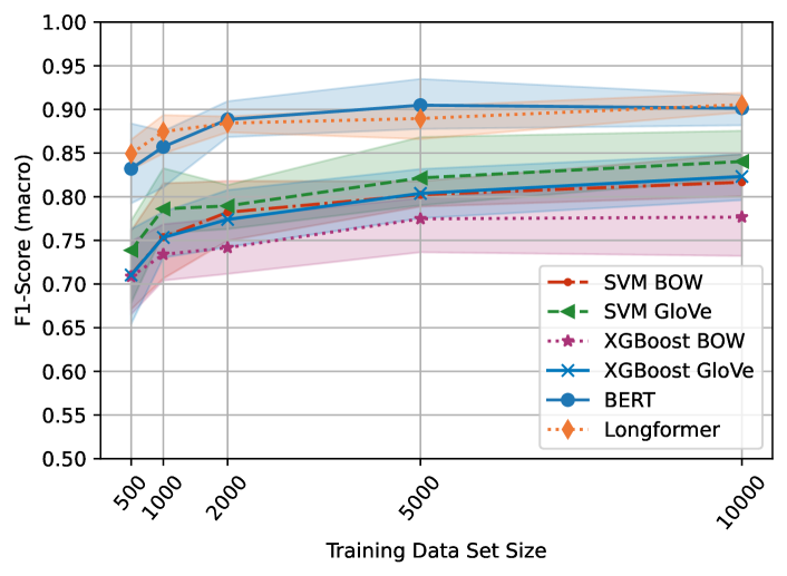
Figure 10: Performances on Toxic Application with Varying Training Data Set Sizes. For each training data set size and each model, the plotted symbols indicate the mean of the test set macro-averaged $F_{1}$-Scores across the five iterations. The shaded areas range from the minimum to the maximum macro-averaged $F_{1}$-Score obtained across the five iterations.

Across all evaluated classification tasks and training data set sizes, the Transformer-based models for transfer learning tend to achieve higher macro-averaged $F_{1}$-Scores than the conventional machine learning algorithms SVM and XGBoost. As has been observed before, the classic machine learning algorithms produce acceptable results given the relatively simple representations of text they are applied on. However, when compared on the basis of the (mean) macro-averaged $F_{1}$-Scores presented in Table 1, BERT, RoBERTa, and the Longformer consistently outperform the best performing conventional model by a margin of at minimum $0.05$ to $0.11$. These moderate to considerably higher prediction performances across all evaluated textual styles, sequence lengths, and especially the smaller training data set sizes, demonstrate the potential benefits that neural transfer learning with Transformers can bring to analyses in which a researcher aims at having a valid text-based measure of a concept and thus seeks to replicate human codings as accurately as possible. Even if only a small to medium-sized training data set is available, social scientists that apply Transformer-based models in a transfer learning setting are likely to obtain more valid measures for concepts that they measure from texts. A detailed examination of the macro-averaged $F_{1}$-Scores reveals further findings:

• Averaged GloVe representations partly, though not consistently, produce a slight advantage over basic BOW preprocessing. This emphasizes that employing transfer learning on conventional machine learning algorithms by extracting pretrained features (here: GloVe embeddings) and taking them as the data representation input might be beneficial—even if averaging over the embeddings erases information on word order and dependencies.

• For the Ethos and Abortion applications, RoBERTa outperforms BERT to a small extent. This finding is consistent with previous research (Liu et al., 2019, p. 7). In general, it is difficult to disentangle the effects of single modifications of the original BERT architecture and pretraining settings that BERT-extensions as RoBERTa implement (Aßenmacher & Heumann, 2020). It is likely, however, that one important contribution is the longer pretraining on more and more varied data. Whereas BERT is pretrained on a corpus of books and Wikipedia articles, RoBERTa is additionally pretrained on three more large data sets that are based on text passages from the web (Liu et al., 2019, p. 5-6). The larger and more heterogeneous pretraining corpus is likely to enable RoBERTa to produce representations that better generalize across a diverse set of target task corpora as inspected here.

• In the Ethos application, BERT and RoBERTa do not only exceed the performances of the other evaluated models but also the best performing model developed by Duthie & Budzynska, (2018). To differentiate non-ethotic from positive and from negative ethotic sentences, Duthie & Budzynska, (2018) had created an elaborate NLP pipeline including a POS tagger, dependency parsing, anaphora resolution, entity extraction, sentiment classification, and a deep RNN. Duthie & Budzynska, (2018, p. 4045) report a macro-averaged $F_{1}$-Score of $0.65$ for their best model. BERT and RoBERTa here surpass this performance. As the pretrained BERT and ROBERTa models are simply fine-tuned to the Ethos classification target task without implementing (and having to come up with) an extensive and complex preprocessing pipeline, this demonstrates the efficiency and power of transfer learning.

• With all models achieving only mediocre performances, the Abortion classification task, for which only $653$ short Tweets are available as training instances, seems to be especially difficult. BERT and RoBERTa still surpass SVM and XGBoost but with a slightly smaller margin. By applying an SVM with a linear kernel based on word and character n-gram feature representations, Mohammad et al., (2017, p. 13) reach classification performance levels that are higher than the ones reached by the models presented here. The Abortion classification task with short tweets in which the mere $N$-grams tend to be indicative of the stance toward the issue (Mohammad et al., 2017, p. 13), seems to be an example of a task in which deep learning models only produce a moderate advantage or—if it is easy to select BOW representations that very well capture linguistic variation that helps in discriminating the texts into the categories—even no advantage over traditional machine learning algorithms.

• Across all evaluated training data set sizes, the Transformer-based models with transfer learning tend to be better at solving the Toxic comment classification task compared to the conventional algorithms (see Figure 10). As is to be expected, the performance levels for all models decrease with decreasing training data set sizes. Yet although the neural models have much more parameters to learn, their macro-averaged $F_{1}$-Scores do not decrease more sharply than those of the traditional machine learning algorithms. Especially as training data sets become small, the effectiveness of representations from pretrained models becomes salient. Here, the pretrained models seem to function as a quite effective input to the target task.

• Whereas the Longformer processes text sequences of 1,024 tokens, the input sequences for BERT were truncated at 512 tokens for the Toxic application. Despite this large difference in sequence lengths, BERT only slightly underperforms compared to the Longformer—and matches the Longformer for larger training data set sizes. As only a small share of comments in the Wikipedia Toxic Comment Dataset are longer than 512 tokens (see again Figure 9h), the Longformer’s advantage of being able to process longer text sequences does not materialize here. Removing tokens from the middle of comments that exceed 512 tokens does not harm BERT’s prediction performance and is an effective workaround in this application. For applications based on corpora in which the mass of the sequence length distribution is above 512 tokens, however, the Longformer’s ability to process and capture the information contained in these longer documents, is likely to be important for prediction performance.

• The time consumed during training differs substantively between the conventional and the Transformer models. Larger training data sets and smaller batch sizes increase the time required for fine-tuning the pretrained Transformer models. Across the applications presented here, the absolute training time varies between 1 and 276 seconds for SVM BOW, between 32 and 2,272 seconds for BERT and 31 to 9,707 seconds for RoBERTa/Longformer.

• An additional analysis that explores the effectiveness of zero-shot learning is conducted (see Appendix J). Across all applications, across both employed pretrained models (RoBERTa and BART), and across all explored hypothesis formulations, the macro-averaged $F_{1}$-Scores are mediocre and substantially lower than for the fine-tuned models. The highest macro averaged $F_{1}$-Scores from zero-shot learning are 0.200 (Ethos), 0.455 (Abortion), and 0.470 (Toxic). Even if the prediction performances of the here implemented zero-shot learning framework are not sufficiently high in order to be applied in research projects in which researchers seek to as accurately as possible measure a priori-defined concepts from texts, this analysis nevertheless demonstrates what can be achieved with representations from pretrained models alone.

7 Discussion

Advances in NLP research on transfer learning and the attention mechanism, that is incorporated in the Transformer, have paved the way to a new mode of learning in which researchers can hope to achieve higher prediction performances by taking a readily available pretrained model and fine-tuning it, with a manageable amount of resources, to their NLP task of interest (Bommasani et al., 2021). These advances are of interest to social scientists that attempt to have valid measures of concepts from text data but may have limited amounts of training data and resources. To use the potential advantages for social science text analysis, this study has presented and applied Transformer-based models for transfer learning. In the supervised classification tasks evaluated in this study, transfer learning with Transformer models outperformed traditional machine learning across all tasks and data set sizes.

Employing transfer learning with Transformer-based models, however, will not always perform better compared to other machine learning algorithms and is not the most adequate strategy for each and every text-based research question. As the attention mechanism is specialized in capturing dependencies and contextual meanings, these models are likely to generate more accurate predictions if contextual information and long-range dependencies between tokens are relevant for the task at hand. They are less likely to provide much of an advantage if the function to be learned between textual inputs and desired outputs is less complex—for example because single $N$-grams are strongly indicative of class labels (see e.g. the Abortion application).

Transformer-based models for transfer learning furthermore are useful for supervised classification tasks in which the aim is to achieve an as high as possible prediction performance rather than having an interpretable model. Social scientists whose primary goal is to have as precise as possible text-based measures for concepts they employ may find Transformer-based models for transfer learning highly useful, whereas researchers whose primary goal is to know which textual features are most important in discriminating between class labeled documents (e.g. Slapin & Kirkland, 2020) are likely to be better served with directly interpretable models.

Moreover, due to the sequence length limitations of Transformer-based models, the applicability of these models is currently restricted to NLP tasks that operate on only moderately long text sequences. Research that seeks to reduce the memory resources consumed by the attention mechanism and thus allows for processing longer text sequences is highly important because it opens up the potential of Transformers for a wider range of social science text analyses.

As neural transfer learning with Transformers is the basis of larger developments within AI research (Bommasani et al., 2021), it is important that social scientists understand these new learning modes and models—such that these learning modes and models can be correctly and fruitfully applied and their risks critically assessed.

Appendix

Appendix A Introduction to Deep Learning

This section provides an introduction to the basics of deep learning. First, based on the example of feedforward neural networks the core elements of neural network architectures are explicated. Then, the optimization process via stochastic gradient descent with backpropagation (Rumelhart et al., 1986) will be presented. Subsequently, the architecture of recurrent neural networks (RNNs) (Elman, 1990) is outlined.

A.1 Feedforward Neural Network

The most elementary deep learning model is a feedforward neural network (Goodfellow et al., 2016, p. 164). A feedforward neural network with $L$ hidden layers, vector input $\bm{x}$, and a scalar output $y$ can be visualized as in Figure 11 and be described as follows:

$$\bm{h}_{1}=\sigma_{1}(\bm{W}_{1}\bm{x}+\bm{b}_{1})$$ (17)

$$\bm{h}_{2}=\sigma_{2}(\bm{W}_{2}\bm{h}_{1}+\bm{b}_{2})$$ (18)

$$\dots$$

$$\bm{h}_{l}=\sigma_{l}(\bm{W}_{l}\bm{h}_{l-1}+\bm{b}_{l})$$ (19)

$$\dots$$

$$y=\sigma_{o}(\bm{w}_{o}\bm{h}_{L}+b_{o})$$ (20)

The input to the neural network is the $K_{0}$-dimensional vector $\bm{x}$ (see Equation 17). $\bm{x}$ enters an affine function characterized by weight matrix $\bm{W}_{1}$ and bias vector $\bm{b}_{1}$, where $\bm{W}_{1}\in\mathbb{R}^{K_{1}\times K_{0}}$, and $\bm{b}_{1}\in\mathbb{R}^{K_{1}}$. $\sigma_{1}$ is a nonlinear activation function and $\bm{h}_{1}\in\mathbb{R}^{K_{1}}$ is the $K_{1}$-dimensional representation of the data in the first hidden layer. This is, the neural networks takes the input data $\bm{x}$ and via combining an affine function with a nonlinear activation function generates a new, transformed representation of the original input: $\bm{h}_{1}$. The hidden state $\bm{h}_{1}$ in turn serves as the input for the next layer that produces representation $\bm{h}_{2}\in\mathbb{R}^{K_{2}}$. This continues through the layers until the last hidden representation, $\bm{h}_{L}\in\mathbb{R}^{K_{L}}$, enters the output layer (see Equation 20).

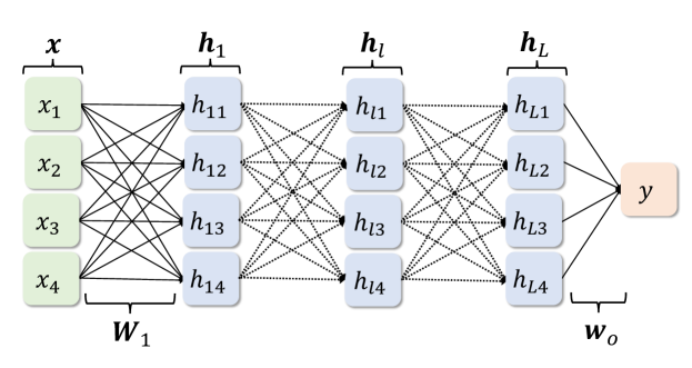
Figure 11: A Feedforward Neural Network. Feedforward neural network with $L$ hidden layers, four units per hidden layer and scalar output $y$. The solid lines indicate the linear transformations of weight matrix $\bm{W}_{1}$. The dotted lines indicate the connections between several consecutive hidden layers.

The activation functions in neural networks are typically chosen to be nonlinear (Goodfellow et al., 2016, p. 168). The reason is that if the activation functions were set to be linear, the output of the neural network would merely be a linear function of $\bm{x}$ (Goodfellow et al., 2016, p. 168). Hence, the use of nonlinear activation functions is essential for the capacity of neural networks to approximate a wide range of functions and highly complex functions (Ruder, 2019a , p. 31).

In the hidden layers, the Rectified Linear Unit (ReLU) (Nair & Hinton, 2010) is often used as an activation function $\sigma_{l}$ (Goodfellow et al., 2016, p. 171). If $\bm{q}=[q_{1},\dots,q_{k},\dots,q_{K}]$ is the $K$-dimensional vector resulting from the affine transformation in the $l$th hidden layer, $\bm{q}=\bm{W}_{l}\bm{h}_{l-1}+\bm{b}_{l}$ (see Equation 19), then ReLU is applied on each element $q_{k}$:

$$\sigma_{l}(\bm{q})_{k}=max\{0,q_{k}\}$$ (21)

$\sigma_{l}(\bm{q})_{k}$ then is the $k$th element of hidden state vector $\bm{h}_{l}$.

In the output layer, the activation function $\sigma_{o}$ is selected so as to produce an output that matches the task-specific type of output values. In binary classification tasks with $y_{i}\in\{0,1\}$ the standard logistic function, often simply referred to as the sigmoid function, is a common choice (Goodfellow et al., 2016, p. 179-180). For a single observational unit $i$, the sigmoid function’s scalar output value gives the probability that $y_{i}=1$. If $y_{i}$, however, can assume one out of $C$ unordered response category values, $y_{i}\in\{\mathcal{G}_{1},\dots,\mathcal{G}_{c},\dots,\mathcal{G}_{C}\}$, then the softmax function (which is a generalization of the sigmoid function that takes as an input and produces as an output a vector of length $C$) is typically employed (Goodfellow et al., 2016, p. 180-181). For the $i$th example, the $c$th element of the softmax output vector gives the predicted probability that unit $i$ falls into the $c$th class.

A.2 Optimization: Gradient Descent with Backpropagation

In supervised learning tasks, a neural network is provided with input $\bm{x}_{i}$ and corresponding output $y_{i}$ for each training example. All the weights and bias terms are parameters to be learned in the process of optimization (Goodfellow et al., 2016, p. 165). The set of parameters hence is $\bm{\theta}=\{\bm{W}_{1},\dots,\bm{W}_{l},\dots,\bm{W}_{L},\bm{W}_{o},\bm{b}_{1},\dots,\bm{b}_{l},\dots,\bm{b}_{L},\bm{b}_{o}\}$.

For a single training example $i$, the loss function $\mathcal{L}(y_{i},\mathsf{f}(\bm{x}_{i},\bm{\tilde{\theta}}))$ measures the discrepancy between the value predicted for unit $i$ by model $\mathsf{f}(\bm{x}_{i},\bm{\tilde{\theta}})$, that is characterized by the estimated parameter set $\bm{\tilde{\theta}}$, and the true value $y_{i}$ (Vapnik, 1991, p. 832). In the optimization process, the aim is to find the set of values for the weights and biases that minimizes the average of the observed losses over all training set instances, also known as the empirical risk: $\mathcal{R}_{emp}(\bm{\tilde{\theta}})=\frac{1}{N}\sum_{i=1}^{N}\mathcal{L}(y_{i},\mathsf{f}(\bm{x}_{i},\bm{\tilde{\theta}}))$ (Goodfellow et al., 2016, p. 272-273).

Neural networks commonly employ variants of gradient descent with backpropagation in the optimization process (Goodfellow et al., 2016, p. 173). To approach the local minimum of the empirical risk function, the gradient descent algorithm makes use of the fact that the direction of the negative gradient of function $\mathcal{R}_{emp}$ at current point $\bm{\tilde{\theta}_{j}}$ gives the direction in which $\mathcal{R}_{emp}$ is decreasing fastest—the direction of the steepest descent (Goodfellow et al., 2016, p. 83). The gradient is a vector of partial derivatives. It is the derivative of $\mathcal{R}_{emp}$ at point $\bm{\tilde{\theta}_{j}}$ and is denoted as $\nabla_{\bm{\tilde{\theta}_{j}}}\mathcal{R}_{emp}(\bm{\tilde{\theta}_{j}})$ (Johnson, 2017, p. 2).

In the $j$th iteration, the gradient descent algorithm computes the negative gradient of $\mathcal{R}_{emp}$ at current point $\bm{\tilde{\theta}_{j}}$ and then changes its position from $\bm{\tilde{\theta}_{j}}$ into the direction of the negative gradient (Goodfellow et al., 2016, p. 83-84):

$$\bm{\tilde{\theta}_{j+1}}=\bm{\tilde{\theta}_{j}}-\eta\nabla_{\bm{\tilde{\theta}_{j}}}\mathcal{R}_{emp}(\bm{\tilde{\theta}_{j}})$$ (22)

where $\eta\in\mathbb{R}_{+}$ is the learning rate. If $\eta$ is small enough, then $\mathcal{R}_{emp}(\bm{\tilde{\theta}_{j}})\geq\mathcal{R}_{emp}(\bm{\tilde{\theta}_{j+1}})\geq\mathcal{R}_{emp}(\bm{\tilde{\theta}_{j+2}})\geq\dots$. This is, repeatedly updating into the direction of the negative gradient with a suitably small learning rate $\eta$, will generate a sequence moving toward the local minimum (Li et al., 2020a ).

In each iteration, the gradients for all parameters are computed via the backpropagation algorithm (Rumelhart et al., 1986). A very frequently employed approach, known as mini-batch stochastic gradient descent, is to compute the gradients based on a random sample, a mini-batch, of $S$ training set observations (Goodfellow et al., 2016, p. 275-276, 291):

$$\nabla_{\bm{\tilde{\theta}_{j}}}\mathcal{R}_{emp}(\bm{\tilde{\theta}_{j}})=\frac{1}{S}\sum_{s=1}^{S}\nabla_{\bm{\tilde{\theta}_{j}}}\mathcal{L}(y_{s},\mathsf{f}(\bm{x}_{s},\bm{\tilde{\theta}_{j}}))$$ (23)

The learning rate $\eta$ and the size of the mini-batch $S$ are hyperparameters in training neural networks. Especially the learning rate is often attended to carefully (Li et al., 2020a ). A too high learning rate leads to large fluctuations in the loss function values, whereas a too low learning rate implies slow convergence and risks that the learning process does not move away from a non-optimal region with a high loss value (Goodfellow et al., 2016, p. 291). Commonly, the learning rate is set to vary over the course of the training process (Goodfellow et al., 2016, p. 290-291). Furthermore, there are variants of stochastic gradient descent, e.g. AdaGrad (Duchi et al., 2011), RMSProp (Hinton et al., 2012), and Adam (Kingma & Ba, 2015), that have a different learning rate for each parameter (Goodfellow et al., 2016, p. 303-305).

A.3 Recurrent Neural Networks

The recurrent neural network (RNN) (Elman, 1990) is the most basic neural network to process sequential input data of variable length such as texts (Goodfellow et al., 2016, p. 367). Given an input sequence of $T$ input embeddings $(\bm{z}_{[a_{1}]},\dots,\bm{z}_{[a_{t}]},\dots,\bm{z}_{[a_{T}]})$, RNNs sequentially process each token. Here, one input embedding $\bm{z}_{[a_{t}]}$ corresponds to one time step $t$ and the hidden state $\bm{h}_{t}$ is updated at each time step. At each step $t$, the hidden state $\bm{h}_{t}$ is a function of the hidden state generated in the previous time step, $\bm{h}_{t-1}$, and new input data, $\bm{z}_{[a_{t}]}$ (see Figure 12) (Elman, 1990; Amidi & Amidi, 2019).

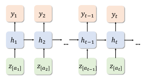
Figure 12: A Recurrent Neural Network. Architecture of a basic RNN unfolded through time. At time step $t$, the hidden state $\bm{h}_{t}$ is a function of the previous hidden state, $\bm{h}_{t-1}$, and current input embedding $\bm{z}_{[a_{t}]}$. $\bm{y}_{t}$ is the output produced at $t$.

The hidden states $\bm{h}_{t}$, that are passed on and transformed through time, serve as the model’s memory (Elman, 1990, p. 182; Ruder, 2019a , p. 32). They capture the information of the sequence that entered until $t$ (Goldberg, 2016, p. 391). Due to this sequential architecture, RNNs theoretically can model dependencies over the entire range of an input sequence (Amidi & Amidi, 2019). But in practice, recurrent models have problems learning dependencies that extend beyond sequences of 10 or 20 tokens (Goodfellow et al., 2016, p. 396-399). The reason is that when backpropagating the gradients through the time steps (Backpropagation Through Time (BPTT)), the gradients may vanish and thus fail to transmit a signal over long ranges (Goodfellow et al., 2016, p. 396-399).

The long short-term memory (LSTM) model (Hochreiter & Schmidhuber, 1997) extends the RNN with input, output, and forget gates that enable the model to accumulate, remember, and forget provided information (Goldberg, 2016, p. 399-400). This makes LSTMs better suited than the basic RNNs to model dependencies stretching over long time spans (Goldberg, 2016, p. 399-400).

Appendix B Zero-Shot Learning and the GPT-3

Ultimately the aim of the strand of NLP research focusing on zero-shot learning is to have a model that generalizes well to a wide spectrum of target tasks without being explicitly trained on the target tasks (Radford et al., 2019; Brown et al., 2020; Davison, 2020b ). The work on the series of GPT models—OpenAI GPT (Radford et al., 2018), GPT-2 (Radford et al., 2019), and especially GPT-3 (Brown et al., 2020)—has demonstrated that large models that are pretrained on language modeling tasks on excessively large corpora can sometimes come close to achieving acceptable prediction performances without fine-tuning (i.e. without gradient updates) on target task-specific examples (Brown et al., 2020, p. 4). So far, the key to increasing the zero-shot no-fine-tuning learning performances seems to be an increase in the models’ capacity to learn complex functions as determined by the number of model parameters (Brown et al., 2020, p. 4). (Whilst the original OpenAI GPT comprises $117$ million parameters, GPT-2 has $1,542$ million (Radford et al., 2019, p. 4) and GPT-3 has 175,000 million parameters (Brown et al., 2020, p. 1, 8).) Additionally, and in correspondence with an increase in model parameters, the size of the employed training corpora increases rapidly as well (Radford et al., 2019, p. 3; Brown et al., 2020, p. 5). Yet given its sheer size, re-training the GPT-3 is prohibitively expensive (Brown et al., 2020, p. 9; Riedl, 2020). Moreover, whereas typically the source code of pretrained language models is open sourced by the companies (e.g. Google, Facebook, Microsoft) that developed these models, OpenAI decided not to share the code on GPT-3 and instead allows using GPT-3 for downstream tasks via an API, thereby raising questions regarding accessibility and replicability of pretrained language models for research (Brockman et al., 2020; Riedl, 2020).

Appendix C Subword Tokenization Algorithms

Subword tokenization algorithms try to find a balance between word-level tokenization (which tends to result in a large vocabulary—and hence a large embedding matrix that consumes a lot of memory) and character-level tokenization (which generates a small and flexible vocabulary but does not yield as well-performing representations of text) (Radford et al., 2019, p. 4; Hugging Face, 2020c ). Subword tokenization algorithms typically result in vocabularies in which frequently occurring character sequences are merged to form words whereas less common character sequences become subwords or remain separated as single characters (Radford et al., 2019, p. 4; Hugging Face, 2020c ). The Byte-Pair Encoding (BPE) algorithm and variants thereof are subword tokenization algorithms employed in many Transformer-based models (e.g. Devlin et al., 2019; Liu et al., 2019; Radford et al., 2019). The base BPE algorithm starts with a list of all the unique characters in a corpus and then learns to merge the characters into longer character sequences (eventually forming subwords and words) until the desired vocabulary size is reached (Sennrich et al., 2016, p. 1717-1718). In the WordPiece variant of BPE, the algorithm merges at each step the character pair that, when merged, results in the highest increase in the likelihood of the training corpus compared to all other pairs (Schuster & Nakajima, 2012, p. 5150).

Appendix D Pretraining BERT

In the masked language modeling pretraining task, for each token $q$, that has been sampled for prediction, the updated token representation produced by the last encoder $\bm{h}^{*}_{q}$ is fed into a single-layer feedforward neural network with a softmax output layer to generate a probability distribution over the terms in the vocabulary predicting the term corresponding to $q$ (see Figure 7 in the main article) (Alammar, 2018a, ; Devlin et al.,, 2019, p. 4174). For the next sentence prediction task, the representation for the [CLS] token, $\bm{h}^{*}_{1}$, is processed via a single-layer feedforward neural network with a softmax output to give the predicted probability of the second segment succeeding the first segment (see Figure 7 in the main article) (Alammar, 2018a, ; Devlin et al.,, 2019, p. 4174). The loss function in pretraining is the sum of the average loss from the masked language modeling task and the average loss from next sentence prediction (Devlin et al., 2019, p. 4183).

In order to learn the parameters in pretraining, the authors use the Adam algorithm, a variant of stochastic gradient descent, in which at the $j$th iteration for each individual parameter the estimate of the gradient’s average for this parameter is updated based on a parameter-specific learning rate (Kingma & Ba,, 2015; Devlin et al.,, 2019, p. 4183). They use a learning rate schedule in which the global Adam learning rate (that is individually adapted per parameter) linearly increases during the first 10,000 iterations (the warmup) to reach a maximum value of 1e-4 and then is linearly decaying (Devlin et al., 2019, p. 4183). They furthermore regularize by employing an $L^{2}$ weight decay (Goodfellow et al., 2016, p. 226; Devlin et al., 2019, p. 4183). As an additional regularization strategy they use dropout (Srivastava et al., 2014) with dropout probability $p=0.1$ (Devlin et al., 2019, p. 4183). In dropout, units and their corresponding connections are randomly dropped during training (Srivastava et al., 2014, p. 1929). Devlin et al., (2019, p. 4183) select a mini-batch size of 256 sequences and conduct 1,000,000 iterations, which implies that they train the model for around $40$ epochs; i.e. they make around $40$ passes over the entire $3.3$ billion token pretraining data set.

Appendix E Additional Examples for Autoencoding Models: ALBERT and ELECTRA

ALBERT (Lan et al., 2020) aims at a parameter efficient design. By decoupling the size of the input embedding layers from the size of the hidden layers and by sharing parameters across all layers, ALBERT substantially reduces the number of parameters to be learned (e.g. by a factor of 18 comparing ALBERT-Large to BERT_LARGE) (Lan et al., 2020, p. 2, 4, 6). Parameter reduction has regularizing effects, and—because it saves computational resources—allows to construct a deeper model with more and/or larger hidden layers whose increased capacity benefits performance on target tasks while still comprising fewer parameters than the original BERT_LARGE (Lan et al., 2020, p. 2, 7).

Whereas BERT, RoBERTa, and ALBERT make use of the masked language modeling task, ELECTRA introduces a new, more resource-efficient pretraining objective, named replaced token detection (Clark et al., 2020, p. 1). ELECTRA addresses the issue that in masked language modeling for each input sequence predictions are made only for those $15\%$ of tokens that have been sampled for the task, thereby reducing the amount of what could be learned from each training sequence (Clark & Luong, 2020). In pretraining, ELECTRA has to predict for each input token in each sequence whether the token comes from the original sequence or has been replaced by a plausible fake token (Clark & Luong, 2020; Clark et al., 2020, p. 1, 3). Thus, ELECTRA (the discriminator) solves a binary classification task for each token and is much more efficient in pretraining requiring fewer computational resources (Clark & Luong, 2020; Clark et al., 2020, p. 3). The plausible fake tokens come from a generator that is trained on a masked language modeling task together with the ELECTRA discriminator (Clark et al., 2020, p. 3). After pretraining, the generator is removed and only the ELECTRA discriminator is used for fine-tuning (Clark & Luong, 2020).

Appendix F Additional Example for an Autoregressive Model: The XLNet

Strictly speaking, XLNet (Yang et al., 2019) is not an autoregressive model (Hugging Face, 2020b ). Yet the permutation language modeling objective that it introduces builds on the autoregressive language modeling framework (Yang et al., 2019, p. 5756). The authors of XLNet seek a pretraining objective that learns bidirectional representations as in autoencoding models whilst overcoming problems of autoencoding representations: first, the pretrain-finetune discrepancy that results from the fact that ‘[MASK]’ tokens only occur in pretraining, and, second, the assumption that the tokens selected for the masked language modeling task in one sequence are independent of each other (Yang et al., 2019, p. 5754-5755). Given a sequence whose tokens are indexed $(1,\dots,T)$, the permutation language modeling objective makes use of the permutations of the token index $(1,\dots,T)$ (Yang et al., 2019, p. 5756). For each possible permutation of $(1,\dots,T)$, the task is to predict the next token in the permutation order given the previous tokens in the permutation (Yang et al., 2019, p. 5756). In doing so, the learned token representations can access information from left and right contexts whilst the autoregressive nature of the modeling objective avoids the pretrain-finetune discrepancy and the independence assumption (Yang et al., 2019, p. 5756).

Appendix G Examples for Sequence-to-Sequence Models: The T5 and BART

The T5 (Raffel et al., 2020) is very close to the original Transformer encoder-decoder architecture. It is based on the idea to consider all NLP tasks as text-to-text problems (Raffel et al., 2020, p. 2-3). To achieve this, each input sequence that is fed to the model is preceded by a task-specific prefix, that instructs the model what to do. For example (Raffel et al., 2020, p. 47ff.): A translation task in this scheme has the input ‘translate from English to German: I love this movie.’ and the model is trained to output ‘Ich liebe diesen Film.’. For a sentiment classification task on the SST-2 Dataset (Socher et al., 2013), the input would be: ‘sst2 sentence: I love this movie.’ and the model is trained to predict one of ‘positive’ or ‘negative’. The fact that there is a shared scheme for all NLP tasks, allows the T5 to be pretrained on a multitude of different NLP tasks before being fine-tuned on a specific target task (Raffel et al., 2020, p. 30-33). In the multitask pretraining mode, T5 is trained on a self-supervised objective similar to the masked language modeling task in BERT as well as various different supervised tasks (such as translation or natural language inference) (Raffel et al., 2020, p. 37). With this multitask pretraining setting, in which the parameters learned in pretraining are shared across different tasks, the T5, rather than being a standard sequential transfer learning model, implements a softened version of multitask learning (Raffel et al., 2020, p. 30).

BART (Lewis et al., 2020)—another well-known sequence-to-sequence model—is composed of an encoder and a decoder. Just as an autoencoding model, BART in pretraining is presented with a corrupted sequence and has to predict the original uncorrupted sequence (Lewis et al., 2020, p. 2). In pretraining, BART allows a wide range of different types of corrupting operations to be applied to the documents (Lewis et al., 2020, p. 2-3). Due to this autoencoding-style pretraining task, BART can be considered a BERT-like bidirectional encoder followed by an autoregressive unidirectional decoder (Lewis et al., 2020, p. 1-2). Because of the decoder, that learns to predict output tokens in an autoregressive manner, BART is better suited to perform text generation tasks than regular autoencoding models (Lewis et al., 2020, p. 1, 6). Additionally, BART performs similarly to RoBERTa on discriminative natural language understanding tasks (Lewis et al., 2020, p. 1, 6).

Appendix H Interpretability

One common method to make neural networks more interpretable is probing (also known as auxiliary prediction tasks) (Belinkov & Glass, 2019, p. 51). In probing, an element of a trained neural network (e.g. a set of contextualized token embeddings) is extracted, fixed, and fed into a simple classifier and then is applied to some task (e.g. POS tagging, coreference resolution) (Belinkov & Glass, 2019, p. 51; Tenney et al., 2019b , p. 1-3). If the prediction performance on the task is high, then this is taken as an indication that information required to address the task (e.g. syntactic information for POS tagging, semantic information for coreference resolution) is encoded in the tested element of the network (Belinkov & Glass, 2019, p. 51; Tenney et al., 2019b , p. 2). Accordingly, probing is one way to inspect what information a neural network has learned and which elements capture which information.

Another important aspect of interpretability is to assess the importance of input features for predicted outputs. The open-source library Captum (https://captum.ai/) implements several attribution algorithms that allow just that (Kokhlikyan et al., 2020, p. 3). Additionally, algorithms for attributing outputs to a hidden layer, as well as algorithms for attributing hidden layer values to feature inputs, are also provided (Kokhlikyan et al., 2020, p. 3).

Most attribution algorithms can be considered as either being gradient-based or perturbation-based (Agarwal et al., 2021, p. 110). Perturbation-based algorithms make use of removed or altered input features to learn about the importance of input features (Ancona et al., 2018, p. 2; Agarwal et al., 2021, p. 110). Gradient-based algorithms make use of the gradient of the predicted output with regard to input features (Ancona et al., 2018, p. 2-3; Agarwal et al., 2021, p. 110).

For models that incorporate attention mechanisms, the analysis of patterns in attention weights $\alpha_{t,t^{*}}$ and the probing of attention heads is another interpretability-related research area (see e.g. Clark et al., 2019; Kobayashi et al., 2020). Tools for interpreting attention matrices are also provided by Captum (see, for example, the tutorial at https://captum.ai/tutorials/Bert_SQUAD_Interpret2).

Another set of methods related to interpretability is behavioral testing and the construction of adversarial examples (Belinkov & Glass, 2019, p. 54-58). Here, the goal is to inspect a trained model’s behavior when confronted with a challenging set of inputs or adversarial examples. In an award-winning paper, Ribeiro et al., (2020) present a methodology for behavioral testing. Their research findings emphasize that whilst the performance of NLP models as evaluated via accuracy measures on held-out test sets has risen substantially during the last years (see also e.g. Wang et al., 2019, p. 2), when evaluating the models via behavioral testing, it is revealed that accuracy-based performances on common benchmark data sets overestimate the models’ linguistic and language understanding capabilities. BERT, for example, is found to have high failure rates for simple negation tests (e.g. classifying $84.4\%$ of positive or neutral tweets in which a negative sentiment expression is negated into the negative category) (Ribeiro et al., 2020, p. 4905-4907).

Appendix I Deep Learning and Transfer Learning in Practice

To practically implement deep learning models, it is advisable to have access to a graphics processing unit (GPU). In contrast to a central processing unit (CPU), a GPU comprises many more cores and can conduct thousands of operations in parallel (Caulfield, 2009). GPUs thus handle tasks that can be broken down into smaller, simultaneously executable subtasks much more efficiently than CPUs (Caulfield, 2009). When training a neural network via stochastic gradient descent, every single hidden unit within a layer usually can be updated independently of the other hidden units in the same layer (Goodfellow et al., 2016, p. 440). Hence, neural networks lend themselves to parallel processing.

A major route to access and use GPUs is via NVIDIA’s CUDA framework (Goodfellow et al., 2016, p. 440-441). But instead of additionally learning how to write CUDA code, researchers use libraries that enable CUDA GPU processing (Goodfellow et al., 2016, p. 441). As of today, PyTorch (Paszke et al., 2019) and TensorFlow (Abadi et al., 2016) are the most commonly used libraries that allow training neural networks via CUDA-enabled GPUs. Both libraries have Python interfaces. Therefore, to efficiently train deep learning models via GPU acceleration, researchers can use a programming language they are familiar with.

Another obstacle is having a GPU at hand that can be used for computation. The computing infrastructures of universities and research institutes typically provide their members access to GPU facilities. Free GPU usage also is available via Google Colaboratory (or Colab for short): https://colab.research.google.com/notebooks/intro.ipynb. Colab is a computing service that allows its user to run Python code via the browser (Google Colaboratory, 2020). Here, GPUs can be used free of cost. The free resources, however, are not guaranteed and there may be usage limits. One issue researchers have to keep in mind when using Colab is that at each session another type of GPU may be assigned. Documenting the used computing environment hence is vital to ensure traceability. Note, that full reproducibility across different computing platforms and across different versions of PyTorch and TensorFlow cannot be guaranteed (Freidank, 2020; Torch Contributors, 2021). However, there are measures that researchers can undertake to minimize nondeterministic elements (e.g. not using nondeterministic algorithms where possible and ensuring that batch allocation is reproducible) (see Torch Contributors, 2021).

Appendix J Application: Zero-Shot Learning

To explore how pretrained Transformer-based models would perform in a zero-shot learning setting, the approach of Yin et al., (2019) is followed. Yin et al., (2019, p. 3918-3919) frame zero-shot text classification as a natural language inference (NLI) task. In NLI, a model is presented with a premise and a hypothesis and then has to decide whether the hypothesis is true given the premise (entailment), whether the hypothesis is false given the premise (contradiction), or whether the hypothesis is neither true nor false given the premise (neutral) (see Table 2) (Williams et al., 2018, p. 1112-1113).

	[CLS]          … Premise …          [SEP]       … Hypothesis …         [SEP]	predict one out of
NLI	[CLS]   I am a lacto-vegetarian. [SEP]   I eat one egg per week.   [SEP]	entailment, contradict., neutral
ZSL	[CLS] Ok, I see what you mean. [SEP]   This comment is toxic.   [SEP]	entailment, contradict., neutral
2-3	[CLS] Ok, I see what you mean. [SEP] This comment is not toxic. [SEP]	entailment, contradict., neutral

Table 2: Scheme in Natural Language Inference (NLI) and Zero-Shot Learning (ZSL). In NLI, the model is provided with a premise followed by a hypothesis and has to decide whether the hypothesis is true (entailment), false (contradiction), or neutral (neutral) given the premise. In ZSL, the sequence for which a prediction is to be made constitutes the premise. Each class label is presented to the model as a separate hypothesis. Here, the input sequence is “Ok, I see what you mean.” and there are $C=2$ class labels, namely: $\{$toxic, not toxic$\}$. For each sequence-hypothesis pair the model has to predict one out of $\{$entailment, contradiction, neutral$\}$.

In the zero-shot classification framework of Yin et al., (2019), a model is presented with the input text (taking the role of the premise) and a hypothesis that asks whether the input text belongs to a particular class. The model then has to predict whether this is the case or not. The model that Yin et al., (2019) use for zero-shot learning is a BERT model that has been trained on three different NLI data sets (Yin et al., 2019, p. 3919). (The NLI data sets are, of course, unrelated to the target tasks Yin et al., (2019) use for zero-shot learning evaluation.)

Here, in a similar approach, two pretrained Transformer-based models—RoBERTa (Liu et al., 2019) and BART (Lewis et al., 2020)—that have been further trained on the Multi-Genre Natural Language Inference (MNLI) data set (Williams et al., 2018) are used as models for zero-shot learning. The models are accessed from Hugging Face’s Transformers and then are used in a zero-shot-classification pipeline that is based on an NLI-framework (see Davison, 2020a ). For an illustration see Table 2.

An important point to note is that the zero-shot performance will also depend on the textual formulation of the hypothesis the model is presented with (Yin et al., 2019, p. 3921-3922). (The model takes as an input the text sequence for which a prediction is to be made followed by the hypothesis and thus the model learns representations for the input sequence and the hypothesis and will generate a prediction based on (the compatibility) of both inputs (Davison, 2020b ).) Here, to explore the effect of different hypothesis formulations, two different hypothesis formulations are tried in each application (see Tables 3 and 4).

Moreover, note that if one has a target task with $C$ class labels such that $y_{i}\in\{\mathcal{G}_{1},\dots,\mathcal{G}_{c},\dots,\mathcal{G}_{C}\}$, then each class label is presented to the model as one separate hypothesis (Davison, 2020a ). Consequently, if there are, for example, $C=4$ labels, the model will be fed with $C=4$ different sequence-hypothesis pairs for each sequence. In the implementation in Hugging Face’s zero-shot-classification pipeline, the model generates for each of the $C$ sequence-hypothesis pairs a prediction to belong to one of $\{$entailment, contradiction, neutral$\}$ (Davison, 2020a ). Then, in order to aggregate the $C$ separate predictions into a single one, the predicted score for entailment is extracted for each hypothesis. Together, the $C$ entailment scores serve as the input to a softmax function that returns a $C$-dimensional vector of predicted probabilities (which sum to one) and the $c$th element gives the probability that the sequence belongs to the $c$th class (Davison, 2020a ).

The zero-shot classification results are presented in Tables 3 and 4. For each application, for each combination of an employed pretrained model and an explored hypothesis formulation, the macro-averaged $F_{1}$-Score for the test set is reported. Across applications, models, and hypothesis formulations, the achieved performance levels are mediocre compared to the macro-averaged $F_{1}$-Scores reached by the fine-tuned models (which are presented in Table 1 in the main article). Interestingly, the smallest reduction in performance compared to the fine-tuned models can be observed for the Abortion application. In contrast to the other two applications, that seek to measure concepts from text that are relatively difficult to adequately describe in words (ethos, toxicity), hypothesis formulation in the legalization of abortion application is relatively straightforward.

Source Code. Just as for the other analyses presented in this paper, the code for this zero-shot learning implementation is openly available in figshare at https://doi.org/10.6084/m9.figshare.14394173.

Ethos
Model Hypothesis Formulation Class Labels $F_{1}$ (macro) RoBERTa The statement {} the ethos of another politician or party. {attacks, does not refer to, 0.200 supports} RoBERTa The statement expresses {} sentiment toward the character of another politician or party. {negative, 0.188 no, positive} BART The statement {} the ethos of another politician or party. {attacks, 0.184 does not refer to, supports} BART The statement expresses {} sentiment toward the character of another politician or party. {negative, 0.181 no, positive}
Abortion
Model Hypothesis Formulation Class Labels $F_{1}$ (macro) RoBERTa The text is {} legalization of abortion. {in favor of, neutral toward, 0.344 against} RoBERTa The text expresses a {} stance toward legalization of abortion. {positive, neutral, 0.362 negative} BART The text is {} legalization of abortion. {in favor of, neutral toward, 0.455 against} BART The text expresses a {} stance toward legalization of abortion. {positive, neutral, 0.368 negative}

Table 3: ZSL Results I. Macro-averaged $F_{1}$-Scores obtained via zero-shot learning for the test sets of the Ethos and Abortion classification tasks. In each application, two pretrained models (RoBERTa and BART both trained on the MNLI) and two hypothesis formulations are explored. Gray colored numbers highlight the best performing model-hypothesis formulation combination for the task.

Toxic
Model Hypothesis Formul. Class Labels $F_{1}$ (macro) RoBERTa This comment is {}. {not toxic, toxic} 0.470 RoBERTa This comment is {}. {{neither obscene, nor threatening, nor insulting, and does not expresses hatred toward social groups and identities}, {obscene, or threatening, or insulting, or expresses hatred toward social groups and identities}} 0.213 BART This comment is {}. {not toxic, toxic} 0.378 BART This comment is {}. {{neither obscene, nor threatening, nor insulting, and does not expresses hatred toward social groups and identities}, {obscene, or threatening, or insulting, or expresses hatred toward social groups and identities}} 0.178

Table 4: ZSL Results II. Macro-averaged $F_{1}$-Scores obtained via zero-shot learning for one sampled test set ($N$ = 1,000) of the Toxic classification task. Two pretrained models (RoBERTa and BART both trained on the MNLI) and two hypothesis formulations are explored. Gray-colored numbers highlight the best performing model-hypothesis formulation combination for the task.

References

- Abadi et al., (2016) Abadi, M., Agarwal, A., Barham, P., Brevdo, E., Chen, Z., Citro, C., Corrado, G. S., Davis, A., Dean, J., Devin, M., Ghemawat, S., Goodfellow, I., Harp, A., Irving, G., Isard, M., Jia, Y., Jozefowicz, R., Kaiser, L., Kudlur, M., Levenberg, J., Mane, D., Monga, R., Moore, S., Murray, D., Olah, C., Schuster, M., Shlens, J., Steiner, B., Sutskever, I., Talwar, K., Tucker, P., Vanhoucke, V., Vasudevan, V., Viegas, F., Vinyals, O., Warden, P., Wattenberg, M., Wicke, M., Yu, Y., & Zheng, X. (2016). TensorFlow: Large-scale machine learning on heterogeneous distributed systems. arXiv. https://arxiv.org/abs/1603.04467
- Agarwal et al., (2021) Agarwal, S., Jabbari, S., Agarwal, C., Upadhyay, S., Wu, S., & Lakkaraju, H. (2021). Towards the unification and robustness of perturbation and gradient based explanations. Proceedings of Machine Learning Research, 139, 110–119. https://proceedings.mlr.press/v139/agarwal21c.html
- Akbik et al., (2018) Akbik, A., Blythe, D., & Vollgraf, R. (2018). Contextual string embeddings for sequence labeling. In E. M. Bender, L. Derczynski, & P. Isabelle (Eds.), Proceedings of the 27th International Conference on Computational Linguistics (pp. 1638–1649). Association for Computational Linguistics. https://aclanthology.org/C18-1139
- (4) Alammar, J. (2018a). The illustrated BERT, ELMo, and co. (How NLP cracked transfer learning). Jay Alammar. http://jalammar.github.io/illustrated-bert/
- (5) Alammar, J. (2018b). The illustrated Transformer. Jay Alammar. http://jalammar.github.io/illustrated-transformer/
- (6) Alammar, J. (2018c). Visualizing a neural machine translation model (mechanics of seq2seq models with attention). Jay Alammar. https://jalammar.github.io/visualizing-neural-machine-translation-mechanics-of-seq2seq-models-with-attention/
- Amidi & Amidi, (2019) Amidi, A. & Amidi, S. (2019). Recurrent neural networks cheatsheet [Lecture Notes]. Stanford University. https://stanford.edu/~shervine/teaching/cs-230/cheatsheet-recurrent-neural-networks
- Amsalem et al., (2020) Amsalem, E., Fogel-Dror, Y., Shenhav, S. R., & Sheafer, T. (2020). Fine-grained analysis of diversity levels in the news. Communication Methods and Measures, 14(4), 266–284. https://doi.org/10.1080/19312458.2020.1825659
- Anastasopoulos & Bertelli, (2020) Anastasopoulos, L. J. & Bertelli, A. M. (2020). Understanding delegation through machine learning: A method and application to the European Union. American Political Science Review, 114(1), 291–301. https://doi.org/10.1017/S0003055419000522
- Ancona et al., (2018) Ancona, M., Ceolini, E., Öztireli, C., & Gross, M. (2018). Towards better understanding of gradient-based attribution methods for deep neural networks. In Y. Bengio & Y. LeCun (Eds.), 6th International Conference on Learning Representations (ICLR 2018). https://openreview.net/pdf?id=Sy21R9JAW
- Aribandi et al., (2022) Aribandi, V., Tay, Y., Schuster, T., Rao, J., Zheng, H. S., Mehta, S. V., Zhuang, H., Tran, V. Q., Bahri, D., Ni, J., Gupta, J., Hui, K., Ruder, S., & Metzler, D. (2022). Ext5: Towards extreme multi-task scaling for transfer learning. In K. Hofmann & A. Rush (Eds.), International Conference on Learning Representations (ICLR 2022). https://openreview.net/forum?id=Vzh1BFUCiIX
- Aßenmacher & Heumann, (2020) Aßenmacher, M. & Heumann, C. (2020). On the comparability of pre-trained language models. In S. Ebling, D. Tuggener, M. Hürlimann, M. Cieliebak, & M. Volk (Eds.), Proceedings of the 5th Swiss Text Analytics Conference (SwissText) & 16th Conference on Natural Language Processing (KONVENS 2020). CEUR-WS.org. http://ceur-ws.org/Vol-2624/paper2.pdf
- Ba et al., (2016) Ba, J. L., Kiros, J. R., & Hinton, G. E. (2016). Layer Normalization. arXiv. https://arxiv.org/abs/1607.06450
- Babu et al., (2021) Babu, A., Wang, C., Tjandra, A., Lakhotia, K., Xu, Q., Goyal, N., Singh, K., von Platen, P., Saraf, Y., Pino, J., Baevski, A., Conneau, A., & Auli, M. (2021). XLS-R: Self-supervised cross-lingual speech representation learning at scale. arXiv. https://arxiv.org/abs/2111.09296
- Baevski et al., (2020) Baevski, A., Zhou, Y., Mohamed, A., & Auli, M. (2020). wav2vec 2.0: A framework for self-supervised learning of speech representations. In H. Larochelle, M. Ranzato, R. Hadsell, M. Balcan, & H. Lin (Eds.), Advances in Neural Information Processing Systems 33 (pp. 12449–12460). Curran Associates, Inc. https://proceedings.neurips.cc/paper/2020/file/92d1e1eb1cd6f9fba3227870bb6d7f07-Paper.pdf
- Bahdanau et al., (2015) Bahdanau, D., Cho, K., & Bengio, Y. (2015). Neural machine translation by jointly learning to align and translate. In Y. Bengio & Y. LeCun (Eds.), 3rd International Conference on Learning Representations (ICLR 2015). https://arxiv.org/abs/1409.0473
- Bapna et al., (2021) Bapna, A., Chung, Y.-a., Wu, N., Gulati, A., Jia, Y., Clark, J. H., Johnson, M., Riesa, J., Conneau, A., & Zhang, Y. (2021). SLAM: A unified encoder for speech and language modeling via speech-text joint pre-training. arXiv. https://arxiv.org/abs/2110.10329
- Barberá et al., (2021) Barberá, P., Boydstun, A. E., Linn, S., McMahon, R., & Nagler, J. (2021). Automated text classification of news articles: A practical guide. Political Analysis, 29(1), 19–42. https://doi.org/10.1017/pan.2020.8
- Belinkov & Glass, (2019) Belinkov, Y. & Glass, J. (2019). Analysis methods in neural language processing: A survey. Transactions of the Association for Computational Linguistics, 7, 49–72. https://doi.org/10.1162/tacl_a_00254
- Beltagy et al., (2020) Beltagy, I., Peters, M. E., & Cohan, A. (2020). Longformer: The long-document Transformer. arXiv. https://arxiv.org/abs/2004.05150
- Bengio et al., (2003) Bengio, Y., Ducharme, R., Vincent, P., & Janvin, C. (2003). A neural probabilistic language model. Journal of Machine Learning Research, 3, 1137–1155. https://www.jmlr.org/papers/v3/bengio03a.html
- Benoit, (2020) Benoit, K. (2020). Text as data: An overview. In L. Curini & R. Franzese (Eds.), The SAGE Handbook of Research Methods in Political Science and International Relations (pp. 461–497). SAGE Publications. https://www.doi.org/10.4135/9781526486387.n29
- Benoit et al., (2018) Benoit, K., Watanabe, K., Wang, H., Nulty, P., Obeng, A., Müller, S., & Matsuo, A. (2018). quanteda: An R package for the quantitative analysis of textual data. Journal of Open Source Software, 3(30), 774. https://doi.org/10.21105/joss.00774
- Bojanowski et al., (2017) Bojanowski, P., Grave, E., Joulin, A., & Mikolov, T. (2017). Enriching word vectors with subword information. Transactions of the Association for Computational Linguistics, 5, 135–146. https://doi.org/10.1162/tacl_a_00051
- Bommasani et al., (2021) Bommasani, R., Hudson, D. A., Adeli, E., Altman, R., Arora, S., von Arx, S., Bernstein, M. S., Bohg, J., Bosselut, A., Brunskill, E., Brynjolfsson, E., Buch, S., Card, D., Castellon, R., Chatterji, N. S., Chen, A. S., Creel, K., Davis, J. Q., Demszky, D., Donahue, C., Doumbouya, M., Durmus, E., Ermon, S., Etchemendy, J., Ethayarajh, K., Fei-Fei, L., Finn, C., Gale, T., Gillespie, L., Goel, K., Goodman, N. D., Grossman, S., Guha, N., Hashimoto, T., Henderson, P., Hewitt, J., Ho, D. E., Hong, J., Hsu, K., Huang, J., Icard, T., Jain, S., Jurafsky, D., Kalluri, P., Karamcheti, S., Keeling, G., Khani, F., Khattab, O., Koh, P. W., Krass, M. S., Krishna, R., Kuditipudi, R., & et al. (2021). On the opportunities and risks of foundation models. arXiv. https://arxiv.org/abs/2108.07258
- Boser et al., (1992) Boser, B. E., Guyon, I. M., & Vapnik, V. N. (1992). A training algorithm for optimal margin classifiers. In D. Haussler (Ed.), Proceedings of the Fifth Annual Workshop on Computational Learning Theory (COLT ’92) (pp. 144–152). Association for Computing Machinery. https://doi.org/10.1145/130385.130401
- Brockman et al., (2020) Brockman, G., Murati, M., Welinder, P., & OpenAI (2020). OpenAI API. OpenAI. https://openai.com/blog/openai-api/
- Brown et al., (2020) Brown, T. B., Mann, B., Ryder, N., Subbiah, M., Kaplan, J., Dhariwal, P., Neelakantan, A., Shyam, P., Sastry, G., Askell, A., Agarwal, S., Herbert-Voss, A., Krueger, G., Henighan, T., Child, R., Ramesh, A., Ziegler, D. M., Wu, J., Winter, C., Hesse, C., Chen, M., Sigler, E., Litwin, M., Gray, S., Chess, B., Clark, J., Berner, C., McCandlish, S., Radford, A., Sutskever, I., & Amodei, D. (2020). Language models are few-shot learners. arXiv. https://arxiv.org/abs/2005.14165
- Brownlee, (2019) Brownlee, J. (2019). How to control the stability of training neural networks with the batch size. Machine Learning Mastery. https://machinelearningmastery.com/how-to-control-the-speed-and-stability-of-training-neural-networks-with-gradient-descent-batch-size/
- Brownlee, (2020) Brownlee, J. (2020). Random oversampling and undersampling for imbalanced classification. Machine Learning Mastery. https://machinelearningmastery.com/random-oversampling-and-undersampling-for-imbalanced-classification/
- Budhwar et al., (2018) Budhwar, A., Kuboi, T., Dekhtyar, A., & Khosmood, F. (2018). Predicting the vote using legislative speech. In A. Zuiderwijk & C. C. Hinnant (Eds.), Proceedings of the 19th Annual International Conference on Digital Government Research: Governance in the Data Age (pp. 1–10). Association for Computing Machinery. https://doi.org/10.1145/3209281.3209374
- Caulfield, (2009) Caulfield, B. (2009). What’s the difference between a CPU and a GPU? blogs.nvidia. https://blogs.nvidia.com/blog/2009/12/16/whats-the-difference-between-a-cpu-and-a-gpu/
- Ceron et al., (2015) Ceron, A., Curini, L., & Iacus, S. M. (2015). Using sentiment analysis to monitor electoral campaigns: Method matters—Evidence from the United States and Italy. Social Science Computer Review, 33(1), 3–20. https://doi.org/10.1177/0894439314521983
- Ceron et al., (2014) Ceron, A., Curini, L., Iacus, S. M., & Porro, G. (2014). Every tweet counts? How sentiment analysis of social media can improve our knowledge of citizens’ political preferences with an application to Italy and France. New Media & Society, 16(2), 340–358. https://doi.org/10.1177/1461444813480466
- Chang & Masterson, (2020) Chang, C. & Masterson, M. (2020). Using word order in political text classification with long short-term memory models. Political Analysis, 28(3), 395–411. https://doi.org/10.1017/pan.2019.46
- Chen & Guestrin, (2016) Chen, T. & Guestrin, C. (2016). XGBoost: A scalable tree boosting system. In B. Krishnapuram & M. Shah (Eds.), Proceedings of the 22nd ACM SIGKDD International Conference on Knowledge Discovery and Data Mining (pp. 785–794). Association for Computing Machinery. https://doi.org/10.1145/2939672.2939785
- Child et al., (2019) Child, R., Gray, S., Radford, A., & Sutskever, I. (2019). Generating long sequences with sparse Transformers. arXiv. https://arxiv.org/abs/1904.10509
- Cho et al., (2014) Cho, K., van Merriënboer, B., Gulcehre, C., Bahdanau, D., Bougares, F., Schwenk, H., & Bengio, Y. (2014). Learning phrase representations using RNN encoder–decoder for statistical machine translation. In A. Moschitti, B. Pang, & W. Daelemans (Eds.), Proceedings of the 2014 Conference on Empirical Methods in Natural Language Processing (EMNLP) (pp. 1724–1734). Association for Computational Linguistics. https://doi.org/10.3115/v1/D14-1179
- Chollet, (2021) Chollet, F. (2021). Deep learning with Python (2nd ed.). Manning Publications. https://www.manning.com/books/deep-learning-with-python-second-edition
- Clark et al., (2019) Clark, K., Khandelwal, U., Levy, O., & Manning, C. D. (2019). What does BERT look at? An analysis of BERT’s attention. In T. Linzen, G. Chrupała, Y. Belinkov, & D. Hupkes (Eds.), Proceedings of the 2019 ACL Workshop BlackboxNLP: Analyzing and Interpreting Neural Networks for NLP (pp. 276–286). Association for Computational Linguistics. https://doi.org/10.18653/v1/W19-4828
- Clark et al., (2020) Clark, K., Luong, M.-T., Le, Q. V., & Manning, C. D. (2020). ELECTRA: Pre-training text encoders as discriminators rather than generators. In A. Rush (Ed.), 8th International Conference on Learning Representations (ICLR 2020). OpenReview.net. https://openreview.net/forum?id=r1xMH1BtvB
- Clark & Luong, (2020) Clark, K. & Luong, T. (2020). More efficient NLP model pre-training with ELECTRA. Google AI Blog. https://ai.googleblog.com/2020/03/more-efficient-nlp-model-pre-training.html
- Clevert et al., (2016) Clevert, D., Unterthiner, T., & Hochreiter, S. (2016). Fast and accurate deep network learning by Exponential Linear Units (ELUs). In Y. Bengio & Y. LeCun (Eds.), 4th International Conference on Learning Representations (ICLR 2016). https://arxiv.org/abs/1511.07289
- Colleoni et al., (2014) Colleoni, E., Rozza, A., & Arvidsson, A. (2014). Echo chamber or public sphere? Predicting political orientation and measuring political homophily in Twitter using big data. Journal of Communication, 64(2), 317–332. https://doi.org/10.1111/jcom.12084
- Conneau et al., (2020) Conneau, A., Khandelwal, K., Goyal, N., Chaudhary, V., Wenzek, G., Guzmán, F., Grave, E., Ott, M., Zettlemoyer, L., & Stoyanov, V. (2020). Unsupervised cross-lingual representation learning at scale. In D. Jurafsky, J. Chai, N. Schluter, & J. Tetreault (Eds.), Proceedings of the 58th Annual Meeting of the Association for Computational Linguistics (pp. 8440–8451). Association for Computational Linguistics. https://doi.org/10.18653/v1/2020.acl-main.747
- Cortes & Vapnik, (1995) Cortes, C. & Vapnik, V. (1995). Support-vector networks. Machine Learning, 20(3), 273–297.
- Dai et al., (2019) Dai, Z., Yang, Z., Yang, Y., Carbonell, J., Le, Q. V., & Salakhutdinov, R. (2019). Transformer-XL: Attentive language models beyond a fixed-length context. arXiv. https://arxiv.org/abs/1901.02860
- (48) Davison, J. (2020a). New pipeline for zero-shot text classification. discuss.huggingface.co. Retrieved December 28, 2021 from https://discuss.huggingface.co/t/new-pipeline-for-zero-shot-text-classification/681
- (49) Davison, J. (2020b). Zero-shot learning in modern NLP. Joe Davison Blog. https://joeddav.github.io/blog/2020/05/29/ZSL.html
- Denny & Spirling, (2018) Denny, M. J. & Spirling, A. (2018). Text preprocessing for unsupervised learning: Why it matters, when it misleads, and what to do about it. Political Analysis, 26(2), 168–189. https://doi.org/10.1017/pan.2017.44
- Devlin, (2019) Devlin, J. (2019). Multilingual BERT. github.com/google-research. https://github.com/google-research/bert/blob/master/multilingual.md
- Devlin et al., (2018) Devlin, J., Chang, M.-W., Lee, K., & Toutanova, K. (2018). BERT: Pre-training of deep bidirectional Transformers for language understanding. arXiv. https://arxiv.org/abs/1810.04805v1
- Devlin et al., (2019) Devlin, J., Chang, M.-W., Lee, K., & Toutanova, K. (2019). BERT: Pre-training of deep bidirectional Transformers for language understanding. In J. Burstein, C. Doran, & T. Solorio (Eds.), Proceedings of the 2019 Conference of the North American Chapter of the Association for Computational Linguistics: Human Language Technologies (pp. 4171–4186). Association for Computational Linguistics. https://doi.org/10.18653/v1/N19-1423
- Di Cocco & Monechi, (2021) Di Cocco, J. & Monechi, B. (2021). How populist are parties? Measuring degrees of populism in party manifestos using supervised machine learning. Political Analysis, (pp. 1–17). https://doi.org/10.1017/pan.2021.29
- Diermeier et al., (2011) Diermeier, D., Godbout, J.-F., Yu, B., & Kaufmann, S. (2011). Language and ideology in Congress. British Journal of Political Science, 42(1), 31–55. https://doi.org/10.1017/S0007123411000160
- D’Orazio et al., (2014) D’Orazio, V., Landis, S. T., Palmer, G., & Schrodt, P. (2014). Separating the wheat from the chaff: Applications of automated document classification using support vector machines. Political Analysis, 22(2), 224–242. https://doi.org/10.1093/pan/mpt030
- Doshi-Velez & Kim, (2017) Doshi-Velez, F. & Kim, B. (2017). Towards a rigorous science of interpretable machine learning. arXiv. https://arxiv.org/abs/1702.08608
- Dosovitskiy et al., (2021) Dosovitskiy, A., Beyer, L., Kolesnikov, A., Weissenborn, D., Zhai, X., Unterthiner, T., Dehghani, M., Minderer, M., Heigold, G., Gelly, S., Uszkoreit, J., & Houlsby, N. (2021). An image is worth 16x16 words: Transformers for image recognition at scale. In S. Mohamed (Ed.), 9th International Conference on Learning Representations (ICLR 2021). https://openreview.net/forum?id=YicbFdNTTy
- Duchi et al., (2011) Duchi, J., Hazan, E., & Singer, Y. (2011). Adaptive subgradient methods for online learning and stochastic optimization. Journal of Machine Learning Research, 12, 2121–2159. https://www.jmlr.org/papers/volume12/duchi11a/duchi11a.pdf
- Duthie & Budzynska, (2018) Duthie, R. & Budzynska, K. (2018). A deep modular RNN approach for ethos mining. In Proceedings of the Twenty-Seventh International Joint Conference on Artificial Intelligence, IJCAI-18 (pp. 4041–4047). International Joint Conferences on Artificial Intelligence Organization. https://doi.org/10.24963/ijcai.2018/562
- Elman, (1990) Elman, J. L. (1990). Finding structure in time. Cognitive Science, 14(2), 179–211. https://doi.org/10.1016/0364-0213(90)90002-E
- Ennser-Jedenastik & Meyer, (2018) Ennser-Jedenastik, L. & Meyer, T. M. (2018). The impact of party cues on manual coding of political texts. Political Science Research and Methods, 6(3), 625–633. https://doi.org/10.1017/psrm.2017.29
- Firth, (1957) Firth, J. R. (1957). Studies in linguistic analysis. Publications of the Philological Society. Blackwell.
- Fowler et al., (2021) Fowler, E. F., Franz, M. M., Martin, G. J., Peskowitz, Z., & Ridout, T. N. (2021). Political advertising online and offline. American Political Science Review, 115(1), 130–149. https://doi.org/10.1017/S0003055420000696
- Freidank, (2020) Freidank, M. (2020). Reproducibility issue with Transformers (BERT) and TF2.2. github.com/NVIDIA. Retrieved January 20, 2022 from https://github.com/NVIDIA/framework-determinism/issues/19
- Fu et al., (2021) Fu, T.-J., Li, L., Gan, Z., Lin, K., Wang, W. Y., Wang, L., & Liu, Z. (2021). VIOLET: End-to-end video-language Transformers with masked visual-token modeling. arXiv. https://arxiv.org/abs/2111.12681
- Gatt & Krahmer, (2018) Gatt, A. & Krahmer, E. (2018). Survey of the state of the art in natural language generation: Core tasks, applications and evaluation. Journal of Artificial Intelligence Research, 61, 65–170. https://doi.org/10.1613/jair.5477
- Glavaš et al., (2017) Glavaš, G., Nanni, F., & Ponzetto, S. P. (2017). Cross-lingual classification of topics in political texts. In D. Hovy, S. Volkova, D. Bamman, D. Jurgens, B. O’Connor, O. Tsur, & A. S. Doğruöz (Eds.), Proceedings of the Second Workshop on NLP and Computational Social Science (pp. 42–46). Association for Computational Linguistics. https://doi.org/10.18653/v1/W17-2906
- Goldberg, (2016) Goldberg, Y. (2016). A primer on neural network models for natural language processing. Journal of Artificial Intelligence Research, 57(1), 345–420. https://jair.org/index.php/jair/article/download/11030/26198/
- Goodfellow et al., (2016) Goodfellow, I., Bengio, Y., & Courville, A. (2016). Deep learning. MIT Press. https://www.deeplearningbook.org
- Google Colaboratory, (2020) Google Colaboratory (2020). Google Colaboratory Frequently Asked Questions. research.google.com/colaboratory. https://research.google.com/colaboratory/faq.html
- Goyal et al., (2021) Goyal, P., Caron, M., Lefaudeux, B., Xu, M., Wang, P., Pai, V., Singh, M., Liptchinsky, V., Misra, I., Joulin, A., & Bojanowski, P. (2021). Self-supervised pretraining of visual features in the wild. arXiv. https://arxiv.org/abs/2103.01988
- Greene et al., (2019) Greene, K. T., Park, B., & Colaresi, M. (2019). Machine learning human rights and wrongs: How the successes and failures of supervised learning algorithms can inform the debate about information effects. Political Analysis, 27(2), 223–230. https://doi.org/10.1017/pan.2018.11
- Grimmer & Stewart, (2013) Grimmer, J. & Stewart, B. M. (2013). Text as data: The promise and pitfalls of automatic content analysis methods for political texts. Political Analysis, 21(3), 267–297. https://doi.org/10.1093/pan/mps028
- Han et al., (2018) Han, R., Gill, M., Spirling, A., & Cho, K. (2018). Conditional word embedding and hypothesis testing via Bayes-by-backprop. In E. Riloff, D. Chiang, J. Hockenmaier, & J. Tsujii (Eds.), Proceedings of the 2018 Conference on Empirical Methods in Natural Language Processing (EMNLP) (pp. 4890–4895). Association for Computational Linguistics. https://doi.org/10.18653/v1/D18-1527
- Hansen, (2019) Hansen, C. (2019). Activation functions explained - GELU, SELU, ELU, ReLU and more. Machine Learning From Scratch. https://mlfromscratch.com/activation-functions-explained/
- He et al., (2015) He, K., Zhang, X., Ren, S., & Sun, J. (2015). Deep residual learning for image recognition. arXiv. https://arxiv.org/abs/1512.03385
- Hendrycks & Gimpel, (2016) Hendrycks, D. & Gimpel, K. (2016). Gaussian Error Linear Units (GELUs). arXiv. https://arxiv.org/abs/1606.08415
- Hinton et al., (2012) Hinton, G., Srivastava, N., & Swerky, K. (2012). Neural networks for machine learning. Lecture 6a: Overview of mini-batch gradient descent [Lecture Notes]. Coursera. http://www.cs.toronto.edu/~hinton/coursera/lecture6/lec6.pdf
- Hochreiter & Schmidhuber, (1997) Hochreiter, S. & Schmidhuber, J. (1997). Long short-term memory. Neural Computation, 9(8), 1735–1780. https://doi.org/10.1162/neco.1997.9.8.1735
- Howard & Ruder, (2018) Howard, J. & Ruder, S. (2018). Universal language model fine-tuning for text classification. In I. Gurevych & Y. Miyao (Eds.), Proceedings of the 56th Annual Meeting of the Association for Computational Linguistics (pp. 328–339). Association for Computational Linguistics. https://doi.org/10.18653/v1/P18-1031
- Hu et al., (2019) Hu, M., Peng, Y., Huang, Z., Li, D., & Lv, Y. (2019). Open-domain targeted sentiment analysis via span-based extraction and classification. In A. Korhonen, D. Traum, & L. Màrquez (Eds.), Proceedings of the 57th Annual Meeting of the Association for Computational Linguistics (pp. 537–546). Association for Computational Linguistics. https://doi.org/10.18653/v1/P19-1051
- Hugging Face, (2018) Hugging Face (2018). PyTorch BERT model. github.com/huggingface. https://github.com/huggingface/transformers/blob/v4.15.0/src/transformers/models/bert/modeling˙bert.py
- (84) Hugging Face (2020a). Preprocessing. huggingface.co. https://huggingface.co/transformers/preprocessing.html
- (85) Hugging Face (2020b). Summary of the models. huggingface.co. https://huggingface.co/transformers/model˙summary.html
- (86) Hugging Face (2020c). Tokenizer summary. huggingface.co. https://huggingface.co/transformers/tokenizer˙summary.html
- Hunter, (2007) Hunter, J. D. (2007). Matplotlib: A 2D graphics environment. Computing in Science & Engineering, 9(3), 90–95. https://doi.org/10.1109/MCSE.2007.55
- Iyyer et al., (2014) Iyyer, M., Enns, P., Boyd-Graber, J., & Resnik, P. (2014). Political ideology detection using recursive neural networks. In K. Toutanova & H. Wu (Eds.), Proceedings of the 52nd Annual Meeting of the Association for Computational Linguistics (Volume 1: Long Papers) (pp. 1113–1122). Association for Computational Linguistics. https://doi.org/10.3115/v1/P14-1105
- Jacovi & Goldberg, (2020) Jacovi, A. & Goldberg, Y. (2020). Towards faithfully interpretable NLP systems: How should we define and evaluate faithfulness? In D. Jurafsky, J. Chai, N. Schluter, & J. Tetreault (Eds.), Proceedings of the 58th Annual Meeting of the Association for Computational Linguistics (pp. 4198–4205). Association for Computational Linguistics. https://doi.org/10.18653/v1/2020.acl-main.386
- Jaegle et al., (2022) Jaegle, A., Borgeaud, S., Alayrac, J.-B., Doersch, C., Ionescu, C., Ding, D., Koppula, S., Zoran, D., Brock, A., Shelhamer, E., Henaff, O. J., Botvinick, M., Zisserman, A., Vinyals, O., & Carreira, J. (2022). Perceiver IO: A general architecture for structured inputs & outputs. In K. Hofmann & A. Rush (Eds.), International Conference on Learning Representations (ICLR 2022). https://openreview.net/forum?id=fILj7WpI-g
- Jaegle et al., (2021) Jaegle, A., Gimeno, F., Brock, A., Vinyals, O., Zisserman, A., & Carreira, J. (2021). Perceiver: General perception with iterative attention. In M. Meila & T. Zhang (Eds.), Proceedings of the 38th International Conference on Machine Learning (pp. 4651–4664). PMLR. https://proceedings.mlr.press/v139/jaegle21a.html
- James et al., (2013) James, G., Witten, D., Hastie, T., & Tibshirani, R. (2013). An introduction to statistical learning with applications in R. Springer. https://doi.org/10.1007/978-1-4614-7138-7
- Jawahar et al., (2019) Jawahar, G., Sagot, B., & Seddah, D. (2019). What does BERT learn about the structure of language? In A. Korhonen, D. Traum, & L. Màrquez (Eds.), Proceedings of the 57th Annual Meeting of the Association for Computational Linguistics (pp. 3651–3657). Association for Computational Linguistics. https://doi.org/10.18653/v1/P19-1356
- Jigsaw/Conversation AI, (2018) Jigsaw/Conversation AI (2018). Toxic comment classification challenge. kaggle.com. https://www.kaggle.com/c/jigsaw-toxic-comment-classification-challenge/data
- Johnson, (2017) Johnson, J. (2017). CS231n: Convolutional neural networks for visual recognition. Derivatives, backpropagation, and vectorization [Lecture Notes]. http://cs231n.stanford.edu/handouts/derivatives.pdf
- Katagiri & Min, (2019) Katagiri, A. & Min, E. (2019). The credibility of public and private signals: A document-based approach. American Political Science Review, 113(1), 156–172. https://doi.org/10.1017/S0003055418000643
- Kentaro, (2020) Kentaro, W. (2020). gdown: Download a large file from Google Drive. [Python package]. github.com/wkentaro. https://github.com/wkentaro/gdown
- Keskar et al., (2017) Keskar, N. S., Mudigere, D., Nocedal, J., Smelyanskiy, M., & Tang, P. T. P. (2017). On large-batch training for deep learning: Generalization gap and sharp minima. arXiv. https://arxiv.org/abs/1609.04836
- Kim et al., (2021) Kim, J., Griggs, E., Kim, I. S., & Oh, A. (2021). Learning bill similarity with annotated and augmented corpora of bills. In M.-F. Moens, X. Huang, L. Specia, & S. W.-t. Yih (Eds.), Proceedings of the 2021 Conference on Empirical Methods in Natural Language Processing (EMNLP) (pp. 10048–10064). Association for Computational Linguistics. https://doi.org/10.18653/v1/2021.emnlp-main.787
- Kingma & Ba, (2015) Kingma, D. P. & Ba, J. (2015). Adam: A method for stochastic optimization. In Y. Bengio & Y. LeCun (Eds.), 3rd International Conference on Learning Representations (ICLR 2015). http://arxiv.org/abs/1412.6980
- Kipf & Welling, (2017) Kipf, T. N. & Welling, M. (2017). Semi-supervised classification with graph convolutional networks. In Y. Bengio & Y. LeCun (Eds.), 5th International Conference on Learning Representations (ICLR 2017). OpenReview.net. https://openreview.net/forum?id=SJU4ayYgl
- Kirkpatrick et al., (2017) Kirkpatrick, J., Pascanu, R., Rabinowitz, N., Veness, J., Desjardins, G., Rusu, A. A., Milan, K., Quan, J., Ramalho, T., Grabska-Barwinska, A., Hassabis, D., Clopath, C., Kumaran, D., & Hadsell, R. (2017). Overcoming catastrophic forgetting in neural networks. Proceedings of the National Academy of Sciences, 114(13), 3521–3526. https://doi.org/10.1073/pnas.1611835114
- Kitaev et al., (2020) Kitaev, N., Kaiser, Ł., & Levskaya, A. (2020). Reformer: The efficient Transformer. arXiv. https://arxiv.org/abs/2001.04451
- Kobayashi et al., (2020) Kobayashi, G., Kuribayashi, T., Yokoi, S., & Inui, K. (2020). Attention is not only a weight: Analyzing Transformers with vector norms. In B. Webber, T. Cohn, Y. He, & Y. Liu (Eds.), Proceedings of the 2020 Conference on Empirical Methods in Natural Language Processing (EMNLP) (pp. 7057–7075). Association for Computational Linguistics. https://doi.org/10.18653/v1/2020.emnlp-main.574
- Kokhlikyan et al., (2020) Kokhlikyan, N., Miglani, V., Martin, M., Wang, E., Alsallakh, B., Reynolds, J., Melnikov, A., Kliushkina, N., Araya, C., Yan, S., & Reblitz-Richardson, O. (2020). Captum: A unified and generic model interpretability library for PyTorch. arXiv. https://arxiv.org/abs/2009.07896
- Kozlowski et al., (2019) Kozlowski, A. C., Taddy, M., & Evans, J. A. (2019). The geometry of culture: Analyzing the meanings of class through word embeddings. American Sociological Review, 84(5), 905–949. https://doi.org/10.1177/0003122419877135
- Kwon et al., (2018) Kwon, K. H., Priniski, J. H., & Chadha, M. (2018). Disentangling user samples: A supervised machine learning approach to proxy-population mismatch in Twitter research. Communication Methods and Measures, 12(2-3), 216–237. https://doi.org/10.1080/19312458.2018.1430755
- Lan et al., (2020) Lan, Z., Chen, M., Goodman, S., Gimpel, K., Sharma, P., & Soricut, R. (2020). ALBERT: A lite BERT for self-supervised learning of language representations. In A. Rush (Ed.), 8th International Conference on Learning Representations (ICLR 2020). https://openreview.net/pdf?id=H1eA7AEtvS
- Laver et al., (2003) Laver, M., Benoit, K., & Garry, J. (2003). Extracting policy positions from political texts using words as data. American Political Science Review, 97(2), 311–331. https://doi.org/10.1017/S0003055403000698
- Le & Mikolov, (2014) Le, Q. & Mikolov, T. (2014). Distributed representations of sentences and documents. Proceedings of Machine Learning Research, 32(2), 1188–1196. http://proceedings.mlr.press/v32/le14.html
- Lemaître et al., (2017) Lemaître, G., Nogueira, F., & Aridas, C. K. (2017). Imbalanced-learn: A Python toolbox to tackle the curse of imbalanced datasets in machine learning. Journal of Machine Learning Research, 18(17), 1–5. http://jmlr.org/papers/v18/16-365.html
- Lewis et al., (2020) Lewis, M., Liu, Y., Goyal, N., Ghazvininejad, M., Mohamed, A., Levy, O., Stoyanov, V., & Zettlemoyer, L. (2020). BART: Denoising sequence-to-sequence pre-training for natural language generation, translation, and comprehension. In D. Jurafsky, J. Chai, N. Schluter, & J. Tetreault (Eds.), Proceedings of the 58th Annual Meeting of the Association for Computational Linguistics (pp. 7871–7880). Association for Computational Linguistics. https://doi.org/10.18653/v1/2020.acl-main.703
- (113) Li, F.-F., Krishna, R., & Xu, D. (2020a). CS231n: Convolutional neural networks for visual recognition. Optimization I [Lecture Notes]. Stanford University. https://cs231n.github.io/optimization-1/
- (114) Li, F.-F., Krishna, R., & Xu, D. (2020b). CS231n: Convolutional neural networks for visual recognition. Optimization II [Lecture Notes]. Stanford University. https://cs231n.github.io/optimization-2/
- Liu et al., (2019) Liu, Y., Ott, M., Goyal, N., Du, J., Joshi, M., Chen, D., Levy, O., Lewis, M., Zettlemoyer, L., & Stoyanov, V. (2019). RoBERTa: A robustly optimized BERT pretraining approach. arXiv. https://arxiv.org/abs/1907.11692
- Loshchilov & Hutter, (2019) Loshchilov, I. & Hutter, F. (2019). Decoupled weight decay regularization. In T. Sainath (Ed.), 7th International Conference on Learning Representations (ICLR 2019). OpenReview.net. https://openreview.net/forum?id=Bkg6RiCqY7
- Luo et al., (2020) Luo, H., Ji, L., Shi, B., Huang, H., Duan, N., Li, T., Li, J., Bharti, T., & Zhou, M. (2020). UniVL: A unified video and language pre-training model for multimodal understanding and generation. arXiv. https://arxiv.org/abs/2002.06353
- Luong et al., (2015) Luong, T., Pham, H., & Manning, C. D. (2015). Effective approaches to attention-based neural machine translation. In L. Màrquez, C. Callison-Burch, & J. Su (Eds.), Proceedings of the 2015 Conference on Empirical Methods in Natural Language Processing (EMNLP) (pp. 1412–1421). Association for Computational Linguistics. https://doi.org/10.18653/v1/D15-1166
- MacCartney, (2014) MacCartney, B. (2014). Understanding natural language understanding [Presentation]. ACM SIGAI Bay Area Chapter Inaugural Meeting. https://nlp.stanford.edu/~wcmac/papers/20140716-UNLU.pdf
- Manning et al., (2008) Manning, C. D., Raghavan, P., & Schütze, H. (2008). Introduction to information retrieval. Cambridge University Press. https://doi.org/10.1017/CBO9780511809071
- Martin et al., (2020) Martin, L., Muller, B., Ortiz Suárez, P. J., Dupont, Y., Romary, L., de la Clergerie, É., Seddah, D., & Sagot, B. (2020). CamemBERT: a tasty French language model. In D. Jurafsky, J. Chai, N. Schluter, & J. Tetreault (Eds.), Proceedings of the 58th Annual Meeting of the Association for Computational Linguistics (pp. 7203–7219). Association for Computational Linguistics. https://doi.org/10.18653/v1/2020.acl-main.645
- Masters & Luschi, (2018) Masters, D. & Luschi, C. (2018). Revisiting small batch training for deep neural networks. arXiv. https://arxiv.org/abs/1804.07612
- McCann et al., (2018) McCann, B., Bradbury, J., Xiong, C., & Socher, R. (2018). Learned in translation: Contextualized word vectors. arXiv. https://arxiv.org/abs/1708.00107
- McCormick & Ryan, (2019) McCormick, C. & Ryan, N. (2019). BERT fine-tuning tutorial with PyTorch. Chris McCormick. https://mccormickml.com/2019/07/22/BERT-fine-tuning/
- McKinney, (2010) McKinney, W. (2010). Data structures for statistical computing in Python. In Stéfan van der Walt & Jarrod Millman (Eds.), Proceedings of the 9th Python in Science Conference (SciPy 2010) (pp. 56–61). https://doi.org/10.25080/Majora-92bf1922-00a
- Meidinger & Aßenmacher, (2021) Meidinger, M. & Aßenmacher, M. (2021). A new benchmark for NLP in social sciences: Evaluating the usefulness of pre-trained language models for classifying open-ended survey responses. In A. P. Rocha, L. Steels, & H. J. van den Herik (Eds.), Proceedings of the 13th International Conference on Agents and Artificial Intelligence, ICAART 2021 (pp. 866–873). SciTePress. https://doi.org/10.5220/0010255108660873
- Michael Waskom and Team, (2020) Michael Waskom and Team (2020). Seaborn. [Python package]. Zenodo. https://zenodo.org/record/4379347
- Mikhaylov et al., (2012) Mikhaylov, S., Laver, M., & Benoit, K. R. (2012). Coder reliability and misclassification in the human coding of party manifestos. Political Analysis, 20(1), 78–91. https://doi.org/10.1093/pan/mpr047
- (129) Mikolov, T., Chen, K., Corrado, G., & Dean, J. (2013a). Efficient estimation of word representations in vector space. arXiv. https://arxiv.org/abs/1301.3781
- (130) Mikolov, T., Sutskever, I., Chen, K., Corrado, G., & Dean, J. (2013b). Distributed representations of words and phrases and their compositionality. In C. J. C. Burges, L. Bottou, M. Welling, Z. Ghahramani, & K. Q. Weinberger (Eds.), Proceedings of the 26th International Conference on Neural Information Processing Systems - Volume 2 (pp. 3111–3119). Curran Associates Inc. https://proceedings.neurips.cc/paper/2013/file/9aa42b31882ec039965f3c4923ce901b-Paper.pdf
- Miller et al., (2020) Miller, B., Linder, F., & Mebane, W. R. (2020). Active learning approaches for labeling text: Review and assessment of the performance of active learning approaches. Political Analysis, 28(4), 532–551. https://doi.org/10.1017/pan.2020.4
- Miller, (2019) Miller, T. (2019). Explanation in artificial intelligence: Insights from the social sciences. Artificial Intelligence, 267, 1–38. https://doi.org/10.1016/j.artint.2018.07.007
- Mitchell et al., (2013) Mitchell, M., Aguilar, J., Wilson, T., & Van Durme, B. (2013). Open domain targeted sentiment. In D. Yarowsky, T. Baldwin, A. Korhonen, K. Livescu, & S. Bethard (Eds.), Proceedings of the 2013 Conference on Empirical Methods in Natural Language Processing (EMNLP) (pp. 1643–1654). Association for Computational Linguistics. https://aclanthology.org/D13-1171
- Mitts, (2019) Mitts, T. (2019). From isolation to radicalization: Anti-Muslim hostility and support for ISIS in the West. American Political Science Review, 113(1), 173–194. https://doi.org/10.1017/S0003055418000618
- Mohammad et al., (2017) Mohammad, S. M., Sobhani, P., & Kiritchenko, S. (2017). Stance and sentiment in tweets. ACM Transactions on Internet Technology, 17(3), 1–22. https://doi.org/10.1145/3003433
- Molnar, (2022) Molnar, C. (2022). Interpretable machine learning. https://christophm.github.io/interpretable-ml-book/
- Muchlinski et al., (2021) Muchlinski, D., Yang, X., Birch, S., Macdonald, C., & Ounis, I. (2021). We need to go deeper: Measuring electoral violence using convolutional neural networks and social media. Political Science Research and Methods, 9(1), 122–139. https://doi.org/10.1017/psrm.2020.32
- Münchener Digitalisierungszentrum der Bayerischen Staatsbibliothek , 2021 (dbmdz) Münchener Digitalisierungszentrum der Bayerischen Staatsbibliothek (dbmdz) (2021). Model card for bert-base-german-uncased from dbmdz. huggingface.co. https://huggingface.co/dbmdz/bert-base-german-uncased
- Nair & Hinton, (2010) Nair, V. & Hinton, G. E. (2010). Rectified linear units improve Restricted Boltzmann machines. In J. Fürnkranz & T. Joachims (Eds.), Proceedings of the 27th International Conference on International Conference on Machine Learning (pp. 807–814). Omnipress. https://www.cs.toronto.edu/~fritz/absps/reluICML.pdf
- Nelson et al., (2021) Nelson, L. K., Burk, D., Knudsen, M., & McCall, L. (2021). The future of coding: A comparison of hand-coding and three types of computer-assisted text analysis methods. Sociological Methods & Research, 50(1), 202–237. https://doi.org/10.1177/0049124118769114
- Nguyen & Tuan Nguyen, (2020) Nguyen, D. Q. & Tuan Nguyen, A. (2020). PhoBERT: Pre-trained language models for Vietnamese. In T. Cohn, Y. He, & Y. Liu (Eds.), Findings of the Association for Computational Linguistics: EMNLP 2020 (pp. 1037–1042). Association for Computational Linguistics. https://doi.org/10.18653/v1/2020.findings-emnlp.92
- Nozza et al., (2020) Nozza, D., Bianchi, F., & Hovy, D. (2020). What the [MASK]? Making sense of language-specific BERT models. arXiv. https://arxiv.org/abs/2003.02912
- Oliphant, (2006) Oliphant, T. E. (2006). A Guide to NumPy. Trelgol Publishing.
- Osnabrügge et al., (2021) Osnabrügge, M., Ash, E., & Morelli, M. (2021). Cross-domain topic classification for political texts. Political Analysis, (pp. 1–22). https://doi.org/10.1017/pan.2021.37
- Pan & Yang, (2010) Pan, S. J. & Yang, Q. (2010). A survey on transfer learning. IEEE Transactions on Knowledge and Data Engineering, 22(10), 1345–1359. https://doi.org/10.1109/TKDE.2009.191
- Pang et al., (2002) Pang, B., Lee, L., & Vaithyanathan, S. (2002). Thumbs up? Sentiment classification using machine learning techniques. In Proceedings of the 2002 Conference on Empirical Methods in Natural Language Processing (EMNLP) (pp. 79–86). Association for Computational Linguistics. https://doi.org/10.3115/1118693.1118704
- Park et al., (2020) Park, B., Greene, K., & Colaresi, M. (2020). Human rights are (increasingly) plural: Learning the changing taxonomy of human rights from large-scale text reveals information effects. American Political Science Review, 114(3), 888–910. https://doi.org/10.1017/S0003055420000258
- Paszke et al., (2019) Paszke, A., Gross, S., Massa, F., Lerer, A., Bradbury, J., Chanan, G., Killeen, T., Lin, Z., Gimelshein, N., Antiga, L., Desmaison, A., Kopf, A., Yang, E., DeVito, Z., Raison, M., Tejani, A., Chilamkurthy, S., Steiner, B., Fang, L., Bai, J., & Chintala, S. (2019). PyTorch: An imperative style, high-performance deep learning library. In H. Wallach, H. Larochelle, A. Beygelzimer, F. d Alché-Buc, E. Fox, & R. Garnett (Eds.), Advances in Neural Information Processing Systems 32, (pp. 8024–8035). Curran Associates, Inc. http://papers.neurips.cc/paper/9015-pytorch-an-imperative-style-high-performance-deep-learning-library.pdf
- Pedregosa et al., (2011) Pedregosa, F., Varoquaux, G., Gramfort, A., Michel, V., Thirion, B., Grisel, O., Blondel, M., Prettenhofer, P., Weiss, R., Dubourg, V., Vanderplas, J., Passos, A., Cournapeau, D., Brucher, M., Perrot, M., & Duchesnay, E. (2011). Scikit-learn: Machine learning in Python. Journal of Machine Learning Research, 12, 2825–2830. https://www.jmlr.org/papers/v12/pedregosa11a.html
- Pennington et al., (2014) Pennington, J., Socher, R., & Manning, C. (2014). GloVe: Global vectors for word representation. In A. Moschitti, B. Pang, & W. Daelemans (Eds.), Proceedings of the 2014 Conference on Empirical Methods in Natural Language Processing (EMNLP) (pp. 1532–1543). Association for Computational Linguistics. https://doi.org/10.3115/v1/D14-1162
- Perry & Benoit, (2017) Perry, P. O. & Benoit, K. (2017). Scaling text with the Class Affinity Model. arXiv. https://arxiv.org/abs/1710.08963
- (152) Peters, M., Neumann, M., Iyyer, M., Gardner, M., Clark, C., Lee, K., & Zettlemoyer, L. (2018a). Deep contextualized word representations. In M. Walker, H. Ji, & A. Stent (Eds.), Proceedings of the 2018 Conference of the North American Chapter of the Association for Computational Linguistics: Human Language Technologies (pp. 2227–2237). Association for Computational Linguistics. https://doi.org/10.18653/v1/N18-1202
- (153) Peters, M., Neumann, M., Zettlemoyer, L., & Yih, W.-t. (2018b). Dissecting contextual word embeddings: Architecture and representation. In E. Riloff, D. Chiang, J. Hockenmaier, & J. Tsujii (Eds.), Proceedings of the 2018 Conference on Empirical Methods in Natural Language Processing (EMNLP) (pp. 1499–1509). Association for Computational Linguistics. https://doi.org/10.18653/v1/D18-1179
- Peters et al., (2019) Peters, M. E., Ruder, S., & Smith, N. A. (2019). To tune or not to tune? Adapting pretrained representations to diverse tasks. In I. Augenstein, S. Gella, S. Ruder, K. Kann, B. Can, J. Welbl, A. Conneau, X. Ren, & M. Rei (Eds.), Proceedings of the 4th Workshop on Representation Learning for NLP (RepL4NLP-2019) (pp. 7–14). Association for Computational Linguistics. https://doi.org/10.18653/v1/W19-4302
- Pilehvar & Camacho-Collados, (2020) Pilehvar, M. T. & Camacho-Collados, J. (2020). Embeddings in natural language processing: Theory and advances in vector representations of meaning. Morgan & Claypool Publishers. https://doi.org/10.2200/S01057ED1V01Y202009HLT047
- Pilny et al., (2019) Pilny, A., McAninch, K., Slone, A., & Moore, K. (2019). Using supervised machine learning in automated content analysis: An example using relational uncertainty. Communication Methods and Measures, 13(4), 287–304. https://doi.org/10.1080/19312458.2019.1650166
- Porter & Velez, (2021) Porter, E. & Velez, Y. R. (2021). Placebo selection in survey experiments: An agnostic approach. Political Analysis, (pp. 1–14). https://doi.org/10.1017/pan.2021.16
- Princeton University, (2010) Princeton University (2010). About WordNet. https://wordnet.princeton.edu/
- R Core Team, (2020) R Core Team (2020). R: A language and environment for statistical computing. R Foundation for Statistical Computing. https://www.R-project.org/
- Radford et al., (2021) Radford, A., Kim, J. W., Hallacy, C., Ramesh, A., Goh, G., Agarwal, S., Sastry, G., Askell, A., Mishkin, P., Clark, J., Krueger, G., & Sutskever, I. (2021). Learning transferable visual models from natural language supervision. In M. Meila & T. Zhang (Eds.), Proceedings of the 38th International Conference on Machine Learning (pp. 8748–8763). PMLR. https://proceedings.mlr.press/v139/radford21a.html
- Radford et al., (2018) Radford, A., Narasimhan, K., Salimans, T., & Sutskever, I. (2018). Improving language understanding by generative pre-training. Manuscript. https://www.cs.ubc.ca/~amuham01/LING530/papers/radford2018improving.pdf
- Radford et al., (2019) Radford, A., Wu, J., Child, R., Luan, D., Amodei, D., & Sutskever, I. (2019). Language models are unsupervised multitask learners. Manuscript. https://d4mucfpksywv.cloudfront.net/better-language-models/language˙models˙are˙unsupervised˙multitask˙learners.pdf
- Raffel et al., (2020) Raffel, C., Shazeer, N., Roberts, A., Lee, K., Narang, S., Matena, M., Zhou, Y., Li, W., & Liu, P. J. (2020). Exploring the limits of transfer learning with a unified text-to-text Transformer. Journal of Machine Learning Research, 21(140), 1–67. http://jmlr.org/papers/v21/20-074.html
- Ramesh et al., (2021) Ramesh, A., Pavlov, M., Goh, G., Gray, S., Voss, C., Radford, A., Chen, M., & Sutskever, I. (2021). Zero-shot text-to-image generation. Proceedings of Machine Learning Research, 139, 8821–8831. https://proceedings.mlr.press/v139/ramesh21a.html
- Ramey et al., (2019) Ramey, A. J., Klingler, J. D., & Hollibaugh, G. E. (2019). Measuring elite personality using speech. Political Science Research and Methods, 7(1), 163–184. https://doi.org/10.1017/psrm.2016.12
- Raschka, (2020) Raschka, S. (2020). watermark. [Python package]. github.com/rasbt. https://github.com/rasbt/watermark
- (167) Rehbein, I., Ponzetto, S. P., Adendorf, A., Bahnsen, O., Stoetzer, L., & Stuckenschmidt, H. (2021a). Come hither or go away? Recognising pre-electoral coalition signals in the news. In M.-F. Moens, X. Huang, L. Specia, & S. W.-t. Yih (Eds.), Proceedings of the 2021 Conference on Empirical Methods in Natural Language Processing (EMNLP) (pp. 7798–7810). Association for Computational Linguistics. https://doi.org/10.18653/v1/2021.emnlp-main.615
- (168) Rehbein, I., Ruppenhofer, J., & Bernauer, J. (2021b). Who is we? Disambiguating the referents of first person plural pronouns in parliamentary debates. In K. Evang, L. Kallmeyer, R. Osswald, J. Waszczuk, & T. Zesch (Eds.), Proceedings of the 17th Conference on Natural Language Processing (KONVENS 2021) (pp. 147–158). KONVENS 2021 Organizers. https://aclanthology.org/2021.konvens-1.13
- Reimers & Gurevych, (2019) Reimers, N. & Gurevych, I. (2019). Sentence-BERT: Sentence embeddings using Siamese BERT-networks. In K. Inui, J. Jiang, V. Ng, & X. Wan (Eds.), Proceedings of the 2019 Conference on Empirical Methods in Natural Language Processing and the 9th International Joint Conference on Natural Language Processing (EMNLP-IJCNLP) (pp. 3982–3992). Association for Computational Linguistics. https://doi.org/10.18653/v1/D19-1410
- Rheault et al., (2016) Rheault, L., Beelen, K., Cochrane, C., & Hirst, G. (2016). Measuring emotion in parliamentary debates with automated textual analysis. PLoS ONE, 11(12), e0168843. https://doi.org/10.1371/journal.pone.0168843
- Rheault & Cochrane, (2020) Rheault, L. & Cochrane, C. (2020). Word embeddings for the analysis of ideological placement in parliamentary corpora. Political Analysis, 28(1), 112–133. https://doi.org/10.1017/pan.2019.26
- Ribeiro et al., (2020) Ribeiro, M. T., Wu, T., Guestrin, C., & Singh, S. (2020). Beyond accuracy: Behavioral testing of NLP models with CheckList. In D. Jurafsky, J. Chai, N. Schluter, & J. Tetreault (Eds.), Proceedings of the 58th Annual Meeting of the Association for Computational Linguistics (pp. 4902–4912). Association for Computational Linguistics. https://doi.org/10.18653/v1/2020.acl-main.442
- Riedl, (2020) Riedl, M. (2020). AI democratization in the era of GPT-3. The Gradient. https://thegradient.pub/ai-democratization-in-the-era-of-gpt-3/
- Rodman, (2020) Rodman, E. (2020). A timely intervention: Tracking the changing meanings of political concepts with word vectors. Political Analysis, 28(1), 87–111. https://doi.org/10.1017/pan.2019.23
- Rona-Tas et al., (2019) Rona-Tas, A., Cornuéjols, A., Blanchemanche, S., Duroy, A., & Martin, C. (2019). Enlisting supervised machine learning in mapping scientific uncertainty expressed in food risk analysis. Sociological Methods & Research, 48(3), 608–641. https://doi.org/10.1177/0049124117729701
- Rothe & Schütze, (2015) Rothe, S. & Schütze, H. (2015). AutoExtend: Extending word embeddings to embeddings for synsets and lexemes. In C. Zong & M. Strube (Eds.), Proceedings of the 53rd Annual Meeting of the Association for Computational Linguistics and the 7th International Joint Conference on Natural Language Processing (Volume 1: Long Papers) (pp. 1793–1803). Association for Computational Linguistics. https://doi.org/10.3115/v1/P15-1173
- Ruder, (2018) Ruder, S. (2018). NLP’s ImageNet moment has arrived. Sebastian Ruder. https://ruder.io/nlp-imagenet/
- (178) Ruder, S. (2019a). Neural transfer learning for natural language processing. PhD thesis, National University of Ireland, Galway. https://ruder.io/thesis/neural˙transfer˙learning˙for˙nlp.pdf
- (179) Ruder, S. (2019b). Unsupervised cross-lingual representation learning. Sebastian Ruder. https://ruder.io/unsupervised-cross-lingual-learning/index.html
- Ruder, (2020) Ruder, S. (2020). NLP-Progress. https://nlpprogress.com/ (accessed August 04, 2020)
- Ruder, (2021) Ruder, S. (2021). Recent advances in language model fine-tuning. Sebastian Ruder. https://ruder.io/recent-advances-lm-fine-tuning/
- Rudkowsky et al., (2018) Rudkowsky, E., Haselmayer, M., Wastian, M., Jenny, M., Emrich, S., & Sedlmair, M. (2018). More than bags of words: Sentiment analysis with word embeddings. Communication Methods and Measures, 12(2–3), 140–157. https://doi.org/10.1080/19312458.2018.1455817
- Rumelhart et al., (1986) Rumelhart, D. E., Hinton, G. E., & Williams, R. J. (1986). Learning representations by back-propagating errors. Nature, 323, 533–536.
- Rust et al., (2021) Rust, P., Pfeiffer, J., Vulić, I., Ruder, S., & Gurevych, I. (2021). How good is your tokenizer? on the monolingual performance of multilingual language models. In C. Zong, F. Xia, W. Li, & R. Navigli (Eds.), Proceedings of the 59th Annual Meeting of the Association for Computational Linguistics and the 11th International Joint Conference on Natural Language Processing (Volume 1: Long Papers) (pp. 3118–3135). Association for Computational Linguistics. https://doi.org/10.18653/v1/2021.acl-long.243
- Schuster & Nakajima, (2012) Schuster, M. & Nakajima, K. (2012). Japanese and Korean voice search. In 2012 IEEE International Conference on Acoustics, Speech and Signal Processing (ICASSP) (pp. 5149–5152). Institute of Electrical and Electronics Engineers (IEEE). https://doi.org/10.1109/ICASSP.2012.6289079
- Schütze, (1998) Schütze, H. (1998). Automatic word sense discrimination. Computational Linguistics, 24(1), 97–123. https://aclanthology.org/J98-1004
- (187) scikit-learn Developers (2020a). 1.4. Support Vector Machines. scikit-learn. https://scikit-learn.org/stable/modules/svm.html
- (188) scikit-learn Developers (2020b). Metrics and scoring: quantifying the quality of predictions. scikit-learn. https://scikit-learn.org/stable/modules/model˙evaluation.html
- (189) scikit-learn Developers (2020c). RBF SVM Parameters. scikit-learn. https://scikit-learn.org/stable/auto˙examples/svm/plot˙rbf˙parameters.html
- Sebők & Kacsuk, (2021) Sebők, M. & Kacsuk, Z. (2021). The multiclass classification of newspaper articles with machine learning: The hybrid binary snowball approach. Political Analysis, 29(2), 236–249. https://doi.org/10.1017/pan.2020.27
- Selivanov et al., (2020) Selivanov, D., Bickel, M., & Wang, Q. (2020). text2vec: Modern text mining framework for R. [R package]. CRAN. https://CRAN.R-project.org/package=text2vec
- Sennrich et al., (2016) Sennrich, R., Haddow, B., & Birch, A. (2016). Neural machine translation of rare words with subword units. In K. Erk & N. A. Smith (Eds.), Proceedings of the 54th Annual Meeting of the Association for Computational Linguistics (Volume 1: Long Papers) (pp. 1715–1725). Association for Computational Linguistics. https://doi.org/10.18653/v1/P16-1162
- Slapin & Kirkland, (2020) Slapin, J. B. & Kirkland, J. H. (2020). The sound of rebellion: Voting dissent and legislative speech in the UK House of Commons. Legislative Studies Quarterly, 45(2), 153–176. https://doi.org/10.1111/lsq.12251
- Smith, (2011) Smith, N. A. (2011). Linguistic structure prediction. Morgan & Claypool Publishers.
- Socher et al., (2013) Socher, R., Perelygin, A., Wu, J., Chuang, J., Manning, C. D., Ng, A., & Potts, C. (2013). Recursive deep models for semantic compositionality over a sentiment treebank. In D. Yarowsky, T. Baldwin, A. Korhonen, K. Livescu, & S. Bethard (Eds.), Proceedings of the 2013 Conference on Empirical Methods in Natural Language Processing (EMNLP) (pp. 1631–1642). Association for Computational Linguistics. https://aclanthology.org/D13-1170
- Song et al., (2020) Song, H., Tolochko, P., Eberl, J.-M., Eisele, O., Greussing, E., Heidenreich, T., Lind, F., Galyga, S., & Boomgaarden, H. G. (2020). In validations we trust? The impact of imperfect human annotations as a gold standard on the quality of validation of automated content analysis. Political Communication, 37(4), 550–572. https://doi.org/10.1080/10584609.2020.1723752
- Spirling & Rodriguez, (2020) Spirling, A. & Rodriguez, P. L. (2020). Word embeddings: What works, what doesn’t, and how to tell the difference for applied research. Manuscript. http://arthurspirling.org/documents/embed.pdf
- Srivastava et al., (2014) Srivastava, N., Hinton, G., Krizhevsky, A., Sutskever, I., & Salakhutdinov, R. (2014). Dropout: A simple way to prevent neural networks from overfitting. Journal of Machine Learning Research, 15(56), 1929–1958. http://jmlr.org/papers/v15/srivastava14a.html
- (199) Sun, C., Myers, A., Vondrick, C., Murphy, K., & Schmid, C. (2019a). VideoBERT: A joint model for video and language representation learning. In 2019 IEEE/CVF International Conference on Computer Vision (ICCV). https://doi.org/10.1109/ICCV.2019.00756
- (200) Sun, C., Qiu, X., Xu, Y., & Huang, X. (2019b). How to fine-tune BERT for text classification? arXiv. https://arxiv.org/abs/1905.05583v3
- Sutskever et al., (2014) Sutskever, I., Vinyals, O., & Le, Q. V. (2014). Sequence to sequence learning with neural networks. In Z. Ghahramani, M. Welling, C. Cortes, N. D. Lawrence, & K. Q. Weinberger (Eds.), Proceedings of the 27th International Conference on Neural Information Processing Systems - Volume 2 (pp. 3104–3112). MIT Press. https://proceedings.neurips.cc/paper/2014/file/a14ac55a4f27472c5d894ec1c3c743d2-Paper.pdf
- Tay et al., (2021) Tay, Y., Dehghani, M., Abnar, S., Shen, Y., Bahri, D., Pham, P., Rao, J., Yang, L., Ruder, S., & Metzler, D. (2021). Long Range Arena: A benchmark for efficient Transformers. In S. Mohamed (Ed.), 9th International Conference on Learning Representations (ICLR 2021). https://openreview.net/forum?id=qVyeW-grC2k
- (203) Tenney, I., Das, D., & Pavlick, E. (2019a). BERT rediscovers the classical NLP pipeline. In A. Korhonen, D. Traum, & L. Màrquez (Eds.), Proceedings of the 57th Annual Meeting of the Association for Computational Linguistics (pp. 4593–4601). Association for Computational Linguistics. https://doi.org/10.18653/v1/P19-1452
- (204) Tenney, I., Xia, P., Chen, B., Wang, A., Poliak, A., McCoy, R. T., Kim, N., Durme, B. V., Bowman, S., Das, D., & Pavlick, E. (2019b). What do you learn from context? Probing for sentence structure in contextualized word representations. In T. Sainath (Ed.), 7th International Conference on Learning Representations, ICLR 2019. https://openreview.net/pdf?id=SJzSgnRcKX
- Theocharis et al., (2016) Theocharis, Y., Barberá, P., Fazekas, Z., Popa, S. A., & Parnet, O. (2016). A bad workman blames his tweets: The consequences of citizens’ uncivil Twitter use when interacting with party candidates. Journal of Communication, 66(6), 1007–1031. https://doi.org/10.1111/jcom.12259
- Torch Contributors, (2021) Torch Contributors (2021). Reproducibility. pytorch.org. https://pytorch.org/docs/stable/notes/randomness.html
- Turney & Pantel, (2010) Turney, P. D. & Pantel, P. (2010). From frequency to meaning: Vector space models of semantics. Journal of Artificial Intelligence Research, 37, 141–188. https://doi.org/10.1613/jair.2934
- Ushey et al., (2020) Ushey, K., Allaire, J. J., Wickham, H., & Ritchie, G. (2020). rstudioapi: Safely access the RStudio API. (Version 0.11) [R package]. CRAN. https://CRAN.R-project.org/package=rstudioapi
- van Rossum & Drake, (2009) van Rossum, G. & Drake, F. L. (2009). Python 3 Reference Manual. CreateSpace.
- Vapnik, (1991) Vapnik, V. (1991). Principles of risk minimization for learning theory. In J. Moody, S. Hanson, & R. P. Lippmann (Eds.), Advances in Neural Information Processing Systems 4 (pp. 831–838). Morgan-Kaufmann. https://proceedings.neurips.cc/paper/1991/file/ff4d5fbbafdf976cfdc032e3bde78de5-Paper.pdf
- Vaswani et al., (2017) Vaswani, A., Shazeer, N., Parmar, N., Uszkoreit, J., Jones, L., Gomez, A. N., Kaiser, L., & Polosukhin, I. (2017). Attention is all you need. In I. Guyon, U. von Luxburg, S. Bengio, H. Wallach, R. Fergus, S. Vishwanathan, & R. Garnett (Eds.), Advances in Neural Information Processing Systems 30, (pp. 5998–6008). Curran Associates, Inc. https://proceedings.neurips.cc/paper/2017/file/3f5ee243547dee91fbd053c1c4a845aa-Paper.pdf
- Wang et al., (2019) Wang, A., Pruksachatkun, Y., Nangia, N., Singh, A., Michael, J., Hill, F., Levy, O., & Bowman, S. (2019). SuperGLUE: A stickier benchmark for general-purpose language understanding systems. In H. Wallach, H. Larochelle, A. Beygelzimer, F. d Alché-Buc, E. Fox, & R. Garnett (Eds.), Advances in Neural Information Processing Systems 32 (pp. 3266–3280). Curran Associates, Inc. https://proceedings.neurips.cc/paper/2019/file/4496bf24afe7fab6f046bf4923da8de6-Paper.pdf
- Wang et al., (2020) Wang, S., Li, B. Z., Khabsa, M., Fang, H., & Ma, H. (2020). Linformer: Self-attention with linear complexity. arXiv. https://arxiv.org/abs/2006.04768
- Wankmüller, (2022) Wankmüller, S. (2022). A comparison of approaches for imbalanced classification problems in the context of retrieving relevant documents for an analysis. arXiv. https://arxiv.org/abs/2205.01600
- Wankmüller & Heumann, (2021) Wankmüller, S. & Heumann, C. (2021). How to estimate continuous sentiments from texts using binary training data. In K. Evang, L. Kallmeyer, R. Osswald, J. Waszczuk, & T. Zesch (Eds.), Proceedings of the 17th Conference on Natural Language Processing (KONVENS 2021) (pp. 182–192). KONVENS 2021 Organizers. https://aclanthology.org/2021.konvens-1.16
- Watanabe, (2021) Watanabe, K. (2021). Latent semantic scaling: A semisupervised text analysis technique for new domains and languages. Communication Methods and Measures, 15(2), 81–102. https://doi.org/10.1080/19312458.2020.1832976
- Wei et al., (2022) Wei, J., Bosma, M., Zhao, V., Guu, K., Yu, A. W., Lester, B., Du, N., Dai, A. M., & Le, Q. V. (2022). Finetuned language models are zero-shot learners. In K. Hofmann & A. Rush (Eds.), International Conference on Learning Representations (ICLR 2022). https://openreview.net/forum?id=gEZrGCozdqR
- Welbers et al., (2017) Welbers, K., van Atteveldt, W., & Benoit, K. (2017). Text analysis in R. Communication Methods and Measures, 11(4), 245–265. https://doi.org/10.1080/19312458.2017.1387238
- Wickham, (2019) Wickham, H. (2019). stringr: Simple, consistent wrappers for common string operations. (Version 1.4.0) [R package]. CRAN. https://CRAN.R-project.org/package=stringr
- Williams et al., (2018) Williams, A., Nangia, N., & Bowman, S. (2018). A broad-coverage challenge corpus for sentence understanding through inference. In M. Walker, H. Ji, & A. Stent (Eds.), Proceedings of the 2018 Conference of the North American Chapter of the Association for Computational Linguistics: Human Language Technologies, Volume 1 (Long Papers) (pp. 1112–1122). Association for Computational Linguistics. https://doi.org/10.18653/v1/N18-1101
- Wolf et al., (2020) Wolf, T., Debut, L., Sanh, V., Chaumond, J., Delangue, C., Moi, A., Cistac, P., Rault, T., Louf, R., Funtowicz, M., Davison, J., Shleifer, S., von Platen, P., Ma, C., Jernite, Y., Plu, J., Xu, C., Scao, T. L., Gugger, S., Drame, M., Lhoest, Q., & Rush, A. M. (2020). Hugging Face’s Transformers: State-of-the-art natural language processing. arXiv. https://arxiv.org/abs/1910.03771v5
- Wu & Mebane, (2021) Wu, P. Y. & Mebane, W. R. (2021). MARMOT: A deep learning framework for constructing multimodal representations for vision-and-language tasks. arXiv. https://arxiv.org/abs/2109.11526v1
- Wu et al., (2016) Wu, Y., Schuster, M., Chen, Z., Le, Q. V., Norouzi, M., Macherey, W., Krikun, M., Cao, Y., Gao, Q., Macherey, K., Klingner, J., Shah, A., Johnson, M., Liu, X., Kaiser, L., Gouws, S., Kato, Y., Kudo, T., Kazawa, H., Stevens, K., Kurian, G., Patil, N., Wang, W., Young, C., Smith, J., Riesa, J., Rudnick, A., Vinyals, O., Corrado, G., Hughes, M., & Dean, J. (2016). Google’s neural machine translation system: Bridging the gap between human and machine translation. arXiv. https://arxiv.org/abs/1609.08144
- xgboost Developers, (2020) xgboost Developers (2020). Python API reference. https://xgboost.readthedocs.io/en/latest/python/python˙api.html
- Xue et al., (2021) Xue, L., Constant, N., Roberts, A., Kale, M., Al-Rfou, R., Siddhant, A., Barua, A., & Raffel, C. (2021). mT5: A massively multilingual pre-trained text-to-text transformer. In K. Toutanova, A. Rumshisky, L. Zettlemoyer, D. Hakkani-Tur, I. Beltagy, S. Bethard, R. Cotterell, T. Chakraborty, & Y. Zhou (Eds.), Proceedings of the 2021 Conference of the North American Chapter of the Association for Computational Linguistics: Human Language Technologies (pp. 483–498). Association for Computational Linguistics. https://doi.org/10.18653/v1/2021.naacl-main.41
- Yang et al., (2019) Yang, Z., Dai, Z., Yang, Y., Carbonell, J., Salakhutdinov, R., & Le, Q. V. (2019). XLNet: Generalized autoregressive pretraining for language understanding. In H. Wallach, H. Larochelle, A. Beygelzimer, F. d Alché-Buc, E. Fox, & R. Garnett (Eds.), Advances in Neural Information Processing Systems 32, (pp. 5753–5763). Curran Associates, Inc. http://papers.nips.cc/paper/8812-xlnet-generalized-autoregressive-pretraining-for-language-understanding.pdf
- Yin et al., (2020) Yin, P., Neubig, G., Yih, W.-t., & Riedel, S. (2020). TaBERT: Pretraining for joint understanding of textual and tabular data. In D. Jurafsky, J. Chai, N. Schluter, & J. Tetreault (Eds.), Proceedings of the 58th Annual Meeting of the Association for Computational Linguistics (pp. 8413–8426). Association for Computational Linguistics. https://doi.org/10.18653/v1/2020.acl-main.745
- Yin et al., (2019) Yin, W., Hay, J., & Roth, D. (2019). Benchmarking zero-shot text classification: Datasets, evaluation and entailment approach. In K. Inui, J. Jiang, V. Ng, & X. Wan (Eds.), Proceedings of the 2019 Conference on Empirical Methods in Natural Language Processing and the 9th International Joint Conference on Natural Language Processing (EMNLP-IJCNLP) (pp. 3914–3923). Association for Computational Linguistics. https://doi.org/10.18653/v1/D19-1404
- Yosinski et al., (2014) Yosinski, J., Clune, J., Bengio, Y., & Lipson, H. (2014). How transferable are features in deep neural networks? In Z. Ghahramani, M. Welling, C. Cortes, N. D. Lawrence, & K. Q. Weinberger (Eds.), Advances in Neural Information Processing Systems 27, (pp. 3320–3328). Curran Associates, Inc. http://papers.nips.cc/paper/5347-how-transferable-are-features-in-deep-neural-networks.pdf
- Zaheer et al., (2020) Zaheer, M., Guruganesh, G., Dubey, K. A., Ainslie, J., Alberti, C., Ontanon, S., Pham, P., Ravula, A., Wang, Q., Yang, L., & Ahmed, A. (2020). Big Bird: Transformers for longer sequences. In H. Larochelle, M. Ranzato, R. Hadsell, M. Balcan, & H. Lin (Eds.), Advances in Neural Information Processing Systems 33 (pp. 17283–17297). Curran Associates, Inc. https://proceedings.neurips.cc/paper/2020/file/c8512d142a2d849725f31a9a7a361ab9-Paper.pdf
- Zarrella & Marsh, (2016) Zarrella, G. & Marsh, A. (2016). MITRE at SemEval-2016 task 6: Transfer learning for stance detection. In S. Bethard, M. Carpuat, D. Cer, D. Jurgens, P. Nakov, & T. Zesch (Eds.), Proceedings of the 10th International Workshop on Semantic Evaluation (SemEval-2016) (pp. 458–463). Association for Computational Linguistics. https://doi.org/10.18653/v1/S16-1074
- Zhang & Pan, (2019) Zhang, H. & Pan, J. (2019). CASM: A deep-learning approach for identifying collective action events with text and image data from social media. Sociological Methodology, 49(1), 1–57. https://doi.org/10.1177/0081175019860244
- Zhu et al., (2015) Zhu, Y., Kiros, R., Zemel, R., Salakhutdinov, R., Urtasun, R., Torralba, A., & Fidler, S. (2015). Aligning books and movies: Towards story-like visual explanations by watching movies and reading books. In Proceedings of the 2015 IEEE International Conference on Computer Vision (ICCV’15) (pp. 19–27). IEEE. https://doi.org/10.1109/ICCV.2015.11