Relation Between Quiescence and Outbursting Properties of GX 339-4

Abstract

Galactic black hole candidate (BHC) GX 339-4 underwent several outbursting phases in the past two and a half decades at irregular intervals of $2-3$ years. Nature of these outbursts in terms of the duration, number of peaks, maximum peak intensity, etc. varies. We present a possible physical reason behind the variation of outbursts. From a physical point of view, if the supply of matter from the companion is roughly constant, the total energy release in an outburst is expected to be proportional to the quiescence period prior to the outburst when the matter is accumulated. We use archival data of RXTE/ASM from January 1996 to June 2011, and MAXI/GSC from August 2009 to July 2020 data. Initial five outbursts of GX 339-4 between 1997 and 2011 were observed by ASM and showed a good linear relation between the accumulation period and the amount of energy released in each outburst, but the outbursts after 2013 behaved quite differently. The 2013, $2017-18$, and $2018-19$ outbursts were of short duration, and incomplete or ‘failed’ in nature. We suggest that the matter accumulated during the quiescence periods prior to these outbursts were not cleared through accretion due to lack of viscosity. The leftover matter was cleared in the immediate next outbursts. Our study thus sheds light on long term accretion dynamics in outbursting sources.

1 Introduction

Stellar mass black hole candidates (BHCs) are mainly two types: transient and persistent. Transient BHCs most of the time stay in the ‘quiescence’ phase. Occasionally, these low mass X-ray binaries (LMXBs) become active and trigger an outburst. The only way to detect an LMXB is to detect the X-ray radiation, coming from the accretion disk of these systems. The disk forms due to accreting matter from the companion via Roche-lobe overflow. The nature of two outbursts even for the same black hole (BH) is not similar. In an outburst, a rapid evolution of the spectral and temporal properties are observed. Generally, there are four defined spectral states of a black hole candidate (BHC): hard (HS), hard-intermediate (HIMS), soft-intermediate (SIMS) and soft (SS) (see, Remillard & McClintock 2006 for a review). Type-I or classical transient BHCs show all four spectral states, forming a hysteresis loop (HS$\rightarrow$HIMS$\rightarrow$SIMS$\rightarrow$SS$\rightarrow$SIMS$\rightarrow$HIMS$\rightarrow$HS) during an outburst, whereas type-II or harder outbursts do not show softer states(SIMS & SS) (see, Debnath et al. 2017) during their outbursts. There are few exceptions of transient BHCs, such as H 1743-322, present source GX 339-4, showed both types of spectral state evolutions. Low frequency quasi-periodic oscillations (LFQPOs) are common features in hard and intermediate spectral states. Sometimes monotonic evolution of the LFQPOs is observed during HS and HIMS in both the rising and the declining phases of an outburst. LFQPOs are generally observed sporadically in the SIMS (see, Nandi et al. 2012; Debnath et al. 2013 and references therein). These three spectral states are also active in jets. Generally, we do not observe any outflows as well as LFQPOs in the SS.

To find a physical explanation of accretion flow dynamics of BHs, many models are put forward in past decades. Two Component Advective Flow (TCAF) model is one of such models, was introduced in mid-90s (Chakrabarti & Titarchuk 1995; Chakrabarti 1997). It is a solution of radiative transfer equations considering both heating and cooling effects. According to this model, accretion disk consists of two component of flows: a geometrically thin, optically thick, high viscous Keplerian flow and a low viscous, optically thin sub-Keplerian flow or halo. The Keplerian flow accretes on the equatorial plane and is immersed within the sub-Keplerian flow. The sub-Keplerian matter moves faster than the Keplerian matter. Due to the rise in the centrifugal force close to the black hole, the halo matters temporarily slows down and forms an axisymmetric shock at the centrifugal barrier (Chakrabarti 1989, 1990). The post-shock region is a hot and puffed-up region, known as CENtrifugal pressure supported BOundary Layer (CENBOL). Multicolor black body spectra are generated from the soft photons originated from the Keplerian disk. A fraction of the soft photons from Keplerian disk is intercepted by the CENBOL. They are inverse-Comptonized by high energetic ‘hot’ electrons of the CENBOL and produce hard photons. The powerlaw tail in the spectra is produced by these hard photons. When the radiative cooling time scale and heating time scale roughly matches, the CENBOL oscillates and the emerging photons produce QPOs (Molteni et al. 1996; Ryu et al. 1997; Chakrabarti et al. 2015).

GX 339-4 was first discovered in 1973 by satellite OSO-7 (Markert et al. 1973). The source is located at (l,b)= (338^∘.93,-4^∘.27) with R.A.= $16^{h}~{}58.8^{m}~{}\pm~{}0.8^{m}$ and Dec = $-48^{\circ}41^{\prime}~{}\pm~{}12^{\prime}$ (Markert et al. 1973). According to Hynes et al. (2004), the distance of GX 339-4 is found to be $6\leq d\leq 15$ kpc from the study of high resolution optical spectra of Na D lines. From optical and infrared observations, Zdziarski et al. (2004) estimated the distance to be $d\geq 7$ kpc. Parker et al. (2016) estimated $d=8.4\pm 0.9$ kpc from the reflection and continuum fitting method using the X-ray spectrum. Since there are no eclipses in the X-ray and the optical data of the system, Cowley et al. (2002) suggested that the inclination of the source must lie below $i$ = $60^{\circ}$ and Zdziarski et al. (2004) gave an estimation of inclination angle as, $45^{\circ}\leq i\leq 80^{\circ}$. Using the relativistic reflection modeling, Parker et al. (2016) found an inclination of about $30^{\circ}\pm 1^{\circ}$. Heida et al. (2017) stated that the binary inclination is $37^{\circ}<i<78^{\circ}$ from studies of NIR absorption lines of the donor star. According to Parker et al. (2016) the mass of the source is $9.0_{-1.2}^{+1.6}~{}M_{\odot}$, although Heida et al. (2017) estimated the mass as $2.3~{}M_{\odot}<~{}M~{}<9.5~{}M_{\odot}$. Recently Sreehari et al. (2019) have evaluated the mass of this BH in the range $8.28-11.89~{}M_{\odot}$ from temporal and spectral analysis. Miller et al. (2008) have suggested the spin parameter of the source to be a$=0.93~{}\pm~{}0.01$ whereas Ludlam et al. (2015) found the spin value to be a$>~{}0.97$ and from relativistic reflection modeling, Parker et al. (2016) estimated the spin to be a=$0.95_{-0.08}^{+0.02}$.

The well known Galactic BHC GX 339-4 is transient in nature, having regular outbursts every $2-3$ year. Since its discovery in 1973, by the MIT X-ray detector (on-board the OSO-7 satellite), it was observed by several satellites during different times, such as HAKUCHO, GINGA/ASM, LAC, BATSE, SIGMA, RXTE/ASM, MAXI/GSC (Tetarenko et al. 2016). In a period of $46$ years, the total number of outbursts was about $23$. During the RXTE era (1996 onwards), the source exhibited outbursts in $1997-99$, $2002-03$, $2004-05$, $2006-07$ and $2010-11$ with very low luminosity quiescence states in between the outbursts. From 2010 onwards all the outbursts ($2010-11$, $2013$, $2014-15$, $2017-18$, $2018-19$ and the latest $2019-20$) are observed by MAXI/GSC.

Although there is debate on the triggering mechanism of an outburst, it is generally believed that an outburst in a black hole candidate is triggered due to sudden enhancement of viscosity in the outer edge of the disc (Ebisawa et al. 1996). The declining phase of an outburst starts when viscosity becomes weaker. Recently, Chakrabarti et al. 2019 (hereafter CDN19) discussed a possible relation between the quiescence phase and the outburst phase of the recurring transient BHC H 1743-322. In this case, matter supplied by the companion starts to pile up at a pile-up radius ($X_{p}$) at the outer disk during the quiescence phase. An outburst could be triggered by a rapid rise of viscosity at this temporary reservoir far away from the BH. To find the relation between the outburst and quiescence periods, CDN19 computed the energy released during the outbursts of H 1743-322, and showed that on an average, the energy release in an outburst is proportional to the duration of the quiescent state (measured as peak to peak flux in between two successive outbursts) just prior to the outburst. Since BHC GX 339-4 also underwent several outbursts as the BHC H 1743-322, it would be interesting to check if their conclusion holds good for the present object as well.

The paper is organized in the following way. In the next section, we present observation and data analysis methods. In §3, we present our analysis results. Finally, in §4, we discuss our results and make concluding remarks.

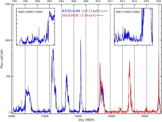
Figure 1: Daily averaged count rate (in mCrab) of RXTE/ASM (blue) in 1.5-12 keV energy band and MAXI/GSC (red) in 2-10 keV energy band.

2 Observation and data analysis

We use archival data of RXTE/ASM (in $1.5-12$ keV energy range) and MAXI/GSC (in $2-10$ keV energy range) for our study. Our analysis covers ten outbursts of GX 339-4. The daily average light curves are converted into Crab unit using proper conversion factors. The Crab conversion factor $75$ Counts/s for the ASM data ($1.5-12$ keV energy range) and $2.82$ photons cm^-2 s^-1 for GSC data ($2-10$ keV energy range) are used. For the analysis, we followed the same procedure as described in CDN19.

The nature of the outbursts is different from each other. The light curve of each outburst consists of multiple peaks. To fit each peak within an outburst, we use the Fast Rise and Exponential Decay (FRED) profile (Kocevski et al. 2003) as a model written in the ROOT data analysis framework of CERN. So to obtain the best fit, we require multiple FRED profiles. The combined FRED fit gives us total energy release i.e., the integrated flux of each outburst. As in CDN19, here we also used $12$ mCrab flux value as an outburst threshold to calculate the outburst duration.

According to Nandi et al. (2012 and references therein), one could get a rough idea about the spectral nature of the source from the evolution of hardness ratios (HRs; ratio of hard to soft X-ray flux or count rates). GX 339-4 showed all four usual spectral states (HS, HIMS, SIMS and SS) during its outbursts except those in $2013$, $2017-18$, and $2018-19$. To calculate the softer state (combined SIMS and SS) duration, we used the ratio of $5-12$ keV to $1.5-5$ keV ASM fluxes as HR for RXTE/ASM data and for MAXI/GSC HR, we used the ratio of $4-10$ keV to $2-4$ keV fluxes. Low and roughly constant HR values in the middle phase of the outbursts lead to the determination of the softer state duration. In case of the ‘failed’ outbursts of $2013$ and $2017-18$, the softer state duration dictates the SIMS duration only since in these two outbursts the SS are missing. In case of the mini outburst of $2018-19$ both the softer states (SIMS and SS) were missing in the HR diagram.

3 Results

A comparative study of the light curves of different sources and the energy release in each outburst helps one to understand the relation between the outburst and quiescence phases of black hole X-ray binaries (BHXRBs). Here we study the light curve profiles of the BHC GX 339-4. We fit the light curve of all the outbursts with multiple FRED profiles. From the FRED fitted curves, we calculate the integrated X-ray flux (IFX) in each outburst and make a comparative study. The fits also provide us with peak flux and duration (in MJD) of each outburst. Furthermore, we calculate the softer state duration in each outburst from the HR variations and the IFX during softer states (using FRED fitted curve). We also examine the relation of peak flux value with softer state IFX and softer state duration.

3.1 The Outburst Profile and Integrated Flux Calculation

Figure 1 shows the RXTE/ASM $1.5-12$ keV light curve (online blue) of GX 339-4 from January 1996 to June 2011 and the MAXI/GSC $2-10$ keV light curve (online red) starting from August 2009 to July 2020. The 2013 (Fürst et al. 2015) and the $2017-18$ (Garcia et al. 2019) outbursts were reported as ‘failed’ outbursts, as the source failed to make state transition into the SS. The $2018-19$ outburst was also a very short duration ‘failed’ in nature (Paice et al. 2019). Figure 1 shows that the peak flux reached maximum value during the $2006-07$ outburst and the peak flux value was minimum during the mini outburst of $2018-19$.

In Fig. 1, we show zoomed pre-outburst periods of the $1997-99$ outburst (MJD=50000 to MJD=51000) in the upper-left corner and $2006-07$ outburst (MJD=53600 to MJD=54260) in the upper-right corner. In the case of the $1997-99$ outburst, we can easily see that there are multiple small flaring activities before this outburst. Similarly, in $2006-07$ outburst, there is also one significant small flaring activity (MJD=53778 to MJD=53886) before the outburst.

As mentioned earlier, we use multiple FRED profiles to fit the RXTE/ASM and MAXI/GSC light curves in all the outbursts of the BHC GX 339-4. The shape of the light curve is described by the formula (Kocevski et al. 2003),

$$F(t)=F_{m}\left(\frac{t}{t_{m}}\right)^{r}\left[\frac{d}{d+r}+\frac{r}{d+r}\left(\frac{t}{t_{m}}\right)^{r+1}\right]^{-\frac{r+d}{r+1}},$$

where $F_{m}$ is the peak value of flux and $t_{m}$ is the time at which light curve has peak value of flux. Here ‘r’ denotes the rising index and ‘d’ denotes the decaying indices.

Figure 2: FRED profile fitting on $2010-11$ outburst data. The blue (online) curve is the total FRED fitted curve and the red (online) curves are FRED model fitted individual peaks. The flux value of 12mCrab was taken as the quiescent value for all outbursts. A horizontal line (black) with value of 12mCrab is drawn. The points where the total FRED-fitted curve (blue) touches the 12mCrab line are the start (in rising phase) and end (in declining phase) of the outburst. Beginning and end of the outburst are shown as the intersection points of the horizontal line with two vertical black lines in the rising and declining phases. Here, MJD=55149.5 is used as 0th day ($t_{0}$).

Figure 2 shows the FRED profile (online blue) fitted outburst profile ($2010-11$ in this case), i.e., daily light curve (black lines with points). A large fluxctuation in the residual is due to sudden spikes or dips in the data. We use a combination of six FRED profiles to fit the profile of the $2010-11$ outburst. To confirm k-number (here six) of FRED profiles (here six) are required for the best fit of the multi-peaked outbursts, we used Bayesian Information Criterion (BIC) selection method. $k\pm n$ (n=1,2,..) FRED model fits are excluded based on the threshold $\Delta(BIC)>8$.

During the quiescent state, the outbursts have a flux equivalent to a few mCrab. A limit of 12 mCrab is used as the threshold for the outbursts and energy release above this limit is integrated to measure the integrated flux (IFX) released per outburst. After getting the best fit of the outbursts with the FRED model, we mark the start and the end of an outburst based on the threshold flux chosen to be 12 mCrab as in CDN19. In Fig. 2, the horizontal line (black) shows the 12 mCrab flux value. The two vertical lines (black) mark the start and the end of the outburst. The IFX is calculated from the combined model fit. We also calculate various parameters, such as peak flux ($F_{m}$), peak time ($t_{m}$) and duration of the outburst from the combined FRED fitted curve. The similar fits are done for all outbursts and obtained parameters are provided in Table 1. From the $t_{m}$ values of the outbursts, the periods of accumulation of matter from the companion on the disk, as measured from the duration between the peaks of two successive outbursts, are also calculated for each outburst. In Table 2, FRED profile fitted paramters, integral flux and duration of each peak (online red curves) of the outbursts are tabulated. The duration and IFX values are calculated within 12 mCrab flux threshold of the individual model fitted curves. We also checked wheater the sum of the individual IFXs matches with the total integral flux (online blue curve) of the outburst.

Figure 3: (a) The histogram of the normalized flux per day of each outburst. The width of each histogram shows the duration of the outburst. (b) The normalized flux per day of the accumulation period for each outburst. All integrated fluxes are being normalized using the $2010-11$ integrated flux value. For the $1997-99$ outburst, the previous outburst is taken in 1995 (Rubin et al. 1998). (c) The normalized flux per day of the accumulation period for each outburst where the contribution from 2013 outburst is transferred into the $2014-15$ outburst, the contribution of the $2017-18$ and $2018-19$ is transferred to the $2019-20$ outburst.

From the obtained archival data of RXTE/ASM and MAXI/GSC, the count rates or fluxes and the corresponding uncertainties are converted into mCrab unit using conversion factors. We formed three data sets for each outburst: $(i)$ Set-I, MJD vs. flux values, $(ii)$ Set-II, MJD vs. error added flux value and $(iii)$ Set-III, MJD vs. error subtracted flux value. We fitted these three data sets for each outburst with FRED model and calculated peak flux ($F_{m}$), peak time ($t_{m}$), duration, the integrated flux value (IFX), the integrated flux value during softer states of outburst from the combined FRED fitted curve. We got the value of the variables from each of the three data sets. We calculated the differences of the main value (Set-I) with error added value (Set-II) and main value (Set-I) with error subtracted value (Set-III) of each variable obtained from these three data sets. By averaging those, we got the ‘$\pm$’ errors in each of the variables.

In Fig. 1, we see that the $2010-11$ outburst was observed by both RXTE/ASM and MAXI/GSC instruments. The values of the variables calculated from both RXTE/ASM and MAXI/GSC data are very close to each other (given in Table 1). The value of IFX calculated from RXTE/ASM data for the $2010-11$ outburst is 103371 mCrab day and the value of IFX calculated from the MAXI/GSC data is 103829 mCrab day. Due to less noise in the GSC data, we have taken 103829 value (the value of IFX of $2010-11$ outburst calculated from MAXI/GSC data) as a reference to normalize all the other outbursts.

We observed some peculiarities in the $2013$ and $2014-15$ outbursts. The 2013 outburst has a small peak flux of $\sim 51.58$ mCrab and minimum duration of $\sim 84$ days. The accumulation period for the 2013 outburst is very high ($\sim 1228$ days) compared to other outbursts of GX 339-4. In the immediate next outburst i.e., in $2014-15$, although the accumulation period is small ($\sim 554$ days), it showed a higher peak flux ($\sim 619$ mCrab) and a longer outburst duration of $\sim 352$ days. The same peculiarity can be seen in case of the $2017-18$, $2018-19$ and the $2019-20$ outbursts. In case of the $2017-18$ outburst, there is a large accumulation period of $\sim 1008$ days but the outburst duration is small ($\sim 173.1$ days) and a small peak flux value of $58.5$ mCrab. Whereas the $2019-20$ outburst has a small accumulation period of $\sim 314$ days but the outburst has a high peak flux value of $800$ mCrab. Possible reason of this behaviour would be discussed in the following sub-Sections.

For each outburst, we also calculated the value of IFX by simply integrating the flux values and calculated the normalized IFX w.r.t. the integral flux value of $2010-11$ outburst (given in the Table 1). We noticed that the IFX values from the simple integration method does not differ much with that of the FRED fits. But, the use of FRED model is more scientific way to find integrated flux and other parameters (peak flux, peak time, duration, etc) of the outbursts. Though, we have downloaded daily average ASM and GSC count rate/flux data from the archive, but data for some days are missing. Sometimes there are also sudden rise or dip in the light curves for one or two observations. We feel that these are the data errors. So, determination of the parameters without fitting with FRED profile will not give the information correctly. Thus, we use the value of the parameters that we get from the FRED fitted curve of each outburst for our analysis.

Figure 4: The possible flow dynamics in case of normal outbursts (a-b) and in case of failed outbursts (c-d).

3.2 A comparative study of outburst fluxes

The count rates of one day average data from RXTE/ASM and MAXI/GSC are converted to mCrab unit with proper conversion factors (mentioned above). Then all the outbursts are fitted with the multiple FRED profiles and the total integrated flux during each outburst is calculated in ‘mCrab day’ unit. We sub-divided the IFX of each outburst by the reference value of IFX of the $2010-11$ outburst (observed by MAXI/GSC) to get the normalized IFX in each outburst.

Figure 3(a) shows the IFX per day of outburst, normalized with respect to $2010-11$ outburst (normalized flux per day of an outburst). In Fig. 3(a), the area of each histogram represents IFX of each outburst and the width of each histogram represents the duration of each outburst. This IFX can be converted into the total energy release rate (Yan & Yu, 2015) using the prescription provided in http://xte.mit.edu.

Figure 3(b) shows the normalized IFX per day in the accumulation period of each outburst. For $1997-99$ outburst, the previous outburst is taken in 1995 (Rubin et al. 1998) and the peak flux value is taken on MJD=49955. We see that normalized flux per day of accumulation is roughly constant except for the outbursts during and after $2013$. In this Figure, we see that the normalized flux per day of accumulation is very low at $2013$, $2017-18$ and $2018-19$ outbursts. In case of the $2014-15$ outburst, the normalized flux per day of accumulation is the highest (much higher than the average line). In case of the $2019-20$ outburst the value of normalized flux per day of accumulation is also high. However, if the supply rate from the companion is almost constant, one might imagine that the energy release rate should remain almost the same for all the outbursts.

In order to resolve this anomaly, we may conjecture that perhaps $2013$ outburst did not release its entire accumulated matter and the leftover was released in $2014-15$ along with its normal release. This could be tested by adding the energy released in $2013$ and $2014-15$ outbursts and distribute the total energy emission rate from 2011 to 2014 evenly. After this exercise, we find that the average energy release in $2014-15$ outburst comes down to the average level as par with other outbursts (Fig. 3c). A similar situation occurred during the 2003 outburst of the BHC H 1743-322 as well. Physically, we believe that due to the lack of significant viscosity which triggered the 2013 outburst, only a part of the matter accumulated at the pile up radius could accrete. The rest joined with the matter piled up subsequently and when the viscosity was high enough, the 2014-2015 outburst started. In CDN19 a general cartoon diagram was presented to describe the flow behaviour in H 1743-322 and we believe exactly the same flow dynamics is occurring here as well. Just similar to the $2013$ outburst, the $2017-18$ outburst was also ‘failed’ in nature and the leftover matter of these outbursts were released in the successive outbursts i.e., in $2018-19$ (mini outburst) and $2019-20$ (main outburst). We combined the energy released in these three outbursts and treated them to be the parts of a single outburst (see, Fig. 3c). From the Fig. 3c, it is also evident that as time passed, the normalized IFX per day of accumulation was showing a decreasing trend, particular after the $2010-11$ outburst. It implies that there could be a non-constant rate of supply of matter from the companion.

In Fig. 4, we show what happens to a failed outburst as opposed to a complete normal outburst. Let us start with the configuration in the quiescence state (Fig. 4a). After the matter from the companion crosses the Roche-Lobe and creates an accretion shock, the flow continues to move inward till viscosity allows it to remain Keplerian (black annulus). The Keplerian disk halts at the pile-up radius $X_{p}$ (deep grey ring) where matter continues to pile up. Inside this radius, the hot, advective sub-Keplerian matter continues to flow emitting a little X-ray in this state. When the piled up matter becomes unstable and possibly larger convective viscosity drains out this accumulated matter completely and gradually, the outburst is triggered and reaches the final SS state via HS, HIMS and SIMS state and the Keplerian disk reaches the inner stable orbit (Fig. 4b). In a failed outburst, the disk may start in the same way (Fig. 4c). However, a significant viscosity may not be sustained for a long time, and the Keplerian disk may not move in all the way to the marginally stable orbit. Only a fraction of the piled-up matter will be depleted to produce the TCAF and due to the lower viscosity, the CENBOL does not reach the marginally stable orbit. In that case, the outburst will see at most in hard intermediate states or soft intermediate states (Fig. 4d). Due to partial evacuation of matter at pile-up radius, the rest of the matter remains there and gets added up with newly supplied matter from the companion which is released in the next outburst.

3.3 Calculation of softer state duration

Figure 5: Variation of (a) 2-10 keV MAXI/GSC lightcurve of the 2010-11 outburst and (b) hardness ratio (4-10 keV/2-4 keV count rate) as a function of the Modified Julian Day (MJD). The start and the end of the softer state are shown with two vertical dashed lines.

To understand the accretion dynamics and the radiative properties of a BHC, one needs to study both the spectral and temporal properties of the source. The variation of the hardness ratio (HR; the ratio between fixed energy hard and soft band photon counts) provides us with a rough idea to understand spectral nature and transition dates during an outburst of a transient BHC. Since in HR, we use two fixed energy band photon rates/fluxes, transition dates between the spectral states may not be same, i.e., may differ slightly when we confirm from the spectral analysis with phenomenological (for e.g., disk black body plus power-law models) or physical models, such as TCAF solution, developed by Chakrabarti and his collaborators (Chakrabarti & Titarchuk 1995; Chakrabarti 1997). TCAF model has successfully designated the spectral states of many black hole candidates during their outbursts (Nandi et al. 2012; Debnath et al. 2013, 2014, 2015a,b, 2017, 2020; Mondal et al. 2014, 2016; Chatterjee et al. 2016, 2019, 2020; Jana et al. 2016, 2020; Shang et al. 2019). However, according to literature (see for example, Debnath et al. 2008; Nandi et al. 2012 and references therein) it is believed that in the harder states HR values are higher and in the softer states HR values are low. More distinctly in HS, HR values are roughly constant with high value and in HIMS, HR changes rapidly. In the rising HIMS period, HR reduces rapidly and in the declining HIMS, HR increases rapidly. In the softer spectral states (SIMS and SS), we see low values of HRs in the middle phase of the outburst, where soft disk black body flux or Keplerian disk photons dominate.

Figure 5(a) shows the 2-10 keV MAXI/GSC lightcurve of $2010-11$ outburst. The corresponding time evolution of the hardness ratio (HR; the ratio of photon fluxes in $4-10$ keV and $2-4$ keV bands) is plotted in Fig. 5(b). The origin of the time axis is at 2009 Oct. 26 (MJD=55130). We see that HR has a high value at the beginning of the outburst. After some time it gradually decreases. Subsequently, for a comparatively long time (from MJD=55308.4 to MJD=55584.9) the value remains almost the same. Then the HR again increases gradually to a high value. Variation of the hardness ratio distinctly shows the state transitions from harder to softer spectral states. During the middle region of the outburst, low HR values are observed, which corresponds to the softer spectral states. Two dashed vertical lines show the start and end of the softer states. For this $2010-11$ outburst, the softer state starts on MJD=55308.4 and ends on MJD=55584.9 with a duration of $276.5$ days. A similar analysis is done to calculate softer state durations of all other outbursts of GX 339-4. The results are provided in Table 1.

Figure 6: The correlation in between (a) the peak flux value and the duration of softer states, (b) the peak flux value and normalized integrated X-ray flux (IFX) during softer state. In both the figures the RXTE/ASM data points are denoted by diamonds and the MAXI/GSC data points are denoted by circles. The outbursts of $1997-99$, $2006-07$ and $2019-20$ are marked as online red since they do not follow the general trend as the other outbursts.

3.4 Peak flux relation with softer states

Here we attempt to find the correlation between the peak flux values ($F_{m}$) of the outburst, obtained from FRED profile fits and softer state durations during the GX 339-4 outbursts. We calculated the peak flux value from the outburst profile of each outburst, and the softer state duration from the evolution of the HR. In Fig. 6(a), we plot the peak flux value ($F_{m}$) vs. softer state duration. The better the linear regression fits the data, the closer the value of R-square is to $1$ and a correlation is statistically significant if the P-value is less than $0.05$ (typically $\leq 0.05$). For the correlation in between $F_{m}$ and softer state duration the values of R-squared and P-value are obtained $0.923$ and $0.002$ respectively. We also calculated the integrated flux during the softer state ($IFX_{softer}$) of each outburst and normalized them with respect to the $IFX_{softer}$ of the $2010-11$ outburst. Figure 6(b) shows the peak flux value ($F_{m}$) vs. the normalized IFX in softer states ($IFX_{softer}$). The R-squared value and P-value for the correlation in between $F_{m}$ and $IFX_{softer}$ are 0.960 and 0.0006 respectively. We found linear relations in both the plots (Fig. 6a & 6b). But the outbursts of $1997-99$, $2006-07$ and $2019-20$ do not follow this linearity condition.

The peak flux is decided by the maximum supply of the Keplerian matter, i.e., when the viscosity of the accretion disk is maximum. After that, the viscosity is turned off and supply of the disk matter from the pile-up radius is reduced, triggering the onset of the declining phase. The larger the value of the peak flux, the longer it takes to wash out the Keplerian matter after the viscosity is turned off (Roy & Chakrabarti 2017). In Roy & Chakrabarti (2017), theoretically, it is done by mixing Keplerian and sub-Keplerian halo components and then draining the mixture. Otherwise, it is difficult to drain the high angular momentum Keplerian matter from the system as the viscosity is reduced. Thus, the source remains in the softer states (SS and SIMS) for a long time. So, there is a correlation between the peak flux value (maximum viscous day) with the $IFX_{softer}$ and the duration of the softer states. In Figs. 6(a) & 6(b), we see a general trend of a linear relation between these. However, in both the Figures, we see that the $1997-99$, $2006-07$ and $2019-20$ outbursts (marked as online red) do not follow the general trend as the other outbursts. When we examine the profiles of the $1997-99$ and $2006-07$ outbursts, we see that just before the start of these two outbursts there were many smaller flaring activities, which may have depleted some of the accumulated matter at the pile-up radius (see zoomed insets containing the pre-outburst phase in Fig. 1). Multiple small flaring activities before the $1997-99$ outburst was reported earlier (Zdziarski et al. 2004). In the case of $2006-07$ outburst, there was a very small outburst during MJD $53751-53876$ (Buxton et al. 2012). In prior to the $2019-20$ outburst, there was two ‘failed’ outbursts; the 2017-18 outburst and a mini outburst ($2018-19$ outburst). These two outbursts might be the reason for which the $2019-20$ outburst did not follow the linear relation as shown in Fig. 6(a) and 6(b).

4 Discussion and conclusions

In the post RXTE era (1996 onwards) the source GX 339-4 showed several outbursts at irregular intervals of $2-3$ years. The nature of each of these outbursts is different. There are differences in duration, accumulation period (Quiescence phase), maximum peak intensity, etc. in these outbursts. Recently, Chakrabarti and his collaborators were quite successful to find out the physical reason behind the variation of the nature of outbursts of the Galactic transient H 1743-322 (see, CDN19). They found a relation between the energy release at an outburst and the duration between the current and the previous peak times.

The supply of matter from the companion via Roche-lobe overflow continues in rising as well as the declining and quiescence phases. Generally, an outburst is triggered when viscosity rises above a critical value and the declining phase starts when the viscous effect is turned off (see, Chakrabarti et al. 2005 and references therein). Matter from the outer disk inside the Roche-lobe of the accretor may not be able to form a Keplerian disk till the marginally stable orbit due to lack of significant viscosity. Initially, due to low viscosity, this matter starts to accumulate at a location, far away from the black hole, known as pile-up radius ($X_{p}$). With an increase in the amount of accumulated matter, the thermal pressure rises. As a result, turbulence and instability increases, which in turn increases the viscosity above the critical value. With this high viscosity, matter rushes towards the black hole in both Keplerian and sub-Keplerian components (TCAF) from $X_{p}$ and triggers an outburst. While releasing most of the stored hot matter at the pile-up radius ($X_{p}$), the viscosity is turned off triggering an onset of the declining phase followed by the quiescent state. The quiescence phase duration varies with $X_{p}$. For larger $X_{p}$, the quiescence phase duration is also high because, a larger value of $X_{p}$ requires higher viscosity to trigger the outburst, i.e., more accumulation of matter is required, resulting in larger duration of quiescence. Some examples were given in CDN19. The matter accumulated at $X_{p}$ from the peak day of the previous outburst up to the peak day of the ongoing outburst contributes to the current outburst. Thus the total energy released in an outburst reflects the amount of matter accumulated at the pile-up radius during the accumulation period prior to that outburst.

The relation between the outbursts and quiescence periods are also studied for the Galactic transient GX 339-4. To calculate accumulation duration of the matter at $X_{p}$, we considered peak (of the previous outburst) to peak (of the considering outburst) durations, which also include the quiescence periods. We notice that the average energy release in an outburst is proportional to the period of accumulation just prior to it, with the exception of the outbursts which occurred in $2013$, $2014-15$, $2017-18$, $2018-19$ and $2019-20$. We found that the 2013 and $2017-18$ outbursts were ‘failed’ outbursts where the energy released were not complete. If we combine the energies released at the 2013 and $2014-15$ outbursts and treat them to be the parts of a single outburst, then the linear relation could be seen. The possible flow dynamics in a normal and failed outbursts are shown in Fig. 4. In Fig. 4(c-d), only a part of the matter is released as in 2013 outburst. The leftover matter at the pile-up radius was combined with freshly supplied matter from the companion and produced the normal outburst of $2014-15$ with higher than the expected flux. Similar to the $2013$ outburst, the $2017-18$ is also an incomplete outburst. We also found that the $2019-20$ outburst released more than its share as in $2014-15$ outburst. There was also a mini outburst of $2018-19$ in between the $2017-18$ and $2019-20$ outbursts. We combined the energies released in the three successive outbursts of $2017-18$, $2018-19$ and $2019-20$, and treated them to be the parts of a single outburst that took place in $2019-20$.

We also show the relationship between the peak flux ($F_{m}$) and softer (SIMS and SS) states. When we plot the peak flux ($F_{m}$) vs. softer state duration (Fig. 6a) and peak flux vs. normalized integrated flux in softer states (Fig. 6b), we find a linear correlation in both the plots. The peak flux value indicates the amount of matter accumulated during the rising phase, and which clears out during softer states. So, the higher the value of the peak flux, the larger is the value of the softer states’ duration. Although, in both Figs. 6(a-b), the outbursts $1997-99$, $2006-07$ and $2019-20$ do not show similar trends as in other outbursts of GX 339-4. We found a possible reason for this anomalous behaviour. It seems that prior to both of these main outbursts, piled up matter was ‘leaking’ and gave rise to some weaker flares even in the so-called quiescence phase. In CDN19, they proposed that the 2003 outburst of the BHC H 1743-322 stopped prematurely. The following outburst of 2004 released the remaining part of the energy that was due to be released in 2003 outburst. The matter accumulated at the pile up radius before the 2003 outburst could not get cleared during the 2003 outburst but remained stuck at a nearer pile up radius. After 2003 outburst, more matter accumulated at the new pile up radius and triggered the subsequent 2004 outburst. The duration of the 2003 outburst was 230.5 days, and the duration of the 2004 outburst was 112.2 days. As the pile up radius prior to 2004 outburst ($X_{p2004}$) was closer (to BH) than the pile up radius prior to outburst of 2003 ($X_{p2003}$), the duration of 2004 outburst was smaller than the outburst of 2003. In case of the outburst of $2006-07$ and $2019-20$ of the BHC GX 339-4, a small softer state duration was observed (see, Fig. 6). During the small ‘failed’ outbursts prior to these two outbursts, matter started to rush from the pile up radius ($X_{pfailed}$) towards the black hole but due to sudden fall in viscosity, a large part of the infalling matter stopped prematurely and remained stuck at a new pile up radius nearer to the BH. Freshly accreted matter from the companion was also accumulated at the new pile up radius and gave rise to the viscosity. When the viscosity raised sufficiently, these accumulated matter at the new pile up radius, started to fall towards the black hole again and produced the main outburst. Since the pile up radii in these two cases i.e., prior to the main outbursts of $2006-07$ and $2019-20$ are nearer to the BH ($X_{pmain}<X_{pfailed}$), thus the duration of these two outbursts were small. If the pile up radius is nearer to the BH, relatively less accumulation of matter is required to trigger the outburst, since the disc is hotter and ionized there. As the duration of these two outbursts were small, softer state durations were also shorter. That is why these two outbursts are outlier in Fig. 6a and 6b. In case of the $1997-99$ outburst, we are unable to properly predict and discuss the accumulation location and accretion flow as there was lack of sufficient data before the start of the outburst. On the eve of this outburst, only some small flaring activities are seen. What happened before that is not clear from the data. Beside inward shift of the pile up radius due to the failed outbursting attempts prior to the main outburst, outburst duration as well as softer state duration and integrated flux during softer state of the present source, also influenced by the non-constant rate of mass supply from the companion. It is evident from the Fig. 3c that Normalized flux per day of the accumulation period showed a decreasing trend as time passed, particularly after the 2010-11 outburst. This means that supply rate from the companion seems to have decreased as the day progressed. In the near future, GX 339-4 may proceed to a long duration quiescence phase.

In any case, our global picture of accumulation of matter at the pile-up radius and its release rate as per availability of viscous processes hold good for the present source. This was also seen to be the case in outbursts of H 1743-322. In future we will verify the findings of our work with other transient BHCs and the results would be reported elsewhere.

Table 1: Peak data and normalized integrated X-ray flux (IFX) during outbursts of GX 339-4

Outburst	Peak Day	Peak flux	Duration	Accumulationa	Normalized IFX	Normalized IFXb	Softer state	Normalized IFX of
Year				Period	w.r.t.	w.r.t. $2010-11$	duration	softer state w.r.t.
	(MJD)	(mCrab)	(Days)	(Days)	$2010-11$	(simple integration)	(Days)	$(2010-11)$
RXTE/ASM
$1997-99$	50873.5	$305.5\pm 33.5$	686.0	918.5	$0.946\pm 0.061$	$0.951\pm 0.094$	$348.6\pm 45.5$	$0.925\pm 0.078$
$2002-03$	52495.5	$877.8\pm 9.6$	454.3	1622.0	$1.519\pm 0.066$	$1.522\pm 0.096$	$312.3\pm 0.90$	$1.620\pm 0.003$
$2004-05$	53303.4	$484.4\pm 11.5$	446.7	806.9	$0.750\pm 0.050$	$0.757\pm 0.072$	$230.5\pm 3.60$	$0.760\pm 0.033$
$2006-07$	54152.8	$972.0\pm 5.5$	232.6	849.8	$0.490\pm 0.059$	$0.482\pm 0.038$	$89.90\pm 1.50$	$0.428\pm 0.016$
$2010-11$	55308.2	$689.8\pm 10.2$	401.9	1156.6	$0.995\pm 0.007$	$0.986\pm 0.067$	$274.2\pm 5.12$	$0.999\pm 0.026$
MAXI/GSC
$2010-11$	55308.5	$708.1\pm 14.7$	399.2	1156.3	$1.000\pm 0.051$	$1.00\pm 0.076$	$276.5\pm 6.30$	$1.000\pm 0.046$
2013	56536.9	$51.58\pm 3.5$	84.0	1228.4	$0.029\pm 0.007$	$0.028\pm 0.006$	$51.10\pm 5.10^{*}$	$0.025\pm 0.004$
$2014-15$	57090.7	$619.3\pm 12.5$	352.1	553.8	$0.735\pm 0.041$	$0.737\pm 0.069$	$192.1\pm 15.4$	$0.850\pm 0.045$
$2017-18$	58098.7	$58.5\pm 10.9$	173.1	1008.0	$0.047\pm 0.012$	$0.049\pm 0.011$	$92.90\pm 6.90^{*}$	$0.039\pm 0.008$
$2018-19$	58530.5	$29.43\pm 10.8$	115.7	431.8	$0.022\pm 0.012$	$0.025\pm 0.010$	$------$	$------$
$2019-20$	58844.1	$799.5\pm 15.1$	238.9	313.6	$0.335\pm 0.023$	$0.336\pm 0.037$	$71.0\pm 9.00$	$0.191\pm 0.011$

^a Accumulation period is taken from the peak day of previous outburst to the concerned outburst.

^∗ In case of $2013$ and $2017-18$ outbursts the softer state duration dictates the SIMS duration only.

^b Integral flux is obtained by simple integration method and then normalized w.r.t. the integral flux of $2010-11$ outburst.

Table 2: FRED Profile Fitted Parameters, Integral flux values and Duration in Each Peak of the GX 339-4 Outbursts

Outburst	K	K1	K2	K3	K4	K5	K6	K’s Integral Flux	K’s Duration
(1)	(2)	(3)	(4)	(5)	(6)	(7)	(8)	(9)	(10)
1997-99	5	35.4, 50673,	49.6, 50729,	197, 50867,	263, 51029,	18.9, 51246,	- - -	6299, 1148, 190003,	202, 31.0, 227,
		0.755, 5.39	15.2, 86.4	13.3, 7.46	3.48, 8.2E+6	378, 10.6	- - -	70090, 814	516, 35.8
2002-03	4	291, 52386,	498, 52411	871, 52496,	213, 52650,	- - -	- - -	12623, 10235,	116, 59,
		43.8, 11.0	81.3, 28.8	11.6, 8.06	23.02, 57.7	- - -	- - -	120089, 14760	448, 142
2004-05	3	62.3, 53095,	481, 53303,	126, 53434,	- - -	- - -	- - -	4755, 63259, 9851	115, 339, 139
		3.86, 4.20	7.68, 10.02	13.54, 1.1E+7	- - -	- - -	- - -
2006-07	3	157, 54124,	942, 54154,	19.52, 54220,	- - -	- - -	- - -	7598, 42395, 867	90, 179, 33.9
		6.74, 17592	30.9, 7.32	13.40, 1.1E+7	- - -	- - -	- - -
2010-11	6	260, 55307,	446.9, 55309,	287, 55375,	205, 55450,	232, 55510,	85.8, 55570,	19054, 27898, 22757,	146, 264, 220,
		4.9, 1.1E+6	76.8, 3.87	20.5, 6.19	11.8, 6.9E+6	13.9, 202	17.5, 1.2E+7	13094, 15718, 5308	126, 138, 100
2013	1	51.6, 56536,	- - -	- - -	- - -	- - -	- - -	2972.92	83.98
		1.17, 2.6E+6	- - -	- - -	- - -	- - -	- - -
2014-15	5	86.5, 57005,	393, 57042,	488, 57095,	180, 57163,	117, 57240,	- - -	4758, 21833, 37099,	90.7, 228, 182,
		5.75, 62.6	151, 4.2	8.92, 20.8	40.2, 9.97	58.5, 92.9	- - -	10105, 2569	132, 39.2
2017-18	3	34.7, 58044,	56.5, 58100,	48.5, 58178,	- - -	- - -	- - -	1804, 2619, 416	64.3, 66.5, 12.5
		1.6, 1.5E+6	10.4, 6.67	109, 45.6	- - -	- - -	- - -
2018-19	2	20.9, 58478,	22.6, 58533,	- - -	- - -	- - -	- - -	1402, 885	63.4, 42.4
		0.935, 4.7E+6	15.9, 3.09	- - -	- - -	- - -	- - -
2019-20	5	37.4, 58769,	463, 58848,	348, 58844,	82.8, 58879,	133, 58902,	- - -	2475, 20149, 3860,	83.3, 96.3, 37.8,
		1.62, 34.9	7.55, 1.3E+7	954, 13.7	151, 6.87	22.5, 11.2	- - -	2582, 5759	61.0, 88.1

In Col. 2, K denotes the number of FRED models used to fit the entire outburst.

K1-K6 mark individual model fitted parameters: peak flux ($F_{m}$ in $mCrab$), peak day ($t_{m}$ in MJD), rising index ($r$), decaying index ($d$).

Col. 9 & 10 mark integral flux and duration of the individual peaks in units of $mCrab~{}day$ and $day$ respectively.

References

- Buxton et al. (2012) Buxton, M. M., Bailyn, C. D., Capelo, H. L., & Chatterjee, R., 2012, AJ, 143, 130B
- Chakrabarti & Titarchuk (1995) Chakrabarti, S. K., & Titarchuk, L. G., 1995, ApJ, 455, 623
- Chakrabarti (1997) Chakrabarti, S. K., 1997, ApJ, 484, 313
- Chakrabarti et al. (1989) Chakrabarti, S. K., 1989, MNRAS, 240, 7
- Chakrabarti et al. (1990) Chakrabarti, S. K. 1990, Theory of Transonic Astrophysical Flows (Singapore: World Scientific)
- Chakrabarti et al. (2005) Chakrabarti, S. K., Nandi, A., Debnath, D., et al. 2005, IJP, 79, 841 (arXiv: astro-ph/0508024)
- Chakrabarti et al. (2015) Chakrabarti, S.K., Mondal, S., & Debnath, D., 2015, MNRAS, 452, 3451
- Chakrabarti et al. (2019) Chakrabarti, S. K., Debnath, D., & Nagarkoti, S., 2019, AdSpR, 63, 3749
- Chatterjee et al. (2016) Chatterjee, D., Debnath, D., Chakrabarti, S. K., Mondal, S., Jana, A., 2016, ApJ, 827, 88
- Chatterjee et al. (2019) Chatterjee, D., Debnath, D., Jana, A., & Chakrabarti, S. K., 2019, ApSS, 364, 14
- Chatterjee (2020) Chatterjee, K., Debnath, D., Chatterjee, D., et al. 2020, MNRAS, 493, 2452
- Cowley et al. (2002) Cowley, A. P., Schmidtke, P. C., Hutchings, J. B., & Crampton, D., 2002, AJ, 123, 1741
- Debnath et al. (2008) Debnath, D., Chakrabarti, S. K., Nandi, A., et al., 2008, BASI, 36, 151
- Debnath et al. (2013) Debnath, D., Chakrabarti, S. K., & Nandi, A., 2013, Adv. Space Res., 52, 2143
- Debnath et al. (2014) Debnath, D., Chakrabarti, S. K., Mondal, S., 2014, MNRAS, 440, L121
- Debnath et al. (2015a) Debnath, D., Mondal, S., & Chakrabarti, S. K., 2015a, MNRAS, 447, 1984
- Debnath et al. (2015b) Debnath, D., Molla, A. A., Chakrabarti, S. K., Mondal, S., 2015b, ApJ, 803, 59
- Debnath et al. (2017) Debnath, D., Jana, A., Chakrabarti, S. K., Chatterjee, D., & Mondal, S., 2017, ApJ, 850, 52
- Debnath et al. (2020) Debnath, D., Chatterjee, D., Jana, A., Chakrabarti, S. K., & Chatterjee, K., 2020, RAA, 20, 175
- Ebisawa et al. (1996) Ebisawa, K., Titarchuk, L., & Chakrabarti, S. K., 1996, PASJ, 48, 59
- Furst et al. (2015) Fürst, F., Nowak, M. A., Tomsick, J. A., Miller, J. M., Corbel, S., et al. 2015, ApJ, 808, 122
- Garcia et al. (2017) Garcia, J. A., Harrison, F., Tomsick, J., et al. 2017, ATel, 10825
- Garcia et al. (2019) Garcia, J. A., Tomsick, J. A., Sridhar, N., et al. 2019, ApJ, 885, 48
- Heida et al. (2017) Heida, M., Jonker, P. G., Torres, M. A. P., & Chiavassa, A., 2017, ApJ, 846, 132
- Hynes et al. (2004) Hynes, R. I., Steeghs, D., Casares, J., Charles, P. A., & O’Brien, K., 2004, ApJ, 609, 317
- Jana (2016) Jana, A., Debnath, D., Chakrabarti, S. K., Mondal, S., Molla, A. A., 2016, ApJ, 819, 107
- Jana et al. (2020) Jana, A., Debnath, D., Chatterjee, D., et al. 2020, RAA, 20, 28
- Kocevski et al. (2003) Kocevski, D., Ryde, F., & Liang, E., 2003, ApJ, 596, 389
- Ludlam et al. (2015) Ludlam, R. M., Miller, J. M., & Cackett, E. M., 2015, ApJ, 806, 262
- Markert et al. (1973) Markert, T. H., Canizares, C. R., Clark, G. W., et al. 1973, ApJ, 184, 67
- Miller et al. (2008) Miller, J. M., Reynolds, C. S., Fabian, A. C., Cackett, E. M., et al. 2008, ApJ, 679, L113
- Nandi et al. (2012) Nandi, A., Debnath, D., Mandal, S., & Chakrabarti, S. K., 2012, A&A, 542, A56
- Molteni et al. (1996) Molteni, D., Sponholz, H., & Chakrabarti S. K., 1996, ApJ, 457, 805
- Mondal, Debnath & Chakrabarti (2014) Mondal, S., Debnath, D., & Chakrabarti, S. K., 2014, ApJ, 786, 4
- Mondal, Chakrabarti & Debnath (2016) Mondal, S., Chakrabarti, S. K., & Debnath, D., 2016, ApSS, 361, 309
- Paice et al. (2019) Paice, J. A., Gandhi, P. & Belloni, T., et al. 2019, ATel, 13264, 1
- Parker et al. (2016) Parker, M. L., Tomsick, J. A., Kennea, J. A., Miller, J. M., et al. 2016, ApJ, 821, L6
- Remillard & McClintock (2006) Remillard, R. A., & McClintock, J. E., 2006, ARA&A, 44, 49
- Roy & Chakrabarti (2017) Roy, A., & Chakrabarti, S. K., 2017, MNRAS 472, 4689
- Rubin et al. (1998) Rubin, B. C., Harmon, B. A., Paciesas, W. S., et al. 1998, ApJ, 492, 67
- Ryu et al. (1997) Ryu, D., Chakrabarti, S. K., & Molteni, D. 1997, ApJ, 474, 378
- Shang et al. (2019) Shang, J. R., Debnath, D., & Chatterjee, D., et al. 2019, ApJ, 875, 4
- Sreehari et al. (2019) Sreehari, H., Iyer, N., Radhika, D., Nandi, A., Mandal, S., 2019, AdSpR, 63, 1374S
- Tetarenko et al. (2016) Tetarenko, B. E., Sivakoff, G. R., Heinke, C. O., & Gladstone, J. C., 2016, ApJS, 222, 15
- Yan and Yu (2015) Yan, Z., & Yu, W., 2015, ApJ, 805, 87
- Zdziarski et al. (2004) Zdziarski, A. A., Gierlinski, M., Mikolajewska, J., et al. 2004, MNRAS, 351, 791