Accessible information of a general quantum Gaussian ensemble

Abstract

Accessible information, which is a basic quantity in quantum information theory, is computed for a general quantum Gaussian ensemble under certain “threshold condition”. It is shown that the maximizing measurement is Gaussian, constituting a far-reaching generalization of the optical heterodyning. This substantially extends the previous result concerning the gauge-invariant case, even for a single bosonic mode. A simple sufficient condition is provided that implies the threshold condition for general Gaussian ensemble. The results are illustrated on the single-mode case.

I Introduction

Accessible information of an ensemble of quantum states is a basic quantity in quantum information theory: it is equal to the maximal amount of the Shannon information which can be gained from a given quantum ensemble (a collection of “signal” quantum states with fixed probabilities) in a one-step measurement. This quantity is often difficult to compute, the problem lies in finding the global maximum of a convex functional, when the maximizer turns out to be highly non-unique and the standard tools of convex analysis become inefficient. The problem becomes still more complicated for continuous variable (CV) systems which constitute one of the prospective platforms for implementation of ideas of quantum information theory (see e.g. sera ). The quantum Shannon theory for CV systems requires mathematical tools of infinite-dimensional Hilbert spaces and symplectic vector spaces, see QSCI .

The present paper is a continuation and extension of our paper acc which gave a solution for the problem going back to 1970-s: it was shown there that accessible information of a gauge-invariant bosonic Gaussian ensemble is attained by a multimode generalization of heterodyne measurement, and hence can be computed exactly. (Loosely speaking, gauge invariance means that the problem has a unique natural complex structure. In quantum optics, this is related to phase-insensitivity of the system.)

In the present paper we extend this result to arbitrary Gaussian ensembles satisfying certain “threshold condition” . This condition is the one that allows to reduce the classical capacity problem to a simpler minimum output entropy problem, and it is always fulfilled in the particularly tractable gauge-invariant case. Thus we obtain here a “Gaussian maximizer” result in a situation going beyond gauge invariance (which is often assumed, see e.g. depalma , QSCI for various aspects of the famous “Gaussian optimizer conjecture” in analysis and quantum information theory). Main tools will be the infinite-dimensional version of “ensemble-observable duality” developed in acc and the multiplication formulas for Gaussian operators from lami (see also Appendix 1).

II Preliminaries

We refer reader to QSCI for definitions of basic notions of quantum statistics. Let $\mathcal{H}$ be a separable Hilbert space, $\mathcal{X}$ a standard measurable space. An ensemble $\mathcal{E}=\left\{\pi(dx),\rho_{x}\right\}$ consists of a probability measure $\pi(dx)$ on $\mathcal{X}$  and a measurable family of density operators (quantum states) $x\rightarrow\rho_{x}$ on $\mathcal{H}$. The average state of the ensemble is the barycenter of this measure

$$\bar{\rho}_{\mathcal{E}}=\int_{\mathcal{X}}\rho_{x}\,\pi(dx),$$

the integral existing in the strong sense in the Banach space of trace-class operators on $\mathcal{H}$. Let $M=\{M(dy)\}$ be an observable (probability operator-valued measure = POVM) on $\mathcal{H}$ with the outcome space $\mathcal{Y}$ . There exists a $\sigma-$finite measure $\mu(dy)$ such that for any density operator $\rho$ the probability measure $\mathrm{Tr}\rho M(dy)$ is absolutely continuous w.r.t. $\mu(dy),$ thus having the probability density $p_{\rho}(y)$ (one can take $\mu(dy)=\mathrm{Tr}\rho_{0}M(dy)$ where $\rho_{0}$ is a nondegenerate density operator).

The joint probability distribution of $x,y$ on $\mathcal{X\times Y}$ is uniquely defined by the relation

$$P(A\times B) = \int_{A}\pi(dx)\mathrm{Tr}\,\rho_{x}M(B)$$

$$= \mathrm{Tr}\int_{A}\int_{B}\,p_{\rho_{x}}(y)\,\pi(dx)\mu(dy),$$

where $A$ is an arbitrary Borel subset of $\mathcal{X}$ and $B$ is that of $\mathcal{Y}.$ The classical Shannon information between $x,y$ is equal to

$$I(\mathcal{E},M) = \int\int\pi(dx)\mu(dy)p_{\rho_{x}}(y)\log\frac{p_{\rho_{x}}(y)}{p_{\bar{\rho}_{\mathcal{E}}}(y)}$$

$$= h(p_{\bar{\rho}_{\mathcal{E}}})-\int h(p_{\rho_{x}})\pi(dx),$$

where

$$h(p)=-\int p(x)\log p(x)\mu(dx)$$

is the differential entropy of a probability density $p(x).$ There is a special class of probability densities we will be dealing with for which the differential entropy is well-defined (see acc for the detail).

The accessible information of the ensemble $\mathcal{E}$ is defined as

$$A(\mathcal{E}\mathbf{)=}\sup_{M}I(\mathcal{E},M),$$ (1)

where the supremum is over all observables $M$ on $\mathcal{H}$.

We will systematically use notations and results from the book QSCI . Consider the finite-dimensional symplectic space $(Z,\Delta)$ with $Z=\mathbb{R}^{2s}$ and

$$\Delta=\mathrm{diag}\left[\begin{array}[]{cc}0&1\\ -1&0\end{array}\right]_{j=1,\dots,s}.$$ (2)

In what follows $\mathcal{H}$ will be the space of an irreducible representation $z\rightarrow W(z);\,z\in Z,$ of the canonical commutation relations

$$W(z)W(z^{\prime})=\exp[-\frac{i}{2}z^{t}\Delta z^{\prime}]\,W(z+z^{\prime}).$$ (3)

Here $W(z)=\exp i\,Rz$ are the unitary Weyl operators with the generators

$$Rz=\sum_{j=1}^{s}(x_{j}q_{j}+y_{j}p_{j}),$$ (4)

$z=[x_{j}\,\,y_{j}]_{j=1,\dots,s}^{t}$, and $R=[q_{j}\,\,p_{j}]_{j=1,\dots,s}$ are the canonical observables of the quantum system in question satisfying $q_{j}p_{k}-p_{k}q_{j}=\delta_{jk}I$ . In quantum communication theory they describe the relevant modes of the field on receiver’s aperture (see, e.g. sera ). The displacement operators $D(z)=W(-\Delta^{-1}z)$ satisfy the equation that follows from the canonical commutation relations (3)

$$D(z)^{\ast}W(w)D(z)=\exp\left(iw^{t}z\right)W(w).$$ (5)

A centered Gaussian state $\rho_{\alpha}$ is determined by its quantum characteristic function

$$\mathrm{Tr}\,\rho_{\alpha}W(z)=\exp\left(-\frac{1}{2}z^{t}\alpha z\right),$$ (6)

where the covariance matrix $\alpha=\mathrm{Re\,}\mathrm{Tr}\,R^{t}\rho R$ is a real symmetric $2s\times 2s$-matrix satisfying

$$\alpha\geq\pm\frac{i}{2}\Delta.$$ (7)

Operator $J$ in $(Z,\Delta)$ is called operator of complex structure if

$$J^{2}=-I_{2s},$$ (8)

where $I_{2s}$ is the identity operator in $Z$, and it is $\Delta-$positive in the sense that

$$\Delta J=-J^{t}\Delta,\quad\Delta J\geq 0.$$ (9)

In other words, $\Delta$ is tamed by $J$.

The Gaussian state $\rho_{\alpha}$ is pure if and only if $\alpha=\frac{1}{2}\Delta J$ where $J$ is an operator of complex structure. Such state is called $J-$vacuum and denoted $\rho_{\frac{1}{2}\Delta J}.$ The non-centered pure states $D(z)\rho_{\frac{1}{2}\Delta J}D(z)^{\ast}$ are called $J-$coherent states (see sec. 12.3.2 of  QSCI ).

Consider the operator $A=\Delta^{-1}\alpha$. The operator $A$ is skew-symmetric in the Euclidean space $(Z,\alpha)$ with the scalar product $\alpha(z,z^{\prime})=z^{t}\alpha z^{\prime}$. According to a theorem from linear algebra, there is an orthogonal basis $\left\{e_{j},h_{j}\right\}$ in $(Z,\alpha)$ and positive numbers $\left\{\alpha_{j}\right\}$ (called symplectic eigenvalues of $\alpha$) such that

$$Ae_{j}=\alpha_{j}h_{j};\quad Ah_{j}=-\alpha_{j}e_{j},\quad j=1,\dots,s.$$

Inequality (7) is equivalent to $N_{j}\equiv\alpha_{j}-1/2\geq 0$, $j=1,\dots,s.$ Choosing the normalization  $\alpha(e_{j},e_{j})=\alpha(h_{j},h_{j})=\alpha_{j}$ gives a symplectic basis in $(Z,\Delta)$.

There is an operator of complex structure, commuting with the operator $A=\Delta^{-1}\alpha,$ namely, the orthogonal operator $J_{\alpha}$ from the polar decomposition

$$A=\left|A\right|J_{\alpha}=J_{\alpha}\left|A\right|$$ (10)

in the Euclidean space $(Z,\alpha).$ The action of $\left|A\right|$ and $J_{\alpha}$ in the symplectic basis $\left\{e_{j},h_{j}\right\}$ constructed above is given by the formula

$$\left|A\right|e_{j} = \alpha_{j}e_{j},\quad\left|A\right|h_{j}=\alpha_{j}h_{j};$$

$$J_{\alpha}e_{j} = h_{j},\quad\quad J_{\alpha}h_{j}=-e_{j}.$$

Inequality (7) is equivalent to

$$\alpha\geq\frac{1}{2}\Delta J_{\alpha}$$ (11)

because it amounts to $\alpha_{j}-1/2\geq 0$, $j=1,\dots,s.$

We will consider the general Gaussian observable (probability operator-valued measure = POVM) on $Z=\mathbb{R}^{2s}$ (see  acc )

$$\widetilde{M}(d^{2s}z)=D(Kz)\rho_{\beta}D(Kz)^{\ast}\frac{\left|\det K\right|\,d^{2s}z}{\left(2\pi\right)^{s}},$$ (12)

where $K$ is a nondegenerate real matrix and $\rho_{\beta}$ is a centered Gaussian density operator with the real symmetric covariance matrix $\beta.$ In this case $\mu$ is just the normalized Lebesgue measure on $Z=\mathbb{R}^{2s}.$ Especially important is the case $K=I$ where

$$M(d^{2s}z)=D(z)\rho_{\beta}D(z)^{\ast}\frac{d^{2s}z}{\left(2\pi\right)^{s}}.$$ (13)

The probability density of the observable (13) in the state $\rho_{\alpha}$ is computed by using the Parceval formula for the quantum Fourier transform (see  acc-noJ )

$$p_{\rho_{\alpha}}(z) = \mathrm{Tr}\,\rho_{\alpha}D(z)\rho_{\beta}D(z)^{\ast}=\int\exp\left(-\frac{1}{2}w^{t}\alpha w\right)\exp\left(-iw^{t}z-\frac{1}{2}w^{t}\beta w\right)\frac{\,d^{2s}w}{\left(2\pi\right)^{s}}$$ (14)

$$= \frac{1}{\sqrt{\left(2\pi\right)^{s}\mathrm{\det}\left(\alpha+\beta\right)}}\exp\left(-\frac{1}{2}z^{t}\left(\alpha+\beta\right)^{-1}z\right).$$

An important special case of observable (13) is the (squeezed) heterodyne measurement

$$M(d^{2s}z)=D(z)\rho_{\frac{1}{2}\Delta J_{\beta}}D(z)^{\ast}\frac{d^{2s}z}{\left(2\pi\right)^{s}}.$$ (15)

(see Appendix of  acc for the gauge-invariant case). Then (13) can be considered as noisy version of the heterodyne measurement, and (12) – as (matrix) rescaling of (13), which describes classical linear post-processing of the measurement outcomes.

III The main result

We first prove the lemma:

Lemma 1.

Let $\widetilde{M}$ be the Gaussian observable (12) where $\rho_{\beta}$ is a centered Gaussian density operator with the real symmetric covariance matrix $\beta.$ Assume that $\alpha$ is covariance matrix of a Gaussian state $\rho_{\alpha}$ satisfying the condition

$${\alpha}\geq\frac{1}{2}\Delta J_{\beta}.$$ (16)

Then

$$\max_{\mathcal{E}:\bar{\rho}_{\mathcal{E}}=\rho_{\alpha}}I(\mathcal{E},\tilde{M}) = \frac{1}{2}\log\mathrm{\det}\left(\alpha+\beta\right)-\frac{1}{2}\log\mathrm{\det}\left(\beta+\frac{1}{2}\Delta J_{\beta}\right)$$

$$= \frac{1}{2}\log\mathrm{\det}\left(\alpha+\beta\right)\left(\beta+\frac{1}{2}\Delta J_{\beta}\right)^{-1},$$

which is attained on the ensemble $\mathcal{E}_{\ast}$ of $J_{\beta}-$coherent states $D(z)\rho_{\frac{1}{2}\Delta J_{\beta}}D(z)^{\ast}$, where $z$ has the centered Gaussian probability distribution $\pi_{\gamma}$ with the covariance matrix

$$\gamma={\alpha}-\frac{1}{2}\Delta J_{\beta}.$$ (18)

We would like to stress that in this paper we do not assume the gauge symmetry: $\alpha$ and $\beta$ need not share the common complex structure, $J_{\alpha}$ need not coincide with $J_{\beta}.$ In the gauge-invariant case, where the complex structure is unique, we have the correspondence QSCI $J_{\alpha}=J_{\beta}=\Delta^{-1}\rightarrow i$, $\alpha\rightarrow\Sigma+I_{s}/2$, $\beta\rightarrow N+I_{s}/2,$ $\Delta^{-1}\beta\rightarrow i\left(N+I_{s}/2\right)$,  and (1) turns into the formula of theorem 1 in  acc :

$$C_{\chi}(\widetilde{M};\Sigma)=\log\det\left(I_{s}+\left(N+I_{s}\right)^{-1}\Sigma\right).$$ (19)

Proof (sketch). We will need the formula for the differential entropy of a multidimensional Gaussian probability density $p_{\gamma}$ with the covariance matrix $\gamma:$

$$h(p_{\gamma})=\frac{1}{2}\log\det\gamma+C,$$ (20)

where the constant $C$ depends on the normalization of the Lebesgue measure involved in the definition of the differential entropy (cf.  cover ).

In  acc it is shown that the result does not depend on $K$ so that we can take $K=I_{2s}$ and consider the POVM (13). Then the proof is parallel to proof of theorem 1 in  acc-noJ . We have

$$\max_{\mathcal{E}:\bar{\rho}_{\mathcal{E}}=\rho_{\alpha}}I(\mathcal{E},\tilde{M})=h\left(p_{\rho_{\alpha}}\right)-\min_{\rho}h\left(p_{\rho}\right).$$ (21)

Let us show that the maximum is attained on the ensemble

$$\mathcal{E}_{\ast}=\left\{{\pi}_{\gamma}(dz),D(z)\rho_{\frac{1}{2}\Delta J_{\beta}}D(z)^{\ast}\right\},$$

with $\gamma$ given by (18). The condition (16) ensures existence of the centered Gaussian distribution ${\pi}_{\gamma}(dz)$ on $Z$ with the covariance matrix $\gamma={\alpha}-\frac{1}{2}\Delta J_{\beta}.$ The average state is

$$\bar{\rho}_{\mathcal{E}}=\int_{\mathbb{R}^{2s}}D(z)\rho_{\frac{1}{2}\Delta J_{\beta}}D(z)^{\ast}\,{\pi}_{\gamma}(dz)=\rho_{\alpha},$$

One can check this equality by computing the quantum characteristic functions. The probability density of (13) is given by (14). Thus according to (20)

$$h\left(p_{\rho_{\alpha}}\right)=\frac{1}{2}\log\mathrm{\det}\left(\alpha+\beta\right)+C.$$ (22)

The result of the paper  ghm (Proposition 4; see also  acc ) concerning the minimal output entropy of the Gaussian measurement channel implies that the minimizer can be taken as the vacuum state $\rho_{\frac{1}{2}\Delta J_{\beta}}$ related to the complex structure $J_{\beta}$. Substituting $\alpha=\frac{1}{2}\Delta J_{\beta}$ into (22), we get

$$\min_{\rho}h\left(p_{\rho}\right) = h\left(p_{\rho_{\frac{1}{2}\Delta J_{\beta}}}\right)$$

$$= \frac{1}{2}\log\mathrm{\det}\left(\beta+\frac{1}{2}\Delta J_{\beta}\right)+C.$$

Substituting (22) and (III) into (21), we get (1). $\square$

Now we can prove the main result of the paper.

Theorem 2.

Let $\gamma$ be a real positive definite matrix and let $\mathcal{E}$ be the Gaussian ensemble $\left\{\pi_{\gamma}(d^{2s}z),\rho_{\beta,z}\right\},$ where

$$\pi_{\gamma}(d^{2s}z) = \exp\left(-\frac{1}{2}z^{\ast}\gamma^{-1}z\right)\frac{d^{2s}z}{\left(2\pi\right)^{s}\sqrt{\det\gamma}},\quad$$ (24)

$$\rho_{\beta,z} = D(z)\rho_{\beta}D(z)^{\ast}$$ (25)

Then the accessible information (1) of this ensemble is equal to

$$A(\mathcal{E}\mathbf{)}=\frac{1}{2}\log\mathrm{\det}\left(\tilde{\alpha}+\tilde{\beta}\right)\left(\tilde{\beta}+\frac{1}{2}\Delta J_{\tilde{\beta}}\right)^{-1},$$ (26)

where

$$\tilde{\alpha} = \gamma+\beta,$$ (27)

$$\tilde{\beta} = \tilde{\alpha}\tilde{\Upsilon}^{t}\gamma^{-1}\tilde{\Upsilon}\tilde{\alpha}-\tilde{\alpha},$$ (28)

$$\tilde{\Upsilon} = \sqrt{I_{2s}+\left(2\tilde{\alpha}\Delta^{-1}\right)^{-2}},$$ (29)

provided the threshold condition

$$\tilde{\alpha}-\frac{1}{2}\Delta J_{\tilde{\beta}}\geq 0$$ (30)

holds.

The supremum in (1) is attained on the squeezed heterodyne observable

$$M_{\ast}(d^{2s}z)=D(Kz)\rho_{\beta_{\ast}}D(Kz)^{\ast}\frac{\left|\det K\right|d^{2s}z}{\left(2\pi\right)^{s}},$$ (31)

where $K$ is a nondegenerate matrix and

$$\beta_{\ast}=\tilde{\alpha}\tilde{\Upsilon}^{t}\left(\tilde{\alpha}-\frac{1}{2}\Delta J_{\tilde{\beta}}\right)^{-1}\tilde{\Upsilon}\tilde{\alpha}-\tilde{\alpha}.$$ (32)

Notice that the condition (30) is automatically fulfilled in the gauge-invariant case where the complex structure is unique: $J_{\tilde{\beta}}=J_{\alpha}=J_{\beta}=\Delta^{-1}\rightarrow i$, and the statement reduces to theorem 2 in  acc . Otherwise, apart from the single-mode case considered in the following section, the condition (30) might be difficult to check, therefore the following simple sufficient condition could be useful.

Proposition 3.

If $\gamma\geq\beta$ then (30) holds.

Proof. Consider the inequality

$$\tilde{\alpha}\geq\tilde{\Upsilon}\tilde{\alpha}\tilde{\Upsilon}^{t},$$

which amounts to $I\geq A^{t}A,$ where

$$A=\tilde{\alpha}^{1/2}\tilde{\Upsilon}^{t}\tilde{\alpha}^{-1/2}=\sqrt{I_{2s}-\frac{1}{4}B^{t}B}=A^{t},$$

with $B=\tilde{\alpha}^{-1/2}\Delta\tilde{\alpha}^{-1/2}.$

Then the inequality $\gamma\geq\beta$ and (27) imply consecutively

$$2\gamma\geq\tilde{\Upsilon}\tilde{\alpha}\tilde{\Upsilon}^{t},$$

$$\tilde{\Upsilon}^{t}\gamma^{-1}\tilde{\Upsilon}\leq 2\tilde{\alpha}^{-1},$$

$$\tilde{\alpha}\geq\tilde{\alpha}\tilde{\Upsilon}^{t}\gamma^{-1}\tilde{\Upsilon}\tilde{\alpha}-\tilde{\alpha}=\tilde{\beta}.$$

But $\tilde{\beta}\geq\frac{1}{2}\Delta J_{\tilde{\beta}}$ , which implies (30). $\square$

Proof of theorem 2. For the clarity of proofs we assume that the covariance matrix $\gamma$ of the Gaussian distribution $\pi_{\gamma}$ is nondegenerate, although this restriction can be relaxed by using more formal computations with characteristic functions. By using the characteristic function and (5), we find the average state of the ensemble $\mathcal{E}$

$$\bar{\rho}_{\mathcal{E}}\equiv\int\rho_{\beta,z}\,\pi_{\gamma}(d^{2s}z)=\rho_{\gamma+\beta}=\rho_{\tilde{\alpha}}.$$ (33)

Proof of (26) uses ensemble-observable duality from  acc , which is sketched below (see  acc for detail of mathematically rigorous description).

Let $\mathcal{E}=\left\{\pi(dx),\rho_{x}\right\}$ be an ensemble, $\mu(dy)$ a $\sigma-$finite measure and $M=\left\{M(dy)\right\}$ an observable having operator density $m(y)=M(dy)/\mu(dy)$ with values in the algebra of bounded operators in $\mathcal{H}$. The dual pair ensemble-observable $(\mathcal{E}^{\prime},M^{\prime})$ is defined by the relations

$$\mathcal{E}^{\prime}:\quad\pi^{\prime}(dy) = \mathop{\rm Tr}\nolimits\bar{\rho}_{\mathcal{E}}\,M(dy),$$

$$\rho_{y}^{\prime} = \frac{\bar{\rho}_{\mathcal{E}}^{1/2}m(y)\bar{\rho}_{\mathcal{E}}^{1/2}}{\mathop{\rm Tr}\nolimits\bar{\rho}_{\mathcal{E}}\,m(y)};$$ (34)

$$M^{\prime}:\quad M^{\prime}(dx)=\bar{\rho}_{\mathcal{E}}^{-1/2}\rho_{x}\bar{\rho}_{\mathcal{E}}^{-1/2}\pi(dx),$$ (35)

Then the average states of both ensembles coincide

$$\bar{\rho}_{\mathcal{E}}=\bar{\rho}_{\mathcal{E}^{\prime}}$$ (36)

and the joint distribution of $x,y$ is the same for both pairs $(\mathcal{E},M)$ and $(\mathcal{E}^{\prime},M^{\prime})$ so that

$$I(\mathcal{E},M)=I(\mathcal{E}^{\prime},M^{\prime}).$$ (37)

Moreover,

$$\sup_{M}I(\mathcal{E},M)=\sup_{\mathcal{E}^{\prime}:\bar{\rho}_{\mathcal{E}^{\prime}}=\bar{\rho}_{\mathcal{E}}}I(\mathcal{E}^{\prime},M^{\prime}),$$ (38)

where the supremum in the right-hand side is taken over all ensembles $\mathcal{E}^{\prime}$ satisfying the condition $\bar{\rho}_{\mathcal{E}^{\prime}}=\bar{\rho}_{\mathcal{E}}$.

Now define the POVM dual to ensemble (24), (25):

$$M^{\prime}(d^{2s}z)=\bar{\rho}_{\mathcal{E}}^{-1/2}\rho_{\beta,z}\bar{\rho}_{\mathcal{E}}^{-1/2}\pi_{\gamma}(d^{2s}z)=D(\tilde{K}z)\rho_{\tilde{\beta}}D(\tilde{K}z)^{\ast}\frac{\left|\det\tilde{K}\right|d^{2s}z}{\left(2\pi\right)^{s}},$$ (39)

where $\tilde{K}$ is a nondegenerate matrix (given explicitly by (58)). The second equality follows with the help of results in  lami , Sec. 3.2 (see also Appendix 1). In particular, for $z=0$ it amounts to $\rho_{\tilde{\beta}}\sim\rho_{\tilde{\alpha}}^{-1/2}\rho_{\beta}\rho_{\tilde{\alpha}}^{-1/2},$ or $\rho_{\tilde{\alpha}}^{1/2}\rho_{\tilde{\beta}}\rho_{\tilde{\alpha}}^{1/2}\sim\rho_{\beta}$ ($\sim$ means “proportional”). The correlation matrix of the operator $\rho_{1}^{1/2}\rho_{2}\rho_{1}^{1/2}$ where $\rho_{1},\rho_{2}$ are Gaussian is given in  lami , eq. (3.27), see also Corollary 4 in Appendix 1 . In our case ($\rho_{1}=\bar{\rho}_{\mathcal{E}}=\rho_{\tilde{\alpha}}$, $\rho_{2}=\rho_{\tilde{\beta}}$) it reads

$$\beta=\tilde{\alpha}-\tilde{\Upsilon}\tilde{\alpha}\left(\tilde{\beta}+\tilde{\alpha}\right)^{-1}\tilde{\alpha}\tilde{\Upsilon}^{t}.$$ (40)

Reversing (40) and using $\tilde{\alpha}-\beta=\gamma,$ we get

$$\tilde{\beta}=\tilde{\Upsilon}\tilde{\alpha}\gamma^{-1}\tilde{\alpha}\tilde{\Upsilon}^{t}-\tilde{\alpha}.$$ (41)

By noticing that $\tilde{\Upsilon}\tilde{\alpha}=\tilde{\alpha}\tilde{\Upsilon}^{t},$ see  lami , Eq. (3.22)-(3.25), we arrive at (28). Then by (38) and by lemma 1 above

$$A(\mathcal{E})=\sup_{M}I(\mathcal{E},M)=\max_{\mathcal{E}^{\prime}:\bar{\rho}_{\mathcal{E}^{\prime}}=\rho_{\tilde{\alpha}}}I(\mathcal{E}^{\prime},M^{\prime})$$

$$=\frac{1}{2}\log\mathrm{\det}\left(\tilde{\alpha}+\tilde{\beta}\right)\left(\tilde{\beta}+\frac{1}{2}\Delta J_{\tilde{\beta}}\right)^{-1},$$ (42)

provided the condition (30) is fulfilled.

The statement concerning the optimal observable is obtained from the corresponding statement of lemma 1 replacing $\alpha,\beta$ by $\tilde{\alpha},\tilde{\beta}.$ Here the optimal ensemble consists of $J_{\tilde{\beta}}-$coherent states $D(z)\rho_{\frac{1}{2}\Delta J_{\tilde{\beta}}}D(z)^{\ast}$, and it is dual to the observable  of the form (31) with some $K$ and $\rho_{\beta_{\ast}}\sim\rho_{\tilde{\alpha}}^{-1/2}\rho_{\frac{1}{2}\Delta J_{\tilde{\beta}}}\rho_{\tilde{\alpha}}^{-1/2}.$ By using (41) with $\gamma$ replaced by $\tilde{\alpha}-\frac{1}{2}\Delta J_{\tilde{\beta}}$ we obtain (32). $\square$

It is interesting to compare the quantity (42) with the lower bound obtained by taking the heterodyne observable (15). According to (14), the probability density of outcomes of this observable for the Gaussian input state $\rho_{\tilde{\alpha}}$ is centered Gaussian with the covariance matrix $\tilde{\alpha}+\frac{1}{2}\Delta J_{\beta}=\gamma+\beta+\frac{1}{2}\Delta J_{\beta}=\alpha+\beta,$ where at the last step we used (18).

Computation using (22) and (III) gives the Shannon information

$$I(\mathcal{E},M) = h(p_{\rho_{\tilde{\alpha}}})-h(p_{\rho_{\frac{1}{2}\Delta J_{\beta}}})$$

$$= \frac{1}{2}\log\mathrm{\det}\left(\alpha+\beta\right)\left(\beta+\frac{1}{2}\Delta J_{\beta}\right)^{-1}.$$

for the ensemble $\mathcal{E}$ and observable $M$ defined by (15) thus giving a lower bound for the accessible information $A(\mathcal{E}).$

We thus have the inequality between (26) and the lower bound (III)

$$\frac{1}{2}\log\mathrm{\det}\left(\alpha+\beta\right)\left(\beta+\frac{1}{2}\Delta J_{\beta}\right)^{-1}\leq\frac{1}{2}\log\mathrm{\det}\left(\tilde{\alpha}+\tilde{\beta}\right)\left(\tilde{\beta}+\frac{1}{2}\Delta J_{\tilde{\beta}}\right)^{-1},$$ (44)

which becomes equality in the gauge-invariant case.

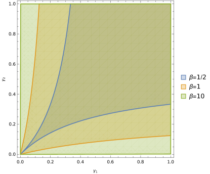
Figure 1: (color online) The “threshold condition” domain for $\beta=1/2,1,10$.

IV One mode

We start with the case of lemma 1. Let the measurement noise covariance matrix be

$$\beta=\left[\begin{array}[]{cc}\beta_{1}&0\\ 0&\beta_{2}\end{array}\right];\quad\beta_{1}\beta_{2}\geq\frac{1}{4}.$$ (45)

The corresponding complex structure is

$$J_{\beta}=\left[\begin{array}[]{cc}0&-\sqrt{\beta_{2}/\beta_{1}}\\ \sqrt{\beta_{1}/\beta_{2}}&0\end{array}\right],$$

Notice, that when $\beta_{1}=\beta_{2},$ we are in the gauge-invariant case with the standard complex structure

$$J=\left[\begin{array}[]{cc}0&-1\\ 1&0\end{array}\right].$$

The covariance matrix of the squeezed vacuum is

$$\frac{1}{2}\Delta J_{\beta}=\frac{1}{2}\left[\begin{array}[]{cc}\sqrt{\beta_{1}/\beta_{2}}&0\\ 0&\sqrt{\beta_{2}/\beta_{1}}\end{array}\right].$$

and

$$\beta+\frac{1}{2}\Delta J_{\beta}=\left[\begin{array}[]{cc}\beta_{1}+\frac{1}{2}\sqrt{\beta_{1}/\beta_{2}}&0\\ 0&\beta_{2}+\frac{1}{2}\sqrt{\beta_{2}/\beta_{1}}\end{array}\right],$$

so that $\det\left(\beta+\frac{1}{2}\Delta J_{\beta}\right)=\left(\sqrt{\beta_{1}\beta_{2}}+1/2\right)^{2},$ hence the second term in the information quantity (1) is $-\log\left(\sqrt{\beta_{1}\beta_{2}}+1/2\right).$

Let us restrict to the diagonal input covariance matrices

$$\alpha=\left[\begin{array}[]{cc}\alpha_{1}&0\\ 0&\alpha_{2}\end{array}\right],\quad\quad\alpha_{1}\alpha_{2}\geq\frac{1}{4}.$$

Then the condition (16) amounts to $\alpha_{1}\geq\frac{1}{2}\sqrt{\beta_{1}/\beta_{2}},\quad\alpha_{2}\geq\frac{1}{2}\sqrt{\beta_{2}/\beta_{1}},$ or

$$\frac{1}{4\alpha_{2}^{2}}\leq\frac{\beta_{1}}{\beta_{2}}\leq 4\alpha_{1}^{2}.$$ (46)

The matrix

$$\alpha+\beta=\left[\begin{array}[]{cc}\beta_{1}+\alpha_{1}&0\\ 0&\beta_{2}+\alpha_{2}\end{array}\right]$$

has the determinant $\left(\beta_{1}+\alpha_{1}\right)\left(\beta_{2}+\alpha_{2}\right),$ so that the information quantity (1) (and the lower bound in (III)) is

$$\max_{\mathcal{E}:\bar{\rho}_{\mathcal{E}}=\rho_{\alpha}}I(\mathcal{E},\tilde{M})=\frac{1}{2}\log\frac{\left(\beta_{1}+\alpha_{1}\right)\left(\beta_{2}+\alpha_{2}\right)}{\left(\sqrt{\beta_{1}\beta_{2}}+1/2\right)^{2}}.$$ (47)

Let us now turn to the theorem 2 for a Gaussian ensemble $\mathcal{E}=\left\{\pi_{\gamma}(d^{2}z),\rho_{\beta,z}\right\}$ with the diagonal covariance matrices

$$\gamma=\left[\begin{array}[]{cc}\gamma_{1}&0\\ 0&\gamma_{2}\end{array}\right]\geq 0$$

and $\beta$ of the form (45). By (27)

$$\tilde{\alpha}_{1}=\beta_{1}+\gamma_{1},\quad\tilde{\alpha}_{2}=\beta_{2}+\gamma_{2}.$$ (48)

Let us find the matrix

$$\tilde{\beta}=\left[\begin{array}[]{cc}\tilde{\beta}_{1}&0\\ 0&\tilde{\beta}_{2}\end{array}\right].$$

According to (28) we have

$$\tilde{\beta}_{1} = \frac{\left(\beta_{1}+\gamma_{1}\right)}{\gamma_{1}}\left[\beta_{1}-\frac{1}{4\left(\beta_{2}+\gamma_{2}\right)}\right],$$

$$\tilde{\beta}_{2} = \frac{\left(\beta_{2}+\gamma_{2}\right)}{\gamma_{2}}\left[\beta_{2}-\frac{1}{4\left(\beta_{1}+\gamma_{1}\right)}\right].$$ (49)

Note that $\beta_{1}\beta_{2}\geq 1/4$ implies $\tilde{\beta}_{1}\tilde{\beta}_{2}\geq 1/4$ as required for the covariance matrix of a Gaussian state. By (46) the condition (30) amounts to

$$\frac{1}{4\tilde{\alpha}_{2}^{2}}\leq\frac{\tilde{\beta}_{1}}{\tilde{\beta}_{2}}\leq 4\tilde{\alpha}_{1}^{2}.$$ (50)

The accessible information (26) is

$$A(\mathcal{E})=\frac{1}{2}\log\frac{\left(\tilde{\alpha}_{1}+\tilde{\beta}_{1}\right)\left(\tilde{\alpha}_{2}+\tilde{\beta}_{2}\right)}{\left(\sqrt{\tilde{\beta}_{1}\tilde{\beta}_{2}}+1/2\right)^{2}}.$$ (51)

To obtain the expressions in terms of the ensemble parameters $\gamma,\beta,$ one must substitute the relations (48), (49) into (50), (51). After some calculations which are done in the Appendix 2 we obtain the threshold condition

$$\frac{1}{4\left(\beta_{2}+\gamma_{2}\right)\beta_{2}}\leq\frac{\gamma_{1}}{\gamma_{2}}\leq 4\left(\beta_{1}+\gamma_{1}\right)\beta_{1}$$ (52)

and the accessible information

$$A(\mathcal{E})=\log\frac{\left[\left(\beta_{1}+\gamma_{1}\right)\left(\beta_{2}+\gamma_{2}\right)-\frac{1}{4}\right]}{\sqrt{\left[\left(\beta_{1}+\gamma_{1}\right)\beta_{2}-\frac{1}{4}\right]\left[\left(\beta_{2}+\gamma_{2}\right)\beta_{1}-\frac{1}{4}\right]}+\frac{\sqrt{\gamma_{1}\gamma_{2}}}{2}}.$$ (53)

Computation of the parameters (32) of the optimal Gaussian observable (31) gives

$$\beta_{\ast 1} = \frac{1}{2}\sqrt{\frac{\tilde{\beta}_{1}}{\tilde{\beta}_{2}}}\frac{\tilde{\alpha}_{1}}{\tilde{\alpha}_{2}}\left(\frac{\tilde{\alpha}_{2}-\frac{1}{2}\sqrt{\tilde{\beta}_{2}/\tilde{\beta}_{1}}}{\tilde{\alpha}_{1}-\frac{1}{2}\sqrt{\tilde{\beta}_{1}/\tilde{\beta}_{2}}}\right),$$

$$\beta_{\ast 2} = \frac{1}{2}\sqrt{\frac{\tilde{\beta}_{2}}{\tilde{\beta}_{1}}}\frac{\tilde{\alpha}_{2}}{\tilde{\alpha}_{1}}\left(\frac{\tilde{\alpha}_{1}-\frac{1}{2}\sqrt{\tilde{\beta}_{1}/\tilde{\beta}_{2}}}{\tilde{\alpha}_{2}-\frac{1}{2}\sqrt{\tilde{\beta}_{2}/\tilde{\beta}_{1}}}\right).$$

Notice that $\beta_{\ast 1}\beta_{\ast 2}=1/4$ as it must be for a squeezed vacuum.

To simplify visualization of the condition (50) we can assume without loss of generality (via a symplectic coordinate transformation) that $\beta_{1}=\beta_{2}=\beta\geq 1/2$. Then the sets of solutions $\left(\gamma_{1},\gamma_{2}\right)$ of the system (50) for $\beta=1/2,1,10,$ are shown on Fig. 1   note .

The inequality (44) becomes

$$\frac{1}{2}\log\frac{\left(\beta+\gamma_{1}+1/2\right)\left(\beta+\gamma_{2}+1/2\right)}{\left(\beta+1/2\right)^{2}}$$

$$\leq\frac{1}{2}\log\frac{\left(\beta+\gamma_{1}+\tilde{\beta}_{1}\right)\left(\beta+\gamma_{2}+\tilde{\beta}_{2}\right)}{\left(\sqrt{\tilde{\beta}_{1}\tilde{\beta}_{2}}+1/2\right)^{2}},$$

which turns into equality iff $\gamma_{1}=\gamma_{2}$ (the gauge-invariant case).

Examples of ensemble not satisfying the key condition (30) of theorem 2 are obtained by taking the parameters $\beta\geq 1/2,\gamma_{1}\geq 0,\gamma_{2}\geq 0,$ not satisfying at least one of the inequalities (52) (outer domains of curved angles on Fig. 1).  A notable case is $\gamma_{1}>0,\gamma_{2}=0,$ which corresponds to the ensemble with the Gaussian distribution $\pi_{\gamma_{1}}(dx)$ concentrated on the horizontal axis $x,$ and the family of states

$$\rho_{\beta,x}=D(x,0)\rho_{\beta}D(x,0)^{\ast},$$

where $D(x,0)=\exp(-ixp)$ are the position displacement operators and $\rho_{\beta}$ is the gauge-invariant Gaussian (thermal) state. Theorem 2 does not apply in this case while a natural conjecture is that the optimal measurement for the accessible information of this ensemble is still “Gaussian” (namely, the sharp position measurement, cf. sec. 5 of the paper entropy ).

Appendix 1

In our notations the statement of Lemma 5 of the paper  lami reads

$$\mathrm{Tr}\,W(z_{1})\sqrt{\rho_{\alpha}}W(-z_{2})\sqrt{\rho_{\alpha}}=\exp\left(-\frac{1}{2}z_{2}^{t}\alpha z_{2}-\frac{1}{2}z_{1}^{t}\alpha z_{1}+z_{2}^{t}\kappa z_{1}\right),$$ (54)

where

$$\kappa=\sqrt{I_{2s}+\left(2\alpha\Delta^{-1}\right)^{-2}}\,\alpha=\alpha\sqrt{I_{2s}+\left(2\Delta^{-1}\alpha\right)^{-2}}.$$ (55)

Sketch of proof. The quantum Fourier transform of $\sqrt{\rho_{\alpha}}$ computed in  tmf is

$$f(w) = \mathrm{Tr}\,\sqrt{\rho_{\alpha}}W(w)$$

$$= \sqrt[4]{\det\left(2\hat{\alpha}\right)}\exp\left(-\frac{1}{2}w^{t}\hat{\alpha}w\right),$$

where

$$\hat{\alpha}=\alpha+\kappa=\alpha\left(I_{2s}+\sqrt{I_{2s}+\left(2\Delta^{-1}\alpha\right)^{-2}}\right).$$

Hence

$$\mathrm{Tr}\,(W(z_{1})\sqrt{\rho_{\alpha}})\,W(w)=\mathrm{Tr}\,\sqrt{\rho_{\alpha}}W(w)W(z_{1})=\exp\left(-\frac{i}{2}w^{t}\Delta z_{1}\right)f(w+z_{1}).$$

By using Parceval relation for the quantum Fourier transform  aspekty , we have

$$\mathrm{Tr}\,W(z_{1})\sqrt{\rho_{\alpha}}W(-z_{2})\sqrt{\rho_{\alpha}}$$

$$= \mathrm{Tr}\,\left(W(z_{1})\sqrt{\rho_{\alpha}}\right)\left(\sqrt{\rho_{\alpha}}W(z_{2})\right)^{\ast}$$

$$= \frac{1}{\left(2\pi\right)^{s}}\int\exp\left(-\frac{i}{2}w^{t}\Delta z_{1}\right)f(w+z_{1})\overline{\exp\left(\frac{i}{2}w^{t}\Delta z_{2}\right)f(w+z_{2})}d^{2s}w$$

$$= \frac{1}{\left(2\pi\right)^{s}}\int\exp\left[-\frac{i}{2}w^{t}\Delta\left(z_{1}+z_{2}\right)\right]f(w+z_{1})\overline{f(w+z_{2})}d^{2s}w.$$

Substituting (Appendix 1), computing a Gaussian integral and using the relation

$$\hat{\alpha}-\frac{1}{4}\Delta\hat{\alpha}^{-1}\Delta=2\alpha$$

from the paper  scu gives (54). $\square$

Corollary 4.

The following relation holds

$$\mathrm{Tr}\,(\sqrt{\rho_{\alpha}}\rho_{\beta,z}\sqrt{\rho_{\alpha}})W(z_{1})=c\,\exp\left(iz_{1}^{t}Kz-\frac{1}{2}z_{1}^{t}\alpha_{121}z_{1}\right),$$ (57)

where

$$c=\left(\det\left(\alpha+\beta\right)\right)^{-1/2}\exp\left(-\frac{1}{2}z^{t}\left(\alpha+\beta\right)^{-1}z\right),$$

$$\alpha_{121} = \alpha-\kappa\left(\alpha+\beta\right)^{-1}\kappa,\quad$$

$$K = \kappa\left(\alpha+\beta\right)^{-1}.$$

We mention in passing that the characteristic function of the product of Gaussian density operators was obtained in  hsh .

Proof. By the inversion formula for the quantum Fourier transform  aspekty

$$\rho_{\beta,z}=\frac{1}{\left(2\pi\right)^{s}}\int\exp\left(iz_{2}^{t}z-\frac{1}{2}z_{2}^{t}\beta z_{2}\right)W(-z_{2})d^{2s}z_{2}.$$

Combining with (54),

$$\mathrm{Tr}\,\sqrt{\rho_{\alpha}}\rho_{\beta,z}\sqrt{\rho_{\alpha}}W(z_{1})$$

$$=\frac{1}{\left(2\pi\right)^{s}}\int\exp\left(iz_{2}^{t}z-\frac{1}{2}z_{2}^{t}\beta z_{2}\right) \exp\left(-\frac{1}{2}z_{2}^{t}\alpha z_{2}-\frac{1}{2}z_{1}^{t}\alpha z_{1}+z_{2}^{t}\kappa z_{1}\right)d^{2s}z_{2}.$$

Computation of the Gaussian integral results in (57). $\square$

Replacing in (57), (55) $\alpha,\beta$ by $\tilde{\alpha},\tilde{\beta}$, we rederive (40). Replacing additionally $z$ by $\tilde{K}z,$ where

$$\tilde{K}=\left(\tilde{\alpha}+\tilde{\beta}\right)\tilde{\kappa}^{-1}=\left(\tilde{\alpha}+\tilde{\beta}\right)\tilde{\alpha}^{-1}\tilde{\Upsilon}^{-1}\,$$ (58)

after some routine calculations using (41) we obtain

$$\mathrm{Tr}\,(\sqrt{\rho_{\tilde{\alpha}}}\rho_{\tilde{\beta},\tilde{K}z}\sqrt{\rho_{\tilde{\alpha}}})W(z_{1})=\frac{1}{\left|\det\tilde{K}\,\right|\sqrt{\det\gamma}}\,\exp\left(-\frac{1}{2}z^{t}\gamma^{-1}z\right)\mathrm{Tr}\,\rho_{\beta,z}W(z_{1}),$$

implying (39).

Appendix 2

Proof of (52), (53). The second inequality in (50) is the same as $\tilde{\beta}_{1}\leq 4\tilde{\alpha}_{1}^{2}\tilde{\beta}_{2}.$ By using (48), (49), we obtain

$$\tilde{\alpha}_{1}-\frac{1}{4\tilde{\alpha}_{2}}-\gamma_{1}\leq 4\tilde{\alpha}_{1}\tilde{\alpha}_{2}\frac{\gamma_{1}}{\gamma_{2}}\left(\tilde{\alpha}_{2}-\frac{1}{4\tilde{\alpha}_{1}}-\gamma_{2}\right),$$

or, introducing $D=$ $\tilde{\alpha}_{1}\tilde{\alpha}_{2}-\frac{1}{4},$

$$\frac{D}{\tilde{\alpha}_{2}}-\gamma_{1}\leq 4\tilde{\alpha}_{2}\frac{\gamma_{1}}{\gamma_{2}}D-4\tilde{\alpha}_{1}\tilde{\alpha}_{2}\gamma_{1}.$$

Rearranging and dividing by $D>0,$

$$\frac{1}{\tilde{\alpha}_{2}}\leq 4\tilde{\alpha}_{2}\frac{\gamma_{1}}{\gamma_{2}}-4\gamma_{1}=4\gamma_{1}\left(\frac{\tilde{\alpha}_{2}}{\gamma_{2}}-1\right)=4\frac{\gamma_{1}}{\gamma_{2}}\left(\tilde{\alpha}_{2}-\gamma_{2}\right),$$

which is the same as

$$\frac{1}{4\tilde{\alpha}_{2}\left(\tilde{\alpha}_{2}-\gamma_{2}\right)}\leq\frac{\gamma_{1}}{\gamma_{2}},$$

equivalent to the first inequality in (52) by (48).

Again by using (48), (49), we obtain

$$\tilde{\alpha}_{1}+\tilde{\beta}_{1}=\frac{\tilde{\alpha}_{1}}{\gamma_{1}\tilde{\alpha}_{2}}\left(\tilde{\alpha}_{1}\tilde{\alpha}_{2}-\frac{1}{4}\right),\quad\tilde{\alpha}_{2}+\tilde{\beta}_{2}=\frac{\tilde{\alpha}_{2}}{\gamma_{2}\tilde{\alpha}_{1}}\left(\tilde{\alpha}_{1}\tilde{\alpha}_{2}-\frac{1}{4}\right),$$

hence

$$\left(\tilde{\alpha}_{1}+\tilde{\beta}_{1}\right)\left(\tilde{\alpha}_{2}+\tilde{\beta}_{2}\right)=\frac{1}{\gamma_{1}\gamma_{2}}\left(\tilde{\alpha}_{1}\tilde{\alpha}_{2}-\frac{1}{4}\right)^{2}.$$

Moreover,

$$\tilde{\beta}_{1}\tilde{\beta}_{2}=\frac{1}{\gamma_{1}\gamma_{2}}\left(\tilde{\alpha}_{1}\beta_{2}-\frac{1}{4}\right)\left(\tilde{\alpha}_{2}\beta_{1}-\frac{1}{4}\right).$$

Substituting into (51) we get (53).

References

• (1) T. M. Cover and J. A. Thomas, Elements of Information Theory, 2nd edition, (John Wiley & Sons: New York, 1996).
• (2) G. De Palma, D. Trevisan, V. Giovannetti and L. Ambrosio, “Gaussian optimizers for entropic inequalities in quantum information,” J. Math. Phys. 59 (8), 081101 (2018).
• (3) V. Giovannetti, A. S. Holevo and A. Mari, “Majorization and additivity for multimode bosonic Gaussian channels,” Theor. Math. Phys. 182:2, 284–293 (2015). arXiv:1405.4066.
• (4) A. S. Holevo, Probabilistic and statistical aspects of quantum theory, 2nd edition, (Edizioni Della Normale: Pisa, 2011).
• (5) A. S. Holevo, Quantum systems, channels, information: a mathematical introduction 2-nd ed., (De Gruyter: Berlin/Boston, 2019).
• (6) A. S. Holevo, “Gaussian maximizers for quantum Gaussian observables and ensembles,” IEEE Trans. Inform. Theory 66:9, 5634-5641 (2020).
• (7) A. S. Holevo, “On the classical capacity of general quantum Gaussian measurement,” Entropy 23:3, 377 (2021).
• (8) A. S. Holevo and A. A. Kuznetsova, “Information capacity of continuous variable measurement channel,” J. Phys. A: Math. Theor. 53, 175304 (2020).
• (9) A. S. Holevo, M. Sohma and O. Hirota, “Error exponents for quantum channels with constrained inputs,” Rep. Math. Phys. 46, 343-358 (2000).
• (10) A. S. Kholevo, “On quasiequivalence of locally normal states,” Theor. Math. Phys. 13:2, 1071-1082 (1972).
https://doi.org/10.1007/BF01035528.
• (11) L. Lami, S. Das and M. M. Wilde, “Approximate reversal of quantum Gaussian dynamics,” J. Phys. A 51:12, 125301, (2018).
• (12) Gh-S. Paraoanu and H. Scutaru, “Fidelity for Multimode Thermal Squeezed States,” Phys Rev. A 61, 022306 (2000).
• (13) A. Serafini, Quantum Continuous Variables: A Primer of Theoretical Methods (CRC Press, Taylor & Francis Group, 2017).
• (14) In the previous version of the paper published in J. Math. Phys. vol.62, 092201 (2021), the domain for $\beta=1$ was shown incorrectly basing on a wrong conclusion from the present Eq. (50).