Local Critic Training for Model-Parallel Learning
of Deep Neural Networks

Abstract

In this paper, we propose a novel model-parallel learning method, called local critic training, which trains neural networks using additional modules called local critic networks. The main network is divided into several layer groups and each layer group is updated through error gradients estimated by the corresponding local critic network. We show that the proposed approach successfully decouples the update process of the layer groups for both convolutional neural networks (CNNs) and recurrent neural networks (RNNs). In addition, we demonstrate that the proposed method is guaranteed to converge to a critical point. We also show that trained networks by the proposed method can be used for structural optimization. Experimental results show that our method achieves satisfactory performance, reduces training time greatly, and decreases memory consumption per machine. Code is available at https://github.com/hjdw2/Local-critic-training.

I Introduction

Recently, deep learning has been successfully applied in many fields, including speech recognition [2],[3], machine translation [4], [5], image recognition [6], [7], etc. This achievement is mainly due to the development of large-sized neural network architectures having increased learning capabilities and the advancement of devices that can handle the huge amount of calculation for training such neural networks.

However, as the size of neural networks grows, the amounts of computation and memory consumption that a machine needs to handle increase significantly, which often becomes infeasible. A potential way to alleviate this issue is model-parallel learning by exploiting multiple computing nodes simultaneously. In this approach, a deep neural network is divided into several modules and then each module is distributed to a different computing node for efficient computation. However, the backpropagation training method that is commonly used is not suitable for this type of learning due to its sequential nature: The given data have to be processed through the entire network in the feedforward direction, producing an output. Then, the output is compared to the target using a loss function to produce an error signal. The error signal is propagated in the backward direction from the output layer to the former layers to obtain the error gradient by the chain rule, based on which the weight parameters of the network are updated. This sequential procedure ties the whole computation process into a non-breakable unit. Therefore, the distributed modules in model-parallel learning cannot be trained in an efficient way using the conventional backpropagation approach.

A few methods have been proposed for model-parallel learning. The method of auxiliary coordinates (MAC) in [8] and the alternating direction method of multipliers (ADMM) in [9] train a network by a sequence of minimization sub-steps without gradient descent steps. These methods resolve the layer-wise dependency to some extent. However, because they were only applied to shallow fully-connected networks, it is difficult to expect that the methods work well for deep network structures such as convolutional neural networks (CNNs). In [10], a concept of predicting error gradients of layers is proposed, called the decoupled neural interface (DNI) method. Prediction (instead of computation) of error gradients allows training of a certain layer before the complete backward pass till the layer. However, this method achieves poor performance when compared to conventional backpropagation as shown in [11]. Besides, when the network becomes deeper, there are cases where learning does not converge [12].

In this paper, we propose a novel method to train neural networks in a model-parallel way by introducing auxiliary neural networks, called local critic networks, to unlock dependencies in the update process of layers. We call our method local critic training. The main network is divided into several modules by the local critic networks and each local critic network delivers an estimated error gradient to the corresponding module. In this way, each module has no dependency on the other modules except the corresponding local critic network, which enables model-parallel learning. We show that the proposed method is applicable to both convolutional neural networks (CNNs) and recurrent neural networks (RNNs). Besides, we provide a theoretical analysis to demonstrate that the local critic training method converges to a critical point under certain conditions. In addition, by taking advantage of the fact that the outputs of the local critic networks indirectly approximate the output of the main network, we show that the trained networks can be used for structural optimization.

The contribution of this paper is summarized as follows.

• We propose the local critic training method for model-parallel training of deep neural networks including both CNNs and RNNs. Experimental results demonstrate that the proposed method achieves better performance of the trained networks than [10] and faster training speed and reduced memory consumption than the conventional backpropagation training.

• We mathematically prove the convergence of the proposed method.

• We show that the proposed method naturally performs structural optimization. In other words, the main and local critic networks trained by our method can form multiple networks having different levels of complexity, among which one can choose a compact one showing good performance.

The rest of the paper is organized as follows. Section II provides a brief survey of the related work. Section III explains the algorithm and architecture of the proposed local critic training method. Section IV elaborates the convergence analysis. Extensive experimental results are provided in Section V. Finally, conclusion is given in Section VI.

II Related Work

II-A Efficient Learning

In order to alleviate the burden of training huge neural networks, plenty of methods have been studied from various perspectives, such as quantization [13], pruning [14], knowledge distillation [15], hyperparameter optimization [16, 17], parallel learning [18], etc. Quantization is an approach using reduced precision floating-point numbers for weights, activations, and gradients. In [13], a method using half-precision floating point numbers is proposed, which reduces memory usage by half without performance degradation. Pruning is a method that removes weight parameters gradually during training to reduce the network size. In [14], it is shown that the proposed structured pruning and reconfiguration method reduces the training time greatly. Knowledge distillation is an approach using a pre-trained teacher network for training a student network having reduced complexity. In [15], using knowledge transfer with knowledge distillation, faster optimization and improved performance are achieved. Hyperparameter optimization is a method to find the optimal hyperparameters for learning efficiently than brute-force methods. There exist heuristic approaches using reinforcement learning to find the optimal hyperparameters during training and make the learning converge faster [16, 17]. Parallel learning uses multiple computing machines at the same time to reduce training time, which is surveyed in the following section in more detail.

II-B Parallel Learning

Parallel learning is categorized into two types: data parallelism and model parallelism.

Data parallelism basically replicates the same model on multiple machines and partitions the training dataset. Then, each machine is fed with the partitioned data to perform the forward and backward passes. The calculated error gradients are gathered at the center node to update the model parameters using stochastic gradient descent (SGD). Thus, the center node has to wait for all nodes to send the results before updating the model, which is called synchronous SGD [19]. We have another choice, in which the center node does not wait for all nodes and uses only the information available at the time, which is asynchronous SGD [20]. Some examples of recent studies on data parallelism are as follows. A method of using minimal tensor swapping between CPU and GPU is proposed in [21] to train large models beyond the GPU capacity. In [22], the effects of increasing the batch size during training for data parallelism are extensively investigated. In [18], various types of concurrency for parallelism are analyzed in the viewpoints of stochastic optimization, network architecture, and communication mechanism.

In the model parallelism approach, the model is divided into several modules and each module is trained on a different machine. This approach can speed up learning while reducing the computation burden per machine.

As a way of dividing a network, we can divide the network in terms of the arithmetic operations of layers, such as addition or multiplication. In [23], a framework for large-scale distributed training is proposed, which divides the computation process of a CNN into multiple machines, combining the asynchronous SGD. Since then, various methods have been studied to partition a network with respect to batch dimension, data dimension, or channel dimension [24, 25, 26, 27]. In addition, pipeline-based model parallel methods are proposed in [28, 29]. In [30], a method to automatically optimize parallelization strategies is proposed. A hybrid approach is also proposed in [31], where multiple devices are used for different parts of the model in each data-parallel worker. These methods, like the data parallelism methods, are usually independent of the network structure and learning algorithm. Thus, they can be used together with other model-parallel learning methods (including the proposed method) described below.

The proposed method belongs to the approach that partitions the network in the layer dimension. In [8, 9], the methods to train a network by solving an equality-constrained optimization problem are proposed, namely, MAC and ADMM, respectively. Because they do not need the gradient descesnt steps, they remove the dependencies in the update process of layers. However, these methods have proven to work only for simple networks. In [10], the method using additional neural networks called decoupled neural interfaces (DNIs) is proposed. The outputs of DNIs are the estimated error gradients of the layers in the main network for the update of the layers. Since the error gradients are provided from the DNIs, the backward pass does not need to start from the loss function. Thus, each layer can be updated independently in a layer-wise fashion. However, this method causes performance degradation compared to the backpropagation as shown in [11]. The idea of employing DNIs is also adopted in [11], where the DNIs approximate the output of the main network instead the error gradients of the layers. However, it aims to improve the performance of the model, and does not implement parallel learning. Furthermore, the methods in [10, 11] have been applied only to CNNs. In contrast, we propose a method that improves these methods to enhance the performance and also facilitate model-parallel learning for both CNNs and RNNs.

II-C Structural Optimization and Anytime Prediction

Structural optimization refers to the process of finding the optimal neural network structure to perform a given task, which has been one of the most challenging problems in neural networks [32, 33, 34, 35]. Here, the optimality can be noted as either the least complex structure achieving the maximum possible performance or the structure having a good balance between the model complexity and performance. The anytime prediction property means that given a certain computational budget that is not sufficient to perform a complete feedforward propagation through the trained network, an inference result can be still obtained using part of the network [36, 37]. CNNs and RNNs trained using the proposed local critic training algorithm are readily used for structural optimization and anytime prediction without any further training or optimization process.

III Proposed Approach

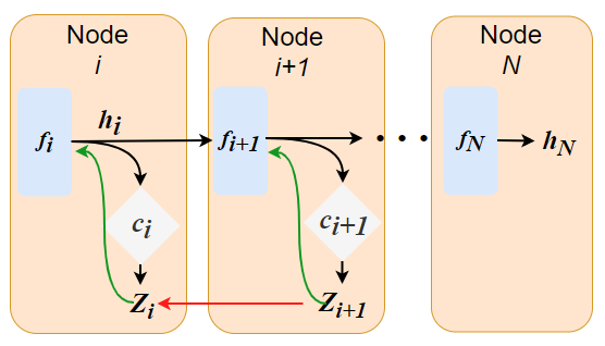
(a) CNN

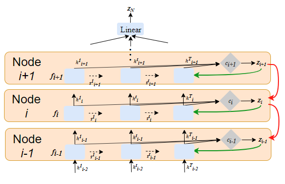
(b) RNN

Figure 1: Illustration of the proposed local critic training method. The black, green, and red arrows indicate feedforward passes, error gradient flows, and loss comparisons, respectively. Each orange box corresponds to a part that can be allocated to a separate computing node.

III-A Local Critic Training for CNNs

The core idea of the proposed local critic training method is to train the main network using additional networks called local critic networks. The local critic networks are added between layers in the main network so that the main network is divided into several layer groups, and produce outputs through softmax layers in the same manner as the output of the main network. Each local critic network is trained in such a way that the loss of its output approximates the loss of the output of the main network. Then, the corresponding layer group can be trained using the output of the local critic network without the necessity of waiting for the main network to produce the output at its final layer through the complete feedforward computation.

When the main network is divided into $N$ layer groups, we denote the $i$th layer group as $f_{i}$ ($i=1,...,N$) in the main network and the $i$th local critic network inserted between $f_{i}$ and $f_{i+1}$ as $c_{i}$ ($i=1,...,N-1$), as shown in Figure 1a. The output of $f_{i}$, denoted as $h_{i}$, is propagated to $c_{i}$, producing output $Z_{i}$. This output is compared to the target $y$ through a loss function, i.e.,

$$L_{i}=l(Z_{i},y),$$ (1)

where $l$ is the loss function such as cross-entropy or mean-squared error. Then, the error gradient for training $f_{i}$ is obtained by differentiating $L_{i}$ with respect to $h_{i}$, i.e.,

$$\delta_{i}=\frac{\partial L_{i}}{\partial h_{i}},$$ (2)

which can be used to update the weight parameters of $f_{i}$, denoted by $w_{i}$, via the gradient-descent rule:

$$w_{i}\leftarrow w_{i}-\alpha\nabla_{w_{i}}L_{i}=w_{i}-\alpha~{}\delta_{i}~{}\frac{\partial h_{i}}{\partial w_{i}},$$ (3)

where $\alpha$ is a learning rate and $\nabla_{w_{i}}$ denotes the partial derivative with respect to $w_{i}$. In order to train the weight of the layer group correctly in this way, $L_{i}$ has to appoximate the final output of the main network $L_{N}=l(h_{N},y)$ so that $\delta_{i}$ approximates the true gradient, i.e.,

$$\delta_{i}\approx\frac{\partial L_{N}}{\partial h_{i}}.$$ (4)

Thus, we can set the objective function to train $c_{i}$ as $l(L_{i},L_{N})$, which enforces $L_{i}\approx L_{N}$. However, this prevents $c_{i}$ from being updated until $L_{N}$ is obtained at the output layer of the main network. In order to alleviate such a constraint, we employ a cascaded training approach by setting the training loss for $c_{i}$ as

$$L_{c_{i}}=l(L_{i},L_{i+1}).$$ (5)

As a result, as learning progresses, $L_{i}$ can eventually approximate $L_{N}$. Thus, each local critic network can be also updated to optimize the loss function given in (5) once the approximated loss by the subsequent layer, $L_{i+1}$, is available.

Therefore, the loss approximation by the local critic networks and the cascaded training of the local critic networks effectively alleviate the dependencies between layers in both the forward and backward passes. All layers in the network are dependent only on adjacent layers so that we can train the entire network in a model-parallel way by distributing the layer groups to different computing nodes as shown in Figure 1a.

III-B Local Critic Training for RNNs

Figure 1b illustrates the architecture and training process of the proposed method for RNNs. The $i$th layer group in the main RNN, denoted as $f_{i}$ ($i=1,...,N$) receives the output of the previous layer group, $h_{i-1}^{t}$, where $t=1,...,T$ indicates the time index, and produces its output, $h_{i}^{t}$. The final network output $Z_{N}=[z_{N}^{1},z_{N}^{2},...,z_{N}^{T}]^{\top}$ is obtained by aggregating the $N$th layer group’s outputs over time (i.e., $h_{N}^{t}$) through a linear layer, where $\top$ is the transpose operation.

As in the case of CNNs, we introduce an additional local critic network $c_{i}$ ($i=1,...,N-1$) attached to the $i$th layer group. It takes all the outputs of the layer group (i.e., $h_{i}^{t}$, $t=1,...,T$) as input and produces the output $Z_{i}=[z_{i}^{1},z_{i}^{2},...,z_{i}^{T}]^{\top}$ that has the same dimension to the output of the main network $Z_{N}$. Then, with $L_{i}^{t}=l(z_{i}^{t},y^{t})$, the loss $L_{i}$ of $c_{i}$ is obtained by

$$L_{i}=\sum_{t=1}^{T}{L_{i}^{t}},$$ (6)

which in turn allows approximation of the error gradient:

$$\delta_{i}=\left[\frac{\partial L_{i}^{1}}{\partial h_{i}^{1}},\frac{\partial L_{i}^{2}}{\partial h_{i}^{2}},...,\frac{\partial L_{i}^{T}}{\partial h_{i}^{T}}\right]^{\top}\approx\left[\frac{\partial L_{N}^{1}}{\partial h_{N}^{1}},\frac{\partial L_{N}^{2}}{\partial h_{N}^{2}},...,\frac{\partial L_{N}^{T}}{\partial h_{N}^{T}}\right]^{\top}.$$ (7)

Then, the gradient descent rule is used to update the weight parameters of $f_{i}$, denoted as $w_{i}$:

$$w_{i}\leftarrow w_{i}-\alpha\nabla_{w_{i}}L_{i}=w_{i}-\alpha~{}\delta_{i}^{\top}~{}g_{i},$$ (8)

where $\alpha$ is a learning rate and $g_{i}=\left[\frac{\partial h_{i}^{1}}{\partial w_{i}},\frac{\partial h_{i}^{2}}{\partial w_{i}},...,\frac{\partial h_{i}^{T}}{\partial w_{i}}\right]^{\top}$. In order to train the network in a model-parallel way, we use the loss function in (5) to train the local critic networks. Therefore, as in the case of CNNs, each layer group can be independently updated based on the corresponding local critic network without waiting for the complete feedforward and backward passes.

III-C Structure Optimization and Anytime Prediction

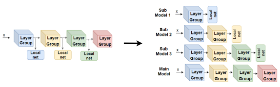
(a) CNN

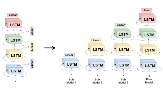
(b) RNN

Figure 2: Sub-models obtained by the proposed training approach.

Training of $c_{i}$ allows it to eventually approximate the main network’s output since it is trained to minimize the loss difference from the next local critic network $c_{i+1}$ by the objective (5). After the training finishes, thus, we have several sub-models that can perform the same task, as shown in Figure 2, each of which consists of a certain number of layers and a local critic network, i.e., $f_{1}$ through $f_{i}$ and $c_{i}$. Depending on the number of layers, each sub-model has different model complexity (in terms of the number of weight parameters and the number of floating number operations) and possibly different performance. Among them, we can choose a suitable one by considering the trade-off between the complexity and the performance, accomplishing structural optimization for the given task.

This is also equivalent to implementing a simple anytime prediction mechanism. In other words, if the given computational budget is small, a shallow sub-model can be used for producing output, whereas if the budget is sufficient, an output can be obtained using a deeper sub-model or even the main network, which is more reliable in general. Our approach is beneficial in that generic CNNs and RNNs can be made to perform anytime prediction, whereas previous approaches (e.g., [36, 37]) rely on special network structures.

IV Convergence Analysis

This section provides a theoretical analysis for convergence of the proposed local critic training algorithm. By exploiting the analysis in [38], we prove that the algorithm is guaranteed to converge to a critical point.

Since we use the SGD method, the weight parameters of each layer group in the main network are updated according to (3), i.e.,

$$w_{i}^{k+1} =w_{i}^{k}-\alpha_{k}\nabla_{w_{i}}L_{i}(w_{1:i}^{k},\xi_{k}),$$ (9)

where $w_{i}^{k}$ is the weight parameters of the $i$th layer group at the $k$th training iteration ($k=1,...,K$), $w_{1:i}^{k}$ is the collection of the weight parameters in the first to $i$th layer groups at the $k$th training iteration, and $\xi_{k}$ is the random variable for a set of samples in the mini-batch SGD method. Thus, we have the following update rule for all the weight parameters of the main network:

$$w_{1:N}^{k+1} =w_{1:N}^{k}-\alpha_{k}\nabla_{w}L(w^{k},\xi_{k}),$$ (10)

where

$$\nabla_{w}L(w^{k},\xi_{k})=\begin{bmatrix}\nabla_{w_{1}}L_{1}(w_{1}^{k},\xi_{k})\\ \vdots\\ \nabla_{w_{N}}L_{N}(w_{1:N}^{k},\xi_{k})\\ \end{bmatrix}.$$ (11)

First, as in [12], we build a connection between the true gradient and the stochastic gradients from the local critic networks in Assumption 1.

Assumption 1 It is assumed that $w_{1:N}$ is updated in a descending direction of the true loss by the local critic training method. For this, the estimated stochastic gradient direction from the local critic networks, $\nabla_{w}L(w^{k},\xi_{k})$, is assumed to be a sufficient descent direction of the true loss, $\nabla L_{N}$. In other words, there exists a constant $\sigma>0$ such that

$$\nabla L_{N}(w_{1:N}^{k})^{\top}\nabla_{w}L(w^{k},\xi_{k})\geq\sigma\left\|\nabla L_{N}(w_{1:N}^{k})\right\|_{2}^{2}.$$ (12)

This means that when each layer group is trained by the gradient from the loss function of the corresponding local critic network, the learning direction is similar to the direction of the gradient from the loss function of the main network. We demonstrate the validity of this assumption in Section V-A through experiments.

Next, we assume that the second moment of the stochastic gradient descent is upper bounded to restict the variance of the stochastic gradient descent.

Assumption 2 It is assumed that there exists a constant $M\geq 0$ such that

$${}_{\xi_{k}}\left[\left\|\nabla_{w}L(w^{k},\xi_{k})\right\|_{2}^{2}\right]\leq M.$$ (13)

In other words, the magnitude of the estimated gradient is bounded and does not diverge. This is valid when the weights are in a bounded set, which would hold in general.

Finally, we assume smoothness of the objective function, i.e., the gradient of the objective function does not change arbitrarily quickly with respect to the weight parameters.

Assumption 3 It is assumed that the objective function $L_{N}$ is continuously differentiable and the gradient of $L_{N}$ is Lipschitz continuous with Lipschitz constant $\lambda>0$, i.e.,

$$\left\|\nabla L_{N}(w_{1:N})-\nabla L_{N}(w_{1:N}^{\prime})\right\|_{2}\;\leq\lambda\left\|w_{1:N}-w_{1:N}^{\prime}\right\|_{2}.$$ (14)

The following theorem shows that the proposed method converges to a critical point.

Theorem 1 Suppose that the local critic training method is run with a learning rate sequence satisfying $\sum\limits_{k=0}^{\infty}\alpha_{k}=\infty$ and $\sum\limits_{k=0}^{\infty}\alpha_{k}^{2}<\infty$. Under Assumptions 1, 2, and 3, and if we further assume that the objective function $L_{N}$ is twice differentiable, and the mapping $w_{1:N}\rightarrow\left\|\nabla L_{N}(w_{1:N}^{k})\right\|_{2}^{2}$ has Lipschitz continuous derivatives, then

$$\lim_{k\to\infty}\E\left[\left\|\nabla L_{N}(w_{1:N}^{k})\right\|_{2}^{2}\right]=0.$$ (15)

Since the expected squared norm of the gradient converges to zero, the proposed local critic training method converges to a critical point. The proof of the theorem is given in Appendix 1.

V Experiments

In this section, we present experimental results to examine the performance of our method in various aspects, including classification accuracy, training time, memory consumption, and structural optimization for CNNs and RNNs.

For CNNs, we evaluate the method with ResNet models [39] (ResNet-50 and ResNet-101) on three image classification benchmark datasets: CIFAR-10, CIFAR-100 [40], and ImageNet [41]. We employ the SGD with a momentum of 0.9 for the main networks and the Adam optimization with a fixed learning rate of $1\times 10^{-4}$ for the local critic networks. The L2 regularization is used with a fixed constant of $5\times 10^{-4}$ for the main networks. For the loss functions in (1) and (5), we use the cross-entropy and the L1 loss, respectively, which is determined empirically. For CIFAR-10 and CIFAR-100, the batch size is set to 128 and the maximum training iteration is set to 80,000. The learning rate for the main networks is initialized to 0.1 and dropped by an order of magnitude after 40,000 and 60,000 iterations. We use one convolutional layer with the ReLU activation function and a fully-connected layer for each local critic network. For ImageNet, the batch size is set to 32 and the maximum training epoch is set to 75. The learning rate for the main networks is initialized to 0.0125 and dropped by an order of magnitude after 23, 40, 60, and 70 epochs. We use two convolutional layers with the ReLU activation function and a 1-channel convolutional layer for each local critic network.

For RNNs, two character-level datasets, Penn Tree Bank (PTB) [42] and Hutter Wikipedia Prize (enwik8) [43], are used for benchmarking with long short-term memory (LSTM) units [44]. The bits per character (BPC) is used as a measure of performance. The structures of the main network and each local critic network are a multi-layer LSTM cell and a fully-connected layer, respectively. As in the case of CNNs, the cross-entropy and the L1 loss are used for the loss functions in (6) and (5), respectively. The batch size is set to 128, the backpropagation through time (BPTT) length is set to 150, and the embedding size is set to 128 for both datasets. The L2 regularization is used with a fixed constant of $1.2\times 10^{-5}$ for the main network. For PTB, we apply the Adam optimization for 100 epochs with a learning rate that is initially set to $2.7\times 10^{-3}$ and reduced by 0.33 at every 20 epochs. For enwik8, we use the Adam optimization with a fixed learning rate of $1.0\times 10^{-4}$ for 50 epochs.

The locations of the local critic networks in the main network are determined in such a way that the number of layers in each layer group is distributed as evenly as possible for all cases. We denote the case with $n$ local critic networks by LCT_n$n$.

All experiments are performed using TensorFlow with GTX1080Ti graphics processing units (GPUs). The number of employed GPUs is equal to the number of layer groups, i.e., $N$. Each layer group and the corresponding local critic network are allocated to each GPU.

V-A Sufficient Descent Direction

To demonstrate the validity of the analysis in Section IV, we experimentally verify that Assumption 1 is satisfied. For each training epoch, we calculate the gradient from the loss function of the main network, $\nabla L_{N}(w_{1:N}^{k})$, and its squared magnitude, $\left\|\nabla L_{N}(w_{1:N}^{k})\right\|_{2}^{2}$, and the gradient from the loss function of the local critic network, $\nabla_{w}L(w^{k},\xi_{k})$, for each layer group. Since the inequality (12) can be written as

$$\frac{\nabla L_{N}(w_{1:N}^{k})^{\top}\nabla_{w}L(w^{k},\xi_{k})}{\left\|\nabla L_{N}(w_{1:N}^{k})\right\|_{2}^{2}}\geq\sigma,$$ (16)

we compute $\nabla L_{N}(w_{1:N}^{k})^{\top}\nabla_{w}L(w^{k},\xi_{k})/\left\|\nabla L_{N}(w_{1:N}^{k})\right\|_{2}^{2}$ to obtain the maximum value of $\sigma$ for each layer group and check if this value is greater than zero during training.

Figures 3 and 4 examine the obtained maximum value of $\sigma$ in each layer group during training for the cases with one local critic network (LCT_n1) and three local critic networks (LCT_n3). We employ ResNet-50 for CNNs and four layers of LSTM units for RNNs. We omit the result of the last layer group in all cases since the last layer group is trained by the regular backpropagation and thus $\sigma$ is always one.

The figures confirm that $\sigma$ is larger than 0 at all times during training for all cases of CNNs and RNNs. Therefore, Assumption 1 is satisfied and the convergence analysis in Section IV is valid.

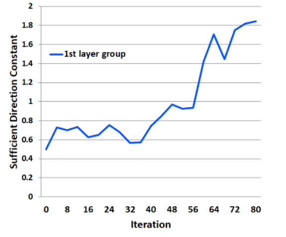
(a) LCT_n1 for CIFAR-10

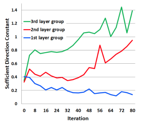
(b) LCT_n3 for CIFAR-10

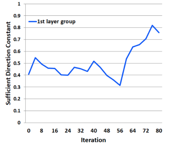
(c) LCT_n1 for CIFAR-100

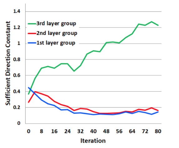
(d) LCT_n3 for CIFAR-100

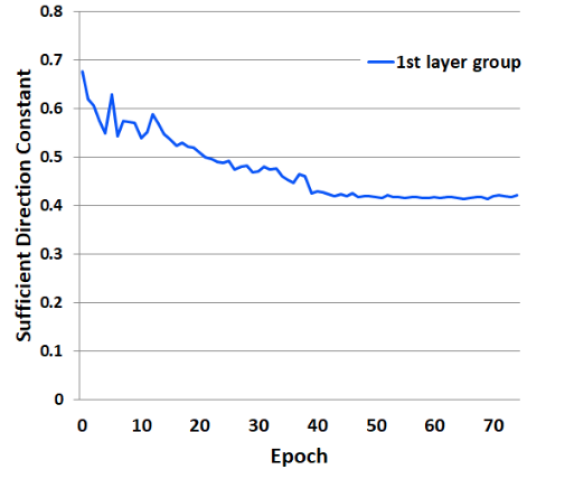
(e) LCT_n1 for ImageNet

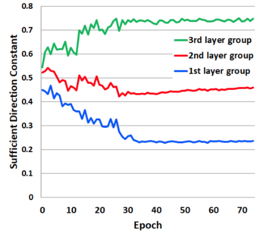
(f) LCT_n3 for ImageNet

Figure 3: Value of constant $\sigma$ during training for ResNet-50

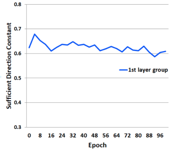
(a) LCT_n1 for PTB

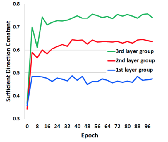
(b) LCT_n3 for PTB

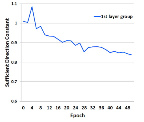
(c) LCT_n1 for enwik8

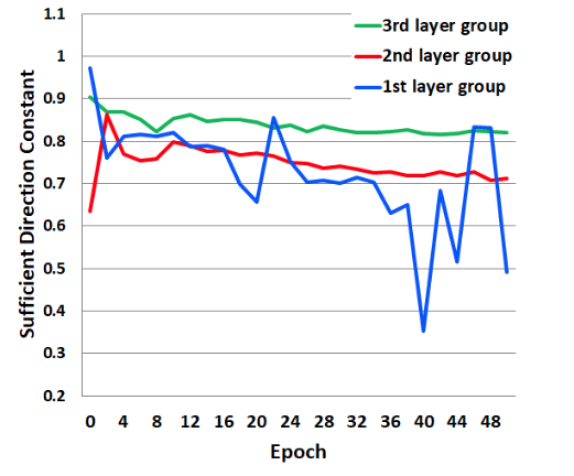
(d) LCT_n3 for enwik8

Figure 4: Value of constant $\sigma$ during training for RNNs with four layers of LSTM units

V-B Performance Evaluation

V-B1 CNN

TABLE I: Test accuracy (%) of backpropagation (BP), DNI, and the proposed local critic training method (LCT).

ResNet-50	BP	DNI_n1	DNI_n2	DNI_n3	LCT_n1	LCT_n2	LCT_n3
CIFAR-10	93.79	80.07	74.59	71.24	91.41	92.64	93.32
CIFAR-100	76.16	49.44	43.39	43.31	73.65	71.37	70.90
ImageNet Top-1 Top-5	72.09 90.51	-	-	-	67.80 88.24	67.67 88.07	65.81 86.79
ResNet-101	BP	DNI_n1	DNI_n2	DNI_n3	LCT_n1	LCT_n2	LCT_n3
CIFAR-10	93.77	75.70	66.53	65.46	93.25	93.10	93.34
CIFAR-100	76.76	43.94	35.37	33.62	71.82	72.14	72.10
ImageNet Top-1 Top-5	73.38 91.37	-	-	-	72.11 90.66	68.20 88.34	67.05 87.80

TABLE II: Test accuracy (%) of backpropagation (BP) and the proposed local critic training method (LCT) for ResNet-182.

	BP	LCT_n1	LCT_n2	LCT_n3
CIFAR-10	94.80	92.89	94.10	93.00
CIFAR-100	77.46	73.29	72.50	72.74
ImageNet Top-1 Top-5	75.42 92.33	74.13 91.63	70.62 89.82	66.46 87.43

TABLE III: Test accuracy (%) of backpropagation (BP), ADMM, DNI, and the proposed local critic training method (LCT) for a multilayer perceptron having 300, 150, and 10 units.

	BP	ADMM	DNI_n1	LCT_n1
MNIST	98.05	82.53	95.99	98.09
CIFAR-10	61.22	19.29	35.75	61.28

TABLE IV: Test accuracy (%) of backpropagation with joint losses obtained from the same network structure to LCT_n3.

	ResNet-50	ResNet-101
CIFAR-10	94.80	94.52
CIFAR-100	76.39	75.37
ImageNet Top-1 Top-5	71.86 90.32	72.40 90.66

We evaluate the classification performance of the proposed local critic training method with different numbers of local critic networks. We also compare the results of the regular backpropagation and DNI method [10] as shown in Table I. For the DNI method, the layers of the main network are grouped in the same way to our method, and each DNI is implemented with three convolutional layers, which shows the best performance in our experiment.

For CIFAR-10, the proposed method achieves comparable performance to the regular backpropagation. The performance varies with the number of local critic networks (and the number of layer groups, accordingly), but the test accuracy of the proposed method with four layer groups is almost the same to that of the backpropagation (93.79% vs. 93.32% with ResNet-50, and 93.77% vs. 93.34% with ResNet-101). When compared to the DNI method, our method achieves much better performance in all cases. For CIFAR-100, the test accuracy of our method is slightly lower when compared to that of the backpropagation. However, it is significantly higher than that of the DNI approach. Similarly, for ImageNet, the proposed method shows only slightly lowered accuracy compared to the backpropagation, whereas DNI fails to converge in all cases. These results show that our method can train the large-sized CNNs in a model-parallel way at the cost of slight accuracy drops and significantly outperform the existing DNI method.

Using more local critic networks allows us to exploit more computing nodes simultaneously for faster training (Section V-C), but intuitively, it causes larger accuracy drop because of more approximation stages. Thus, the classification accuracy and the number of local critic networks are in a tradeoff relationship, which is observed in the results for ImageNet. Such a relationship is not quite clear for CIFAR-10 and CIFAR-100, which is probably because those datasets are not significantly challenging and thus gradient estimation using local critic networks does not impose significant difficulty in training.

In order to validate that our method works for networks even larger than ResNet-101, we employ ResNet-182, which is the largest size that our single GPU machine (GTX1080Ti with 11GB memory) can afford. It has ten more 3-layer bottleneck blocks than ResNet-152 on the feature map of 28$\times$28 (i.e., conv4) [39]. Table II demonstrates that our method performs well on this large-sized network, showing similar trends to those in Table I.

In contrast, we also examine if the proposed method can achieve satisfactory performance for shallow networks compared to the existing methods including ADMM [9] and DNI. For this, we use a multilayer perceptron consisting of three dense layers having 300, 150, and 10 units, respectively, with the ReLU activation function. The results for MNIST and CIFAR-10 are shown in Table III. Unlike ADMM and DNI showing degraded performance, our method achieves almost the same performance to backpropagation.

As shown in [45], using extra layers as early exits (like our network structure) and combining the losses of the exits for backpropagation may achieve higher performance than the original network. Thus, we evaluate the performance of backpropagation using the joint losses as in [45] with the same network structure used for LCT_n3. However, the results presented in Table IV show that it is not clear whether using joint losses improves performance than the original backpropagation. For CIFAR-10, the performance of backpropagation using joint losses is slightly improved than the original backpropagation, but for CIFAR-100 and ImageNet, the performance is rather reduced. Since the structures of our local critic networks are extremely simple to reduce the computational burden, the losses of the early exits seem to have a negative effect on the whole learning for complex data.

V-B2 RNN

TABLE V: Test BPC of the backpropagation (BP) and the proposed local critic training method (LCT) with varying the number of layers in the main network. The number of LSTM units per layer is also shown in each case.

	$\#$ of layers ($\#$ of LSTM units)	2 (950)	3 (750)	4 (600)
PTB	BP LCT	1.275 1.276	1.288 1.265	1.275 1.269
enwik8	BP LCT	1.476 1.469	1.509 1.492	1.618 1.541

We evaluate the performance of the proposed local critic training method in comparison to the conventional backpropagation with respect to the number of layers in the main network. In this experiment, we deploy local critic networks between every layer pair in the main network. The number of LSTM units in each layer of the main network is determined by the memory limitation of the used GPU for backpropagation.

The results are shown in Table V. The performance of the local critic training method is similar to or, in most cases, even better than that of the backpropagation, which demonstrates that using the estimated error gradients is effective particularly for training RNNs. Therefore, we can conclude that the proposed method can unlock the layer-wise dependencies without performance degradation over a wide range of the number of RNN layers.

V-C Complexity

We evaluate the computation and memory complexities of the proposed method.

V-C1 Training Time

We compare the training time of LCT_n1, LCT_n3, and the backpropagation for CNNs and RNNs until the maximum epoch (or iteration) reaches. In Figure 5, we show the loss with respect to the training time of ResNet-50 and ResNet-101 for CIFAR-10 and CIFAR-100. In all cases, the training time of LCT_n3 is the shortest, followed by that of LCT_n1. For CIFAR-10, training time is reduced by 27.8% for LCT_n1 and 33.6% for LCT_n3 in comparison to the backpropagation with ResNet-50. With ResNet-101, the relative training time reduction is 31.9% for LCT_n1 and 40.9% for LCT_n3. For CIFAR-100, the amounts of training time reduction are 32.0% for LCT_n1 and 34.2% for LCT_n3 with ResNet-50, and 32.4% for LCT_n1 and 43.9% for LCT_n3 with ResNet-101. Figure 6 shows the BPC of LSTM networks having four layers with respect to the training time for PTB. The training time is reduced by 16.7% for LCT_n1 and 35.8% for LCT_n3 for PTB in comparison to backpropagation. These results demonstrate that the proposed method can implement efficient model-parallel training.

The training time of the proposed method includes the time for communication between different computing nodes. We investigate the relative amount of such communication time. Since it is difficult to directly measure it during training, we measure the time required for a variable of the same size with the data to be transmitted (i.e., the outputs of the layer groups for the feedforward pass and the losses from the local critic networks for the backward pass). For CIFAR-10, the time for communication is 3.79% of the total training time for LCT_n1 and 8.67% for LCT_n3 with ResNet-50, and 1.47% for LCT_n1 and 3.58% for LCT_n3 with ResNet-101. Therefore, although the communication time increases as the network is divided more, its proportion to the total learning time decreases as the network becomes larger. Overall, we can say that the communication time is relatively short or even negligible.

In addition, we compare our method with a simple pipelined version of backpropagation. In other words, after splitting the network into several layer groups that are allocated to different computing nodes, each node can concurrently run the feedforward pass by delivering the output to the next node and then immediately receiving a new input from the previous node. Thus, it is a basic model-parallel learning strategy that has no performance difference from the original backpropagation and can reduce the learning time. Note that, since this method is implemented in Pytorch, its result cannot be directly compared with the results shown above. In order to enable comparison between these results and the results of our method implemented in Tensorflow, we normalize the training time of the pipelined backpropagation with that of the original backpropagation. We compare the training time of the pipelined backpropagation using 2 GPUs and 4 GPUs, which correspond to LCT_n1 and LCT_n3, respectively. As shown in Figure 7, for CIFAR-100, the training time of our method is shorter by 15.7% for LCT_n1 and 3.5% for LCT_n3 than that of the corresponding pipeline backpropagation for ResNet-101. Therefore, our method is more effective even when compared to a pipelined version of backpropagation. Moreover, it would be also possible to combine this pipelining method into our method for further improvement of our method.

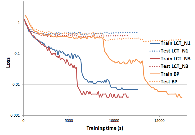
(a) ResNet-50 for CIFAR-10

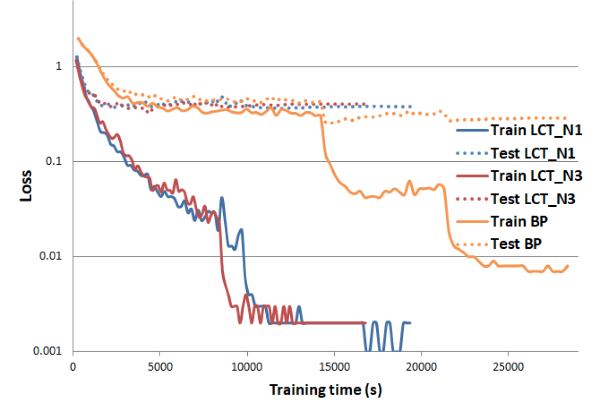
(b) ResNet-101 for CIFAR-10

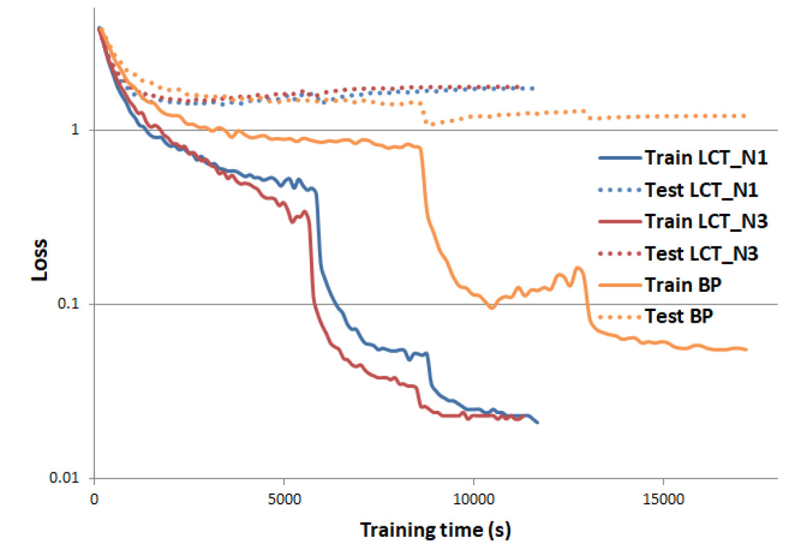
(c) ResNet-50 for CIFAR-100

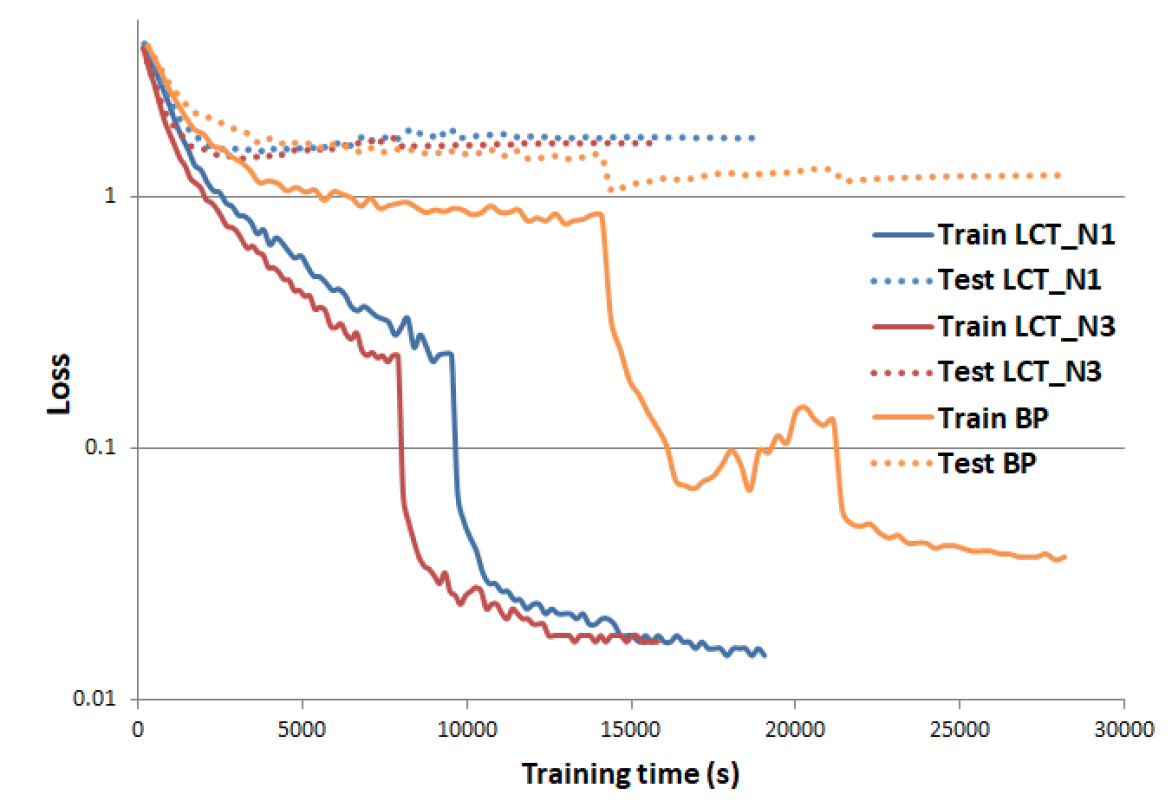
(d) ResNet-101 for CIFAR-100

Figure 5: Training and test losses with respect to the elapsed time for CNNs

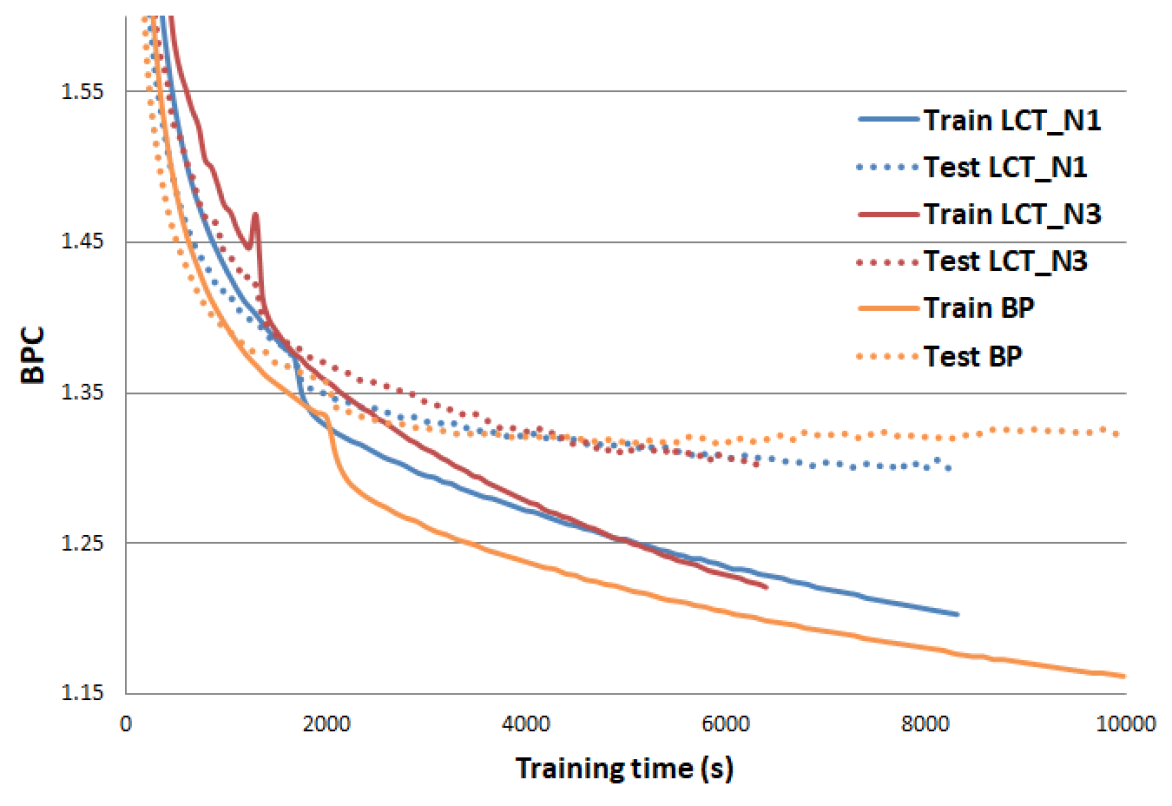
Figure 6: Training and test losses with respect to the elapsed time for the LSTM networks having four layers

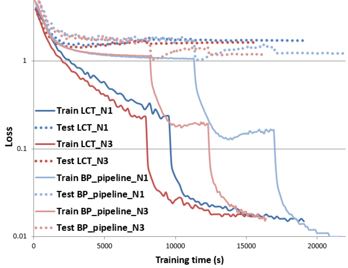
Figure 7: Training and test losses of the pipelined backpropagation and the proposed method with respect to the elapsed time with ResNet-101 for CIFAR-100

V-C2 Memory Consumption

By splitting the computation for training among multiple computing nodes, the proposed method can additionally reduce the amount of memory usage per computing node. We compare the memory consumption per GPU by our method and the backpropagation for ImageNet and PTB in Table VI. It is shown that even if the total amount of memory consumption increases, we can alleviate the burden of the memory consumption per GPU. Additionally, when compared to the DNI method for CIFAR-100, there is almost no difference between our method and the DNI method; the memory usage of our method is 4659, 5461, 5463, and 5459 MiB for each GPU, respectively, and that of DNI is 4693, 5453, 4943, and 5459 MiB for each GPU, respectively.

Note that the layer grouping and the location of the local critic networks were not determined by considering the memory usage. If the memory constraints are significant, the layer grouping can be designed in a more memory-efficient way.

TABLE VI: Memory consumption (MiB) per GPU by backpropagation (BP) and the proposed local critic training method (LCT_n3) for the ImageNet and PTB datasets.

ResNet-50 (ImageNet)	GPU 1	GPU 2	GPU 3	GPU 4
BP	8807	-	-	-
LCT_n3	3207	3077	7141	7171
ResNet-101 (ImageNet)	GPU 1	GPU 2	GPU 3	GPU 4
BP	8789	-	-	-
LCT_n3	4663	7141	5863	5127
4-layer LSTM (PTB)	GPU 1	GPU 2	GPU 3	GPU 4
BP	8695	-	-	-
LCT_n3	4573	2441	2441	4489

V-D Structural Optimization and Anytime Prediction

V-D1 CNN

As depicted in Figure 2, we obtain several trained sub-models in addition to the trained main network as a result of application of the local critic training method. Table VII shows their performance, and Table VIII analyzes their complexity in terms of computational complexity (the number of floating-point operations (FLOPs)) required for one feedforward pass and memory complexity (the number of weight parameters) for the case using three local critic networks (LCT_n3). In Table VIII, the complexity of each local critic network itself with the percentage over the total complexity of the corresponding sub-model is also shown.

As expected, the larger the network is, the higher the classification accuracy is, which is reasonable because a larger network has a greater capability of learning the data. However, the largest network (i.e., the main network) is not necessarily the optimal structure when both the accuracy and model complexity are considered. For CIFAR-10, Sub_3 of ResNet-50 and Sub_2 of ResNet-100 show almost the same accuracy to the corresponding main networks, each of which reduces the complexity by about 59% (47.55 to 19.53 million FLOPs and 23.82 to 9.79 million parameters) and 72% (85.17 to 23.99 million FLOPs and 42.68 to 12.03 million parameters), respectively. Interestingly, these sub-models have roughly similar complexities, showing that regardless of the starting network (ResNet-50 or ResNet-100), the structural optimization results could be similar. For CIFAR-100, the same result of structural optimization can be obtained with minor accuracy loss (0.93 to 1.61%). For a more challenging dataset, i.e., ImageNet, reduction of the complexities via choosing the best sub-model (i.e., Sub_3) is obtained at the cost of slight accuracy loss.

Choosing smaller sub-models results in larger accuracy loss but more significant complexity reduction. Therefore, when there exist resource limitations in a target application, the model can be chosen among the sub-models and main network by considering the trade-off between the performance and the complexity.

Anytime prediction can be implemented in a similar way. When a computational budget is given, a sub-model satisfying the budget can be chosen to produce the output. As shown in Table VII, the more budget we have, the more accurate the prediction is.

TABLE VII: Test accuracy (%) of the main model and the sub-models for CNNs (LCT_n3).

ResNet-50	Sub_1	Sub_2	Sub_3	Main
CIFAR-10	86.78	91.40	93.24	93.32
CIFAR-100	60.03	66.71	69.29	70.90
ImageNet Top-1 Top-5	36.59 62.18	49.98 75.08	60.73 83.30	65.81 86.79
ResNet-101	Sub_1	Sub_2	Sub_3	Main
CIFAR-10	91.68	93.35	93.33	93.34
CIFAR-100	67.22	71.17	71.59	72.10
ImageNet Top-1 Top-5	49.44 75.11	62.68 84.80	63.69 85.44	67.05 87.80

TABLE VIII: FLOPs required for a feedforward pass and numbers of model parameters in the sub-models and main model for CNNs (LCT_n3). The complexity of each local critic network itself with the percentage over the total complexity is shown in parentheses.

CIFAR-10 CIFAR-100 ImageNet ResNet-50 FLOP (M) $\#$ of parameters (M) FLOP (M) $\#$ of parameters (M) FLOP (M) $\#$ of parameters (M) Sub_1 3.64 (3.21, 88%) 1.82 (1.61, 88%) 27.24 (26.80, 98%) 13.62 (13.40, 98%) 0.95 (0.50, 53%) 0.47 (0.25, 53%) Sub_2 4.71 (1.84, 39%) 2.35 (0.92, 39%) 10.61 (7.73, 73%) 5.30 (3.87, 73%) 3.68 (0.79, 21%) 1.84 (0.40, 22%) Sub_3 19.61 (2.52, 13%) 9.79 (1.26, 13%) 21.08 (4.00, 19%) 10.53 (2.00, 19%) 18.48 (1.38, 7%) 9.23 (0.69, 7%) Main 47.69 23.82 53.58 26.77 51.15 25.55 ResNet-101 FLOP (M) $\#$ of parameters (M) FLOP (M) $\#$ of parameters (M) FLOP (M) $\#$ of parameters (M) Sub_1 4.71 (1.84, 39%) 2.35 (0.92, 39%) 10.61 (7.73, 73%) 5.30 (3.87, 73%) 3.68 (0.79, 21%) 1.84 (0.40, 22%) Sub_2 24.08 (2.52, 10%) 12.03 (1.26, 10%) 25.56 (4.00, 16%) 12.76 (2.00, 16%) 25.19 (1.38, 5%) 12.58 (0.69, 5%) Sub_3 44.08 (2.52, 6%) 22.01 (1.26, 6%) 45.55 (4.00, 9%) 22.75 (2.00, 9%) 47.43 (1.38, 3%) 23.68 (0.69, 3%) Main 85.44 42.68 91.34 45.62 93.38 46.64

V-D2 RNN

TABLE IX: Test BPC of the main model and the sub-models for 4-layer LSTM networks (LCT_n3).

	Sub_1	Sub_2	Sub_3	Main
PTB	1.329	1.281	1.272	1.269
enwik8	1.691	1.585	1.551	1.541

We show the performance (BPC) of the sub-models and the main model of RNNs in Table IX and their computational complexity for one feedforward pass and the number of weight parameters in Table X for the case using three local critic networks (LCT_n3). The complexity of each local critic network itself with the percentage over the total complexity of the corresponding sub-model is also shown.

As in the CNN cases, an optimal network structure can be chosen by considering the trade-off relationship between the performance and complexity. The largest sub-models (Sub_3) achieve almost the same performance to that of the main model (1.272 vs. 1.269 for PTB, and 1.551 vs. 1.541 for enwik8), while they can reduce the computational and memory complexities by about 28% (401 to 290 billion FLOPs and 10.43 to 7.55 million parameters). The performance of the smaller sub-models is slightly worse than that of the main model, but the complexity reduction is more significant (reductions by about 55% and 83% with Sub_2 and Sub_1, respectively). Anytime prediction can be also performed using the sub-models requiring lower complexities than the main model.

TABLE X: FLOPs required for a feedforward pass and the numbers of model parameters in the sub-models and main model for 4-layer LSTM networks (LCT_n3). The complexity of each local critic network itself with the percentage over the total complexity is shown in parentheses.

	FLOP (B)	$\#$ of parameters (M)
Sub_1	68 (1.15, 1.7%)	1.79 (0.03, 1.7%)
Sub_2	179 (1.15, 0.6%)	4.67 (0.03, 0.6%)
Sub_3	290 (1.15, 0.4%)	7.55 (0.03, 0.4%)
Main	401	10.43

VI Conclusion

In this paper, we proposed the local critic training method for model-parallel training of CNNs and RNNs. The mathematical analysis showed the convergence of the proposed method. Through the experiments, we confirmed the effectiveness of the method, including the satisfactory classification performance, faster training speed, and lower memory consumption per GPU. It was also shown that structural optimization and anytime prediction can be achieved using the models trained by the proposed method.

Appendix A Proof of Theorem 1

Let us begin with rewriting $L_{N}(w_{1:N}^{k+1})$ as

$$L_{N}(w_{1:N}^{k+1}) =L_{N}(w_{1:N}^{k})+\int_{0}^{1}\frac{\partial L_{N}(w_{1:N}^{k}+\tau(w_{1:N}^{k+1}-w_{1:N}^{k}))}{\partial\tau}\,d\tau$$ (17)

$$=L_{N}(w_{1:N}^{k})+\int_{0}^{1}\nabla L_{N}(w_{1:N}^{k}+\tau(w_{1:N}^{k+1}-w_{1:N}^{k}))^{\top}(w_{1:N}^{k+1}-w_{1:N}^{k})\,d\tau$$ (18)

$$=L_{N}(w_{1:N}^{k})+\nabla L_{N}(w_{1:N}^{k})^{\top}(w_{1:N}^{k+1}-w_{1:N}^{k})+\int_{0}^{1}(\nabla L_{N}(w_{1:N}^{k}+\tau(w_{1:N}^{k+1}-w_{1:N}^{k}))-\nabla L_{N}(w_{1:N}^{k}))^{\top}(w_{1:N}^{k+1}-w_{1:N}^{k})\,d\tau$$ (19)

$$\leq L_{N}(w_{1:N}^{k})+\nabla L_{N}(w_{1:N}^{k})^{\top}(w_{1:N}^{k+1}-w_{1:N}^{k})+\int_{0}^{1}\left\|\nabla L_{N}(w_{1:N}^{k}+\tau(w_{1:N}^{k+1}-w_{1:N}^{k}))-\nabla L_{N}(w_{1:N}^{k})\right\|_{2}\left\|w_{1:N}^{k+1}-w_{1:N}^{k}\right\|_{2}\,d\tau.$$ (20)

Under Assumption 3, we obtain

$$L_{N}(w_{1:N}^{k+1}) \leq L_{N}(w_{1:N}^{k})+\nabla L_{N}(w_{1:N}^{k})^{\top}(w_{1:N}^{k+1}-w_{1:N}^{k})+\int_{0}^{1}\lambda\left\|\tau(w_{1:N}^{k+1}-w_{1:N}^{k})\right\|_{2}\left\|w_{1:N}^{k+1}-w_{1:N}^{k}\right\|_{2}\,d\tau$$ (21)

$$=L_{N}(w_{1:N}^{k})+\nabla L_{N}(w_{1:N}^{k})^{\top}(w_{1:N}^{k+1}-w_{1:N}^{k})+\frac{\lambda}{2}\left\|w_{1:N}^{k+1}-w_{1:N}^{k}\right\|^{2}_{2}.$$ (22)

By the SGD update rule (3) and (8), the above inequality can be written as

$$L_{N}(w_{1:N}^{k+1})-L_{N}(w_{1:N}^{k}) \leq-\alpha_{k}\nabla L_{N}(w_{1:N}^{k})^{\top}\nabla_{w}L(w^{k},\xi_{k})+\frac{1}{2}\alpha_{k}^{2}\lambda\left\|\nabla_{w}L(w^{k},\xi_{k})\right\|^{2}_{2},$$ (23)

which, under Assumption 1, becomes

$$L_{N}(w_{1:N}^{k+1})-L_{N}(w_{1:N}^{k}) \leq-\alpha_{k}\sigma\left\|\nabla L_{N}(w_{1:N}^{k})\right\|_{2}^{2}+\frac{1}{2}\alpha_{k}^{2}\lambda\left\|\nabla_{w}L(w^{k},\xi_{k})\right\|^{2}_{2}.$$ (24)

Taking the expectation with respect to the distribution of $\xi_{k}$, and noting that $w_{1:i}^{k+1}$ but not $w_{1:i}^{k}$ depends on $\xi_{k}$, we obtain the desired bound:

$${}_{\xi_{k}}[L_{N}(w_{1:N}^{k+1})]-L_{N}(w_{1:N}^{k}) \leq-\alpha_{k}\sigma\left\|\nabla L_{N}(w_{1:N}^{k})\right\|_{2}^{2}+{}_{\xi_{k}}\left[\frac{1}{2}\alpha_{k}^{2}\lambda\left\|\nabla_{w}L(w^{k},\xi_{k})\right\|^{2}_{2}\right].$$ (25)

Under Assumption 2, this becomes

$${}_{\xi_{k}}[L_{N}(w_{1:N}^{k+1})]-L_{N}(w_{1:N}^{k}) \leq-\alpha_{k}\sigma\left\|\nabla L_{N}(w_{1:N}^{k})\right\|_{2}^{2}+\frac{1}{2}\alpha_{k}^{2}\lambda M.$$ (26)

Taking the total expectation $\E[L_{N}(w_{1:N}^{k})]={}_{\xi_{1}}{}_{\xi_{2}}\dotsc{}_{\xi_{k-1}}[L_{N}(w_{1:N}^{k})]$ yields

$$\E[L_{N}(w_{1:N}^{k+1})]-\E[L_{N}(w_{1:N}^{k})] \leq-\alpha_{k}\sigma\E\left[\left\|\nabla L_{N}(w_{1:N}^{k})\right\|_{2}^{2}\right]+\frac{1}{2}\alpha_{k}^{2}\lambda M.$$ (27)

If we take summation from $k=0$ to $K-1$, we obtain

$$\E[L_{N}(w_{1:N}^{K})]-L_{N}(w_{1:N}^{0}) \leq-\sigma\sum\limits_{k=0}^{K-1}\alpha_{k}\E\left[\left\|\nabla L_{N}(w_{1:N}^{k})\right\|_{2}^{2}\right]+\frac{1}{2}\lambda M\sum\limits_{k=0}^{K-1}\alpha_{k}^{2}.$$ (28)

For the optimal solution of $L_{N}(w_{1:N}^{k})$, $w_{1:N}^{*}$,

$$L_{N}(w_{1:N}^{*})-L_{N}(w_{1:N}^{0})\leq\E[L_{N}(w_{1:N}^{K})]-L_{N}(w_{1:N}^{0}).$$ (29)

Combining (28) and (29) yields

$$L_{N}(w_{1:N}^{*})-L_{N}(w_{1:N}^{0})\leq-\sigma\sum\limits_{k=0}^{K-1}\alpha_{k}\E\left[\left\|\nabla L_{N}(w_{1:N}^{k})\right\|_{2}^{2}\right]+\frac{1}{2}\lambda M\sum\limits_{k=0}^{K-1}\alpha_{k}^{2},$$ (30)

which can be rearranged as

$$\frac{1}{A_{K}}\sum\limits_{k=0}^{K-1}\alpha_{k}\E\left[\left\|\nabla L_{N}(w_{1:N}^{k})\right\|_{2}^{2}\right] \leq\frac{L_{N}(w_{1:N}^{0})-L_{N}(w_{1:N}^{*})}{\sigma A_{K}}+\frac{\lambda M\sum\limits_{k=0}^{K-1}\alpha_{k}^{2}}{2\sigma A_{K}},$$ (31)

where $A_{k}=\sum\limits_{k=0}^{K-1}\alpha_{k}$. Since $\lim\limits_{K\to\infty}A_{K}=\sum\limits_{k=0}^{\infty}\alpha_{k}=\infty$ and $\sum\limits_{k=0}^{\infty}\alpha_{k}^{2}<\infty$, taking the limit on both sides of the above equation yields

$$\lim_{K\to\infty}\E\;\bigg{[}\frac{1}{A_{K}}\sum\limits_{k=0}^{K-1}\alpha_{k}\left\|\nabla L_{N}(w_{1:N}^{k})\right\|_{2}^{2}\bigg{]}=0.$$ (32)

Thus, we have

$$\liminf_{K\to\infty}\E\left[\left\|\nabla L_{N}(w_{1:N}^{k})\right\|_{2}^{2}\right]=0.$$ (33)

Let us define $G(w_{1:N}^{k})=\left\|\nabla L_{N}(w_{1:N}^{k})\right\|_{2}^{2}$. Then, $\nabla G(w_{1:N}^{k})=2\nabla^{2}L_{N}(w_{1:N}^{k})\nabla L_{N}(w_{1:N}^{k})$. $G(w_{1:N}^{k+1})$ can be written as

$$G(w_{1:N}^{k+1}) =G(w_{1:N}^{k})+\int_{0}^{1}\frac{\partial G(w_{1:N}^{k}+\tau(w_{1:N}^{k+1}-w_{1:N}^{k}))}{\partial\tau}\,d\tau$$ (34)

$$=G(w_{1:N}^{k})+\int_{0}^{1}\nabla G(w_{1:N}^{k}+\tau(w_{1:N}^{k+1}-w_{1:N}^{k}))^{\top}(w_{1:N}^{k+1}-w_{1:N}^{k})\,d\tau$$ (35)

$$=G(w_{1:N}^{k})+\nabla G(w_{1:N}^{k})^{\top}(w_{1:N}^{k+1}-w_{1:N}^{k})+\int_{0}^{1}(\nabla G(w_{1:N}^{k}+\tau(w_{1:N}^{k+1}-w_{1:N}^{k}))-\nabla G(w_{1:N}^{k}))^{\top}(w_{1:N}^{k+1}-w_{1:N}^{k})\,d\tau$$ (36)

$$\leq G(w_{1:N}^{k})+\nabla G(w_{1:N}^{k})^{\top}(w_{1:N}^{k+1}-w_{1:N}^{k})+\int_{0}^{1}\left\|\nabla G(w_{1:N}^{k}+\tau(w_{1:N}^{k+1}-w_{1:N}^{k}))-\nabla G(w_{1:N}^{k})\right\|_{2}\left\|w_{1:N}^{k+1}-w_{1:N}^{k}\right\|_{2}\,d\tau.$$ (37)

Let $\lambda_{G}$ be the Lipschitz constant of $\nabla G(w_{1:N}^{k})$. Then, we obtain

$$G(w_{1:N}^{k+1}) \leq G(w_{1:N}^{k})+\nabla G(w_{1:N}^{k})^{\top}(w_{1:N}^{k+1}-w_{1:N}^{k})+\int_{0}^{1}\lambda_{G}\left\|\tau(w_{1:N}^{k+1}-w_{1:N}^{k})\right\|_{2}\left\|w_{1:N}^{k+1}-w_{1:N}^{k}\right\|_{2}\,d\tau$$ (38)

$$=G(w_{1:N}^{k})+\nabla G(w_{1:N}^{k})^{\top}(w_{1:N}^{k+1}-w_{1:N}^{k})+\frac{\lambda_{G}}{2}\left\|w_{1:N}^{k+1}-w_{1:N}^{k}\right\|^{2}_{2},$$ (39)

which becomes

$$G(w_{1:N}^{k+1})-G(w_{1:N}^{k}) \leq\nabla G(w_{1:N}^{k})^{\top}(w_{1:N}^{k+1}-w_{1:N}^{k})+\frac{1}{2}\lambda_{G}\left\|w_{1:N}^{k+1}-w_{1:N}^{k}\right\|_{2}^{2}.$$ (40)

By the SGD update rule (3) and (8),

$$G(w_{1:N}^{k+1})-G(w_{1:N}^{k}) \leq-\alpha_{k}\nabla G(w_{1:N}^{k})^{\top}\nabla_{w}L(w^{k},\xi_{k})+\frac{1}{2}\alpha^{2}_{k}\lambda_{G}\left\|\nabla_{w}L(w^{k},\xi_{k})\right\|_{2}^{2}$$ (41)

$$\leq-2\alpha_{k}\nabla L_{N}(w_{1:N}^{k})^{\top}\nabla^{2}L_{N}(w_{1:N}^{k})^{\top}\nabla_{w}L(w^{k},\xi_{k})+\frac{1}{2}\alpha^{2}_{k}\lambda_{G}\left\|\nabla_{w}L(w^{k},\xi_{k})\right\|_{2}^{2}.$$ (42)

Under Assumption 1, we have

$$G(w_{1:N}^{k+1})-G(w_{1:N}^{k}) \leq-2\alpha_{k}\sigma\left\|\nabla L_{N}(w_{1:N}^{k})\right\|_{2}^{2}\nabla^{2}L_{N}(w_{1:N}^{k})^{\top}+\frac{1}{2}\alpha^{2}_{k}\lambda_{G}\left\|\nabla_{w}L(w^{k},\xi_{k})\right\|_{2}^{2}$$ (43)

$$\leq 2\alpha_{k}\sigma\left\|\nabla L_{N}(w_{1:N}^{k})\right\|^{2}_{2}\left\|\nabla^{2}L_{N}(w_{1:N}^{k})\right\|_{2}+\frac{1}{2}\alpha_{k}^{2}\lambda_{G}\left\|\nabla_{w}L(w^{k},\xi_{k})\right\|^{2}_{2}.$$ (44)

Taking the expectation with respect to the distribution of $\xi_{k}$ yields

$${}_{\xi_{k}}[G(w_{1:N}^{k+1})]-G(w_{1:N}^{k}) \leq 2\alpha_{k}\sigma\left\|\nabla L_{N}(w_{1:N}^{k})\right\|^{2}_{2}\left\|\nabla^{2}L_{N}(w_{1:N}^{k})\right\|_{2}+{}_{\xi_{k}}\left[\frac{1}{2}\alpha_{k}^{2}\lambda_{G}\left\|\nabla_{w}L(w^{k},\xi_{k})\right\|^{2}_{2}\right].$$ (45)

Under Assumptions 2 and 3,

$${}_{\xi_{k}}[G(w_{1:N}^{k+1})]-G(w_{1:N}^{k}) \leq 2\alpha_{k}\sigma\lambda\left\|\nabla L_{N}(w_{1:N}^{k})\right\|^{2}_{2}+\frac{1}{2}\alpha_{k}^{2}\lambda_{G}M.$$ (46)

By taking the total expectation, we obtain

$$\E[G(w_{1:N}^{k+1})]-\E[G(w_{1:N}^{k})] \leq 2\alpha_{k}\sigma\lambda\E\left[\left\|\nabla L_{N}(w_{1:N}^{k})\right\|^{2}_{2}\right]+\frac{1}{2}\alpha_{k}^{2}\lambda_{G}M.$$ (47)

From (32), $\E\left[\sum\limits_{k=0}^{\infty}\alpha_{k}\left\|\nabla L_{N}(w_{1:N}^{k})\right\|^{2}\right]<\infty$. In addition, the theorem assumes $\sum\limits_{k=0}^{\infty}\alpha_{k}^{2}<\infty$. Therefore, if we take summation from $k=0$ to $K$ for (47), we obtain

$$\E[G(w_{1:N}^{K+1})]-\E[G(w_{1:N}^{0})]<\infty.$$ (48)

Let us define two nondecreasing sequences

$$S^{+}_{K} =\sum_{k=0}^{K}\max\{0,\E[G(w_{1:N}^{k+1})]-\E[G(w_{1:N}^{k})]\}$$ (49)

$$S^{-}_{K} =\sum_{k=0}^{K}\max\{0,\E[G(w_{1:N}^{k})]-\E[G(w_{1:N}^{k+1})]\}.$$ (50)

Since $\E[G(w_{1:N}^{K+1})]-\E[G(w_{1:N}^{0})]=S^{+}_{K}-S^{-}_{K}<\infty$ according to (48), the positive component of $\E[G(w_{1:N}^{K+1})]-\E[G(w_{1:N}^{0})]$, i.e., $S_{K}^{+}$, satisfies $S^{+}_{K}<\infty$. Furthermore,

$$\E[G(w_{1:N}^{K+1})]=\E[G(w_{1:N}^{0})]+S^{+}_{K}-S^{-}_{K}\geq 0$$ (51)

holds for any $K$, and thus $S^{-}_{K}$ also converges. Therefore, $\E[G(w_{1:N}^{K})]=E[\left\|\nabla L_{N}(w_{1:N}^{K})\right\|_{2}^{2}]$ converges and, according to (33), this limit must be zero, i.e.,

$$\lim_{k\to\infty}\E\left[\left\|\nabla L_{N}(w_{1:N}^{k})\right\|_{2}^{2}\right]=0.$$ (52)

References

- [1] H. Lee and J.-S. Lee, “Local critic training of deep neural networks,” in Proceedings of International Joint Conference on Neural Networks (IJCNN), Budapest, Hungary, 2019.
- [2] A. B. Nassif, I. Shahin, I. Attili, M. Azzeh, and K. Shaalan, “Speech recognition using deep neural networks: A systematic review,” IEEE Access, vol. 7, pp. 19 143–19 165, 2019.
- [3] G. Hinton, L. Deng, D. Yu, G. E. Dahl, A. Mohamed, N. Jaitly, A. Senior, V. Vanhoucke, P. Nguyen, T. N. Sainath, and B. Kingsbury, “Deep neural networks for acoustic modeling in speech recognition: The shared views of four research groups,” IEEE Signal Processing Magazine, vol. 29, no. 6, pp. 82–97, 2012.
- [4] S. P. Singh, A. Kumar, H. Darbari, L. Singh, A. Rastogi, and S. Jain, “Machine translation using deep learning: An overview,” in Proceedings of International Conference on Computer, Communications and Electronics (Comptelix), 2017, pp. 162–167.
- [5] J. Zhang and C. Zong, “Deep neural networks in machine translation: An overview,” IEEE Intelligent Systems, vol. 30, no. 5, pp. 16–25, 2015.
- [6] X. Jia, “Image recognition method based on deep learning,” in Proceedings of Chinese Control and Decision Conference (CCDC), Chongqing, China, 2017, pp. 4730–4735.
- [7] J. Redmon and A. Farhadi, “Yolo9000: Better, faster, stronger,” in Proceedings of IEEE Conference on Computer Vision and Pattern Recognition (CVPR), Honolulu, Hawaii, USA, 2017, pp. 6517–6525.
- [8] M. A. Carreira-Perpinan and W. Wang, “Distributed optimization of deeply nested systems,” in Proceedings of International Conference on Artificial Intelligence and Statistics (AISTATS), vol. 33, Reykjavik, Iceland, 2014, pp. 10–19.
- [9] G. Taylor, R. Burmeister, Z. Xu, B. Singh, A. Patel, and T. Goldstein, “Training neural networks without gradients: A scalable ADMM approach,” in Proceedings of International Conference on Machine Learning (ICML), vol. 48, New York, NY, 2016, pp. 2722–2731.
- [10] M. Jaderberg, W. M. Czarnecki, S. Osindero, O. Vinyals, A. Graves, D. Silver, and K. Kavukcuoglu, “Decoupled neural interfaces using synthetic gradients,” in Proceedings of International Conference on Machine Learning (ICML), vol. 70, Sydney, Australia, 2017, pp. 1627–1635.
- [11] W. M. Czarnecki, S. Osindero, M. Jaderberg, G. Swirszcz, and R. Pascanu, “Sobolev training for neural networks,” in Proceedings of Neural Information Processing Systems (NeurIPS), Long Beach, CA, 2017, pp. 4278–4287.
- [12] Z. Huo, B. Gu, and H. Huang, “Training neural networks using features replay,” in Proceedings of Neural Information Processing Systems (NeurIPS), Montreal, Canada, 2018, pp. 6660–6669.
- [13] P. Micikevicius, S. Narang, J. Alben, G. Diamos, E. Elsen, D. Garcia, B. Ginsburg, M. Houston, O. Kuchaiev, G. Venkatesh, and H. Wu, “Mixed precision training,” in Proceedings of International Conference on Learning Representations (ICLR), 2018.
- [14] S. Lym, E. Choukse, S. Zangeneh, W. Wen, S. Sanghavi, and M. Erez, “Prunetrain: Fast neural network training by dynamic sparse model reconfiguration,” in Proceedings of the International Conference for High Performance Computing, Networking, Storage and Analysis, 2019.
- [15] J. Yim, D. Joo, J. Bae, and J. Kim, “A gift from knowledge distillation: Fast optimization, network minimization and transfer learning,” in Proceedings of IEEE Conference on Computer Vision and Pattern Recognition (CVPR), 2017, pp. 7130–7138.
- [16] X. Dong, J. Shen, W. Wang, Y. Liu, L. Shao, and F. Porikli, “Hyperparameter optimization for tracking with continuous deep q-learning,” in Proceedings of IEEE Conference on Computer Vision and Pattern Recognition (CVPR), 2018, pp. 518–527.
- [17] X. Dong, J. Shen, W. Wang, L. Shao, H. Ling, and F. Porikli, “Dynamical hyperparameter optimization via deep reinforcement learning in tracking,” IEEE Transactions on Pattern Analysis and Machine Intelligence, pp. 1–1, 2019.
- [18] T. Ben-Nun and T. Hoefler, “Demystifying parallel and distributed deep learning: An in-depth concurrency analysis,” ACM Computing Surveys, vol. 52, no. 4, Aug. 2019.
- [19] M. A. Zinkevich, M. Weimer, A. Smola, and L. Li, “Parallelized stochastic gradient descent,” in Proceedings of Neural Information Processing Systems (NeurIPS), Vancouver, Canada, 2010, pp. 2595–2603.
- [20] B. Recht, F. Niu, C. Re, and S. J. Wright, “Hogwild!: A lock-free approach to parallelizing stochastic gradient descent,” in Proceedings of Neural Information Processing Systems (NeurIPS), Granada, Spain, 2011, pp. 693–701.
- [21] S. Matzek, M. Grossman, M. Cho, A. Yusifov, B. Nelson, and A. Juneja, “Data-parallel distributed training of very large models beyond GPU capacity,” arXiv preprint arXiv:1811.12174, 2018.
- [22] C. J. Shallue, J. Lee, J. Antognini, J. Sohl-Dickstein, R. Frostig, and G. E. Dahl, “Measuring the effects of data parallelism on neural network training,” Journal of Machine Learning Research, vol. 20, no. 112, pp. 1–49, 2019.
- [23] J. Dean, G. Corrado, R. Monga, K. Chen, M. Devin, M. Mao, M. Ranzato, A. Senior, P. Tucker, K. Yang, Q. V. Le, and A. Y. Ng, “Large scale distributed deep networks,” in Proceedings of Neural Information Processing Systems (NeurIPS), 2012, pp. 1223–1231.
- [24] A. Gholami, A. Azad, P. Jin, K. Keutzer, and A. Buluc, “Integrated model, batch, and domain parallelism in training neural networks,” in Proceedings of ACM Symposium on Parallelism in Algorithms and Architectures, Vienna, Austria, 2018, pp. 77–86.
- [25] Z. Jia, S. Lin, C. R. Qi, and A. Aiken, “Exploring hidden dimensions in parallelizing convolutional neural networks,” in Proceedings of International Conference on Machine Learning (ICML), Stockholm, Sweden, 2018.
- [26] N. Shazeer, Y. Cheng, N. Parmar, D. Tran, A. Vaswani, P. Koanantakool, P. Hawkins, H. Lee, M. Hong, C. Young, R. Sepassi, and B. Hechtman, “Mesh-tensorflow: Deep learning for supercomputers,” in Proceedings of Neural Information Processing Systems (NeurIPS), Montreal, Canada, 2018, pp. 10 435–10 444.
- [27] Z. Jia, M. Zaharia, and A. Aiken, “Beyond data and model parallelism for deep neural networks,” in Proceedings of Conference on Systems and Machine Learning (SysML), Palo Alto, CA, USA, 2019.
- [28] A. L. Gaunt, M. A. Johnson, M. Riechert, D. Tarlow, R. Tomioka, D. Vytiniotis, and S. Webster, “AMPNet: Asynchronous model-parallel training for dynamic neural networks,” arXiv preprint arXiv:1705.09786, 2017.
- [29] D. Narayanan, A. Harlap, A. Phanishayee, V. Seshadri, N. R. Devanur, G. R. Ganger, P. B. Gibbons, and M. Zaharia, “PipeDream: Generalized pipeline parallelism for DNN training,” in Proceedings of ACM Symposium on Operating Systems Principles (SOSP), New York, NY, USA, 2019, p. 1–15.
- [30] Z. Cai, K. Ma, X. Yan, Y. Wu, Y. Huang, J. Cheng, T. Su, and F. Yu, “TensorOpt: Exploring the tradeoffs in distributed DNN training with auto-parallelism,” arXiv preprint arXiv:2004.10856, 2020.
- [31] S. Pal, E. Ebrahimi, A. Zulfiqar, Y. Fu, V. Zhang, S. Migacz, D. Nellans, and P. Gupta, “Optimizing multi-GPU parallelization strategies for deep learning training,” IEEE Micro, vol. 39, no. 5, pp. 91–101, 2019.
- [32] T.-Y. Kwok and D.-Y. Yeung, “Constructive algorithms for structure learning in feedforward neural networks for regression problems,” IEEE Transactions on Neural Networks, vol. 8, no. 3, pp. 630–645, 1997.
- [33] J. Feng and T. Darrell, “Learning the structure of deep convolutional networks,” in Proceedings of International Conference on Computer Vision (ICCV), Santiago, Chile, 2015, pp. 2749–2757.
- [34] C. Cortes, X. Gonzalvo, V. Kuznetsov, M. Mohri, and S. Yang, “AdaNet: Adaptive structural learning of artificial neural networks,” in Proceedings of International Conference on Machine Learning (ICML), vol. 70, Sydney, Australia, 2017, pp. 874–883.
- [35] B. Zoph and Q. Le, “Neural architecture search with reinforcement learning,” in Proceedings of International Conference on Learning Representations (ICLR), Toulon, France, 2017.
- [36] G. Larsson, M. Maire, and G. Shakhnarovich, “FractalNet: Ultra-deep neural networks without residuals,” in Proceedings of International Conference on Learning Representations (ICLR), Toulon, France, 2017.
- [37] G. Huang, D. Chen, T. Li, F. Wu, L. Maaten, and K. Weinberger, “Multi-scale dense networks for resource efficient image classification,” in Proceedings of International Conference on Learning Representations (ICLR), Vancouver, Canada, 2018.
- [38] F. E. C. L. Bottou and J. Nocedal, “Optimization methods for large-scale machine learning,” SIAM Review, vol. 60, no. 2, pp. 223–311, 2018.
- [39] K. He, X. Zhang, S. Ren, and J. Sun, “Deep residual learning for image recognition,” in Proceedings of IEEE Conference on Computer Vision and Pattern Recognition (CVPR), Las Vegas, Nevada, 2016, pp. 770–778.
- [40] A. Krizhevsky, “Learning multiple layers of features from tiny images,” Master’s thesis, Department of Computer Science, University of Toronto, 2009.
- [41] O. Russakovsky, J. Deng, H. Su, K. J, S. Satheesh, S. Ma, Z. Huang, A. Karpathy, A. Khosla, M. Bernstein, A. C. Berg, and L. Fei-Fei, “ImageNet large scale visual recognition challenge,” International Journal of Computer Vision, vol. 115, no. 3, pp. 211–252, 2015.
- [42] M.-P. Marcus, M.-A. Marcinkiewicz, and B. Santorini, “Building a large annotated corpus of english: The penn treebank,” Computational Linguistics, vol. 19, no. 2, pp. 313–330, 1993.
- [43] M. Hutter, “The human knowledge compression contest,” http://prize.hutter1.net, 2012.
- [44] S. Hochreiter and J. Schmidhuber, “Long short-term memory,” Neural Computation, vol. 9, no. 8, pp. 1735–1780, 1997.
- [45] S. Teerapittayanon, B. McDanel, and H. T. Kung, “BranchyNet: Fast inference via early exiting from deep neural networks,” in Proceedings of International Conference on Pattern Recognition (ICPR), 2016, pp. 2464–2469.