Information Leakage in Zero-Error Source Coding: A Graph-Theoretic Perspective

Abstract

We study the information leakage to a guessing adversary in zero-error source coding. The source coding problem is defined by a confusion graph capturing the distinguishability between source symbols. The information leakage is measured by the ratio of the adversary’s successful guessing probability after and before eavesdropping the codeword, maximized over all possible source distributions. Such measurement under the basic adversarial model where the adversary makes a single guess and allows no distortion between its estimator and the true sequence is known as the maximum min-entropy leakage or the maximal leakage in the literature. We develop a single-letter characterization of the optimal normalized leakage under the basic adversarial model, together with an optimum-achieving scalar stochastic mapping scheme. An interesting observation is that the optimal normalized leakage is equal to the optimal compression rate with fixed-length source codes, both of which can be simultaneously achieved by some deterministic coding schemes. We then extend the leakage measurement to generalized adversarial models where the adversary makes multiple guesses and allows certain level of distortion, for which we derive single-letter lower and upper bounds.

I Introduction

We study the fundamental limits of information leakage in zero-error source coding from a graph-theoretic perspective.

Source coding [1] considers compression of an information source to represent data with fewer number of bits by mapping multiple source sequences to the same codeword. Suppose we observe a source $X$ and wish to transmit a compressed version of the source to a legitimate receiver. From the receiver’s perspective, some source symbols are to be distinguished and some are not. We say two source symbols/sequences are distinguishable if they are to be distinguished by the receiver. For successful decoding, any distinguishable source sequences must not be mapped to the same codeword. The distinguishability relationship is characterized by the confusion graph $\Gamma$ for the source. Such graph-theoretic model has various applications in the real world. Consider the toy example in Figure 1, where $X$ denotes the water level of a reservoir, and a supervisor only needs to know whether the water level is relatively high or low to determine whether a refilling is needed.

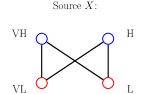
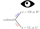
Figure 1: (a) From the supervisor’s perspective, symbols ${\rm VH}$ (very high) and ${\rm H}$ (high) are indistinguishable (i.e., need not to be distinguished), and so are symbols ${\rm VL}$ (very low) and ${\rm L}$ (low). We draw an edge between any two distinguishable symbols, and then to satisfy the supervisor, we can only map non-adjacent symbols to the same codeword. (b) An adversary eavesdrops the codeword, based upon which it guesses the exact water level.

The source coding model we consider was originally introduced by Körner [2], where a vanishing error probability is allowed and the resulted optimal compression rate is defined as the graph entropy of the confusion graph. More recently, Wang and Shayevitz [3] analyzed the joint source-channel coding problem based on the same zero-error graph-theoretic setting as our model for the source coding.

Suppose that the transmitted codeword is eavesdropped by a guessing adversary, who knows the source distribution $P_{X}$ and tries to guess the true source sequence via maximum likelihood estimation within a certain number of trials. See Figure 1 for an example. Before observing the codeword, the adversary will guess the most likely water level among all four levels. After observing the codeword, say “blue”, it will guess the more likely water level between ${\rm VH}$ and $\rm H$. Compared with guessing blindly (i.e., based only on $P_{X}$), the average successful guessing probability will increase as the adversary eavesdrops the codeword. We measure the information leakage from the codeword to the adversary by such a probability increase. More specifically, the leakage is quantified as the ratio between the adversary’s probability of successful guessing after and before observing the codeword. This way of measuring information leakage was originally introduced by Smith [4], leading to the leakage metric commonly referred to as min-entropy leakage.

Quite often in practice, the compression scheme is designed without knowing the exact source distribution. In such case, one can consider the worst-case leakage, which is the information leakage maximized over all possible source distributions $P_{X}$ over the fixed alphabet $\mathcal{X}$. The worst-case variant of min-entropy leakage, namely the maximum min-entropy leakage, was developed by Braun et al. [5].

A similar idea was independently explored by Issa et al. [6, 7] in a different setup where the adversary is interested in guessing some randomized function $U$ of $X$ rather than $X$ itself. The worst-case metric under such scenario is named as the maximal leakage. Interestingly, despite their different operational meanings, the maximal leakage and maximum min-entropy leakage turn out to be equal. For more works studying the maximal leakage or the maximum min-entropy leakage and their variants from both the information-theoretic and computer science perspectives, see [8, 9, 10, 11, 12, 13, 14, 15, 16, 17]. In another related work by Shkel and Poor [18], leakage in compression systems has been studied considering multiple leakage metrics, including the maximal leakage, under the assumption that the source code must be deterministic yet a random secret key is shared between the sender and the receiver.

Clearly we wish to keep the information leakage as small as possible by smartly designing a (possibly stochastic) source coding scheme. Therefore, our fundamental objective is to characterize the minimum leakage (normalized to the source sequence length) under the zero-error decoding requirement and also the optimum-achieving mapping scheme.

Contributions and organization: In Section II, we detail the problem of information leakage in source coding. In particular, we start with the basic adversarial model where the adversary makes a single guess and allows no distortion, and thus the resulting privacy metric is the normalized version of the maximal leakage [7] or the normalized maximum min-entropy leakage [5]. Our main contributions are as follows:

1) In Section III, we develop a single-letter characterization for the optimal normalized maximal leakage for the basic adversarial model. We also design a scalar stochastic mapping scheme that achieves this optimum. An interesting observation is that the optimal leakage can also be achieved using deterministic codes that simultaneously achieve the optimal fixed-length zero-error compression rate.

2) In Section IV, we extend our adversarial model to allow multiple guesses and distortion between an estimator (guess) and the true sequence. Inspired by the notion of confusion graphs, we characterize the relationship between a sequence and its acceptable estimators by another graph defined on the source alphabet, resulting in a novel leakage measurement.

3) We then show that the optimal normalized leakage under the generalized models is always upper-bounded by the result in the original setup. Single-letter lower bounds (i.e., converse results) are also established.

We also include a brief review on basic graph-theoretic definitions in Appendix A.

Notation: For non-negative integers $a$ and $b$, $[a]$ denotes the set $\{1,2,\dots,a\}$, and $[a\mathchar 58\relax b]$ denotes the set $\{a,a+1,\dots,b\}$. If $a>b$, $[a\mathchar 58\relax b]=\emptyset$. For a finite set $A$, $\mathchoice{\mspace{1.0mu}|\mspace{1.0mu}}{|}{|}{|}A\mathchoice{\mspace{1.0mu}|\mspace{1.0mu}}{|}{|}{|}$ denotes its cardinality. For two sets $A$ and $B$, $A\times B$ denotes their Cartesian product. For a sequence of sets $A_{1},A_{2},\dots,A_{t}$, we may simply use $\prod_{j\in[t]}A_{j}$ to denote their Cartesian product. For any discrete random variable $Z$ with probability distribution $P_{Z}$, we denote its alphabet by $\mathcal{Z}$ with realizations $z\in\mathcal{Z}$. For any $K\subseteq\mathcal{Z}$, $P_{Z}(K)\doteq\sum_{z\in K}P_{Z}(z)$.

II System Model and Problem Formulation

Source coding with confusion graph $\Gamma$: Consider a discrete memoryless stationary information source $X$ that takes values in the alphabet $\mathcal{X}$ with full support. We wish to stochastically compress a source sequence $X^{t}\doteq(X_{1},X_{2},\dots,X_{t})$ to some codeword $Y$ that takes values in the code alphabet $\mathcal{Y}$ and transmit it to a legitimate receiver via a noiseless channel. The randomized mapping scheme from $\mathcal{X}$ to $\mathcal{Y}$ is denoted by the conditional distribution $P_{Y\mathchoice{\mspace{1.0mu}|\mspace{1.0mu}}{|}{|}{|}X^{t}}$.

To the receiver, the distinguishability relationship among source symbols is characterized by a confusion graph $\Gamma$, where the vertex set is the source alphabet, i.e., $V(\Gamma)=\mathcal{X}$, and any two symbols $x,x^{\prime}\in\mathcal{X}$ are adjacent in $\Gamma$, i.e., $\{x,x^{\prime}\}\in\mathcal{E}(\Gamma)$, iff they are distinguishable with each other. Any two source sequences, $x^{t}=(x_{1},\dots,x_{t})\in\mathcal{X}^{t}$ and $v^{t}=(v_{1},\dots,v_{t})\in\mathcal{X}^{t}$, are distinguishable iff at some $j\in[t]$, $x_{j}$ and $v_{j}$ are distinguishable. Therefore, the distinguishability among source sequences of length $t$ is characterized by the confusion graph $\Gamma_{t}$, which is defined as the $t$-th power of $\Gamma$ with respect to the OR (disjunctive) graph product [19, Section 3.4]: $\Gamma_{t}=\Gamma\lor\Gamma\lor\dots\lor\Gamma=\Gamma^{\lor t}$.

To ensure zero-error decoding, any two source sequences that can be potentially mapped to the same codeword must not be distinguishable. More formally, given some $P_{Y\mathchoice{\mspace{1.0mu}|\mspace{1.0mu}}{|}{|}{|}X^{t}}$, let

$$\mathcal{X}^{t}_{P_{Y\mathchoice{\mspace{1.0mu}|\mspace{1.0mu}}{|}{|}{|}X^{t}}}(y)\doteq\{x^{t}\in\mathcal{X}^{t}\mathchar 58\relax P_{Y\mathchoice{\mspace{1.0mu}|\mspace{1.0mu}}{|}{|}{|}X^{t}}(y\mathchoice{\mspace{1.0mu}|\mspace{1.0mu}}{|}{|}{|}x^{t})>0\}$$ (1)

denote the set of all $x^{t}$ mapped to $y$ with nonzero probability. When there is no ambiguity, we simply denote $\mathcal{X}^{t}_{P_{Y\mathchoice{\mspace{1.0mu}|\mspace{1.0mu}}{|}{|}{|}X^{t}}}(y)$ by $\mathcal{X}^{t}(y)$. Therefore, a mapping scheme $P_{Y\mathchoice{\mspace{1.0mu}|\mspace{1.0mu}}{|}{|}{|}X^{t}}$ is valid iff

$$\mathcal{X}^{t}(y)\in\mathcal{I}(\Gamma_{t}),\quad\forall y\in\mathcal{Y},$$ (2)

where $\mathcal{I}(\cdot)$ denotes the set of independent sets of a graph (cf. Appendix A).

Leakage to a guessing adversary: As a starting point, we assume that the adversary makes a single guess after observing each codeword and allows no distortion between its estimator sequence and the true source sequence.

Consider any source coding problem $\Gamma$. The maximal leakage for a given sequence length $t$ and a given valid mapping $P_{Y\mathchoice{\mspace{1.0mu}|\mspace{1.0mu}}{|}{|}{|}X^{t}}$ is defined as follows:

$$L^{t}(P_{Y\mathchoice{\mspace{1.0mu}|\mspace{1.0mu}}{|}{|}{|}X^{t}}) \doteq\log\max_{P_{X}}\frac{{\mathbb{E}}_{Y}\left[\max\limits_{x^{t}\in\mathcal{X}^{t}}P_{X^{t}\mathchoice{\mspace{1.0mu}|\mspace{1.0mu}}{|}{|}{|}Y}(x^{t}\mathchoice{\mspace{1.0mu}|\mspace{1.0mu}}{|}{|}{|}Y)\right]}{\max\limits_{x^{t}\in\mathcal{X}^{t}}P_{X^{t}}(x^{t})}$$ (3)

$$=\log\max_{P_{X}}\frac{\sum\limits_{y\in\mathcal{Y}}\max\limits_{x^{t}\in\mathcal{X}^{t}}P_{X^{t},Y}(x^{t},y)}{\max\limits_{x^{t}\in\mathcal{X}^{t}}P_{X^{t}}(x^{t})}$$ (4)

$$=\log\sum\limits_{y\in\mathcal{Y}}\max\limits_{x^{t}\in\mathcal{X}^{t}}P_{Y\mathchoice{\mspace{1.0mu}|\mspace{1.0mu}}{|}{|}{|}X^{t}}(y\mathchoice{\mspace{1.0mu}|\mspace{1.0mu}}{|}{|}{|}x^{t}),$$ (5)

where $\eqref{eq:def:max:leakage:rate:simplified:any:t:mapping}$ follows from [5, Proposition 5.1]. The optimal maximal leakage for a given $t$ is then defined as

$$\mathcal{L}^{t} \doteq\inf_{\begin{subarray}{c}P_{Y\mathchoice{\mspace{1.0mu}|\mspace{1.0mu}}{|}{|}{|}X^{t}}\mathchar 58\relax\\ {\color[rgb]{0,0,0}\mathcal{X}^{t}(y)\in\mathcal{I}(\Gamma_{t})},\forall y\in\mathcal{Y}\end{subarray}}L^{t}(P_{Y\mathchoice{\mspace{1.0mu}|\mspace{1.0mu}}{|}{|}{|}X^{t}}),$$ (6)

based upon which we can define the (optimal) maximal leakage rate as

$$\mathcal{L} \doteq\lim_{t\to\infty}t^{-1}\mathcal{L}^{t}.$$ (7)

III Maximal Leakage Rate: Characterization

In the following we present a single-letter characterization of the maximal leakage rate $\mathcal{L}$.

Theorem 1

For any source coding problem $\Gamma$,

$$\mathcal{L}=\log\chi_{f}(\Gamma),$$ (8)

where $\chi(\cdot)$ denotes the fractional chromatic number of a graph (cf. Definition 4).

To prove Theorem 1, we introduce several useful lemmas.

We first show that given any mapping scheme, “merging” any two codewords does not increase the leakage (as long as the generated mapping is still valid).

More precisely, consider any sequence length $t$ and any valid mapping $P_{Y\mathchoice{\mspace{1.0mu}|\mspace{1.0mu}}{|}{|}{|}X^{t}}$ such that there exists some mergeable codewords $y_{1},y_{2}\in\mathcal{Y}$, $y_{1}\neq y_{2}$, satisfying $\mathcal{X}^{t}(y_{1})\cup\mathcal{X}^{t}(y_{2})\subseteq T$ for some $T\in\mathcal{I}_{\rm max}(\Gamma_{t})$, where $\mathcal{I}_{\rm max}(\cdot)$ denotes the set of maximal independent sets of a graph (cf. Appendix A). Construct $P_{Y_{1,2}\mathchoice{\mspace{1.0mu}|\mspace{1.0mu}}{|}{|}{|}X^{t}}$ by merging $y_{1}$ and $y_{2}$ to a new codeword $y_{1,2}\notin\mathcal{Y}$. That is, $\mathcal{Y}_{1,2}=(\mathcal{Y}\setminus\{y_{1},y_{2}\})\cup\{y_{1,2}\}$, and for any $x^{t}\in\mathcal{X}^{t}$,

$$P_{Y_{1,2}\mathchoice{\mspace{1.0mu}|\mspace{1.0mu}}{|}{|}{|}X^{t}}(y\mathchoice{\mspace{1.0mu}|\mspace{1.0mu}}{|}{|}{|}x^{t})$$

$$=\begin{cases}P_{Y\mathchoice{\mspace{1.0mu}|\mspace{1.0mu}}{|}{|}{|}X^{t}}(y_{1}\mathchoice{\mspace{1.0mu}|\mspace{1.0mu}}{|}{|}{|}x^{t})+P_{Y\mathchoice{\mspace{1.0mu}|\mspace{1.0mu}}{|}{|}{|}X^{t}}(y_{2}\mathchoice{\mspace{1.0mu}|\mspace{1.0mu}}{|}{|}{|}x^{t}),\quad\enskip\text{if $y=y_{1,2}$},\\ P_{Y\mathchoice{\mspace{1.0mu}|\mspace{1.0mu}}{|}{|}{|}X^{t}}(y\mathchoice{\mspace{1.0mu}|\mspace{1.0mu}}{|}{|}{|}x^{t}),\qquad\qquad\qquad\qquad\enskip\text{otherwise}.\end{cases}$$ (9)

Then we have the following result.

Lemma 1

$L^{t}(P_{Y_{1,2}\mathchoice{\mspace{1.0mu}|\mspace{1.0mu}}{|}{|}{|}X^{t}})\leq L^{t}(P_{Y\mathchoice{\mspace{1.0mu}|\mspace{1.0mu}}{|}{|}{|}X^{t}})$.

Proof:

It suffices to show $\max_{x^{t}\in\mathcal{X}^{t}}P_{Y_{1,2}\mathchoice{\mspace{1.0mu}|\mspace{1.0mu}}{|}{|}{|}X^{t}}(y_{1,2}\mathchoice{\mspace{1.0mu}|\mspace{1.0mu}}{|}{|}{|}x^{t})$ being no larger than $\sum_{y\in\{y_{1},y_{2}\}}\max_{x^{t}\in\mathcal{X}^{t}}P_{Y\mathchoice{\mspace{1.0mu}|\mspace{1.0mu}}{|}{|}{|}X^{t}}(y\mathchoice{\mspace{1.0mu}|\mspace{1.0mu}}{|}{|}{|}x^{t})$ as

$$\max_{x^{t}\in\mathcal{X}^{t}}P_{Y_{1,2}\mathchoice{\mspace{1.0mu}|\mspace{1.0mu}}{|}{|}{|}X^{t}}(y_{1,2}\mathchoice{\mspace{1.0mu}|\mspace{1.0mu}}{|}{|}{|}x^{t})$$

$$=\max_{x^{t}\in\mathcal{X}^{t}}(P_{Y\mathchoice{\mspace{1.0mu}|\mspace{1.0mu}}{|}{|}{|}X^{t}}(y_{1}\mathchoice{\mspace{1.0mu}|\mspace{1.0mu}}{|}{|}{|}x^{t})+P_{Y\mathchoice{\mspace{1.0mu}|\mspace{1.0mu}}{|}{|}{|}X^{t}}(y_{2}\mathchoice{\mspace{1.0mu}|\mspace{1.0mu}}{|}{|}{|}x^{t}))$$

$$\leq\max_{x^{t}\in\mathcal{X}^{t}}P_{Y\mathchoice{\mspace{1.0mu}|\mspace{1.0mu}}{|}{|}{|}X^{t}}(y_{1}\mathchoice{\mspace{1.0mu}|\mspace{1.0mu}}{|}{|}{|}x^{t})+\max_{x^{t}\in\mathcal{X}^{t}}P_{Y\mathchoice{\mspace{1.0mu}|\mspace{1.0mu}}{|}{|}{|}X^{t}}(y_{2}\mathchoice{\mspace{1.0mu}|\mspace{1.0mu}}{|}{|}{|}x^{t})$$

$$=\sum_{y\in\{y_{1},y_{2}\}}\max_{x^{t}\in\mathcal{X}^{t}}P_{Y\mathchoice{\mspace{1.0mu}|\mspace{1.0mu}}{|}{|}{|}X^{t}}(y\mathchoice{\mspace{1.0mu}|\mspace{1.0mu}}{|}{|}{|}x^{t}),$$

which completes the proof of the lemma. ∎

As specified in (2), for a valid mapping scheme, every codeword $y$ should correspond to an independent set of the confusion graph $\Gamma$. As a consequence of Lemma 1, to characterize the optimal leakage, it suffices to consider only those mapping schemes for which all codewords $y$ correspond to distinct maximal independent sets of $\Gamma$.

To formalize this observation, for any sequence length $t$, define the distortion function $d_{t}\mathchar 58\relax\mathcal{X}^{t}\times\mathcal{I}_{\rm max}(\Gamma_{t})\to\{0,1\}$ such that for any $x^{t}\in\mathcal{X}^{t}$, $T\in\mathcal{I}_{\rm max}(\Gamma_{t})$,

$$d(x^{t},y)=\begin{cases}0,\quad x^{t}\in T,\\ 1,\quad x^{t}\notin T.\end{cases}$$ (10)

Then the lemma below holds, whose proof is presented in Appendix B.

Lemma 2

To characterize $\mathcal{L}^{t}$ defined in (6), it suffices to assume the mapping $P_{Y\mathchoice{\mspace{1.0mu}|\mspace{1.0mu}}{|}{|}{|}X^{t}}$ to satisfy that $\mathcal{Y}=\mathcal{I}_{\rm max}(\Gamma_{t})$ and $d(X^{t},Y)=0$ almost surely. Thus by (5), we have

$$\mathcal{L}^{t} =\inf_{\begin{subarray}{c}P_{Y\mathchoice{\mspace{1.0mu}|\mspace{1.0mu}}{|}{|}{|}X^{t}}\mathchar 58\relax\\ \mathcal{Y}=\mathcal{I}_{\rm max}(\Gamma_{t}),\\ d(X^{t},Y)=0\end{subarray}}\log\sum_{y\in\mathcal{Y}}\max_{x^{t}\in\mathcal{X}^{t}}P_{Y\mathchoice{\mspace{1.0mu}|\mspace{1.0mu}}{|}{|}{|}X^{t}}(y\mathchoice{\mspace{1.0mu}|\mspace{1.0mu}}{|}{|}{|}x^{t}).$$ (11)

The solution to the optimization problem on the right hand side of (11) in Lemma 2 is characterized by [20, Corollary 1], based upon which we have the following result.

Lemma 3

$\mathcal{L}^{t}=-\log\eta,$ where $\eta$ is the solution to the following maximin problem:

maximize $$\min_{x^{t}\in\mathcal{X}^{t}}\sum_{T\in\mathcal{I}_{\rm max}(\Gamma_{t})\mathchar 58\relax x^{t}\in T}\kappa_{T},$$ (12a)

subject to $$\sum_{T\in\mathcal{I}_{\rm max}(\Gamma_{t})}\kappa_{T}=1,$$ (12b)

$$\kappa_{T}\in[0,1],\quad\forall T\in\mathcal{I}_{\rm max}(\Gamma_{t}).$$ (12c)

On the other hand, for any $t$, $\chi_{f}(\Gamma_{t})$ is the solution to the following linear program [21, Section 2.2]:

minimize $$\sum_{T\in\mathcal{I}_{\rm max}(\Gamma_{t})}\lambda_{T},$$ (13a)

subject to $$\sum_{T\in\mathcal{I}_{\rm max}(\Gamma_{t})\mathchar 58\relax x^{t}\in T}\lambda_{T}\geq 1,\quad\forall x^{t}\in\mathcal{X}^{t},$$ (13b)

$$\lambda_{T}\in[0,1],\quad\forall T\in\mathcal{I}_{\rm max}(\Gamma_{t}).$$ (13c)

We can show that the solutions to the optimization problems (12) and (13) are reciprocal to each other. That is,

$$\eta=\frac{1}{\chi_{f}(\Gamma_{t})},$$ (14)

whose proof is presented in Appendix C. The remaining proof of Theorem 1 follows easily from the above results.

Proof:

We have

$$\mathcal{L} \stackrel{{\scriptstyle\mathchoice{\hbox to0.0pt{\hss$\displaystyle{(a)}$\hss}}{\hbox to0.0pt{\hss$\textstyle{(a)}$\hss}}{\hbox to0.0pt{\hss$\scriptstyle{(a)}$\hss}}{\hbox to0.0pt{\hss$\scriptscriptstyle{(a)}$\hss}}}}{{=}}\lim_{t\to\infty}\frac{1}{t}(-\log\eta)\stackrel{{\scriptstyle\mathchoice{\hbox to0.0pt{\hss$\displaystyle{(b)}$\hss}}{\hbox to0.0pt{\hss$\textstyle{(b)}$\hss}}{\hbox to0.0pt{\hss$\scriptstyle{(b)}$\hss}}{\hbox to0.0pt{\hss$\scriptscriptstyle{(b)}$\hss}}}}{{=}}\lim_{t\to\infty}\frac{1}{t}\log\chi_{f}(\Gamma_{t})\stackrel{{\scriptstyle\mathchoice{\hbox to0.0pt{\hss$\displaystyle{(c)}$\hss}}{\hbox to0.0pt{\hss$\textstyle{(c)}$\hss}}{\hbox to0.0pt{\hss$\scriptstyle{(c)}$\hss}}{\hbox to0.0pt{\hss$\scriptscriptstyle{(c)}$\hss}}}}{{=}}\log\chi_{f}(\Gamma).$$

where (a) follows from (7) and Lemma 3, (b) follows (14), and (c) follows from the fact that $\chi_{f}(\Gamma_{t})=\chi_{f}(\Gamma^{\lor t})=\chi_{f}(\Gamma)^{t}$ (cf. [19, Corollary 3.4.2]). ∎

Having characterized the optimal maximal leakage rate $\mathcal{L}$ in Theorem 1, in the following we design an optimal mapping scheme $P_{Y\mathchoice{\mspace{1.0mu}|\mspace{1.0mu}}{|}{|}{|}X^{t}}$ for some $t$ that achieves $\mathcal{L}$, which is based on the optimal fractional coloring of the confusion graph $\Gamma$.

Fix the sequence length $t=1$. For $\Gamma_{1}=\Gamma$, there always exists some $b$-fold coloring $\mathcal{P}=\{T_{1},T_{2},\dots,T_{m}\}$ for some finite positive integer $b$ such that $\chi_{f}(\Gamma)=m/b$ (cf. Definitions 3 and 4; see also [19, Corollary 1.3.2 and Section 3.1]).

Set $\mathcal{Y}=\mathcal{P}$ (and thus every codeword $y\in\mathcal{Y}$ is actually an independent set of $\Gamma$). Set

$$P_{Y\mathchoice{\mspace{1.0mu}|\mspace{1.0mu}}{|}{|}{|}X}(y\mathchoice{\mspace{1.0mu}|\mspace{1.0mu}}{|}{|}{|}x)=\begin{cases}1/b,\quad\text{if $x\in y$},\\ 0,\qquad\text{otherwise.}\end{cases}$$ (15)

As every $x\in\mathcal{X}$ is in exactly $b$ sets within $\mathcal{P}$, we have

$$\sum_{y\in\mathcal{Y}}P_{Y\mathchoice{\mspace{1.0mu}|\mspace{1.0mu}}{|}{|}{|}X}(y\mathchoice{\mspace{1.0mu}|\mspace{1.0mu}}{|}{|}{|}x)=\sum_{y\in\mathcal{Y}\mathchar 58\relax x\in y}\frac{1}{b}+\sum_{y\in\mathcal{Y}\mathchar 58\relax x\notin y}0=1,\quad\forall x\in\mathcal{X},$$

and thus $P_{Y\mathchoice{\mspace{1.0mu}|\mspace{1.0mu}}{|}{|}{|}X}$ is a valid mapping scheme. We have

$$L^{1}(P_{Y\mathchoice{\mspace{1.0mu}|\mspace{1.0mu}}{|}{|}{|}X}) =\log\sum_{y\in\mathcal{Y}}\max_{x\in\mathcal{X}}P_{Y\mathchoice{\mspace{1.0mu}|\mspace{1.0mu}}{|}{|}{|}X}(y\mathchoice{\mspace{1.0mu}|\mspace{1.0mu}}{|}{|}{|}x)$$

$$=\log\sum_{y\in\mathcal{P}}\frac{1}{b}=\log\frac{m}{b}=\log\chi_{f}(\Gamma),$$ (16)

and thus we know that the maximal leakage rate in Theorem 1 is indeed achievable by the mapping described in (15).

Remark 1

Consider any source coding problem $\Gamma$. We know that the optimal zero-error compression rate (with fixed-length deterministic source codes) is

$$\mathcal{R} =\lim_{t\to\infty}\frac{1}{t}\log\chi(\Gamma^{\lor t})=\lim_{t\to\infty}\frac{1}{t}\log\chi_{f}(\Gamma^{\lor t})=\log\chi_{f}(\Gamma),$$

where the second equality follows from [19, Corollary 3.4.3]. We can verify that the above result holds even when we allow stochastic mapping. Hence, the maximal leakage rate $\mathcal{L}$ always equals to the optimal compression rate $\mathcal{R}$. Moreover, it can be verified that any $\mathcal{R}$-achieving deterministic code can simultaneously achieve $\mathcal{L}$. In other words, when considering fixed-length source coding, there is no trade-off between the compression rate and the leakage rate. Furthermore, we observe the following:

1. Our characterization of $\mathcal{L}$ holds generally and does not rely on the assumption of fixed-length coding;

2. While in general, the optimal zero-error compression rate $\mathcal{R}$ and the maximal leakage rate $\mathcal{L}$ can be simultaneously and asymptotically attained at the limit of increasing $t$, we showed in (16) that $\mathcal{L}$, on the other hand, can be achieved exactly even with $t=1$ (using the symbol-by-symbol encoding scheme specified in (15) based on the factional coloring of $\Gamma$), but possibly at the expense of the compression rate.

3. For variable-length source coding, whether there is a compression-leakage trade-off remains unclear.

IV Extensions on the Maximal Leakage Rate: Multiple and Approximate Guesses

In general, the adversary may be able to make multiple guesses. For example, the adversary may possess a testing mechanism to verify whether its guess is correct or not, and thus can perform a trial and error attack until it is stopped by the system. Also, for each true source sequence, there may be multiple estimators other than the true sequence itself that are “close enough” and thus can be regarded successful.

We generalize our definition of information leakage to cater to the above scenarios. Consider any source coding problem $\Gamma$, sequence length $t$, and valid mapping $P_{Y\mathchoice{\mspace{1.0mu}|\mspace{1.0mu}}{|}{|}{|}X^{t}}$. Suppose the adversary generates a set of guesses $K\subseteq\mathcal{X}^{t}$. For each set $K$, define a “covering” set $K^{+}$, where $K\subseteq K^{+}\subseteq\mathcal{X}^{t}$, such that if the true sequence is in $K^{+}$, then the adversary’s guess list $K$ is considered successful. Let

$$\mathcal{S}\doteq\{K^{+}\mathchar 58\relax\text{$K$ is a guess list the adversary can choose}\}$$

be the collection of all possible $K^{+}$. Then for the blind guessing, the successful probability is $\max_{S\in\mathcal{S}}\sum_{x^{t}\in S}P_{X^{t}}(x^{t}),$ and for guessing after observing $Y$, the average successful probability is ${\mathbb{E}}_{Y}\left[\max_{S\in\mathcal{S}}\sum_{x^{t}\in S}P_{X^{t}\mathchoice{\mspace{1.0mu}|\mspace{1.0mu}}{|}{|}{|}Y}(x^{t}\mathchoice{\mspace{1.0mu}|\mspace{1.0mu}}{|}{|}{|}Y)\right].$ In the same spirit of maximal leakage, we can define

$$\rho_{t}(P_{Y\mathchoice{\mspace{1.0mu}|\mspace{1.0mu}}{|}{|}{|}X^{t}},\mathcal{S}) \doteq\log\max_{P_{X}}\frac{{\mathbb{E}}_{Y}\left[\max\limits_{S\in\mathcal{S}}\sum\limits_{x^{t}\in S}P_{X^{t}\mathchoice{\mspace{1.0mu}|\mspace{1.0mu}}{|}{|}{|}Y}(x^{t}\mathchoice{\mspace{1.0mu}|\mspace{1.0mu}}{|}{|}{|}Y)\right]}{\max\limits_{S\in\mathcal{S}}\sum\limits_{x^{t}\in S}P_{X^{t}}(x^{t})}$$

as the ratio between the a posteriori and a priori successful guessing probability. If we set $\mathcal{S}_{\rm singleton}=\{\{x^{t}\}\mathchar 58\relax x^{t}\in\mathcal{X}^{t}\}$, that is, the adversary is allowed one guess and it must guess the correct source sequence precisely, the maximal leakage defined in (3) can be equivalently written as

$$L^{t}(P_{Y\mathchoice{\mspace{1.0mu}|\mspace{1.0mu}}{|}{|}{|}X^{t}}) =\rho_{t}(P_{Y\mathchoice{\mspace{1.0mu}|\mspace{1.0mu}}{|}{|}{|}X^{t}},\mathcal{S}_{\rm singleton}).$$

In the next three subsections, we study the information leakage rate under different adversarial models.

IV-A Leakage for the Case of Multiple Guesses

In this subsection, we consider the case where the adversary make multiple guesses, yet does not allow distortion between its estimators and the true sequence.

We characterize the number of guesses the adversary can make by a guessing capability function $g(t)$, where $t\in{\mathbb{Z}}^{+}$ is the sequence length. We assume $g(t)$ to be positive, integer-valued, non-decreasing, and upper-bounded by $\alpha(\Gamma_{t})=\alpha(\Gamma^{\lor t})=\alpha(\Gamma)^{t}$, where $\alpha(\cdot)$ denotes the independence number of a graph (cf. Appendix A).

Consider any source coding problem $\Gamma$ and any guessing-capability function $g$. For a given sequence length $t$ and a given valid mapping $P_{Y\mathchoice{\mspace{1.0mu}|\mspace{1.0mu}}{|}{|}{|}X^{t}}$, the maximal leakage naturally extends to the multi-guess maximal leakage, defined as

$$L^{t}_{g}(P_{Y\mathchoice{\mspace{1.0mu}|\mspace{1.0mu}}{|}{|}{|}X^{t}})\doteq\rho_{t}(P_{Y\mathchoice{\mspace{1.0mu}|\mspace{1.0mu}}{|}{|}{|}X^{t}},\mathcal{S}_{g}),$$ (17)

where $\mathcal{S}_{g}=\{K\subseteq\mathcal{X}^{t}\mathchar 58\relax\mathchoice{\mspace{1.0mu}|\mspace{1.0mu}}{|}{|}{|}K\mathchoice{\mspace{1.0mu}|\mspace{1.0mu}}{|}{|}{|}=g(t)\}$. Then we can define the (optimal) multi-guess maximal leakage rate as

$$\mathcal{L}_{g} \doteq\lim_{t\to\infty}\frac{1}{t}\inf_{\begin{subarray}{c}P_{Y\mathchoice{\mspace{1.0mu}|\mspace{1.0mu}}{|}{|}{|}X^{t}}\mathchar 58\relax\\ {\color[rgb]{0,0,0}\mathcal{X}^{t}(y)\in\mathcal{I}(\Gamma_{t})},\forall y\in\mathcal{Y}\end{subarray}}L^{t}_{g}(P_{Y\mathchoice{\mspace{1.0mu}|\mspace{1.0mu}}{|}{|}{|}X^{t}}).$$ (18)

We first show that the multi-guess maximal leakage rate is always no larger than the maximal leakage.

Lemma 4

For any source coding problem $\Gamma$ and guessing capability function $g$, we have $\mathcal{L}_{g}\leq\mathcal{L}$.

Proof:

It suffices to show $L_{g}^{t}(P_{Y\mathchoice{\mspace{1.0mu}|\mspace{1.0mu}}{|}{|}{|}X^{t}})\leq L^{t}(P_{Y\mathchoice{\mspace{1.0mu}|\mspace{1.0mu}}{|}{|}{|}X^{t}})$ for any $t$ and $P_{Y\mathchoice{\mspace{1.0mu}|\mspace{1.0mu}}{|}{|}{|}X^{t}}$. For any $P_{X}$, we have

$$\frac{\sum\limits_{y\in\mathcal{Y}}\max\limits_{K\subseteq\mathcal{X}^{t}\mathchar 58\relax\mathchoice{\mspace{1.0mu}|\mspace{1.0mu}}{|}{|}{|}K\mathchoice{\mspace{1.0mu}|\mspace{1.0mu}}{|}{|}{|}=g(t)}\sum\limits_{x^{t}\in K}P_{X^{t},Y}(x^{t},y)}{\max\limits_{\begin{subarray}{c}K\subseteq\mathcal{X}^{t}\mathchar 58\relax\mathchoice{\mspace{1.0mu}|\mspace{1.0mu}}{|}{|}{|}K\mathchoice{\mspace{1.0mu}|\mspace{1.0mu}}{|}{|}{|}=g(t)\end{subarray}}\sum_{x^{t}\in K}P_{X^{t}}(x^{t})}$$

$$\leq\frac{\sum\limits_{y\in\mathcal{Y}}\big{(}\max\limits_{K\subseteq\mathcal{X}^{t}\mathchar 58\relax\mathchoice{\mspace{1.0mu}|\mspace{1.0mu}}{|}{|}{|}K\mathchoice{\mspace{1.0mu}|\mspace{1.0mu}}{|}{|}{|}=g(t)}\sum\limits_{x^{t}\in K}P_{X^{t}}(x^{t})\big{)}\big{(}\max\limits_{{\tilde{x}}^{t}\in\mathcal{X}^{t}}P_{Y\mathchoice{\mspace{1.0mu}|\mspace{1.0mu}}{|}{|}{|}X^{t}}(y\mathchoice{\mspace{1.0mu}|\mspace{1.0mu}}{|}{|}{|}{\tilde{x}}^{t})\big{)}}{\max\limits_{\begin{subarray}{c}K\subseteq\mathcal{X}^{t}\mathchar 58\relax\mathchoice{\mspace{1.0mu}|\mspace{1.0mu}}{|}{|}{|}K\mathchoice{\mspace{1.0mu}|\mspace{1.0mu}}{|}{|}{|}=g(t)\end{subarray}}\sum_{x^{t}\in K}P_{X^{t}}(x^{t})}$$

$$=\sum_{y\in\mathcal{Y}}\max_{x^{t}\in\mathcal{X}^{t}}P_{Y\mathchoice{\mspace{1.0mu}|\mspace{1.0mu}}{|}{|}{|}X^{t}}(y\mathchoice{\mspace{1.0mu}|\mspace{1.0mu}}{|}{|}{|}x^{t}),$$

which implies that $L_{g}^{t}(P_{Y\mathchoice{\mspace{1.0mu}|\mspace{1.0mu}}{|}{|}{|}X^{t}})\leq L^{t}(P_{Y\mathchoice{\mspace{1.0mu}|\mspace{1.0mu}}{|}{|}{|}X^{t}})$. ∎

We have the following single-letter lower and upper bounds on $\mathcal{L}_{g}$, whose proof is presented in Appendix D.

Theorem 2

We have

$$\log\mathchoice{\mspace{1.0mu}|\mspace{1.0mu}}{|}{|}{|}V(\Gamma)\mathchoice{\mspace{1.0mu}|\mspace{1.0mu}}{|}{|}{|}-\log\alpha(\Gamma)\leq\mathcal{L}_{g}\leq\log\chi_{f}(\Gamma).$$ (19)

When the adversary guesses some randomized function $U$ of $X$ rather than $X$ itself, the maximal leakage equals to its multi-guess extension [7]. It remains to be investigated whether a similar equivalence holds generally in our setup. In the following we recognize one special case where indeed $\mathcal{L}_{g}=\mathcal{L}$ and consequently, by Theorem 1, $\mathcal{L}_{g}=\log\chi_{f}(\Gamma)$.

Proposition 1

Consider any source coding problem $\Gamma$. If $\lim_{t\to\infty}\frac{1}{t}\log g(t)=0$, then $\mathcal{L}_{g}=\mathcal{L}=\log\chi_{f}(\Gamma)$.

The proof of the above proposition is relegated to Appendix E. Intuitively, the above result suggests that when the number of guesses the adversary can make does not grow “fast enough” with respect to $t$, it makes no difference whether the adversary is making one guess or multiple guesses (in terms of the leakage defined in (7) and (18)).

As a direct corollary of Theorem 2, the result below shows that $\mathcal{L}_{g}=\mathcal{L}=\log\chi_{f}(\Gamma)$ holds for another specific scenario.

Corollary 1

If $\Gamma$ is vertex-transitive [19, Section 1.3], then $\mathcal{L}_{g}=\mathcal{L}=\log\chi_{f}(\Gamma)$ for any function $g$.

Proof:

Since $\Gamma$ is vertex-transitive, by [19, Proposition 3.1.1], we have $\chi_{f}(\Gamma)=\mathchoice{\mspace{1.0mu}|\mspace{1.0mu}}{|}{|}{|}V(\Gamma)\mathchoice{\mspace{1.0mu}|\mspace{1.0mu}}{|}{|}{|}/\alpha(\Gamma)$, which indicates that lower and upper bounds in Theorem 2 match with each other, thus establishing $\mathcal{L}_{g}=\log\chi_{f}(\Gamma)=\mathcal{L}$. ∎

IV-B Leakage for the Case of One Approximate Guess

Suppose that the adversary makes only one guess yet allows a certain level of distortion between its estimator and the true source value. That is, the guess is regarded successful as long as the estimator is an acceptable approximation to the true value. Inspired by the notion of confusion graph $\Gamma$ that characterizes the distinguishability within the source symbols, we introduce another graph to characterize the approximation relationship among source symbols (from the adversary’s perspective). We call this graph the adversary’s approximation graph, or simply the approximation graph, denoted by $\Theta$. The vertex set of $\Theta$ is just the source alphabet, i.e., $V(\Theta)=\mathcal{X}$, and any two source symbols $x\neq x^{\prime}\in\mathcal{X}$ are acceptable approximations to each other iff they are adjacent in $\Theta$, i.e., $\{x,x^{\prime}\}\in\mathcal{E}(\Theta)$.

Given a sequence length $t$, any two sequences $x^{t}=(x_{1},\ldots,x_{t})$ and $v^{t}=(v_{1},\dots,v_{t})$ are acceptable approximations to each other iff for every $j\in[t]$, $x_{j}=v_{j}$ or $\{x_{j},v_{j}\}\in\mathcal{E}(\Theta)$. Hence the approximation graph $\Theta_{t}$ for sequence length $t$ is the $t$-th power of $\Theta$ with respect to the AND graph product [22, Section 5.2]: $\Theta_{t}={\Theta\boxtimes\Theta\boxtimes\cdots\boxtimes\Theta}=\Theta^{\boxtimes t}$.

For any vertex $x^{t}\in\mathcal{X}^{t}$, let $N(\Theta_{t},x^{t})$ denote the neighborhood of $x^{t}$ within $\Theta_{t}$, including the vertex $x^{t}$ itself. That is, $N(\Theta_{t},x^{t})=\{v^{t}\in\mathcal{X}^{t}\mathchar 58\relax\text{$v^{t}=x^{t}$ or $\{v^{t},x^{t}\}\in\mathcal{E}(\Theta_{t})$}\}$.

Consider any source coding problem $\Gamma$ and any approximation graph $\Theta$. For a given sequence length $t$ and a given valid mapping $P_{Y\mathchoice{\mspace{1.0mu}|\mspace{1.0mu}}{|}{|}{|}X^{t}}$, the maximal leakage naturally extends to the approximate-guess maximal leakage, defined as

$$L^{t}_{\Theta}(P_{Y\mathchoice{\mspace{1.0mu}|\mspace{1.0mu}}{|}{|}{|}X^{t}})\doteq\rho_{t}(P_{Y\mathchoice{\mspace{1.0mu}|\mspace{1.0mu}}{|}{|}{|}X^{t}},\mathcal{S}_{\Theta}),$$ (20)

where $\mathcal{S}_{\Theta}=\{N(\Theta_{t},x^{t})\mathchar 58\relax x^{t}\in\mathcal{X}^{t}\}.$ Then we can define the (optimal) approximate-guess maximal leakage rate as

$$\mathcal{L}_{\Theta} \doteq\lim_{t\to\infty}\frac{1}{t}\inf_{\begin{subarray}{c}P_{Y\mathchoice{\mspace{1.0mu}|\mspace{1.0mu}}{|}{|}{|}X^{t}}\mathchar 58\relax\\ {\color[rgb]{0,0,0}\mathcal{X}^{t}(y)\in\mathcal{I}(\Gamma_{t})},\forall y\in\mathcal{Y}\end{subarray}}L^{t}_{\Theta}(P_{Y\mathchoice{\mspace{1.0mu}|\mspace{1.0mu}}{|}{|}{|}X^{t}}).$$ (21)

The approximate-guess maximal leakage is always no larger than the maximal leakage as specified in lemma below, whose proof is similar to that of Lemma 4 and thus omitted.

Lemma 5

For any source coding problem $\Gamma$ and approximation graph $\Theta$, we have $\mathcal{L}_{\Theta}\leq\mathcal{L}$.

Before presenting single-letter bounds on $\mathcal{L}_{\Theta}$, we introduce the following graph-theoretic notions.

Consider any source coding problem $\Gamma$, approximation graph $\Theta$, and sequence length $t$. For any maximal independent set $T\in\mathcal{I}_{\rm max}(\Gamma_{t})$, we define its associated hypergraph (see Appendix A for basic definitions about hypergraphs).

Definition 1 (Associated Hypergraph)

Consider any sequence length $t$. For any $T\in\mathcal{I}_{\rm max}(\Gamma_{t})$, its associated hypergraph $\mathcal{H}_{t}(T)$ is defined as $V(\mathcal{H}_{t}(T))=T$ and $\mathcal{E}(\mathcal{H}_{t}(T))=\{E\subseteq T\mathchar 58\relax E\neq\emptyset,\text{$E=T\cap N(\Theta_{t},x^{t})$ for some $x^{t}\in\mathcal{X}^{t}$}\}$.

The following single-letter lower and upper bounds on $\mathcal{L}_{\Theta}$ hold, whose proof is presented in Appendix F.

Theorem 3

We have

$$\log\frac{p_{f}(\Theta)}{\max\limits_{T\in\mathcal{I}_{\rm max}(\Gamma)}k_{f}(\mathcal{H}_{1}(T))}\leq\mathcal{L}_{\Theta}\leq\log\chi_{f}(\Gamma),$$ (22)

where $p_{f}(\cdot)$ denotes the fractional closed neighborhood packing number [19, Section 7.4] of a graph and $k_{f}(\cdot)$ denotes the fractional covering number (cf. Definition 8) of a hypergraph.

Remark 2

While the lower bound in Theorem 3 takes both $\Gamma$ and $\Theta$ into account, the upper bound solely depends on $\Gamma$.

IV-C Leakage for the Case of Multiple Approximate Guesses

We consider the most generic mathematical model so far by allowing the adversary to make multiple guesses after each observation of the codeword, and a guess is regarded as successful as long as the estimated sequence is in the neighborhood of the true source sequence.

Consider any source coding problem $\Gamma$, approximation graph $\Theta$, and guessing capability function $g$. Note that we require function $g$ to be upper bounded as

$$g(t)\leq\max_{T\in\mathcal{I}_{\rm max}(\Gamma_{t})}k(\mathcal{H}_{t}(T)),\quad\forall t\in{\mathbb{Z}}^{+},$$

where $k(\cdot)$ denotes the covering number (cf. Definition 6) of a hypergraph.

For any sequence length $t$ and valid mapping $P_{Y\mathchoice{\mspace{1.0mu}|\mspace{1.0mu}}{|}{|}{|}X^{t}}$, the multi-approximate-guess maximal leakage is defined as

$$L^{t}_{\Theta,g}(P_{Y\mathchoice{\mspace{1.0mu}|\mspace{1.0mu}}{|}{|}{|}X^{t}})\doteq\rho_{t}(P_{Y\mathchoice{\mspace{1.0mu}|\mspace{1.0mu}}{|}{|}{|}X^{t}},\mathcal{S}_{\Theta,g}),$$ (23)

where $\mathcal{S}_{\Theta,g}=\{\cup_{x^{t}\in K}N(\Theta_{t},x^{t})\mathchar 58\relax K\subseteq\mathcal{X}^{t},\mathchoice{\mspace{1.0mu}|\mspace{1.0mu}}{|}{|}{|}K\mathchoice{\mspace{1.0mu}|\mspace{1.0mu}}{|}{|}{|}=g(t)\}.$ Then we can define the (optimal) multi-approximate-guess maximal leakage rate as

$$\mathcal{L}_{\Theta,g}\doteq\lim_{t\to\infty}\frac{1}{t}\inf_{\begin{subarray}{c}P_{Y\mathchoice{\mspace{1.0mu}|\mspace{1.0mu}}{|}{|}{|}X^{t}}\mathchar 58\relax\\ \mathcal{X}^{t}(y)\in\mathcal{I}(\Gamma_{t}),\forall y\in\mathcal{Y}\end{subarray}}L^{t}_{\Theta,g}(P_{Y\mathchoice{\mspace{1.0mu}|\mspace{1.0mu}}{|}{|}{|}X^{t}}).$$ (24)

Once again, following a similar proof to Lemma 4, we can show the result below.

Lemma 6

For any source coding problem $\Gamma$, approximation graph $\Theta$, and guessing capability function $g$, we have $\mathcal{L}_{\Theta,g}\leq\mathcal{L}$.

We have the following lower and upper bounds.

Theorem 4

We have

$$\log\frac{p_{f}(\Theta)}{\max\limits_{T\in\mathcal{I}_{\rm max}(\Gamma)}k_{f}(\mathcal{H}_{1}(T))}\leq L_{\Theta,g}\leq\log\chi_{f}(\Gamma),$$ (25)

The proof of the above theorem is given in Appendix G.

An interesting observation is that the lower and upper bounds for $\mathcal{L}_{\Theta,g}$ are exactly the same as the lower and upper bounds for $\mathcal{L}_{\Theta}$, respectively. However, we do not know whether $\mathcal{L}_{\Theta,g}=\mathcal{L}_{\Theta}$ holds in general.

As specified in Proposition 1, when the number of guesses the adversary can make does not grow “fast enough” with respect to $t$, or, more precisely, when $\lim_{t\to\infty}\frac{1}{t}\log g(t)=0$, the multi-guess maximal leakage rate indeed equals to the maximal leakage rate. The following lemma states that a similar equivalence holds even when the adversary allows approximation guesses.

Proposition 2

Consider any source coding problem $\Gamma$ and any approximation graph $\Theta$. For any guessing capability function $g$ such that $\lim_{t\to\infty}\frac{1}{t}\log g(t)=0$, we have $\mathcal{L}_{\Theta,g}=\mathcal{L}_{\Theta}$.

The proof is similar to that of Proposition 1 and omitted.

Appendix A Basic Graph-Theoretic Notions

Consider a directed, finite, simple, and undirected graph $G=(V,\mathcal{E})$, where $V=V(G)$ is the set of vertices of $G$ and $\mathcal{E}=\mathcal{E}(G)$ is the set of edges in $G$, which is a set of $2$-element subsets of $V$. A edge $\{v_{1},v_{2}\}\in\mathcal{E}(G)$ means that vertices $v_{1}$ and $v_{2}$ are adjacent in the graph $G$.

An independent set of $G$ is a subset of vertices $T\subseteq V$ with no edge among them. An independent set $T$ is said to be maximal iff there exists no other independent set in $G$ that is a superset of $T$. For the graph $G$, let $\mathcal{I}(G)$ denote the collection of its independent sets, and let $\mathcal{I}_{\rm max}(G)=\{T\in\mathcal{I}_{\rm max}(G)\mathchar 58\relax T\not\subseteq T^{\prime},\forall T^{\prime}\in\mathcal{I}_{\rm max}(G)\setminus\{T\}\}$ denote the collection of its maximal independent sets. Also, let $\alpha(G)$ denote the independence number of $G$, i.e., the size of the largest independent set in $G$.

We review the following basic definitions.

A multiset is a collection of elements in which each element may occur more than once [23]. The number of times an element occurs in a multiset is called its multiplicity. For example, $\{a,a,b\}$ is a multiset, where the elements $a$ and $b$ have multiplicities of $2$ and $1$, respectively. The cardinality of a multiset is the summation of the multiplicities of all its elements.

Definition 2 (Coloring and chromatic number, [19])

Given a graph $G=(V,\mathcal{E})$, a coloring of $G$ is a partition of the vertex set $V$, $\mathcal{P}=\{T_{1},T_{2},\dots,T_{m}\}$, such that for every $j\in[m]$, $T_{j}\in\mathcal{I}(G)$. The chromatic number of $G$, denoted by $\chi(G)$, is the smallest integer $m$ such that a coloring $\mathcal{P}=\{T_{1},T_{2},\dots,T_{m}\}$ exists for $G$.

Definition 3 ($b$-fold coloring and $b$-fold chromatic number, [19])

Given a graph $G=(V,\mathcal{E})$, a $b$-fold coloring of $G$ for some positive integer $b$ is a multiset $\mathcal{P}=\{T_{1},T_{2},\dots,T_{m}\}$ such that for every $j\in[m]$, $T_{j}\in\mathcal{I}(G)$, and every vertex $v\in V$ is in exactly $b$ sets in $\mathcal{P}$. The $b$-fold chromatic number of $G$, denoted by $\chi_{b}(G)$, is the smallest integer $m$ such that a $b$-fold coloring $\mathcal{P}=\{T_{1},T_{2},\dots,T_{m}\}$ exists for $G$.

Definition 4 (Fractional chromatic number, [19])

Given a graph $G=(V,\mathcal{E})$, the fractional chromatic number $\chi_{f}(G)$ is defined as

$$\chi_{f}(G)=\inf_{b}\frac{\chi_{b}(G)}{b}=\lim_{b\to\infty}\frac{\chi_{b}(G)}{b},$$

where the second equality follows from the subadditivity of $\chi_{b}(G)$ in $b$ and Fekete’s Lemma [24].

Definition 5 (Hypergraph, [19])

A hypergraph $\mathcal{H}$ consists of a vertex set $V(\mathcal{H})$ and a hyperedge set $\mathcal{E}(\mathcal{H})$, which is a family of subsets of $V(\mathcal{H})$.

It can be seen that every graph is a special hypergraph whose hyperedges are all of cardinality $2$.

For the counterparts of Definitions 2-4 for hypergraphs, see the following.

Definition 6 (Covering and covering number, [19])

Given a hypergraph $\mathcal{H}=(V,\mathcal{E})$, a covering of $\mathcal{H}$ is a set of its hyperedges, $\mathcal{P}=\{E_{1},E_{2},\dots,E_{m}\}$ where $E_{p}\in\mathcal{E},\forall p\in[m]$, such that $V=\cup_{p\in[m]}E_{p}$. The covering number of $\mathcal{H}$, denoted as $k(\mathcal{H})$, is the smallest integer $m$ such that a covering $\mathcal{P}=\{E_{1},E_{2},\dots,E_{m}\}$ exists for $\mathcal{H}$.

Definition 7 ($b$-fold covering and $b$-fold covering number, [19])

Given a hypergraph $\mathcal{H}=(V,\mathcal{E})$, a $b$-fold covering of $\mathcal{H}$ is a multiset $\mathcal{P}=\{E_{1},E_{2},\dots,E_{m}\}$ where $E_{p}\in\mathcal{E},\forall p\in[m]$, such that every $v\in V$ is in at least $b$ sets in $\mathcal{P}$. The $b$-fold covering number of $\mathcal{H}$, denoted as $k_{b}(\mathcal{H})$, is the smallest integer $m$ such that a $b$-fold covering $\mathcal{P}=\{E_{1},E_{2},\dots,E_{m}\}$ exists for $\mathcal{H}$.

Definition 8 (Fractional Covering number, [19])

Given a hypergraph $\mathcal{H}=(V,\mathcal{E})$, the fractional covering number $k_{f}(\mathcal{H})$ is defined as

$$k_{f}(\mathcal{H})=\inf_{b}\frac{k_{b}(\mathcal{H})}{b}=\lim_{b\to\infty}\frac{k_{b}(\mathcal{H})}{b},$$

where the second equality follows from the subadditivity of $k_{b}(\mathcal{H})$ in $b$ and Fekete’s Lemma [24].

Appendix B Proof of Lemma 2

Proof:

Consider an arbitrary $P_{Y\mathchoice{\mspace{1.0mu}|\mspace{1.0mu}}{|}{|}{|}X^{t}}$. We keep merging any two mergeable codewords till we reach some mapping scheme $P_{Y^{\prime}\mathchoice{\mspace{1.0mu}|\mspace{1.0mu}}{|}{|}{|}X^{t}}$ with alphabet $\mathcal{Y}^{\prime}$ such that any two codewords $y_{1},y_{2}\in\mathcal{Y}^{\prime}$ are not mergeable. According to Lemma 1, the leakage induced by $P_{Y^{\prime}\mathchoice{\mspace{1.0mu}|\mspace{1.0mu}}{|}{|}{|}X^{t}}$ is always no larger than that by $P_{Y\mathchoice{\mspace{1.0mu}|\mspace{1.0mu}}{|}{|}{|}X^{t}}$. Hence, to prove the lemma, it suffices to show that there exists some mapping scheme $Q_{{\tilde{Y}}\mathchoice{\mspace{1.0mu}|\mspace{1.0mu}}{|}{|}{|}X^{t}}$ with code alphabet ${\tilde{\mathcal{Y}}}=\mathcal{I}_{\rm max}(\Gamma_{t})$ such that the leakage induced by $Q_{{\tilde{Y}}\mathchoice{\mspace{1.0mu}|\mspace{1.0mu}}{|}{|}{|}X^{t}}$ is no larger than that by $P_{Y^{\prime}\mathchoice{\mspace{1.0mu}|\mspace{1.0mu}}{|}{|}{|}X^{t}}$, i.e.,

$$L^{t}(Q_{{\tilde{Y}}\mathchoice{\mspace{1.0mu}|\mspace{1.0mu}}{|}{|}{|}X^{t}})\leq L^{t}(P_{Y^{\prime}\mathchoice{\mspace{1.0mu}|\mspace{1.0mu}}{|}{|}{|}X^{t}}).$$ (26)

To show (26), we construct $Q_{{\tilde{Y}}\mathchoice{\mspace{1.0mu}|\mspace{1.0mu}}{|}{|}{|}X^{t}}$ as follows. For every codeword $y\in\mathcal{Y}^{\prime}$ of the mapping $P_{Y^{\prime}\mathchoice{\mspace{1.0mu}|\mspace{1.0mu}}{|}{|}{|}X^{t}}$, there exists some $T\in\mathcal{I}_{\rm max}(\Gamma_{t})$ such that

$$\begin{split}\mathcal{X}^{t}_{P_{Y^{\prime}\mathchoice{\mspace{1.0mu}|\mspace{1.0mu}}{|}{|}{|}X^{t}}}(y)&\subseteq T,\\ \mathcal{X}^{t}_{P_{Y^{\prime}\mathchoice{\mspace{1.0mu}|\mspace{1.0mu}}{|}{|}{|}X^{t}}}(y^{\prime})&\not\subseteq T,\quad\forall y^{\prime}\in\mathcal{Y}^{\prime}\setminus\{y\},\end{split}$$ (27)

since otherwise $y$ and $y^{\prime}$ are mergeable. Hence, it can be verified that there exists some ${\tilde{\mathcal{Y}}}\subseteq\mathcal{I}_{\rm max}(\Gamma_{t})$ such that for every $y\in\mathcal{Y}^{\prime}$ there exists one and only one $T\in{\tilde{\mathcal{Y}}}$ satisfying (27). For every $T\in{\tilde{\mathcal{Y}}}$, let $y(T)$ to be the unique codeword in $\mathcal{Y}^{\prime}$ such that $\mathcal{X}^{t}_{P_{Y^{\prime}\mathchoice{\mspace{1.0mu}|\mspace{1.0mu}}{|}{|}{|}X^{t}}}(y(T))\subseteq T$. Then, for any $x^{t}\in\mathcal{X}^{t}$, $T\in{\tilde{\mathcal{Y}}}$, set

$$Q_{{\tilde{Y}}\mathchoice{\mspace{1.0mu}|\mspace{1.0mu}}{|}{|}{|}X^{t}}(T\mathchoice{\mspace{1.0mu}|\mspace{1.0mu}}{|}{|}{|}x^{t})=P_{Y^{\prime}\mathchoice{\mspace{1.0mu}|\mspace{1.0mu}}{|}{|}{|}X^{t}}(y(T)\mathchoice{\mspace{1.0mu}|\mspace{1.0mu}}{|}{|}{|}x^{t}).$$

It can be easily verified that $Q_{{\tilde{Y}}\mathchoice{\mspace{1.0mu}|\mspace{1.0mu}}{|}{|}{|}X^{t}}$ is a valid mapping scheme.

Then, we have

$$L^{t}(Q_{{\tilde{Y}}\mathchoice{\mspace{1.0mu}|\mspace{1.0mu}}{|}{|}{|}X^{t}}) =\log\sum_{T\in{\tilde{\mathcal{Y}}}}\max_{x^{t}\in\mathcal{X}^{t}}Q_{{\tilde{Y}}\mathchoice{\mspace{1.0mu}|\mspace{1.0mu}}{|}{|}{|}X^{t}}(T\mathchoice{\mspace{1.0mu}|\mspace{1.0mu}}{|}{|}{|}x^{t})$$

$$=\log\sum_{y(T)\mathchar 58\relax T\in{\tilde{\mathcal{Y}}}}\max_{x^{t}\in\mathcal{X}^{t}}P_{Y^{\prime}\mathchoice{\mspace{1.0mu}|\mspace{1.0mu}}{|}{|}{|}X^{t}}(y(T)\mathchoice{\mspace{1.0mu}|\mspace{1.0mu}}{|}{|}{|}x^{t})$$

$$=L^{t}(P_{Y^{\prime}\mathchoice{\mspace{1.0mu}|\mspace{1.0mu}}{|}{|}{|}X^{t}}),$$

which indicates (26), thus completing the proof. ∎

Appendix C Proof of (14)

We first prove $\eta\leq 1/\chi_{f}(\Gamma_{t})$. As $\eta$ is the solution to (12), there exists some $0\leq\kappa_{T}\leq 1,T\in\mathcal{I}_{\rm max}(\Gamma_{t})$ so that

$$\min_{x^{t}\in\mathcal{X}^{t}}\sum_{T\in\mathcal{I}_{\rm max}(\Gamma_{t})\mathchar 58\relax x^{t}\in T}\kappa_{T}=\eta,$$ (28)

$$\sum_{T\in\mathcal{I}_{\rm max}(\Gamma_{t})}\kappa_{T}=1.$$ (29)

Construct $\lambda_{T}=\kappa_{T}/\eta$ for every $T\in\mathcal{I}_{\rm max}(\Gamma_{t})$. We show that $\lambda_{T}\in[0,1]$ for any $T\in\mathcal{I}_{\rm max}(\Gamma_{t})$. As $\kappa_{T}\geq 0$ and it can be easily verified that $\eta>0$, it is obvious that $\lambda_{T}\geq 0$. In the following we show that $\lambda_{T}\leq 1$, which is equivalent to showing that $\kappa_{T}\leq\eta$, by contradiction as follows. Let $x^{t}_{\Delta}$ be the vertex in $\mathcal{X}^{t}$ that achieves the minimum in $\min_{x^{t}\in\mathcal{X}^{t}}\sum_{T\in\mathcal{I}_{\rm max}(\Gamma_{t})\mathchar 58\relax x^{t}\in T}\kappa_{T}$. Thus, we have $\eta=\sum_{T\in\mathcal{T}_{\Delta}}\kappa_{T}$, where $\mathcal{T}_{\Delta}=\{T\in\mathcal{I}_{\rm max}(\Gamma)\mathchar 58\relax x^{t}_{\Delta}\in T\}$ denotes the set of maximal independent sets containing $x^{t}_{\Delta}$. Assume there exists some $T_{0}\in\mathcal{I}_{\rm max}(\Gamma_{t})$ such that $\kappa_{T_{0}}>\eta$. Clearly, $T_{0}\notin\mathcal{T}_{\Delta}$, or equivalently, $x^{t}_{\Delta}\notin T_{0}$. We construct $\kappa^{\prime}_{T},T\in\mathcal{I}_{\rm max}(\Gamma_{t})$ as:

$$\kappa^{\prime}_{T}=\begin{cases}\eta+\frac{\kappa_{T_{0}}-\eta}{\mathchoice{\mspace{1.0mu}|\mspace{1.0mu}}{|}{|}{|}\mathcal{I}_{\rm max}(\Gamma_{t})\mathchoice{\mspace{1.0mu}|\mspace{1.0mu}}{|}{|}{|}missing},\qquad\enskip\text{if $T=T_{0}$},\\ \kappa_{T}+\frac{\kappa_{T_{0}}-\eta}{\mathchoice{\mspace{1.0mu}|\mspace{1.0mu}}{|}{|}{|}\mathcal{I}_{\rm max}(\Gamma_{t})\mathchoice{\mspace{1.0mu}|\mspace{1.0mu}}{|}{|}{|}missing},\qquad\text{otherwise}.\end{cases}$$ (30)

To verify that $\kappa^{\prime}_{T},T\in\mathcal{I}_{\rm max}(\Gamma)$ satisfies the constraint in (12b), we have

$$\sum_{T\in\mathcal{I}_{\rm max}(\Gamma_{t})}\kappa^{\prime}_{T}$$

$$=\kappa^{\prime}_{T_{0}}+\sum_{T\in\mathcal{I}_{\rm max}(\Gamma_{t})\mathchar 58\relax T\neq T_{0}}\kappa^{\prime}_{T}$$

$$=(\eta+\frac{\kappa_{T_{0}}-\eta}{\mathchoice{\mspace{1.0mu}|\mspace{1.0mu}}{|}{|}{|}\mathcal{I}_{\rm max}(\Gamma_{t})\mathchoice{\mspace{1.0mu}|\mspace{1.0mu}}{|}{|}{|}missing})+\sum_{T\in\mathcal{I}_{\rm max}(\Gamma_{t})\mathchar 58\relax T\neq T_{0}}(\kappa_{T}+\frac{\kappa_{T_{0}}-\eta}{\mathchoice{\mspace{1.0mu}|\mspace{1.0mu}}{|}{|}{|}\mathcal{I}_{\rm max}(\Gamma_{t})\mathchoice{\mspace{1.0mu}|\mspace{1.0mu}}{|}{|}{|}missing})$$

$$=\eta+\mathchoice{\mspace{1.0mu}|\mspace{1.0mu}}{|}{|}{|}\mathcal{I}_{\rm max}(\Gamma_{t})\mathchoice{\mspace{1.0mu}|\mspace{1.0mu}}{|}{|}{|}\cdot\frac{\kappa_{T_{0}}-\eta}{\mathchoice{\mspace{1.0mu}|\mspace{1.0mu}}{|}{|}{|}\mathcal{I}_{\rm max}(\Gamma_{t})\mathchoice{\mspace{1.0mu}|\mspace{1.0mu}}{|}{|}{|}missing}+\sum_{T\in\mathcal{I}_{\rm max}(\Gamma_{t})\mathchar 58\relax T\neq T_{0}}\kappa_{T}$$

$$=\kappa_{T_{0}}+\sum_{T\in\mathcal{I}_{\rm max}(\Gamma_{t})\mathchar 58\relax T\neq T_{0}}\kappa_{T}=1,$$

where the second equality follows from (30). It can also be verified that for any $T\in\mathcal{I}_{\rm max}(\Gamma_{t})$, $\kappa^{\prime}_{T}\in[0,1]$, thus satisfying (12c). So $(\kappa^{\prime}_{T}\mathchar 58\relax T\in\mathcal{I}_{\rm max}(\Gamma_{t}))$ is a valid assignment satisfying the constraints in the optimization problem (12). Note that we have $\kappa^{\prime}_{T}>\kappa_{T}$ for any $T\in\mathcal{I}_{\rm max}(\Gamma_{t})\setminus T_{0}$, and $\kappa^{\prime}_{T_{0}}<\kappa_{T_{0}}$. Consider any $x^{t}\in\mathcal{X}^{t}$. If $x^{t}\notin T_{0}$, then we have

$$\sum_{T\in\mathcal{I}_{\rm max}(\Gamma_{t})\mathchar 58\relax x^{t}\in T}\kappa^{\prime}_{T}$$

$$>\sum_{T\in\mathcal{I}_{\rm max}(\Gamma_{t})\mathchar 58\relax x^{t}\in T}\kappa_{T}\geq\min_{{\tilde{x}}^{t}\in\mathcal{X}^{t}}\sum_{T\in\mathcal{I}_{\rm max}(\Gamma_{t})\mathchar 58\relax{\tilde{x}}^{t}\in T}\kappa_{T}=\eta$$

If $x^{t}\in T_{0}$, then we have

$$\sum_{T\in\mathcal{I}_{\rm max}(\Gamma_{t})\mathchar 58\relax x^{t}\in T}\kappa^{\prime}_{T}\geq\kappa^{\prime}_{T_{0}}=\eta+\frac{\kappa_{T_{0}}-\eta}{\mathchoice{\mspace{1.0mu}|\mspace{1.0mu}}{|}{|}{|}\mathcal{I}_{\rm max}(\Gamma_{t})\mathchoice{\mspace{1.0mu}|\mspace{1.0mu}}{|}{|}{|}missing}>\eta.$$

Hence, we can conclude that with $(\kappa^{\prime}_{T}\mathchar 58\relax T\in\mathcal{I}_{\rm max}(\Gamma_{t}))$, the objective value in (12a) is strictly larger than $\eta$, which contradicts the fact that $\eta$ is the solution to optimization problem (12). Therefore, the assumption that there exists some $T_{0}\in\mathcal{I}_{\rm max}(\Gamma_{t})$ such that $\kappa_{T_{0}}>\eta$ must not be true, and subsequently, for every $T\in\mathcal{I}_{\rm max}(\Gamma_{t})$, $\lambda_{T}\leq 1$. In conclusion, we know that $(\lambda_{T}\mathchar 58\relax T\in\mathcal{I}_{\rm max}(\Gamma_{t}))$ satisfies the constraint in (13c). For any $x^{t}\in\mathcal{X}^{t}$, by (28), we have

$$\sum_{\begin{subarray}{c}T\in\mathcal{I}_{\rm max}(\Gamma_{t})\mathchar 58\relax\\ x^{t}\in T\end{subarray}}\lambda_{T}\geq\frac{1}{\eta}\min_{v^{t}\in\mathcal{X}^{t}}\sum_{\begin{subarray}{c}T\in\mathcal{I}_{\rm max}(\Gamma_{t})\mathchar 58\relax\\ v^{t}\in T\end{subarray}}\kappa_{T}=1,$$

and thus we know that $(\lambda_{T}\mathchar 58\relax T\in\mathcal{I}_{\rm max}(\Gamma_{t}))$ satisfies the constraints in (13b). Therefore, $(\lambda_{T}\mathchar 58\relax T\in\mathcal{I}_{\rm max}(\Gamma_{t}))$ is a valid assignment satisfying the constraints in the optimization problem (13), with which the objective in (13a) becomes

$$\sum_{T\in\mathcal{I}_{\rm max}(\Gamma_{t})}\lambda_{T}=\frac{1}{\eta}\sum_{T\in\mathcal{I}_{\rm max}(\Gamma_{t})}\kappa_{T}=\frac{1}{\eta},$$

where the second equality follows from (29). Since $\chi_{f}(\Gamma_{t})$ is the solution to the optimization problem (13), we can conclude that $\chi_{f}(\Gamma_{t})\leq 1/\eta,$ which is equivalent to

$$\eta\leq 1/\chi_{f}(\Gamma_{t}).$$ (31)

The opposite direction $\eta\geq 1/\chi_{f}(\Gamma_{t})$ can be proved in a similar manner as follows. As $\chi_{f}(\Gamma_{t})$ is the solution to the optimization problem (13), there exists some $0\leq\lambda_{T}\leq 1,T\in\mathcal{I}_{\rm max}(\Gamma_{t}))$ such that

$$\sum_{T\in\mathcal{I}_{\rm max}(\Gamma_{t})}\lambda_{T}=\chi_{f}(\Gamma_{t}),$$ (32)

$$\sum_{T\in\mathcal{I}_{\rm max}(\Gamma_{t})\mathchar 58\relax x^{t}\in T}\lambda_{T}\geq 1,\quad\forall x^{t}\in\mathcal{X}^{t}.$$ (33)

Construct $\kappa_{T}=\lambda_{T}/\chi_{f}(\Gamma_{t})$ for any $T\in\mathcal{I}_{\rm max}(\Gamma_{t})$. We know that $(\kappa_{T}\mathchar 58\relax T\in\mathcal{I}_{\rm max(\Gamma_{t})})$ satisfies the constraints in (12c) due to the simple fact that the factional chromatic number of any graph is no less than $1$. By (32), we know that $(\kappa_{T},T\in\mathcal{I}_{\rm max}(\Gamma_{t}))$ satisfy the constraint in (12b) as

$$\sum_{T\in\mathcal{I}_{\rm max}(\Gamma_{t})}\kappa_{T}=\frac{1}{\chi_{f}(\Gamma_{t})}\sum_{T\in\mathcal{I}_{\rm max}(\Gamma_{t})}\lambda_{T}=1.$$

Therefore, $(\kappa_{T}\mathchar 58\relax T\in\mathcal{I}_{\rm max}(\Gamma_{t}))$ is a valid assignment satisfying the constraints in the optimization problem (12), with which we have

$$\min_{x^{t}\in\mathcal{X}^{t}}\sum_{T\in\mathcal{I}_{\rm max}(\Gamma_{t})\mathchar 58\relax x^{t}\in T}\kappa_{T}$$

$$=\frac{1}{\chi_{f}(\Gamma_{t})}\min_{x^{t}\in\mathcal{X}^{t}}\sum_{T\in\mathcal{I}_{\rm max}(\Gamma_{t})\mathchar 58\relax x^{t}\in T}\lambda_{T}\geq\frac{1}{\chi_{f}(\Gamma_{t})},$$

where the inequality follows from (33). That is, the objective in (12a) is no smaller than $1/\chi_{f}(\Gamma_{t})$. Since $\eta$ is the solution to the optimization problem (12), we can conclude that

$$\eta\geq\frac{1}{\chi_{f}(\Gamma_{t})}.$$ (34)

Combining (31) and (34) yields (14).

Appendix D Proof of Theorem 2

Proof:

The upper bound comes immediately from Theorem 1 and Lemma 4. It remains to show the lower bound.

Consider any $t$, any $P_{X}$, and any valid $P_{Y\mathchoice{\mspace{1.0mu}|\mspace{1.0mu}}{|}{|}{|}X^{t}}$. We have

$$\sum_{y\in\mathcal{Y}}\max_{K\subseteq\mathcal{X}^{t}\mathchar 58\relax\mathchoice{\mspace{1.0mu}|\mspace{1.0mu}}{|}{|}{|}K\mathchoice{\mspace{1.0mu}|\mspace{1.0mu}}{|}{|}{|}\leq g(t)}\sum_{x^{t}\in K}P_{X^{t},Y}(x^{t},y)$$

$$\stackrel{{\scriptstyle\mathchoice{\hbox to0.0pt{\hss$\displaystyle{(a)}$\hss}}{\hbox to0.0pt{\hss$\textstyle{(a)}$\hss}}{\hbox to0.0pt{\hss$\scriptstyle{(a)}$\hss}}{\hbox to0.0pt{\hss$\scriptscriptstyle{(a)}$\hss}}}}{{=}}\sum_{y\in\mathcal{Y}}\max_{K\subseteq\mathcal{X}^{t}(y)\mathchar 58\relax\mathchoice{\mspace{1.0mu}|\mspace{1.0mu}}{|}{|}{|}K\mathchoice{\mspace{1.0mu}|\mspace{1.0mu}}{|}{|}{|}\leq g(t)}\sum_{x^{t}\in K}P_{X^{t},Y}(x^{t},y)$$

$$\geq\sum_{y\in\mathcal{Y}}\frac{\sum_{K\subseteq\mathcal{X}^{t}(y)\mathchar 58\relax\mathchoice{\mspace{1.0mu}|\mspace{1.0mu}}{|}{|}{|}K\mathchoice{\mspace{1.0mu}|\mspace{1.0mu}}{|}{|}{|}=g(t)^{-}}\sum_{x^{t}\in K}P_{X^{t},Y}(x^{t},y)}{\mathchoice{\mspace{1.0mu}|\mspace{1.0mu}}{|}{|}{|}\{K\subseteq\mathcal{X}^{t}(y)\mathchar 58\relax\mathchoice{\mspace{1.0mu}|\mspace{1.0mu}}{|}{|}{|}K\mathchoice{\mspace{1.0mu}|\mspace{1.0mu}}{|}{|}{|}=g(t)^{-}\}\mathchoice{\mspace{1.0mu}|\mspace{1.0mu}}{|}{|}{|}missing}$$

$$\stackrel{{\scriptstyle\mathchoice{\hbox to0.0pt{\hss$\displaystyle{(b)}$\hss}}{\hbox to0.0pt{\hss$\textstyle{(b)}$\hss}}{\hbox to0.0pt{\hss$\scriptstyle{(b)}$\hss}}{\hbox to0.0pt{\hss$\scriptscriptstyle{(b)}$\hss}}}}{{=}}\sum_{y\in\mathcal{Y}}\frac{\binom{\mathchoice{\mspace{1.0mu}|\mspace{1.0mu}}{|}{|}{|}\mathcal{X}^{t}(y)\mathchoice{\mspace{1.0mu}|\mspace{1.0mu}}{|}{|}{|}-1}{g(t)^{-}-1}\sum_{x^{t}\in\mathcal{X}^{t}(y)}P_{X^{t},Y}(x^{t},y)}{\binom{\mathchoice{\mspace{1.0mu}|\mspace{1.0mu}}{|}{|}{|}\mathcal{X}^{t}(y)\mathchoice{\mspace{1.0mu}|\mspace{1.0mu}}{|}{|}{|}missing}{g(t)^{-}}}$$

$$=\sum_{y\in\mathcal{Y}}\frac{g(t)^{-}}{\mathchoice{\mspace{1.0mu}|\mspace{1.0mu}}{|}{|}{|}\mathcal{X}^{t}(y)\mathchoice{\mspace{1.0mu}|\mspace{1.0mu}}{|}{|}{|}missing}P_{Y}(y)$$

$$\stackrel{{\scriptstyle\mathchoice{\hbox to0.0pt{\hss$\displaystyle{(c)}$\hss}}{\hbox to0.0pt{\hss$\textstyle{(c)}$\hss}}{\hbox to0.0pt{\hss$\scriptstyle{(c)}$\hss}}{\hbox to0.0pt{\hss$\scriptscriptstyle{(c)}$\hss}}}}{{\geq}}\frac{g(t)}{\alpha(\Gamma_{t})}\sum_{y\in\mathcal{Y}}P_{Y}(y)=\frac{g(t)}{\alpha(\Gamma_{t})},$$

where $g(t)^{-}=\min\{g(t),\mathchoice{\mspace{1.0mu}|\mspace{1.0mu}}{|}{|}{|}\mathcal{X}^{t}(y)\mathchoice{\mspace{1.0mu}|\mspace{1.0mu}}{|}{|}{|}\}$, and

• (a) follows from the fact that $P_{X^{t},Y}(x^{t},y)=0$ for any $x^{t}\notin\mathcal{X}^{t}(y)$ according to (1);

• (b) follows from that each $x^{t}\in\mathcal{X}^{t}(y)$ appears in exactly $\binom{\mathchoice{\mspace{1.0mu}|\mspace{1.0mu}}{|}{|}{|}\mathcal{X}^{t}(y)\mathchoice{\mspace{1.0mu}|\mspace{1.0mu}}{|}{|}{|}-1}{g(t)^{-}-1}$ subsets of $\mathcal{X}^{t}(y)$ of size $g(t)^{-}$;

• (c) follows from the fact for any $y\in\mathcal{Y}$, we always have $\mathchoice{\mspace{1.0mu}|\mspace{1.0mu}}{|}{|}{|}\mathcal{X}^{t}(y)\mathchoice{\mspace{1.0mu}|\mspace{1.0mu}}{|}{|}{|}\leq\alpha(\Gamma_{t})$ as a direct consequence of (2) and thus

  1. if $g(t)\leq\mathchoice{\mspace{1.0mu}|\mspace{1.0mu}}{|}{|}{|}\mathcal{X}^{t}(y)\mathchoice{\mspace{1.0mu}|\mspace{1.0mu}}{|}{|}{|}$, then $\frac{g(t)^{-}}{\mathchoice{\mspace{1.0mu}|\mspace{1.0mu}}{|}{|}{|}\mathcal{X}^{t}(y)\mathchoice{\mspace{1.0mu}|\mspace{1.0mu}}{|}{|}{|}missing}=\frac{g(t)}{\mathchoice{\mspace{1.0mu}|\mspace{1.0mu}}{|}{|}{|}\mathcal{X}^{t}(y)\mathchoice{\mspace{1.0mu}|\mspace{1.0mu}}{|}{|}{|}missing}\geq\frac{g(t)}{\alpha(\Gamma_{t})}$,

  2. otherwise we have $g(t)>\mathchoice{\mspace{1.0mu}|\mspace{1.0mu}}{|}{|}{|}\mathcal{X}^{t}(y)\mathchoice{\mspace{1.0mu}|\mspace{1.0mu}}{|}{|}{|}$ and $\frac{g(t)^{-}}{\mathchoice{\mspace{1.0mu}|\mspace{1.0mu}}{|}{|}{|}\mathcal{X}^{t}(y)\mathchoice{\mspace{1.0mu}|\mspace{1.0mu}}{|}{|}{|}missing}=1\geq\frac{g(t)}{\alpha(\Gamma_{t})}$, where the last inequality is due to the assumption that $g(t)\leq\alpha(\Gamma_{t})$.

Therefore, we have

$$\mathcal{L}_{g} =\lim_{t\to\infty}\frac{1}{t}\inf_{\begin{subarray}{c}P_{Y\mathchoice{\mspace{1.0mu}|\mspace{1.0mu}}{|}{|}{|}X^{t}}\mathchar 58\relax\\ \mathcal{X}^{t}(y)\in\mathcal{I}(\Gamma_{t}),\forall y\in\mathcal{Y}\end{subarray}}$$

$$\qquad\qquad\log\max_{P_{X}}\frac{\sum\limits_{y\in\mathcal{Y}}\max\limits_{K\subseteq\mathcal{X}^{t}\mathchar 58\relax\mathchoice{\mspace{1.0mu}|\mspace{1.0mu}}{|}{|}{|}K\mathchoice{\mspace{1.0mu}|\mspace{1.0mu}}{|}{|}{|}\leq g(t)}\sum\limits_{x^{t}\in K}P_{X^{t},Y}(x^{t},y)}{\max\limits_{\begin{subarray}{c}K\subseteq\mathcal{X}^{t}\mathchar 58\relax\mathchoice{\mspace{1.0mu}|\mspace{1.0mu}}{|}{|}{|}K\mathchoice{\mspace{1.0mu}|\mspace{1.0mu}}{|}{|}{|}\leq g(t)\end{subarray}}\sum_{x^{t}\in K}P_{X^{t}}(x^{t})}$$

$$\geq\lim_{t\to\infty}\frac{1}{t}\log\max_{P_{X}}\frac{\frac{g(t)}{\alpha(\Gamma_{t})}}{\max\limits_{K\subseteq\mathcal{X}^{t}\mathchar 58\relax\mathchoice{\mspace{1.0mu}|\mspace{1.0mu}}{|}{|}{|}K\mathchoice{\mspace{1.0mu}|\mspace{1.0mu}}{|}{|}{|}\leq g(t)}\sum_{x^{t}\in K}P_{X^{t}}(x^{t})}$$

$$\geq\lim_{t\to\infty}\frac{1}{t}\log\max_{P_{X}}\frac{\frac{g(t)}{\alpha(\Gamma_{t})}}{g(t)\cdot\max_{x^{t}\in\mathcal{X}^{t}}P_{X^{t}}(x^{t})}$$

$$\stackrel{{\scriptstyle\mathchoice{\hbox to0.0pt{\hss$\displaystyle{(c)}$\hss}}{\hbox to0.0pt{\hss$\textstyle{(c)}$\hss}}{\hbox to0.0pt{\hss$\scriptstyle{(c)}$\hss}}{\hbox to0.0pt{\hss$\scriptscriptstyle{(c)}$\hss}}}}{{=}}\lim_{t\to\infty}\frac{1}{t}\log\frac{\mathchoice{\mspace{1.0mu}|\mspace{1.0mu}}{|}{|}{|}\mathcal{X}^{t}\mathchoice{\mspace{1.0mu}|\mspace{1.0mu}}{|}{|}{|}missing}{\alpha(\Gamma_{t})}$$

$$\stackrel{{\scriptstyle\mathchoice{\hbox to0.0pt{\hss$\displaystyle{(d)}$\hss}}{\hbox to0.0pt{\hss$\textstyle{(d)}$\hss}}{\hbox to0.0pt{\hss$\scriptstyle{(d)}$\hss}}{\hbox to0.0pt{\hss$\scriptscriptstyle{(d)}$\hss}}}}{{=}}\log\frac{\mathchoice{\mspace{1.0mu}|\mspace{1.0mu}}{|}{|}{|}\mathcal{X}\mathchoice{\mspace{1.0mu}|\mspace{1.0mu}}{|}{|}{|}missing}{\alpha(\Gamma)},$$

where (c) follows from the fact that

$$\max_{P_{X}}\frac{1}{\max_{x^{t}\in\mathcal{X}^{t}}P_{X^{t}}(x^{t})}\leq\frac{1}{\frac{\sum_{x^{t}\in\mathcal{X}^{t}}P_{X^{t}}(x^{t})}{\mathchoice{\mspace{1.0mu}|\mspace{1.0mu}}{|}{|}{|}\mathcal{X}^{t}\mathchoice{\mspace{1.0mu}|\mspace{1.0mu}}{|}{|}{|}missing}}=\mathchoice{\mspace{1.0mu}|\mspace{1.0mu}}{|}{|}{|}\mathcal{X}^{t}\mathchoice{\mspace{1.0mu}|\mspace{1.0mu}}{|}{|}{|},$$

which holds with equality if and only if $X$ is uniformly distributed over $\mathcal{X}$, and (d) follows from the fact that $\mathchoice{\mspace{1.0mu}|\mspace{1.0mu}}{|}{|}{|}\mathcal{X}^{t}\mathchoice{\mspace{1.0mu}|\mspace{1.0mu}}{|}{|}{|}=\mathchoice{\mspace{1.0mu}|\mspace{1.0mu}}{|}{|}{|}\mathcal{X}\mathchoice{\mspace{1.0mu}|\mspace{1.0mu}}{|}{|}{|}^{t}$ and $\alpha(\Gamma_{t})=\alpha(\Gamma^{\lor t})=\alpha(\Gamma)^{t}$. ∎

Appendix E Proof of Proposition 1

Proof:

We write out $L_{g}^{t}(P_{Y\mathchoice{\mspace{1.0mu}|\mspace{1.0mu}}{|}{|}{|}X^{t}})$ defined in (17) as

$$L_{g}^{t}(P_{Y\mathchoice{\mspace{1.0mu}|\mspace{1.0mu}}{|}{|}{|}X^{t}})=\log\max_{P_{X}}\frac{\sum\limits_{y\in\mathcal{Y}}\max\limits_{K\subseteq\mathcal{X}^{t}\mathchar 58\relax\mathchoice{\mspace{1.0mu}|\mspace{1.0mu}}{|}{|}{|}K\mathchoice{\mspace{1.0mu}|\mspace{1.0mu}}{|}{|}{|}\leq g(t)}\sum\limits_{x^{t}\in K}P_{X^{t},Y}(x^{t},y)}{\max\limits_{\begin{subarray}{c}K\subseteq\mathcal{X}^{t}\mathchar 58\relax\mathchoice{\mspace{1.0mu}|\mspace{1.0mu}}{|}{|}{|}K\mathchoice{\mspace{1.0mu}|\mspace{1.0mu}}{|}{|}{|}\leq g(t)\end{subarray}}\sum_{x^{t}\in K}P_{X^{t}}(x^{t})}.$$

We consider the fraction in the above equality. The numerator can be bounded as

$$\sum_{y\in\mathcal{Y}}\max_{x^{t}\in\mathcal{X}^{t}}P_{X^{t},Y}(x^{t},y) \leq\sum\limits_{y\in\mathcal{Y}}\max\limits_{\begin{subarray}{c}K\subseteq\mathcal{X}^{t}\mathchar 58\relax\\ \mathchoice{\mspace{1.0mu}|\mspace{1.0mu}}{|}{|}{|}K\mathchoice{\mspace{1.0mu}|\mspace{1.0mu}}{|}{|}{|}\leq g(t)\end{subarray}}\sum\limits_{x^{t}\in K}P_{X^{t},Y}(x^{t},y)$$

$$\leq g(t)\cdot\sum_{y\in\mathcal{Y}}\max_{x^{t}\in\mathcal{X}^{t}}P_{X^{t},Y}(x^{t},y),$$

and the denominator can be bounded as

$$\max\limits_{x^{t}\in\mathcal{X}^{t}}P_{X^{t}}(x^{t}) \leq\max\limits_{\begin{subarray}{c}K\subseteq\mathcal{X}^{t}\mathchar 58\relax\mathchoice{\mspace{1.0mu}|\mspace{1.0mu}}{|}{|}{|}K\mathchoice{\mspace{1.0mu}|\mspace{1.0mu}}{|}{|}{|}\leq g(t)\end{subarray}}\sum_{x^{t}\in K}P_{X^{t}}(x^{t})$$

$$\leq g(t)\cdot\max\limits_{x^{t}\in\mathcal{X}^{t}}P_{X^{t}}(x^{t})$$

Therefore, we have

$$\mathcal{L}_{g} =\lim_{t\to\infty}\frac{1}{t}\inf_{\begin{subarray}{c}P_{Y\mathchoice{\mspace{1.0mu}|\mspace{1.0mu}}{|}{|}{|}X^{t}}\mathchar 58\relax\\ \mathcal{X}^{t}(y)\in\mathcal{I}_{\rm max}(\Gamma_{t}),\forall y\in\mathcal{Y}\end{subarray}}L_{g}^{t}(P_{Y\mathchoice{\mspace{1.0mu}|\mspace{1.0mu}}{|}{|}{|}X^{t}})$$

$$\geq\lim_{t\to\infty}\frac{1}{t}\inf_{\begin{subarray}{c}P_{Y\mathchoice{\mspace{1.0mu}|\mspace{1.0mu}}{|}{|}{|}X^{t}}\mathchar 58\relax\\ \mathcal{X}^{t}(y)\in\mathcal{I}_{\rm max}(\Gamma_{t}),\forall y\in\mathcal{Y}\end{subarray}}$$

$$\qquad\qquad\log\max_{P_{X}}\frac{\sum\limits_{y\in\mathcal{Y}}\max\limits_{x^{t}\in\mathcal{X}^{t}}P_{X^{t},Y}(x^{t},y)}{g(t)\cdot\max\limits_{x^{t}\in\mathcal{X}^{t}}P_{X^{t}}(x^{t})}$$

$$=\mathcal{L}-\lim_{t\to\infty}\frac{1}{t}\log g(t)=\mathcal{L},$$

and

$$\mathcal{L}_{g} =\lim_{t\to\infty}\frac{1}{t}\inf_{\begin{subarray}{c}P_{Y\mathchoice{\mspace{1.0mu}|\mspace{1.0mu}}{|}{|}{|}X^{t}}\mathchar 58\relax\\ \mathcal{X}^{t}(y)\in\mathcal{I}_{\rm max}(\Gamma_{t}),\forall y\in\mathcal{Y}\end{subarray}}L_{g}^{t}(P_{Y\mathchoice{\mspace{1.0mu}|\mspace{1.0mu}}{|}{|}{|}X^{t}})$$

$$\leq\lim_{t\to\infty}\frac{1}{t}\inf_{\begin{subarray}{c}P_{Y\mathchoice{\mspace{1.0mu}|\mspace{1.0mu}}{|}{|}{|}X^{t}}\mathchar 58\relax\\ \mathcal{X}^{t}(y)\in\mathcal{I}_{\rm max}(\Gamma_{t}),\forall y\in\mathcal{Y}\end{subarray}}$$

$$\qquad\qquad\log\max_{P_{X}}\frac{g(t)\cdot\sum\limits_{y\in\mathcal{Y}}\max\limits_{x^{t}\in\mathcal{X}^{t}}P_{X^{t},Y}(x^{t},y)}{\max\limits_{x^{t}\in\mathcal{X}^{t}}P_{X^{t}}(x^{t})}$$

$$=\mathcal{L}+\lim_{t\to\infty}\frac{1}{t}\log g(t)=\mathcal{L}.$$

Combining the above results completes the proof. ∎

Appendix F Proof of Theorem 3

The upper bound above immediately follows from Theorem 1 and Lemma 5. It remains to show the lower bound, whose proof relies on the following graph-theoretic lemmas.

Lemma 7 ([19])

Consider any maximal independent set $T\in\mathcal{I}_{\rm max}(\Gamma_{t})$. We have $T=T_{1}\times T_{2}\times\cdots\times T_{t}$ for some $T_{j}\in\mathcal{I}_{\rm max}(\Gamma)$, $\forall j\in[t]$ (i.e., for every $j$, $T_{j}$ is a maximal independent set in $\Gamma$).

Lemma 8

For any $x^{t}=(x_{1},x_{2},\dots,x_{t})\in V(\Theta_{t})=\mathcal{X}^{t}$, we have $N(\Theta_{t},x^{t})=N(\Theta,x_{1})\times N(\Theta,x_{2})\times\cdots\times N(\Theta,x_{t})$. Subsequently, we have $P_{X^{t}}(N(\Theta_{t},x^{t}))=\prod_{j\in[t]}P_{X}(N(\Theta,x_{j}))$.

Proof:

Consider any $v^{t}=(v_{1},v_{2},\dots,v_{t})\in N(\Theta_{t},x^{t})$. According to the definition of $\Theta_{t}$, we know that for every $j\in[t]$, $v_{j}=x_{j}$ or $\{v_{j},x_{j}\}\in\mathcal{E}(\Theta)$. Hence, for every $j\in[t]$, $v_{j}\in N(\Theta,x_{j})$, and thus $v^{t}=(v_{1},\dots,v_{t})\in N(\Theta,x_{1})\times\cdots\times N(\Theta,x_{t})$. Therefore, we know that $N(\Theta_{t},x^{t})\subseteq N(\Theta,x_{1})\times\cdots\times N(\Theta,x_{t})$.

Now we show the opposite direction. Consider any $v^{t}=(v_{1},v_{2},\dots,v_{t})\in N(\Theta,x_{1})\times\cdots\times N(\Theta,x_{t})$. We have $v_{j}\in N(\Theta,x_{j})$ for every $j\in[t]$. That is, $v_{j}=x_{j}$ or $\{v_{j},x_{j}\}\in\mathcal{E}(\Theta)$ for every $j\in[t]$. Then, by the definition of $\Theta_{t}$, $v^{t}=x^{t}$ or $\{v^{t},x^{t}\}\in\mathcal{E}(\Theta_{t})$, and thus $v^{t}\in N(\Theta_{t},x^{t})$. Therefore, $N(\Theta,x_{1})\times\cdots\times N(\Theta,x_{t})\subseteq N(\Theta_{t},x^{t})$.

In conclusion, we have $N(\Theta_{t},x^{t})=N(\Theta,x_{1})\times\cdots\times N(\Theta,x_{t})$. It remains to show that $P_{X^{t}}(N(\Theta_{t},x^{t}))=\prod_{j\in[t]}P_{X}(N(\Theta,x_{j}))$. Towards that end, for every $j\in[t]$, denote $N(\Theta,x_{j})$ as $\{z_{j,1},z_{j,2},\dots,z_{j,\mathchoice{\mspace{1.0mu}|\mspace{1.0mu}}{|}{|}{|}N(\Theta,x_{j})\mathchoice{\mspace{1.0mu}|\mspace{1.0mu}}{|}{|}{|}}\}$. We have

$$P_{X^{t}}(N(\Theta_{t},x^{t}))$$

$$=P_{X^{t}}(N(\Theta,x_{1})\times\cdots\times N(\Theta,x_{t}))$$

$$=P_{X^{t-1}}(N(\Theta,x_{1})\times\cdots\times N(\Theta,x_{t-1}))\cdot P_{X}(z_{t,1})$$

$$\quad+P_{X^{t-1}}(N(\Theta,x_{1})\times\cdots\times N(\Theta,x_{t-1}))\cdot P_{X}(z_{t,2})+\cdots$$

$$\quad+P_{X^{t-1}}(N(\Theta,x_{1})\times\cdots\times N(\Theta,x_{t-1}))\cdot P_{X}(z_{t,\mathchoice{\mspace{1.0mu}|\mspace{1.0mu}}{|}{|}{|}N(\Theta,x_{t})\mathchoice{\mspace{1.0mu}|\mspace{1.0mu}}{|}{|}{|}})$$

$$=P_{X^{t-1}}(N(\Theta,x_{1})\times\cdots\times N(\Theta,x_{t-1}))\cdot P_{X}(N(\Theta,x_{t}))$$

$$=P_{X^{t-2}}(N(\Theta,x_{1})\times\cdots\times N(\Theta,x_{t-2}))$$

$$\quad\cdot P_{X}(N(\Theta,x_{t-1}))\cdot P_{X}(N(\Theta,x_{t}))$$

$$=\cdots$$

$$=\prod_{j\in[t]}P_{X}(N(\Theta,x_{j})),$$

which completes the proof. ∎

Lemma 9

Consider any maximal independent set $T=T_{1}\times T_{2}\times\dots\times T_{t}\in\mathcal{I}_{\rm max}(\Gamma_{t})$ and any $x^{t}=(x_{1},x_{2},\cdots,x_{t})\in\mathcal{X}^{t}$. We have

$$T\cap N(\Theta_{t},x^{t})=\prod_{j\in[t]}(T_{j}\cap N(\Theta,x_{j})).$$

Proof:

Consider any $v^{t}=(v_{1},\dots,v_{t})\in T\cap N(\Theta_{t},x^{t})$. We know $v^{t}\in T$ and $v^{t}\in N(\Theta_{t},x^{t})$, which, together with Lemmas 7 and 8, indicate that for every $j\in[t]$, $v_{j}\in T_{j}$ and $v_{j}\in N(\Theta,x_{j})$. Hence, $v_{j}\in T_{j}\cap N(\Theta,x_{j})$ for every $j\in[t]$ and thus $v^{t}\in(T_{1}\cap N(\Theta,x_{1}))\times\dots\times(T_{t}\cap N(\Theta,x_{t}))$. Therefore, we know that $T\cap N(\Theta_{t},x^{t})\subseteq\prod_{j\in[t]}(T_{j}\cap N(\Theta,x_{j}))$.

Now we show the opposite direction. Consider any $v^{t}=(v_{1},\dots,v_{t})\in(T_{1}\cap N(\Theta,x_{1}))\times\dots\times(T_{t}\cap N(\Theta,x_{t}))$. We know that for every $j\in[t]$, $v_{j}\in T_{j}$ and $v_{j}\in N(\Theta,x_{j})$. Hence, by Lemmas 7 and 8, $v^{t}\in T$ and $v^{t}\in N(\Theta_{t},x^{t})$, and thus $v^{t}\in T\cap N(\Theta_{t},x^{t})$. Therefore, we know that $\prod_{j\in[t]}(T_{j}\cap N(\Theta,x_{j}))\subseteq T\cap N(\Theta_{t},x^{t})$.

In conclusion, we have $T\cap N(\Theta_{t},x^{t})=\prod_{j\in[t]}(T_{j}\cap N(\Theta,x_{j}))$. ∎

Lemma 10

Consider any maximal independent set $T=T_{1}\times T_{2}\times\dots\times T_{t}\in\mathcal{I}_{\rm max}(\Gamma_{t})$. For every $j\in[t]$, let $\mathcal{P}_{j}=\{E_{j,1},E_{j,2},\dots,E_{j,m_{j}}\}$ be an arbitrary $b_{j}$-fold covering of the hypergraph $\mathcal{H}_{1}(T_{j})$, where for every $i\in[m_{j}]$, set $E_{j,i}$ denotes the intersection of $T_{j}$ and the neighbors of some vertex $x_{j,i}$. That is, $E_{j,i}=T_{j}\cap N(\Theta,x_{j,i})$. Then we know that

$$\mathcal{P} =\prod_{j\in[t]}\mathcal{P}_{j}=\{E_{1,1},\dots,E_{1,m_{1}}\}\times\dots\times\{E_{t,1},\dots,E_{t,m_{t}}\}$$

is a valid $\prod_{j\in[t]}b_{j}$-fold covering of the hypergraph $\mathcal{H}_{t}(T)$ with cardinality $\mathchoice{\mspace{1.0mu}|\mspace{1.0mu}}{|}{|}{|}\mathcal{P}\mathchoice{\mspace{1.0mu}|\mspace{1.0mu}}{|}{|}{|}=\prod_{j\in[t]}m_{j}$.

Proof:

The proof can be decomposed into two parts: (I) we show that every element of $\mathcal{P}$ is a hyperedge of the hypergraph $\mathcal{H}_{t}(T)$; (II) we show that every vertex $x^{t}$ in $V(\mathcal{H}_{t}(T))=T$ appears in at least $\prod_{j\in[t]}b_{j}$ sets in $\mathcal{P}$.

To show part (I), without loss of generality, consider the set $E=E_{1,1}\times E_{2,1}\times\cdots\times E_{t,1}$, which is an element of $\mathcal{P}$. Recall that for every $j\in[t]$, $E_{j,1}=T_{j}\cap N(\Theta,x_{j,1})$ for some $x_{j,1}\in\mathcal{X}$. By Lemma 9 we have

$$E =(T_{1}\cap N(\Theta,x_{1,1}))\times\cdots\times(T_{t}\cap N(\Theta,x_{t,1}))$$

$$=T\cap N(\Theta_{t},(x_{1,1},\dots,x_{t,1})).$$

Hence, one can see that set $E$ is indeed a hyperedge of $\mathcal{H}_{t}(T)$ (cf. Definition 1).

To show part (II), consider any $x^{t}=(x_{1},\dots,x_{t})\in T$. Since for every $j\in[t]$, $\mathcal{P}_{j}$ is a $b_{j}$-fold covering of $\mathcal{H}_{1}(T_{j})$, we know that vertex $x_{j}\in T_{j}$ appears in at least $b_{j}$ sets within $\mathcal{P}_{j}$. Therefore, $x^{t}$ appears in at least $\prod_{j\in[t]}b_{j}$ sets in $\mathcal{P}=\prod_{j\in[t]}\mathcal{P}_{j}$. ∎

We are ready to show the lower bound in Theorem 3.

Proof:

Consider any sequence length $t$, valid mapping $P_{Y\mathchoice{\mspace{1.0mu}|\mspace{1.0mu}}{|}{|}{|}X^{t}}$, and source distribution $P_{X}$.

Consider any codeword $y\in\mathcal{Y}$ and any maximal independent set $T=T_{1}\times\dots\times T_{t}\in\mathcal{I}_{\rm max}(\Gamma_{t})$ such that $\mathcal{X}^{t}(y)\subseteq T$.

For every $j\in[t]$, let $\mathcal{P}_{j}=\{E_{j,1},\dots,E_{j,m_{j}}\}$ be the $k_{f}(\mathcal{H}_{1}(T_{j}))$-achieving $b_{j}$-fold covering of the hypergraph $\mathcal{H}_{T_{j}}$. Note that the existence of such $\mathcal{P}_{j}$ for some finite integer $b_{j}$ is guaranteed by the fact that $\mathcal{H}_{1}(T_{j})$ has no exposed vertices (i.e., every vertex of $\mathcal{H}_{1}(T_{j})$ is in at least one hyperedge of $\mathcal{H}_{1}(T_{j})$) [19, Corollary 1.3.2] .

Construct $\mathcal{P}=\prod_{j\in[t]}\mathcal{P}_{j}$. By Lemma 10, we know that $\mathcal{P}$ is a $(\prod_{j\in[t]}b_{j})$-fold covering of $\mathcal{H}_{t}(T)$ and that $\mathchoice{\mspace{1.0mu}|\mspace{1.0mu}}{|}{|}{|}\mathcal{P}\mathchoice{\mspace{1.0mu}|\mspace{1.0mu}}{|}{|}{|}=\prod_{j\in[t]}m_{j}$. Note that we have

$$\frac{\prod_{j\in[t]}m_{j}}{\prod_{j\in[t]}b_{j}}=\prod_{j\in[t]}k_{f}(\mathcal{H}_{1}(T_{j})).$$ (35)

Recall that every element of $\mathcal{P}$ is a hyperedge of $\mathcal{H}_{t}(T)$. Also recall that by Definition 1 every hyperedge $E$ of $\mathcal{H}_{t}(T)$ equals to $T\cap N(\Theta_{t},x^{t})$ for some $x^{t}\in\mathcal{X}^{t}$. Then we have

$$\max_{x^{t}\in\mathcal{X}^{t}}\sum_{{\tilde{x}}^{t}\in N(\Theta_{t},x^{t})}P_{X^{t},Y}({\tilde{x}}^{t},y)$$

$$\stackrel{{\scriptstyle\mathchoice{\hbox to0.0pt{\hss$\displaystyle{(a)}$\hss}}{\hbox to0.0pt{\hss$\textstyle{(a)}$\hss}}{\hbox to0.0pt{\hss$\scriptstyle{(a)}$\hss}}{\hbox to0.0pt{\hss$\scriptscriptstyle{(a)}$\hss}}}}{{=}}\max_{x^{t}\in\mathcal{X}^{t}}\sum_{{\tilde{x}}^{t}\in T\cap N(\Theta_{t},x^{t})}P_{X^{t},Y}({\tilde{x}}^{t},y)$$

$$=\max_{E\in\mathcal{E}(\mathcal{H}_{t}(T))}\sum_{x^{t}\in E}P_{X^{t},Y}({\tilde{x}}^{t},y)$$

$$\geq\frac{1}{\mathchoice{\mspace{1.0mu}|\mspace{1.0mu}}{|}{|}{|}\mathcal{P}\mathchoice{\mspace{1.0mu}|\mspace{1.0mu}}{|}{|}{|}missing}\sum_{E\in\mathcal{P}}\sum_{{\tilde{x}}^{t}\in E}P_{X^{t},Y}({\tilde{x}}^{t},y)$$

$$\stackrel{{\scriptstyle\mathchoice{\hbox to0.0pt{\hss$\displaystyle{(b)}$\hss}}{\hbox to0.0pt{\hss$\textstyle{(b)}$\hss}}{\hbox to0.0pt{\hss$\scriptstyle{(b)}$\hss}}{\hbox to0.0pt{\hss$\scriptscriptstyle{(b)}$\hss}}}}{{\geq}}\frac{1}{\prod_{j\in[t]}m_{j}}(\prod_{j\in[t]}b_{j})\sum_{x^{t}\in T}P_{X^{t},Y}(x^{t},y)$$

$$\stackrel{{\scriptstyle\mathchoice{\hbox to0.0pt{\hss$\displaystyle{(c)}$\hss}}{\hbox to0.0pt{\hss$\textstyle{(c)}$\hss}}{\hbox to0.0pt{\hss$\scriptstyle{(c)}$\hss}}{\hbox to0.0pt{\hss$\scriptscriptstyle{(c)}$\hss}}}}{{=}}\frac{1}{\prod_{j\in[t]}k_{f}(\mathcal{H}_{1}(T_{j}))}P_{Y}(y)$$

$$\geq\frac{P_{Y}(y)}{(\max_{T_{0}\in\mathcal{I}_{\rm max}(\Gamma)}k_{f}(\mathcal{H}_{1}(T_{0})))^{t}},$$ (36)

where (a) follows from the fact that $P_{X^{t},Y}(x^{t},y)=0$ for any $x^{t}\in\mathcal{X}^{t}\setminus T\subseteq\mathcal{X}^{t}\setminus\mathcal{X}^{t}(y)$ according to (1), (b) follows from the fact that $\mathchoice{\mspace{1.0mu}|\mspace{1.0mu}}{|}{|}{|}\mathcal{P}\mathchoice{\mspace{1.0mu}|\mspace{1.0mu}}{|}{|}{|}=\prod_{j\in[t]}m_{j}$ and that every $x^{t}\in V(\mathcal{H}_{t}(T))=T$ appears in at least $\prod_{j\in[t]}b_{j}$ hyperedges within $\mathcal{P}$, and (c) follows from (35).

Therefore, we have

$$\mathcal{L}_{\Theta}$$

$$=\lim_{t\to\infty}\frac{1}{t}\inf_{\begin{subarray}{c}P_{Y\mathchoice{\mspace{1.0mu}|\mspace{1.0mu}}{|}{|}{|}X^{t}}\mathchar 58\relax\\ \mathcal{X}^{t}(y)\in\mathcal{I}(\Gamma_{t}),\forall y\in\mathcal{Y}\end{subarray}}$$

$$\qquad\qquad\log\max_{P_{X}}\frac{\sum\limits_{y\in\mathcal{Y}}\max\limits_{x^{t}\in\mathcal{X}^{t}}\sum\limits_{{\tilde{x}}^{t}\in N(\Theta_{t},x^{t})}P_{X^{t},Y}({\tilde{x}}^{t},y)}{\max\limits_{x^{t}\in\mathcal{X}^{t}}\sum\limits_{{\tilde{x}}^{t}\in N(\Theta_{t},x^{t})}P_{X^{t}}({\tilde{x}}^{t})}$$

$$\stackrel{{\scriptstyle\mathchoice{\hbox to0.0pt{\hss$\displaystyle{(d)}$\hss}}{\hbox to0.0pt{\hss$\textstyle{(d)}$\hss}}{\hbox to0.0pt{\hss$\scriptstyle{(d)}$\hss}}{\hbox to0.0pt{\hss$\scriptscriptstyle{(d)}$\hss}}}}{{\geq}}\lim_{t\to\infty}\frac{1}{t}\log\max_{P_{X}}\frac{\sum_{y\in\mathcal{Y}}\frac{P_{Y}(y)}{(\max_{T\in\mathcal{I}_{\rm max}(\Gamma)}k_{f}(\mathcal{H}_{1}(T)))^{t}}}{\max_{x^{t}\in\mathcal{X}^{t}}P_{X^{t}}(N(\Theta_{t},x^{t}))}$$

$$\stackrel{{\scriptstyle\mathchoice{\hbox to0.0pt{\hss$\displaystyle{(e)}$\hss}}{\hbox to0.0pt{\hss$\textstyle{(e)}$\hss}}{\hbox to0.0pt{\hss$\scriptstyle{(e)}$\hss}}{\hbox to0.0pt{\hss$\scriptscriptstyle{(e)}$\hss}}}}{{=}}\lim_{t\to\infty}\frac{1}{t}\log\max_{P_{X}}\frac{\sum_{y\in\mathcal{Y}}\frac{P_{Y}(y)}{(\max_{T\in\mathcal{I}_{\rm max}(\Gamma)}k_{f}(\mathcal{H}_{1}(T)))^{t}}}{(\max_{x\in\mathcal{X}}P_{X}(N(\Theta,x)))^{t}}$$

$$=\log\frac{1}{\max\limits_{T\in\mathcal{I}_{\rm max}(\Gamma)}k_{f}(\mathcal{H}_{1}(T))}+\log\max_{P_{X}}\min_{x\in\mathcal{X}}\frac{1}{P_{X}(N(\Theta,x))}$$

$$=\log\frac{1}{\max\limits_{T\in\mathcal{I}_{\rm max}(\Gamma)}k_{f}(\mathcal{H}_{1}(T))}+\log\frac{1}{\min\limits_{P_{X}}\max\limits_{x\in\mathcal{X}}P_{X}(N(\Theta,x))},$$

where (d) follows from (36) and (e) is due to Lemma 8.

It remains to show that

$$p_{f}(\Theta)=\frac{1}{\min_{P_{X}}\max_{x\in\mathcal{X}}P_{X}(N(\Theta,x))},$$

or equivalently, $p_{f}(\Theta)=1/\tau$, where $\tau$ is the solution to the following optimization problem:

minimize $$\max_{x\in\mathcal{X}}\sum_{{\tilde{x}}\in N(\Theta,x)}P_{X}({\tilde{x}}),$$ (37a)

subject to $$\sum_{x\in\mathcal{X}}P_{X}(x)=1,$$ (37b)

$$P_{X}(x)\in[0,1],\quad\forall x\in\mathcal{X}.$$ (37c)

Recall that $p_{f}(\Theta)$ denotes the fractional closed neighborhood packing number of $\Theta$, which is the solution to the following linear program [19, Section 7.4]:

maximize $$\sum_{x\in\mathcal{X}}\lambda(x),$$ (38a)

subject to $$\sum_{{\tilde{x}}\in N(\Theta,x)}\lambda({\tilde{x}})\leq 1,\quad\forall x\in\mathcal{X},$$ (38b)

$$\lambda(x)\in[0,1],\quad\forall x\in\mathcal{X}.$$ (38c)

Using similar techniques to the proof of Theorem 1, we can show that the solutions to (37) and (38) are reciprocal to each other. That is, $p_{f}(\Theta)=1/\tau$, which completes the proof of Theorem 3. ∎

Appendix G Proof of Theorem 4

Proof:

Throughout the proof, we use the shorthand notation

$$k_{f}=\max_{T\in\mathcal{I}_{\rm max}(\Gamma)}k_{f}(\mathcal{H}_{1}(T)).$$ (39)

The upper bound in Theorem 4 immediately follows from Theorem 1 and Lemma 6. It remains to show the lower bound.

Consider any sequence length $t$, any source distribution $P_{X}$ and any valid mapping $P_{Y\mathchoice{\mspace{1.0mu}|\mspace{1.0mu}}{|}{|}{|}X^{t}}$. Consider any codeword $y\in\mathcal{Y}$. There exists some $T\in\mathcal{I}_{\rm max}(\Gamma_{t})$ such that $\mathcal{X}^{t}(y)\subseteq T$. By Lemma 7, we have $T=T_{1}\times T_{2}\times\dots\times T_{t}$ where $T_{j}\in\mathcal{I}_{\rm max}(\Gamma),\forall j\in[t]$. For every $j\in[t]$, let $\mathcal{P}_{j}=\{E_{j,1},\dots,E_{j,m_{j}}\}$ be the $k_{f}(\mathcal{H}_{1}(T_{j}))$-achieving $b_{j}$-fold covering of the hypergraph $\mathcal{H}_{1}(T_{j})$.

Construct $\mathcal{P}=\prod_{j\in[t]}\mathcal{P}_{j}$. Then $\mathchoice{\mspace{1.0mu}|\mspace{1.0mu}}{|}{|}{|}\mathcal{P}\mathchoice{\mspace{1.0mu}|\mspace{1.0mu}}{|}{|}{|}=\prod_{j\in[t]}m_{j}$. By Lemma 10, we know that $\mathcal{P}$ is a $(\prod_{j\in[t]}b_{j})$-fold covering of $\mathcal{H}_{t}(T)$. Note that $\mathcal{P}$ is a multiset (cf. Appendix A). Set $m=\prod_{j\in[t]}m_{j}$ and $b=\prod_{j\in[t]}b_{j}$. Then $\mathcal{P}$ is a $b$-fold covering of $\mathcal{H}_{t}(T)$ of cardinality $m$, and we have

$$\frac{m}{b}=\frac{\prod_{j\in[t]}m_{j}}{\prod_{j\in[t]}b_{j}}=\prod_{j\in[t]}k_{f}(\mathcal{H}_{1}(T_{j})).$$ (40)

We assume that $b\geq g(t)$ without loss of generality.

For every hyperedge of $\mathcal{H}_{t}(T)$ in the covering $\mathcal{P}$, denoted by $E$, there is a corresponding $x^{t}\in\mathcal{X}^{t}$ such that $E=T\cap N(\Theta_{t},x^{t})$. Let $\mathcal{X}^{t}(\mathcal{P})$ denote the collection of the corresponding $x^{t}$ of those hyperedges in $\mathcal{P}$. More precisely, define $\mathcal{X}^{t}(\mathcal{P})$ as the multiset of $x^{t}$ whose corresponding hyperedge $E=T\cap N(\Theta_{t},x^{t})$ appears in the fractional covering $\mathcal{P}$, while setting the multiplicity of any $x^{t}\in\mathcal{X}^{t}(\mathcal{P})$ the same as that of its corresponding hyperedge in $\mathcal{P}$. Thus $\mathchoice{\mspace{1.0mu}|\mspace{1.0mu}}{|}{|}{|}\mathcal{X}^{t}(\mathcal{P})\mathchoice{\mspace{1.0mu}|\mspace{1.0mu}}{|}{|}{|}=\mathchoice{\mspace{1.0mu}|\mspace{1.0mu}}{|}{|}{|}\mathcal{P}\mathchoice{\mspace{1.0mu}|\mspace{1.0mu}}{|}{|}{|}=m$.

Let $\mathcal{K}=\{K\subseteq\mathcal{X}^{t}(\mathcal{P})\mathchar 58\relax\mathchoice{\mspace{1.0mu}|\mspace{1.0mu}}{|}{|}{|}K\mathchoice{\mspace{1.0mu}|\mspace{1.0mu}}{|}{|}{|}=g(t)\}$ denote the collection of subsets of $\mathcal{X}^{t}(\mathcal{P})$ that is of cardinality $g(t)$. Hence $\mathchoice{\mspace{1.0mu}|\mspace{1.0mu}}{|}{|}{|}\mathcal{K}\mathchoice{\mspace{1.0mu}|\mspace{1.0mu}}{|}{|}{|}=\binom{m}{g(t)}$. Note that any $K\in\mathcal{K}$ is also a multiset.

For any $K\in\mathcal{K}$, and any $v^{t}\in T$, let $m(K,v^{t})$ denote the number of elements $x^{t}$ in $K$ whose neighborhood in $\Theta_{t}$ contains $v^{t}$. That is

$$m(K,v^{t})=\mathchoice{\mspace{1.0mu}|\mspace{1.0mu}}{|}{|}{|}\{x^{t}\in K\mathchar 58\relax v^{t}\in N(\Theta_{t},x^{t})\}\mathchoice{\mspace{1.0mu}|\mspace{1.0mu}}{|}{|}{|}.$$

Then for any $K\in\mathcal{K}$ and $v^{t}\in T$, we have

$$0\leq m(K,v^{t})\leq\mathchoice{\mspace{1.0mu}|\mspace{1.0mu}}{|}{|}{|}K\mathchoice{\mspace{1.0mu}|\mspace{1.0mu}}{|}{|}{|}=g(t).$$

For any $v^{t}\in T$, it appears in at least $b$ hyperedges in $\mathcal{P}$. Assume $v^{t}$ appears in $b(v^{t})$ hyperedges in $\mathcal{P}$. Thus

$$b(v^{t})\geq b\geq g(t).$$ (41)

Also, define the shorthand notation $N(\Theta_{t},K)=\cup_{x^{t}\in K}N(\Theta_{t},x^{t})$.

We have

$$\max_{\begin{subarray}{c}K\subseteq\mathcal{X}^{t}\mathchar 58\relax\\ \mathchoice{\mspace{1.0mu}|\mspace{1.0mu}}{|}{|}{|}K\mathchoice{\mspace{1.0mu}|\mspace{1.0mu}}{|}{|}{|}\leq g(t)\end{subarray}}\sum_{\begin{subarray}{c}x^{t}\in N(\Theta_{t},K)\end{subarray}}P_{X^{t},Y}(x^{t},y)$$

$$\stackrel{{\scriptstyle\mathchoice{\hbox to0.0pt{\hss$\displaystyle{(a)}$\hss}}{\hbox to0.0pt{\hss$\textstyle{(a)}$\hss}}{\hbox to0.0pt{\hss$\scriptstyle{(a)}$\hss}}{\hbox to0.0pt{\hss$\scriptscriptstyle{(a)}$\hss}}}}{{=}}\max_{\begin{subarray}{c}K\subseteq\mathcal{X}^{t}\mathchar 58\relax\\ \mathchoice{\mspace{1.0mu}|\mspace{1.0mu}}{|}{|}{|}K\mathchoice{\mspace{1.0mu}|\mspace{1.0mu}}{|}{|}{|}\leq g(t)\end{subarray}}\sum_{\begin{subarray}{c}x^{t}\in\cup_{{\tilde{x}}^{t}\in K}(N(\Theta_{t},{\tilde{x}}^{t})\cap T)\end{subarray}}P_{X^{t},Y}(x^{t},y)$$

$$\geq\frac{1}{\mathchoice{\mspace{1.0mu}|\mspace{1.0mu}}{|}{|}{|}\mathcal{K}\mathchoice{\mspace{1.0mu}|\mspace{1.0mu}}{|}{|}{|}missing}\big{(}\sum_{K\in\mathcal{K}}\sum_{x^{t}\in\cup_{{\tilde{x}}^{t}\in K}(N(\Theta_{t},{\tilde{x}}^{t})\cap T)}P_{X^{t},Y}(x^{t},y)\big{)}$$

$$=\frac{1}{\mathchoice{\mspace{1.0mu}|\mspace{1.0mu}}{|}{|}{|}\mathcal{K}\mathchoice{\mspace{1.0mu}|\mspace{1.0mu}}{|}{|}{|}missing}\big{(}\sum_{K\in\mathcal{K}}\sum_{v^{t}\in T\mathchar 58\relax m(K,v^{t})\geq 1}P_{X^{t},Y}(v^{t},y)\big{)}$$

$$=\frac{1}{\mathchoice{\mspace{1.0mu}|\mspace{1.0mu}}{|}{|}{|}\mathcal{K}\mathchoice{\mspace{1.0mu}|\mspace{1.0mu}}{|}{|}{|}missing}\big{(}\sum_{v^{t}\in T}P_{X^{t},Y}(v^{t},y)(\sum_{K\in\mathcal{K}\mathchar 58\relax m(K,v^{t})\geq 1}1)\big{)}$$

$$=\frac{1}{\mathchoice{\mspace{1.0mu}|\mspace{1.0mu}}{|}{|}{|}\mathcal{K}\mathchoice{\mspace{1.0mu}|\mspace{1.0mu}}{|}{|}{|}missing}\big{(}\sum_{v^{t}\in T}P_{X^{t},Y}(v^{t},y)(\sum_{\ell\in[g(t)]}\sum_{K\in\mathcal{K}\mathchar 58\relax m(K,v^{t})=\ell}1)\big{)}$$

$$=\frac{1}{\mathchoice{\mspace{1.0mu}|\mspace{1.0mu}}{|}{|}{|}\mathcal{K}\mathchoice{\mspace{1.0mu}|\mspace{1.0mu}}{|}{|}{|}missing}\big{(}\sum_{v^{t}\in T}P_{X^{t},Y}(v^{t},y)\sum_{\ell\in[g(t)]}\binom{b(v^{t})}{\ell}\binom{m-b(v^{t})}{g(t)-\ell}\big{)}$$

$$\stackrel{{\scriptstyle\mathchoice{\hbox to0.0pt{\hss$\displaystyle{(b)}$\hss}}{\hbox to0.0pt{\hss$\textstyle{(b)}$\hss}}{\hbox to0.0pt{\hss$\scriptstyle{(b)}$\hss}}{\hbox to0.0pt{\hss$\scriptscriptstyle{(b)}$\hss}}}}{{=}}\frac{1}{\mathchoice{\mspace{1.0mu}|\mspace{1.0mu}}{|}{|}{|}\mathcal{K}\mathchoice{\mspace{1.0mu}|\mspace{1.0mu}}{|}{|}{|}missing}\big{(}\sum_{v^{t}\in T}P_{X^{t},Y}(v^{t},y)(\binom{m}{g(t)}-\binom{m-b(v^{t})}{g(t)})\big{)}$$

$$\stackrel{{\scriptstyle\mathchoice{\hbox to0.0pt{\hss$\displaystyle{(c)}$\hss}}{\hbox to0.0pt{\hss$\textstyle{(c)}$\hss}}{\hbox to0.0pt{\hss$\scriptstyle{(c)}$\hss}}{\hbox to0.0pt{\hss$\scriptscriptstyle{(c)}$\hss}}}}{{\geq}}(1-(\frac{m-b}{m})^{g(t)})\sum_{v^{t}\in T}P_{X^{t},Y}(v^{t},y)$$

$$=(1-(\frac{m-b}{m})^{g(t)})P_{Y}(y)$$

$$\stackrel{{\scriptstyle\mathchoice{\hbox to0.0pt{\hss$\displaystyle{(d)}$\hss}}{\hbox to0.0pt{\hss$\textstyle{(d)}$\hss}}{\hbox to0.0pt{\hss$\scriptstyle{(d)}$\hss}}{\hbox to0.0pt{\hss$\scriptscriptstyle{(d)}$\hss}}}}{{\geq}}(1-(1-(\frac{1}{k_{f}})^{t})^{g(t)})P_{Y}(y),$$ (42)

where

• (a) follows from the fact that $P_{X^{t},Y}(x^{t},y)=0$ for any $x^{t}\in\mathcal{X}^{t}\setminus T\subseteq\mathcal{X}^{t}\setminus\mathcal{X}^{t}(y)$ according to (1);

• (b) can be shown by considering a specific way of choosing $g(t)$ elements from a set, denoted by $M$, of cardinality $\mathchoice{\mspace{1.0mu}|\mspace{1.0mu}}{|}{|}{|}M\mathchoice{\mspace{1.0mu}|\mspace{1.0mu}}{|}{|}{|}=m$, which is described as follows. We arbitrarily pick $b(v^{t})$ elements from the set $M$, the collection of which is denoted by $B$. Recall that $\mathchoice{\mspace{1.0mu}|\mspace{1.0mu}}{|}{|}{|}B\mathchoice{\mspace{1.0mu}|\mspace{1.0mu}}{|}{|}{|}=b(v^{t})\geq g(t)$ as specified in (41). We observe that to choose $g(t)$ elements from the set $M$, the number of chosen elements from the subset $B$ must be some integer $\ell$ from $0$ to $g(t)$. For each possible $\ell$, the number of ways in which $b(v^{t})$ elements can be chosen from $M$ is $\binom{b(v^{t})}{\ell}\binom{m-b(v^{t})}{g(t)-\ell}$. Therefore, the total number of ways to choose $g(t)$ elements from $M$ is $\sum_{\ell\in[0\mathchar 58\relax g(t)]}\binom{b(v^{t})}{\ell}\binom{m-b(v^{t})}{g(t)-\ell}$, which should be equal to $\binom{m}{g(t)}$. Therefore, we have $\sum_{\ell\in[g(t)]}\binom{b(v^{t})}{\ell}\binom{m-b(v^{t})}{g(t)-\ell}=\binom{m}{g(t)}-\binom{b(v^{t})}{0}\binom{m-b(v^{t})}{g(t)-0}=\binom{m}{g(t)}-\binom{m-b(v^{t})}{g(t)}$;

• (c) follows from the following derivation:

  $$\frac{1}{\mathchoice{\mspace{1.0mu}|\mspace{1.0mu}}{|}{|}{|}\mathcal{K}\mathchoice{\mspace{1.0mu}|\mspace{1.0mu}}{|}{|}{|}missing}(\binom{m}{g(t)}-\binom{m-b(v^{t})}{g(t)})$$

  $$=\frac{1}{\binom{m}{g(t)}}(\binom{m}{g(t)}-\binom{m-b(v^{t})}{g(t)})$$

  $$=1-\prod_{i\in[0\mathchar 58\relax g(t)-1]}\frac{m-b(v^{t})-i}{m-i}$$

  $$\geq 1-\prod_{i\in[0\mathchar 58\relax g(t)-1]}\frac{m-b(v^{t})}{m}$$

  $$=1-(\frac{m-b(v^{t})}{m})^{g(t)}$$

  $$\geq 1-(\frac{m-b}{m})^{g(t)},$$

  where the last inequality follows from (41);

• (d) follows from (39) and (40).

Given (42), it remains to further lower-bound the term

$$\lim_{t\to\infty}\frac{1}{t}\log(1-(1-(\frac{1}{k_{f}})^{t})^{g(t)}).$$

Define

$$\sigma=\lim_{t\to\infty}\frac{1}{t}\log g(t).$$

Due to Proposition 2, it suffices to consider only the case when $\sigma>0$ and subsequently $2^{\sigma}>1$.

Consider any positive real number $1<m<2^{\sigma}$.

We have

$$0<\sigma-\log m=\lim_{t\to\infty}\frac{1}{t}\log\frac{g(t)}{m^{t}},$$

which indicates that

$$\lim_{t\to\infty}g(t)>\lim_{t\to\infty}m^{t}.$$ (43)

Towards bounding $\lim_{t\to\infty}\log\frac{1}{t}(1-(1-(\frac{1}{k_{f}})^{t})^{g(t)})$, we first show that

$$m<k_{f},$$ (44)

which is equivalent to showing that $\sigma\leq\log k_{f}$. Towards that end, we have

$$\sigma =\lim_{t\to\infty}\frac{\log g(t)}{t}$$

$$\stackrel{{\scriptstyle\mathchoice{\hbox to0.0pt{\hss$\displaystyle{(e)}$\hss}}{\hbox to0.0pt{\hss$\textstyle{(e)}$\hss}}{\hbox to0.0pt{\hss$\scriptstyle{(e)}$\hss}}{\hbox to0.0pt{\hss$\scriptscriptstyle{(e)}$\hss}}}}{{\leq}}\lim_{t\to\infty}\frac{\log\max_{T\in\mathcal{I}_{\rm max}(\Gamma_{t})}k(\mathcal{H}_{t}(T))}{t}$$

$$\stackrel{{\scriptstyle\mathchoice{\hbox to0.0pt{\hss$\displaystyle{(f)}$\hss}}{\hbox to0.0pt{\hss$\textstyle{(f)}$\hss}}{\hbox to0.0pt{\hss$\scriptstyle{(f)}$\hss}}{\hbox to0.0pt{\hss$\scriptscriptstyle{(f)}$\hss}}}}{{\leq}}\lim_{t\to\infty}\frac{\log(1+\log e_{0}^{t})\max_{T\in\mathcal{I}_{\rm max}(\Gamma_{t})}k_{f}(\mathcal{H}_{t}(T))}{t}$$

$$\stackrel{{\scriptstyle\mathchoice{\hbox to0.0pt{\hss$\displaystyle{(g)}$\hss}}{\hbox to0.0pt{\hss$\textstyle{(g)}$\hss}}{\hbox to0.0pt{\hss$\scriptstyle{(g)}$\hss}}{\hbox to0.0pt{\hss$\scriptscriptstyle{(g)}$\hss}}}}{{=}}\lim_{t\to\infty}\frac{\log(1+\log e_{0}^{t})(k_{f})^{t}}{t}$$

$$\stackrel{{\scriptstyle\mathchoice{\hbox to0.0pt{\hss$\displaystyle{(h)}$\hss}}{\hbox to0.0pt{\hss$\textstyle{(h)}$\hss}}{\hbox to0.0pt{\hss$\scriptstyle{(h)}$\hss}}{\hbox to0.0pt{\hss$\scriptscriptstyle{(h)}$\hss}}}}{{=}}\lim_{t\to\infty}\frac{1}{\ln 2}\frac{(1+e_{0}t)(k_{f})^{t}(\ln k_{f})+(k_{f})^{t}e_{0}}{(k_{f})^{t}(1+e_{0}t)}$$

$$\stackrel{{\scriptstyle\mathchoice{\hbox to0.0pt{\hss$\displaystyle{(i)}$\hss}}{\hbox to0.0pt{\hss$\textstyle{(i)}$\hss}}{\hbox to0.0pt{\hss$\scriptstyle{(i)}$\hss}}{\hbox to0.0pt{\hss$\scriptscriptstyle{(i)}$\hss}}}}{{=}}\frac{\ln k_{f}}{\ln 2}=\log k_{f},$$ (45)

where

• (e) follows from the assumption that $g(t)\leq\max_{T\in\mathcal{I}_{\rm max}(\Gamma)}k(\mathcal{H}_{t}(T))$;

• (f) follows from [19, Lemma 1.6.4] with $e_{0}=\max\limits_{T_{0}\in\mathcal{I}_{\rm max}(\Gamma),x_{0}\in\mathcal{X}}\mathchoice{\mspace{1.0mu}|\mspace{1.0mu}}{|}{|}{|}T_{0}\cap N(\Theta,x_{0})\mathchoice{\mspace{1.0mu}|\mspace{1.0mu}}{|}{|}{|}$;

• (g) follows from the fact that for any $T=T_{1}\times\cdots\times T_{t}\in\mathcal{I}_{\rm max}(\Gamma_{t})$, we have $k_{f}(\mathcal{H}_{t}(T))=\prod_{j\in[t]}k_{f}(\mathcal{H}_{1}(T_{j}))$, which can be shown using Lemma 9 and [19, Theorem 1.6.1].

• (h) follows from L’Hôpital’s rule;

• (i) follows from the fact that $\lim_{t\to\infty}\frac{(k_{f})^{t}e_{0}}{(k_{f})^{t}(1+e_{0}t)}=0$.

Next, we have

$$\lim_{t\to\infty}\frac{1}{t}\log(1-(1-(\frac{1}{k_{f}})^{t})^{g(t)})$$

$$\stackrel{{\scriptstyle\mathchoice{\hbox to0.0pt{\hss$\displaystyle{(j)}$\hss}}{\hbox to0.0pt{\hss$\textstyle{(j)}$\hss}}{\hbox to0.0pt{\hss$\scriptstyle{(j)}$\hss}}{\hbox to0.0pt{\hss$\scriptscriptstyle{(j)}$\hss}}}}{{>}}\lim_{t\to\infty}\frac{1}{t}\log(1-(1-(\frac{1}{k_{f}})^{t})^{m^{t}})$$

$$=\lim_{t\to\infty}\frac{1}{t}\log\Big{(}(1-(1-(\frac{1}{k_{f}})^{t}))(\sum_{j\in[0\mathchar 58\relax m^{t}-1]}(1-(\frac{1}{k_{f}})^{t})^{j})\Big{)}$$

$$=\log\frac{1}{k_{f}}+\lim_{t\to\infty}\frac{1}{t}\log\sum_{j\in[0\mathchar 58\relax m^{t}-1]}(1-(\frac{1}{k_{f}})^{t})^{j}$$

$$\geq\log\frac{1}{k_{f}}+\lim_{t\to\infty}\frac{1}{t}\log(m^{t}\cdot(1-(\frac{1}{k_{f}})^{t})^{m^{t}-1})$$

$$=\log\frac{1}{k_{f}}+\log m+\lim_{t\to\infty}\frac{(m^{t}-1)\log(1-(\frac{1}{k_{f}})^{t})}{t}$$

$$\stackrel{{\scriptstyle\mathchoice{\hbox to0.0pt{\hss$\displaystyle{(k)}$\hss}}{\hbox to0.0pt{\hss$\textstyle{(k)}$\hss}}{\hbox to0.0pt{\hss$\scriptstyle{(k)}$\hss}}{\hbox to0.0pt{\hss$\scriptscriptstyle{(k)}$\hss}}}}{{=}}\log\frac{1}{k_{f}}+\log m,$$ (46)

where (j) follows from (43), and (k) follows from the fact that $\lim_{t\to\infty}\frac{(m^{t}-1)\log(1-(\frac{1}{k_{f}})^{t})}{t}=0$ , which in turn follows from (44).

Finally, as (46) holds for any positive $m<2^{\sigma}$, we have

$$\lim_{t\to\infty}\frac{1}{t}\log(1-(1-(\frac{1}{k_{f}})^{t})^{g(t)})\geq\log\frac{1}{k_{f}}+\sigma.$$ (47)

Combining (42) and (47), we have

$$\mathcal{L}_{\Theta,g} =\lim_{t\to\infty}\frac{1}{t}\inf_{\begin{subarray}{c}P_{Y\mathchoice{\mspace{1.0mu}|\mspace{1.0mu}}{|}{|}{|}X^{t}}\mathchar 58\relax\\ \mathcal{X}^{t}(y)\in\mathcal{I}(\Gamma_{t}),\forall y\in\mathcal{Y}\end{subarray}}$$

$$\qquad\quad\log\max_{P_{X}}\frac{\sum\limits_{y\in\mathcal{Y}}\max\limits_{\begin{subarray}{c}K\subseteq\mathcal{X}^{t}\mathchar 58\relax\\ \mathchoice{\mspace{1.0mu}|\mspace{1.0mu}}{|}{|}{|}K\mathchoice{\mspace{1.0mu}|\mspace{1.0mu}}{|}{|}{|}\leq g(t)\end{subarray}}\sum\limits_{x^{t}\in N(\Theta_{t},K)}P_{X^{t},Y}(x^{t},y)}{\max\limits_{\begin{subarray}{c}K\subseteq\mathcal{X}^{t}\mathchar 58\relax\mathchoice{\mspace{1.0mu}|\mspace{1.0mu}}{|}{|}{|}K\mathchoice{\mspace{1.0mu}|\mspace{1.0mu}}{|}{|}{|}\leq g(t)\end{subarray}}\sum\limits_{x^{t}\in N(\Theta_{t},K)}P_{X^{t}}(x^{t})}$$

$$\geq\lim_{t\to\infty}\frac{1}{t}\log\max_{P_{X}}\frac{\sum_{y\in\mathcal{Y}}(1-(1-(\frac{1}{k_{f}})^{t})^{g(t)})P_{Y}(y)}{\max\limits_{\begin{subarray}{c}K\subseteq\mathcal{X}^{t}\mathchar 58\relax\mathchoice{\mspace{1.0mu}|\mspace{1.0mu}}{|}{|}{|}K\mathchoice{\mspace{1.0mu}|\mspace{1.0mu}}{|}{|}{|}\leq g(t)\end{subarray}}\sum\limits_{x^{t}\in N(\Theta_{t},K)}P_{X^{t}}(x^{t})}$$

$$=\lim_{t\to\infty}\frac{1}{t}\log\max_{P_{X}}\frac{1-(1-(\frac{1}{k_{f}})^{t})^{g(t)}}{\max\limits_{\begin{subarray}{c}K\subseteq\mathcal{X}^{t}\mathchar 58\relax\mathchoice{\mspace{1.0mu}|\mspace{1.0mu}}{|}{|}{|}K\mathchoice{\mspace{1.0mu}|\mspace{1.0mu}}{|}{|}{|}\leq g(t)\end{subarray}}\sum\limits_{x^{t}\in N(\Theta_{t},K)}P_{X^{t}}(x^{t})}$$

$$\geq\lim_{t\to\infty}\frac{1}{t}\log\max_{P_{X}}\frac{1-(1-(\frac{1}{k_{f}})^{t})^{g(t)}}{g(t)\cdot(\max_{x\in\mathcal{X}}P_{X}(N(\Theta,x)))^{t}}$$

$$=\log\frac{1}{\min\limits_{P_{X}}\max\limits_{x\in\mathcal{X}}P_{X}(N(\Theta,x))}+\lim_{t\to\infty}\frac{1}{t}\log\frac{1}{g(t)}+$$

$$\qquad\lim_{t\to\infty}\frac{1}{t}\log(1-(1-(\frac{1}{k_{f}})^{t})^{g(t)})$$

$$\geq\log\frac{1}{\min\limits_{P_{X}}\max\limits_{x\in\mathcal{X}}P_{X}(N(\Theta,x))}-\sigma+\log\frac{1}{k_{f}}+\sigma$$

$$=\log\frac{1}{\min\limits_{P_{X}}\max\limits_{x\in\mathcal{X}}P_{X}(N(\Theta,x))}+\log\frac{1}{k_{f}}$$

$$=\log\frac{p_{f}(\Theta)}{k_{f}}$$ (48)

where the last equality follows from the fact that $p_{f}(\Theta)=\frac{1}{\min_{P_{X}}\max_{x\in\mathcal{X}}P_{X}(N(\Theta,x))}$, which has been proved towards the end of Appendix F. ∎

References

- [1] C. E. Shannon, “A mathematical theory of communication,” The Bell system technical journal, vol. 27, no. 3, pp. 379–423, 1948.
- [2] J. Körner, “Coding of an information source having ambiguous alphabet and the entropy of graphs,” in 6th Prague conference on information theory, 1973, pp. 411–425.
- [3] L. Wang and O. Shayevitz, “Graph information ratio,” SIAM Journal on Discrete Mathematics, vol. 31, no. 4, pp. 2703–2734, 2017.
- [4] G. Smith, “On the foundations of quantitative information flow,” in International Conference on Foundations of Software Science and Computational Structures. Springer, 2009, pp. 288–302.
- [5] C. Braun, K. Chatzikokolakis, and C. Palamidessi, “Quantitative notions of leakage for one-try attacks,” 2009.
- [6] I. Issa, S. Kamath, and A. B. Wagner, “An operational measure of information leakage,” in Proc. Annu. Conf. Inf. Sci. Syst. (CISS), 2016, pp. 234–239.
- [7] I. Issa, A. B. Wagner, and S. Kamath, “An operational approach to information leakage,” IEEE Trans. Inf. Theory, 2019.
- [8] J. Liao, L. Sankar, F. P. Calmon, and V. Y. Tan, “Hypothesis testing under maximal leakage privacy constraints,” in Proc. IEEE Int. Symp. on Information Theory (ISIT), 2017, pp. 779–783.
- [9] M. Karmoose, L. Song, M. Cardone, and C. Fragouli, “Privacy in index coding: -limited-access schemes,” IEEE Trans. Inf. Theory, vol. 66, no. 5, pp. 2625–2641, 2019.
- [10] A. R. Esposito, M. Gastpar, and I. Issa, “Learning and adaptive data analysis via maximal leakage,” in Proc. IEEE Information Theory Workshop (ITW), 2019, pp. 1–5.
- [11] Y. Liu, N. Ding, P. Sadeghi, and T. Rakotoarivelo, “Privacy-utility tradeoff in a guessing framework inspired by index coding,” in Proc. IEEE Int. Symp. on Information Theory (ISIT), 2020, pp. 926–931.
- [12] R. Zhou, T. Guo, and C. Tian, “Weakly private information retrieval under the maximal leakage metric,” in Proc. IEEE Int. Symp. on Information Theory (ISIT), 2020, pp. 1089–1094.
- [13] B. Wu, A. B. Wagner, and G. E. Suh, “Optimal mechanisms under maximal leakage,” in Proc. IEEE Conf. on Comm. and Netw. Secur. (CNS), 2020, pp. 1–6.
- [14] M. S. Alvim, K. Chatzikokolakis, C. Palamidessi, and G. Smith, “Measuring information leakage using generalized gain functions,” in 2012 IEEE 25th Computer Security Foundations Symposium, 2012, pp. 265–279.
- [15] B. Espinoza and G. Smith, “Min-entropy as a resource,” Information and Computation, vol. 226, pp. 57–75, 2013.
- [16] M. S. Alvim, K. Chatzikokolakis, A. McIver, C. Morgan, C. Palamidessi, and G. Smith, “Additive and multiplicative notions of leakage, and their capacities,” in 2014 IEEE 27th Computer Security Foundations Symposium, 2014, pp. 308–322.
- [17] G. Smith, “Recent developments in quantitative information flow (invited tutorial),” in 2015 30th Annual ACM/IEEE Symposium on Logic in Computer Science, 2015, pp. 23–31.
- [18] Y. Y. Shkel and H. V. Poor, “A compression perspective on secrecy measures,” in Proc. IEEE Int. Symp. on Information Theory (ISIT), 2020, pp. 995–1000.
- [19] E. R. Scheinerman and D. H. Ullman, Fractional graph theory: a rational approach to the theory of graphs. Courier Corporation, 2011.
- [20] J. Liao, O. Kosut, L. Sankar, and F. du Pin Calmon, “Tunable measures for information leakage and applications to privacy-utility tradeoffs,” IEEE Trans. Inf. Theory, vol. 65, no. 12, pp. 8043–8066, 2019.
- [21] F. Arbabjolfaei and Y.-H. Kim, “Fundamentals of index coding,” Foundations and Trends® in Communications and Information Theory, vol. 14, no. 3-4, pp. 163–346, 2018.
- [22] R. Hammack, W. Imrich, and S. Klavžar, Handbook of product graphs. CRC press, 2011.
- [23] W. D. Blizard et al., “Multiset theory.” Notre Dame Journal of formal logic, vol. 30, no. 1, pp. 36–66, 1988.
- [24] M. Fekete, “Uber die verteilung der wurzeln bei gewissen algebraischen gleichungen mit ganzzahligen koeffizienten,” Math. Z., vol. 17, no. 1, pp. 228–249, 1923.