Physical meaning of the deviation scale under arbitrary turbulence strengths of optical orbital angular momentum

Abstract

The recently so-called deviation scale [C. M. Mabena et al., Phys. Rev. A 99, 013828 (2019)] bridges the connection between the result of the infinitesimal propagation equation (IPE) prediction and that of the single phase screen (SPS) approximation. Thanks to the multiple phase screen (MPS) approach, in this paper we elaborate the physical meaning of the deviation scale: the spatial accumulation of slight intensity modulation of incident orbital angular momentum (OAM) carrying beam splits the original vortex into multiple individual vortices with a topological charge (TC) of $+1$ and re-generates the vortex-antivortex pairs with a TC of $+1$ and with a TC of $-1$, leading to a significant deviation between these two different results only when the disruption of this compound effect on the phase distribution of the incident OAM-carrying beam becomes more significant. Other than that, we also show that the appearance of the deviation scale cannot be predicted only by the Rytov variance, which can be predicted through the vortex-splitting ratio of the received optical field alone or with the help of the normalized propagation distance.

1 INTRODUCTION

The property that photon carries orbital angular momentum (OAM) was firstly proven by Allen in 1992[1], which offers a feasible way to encode information in an infinitely large Hilbert space. It had demonstrated an impressive significance in many applications such as modal diversity[2], optical trapping[3, 4] and imaging[5, 6], remote sensing[7], and quantum information[8, 9, 10]. Unfortunately, such advantages significantly degrade in atmospheric propagation, partly because the helical phase $e^{il\phi}$ of an OAM-carrying beam, with $l$ the quantum number indicating the amount of OAM $l\hbar$ carried by each photon in a beam, becomes extremely fragile while encountering atmospheric turbulence.

Recently, most previous studies, including theories[11, 12, 13, 14, 15] and experiments[16, 17, 18, 19], have been devoted to investigate the effects of atmospheric turbulence on an OAM-carrying beam using phase perturbation approximation, i.e., single phase screen (SPS) approximation (we call this as the SPS approximation in general referring to the Paterson C model proposed in Ref. [11]). This model indicates that the measured OAM expectation value in the output plane is the same as that of the input mode. Until 2017 Lavery et al. found that this result does not hold for long free-space link lengths or more turbulent links in terms of the experiment of transmitting high-dimensional structured optical fields in an urban environment[20, 21]. More importantly, in 2019 Mabena et al. gives a precise prediction for describing the crosstalk evolution of atmospheric propagation under arbitrary scintillation conditions[22] using the infinitesimal propagation equation (IPE) of Roux[23, 24, 25, 26].

However, although a vast amount of attentions have been paid to study the crosstalk evolution of an OAM-carrying beam propagating through a turbulent channel over past decades, no contributions have yet elaborated the meaning of the critical point, known as the so-called deviation scale[22], which bridges the connection between the result of the SPS approximation and that of the IPE prediction. It is the topic of this paper. In order to compare with Roux’s previous work, in this paper we first employ the multiple phase screen (MPS) approach to re-examine the correctness of the minimal set of parameters, in other words, whether these parameters remain valid to completely determine the crosstalk evolution considering the radial-mode scrambling. Based on this re-examination, we believe that the results of numerical simulation are equivalent to that of the IPE prediction. Secondly, we elucidate the physical meaning of the deviation scale through calculating the vortex-splitting ratio of the received optical field.

The SPS approximation typically follows the assumption that scintillation is weak enough to neglect the diffraction effect in the atmospheric propagation[27]. This approximation can be considered as the result of geometrical optics. Ironically, we found that the physical meaning of the deviation scale can be elaborated clearly when the assumption is removed and intensity fluctuations are considered, which can be accomplished by using so-called split-step beam propagation method[28] that is valid in all scintillation conditions. Besides, we also reveal that the deviation begins to appear only when the vortex-splitting ratio is beyond a specific threshold. The interrogation of the nature of the deviation scale may be advantageous for us to determine how and when we can employ a suitable approximation or method to investigate the effects of atmospheric turbulence on an OAM-carrying beam.

A qualitative explanation can be achieved from the difference curves between the results of the IPE prediction and that of the SPS approximation. When the Rytov variance is less than unity and the normalized propagation distance is beneath a specific threshold, no difference is found between these two results. Conversely, the deviation starts to appear when the distance exceeds this threshold. From the quantitative prospective, the spatial accumulation of the intensity modulation of an incident OAM-carrying beam becomes more severe with the increasing propagation distance, which splits the original vortex into different individual vortices with a topological charge (TC) of $+1$[29] and re-generates vortex-antivortex pairs with a TC of $+1$ and a TC of $-1$[34, 35, 36], leading to the appearance of deviation scale only when the disruption of this compound effect on the phase distribution of the incident OAM-carrying beam becomes more significant. In fact, more precise thresholds that determine the appearance of the deviation scale for different azimuthal indices of an OAM-carrying beam are obtained through quantitative analysis. Other than that, we conclude that the appearance of deviation scale cannot be predicted only by the Rytov variance, which can be predicted through the vortex-splitting ratio of the received optical field alone or with the help of the normalized propagation distance.

The overall structure of the main text is organized as follows. In Sec. 2, we briefly introduce the theoretical model of the crosstalk evolution of an OAM-carrying beam using so-called Laguerre-Gaussian (LG) modes. In Sec. 3, we first review several different physical quantities defined in Roux’s previous work[22, 37, 38, 39, 40]; then provide some technical aspects of our numerical simulation; finally reexamine whether the minimal set of parameters obtained by the IPE remains valid to completely determine the crosstalk evolution considering the radial-mode scrambling. Based on the results given in above section, Sec. 4 presents a qualitative and a quantitative explanation for the nature of the deviation scale. Sec. 5 we conclude.

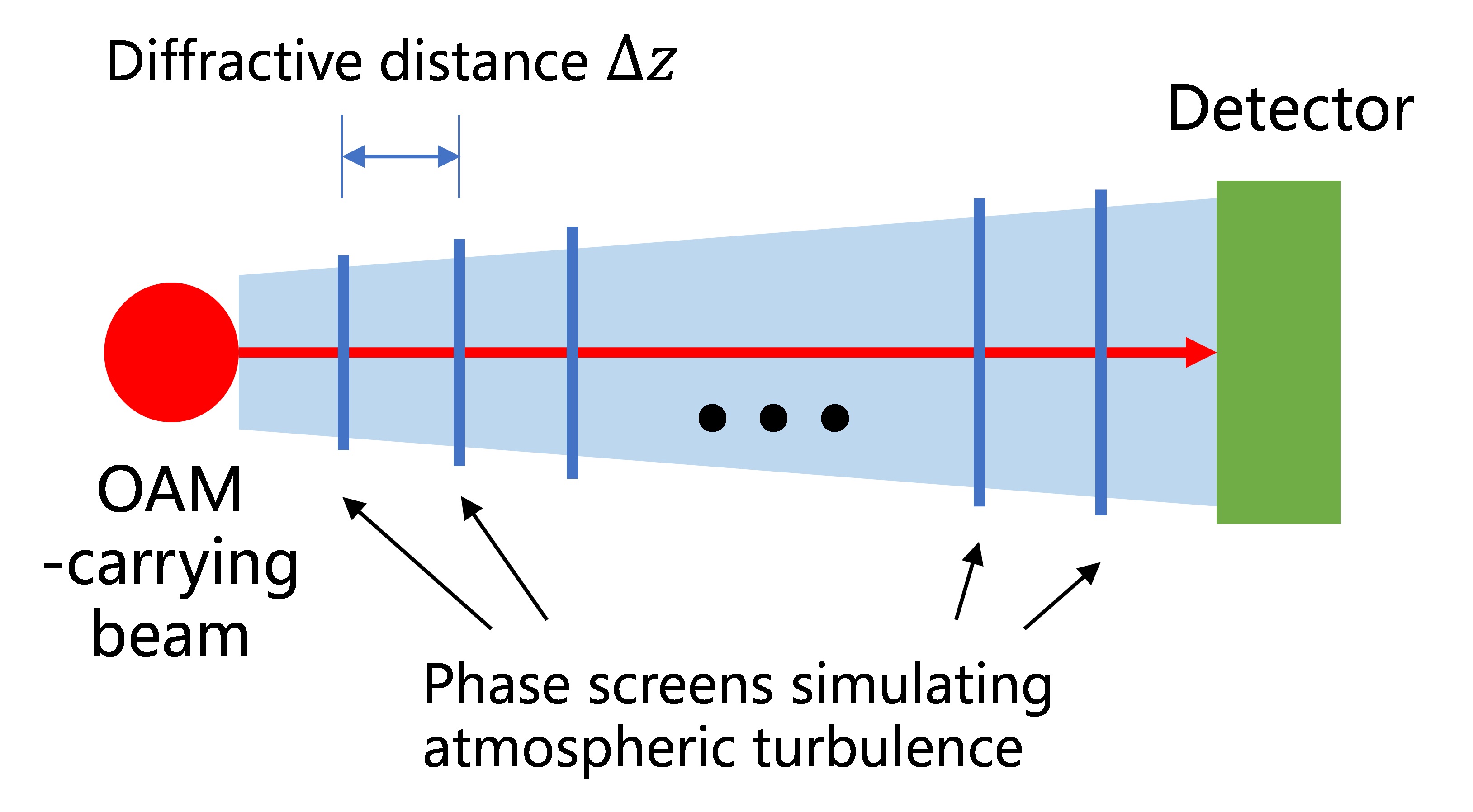
Figure 1: The source generates a single LG mode and sends it through a turbulent atmosphere (modeled by multiple turbulent cells arranged as ladder-shaped distribution) toward a detector. The phase-screen array is ladder-shaped distributed because the divergence angle of LG modes becomes larger with the increase of propagation distance while holding $w_{0}$ of the LG modes constant[41].

2 DESCRIPTION OF THE CROSSTALK EVOLUTION

The conceptual diagram of optical system that is simulated by our numerical procedure is shown in Fig. 1. Without loss of generality, we suppose that $z$ is the propagation distance, and the incident OAM-carrying beam is a single LG mode with azimuthal index $l_{0}$ and radial index $p_{0}$, which can be expressed in cylindrical coordinates by

$$LG_{p_{0},l_{0}}^{\left(q_{0}\right)}\left(r,\phi,0\right) =A\left(\frac{i\sqrt{kz_{R}}r}{q_{0}}\right)^{\left|l_{0}\right|+1}L_{p_{0}}^{\left|l_{0}\right|}\left(\frac{kz_{R}r^{2}}{\left|q_{0}\right|^{2}}\right)$$

$$\left(-\frac{q_{0}^{\ast}}{q_{0}}\right)^{p_{0}}\frac{e^{-\frac{ikr^{2}}{2q_{0}}}}{r}e^{il_{0}\phi},$$ (1)

with $L_{p_{0}}^{\left|l_{0}\right|}\left(\cdot\right)$ as the generalized Laguerre polynomial, where $A=\sqrt{p_{0}!/\pi\left(\left|l_{0}\right|+p_{0}\right)!}$ is the normalization constant and $q_{0}=iz_{R}$ represents the complex parameter associated with beam waist. $z_{R}=\pi w_{0}^{2}/\lambda$ and $k=2\pi/\lambda$ denote the Rayleigh range and the wave number respectively, $\lambda$ is the wavelength and $w_{0}$ is the beam waist at input plane.

Beam propagating through a turbulent channel is often described by the split-step beam propagation method[28]. It generally means that, as shown in Fig. 1, a turbulent channel can be divided into a series of turbulent cells, each cell introduces a random contribution $\phi$ to the phase, but essentially no change in the amplitude; besides, intensity fluctuations build up by diffraction over many cells. To agree well with the phase structure function of the Kolmogorov turbulence model, random phase screen lost low spatial frequencies need to be compensated using subharmonic method[42].

With this in mind, the split-step method is used to simulate the procedure of atmospheric propagation instead of the SPS approximation. Since LG modes with same $w_{0}$ form an orthonormal basis, the complex quantity $q_{0}$ is modified to $q\left(z\right)=z+q_{0}$ during the spectral decomposition for attributing the intermodal crosstalk to the impact of turbulence entirely, where the notation $q\left(z\right)$ called the Siegman complex parameter[43]. Hence, the received optical field can be decomposed into a superposition of several LG modes

$$U_{p,l}\left(r,\phi,z\right)=\sum_{p=0}^{\infty}\sum_{l=-\infty}^{\infty}c_{p,l}LG_{p,l}^{\left(q\right)}\left(r,\phi,z\right),$$ (2)

with the coefficient $c_{p,l}$ calculating from the overlap integral

$$c_{p,l}=\int_{0}^{\infty}rdr\int_{0}^{2\pi}d\phi U_{p,l}\left(r,\phi,z\right)LG_{p,l}^{\left(q\right)\ast}\left(r,\phi,z\right),$$ (3)

where the asterisk denotes the complex conjugate. Besides, the fraction of optical power that is transferred from the input mode with azimuthal index $l_{0}$ to other modes with azimuthal index $l$ can be described as

$$P\left(l\right)=\sum_{p=0}^{\infty}\left|c_{p,l}\right|^{2},$$ (4)

From the above analysis, we summary the effects of atmospheric turbulence on a LG mode with more intuitive way: the optical power of the input mode with azimuthal index $l_{0}$ is carved into unlimited pieces in terms of the power fraction $\left|c_{p,l}\right|^{2}$; each piece of LG modes attachs a turbulence-induced random phase in terms of the argument of the overlap intergral, namely, $\arg\left(c_{p,l}\right)$.

3 NUMERICAL REEXAMINATION OF THE IPE

3.1 Several parameters

To reexamine whether the minimal set of parameters obtained by the IPE remains valid to completely determine the crosstalk evolution considering the radial-mode scrambling, we briefly review several dimensionless quantities that are theoretically indispensable in the result of the IPE prediction: the normalized propagation distance $t\equiv z/z_{R}$, the normalized turbulence strength $K\equiv C_{n}^{2}w_{0}^{11/3}\pi^{3}/\lambda^{3}$ and the relative beam width $W\equiv w_{0}/r_{0}$, where $C_{n}^{2}$ is the refractive index structure constant, $r_{0}$ is the Fried parameter. Besides, the compound quantities $W$, $K$, and $t$ are related by[22, 38, 39]

$$W=1.37\left(Kt\right)^{3/5},$$ (5)

The intensity fluctuation of an optical field propagating through atmospheric turbulence is often centered around the scintillation index (For a more general expression of scintillation index, we refer the reader to Ref. [44]), which is the normalized variance of intensity fluctuation, and can be defined as[27]

$$\sigma_{I}^{2}\equiv\frac{\left\langle I^{2}\right\rangle-\left\langle I\right\rangle^{2}}{\left\langle I\right\rangle^{2}}=\frac{\left\langle I^{2}\right\rangle}{\left\langle I\right\rangle^{2}}-1,$$ (6)

where the notation $I$ and $\left\langle\cdot\right\rangle$ represent the intensity of an optical field and ensemble average, respectively. Under the weak scintillation condition based on the Kolmogorov turbulence model, the scintillation index of a plane wave can be expressed by[27, 45]

$$\sigma_{R}^{2}=1.23C_{n}^{2}k^{7/6}z^{11/6},$$ (7)

which can also be used to describe the intensity fluctuation over the turbulent link when extended to strong scintillation condition by increasing either $C_{n}^{2}$ or $z$, or both. The link between these two quantities is that under the weak scintillation condition, the scintillation index is proportional to the Rytov variance for a plane wave. In other words, the scintillation index increases with increasing values of the Rytov variance until it reaches a maximum value greater than unity in the regime characterized by random focusing[45]. Hence, we employ the Rytov variance as an indicator of the scintillation strength to avoid the circumstance that one scintillation index corresponds to two scintillation conditions. The Rytov variance can be also expressed in terms of $K$ and $t$[22, 39]

$$\sigma_{R}^{2}=1.64W^{5/3}t^{5/6}=1.055W^{55/18}/K^{5/6},$$ (8)

3.2 Data details and notes

The result of numerical simulation in one iteration, representing a single realization of turbulence, can be repeated several times. The ensemble average of different iterations of the two steps represents the result of crosstalk evolution under one fixed compound quantity (i.e., $K$ or $t$). Table 1 gives the different values of $K$ used in our simulation. For convenience of comparison, the turbulence strength $C_{n}^{2}$, the beam waist $w_{0}$, and the wavelength $\lambda$ are specifically assigned to guarantee that $W$ is limited to a certain range. Therefore, sampling intervals and propagation distances vary with the variation of $K$ in Table 1 during these simulations.

Eq. (8) gives the relationship between $\sigma_{R}^{2}$ and $K$. Hence, it can be observed that different scintillation conditions can be acquired during the numerical simulations by adjusting this compound quantity with fixed $W$. Further, since the spacing between two turbulent cells varies smartly with these parameters, different numbers of LG modes used for spectral decomposition are set in these simulations. Finally, it is worth highlighting that the total propagation distance ranges from a few meters to hundred kilometers.

3.3 Evolution rule under arbitrary scintillation conditions

The fraction of optical power obtained in the output plane that remains in the input LG mode (we call this as the eigen-crosstalk probability in this paper; (a1) $l_{0}=0$, (b1) $l_{0}=1$, (c1) $l_{0}=2$, (d1) $l_{0}=3$) is illustrated in Fig. 2. All plots are plotted as a function of $W$. Solid curve in all plots correspond to the results of the SPS model using quadratic approximation[46], while the results of our numerical results are shown with different shaped lines, corresponding to different values of $K$ given in Table 1. According to Eq. (8), the Rytov variances in $K=0.05$ are shown in all right-column plots with dashed lines. The dotted lines with small-spacing represent the deviation scale, while the large-spacing ones represent the scale determining the onset of strong scintillation. The horizontally dashed-dotted lines correspond to $\sigma_{R}^{2}=1$.

Table 1: Different values of the compound quantity $K$ composed of beam parameters and turbulence parameters shown in Fig. 2.

$K$	$C_{n}^{2}\left(m^{-2/3}\right)$	$w_{0}\left(m\right)$	$\lambda\left(nm\right)$
$0.05$	$10^{-16}$	$0.05$	$1000$
$0.1$	$10^{-16}$	$0.07$	$1214$
$0.3$	$10^{-16}$	$0.1$	$1314$
$0.8$	$5\times 10^{-16}$	$0.05$	$689$
$2$	$5\times 10^{-16}$	$0.08$	$900$
$5$	$5\times 10^{-15}$	$0.05$	$807$
$20$	$10^{-14}$	$0.05$	$640$
$100$	$10^{-13}$	$0.08$	$1432$
$1000$	$10^{-12}$	$0.08$	$1434$
$10^{4}$	$5\times 10^{-12}$	$0.1$	$1495$

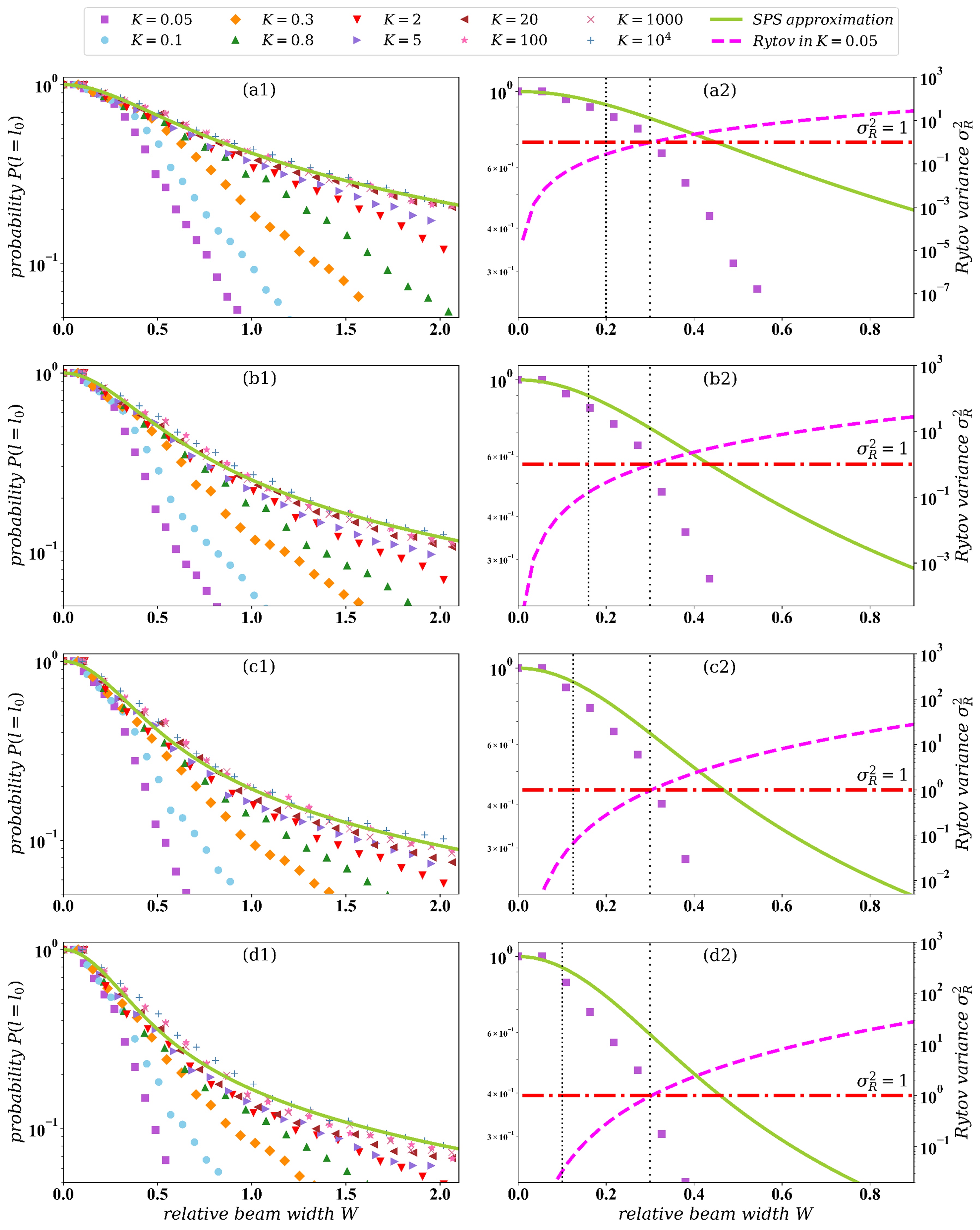
Figure 2: The eigen-crosstalk probabilities averaged over 300 realizations of turbulence as a function of $W$ under different values of normalized turbulence strengths $K$ given in Table 1 for (a1) $l_{0}=0$, (b1) $l_{0}=1$, (c1) $l_{0}=2$, (d1) $l_{0}=3$. The solid lines represent the results of the SPS approximation. The Rytov variances in $K=0.05$ (weak turbulence) are provided in the right-column plots. The short-spacing dotted lines and long-spacing dotted lines represent the deviation scale and the scale determining the onset of strong scintillation, respectively. For each azimuthal index $l_{0}$, the deviation scale appears at a smaller value compared to the scale determining the onset of strong scintillation. The horizontally dashed-dotted lines in all right-column plots correspond to $\sigma_{R}^{2}=1$. The solid line and the square scatter points in the right-column plots ((a2) $l_{0}=0$; (b2) $l_{0}=1$; (c2) $l_{0}=2$; (d2) $l_{0}=3$) is the partial enlargement of the results presented in the left-column plots.

We observe that for large values of $K$ (e.g., $K\gtrsim 20$ for $l_{0}=0,1$ and $K\gtrsim 100$ for $l_{0}=2,3$), the evolution curves of the eigen-crosstalk probability obtained by our numerical simulation almost coincide with the result of the SPS approximation. However, this coincidence does not exist as $K$ becomes smaller (e.g., $K\lesssim 5$ for $l_{0}=0,1$ and $K\lesssim 20$ for $l_{0}=2,3$), which means that another compound quantity $K$ is needed to be added to describe the evolution of eigen-crosstalk probability except $W$. Moreover, we found that the eigen-crosstalk probability of input modes with a larger azimuthal index ($l_{0}\gtrsim 2$) decreases faster compared to that of the smaller one, more obviously when $K\lesssim 2$, which is likely because LG modes with a larger $l_{0}$ possess a larger beam waist so that it’s more susceptible to atmospheric turbulence.

The deviation phenomenon between the results of numerical simulation and that of the SPS approximation under arbitrary turbulence strengths is also shown in Fig. 2. We zoom in the results of numerical simulation of $K=0.05$ in the right-column of Fig. 2 ((a2) $l_{0}=0$, (b2) $l_{0}=1$, (c2) $l_{0}=2$, (d2) $l_{0}=3$). The crossing points of the numerical curves and the large-spacing dotted lines represent the onset of strong scintillation, while the crossing points of the numerical curves and the short-spacing dotted lines indicate at what values of the Rytov variance the deviation occur. Notably, the results in Fig. 2 seem to indicate that LG modes with a larger azimuthal index have a smaller deviation scale. Further, it reveals a well-known conclusion that the deviation scale is always smaller than the scale determining the onset of strong scintillation[22]. However, why are they different? more straightforwardly, what is the nature of the deviation scale? It deserves to be investigated, and it is also the topic of this paper.

3.4 Verification of the minimal set of parameters

The evolution curves of eigen-crosstalk probability as a function of $W$ for $l_{0}=0$ are illustrated in Fig. 3. These curves are obtained in $K=0.066$ with different combinations of dimension parameters shown in Table 2. The smaller $K$ is chosen because it represents a condition where the evolution of eigen-crosstalk probability deviates significantly from that of the SPS approximation[38]. We observe that although different sets of parameters are selected in the numerical simulation, all of curves coincide under the same $K$, which means all kinds of beam parameters and turbulence parameters (i.e., $C_{n}^{2}$, $z$, $w_{0}$ and $\lambda$) always appear in the form of compound quantities (i.e., $K$, $t$, and $W$) within the crosstalk evolution calculated by the Kolmogorov turbulence model under arbitrary scintillation conditions. Compared to the minimal set of parameters that decides the result of the IPE prediction, one can conclude that these parameters remain valid to completely determine the crosstalk evolution considering the radial-mode scrambling.

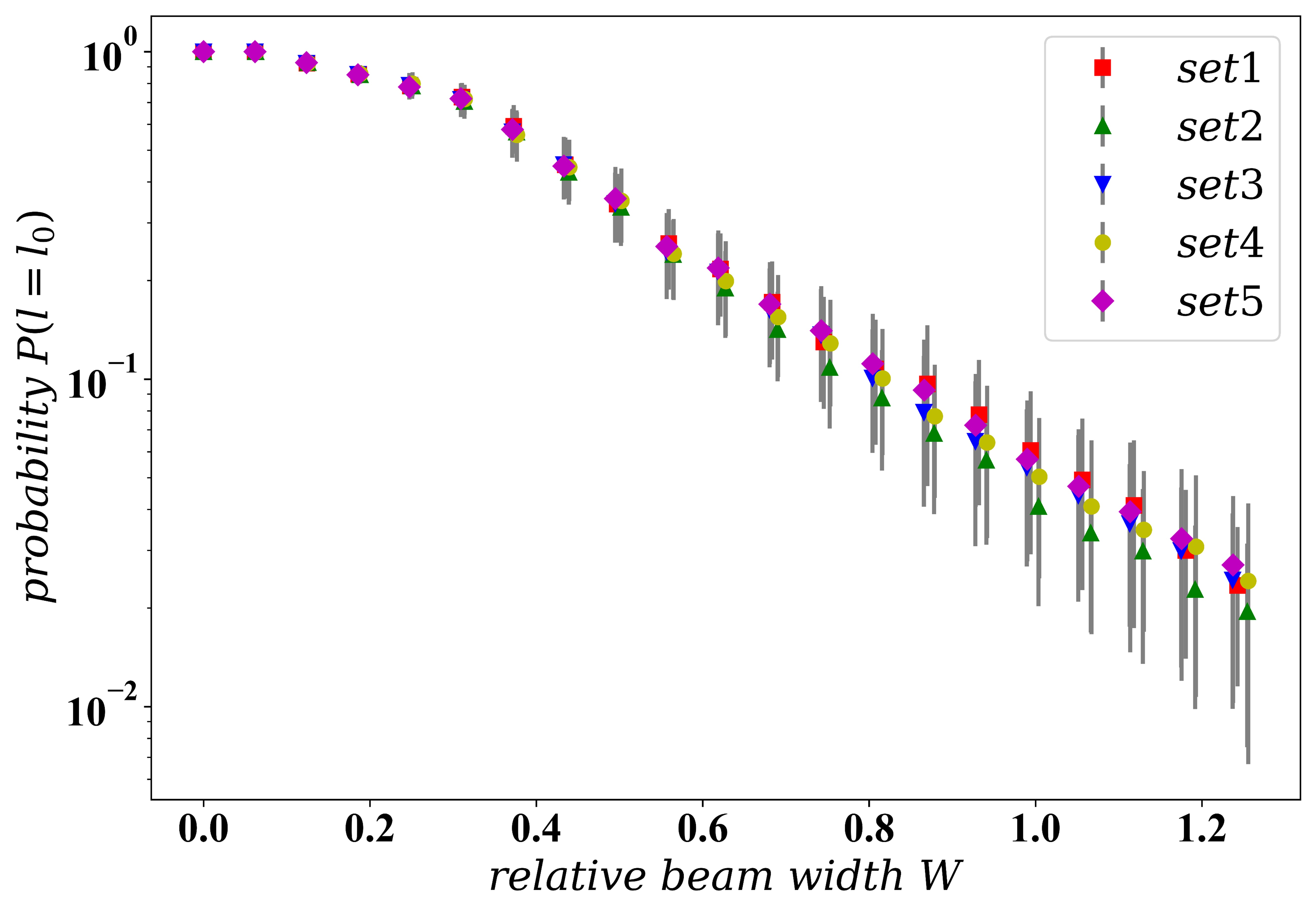
Figure 3: The eigen-crosstalk probability as a function of $W$ with the same normalized turbulence strength $K=0.066$ given in Table 2 for $l_{0}=0$, averaged over 300 realizations of turbulence. Each set of dimensionless parameters are combined with different beam and turbulence parameters. The error bars represent the standard error.

Table 2: Different combinations of beam parameters and turbulence parameters for $K=0.066$ shown in Fig. 3.

$set$	$C_{n}^{2}\left(m^{-2/3}\right)$	$w_{0}\left(m\right)$	$\lambda\left(nm\right)$
$1$	$10^{-17}$	$0.1$	$1000$
$2$	$10^{-16}$	$0.05$	$924$
$3$	$5\times 10^{-18}$	$0.1$	$794$
$4$	$5\times 10^{-17}$	$0.08$	$1302$
$5$	$10^{-18}$	$0.13$	$640$

Table 3: Different values of the compound quantity $t$ composed of beam parameters and turbulence parameters shown in Fig. 4.

$t$	$z\left(km\right)$	$w_{0}\left(m\right)$	$\lambda\left(nm\right)$
$2\times 10^{-4}$	$5\times 10^{-3}$	$0.1$	$1263$
$10^{-3}$	$3\times 10^{-2}$	$0.08$	$672$
$10^{-2}$	$0.1$	$0.06$	$1169$
$0.1$	$1.2$	$0.05$	$658$
$0.5$	$5$	$0.05$	$791$
$1$	$22.5$	$0.08$	$900$
$1.5$	$30$	$0.07$	$770$
$2$	$50$	$0.08$	$806$
$3$	$70$	$0.08$	$864$
$5$	$100$	$0.08$	$1000$
$10$	$200$	$0.08$	$1000$

4 PHYSICAL MEANING OF THE DEVIATION SCALE

4.1 Qualitative understanding

From above analysis, we highlight that compound quantities composed of $K$ and $W$ can completely determine the crosstalk evolution caused by atmospheric turbulence. Consequently, it not necessarily investigates the crosstalk evolution under different values of normalized propagation distance $t$. However, although $K$, $t$ and $W$ are pairwise independent compound quantities, it may be help us to give a qualitative understanding of the deviation scale by studying the influence of $t$ on the eigen-crosstalk probability.

To better determine the value of $\sigma_{R}^{2}$ and $t$ where the results of the IPE prediction (we believe the results of numerical simulation are equivalent to that of the IPE prediction due to the validity of the minimal set of parameters) start to deviate from that of the SPS approximation, in Fig. 4 we illustrate how the difference of eigen-crosstalk probability between these two results, namely, $\Delta P\equiv P_{SPS}-P_{IPE}$, changes with respect to $\sigma_{R}^{2}$ under different values of $t$ shown in Table 3. For convenience of analysis, Fig. 4 is divided into four areas. We see that the points where the IPE predictions start to deviate from the SPS counterparts occur at $\sigma_{R}^{2}\simeq 0.1$, especially for the larger value of $t$. Further, we observe that when $0.1<\sigma_{R}^{2}<1$ and $t<0.5$, the deviation between these two results remains still very small. On the contrary, if the above conditions do not hold any more, the deviation will grow rapidly with the increase of $\sigma_{R}^{2}$ even if the turbulent channel is still under the weak scintillation condition.

We mark a series of cruciform scatter points in Fig. 4, which represents the results obtained in $K=0.05$. Based on these results, we can observe clearly why the deviation always appears at smaller values than the scale determining the onset of strong scintillation. That is because the difference of eigen-crosstalk probability in $K=0.05$ have exceeded the above threshold of $t$ in the regime of $0.1<\sigma_{R}^{2}<1.$ Actually, this effect can be seen more clearly when Fig. 2 is plotted as a function of $t$ instead of $W$. Hence, we can qualitatively conclude that the SPS approximation is valid if $\sigma_{R}^{2}<1$ and $t<0.5$ for LG modes.

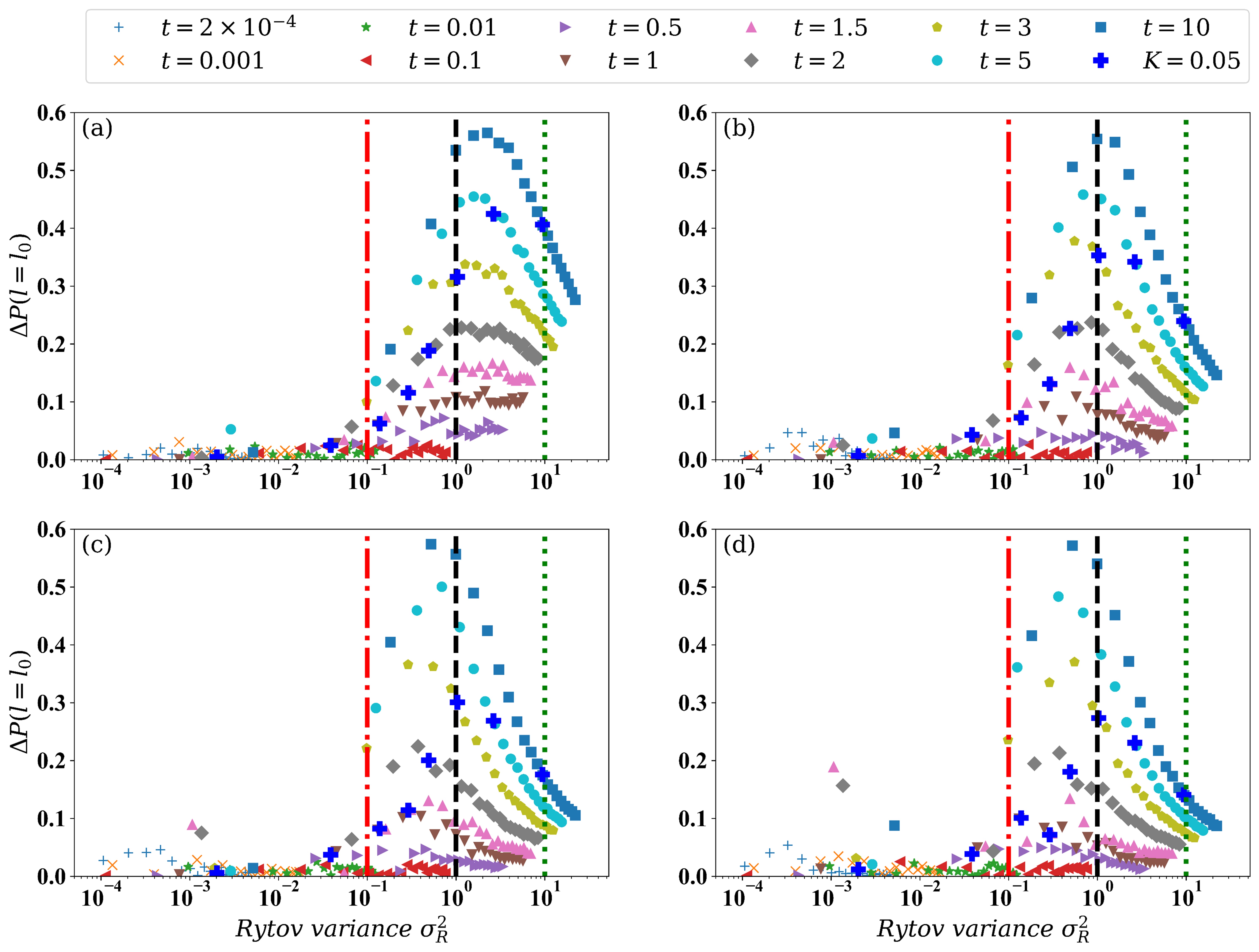
Figure 4: The difference curves of eigen-crosstalk probability between the results of the IPE prediction and that of the SPS approximation, namely, $\Delta P\equiv P_{SPS}-P_{IPE}$, averaged over 300 realizations of turbulence as a function of $\sigma_{R}^{2}$ under different normalized propagation distances $t$ given in Table 3 for (a) $l_{0}=0$, (b) $l_{0}=1$, (c) $l_{0}=2$, (d) $l_{0}=3$. Each graph is divided by four areas composed of $\sigma_{R}^{2}<0.1$, $0.1<\sigma_{R}^{2}<1$, $1<\sigma_{R}^{2}<10$ and $\sigma_{R}^{2}>10$. A series of cruciform scatter points are marked, representing the results obtained in $K=0.05$.

Other than the interrogation of the nature of the deviation scale, we can also conclude some other interesting phenomena from the results in Fig. 4, which can be summarized as follows: When the scintillation condition is beyond the weak range (i.e., $1<\sigma_{R}^{2}<10$), the deviation between two results becomes smaller as the increase of $\sigma_{R}^{2}$. When $\sigma_{R}^{2}>10$, these deviations together incline to disappear, which is likely because of the effect of scintillation saturation.

4.2 Quantitative understanding

What can be seen from the above analysis is that the deviation between the results of the IPE prediction and that of the SPS approximation comes from the spatial accumulation of the intensity modulation of the input LG mode. In other words, for a LG mode that are perturbed while propagating over a series of turbulent cells the compound effect on the LG mode is more damaging than the effect of simply accumulating the phase perturbation over the link. The direct result of the intensity modulation changes the location of the original vortex. Hence, we anticipate that even if the turbulent channel is under the weak scintillation condition, the spatial accumulation of slight intensity modulation of the input LG mode splits the vortex into multiple individual vortices with a TC of $+1$ and re-generates the vortex-antivortex pairs with a TC of $+1$ and with a TC of $-1$, which may be the main reason for the appearance of the deviation scale.

To examine our anticipation, Fig. 5 illustrates the evolution curves of the eigen-crosstalk probability, the average OAM and vortex-splitting ratio[20, 21] in the output plane, all of which are calculated under $K=0.05$ and different values of $l_{0}$. Besides, all plots are plotted as a function of $W$. Notably, the reason why we choose the vortex-splitting ratio as an indicator to examine our anticipation is that for LG modes with a specific azimuthal index, this parameter contains much information about the vortex distribution in the phase of the received optical field, which characterizes all the effects of atmospheric propagation under the weak scintillation condition. Considering atmospheric turbulence can also generate vortex-antivortex pairs, the vortex-splitting ratio can be re-evaluated by[36]

$$\nu\equiv\frac{1}{Nw_{0}}{\displaystyle\sum\limits_{i=1}^{N}}q_{i}V_{r}^{\left(i\right)}.$$ (9)

where $N$ represents the total number of vortices in the output plane. Each vortex is identified by the index $i$. $q_{i}$ and $V_{r}^{\left(i\right)}$ stand for the TC of the vortex with index $i$ and the radial distance from the beam origin for the vortex with index $i$, respectively. We have to emphasize that this definition not only takes account into the turbulence-induced vortex-antivortex pairs but also includes the effect of vortex-splitting. Our vortex detection algorithm is a modified version of the algorithm proposed in Refs. [47, 48, 49, 50].

Figure 5: The eigen-crosstalk probabilities ((a)–(c)), the vortex-splitting ratio and the average OAM ((d)–(f)), averaged over 300 realizations of turbulence as a function of $W$ with $K=0.05$: (a), (d) $l_{0}=1$, (b), (e) $l_{0}=2$, (c), (f) $l_{0}=3$. The standard errors are plotted by the shaded area around each curve. The solid lines represent the results of the SPS approximation. The Rytov variance in $K=0.05$ are depicted in dashed line. (a)–(c) are horizontally divided into two areas composed of $\sigma_{R}^{2}<1$ and $\sigma_{R}^{2}>1$ using dashed-dotted lines. The splitting-thresholds that represent the appearance of the deviation scale for different azimuthal indices of LG modes are plotted by the dotted line in (d)–(f): (d) $\nu=0.1$ for $l_{0}=1$, (e) $\nu=0.15$ for $l_{0}=2$, (f) $\nu=0.2$ for $l_{0}=3$. These splitting-thresholds can be easily translated into the threshold of $t$ with different values: (d) $t=0.648$ for $l_{0}=1$, (e) $t=0.369$ for $l_{0}=2$, (f) $t=0.255$ for $l_{0}=3$.

We observe in Fig. 5 that for different azimuthal indices of LG modes and specific turbulence strength, the phenomena of vortex splitting and vortex-antivortex pairs re-generation occur in the output plane at the early stages of propagation (e.g., for $l_{0}=1$, atmospheric turbulence steers the original vortex off beam axis and leads to the vortex-antivortex pairs re-generation). Other than that, we see that the compound effect caused by atmospheric turbulence, quantified by the vortex-splitting ratio, becomes more pronounced progressively as $W$ increases. This behavior can be seen more clearly when the curves are plotted as a function of $t$ instead of $W$. Based on the results presented in Fig. 5, we found that with the increase of the vortex splitting ratio (e.g., $\nu\geq 0.1$ for $l_{0}=1$, $\nu\geq 0.15$ for $l_{0}=2$ and $\nu\geq 0.2$ for $l_{0}=3$), the average OAM and the eigen-crosstalk probabilities gradually deviate from the results of the SPS approximation. A suitable explanation is that when the turbulent channel is under the weak scintillation condition, the turbulence-induced intensity fluctuation splits the original vortex into multiple vortices with a TC of $+1$ in the output plane, and possibly accompanied by the re-generation of vortex-antivortex pairs that carry opposite-sign unity TC. After undergoing the spatial accumulation of a considerable amount of compound effect, the probability of detecting the TC of $+1$ in the phase distribution of the received optical field becomes more larger, which leads to a significant reduction of the average OAM and the deviation between the results of the IPE prediction and that of the SPS approximation.

Therefore, we believe the appearance of the deviation is actually the process of the spatial accumulation of the compound effect. From the results presented in Fig. 5 (see the rectangular shaded areas in all six plots), it is worth highlighting that such phenomena will happen only if the vortex-splitting ratio of the received optical field is beyond a specific threshold (we call this as the splitting-threshold, e.g., $\nu=0.1$ for $l_{0}=1$, $\nu=0.15$ for $l_{0}=2$ and $\nu=0.2$ for $l_{0}=3$). Other than that, it is not difficult to find that different splitting-thresholds that we obtained in fact provide a more precise application scope of the SPS approximation for LG modes with a specific azimuthal index. To this end, we calculate the values of normalized propagation distance $t$ that correspond to the aforementioned splitting-thresholds by Eq. (5), namely, $t=0.648$ for $l_{0}=1$, $t=0.369$ for $l_{0}=2$ and $t=0.255$ for $l_{0}=3$. The reason why $t$ becomes smaller as $l_{0}$ increases is that LG modes with a larger azimuthal index possess a larger beam waist so that it’s more susceptible to atmospheric turbulence.

On the other hand, we also verify our anticipation in Fig. 6 with a more straightforward way, which is a evident illustration of the phase distributions of the received optical field. The OAM spectra of the received optical field, averaged over 300 realizations of turbulence under the weak scintillation condition, are also plotted in Fig. 6. The top row in Fig. 6 represents the results below the splitting-threshold (e.g., (a) $\nu=0.0337$, (b) $\nu=0.1112$, (c) $\nu=0.1968$, corresponding to $t=0.157$ approximately), while the bottom row represents the results above the splitting-threshold (e.g., (d) $\nu=0.2603$, (e) $\nu=0.4447$, (f) $\nu=0.599$, corresponding to $t=1.376$ approximately). By comparing the results between top and bottom, we also obtain the same conclusions presented in Fig. 5, which is exactly the kind of result we expected. More importantly, we observe in the top row of Fig. 6 that a pair of vortex-antivortex pairs occurs in the phase distribution of the received optical field even when the vortex-splitting ratio is below the splitting-threshold (see Fig. 6(c)), which makes us more confident to the above physical interpretation of the deviation scale.

At last, we conclude that the appearance of deviation scale cannot be predicted only by the Rytov variance, which can be predicted through the vortex-splitting ratio of the received optical field alone or with the help of $t$. In other words, it is not completely scientific for us to employ the SPS approximation to simulate the crosstalk evolution of atmospheric propagation even when the turbulent channel is under the weak scintillation condition.

Figure 6: OAM spectra averaged over 300 realizations of turbulence and phase distributions of the received optical field for a single realization of turbulence with different azimuthal indices: (a), (d) $l_{0}=1$, (b), (e) $l_{0}=2$, (c), (f) $l_{0}=3$. The top row represents the results below the splitting-thresholds ((a) $\nu=0.0337$; (b) $\nu=0.1112$; (c) $\nu=0.1968$), corresponding to $t=0.157$ approximately. The bottom row represents the results above the splitting-thresholds ((d) $\nu=0.2603$; (e) $\nu=0.4447$; (f) $\nu=0.599$), corresponding to $t=1.376$ approximately. The colorbar for all phase distributions (a)–(f) are the same. The dashed lines denote the eigen-crosstalk probabilities obtained from the results of the SPS approximation and the arrows point to the eigen-crosstalk probabilities obtained from the results of the IPE prediction. The bi-color dots (i.e., black dots and white dots) plotted in each partial enlarged plot indicate the location of individual vortices, corresponding to a TC of $+1$ and a TC of $-1$, respectively.

5 CONCLUSION

In this paper, we give a suitable physical interpretation for the recently so-called deviation scale [C. M. Mabena et al., Phys. Rev. A 99, 013828 (2019)], which bridges the connection between the result of the IPE prediction and that of the SPS approximation. Before we explain the nature of the deviation scale, we reexamine whether the minimal set of parameters obtained by the IPE remains valid to completely determine the crosstalk evolution considering the radial-mode scrambling. The process of re-examination extends the results of the IPE and proofs the validity of our numerical simulation. In our endeavor to present a qualitative understanding of the deviation scale, we found that when the scintillation condition, measured by the Rytov variance, is weak, namely, $\sigma_{R}^{2}<1$ and the normalized propagation distance is below than a specific threshold, namely, $t<0.5$, the evolution curve of eigen-crosstalk probability almost coincides with that of the SPS approximation. However, when $t>0.5$, the deviation scale starts to appear and becomes larger as $\sigma_{R}^{2}$ increases, which qualitatively gives a rough application scope of the SPS approximation for an OAM-carrying beam propagating through atmospheric turbulence. Furthermore, we demonstrate what the deviation scale actually represents from some quantitative calculation. Our quantitative understanding is that the spatial accumulation of slight intensity modulation of the incident OAM-carrying beam splits the original vortex into multiple individual vortices with a TC of $+1$ and re-generates the vortex-antivortex pairs with a TC of $+1$ and with a TC of $-1$, leading to a significant reduction of the value of the average OAM in the output plane and the deviation between the results of the IPE prediction and that of the SPS approximation. Notably, such phenomena will happen only if the disruption of this compound effect on the phase distribution of the incident OAM-carrying beam becomes more significant, which can be quantified by vortex-splitting ratio of the received optical field. Or to put in another way, such phenomena will happen only if the vortex-splitting ratio is beyond the splitting-threshold (e.g., $\nu=0.1$ for $l_{0}=1$, $\nu=0.15$ for $l_{0}=2$ and $\nu=0.2$ for $l_{0}=3$). In fact, the aforementioned two interpretations are equivalent because the qualitative description gives a complete parameter condition (i.e., $\sigma_{R}^{2}$ and $t$) composed of beam parameters and turbulence parameters (i.e., $C_{n}^{2}$, $z$, $w_{0}$ and $\lambda$) to determine the appearance of the deviation scale, while the quantitative one is obtained from the splitting-threshold condition that completely and comprehensively evaluates the results of the compound effect in the output plane, which can be easily translated into the threshold of $t$ with different values (e.g., $t=0.648$ for $l_{0}=1$; $t=0.369$ for $l_{0}=2$; $t=0.255$ for $l_{0}=3$). Generally, the quantitative calculation offers a more precise application scope of the SPS approximation. On the other hand, these conclusions also reveal that the appearance of deviation scale cannot be predicted only by the Rytov variance, which can be measured with the help of $t$ or predicted through the vortex-splitting ratio of the received optical field alone.

Funding. Anhui Provincial Natural Science Foundation (1908085QA37); National Natural Science Foundation of China (11904369); State Key Laboratory of Pulsed Power Laser Technology Supported by Open Research Fund of State Key Laboratory of Pulsed Power Laser Technology (2019ZR07).

Acknowledgment. We would like to thank the anonymous reviewers for their valuable comments, which significantly improves the presentation of this paper. We acknowledge the helpful discussion with Professor Filippus Stef Roux. Zhiwei Tao thanks Professor Ruizhong Rao for his insightful suggestions.

Disclosures. The authors declare no conflicts of interest.

References

- [1] L. Allen, M. W. Beijersbergen, R. J. C. Spreeuw, and J. P. Woerdman, "Orbital angular momentum of light and the transformation of Laguerre-Gaussian laser modes," Phys. Rev. A 45, 8185–8189 (1992).
- [2] M. A. Cox, L. Cheng, C. Rosales-Guzmán, and A. Forbes, "Modal diversity for robust free-space optical communications," Phys. Rev. Applied 10, 024020 (2018).
- [3] M. P. MacDonald, L. Paterson, K. Volke-Sepulveda, J. Arlt, W. Sibbett, and K. Dholakia, "Creation and manipulation of three-dimensional optically trapped structures," Science 296, 1101–1103 (2002).
- [4] A. Jesacher, S. Fürhapter, S. Bernet, and M. Ritsch-Marte, "Size selective trapping with optical “cogwheel” tweezers," Opt. Express 12, 4129–4135 (2004).
- [5] L. Torner, J. P. Torres, and S. Carrasco, "Digital spiral imaging," Opt. Express 13, 873–881 (2005).
- [6] L. Chen, J. Lei, and J. Romero, "Quantum digital spiral imaging," Light Sci. Appl. 3, e153 (2014).
- [7] M. P. J. Lavery, F. C. Speirits, S. M. Barnett, and M. J. Padgett, "Detection of a spinning object using light’s orbital angular momentum," Science 341, 537–540 (2013).
- [8] A. Mair, A. Vaziri, G. Weihs, and A. Zeilinger, "Entanglement of the orbital angular momentum states of photons," Nature 412, 313–316 (2001).
- [9] R. Fickler, R. Lapkiewicz, M. Huber, M. P. J. Lavery, M. J. Padgett, and A. Zeilinger, "Interface between path and orbital angular momentum entanglement for high-dimensional photonic quantum information," Nat. Commun. 5, 4502 (2014).
- [10] M. Malik, M. Mirhosseini, M. P. J. Lavery, J. Leach, M. J. Padgett, and R. W. Boyd, "Direct measurement of a 27-dimensional orbital-angular-momentum state vector," Nat. Commun. 5, 3115 (2014).
- [11] C. Paterson, "Atmospheric turbulence and orbital angular momentum of single photons for optical communication," Phys. Rev. Lett. 94, 153901 (2005).
- [12] G. A. Tyler and R. W. Boyd, "Influence of atmospheric turbulence on the propagation of quantum states of light carrying orbital angular momentum," Opt. Lett. 34, 142–144 (2009).
- [13] J. R. G. Alonso and T. A. Brun, "Protecting orbital-angular-momentum photons from decoherence in a turbulent atmosphere," Phys. Rev. A 88, 022326 (2013).
- [14] Y. Zhang, I. B. Djordjevic, and X. Gao, "On the quantum-channel capacity for orbital angular momentum-based free-space optical communications," Opt. Lett. 37, 3267–3269 (2012).
- [15] C. Chen, H. Yang, S. Tong, and Y. Lou, "Changes in orbital-angular-momentum modes of a propagated vortex Gaussian beam through weak-to-strong atmospheric turbulence," Opt. Express 24, 6959–6975 (2016).
- [16] Y. Ren, H. Huang, G. Xie, N. Ahmed, Y. Yan, B. I. Erkmen, N. Chandrasekaran, M. P. J. Lavery, N. K. Steinhoff, M. Tur, S. Dolinar, M. Neifeld, M. J. Padgett, R. W. Boyd, J. H. Shapiro, and A. E. Willner, "Atmospheric turbulence effects on the performance of a free space optical link employing orbital angular momentum multiplexing," Opt. Lett. 38, 4062–4065 (2013).
- [17] M. Malik, M. O’Sullivan, B. Rodenburg, M. Mirhosseini, J. Leach, M. P. J. Lavery, M. J. Padgett, and R. W. Boyd, "Influence of atmospheric turbulence on optical communications using orbital angular momentum for encoding," Opt. Express 20, 13195–13200 (2012).
- [18] B. Rodenburg, M. Mirhosseini, M. Malik, O. S. Magaña-Loaiza, M. Yanakas, L. Maher, N. K. Steinhoff, G. A. Tyler and R. W. Boyd, "Simulating thick atmospheric turbulence in the lab with application to orbital angular momentum communication," New J. Phys. 16, 033020 (2014).
- [19] B. Rodenburg, M. P. J. Lavery, M. Malik, M. N. O’Sullivan, M. Mirhosseini, D. J. Robertson, M. Padgett, and R. W. Boyd, "Influence of atmospheric turbulence on states of light carrying orbital angular momentum," Opt. Lett. 37, 3537–3539 (2012).
- [20] M. P. J. Lavery, C. Peuntinger, K. Günthner, P. Banzer, D. Elser, R. W. Boyd, M. J. Padgett, C. Marquardt, and G. Leuchs, "Free-space propagation of high-dimensional structured optical fields in an urban environment," Sci. Adv. 3(10), e1700552 (2017).
- [21] M. P. J. Lavery, "Vortex instability in turbulent free-space propagation," New J. Phys. 20, 043023 (2018).
- [22] C. M. Mabena and F. S. Roux, "Optical orbital angular momentum under strong scintillation," Phys. Rev. A 99, 013828 (2019).
- [23] F. S. Roux, "Infinitesimal-propagation equation for decoherence of an orbital-angular-momentum-entangled biphoton state in atmospheric turbulence," Phys. Rev. A 83, 053822 (2011).
- [24] F. S. Roux, "Erratum: Infinitesimal-propagation equation for decoherence of an orbital-angular-momentum-entangled biphoton state in atmospheric turbulence [Phys. Rev. A 83, 053822 (2011)]," Phys. Rev. A 88, 049906(E) (2013).
- [25] F. S. Roux, "The Lindblad equation for the decay of entanglement due to atmospheric scintillation," J. Phys. A: Math. Gen. 47, 195302 (2014).
- [26] F. S Roux, "Non-Markovian evolution of photonic quantum states in atmospheric turbulence," J. Opt. 18, 055203 (2016).
- [27] L. C. Andrews and R. L. Phillips, Laser Beam Propagation through Random Media, 2nd ed. (SPIE, 2005).
- [28] J. D. Schmidt, Numerical Simulation of Optical Wave Propagation with Examples in Matlab (SPIE, 2010).
- [29] It is worth noting that the link between TC and OAM is only valid for rotationally symmetric beams, such as Laguerre-Gaussian modes and Bessel-Gaussian modes, to name just a few. In all other cases, the OAM in the beam is in general not proportional to the TC in the beam. The listed rotationally symmetric beams carry the same OAM normalized to the optical power, which is equal to the beams’ integer TC. For the latest progresses about TC, we refer the reader to Refs. [30, 31, 32, 33].
- [30] V. V. Kotlyar, A. A. Kovalev, and A. V. Volyar, "Topological charge of a linear combination of optical vortices: topological competition," Opt. Express 28, 8266–8281 (2020).
- [31] V. V. Kotlyar and A. A. Kovalev, "Topological charge of asymmetric optical vortices," Opt. Express 28, 20449–20460 (2020).
- [32] V. V. Kotlyar, A. A. Kovalev, A. G. Nalimov, and A. P. Porfirev, "Evolution of an optical vortex with an initial fractional topological charge," Phys. Rev. A 102, 023516 (2020).
- [33] A. A. Kovalev, V. V. Kotlyar, and A. P. Porfirev, "Orbital angular momentum and topological charge of a multi-vortex Gaussian beam," J. Opt. Soc. Am. A 37, 1740–1747 (2020).
- [34] X. L. Ge, B. Y. Wang, and C. S. Guo, "Evolution of phase singularities of vortex beams propagating in atmospheric turbulence," J. Opt. Soc. Am. A 32, 837–842 (2015).
- [35] G. Gbur and R. K. Tyson, "Vortex beam propagation through atmospheric turbulence and topological charge conservation," J. Opt. Soc. Am. A 25, 225–230 (2008).
- [36] G. Sorelli, V. N. Shatokhin, and A. Buchleitner, "Photonic orbital angular momentum in turbulence: vortex splitting and adaptive optics," Proc. SPIE 11532, 115320E (2020).
- [37] A. H. Ibrahim, F. S. Roux, M. McLaren, T. Konrad, and A. Forbes, "Orbital-angular-momentum entanglement in turbulence," Phys. Rev. A 88, 012312 (2013).
- [38] A. H. Ibrahim, F. S. Roux, and T. Konrad, "Parameter dependence in the atmospheric decoherence of modally entangled photon pairs," Phys. Rev. A 90, 052115 (2014).
- [39] F. S. Roux, "Entanglement evolution of twisted photons in strong atmospheric turbulence," Phys. Rev. A 92, 012326 (2015).
- [40] F. S. Roux, "Biphoton states in correlated turbulence," Phys. Rev. A 95, 023809 (2016).
- [41] M. J. Padgett, F. M. Miatto, M. P. J. Lavery, A. Zeilinger, and R. W. Boyd, "Divergence of an orbital-angularmomentum-carrying beam upon propagation," New J. Phys. 17, 023011 (2015).
- [42] G. Sedmak, "Implementation of fast-Fourier-transform-based simulations of extra-large atmospheric phase and scintillation screens," Appl. Opt. 43, 4527–4538 (2004).
- [43] G. Vallone, "Role of beam waist in Laguerre–Gauss expansion of vortex beams," Opt. Lett. 42, 1097–1100 (2017).
- [44] R. Rao, "General optical scintillation in turbulent atmosphere," Chin. Opt. Lett. 6, 547–549 (2008).
- [45] L. C. Andrews, R. L. Phillips, and C. Y. Young, Laser Beam Scintillation with Applications (SPIE, 2001).
- [46] J. C. Leader, "Atmospheric propagation of partially coherent radiation," J. Opt. Soc. Am. A 68, 175-185 (1978).
- [47] A. Dipankar, R. Marchiano, and P. Sagaut, "Trajectory of an optical vortex in atmospheric turbulence," Phys. Rev. E 80, 046609 (2009).
- [48] J. Borchardt, M. Duparre, and S. Skupin, "Tracking phase singularities in optical fields," Proc. SPIE 8274, 827410 (2012).
- [49] D. J. Sanchez and D. W. Oesch, "Orbital angular momentum in optical waves propagating through distributed turbulence," Opt. Express 24, 24596–24608 (2011).
- [50] D. W. Oesch, D. J. Sanchez, and C. M. Tewksbury-Christle, "Aggregate behavior of branch points - persistent pairs," Opt. Express 20, 1046–1059 (2012).