Tracking the orbit of unresolved subhalos for semi-analytic models

Abstract

We present a model to track the orbital evolution of “unresolved subhaloes” (USHs) in cosmological simulations. USHs are subhaloes that are no longer distinguished by halo finders as self-bound overdensities within their larger host system due to limited mass resolution. These subhaloes would host “orphan galaxies” in semi-analytic models of galaxy formation and evolution (SAMs). Predicting the evolution of the phase-space components of USHs is crucial for the adequate modelling of environmental processes, interactions and mergers implemented in SAMs that affect the baryonic properties of orphan satellites. Our model takes into account dynamical friction drag, mass loss by tidal stripping and merger with the host halo, involving three free parameters. To calibrate this model, we consider two DM-only simulations of different mass resolution (MultiDark simulations). The simulation with higher-mass resolution (smdpl; $m_{\rm DM}=9.6\times 10^{7}~{}h^{-1}\,\mathrm{M_{\odot}}$) provides information about subhaloes that are not resolved in the lower-mass resolution one (mdpl2; $m_{\rm DM}=1.5\times 10^{9}~{}h^{-1}\,\mathrm{M_{\odot}}$); the orbit of those USHs is tracked by our model. We use as constraining functions the subhalo mass function (SHMF) and the two-point correlation function (2PCF) obtained from smdpl, being the latter a novel aspect of our approach. While the SHMF fails to put tight constraints on the efficiency of dynamical friction and the merger condition, the addition of clustering information helps to specify the parameters of the model related to the spatial distribution of subhaloes. Our model allows to achieve good convergence between the results of simulations of different mass resolution, with a precision better than 10 per cent for both SHMF and 2PCF.

1 Introduction

The observed Universe is successfully described by the $\Lambda$CDM model. According to this concordance model, at early times, the Universe underwent a period of exponential expansion, called Inflation, in which the primordial perturbations in the metric were settled. These metric fluctuations produced perturbations in the matter density field that are characterised by the matter power spectrum. The large scale structure (LSS) we see today is the result of the gravitational growth of these tiny matter perturbations. It is currently accepted that structure formation proceeds in a hierarchical way, with small structures being the first ones to collapse and reach a state close to virial equilibrium. Larger structures, like massive dark matter (DM) haloes, form later by mergers of pre-existing virialised haloes, and by accretion of diffuse dark matter (Frenk & White, 2012).

Galaxies are born and evolve within the DM haloes (White & Rees, 1978). They are highly non-linear objects that are the result of a complex formation mechanism, which involves several astrophysical processes and spans a wide range of spatial scales (for a review of the theory of galaxy formation and evolution see, e.g. Benson, 2010; Silk & Mamon, 2012; Somerville & Davé, 2015; Wechsler & Tinker, 2018). As a result of the non-linear nature of these processes, it is not feasible to treat them using analytical methods and hence the use of numerical simulations is required.

In the literature, there are various methods for generating simulated galaxy populations. Halo Occupation Distribution (HOD, e.g Peacock & Smith 2000; Berlind & Weinberg 2002; Berlind et al. 2003) and Sub-Halo Abundance Matching (SHAM, e.g. Kravtsov et al. 2004; Vale & Ostriker 2004; Conroy et al. 2006; Behroozi et al. 2010; Moster et al. 2010; Trujillo-Gomez et al. 2011; Reddick et al. 2013) are methods that specify the connection between DM halos (or subhaloes) and galaxies in a purely statistical way. Since these methods do not attempt to model the physics of galaxy formation, they are able to obtain large-volume galaxy catalogues at a low computational cost. However, it remains difficult to move from this statistical prescription to a physical understanding of the galaxy formation process itself.

On the other hand, for large scales, cosmological hydrodynamical simulations are capable of evolving the initial DM and baryon content in a direct way, while the complex sub-grid processes (such as star formation or feedback) are included using physically motivated prescriptions. At present, the state of the art of this class of simulations includes the HORIZON-AGN (Dubois et al., 2014) simulation, the Magneticum Pathfinder simulation (Hirschmann et al., 2014), the BAHAMAS project (McCarthy et al., 2017), the Virgo Consortium’s EAGLE project (Schaye et al., 2015; Crain et al., 2015) and The Next Generation Illustris project (IllustrisTNG, Springel et al. 2018; Nelson et al. 2018; Pillepich et al. 2018; Naiman et al. 2018; Marinacci et al. 2018). Although these cosmological simulations have successfully reproduced important features observed in galaxy studies, such as the morphology of galaxies at low redshift (Dubois et al., 2016), the galaxy color bimodality distribution at low redshift (Nelson et al., 2018), and abundance relations of individual chemical elements (Naiman et al., 2018), they still present limitations. Firstly, given the large dynamical range required in both mass and spatial scale, these simulations are usually extremely demanding on computing power. Secondly, their volumes are relatively small compared to current and upcoming galaxy surveys such as eBOSS (Dawson et al., 2015, 2016; eBOSS Collaboration et al., 2020), LSST (LSST Science Collaboration et al., 2009; LSST Dark Energy Science Collaboration, 2012; The LSST Dark Energy Science Collaboration et al., 2018), DESI (Levi et al., 2013; DESI Collaboration et al., 2016) or Euclid (Laureijs et al., 2011; Amendola et al., 2013; Euclid Collaboration et al., 2019), making it difficult to examine the distribution of galaxies on the baryon acoustic oscillations scale.

Semi-analytic models (SAMs, e.g. Springel et al. 2001b; Croton et al. 2006, 2016; Cora 2006; Cora et al. 2018; Somerville et al. 2008; Benson 2012; Henriques et al. 2013; Gonzalez-Perez et al. 2014) are a good alternative to overcome the disadvantages of the previous methods. The cornerstone of SAMs are the merger tree, i.e. a statistical representation of the growth of DM haloes. Merger trees can be constructed either analytically, using the extended Press-Schechter theory (e.g Bond et al. 1991; Somerville & Kolatt 1999), or be extracted from cosmological N-body simulations (e.g Roukema et al. 1997; Tweed et al. 2009). The haloes (and subhaloes) obtained from the merger tree, are then populated with simulated galaxies, where the complex physical processes related to their formation and evolution are treated using semi-analytic approximations that involve free parameters. Due to their flexibility and relatively low computational costs, SAMs represent an ideal tool to build simulated galaxy populations in cosmological volumes. In addition, they enable to test the physical processes that determine the evolution of galaxies. For a review of semi-analytic methods see e.g. Baugh (2006).

Since cosmological N-body simulations can handle a large dynamic range in mass and spatial resolution at a relatively low computational cost, mock catalogues generated using SAMs based on numerical merger trees have the advantage of allowing a straightforward comparison to observational data and a fast exploration of the parameter space. Despite these advantages, a difficulty related to this approach is that DM substructures are fragile systems that may be rapidly destroyed. According to Han et al. (2016), about 45 per cent of the subhaloes in the Aquarius simulations are disrupted regardless their infall mass. A similar result has been reported for the Bolshoi simulations (Klypin et al., 2011), where about 60 per cent of the subhaloes with masses greater than 10 per cent of the host mass survive for less than one orbit (Jiang & van den Bosch, 2017). Besides, van den Bosch & Ogiya (2018) find that most disruptions of subhaloes identified in cosmological simulations are numerical in origin. Furthermore, halo finder algorithms have difficulties to detect over-densities located in dense regions of their host system (Muldrew et al., 2011). As a consequence of these numerical issues, most SAMs follow the evolution of satellite galaxies that have lost their DM subhalo before their eventual merger with their host. These satellites are called “orphan galaxies”.

The necessity of including orphan galaxies has been already pointed out in previous studies. Kitzbichler & White (2008) used a SAM to show that, without the addition of orphan satellites, the clustering at low scales is much lower than that observed in actual galaxy surveys. Guo & White (2014) show that the inclusion of orphan satellites improves the numerical converge of the properties of the galaxy population in SHAM catalogues built from cosmological N-body simulations of different mass resolutions. Using different SAMs and HOD models, Pujol et al. (2017) studied the impact that different treatments of the population of orphan satellites have on the clustering signal. In general, it is found that models that do not include orphans present a lower clustering at low scales. It is worth noticing that those models that include orphan satellites treat them in a rather simple way, considering the orbital decay time-scale due to dynamical friction (Chandrasekhar 1943; Boylan-Kolchin et al. 2008 ) to estimate the moment in which they merge with the central galaxy of their host structure. Such approach prevents the model from an adequate and physically motivated prediction of their positions and velocities; while in some cases they are estimated assuming a circular orbit with a decaying radial distance determined from the dynamical friction, with position and velocity components randomly generated (Cora 2006; Gargiulo et al. 2015), in other SAMs they are simply traced by those of the most bound particles of substructures at the last time they were identified (e.g. De Lucia & Blaizot 2007; Benson 2012; Gonzalez-Perez et al. 2014).

A proper treatment of the positions and velocities of satellite galaxies is crucial. The phase space information is not only relevant for clustering analysis but it is also an essential ingredient for the proper estimation of interactions and mergers, and the effects of environmental processes, such as ram pressure stripping (Gunn & Gott, 1972) and tidal stripping (Merritt, 1983). Both ram pressure and tidal stripping produce mass loss (only gas loss in the case of ram pressure stripping) as the satellite galaxy moves within a high density environment, affecting their properties (gas content, star formation rate, size, colour). The position and velocity of galaxies generated by a SAM is determined by the position and velocity of the (sub)halo they reside in. A subhalo orbiting within its host is subject to tidal forces that cause it to lose mass by tidal stripping. This mechanism depends strongly on the circularization of the orbit, where most of the mass is lost when the halo passes through the pericentre. Also, tidal shocks at the pericentre of the orbit increase the kinetic energy and the subhalo expands (tidal heating, e.g. Spitzer 1958; Gnedin et al. 1999; Banik & van den Bosch 2021) making it more susceptible to tidal stripping (Zentner & Bullock, 2003; Gan et al., 2010; Pullen et al., 2014). The successive decrements of the subhalo mass impact directly on the deceleration in the direction of its motion caused by dynamical friction and, consequently, on its orbital evolution. When the subhalo is no longer detected, these processes must be taken into account to model the orbital evolution of the orphan galaxy generated by a SAM. In other words, an adequate treatment of the orphan galaxies in a SAM requires tracking the orbital evolution of their corresponding vanished DM subhaloes.

Throughout this paper we refer to these “dissapeared” subhaloes which are hosts of orphan galaxies as unresolved subhaloes. The purpose of this work is to present an improved treatment for the orbital evolution of unresolved subhalos that sink into their host’s potential, to be used in SAMs. This model includes the effects of tidal stripping, dynamical friction and a criterion to determine whether an unresolved subhalo is merged with its host; each of these processes involves a free parameter. The modelling of these physical processes follows an approach similar to those adopted in previous studies (Taylor & Babul, 2001; Zentner et al., 2005; Peñarrubia & Benson, 2005; Gan et al., 2010; Pullen et al., 2014). However, these previous works focus on Milky Way-sized host haloes to calibrate the free parameters involved in the modelling. A model for the orbital evolution of unresolved subhaloes that is designed to run as a pre-processing step before applying a SAM on large cosmological volumes needs to be calibrated taking into account orbits of satellite haloes (subhaloes) within host DM haloes that cover a larger dynamical range. Such calibration can be carried out by extracting results from cosmological simulations or accretion histories obtained via extended Press Schechter theory, such as individual orbits of subhaloes or collective statistical quantities (e.g. the halo mass function). Recently, Yang et al. (2020) presented a calibration method for the parameters of their subhalo orbital evolution model that uses as contraints the mass function and circular velocities of subhaloes extracted from cosmological simulations. However, the lack of massive subhalos in their sample prevents the method from putting tight constraints on the dynamical friction model, which affects mainly massive subhaloes. Moreover, the statistics used do not take into account the spatial distribution of subhaloes that would help to put constraints at small scales.

We propose a different calibration procedure. In order to tune the free parameters of our model for the orbital evolution of unresolved subhalos, we consider two DM-only cosmological simulations with same settings but different box size and mass resolution. We choose a subvolume of the lower-resolution simulation and track the positions and velocities of those subhaloes that become unresolved by applying the orbital evolution model. Its free parameters are tuned by considering as constraints the subhalo mass function and the two-point correlation function given by the higher-resolution simulation, since subhaloes that are not present in the lower-resolution simulation would be identified in the higher-resolution one. We assume that any difference between the constraining functions obtained from the two DM-only simulations will be produced by the orbits of unresolved subhaloes, and we tune the parameters of the orbital evolution model by minimizing such differences. Since the correlation function contains information on the spatial distribution of subhaloes, its inclusion as constraint could help to better define the dynamical friction model and the merger condition.

This paper is organised as follows: in Section 2, we introduce the orbital evolution model for unresolved suhaloes. Section 3 describes the statistical tools used to analyse galaxy clustering and gives details about the simulations used in this work, the MultiDark simulations mdpl2 and smdpl. In Section 4, we describe the method used to calibrate the free parameters of the model. In Section 5, we present an analysis of individual orbits to assess the validity of the calibration procedure. We discuss our results in Section 6, and present our conclusions in Section 7.

2 Orbital evolution model for unresolved subhaloes

A common practice followed by SAMs to generate a galaxy population is to take as input the properties of DM haloes and their merger trees extracted from cosmological N-body simulations (see e.g. Roukema et al., 1997; Springel et al., 2001b; Croton et al., 2006; Cora et al., 2018). Based on this information, the model assigns a central galaxy to each new halo that appears in the DM simulation and then follows the evolution of its properties. When a smaller halo falls into a larger one, so that it can be identified as a substructure, the corresponding central galaxy becomes a satellite one. For satellite galaxies with well defined DM subhaloes, effects such as dynamical friction or tidal stripping are given in a self-consistent way by the base N-body simulation. Instead, orphan satellite galaxies are associated to unresolved subhaloes (hereafter USHs), and their positions and velocities cannot be followed accurately. When a subhalo is no longer detected in the simulation, different assumptions and modelling have to be assumed to continue tracking its orbit. As we have discussed in Section 1, those SAMs that include orphan galaxies have taken different approaches to deal with this issue.

The simplest model of a subhalo moving within its host halo can be approximated by a point mass without internal structure orbiting in a static potential. This model does not take into account the internal structure of the subhalo or the interactions with the material that forms the host halo, which are relevant for its orbital evolution. For example, the interaction between the subhalo and the matter of its host gives rise to a dynamical friction force that causes the evolution of the orbits to deviate from that of the simplest model. In addition, during its evolution, a subhalo may experience mass loss due to tidal stripping or gravitational shocks. Therefore, a more physically-motivated description of the orbital evolution of USHs calls for a model that takes into account the aforementioned processes.

We present a model to track the orbits of USHs that can be used in a pre-processing step within a SAM pipeline, that is, before applying a semi-analytic model of galaxy formation to the underlying cosmological DM-only simulation; this procedure has been followed with the semi-analytic model SAG (Cora et al. 2018, see their section 3.2.). We consider each USH as an object moving in a smooth spherical potential generated by its host halo. The initial conditions to integrate its orbit are the position, velocity, mass and radius of the subhalo at the instant of last identification, as given by the cosmological N-body simulation. In order to take into account the effects of the host halo over the dynamics of an USH, at each instant, we compute the effect of dynamical friction using Chandrasekhar’s formula and we also take into account mass loss by considering a tidal stripping model. If the mass of an USH falls below a certain resolution limit then we consider it as disrupted; if the distance of an USH to the centre of its host becomes less than a fraction of the viral radius of the host or its specific angular momentum is less than the allowed minimum, then the USH is considered to be merged with its host. Below, we describe these processes in more detail.

2.1 Dynamical friction (DF)

When a subhalo of total mass $M_{\mathrm{sub}}$ moves through a large collisionless system composed of particles of mass $m<<M_{\mathrm{sub}}$, it perturbs the particle field creating an over-dense region behind it. This “wake” pulls the subhalo in the opposite direction causing a drag force called dynamical friction (DF, hereafter). Therefore, when tracing the dynamics of an USH of mass $M_{\mathrm{ush}}$ orbiting within a massive halo, we can separate the force experienced by it into two contributions: one due to the potential of the host halo, and a higher-order correction due to the background particles (the dynamical friction term). The first part is given by $f_{i}=-\partial\Phi/\partial x_{i}$, that relates the force acting on a particle at a given position with the potential of the main system $\Phi$ at that position. Here, we assume that $\Phi$ corresponds to a mass density radial distribution that follows a Navarro-Frenk-White profile (NFW, Navarro et al., 1997). For more details on the NFW density profile, see Appendix A and Łokas & Mamon (2001).

The DF force is given by the Chandrasekhar formula (Chandrasekhar, 1943; Binney & Tremaine, 2008), i.e.

$$\begin{split}\textbf{F}_{\rm ush}^{\rm df}=&-\frac{4\pi G^{2}M_{\mathrm{ush}}^{2}\,\rho_{\rm host}(r_{\rm ush})\ln{(\Lambda})}{V_{\rm ush}^{2}}\times\\ &\Bigg{[}\mathrm{erf}(X)-\frac{2X}{\sqrt{\pi}}\exp(-X^{2})\Bigg{]}\frac{\textbf{V}_{\rm ush}}{V_{\rm ush}}~{},\end{split}$$ (1)

where $r_{\rm ush}$ is the position of the USH relative to its host halo, $\textbf{V}_{\rm ush}$ is the velocity of the USH, $V_{\rm ush}=|\textbf{V}_{\rm ush}|$, $X=V_{\rm ush}/(\sqrt{2}\sigma)$ with $\sigma$ the velocity dispersion of dark matter particles in the host halo, $\rho_{\mathrm{host}}$ represents the mass density distribution of the host halo, $\ln{(\Lambda)}$ is the Coulomb logarithm and $\mathrm{erf}$ is the Gauss error function. Assuming a NFW profile for the density distribution $\rho_{\mathrm{host}}$ and an isotropic velocity distribution, the velocity dispersion $\sigma$ is given by

$$\frac{\sigma^{2}(x)}{V_{\rm vir}^{2}}=c\,g(c)\,x\,(1+x)^{2}\int_{x}^{\infty}\left[\frac{1}{g(x^{\prime})\,{x^{\prime}}^{3}\,(1+x^{\prime})^{2}}\right]dx^{\prime}~{},$$ (2)

where $x=c\,s$, $c$ is the concentration parameter of the host, $1/g(x)=\ln(1+x)-x/(1+x)$, and $s$ is the distance from the center of the host halo normalised by its virial radius. For simplicity, in this work we use the following approximation for $\sigma$, which is accurate to 1 per cent for $x$ in the range $0.01-100$ (Zentner & Bullock, 2003)

$$\sigma(x)\simeq V_{\mathrm{max}}\frac{1.4393~{}x^{0.354}}{1+1.1756~{}x^{0.725}}~{},$$ (3)

where $V_{\mathrm{max}}$ is the maximum circular velocity of the host, related to the virial velocity via $V_{\mathrm{max}}\simeq V_{\mathrm{vir}}\sqrt{0.216~{}c~{}g(c)}$.

The argument of the Coulomb logarithm can be expressed as $\Lambda=b_{\mathrm{max}}/b_{\mathrm{min}}$ where $b_{\mathrm{max}}$ and $b_{\mathrm{min}}$ are the maximum and the minimum impact parameters for gravitational encounters between a subhalo and the background objects (Binney & Tremaine, 2008). Typically, $b_{\mathrm{min}}$ corresponds to a close encounter, then $b_{\mathrm{min}}\simeq GM_{\rm sub}/V^{2}$ where $V$ is a velocity typical of the encounter, such as the rms velocity of the background particles. The choice of the value for $b_{\mathrm{max}}$ is more ambiguous, and for a finite system is taken to be the characteristic scale of the system.

It should be noted that the derivation of Chandrasekhar’s formula assumes a massive particle moving in a homogeneous medium composed by an infinite number of low-mass particles with a Maxwellian velocity distribution. However, in the literature, several works show that this equation is applicable to more general contexts, where these hypotheses are not satisfied, if the Coulomb logarithm is chosen appropriately (Weinberg, 1986; Cora et al., 1997; Velazquez & White, 1999).

There has been much debate in the literature about the appropriate choice of Coulomb logarithm. For example, Springel et al. (2001b) uses an approach given by $\ln(\Lambda)\simeq\ln(1+M_{\mathrm{cen}}/M_{\mathrm{sub}})$ where $M_{\mathrm{cen}}$ and $M_{\mathrm{sub}}$ are the masses of the central halo and its subhalo, respectively. On the other hand, some authors use other definitions that allow them to reproduce results from N-body simulations (Hashimoto et al., 2003; Zentner & Bullock, 2003; Petts et al., 2015, 2016; Ogiya & Burkert, 2016). In particular, Hashimoto et al. (2003) propose a variable Coulomb logarithm. This choice avoids the strong circularization effect that is observed when comparing these models with the results obtained from N-body simulations. Following this, we use the expression

$$\ln(\Lambda)=\begin{cases}\ln(r_{\mathrm{ush}}/bR_{\mathrm{ush}})&r_{\mathrm{ush}}>bR_{\mathrm{ush}}\\ 0&r_{\mathrm{ush}}\leq bR_{\mathrm{ush}}\\ \end{cases}~{},$$ (4)

where $r_{\rm ush}$ is the distance of the USH to the centre of its host halo, $R_{\rm ush}$ is the instantaneous virial radius of the USH, and $b$ is a free parameter. $R_{\rm ush}$ is calculated by considering that it encloses the mass of the USH (which is estimated at certain moments during the integration process and becomes progressively reduced as the result of tidal stripping), and requiring that the corresponding uniform density is 200 times the critical density of the Universe at that epoch. Note that in Hashimoto et al. (2003), the Coulomb logarithm is given by $\ln(\Lambda)=\ln(r/1.4\epsilon)$ for $r>1.4\epsilon$, where $\epsilon$ is the softening length corresponding to a Plummer sphere. Here, we assume a NFW profile for the USH, thus we introduce its virial radius and leave $b$ as a free parameter to be adjusted.

2.2 Tidal stripping (TS)

As mentioned above, a subhalo orbiting within its host system is subjected to tidal forces. When tidal forces are greater than the gravitational force of the subhalo itself, part of the material becomes unbound and the subhalo loses mass. The DF force is proportional to the mass squared (see equation 1), and hence the magnitude of the deceleration experienced by a subhalo is proportional to its mass. As a result, mass loss can have a major impact on the orbital evolution of the subhalo. For this reason, it is necessary to estimate the amount of mass lost by tidal stripping (TS, hereafter) of an USH.

We estimate the tidal radius as the distance at which the self-gravity force and the tidal forces cancel out; material outside this distance becomes unbound and could be stripped out from an USH. The tidal radius is given by

$$r_{\mathrm{t}}=\left(\frac{GM_{\rm ush}}{\Omega_{\rm ush}^{2}-d^{2}\Phi/dr^{2}}\right)^{1/3}~{},$$ (5)

where $M_{\rm ush}$ is the mass of the USH, $\Omega_{\rm ush}$ is its angular velocity and $\Phi$ characterises the potential of the host system (King, 1962; Taylor & Babul, 2001; Zentner & Bullock, 2003). This equation is derived under the assumption that the USH moves in a circular orbit and the potential of the main system is spherically symmetric. But, even under these restricted assumptions, the tidal limit cannot be represented as a spherical surface because some particles within $r_{\mathrm{t}}$ are unbound while other particles outside $r_{\mathrm{t}}$ may remain bound to the USH (Binney & Tremaine, 2008).

In general, USHs do not move in circular orbits and the potential of the host system is not spherically symmetric. As an approximation, we can still apply equation 5 to eccentric orbits, in which case we estimate an instantaneous tidal radius by using the corresponding instantaneous values, i.e. $\Omega_{\rm ush}=|\textbf{V}_{\rm ush}\times\textbf{r}_{\rm ush}|/r_{\rm ush}^{2}$, where $\textbf{V}_{\rm ush}$ and $\textbf{r}_{\rm ush}$ are the instantaneous position and velocity of the USH. The final expression of the tidal radius obtained by assuming a NFW mass density profile for both the USH and the host halo is given in the Appendix A (equation 39).

Another aspect that remains unclear is the rate at which the material located outside the instantaneous tidal radius $r_{\mathrm{t}}$ is going to be removed. Following Zentner et al. (2005), we absorb all these complicated details in a free parameter to be adjusted by external constraints. Then, the rate of mass loss of an USH by TS is given by

$$\frac{dM_{\rm ush}}{dt}=-\alpha\frac{M_{\rm ush}(>r_{\mathrm{t}})}{T_{\mathrm{orb}}}~{}.$$ (6)

Here $M_{\rm ush}(>r_{\rm t})$ is the mass of the USH outside the tidal radius $r_{\rm t}$, $T_{\rm orb}=2\pi/\Omega_{\rm ush}$, with $\Omega_{\rm ush}$ the instantaneous angular velocity of the USH, and $\alpha$ is treated as a free parameter. The value of the parameter $\alpha$ differs from author to author. For example, Taylor & Babul (2001) and Zentner & Bullock (2003) choose a value $\alpha=1$; on the other hand, Peñarrubia & Benson (2005) assume an instantaneous stripping, which effectively implies $\alpha\rightarrow\infty$. Some authors (e.g. Zentner et al. 2005, Pullen et al. 2014) vary the value of $\alpha$ in order to reproduce the halo mass function of numerical simulations.

2.3 Merger criterion

According to hierarchical structure formation models, mergers play a critical role in the formation and evolution of galaxies. When two (sub)haloes merge to give place to a larger structure, the smaller one is no longer detected, becoming an USH. In the scheme implemented by SAMs, the central galaxy of the larger progenitor of the remnant (sub)halo becomes its central galaxy, while the central galaxy of the smaller progenitor becomes an orphan satellite. Those SAMs that include the modelling of orphan satellites need to estimate their merger time-scale with the corresponding central galaxy. It has been common practice to estimate a dynamical friction time-scale $t_{\rm DF}$ (e.g. Chandrasekhar 1943; Boylan-Kolchin et al. 2008; Jiang et al. 2008) at the moment in which the smaller progenitor (sub)halo merges with the larger one, that is, when it becomes an USH, and to consider the subsequent evolution of the galaxy contained in that dissapeared (sub)halo (orphan satellite) until the time $t_{\rm DF}$ has elapsed. When that condition is fulfilled, the merger between the orphan satellite and its central galaxy takes place. Note that the dynamical friction time-scale can be reset if the (sub)halo in which the orphan satellite orbits falls into a larger one. The drawback of this kind of implementation is that it does not provide any information about the position and velocity of the orphan satellite, and further assumptions have to be made (see Section 1). Thus, a model of the orbital evolution of USHs is an useful tool to be applied on DM halo merger trees as a pre-processing step, before modelling the evolution of the galaxy population by SAMs (e.g., Cora et al., 2018; Cora et al., 2019). A criterion to determine whether an USH is merged with the central part of its host is another important aspect to take into account in such models.

In our orbital evolution model, we assume that an USH effectively merges with its host halo when it reaches the central part of the host; we do not allow the USH to pass through this region and continue moving along its orbit. This situation occurs either when the specific angular momentum of the USH is reduced below a minimum value chosen as low as $0.01\,h^{-1}\mathrm{kpc}\,\mathrm{km\,{s}^{-1}}$, or when the distance of the USH to the centre of its host halo, $r_{\rm ush}$, is smaller than a fraction $f$ of the virial radius of the main system, $R_{\mathrm{host}}$, i.e. when the condition

$$r_{\mathrm{ush}}<fR_{\mathrm{host}}~{},$$ (7)

is satisfied. Here, we consider $f$ as a free parameter of the model. It is taken as an estimation of the radius of a central galaxy that will populate the host halo via a SAM.

2.4 Implementation of the model

Once the (sub)halo of a galaxy is no longer detected in the simulation, we cannot follow the evolution of its phase space coordinates and we flag it as an USH. From that moment on, we apply our orbital evolution model and integrate its orbit numerically, taking as initial conditions the last known values of position, velocity, mass and radius of the (sub)halo before becoming unresolved. The integration is carried out by considering time intervals of lengths $\delta t=\Delta T/N_{\rm steps}^{\rm orb}$, where $\Delta T$ is the spacing between snapshots given by the DM simulation, and $N_{\rm steps}^{\rm orb}$ is the number of steps involved in the orbit’s integration. The latter number has been chosen as $N_{\rm steps}^{\rm orb}=5000$; this number is increased when needed to guarantee that energy and specific angular momentum do not increase along the evolution. Note that $\delta t\ll\Delta T$. At each time interval $\delta t$, the forces acting on an USH are computed according to equations (35) and (36), in Appendix A, which are complemented by equations (3) and (4), and the positions and velocities are evolved by using a kick-drift-kick (KDK) leapfrog scheme.

In order to reduce the amount of calculations, we only update the value of the Coulomb logarithm (equation 4) and apply TS at time intervals $\delta t^{\rm out}=\Delta T/N_{\rm steps}$, at which the results of the integration are stored. The number of steps $N_{\rm steps}$ is chosen to agree with the number of time-steps of equal size adopted by SAMs to subdivide intervals between simulation outputs, $\Delta T$, in order to integrate the differential equations that regulate the baryonic processes involved in galaxy evolution. The aim of this choice is to provide the input information that a SAM needs to follow the orbital evolution of an orphan satellite; in particular, we take $N_{\rm steps}=25$.

When applying TS, we evaluate if the tidal radius $r_{\mathrm{t}}$ (see equation 39 in Appendix A) estimated for an USH is smaller than its current radius. If that condition is satisfied then we assume that the material that is outside $r_{\mathrm{t}}$ is unbound and eligible to be removed by TS; note that we are assuming that the mass profile does not evolve and is simply truncated at $r_{\mathrm{t}}$. According to equation  6, the mass loss rate takes place within a time-scale $T_{\rm orb}$. Therefore, if $T_{\rm orb}<\delta t^{\rm out}$ then all the unbound mass $M_{\rm ush}(>r_{\mathrm{t}})$ is removed by TS, otherwise the stripped mass is given by $\alpha(\delta t^{\rm out}/T_{\rm orb})M_{\rm ush}(>r_{\rm t})$. Indeed, in general $T_{\rm orb}>\delta t^{\rm out}$, thus supporting our choice of time interval for updating the effect of TS and the value of the Coulomb logarithm. Then, we update the mass of the USH and recalculate its corresponding virial radius (see equation 27 in Appendix A).

We continue tracking the orbital evolution of an USH until it eventually reaches the centre of its host (sub)halo, loses its angular momentum, or it becomes disrupted. The first case occurs when the USH satisfies the proximity condition (equation 7). The second one occurs when its specific angular momentum reaches the minimum value $0.01\,h^{-1}\mathrm{kpc}\,\mathrm{km\,{s}^{-1}}$, which was arbitrarily chosen to avoid long integration times-scales. The last one (disruption) takes place when the mass of the USH is reduced below a minimum value of $10^{5}\,h^{-1}\mathrm{M_{\odot}}$. This value has been chosen to keep the compromise between two aspects. On the one hand, it is low enough to track subhaloes of very low masses reducing the effect of artificial subhalo disruption inherent to numerical simulations (e.g., Green et al. 2021). On the other hand, it is high enough to prevent extremely long integration time-scales. In any case, the USH can be considered to be merged with its host halo. However, since we are interested in providing the condition for mergers that could follow an orphan satellite (galaxy within an USH) modelled by a SAM, hereafter, we will refer as mergers between the USH and its host to the events of reaching the host centre (proximity criterion) or achieving a minimum value of angular momentum (criterion of angular momentum loss). It is worth emphasising that the results of the calibration procedure applied to our model is not sensitive to the value of the minimum mass adopted for the disruption criterion as long as this minimum mass is smaller than the mass cut considered in our analysis (see next Section). However, this value will affect the number density of orphan satellites hosted by the surviving USHs as generated by a SAM, and their fate will be resolved together with the treatment of their baryonic components.

3 Calibration methodology

In the previous section, we introduced a model to track the orbital evolution of USHs. This model depends on three free parameters: $b,f,$ and $\alpha$, introduced in equations 4, 6 and 7, respectively. In this work, we propose to use as constraining functions the subhalo mass function (SHMF; $\tilde{\phi}=dn/d\log M$, with $n$ the number density of subhaloes) and the two-point correlation function (2PCF; $\xi$) given by a DM simulation of higher mass resolution than the one on which the orbital evolution model is applied.

Therefore, we consider two dark matter only N-body simulations, with the same cosmological parameters but different mass and force resolutions. It is worth noting that the halo finder is able to detect subhaloes in the high-resolution simulation that are not identified in the low-resolution one. Hence, the results of the orbital evolution model applied to the low-resolution simulation can be compared to those obtained from the high-resolution one, which is considered as the reference simulation. Then, we vary the values of the free parameters of the model until we find a combination for which the constraining functions SHMF and 2PCF derived from the low-resolution simulation converges to those obtained fromthe high-resolution one.

Below, we describe the set of dark matter only simulations used in this work and the computation of the 2PCF. In order to find optimal parameter values, we need to run the model several times. Since running the code over the whole boxes is a numerically expensive task, we make a parameter exploration and the corresponding convergence test over a set of boxes which are selected subvolumes of the full simulations with 2PCF and SHMF similar to those of the full boxes. The details of this procedure is covered in the rest of this section.

3.1 mdpl2 and smdpl simulations

In this subsection, we describe the two cosmological N-body simulations used to calibrate our model for the orbital evolution of USHs. These simulations are part of the MultiDark cosmological simulation suite: smdpl and mdpl2. These simulations are characterized by the same Planck cosmological parameters: $\Omega_{\rm m}=0.307$, $\Omega_{\Lambda}=0.693$, $\Omega_{\rm b}=0.048$, $n_{\rm s}=0.96$ and $H_{0}=100~{}h\,\mathrm{km}\,\mathrm{s^{-1}}\,\mathrm{Mpc^{-1}}$, where $h=0.678$ (Planck Collaboration et al., 2016). They follow the evolution of $3840^{3}$ particles within boxes of different size. smdpl simulation has a box with a side length of $400~{}h^{-1}\,\mathrm{Mpc}$ which implies a particle mass of $9.6\times 10^{7}~{}h^{-1}\,\mathrm{M_{\odot}}$, while mdpl2 simulation has a box size of $1~{}h^{-1}\,\mathrm{Gpc}$ on a side which implies DM particles of $1.5\times 10^{9}~{}h^{-1}\,\mathrm{M_{\odot}}$. Both simulations have been carried out with l-gadget-2 code, a version of the publicly available code gadget-2 (Springel et al., 2001a; Springel, 2005) whose performance has been optimised for simulating large numbers of particles. Table 1 shows the numerical and cosmological parameters for the simulations. For more details about this set of cosmological simulations see Klypin et al. (2016).

These simulations were analysed with the rockstar halo finder (Behroozi et al., 2013a), and merger trees were constructed using consistent-trees (Behroozi et al., 2013b). The virial mass of the DM haloes is defined as the mass enclosed by a sphere of radius $R_{\mathrm{vir}}$, so that the mean density is equal to $\Delta=200$ times the critical density of the universe $\rho_{\mathrm{c}}$, i.e. $M_{\mathrm{vir}}=4/3\pi R_{\mathrm{vir}}^{3}\Delta\rho_{\mathrm{c}}$. DM structures can exist over the background density or lie within another dark matter halo. To differentiate them, the former are referred to as main host haloes, whereas the latter are called subhaloes.

simulation	box	$N_{\rm p}$	$m_{\rm p}$	$\varepsilon$	$\Omega_{\rm m}$	$\Omega_{\rm b}$	$\Omega_{\Lambda}$	$\sigma_{8}$	$n_{\rm s}$	$H_{0}$
	$h^{-1}\,\mathrm{Gpc}$		$h^{-1}\,\mathrm{M}_{\odot}$	$h^{-1}\,\mathrm{kpc}$						$\mathrm{km}\,\mathrm{s^{-1}}\,\mathrm{Mpc^{-1}}$
MDPL2	1.0	$3830^{3}$	$1.5\times 10^{9}$	$5.0$	$0.307$	$0.048$	$0.693$	$0.829$	$0.96$	$67.8$
SMDPL	0.4	$3830^{3}$	$9.6\times 10^{7}$	$1.5$	$0.307$	$0.048$	$0.693$	$0.829$	$0.96$	$67.8$

Table 1: Numerical and cosmological parameters of the two DM-only cosmological N-body simulations used to calibrate the orbital evolution model.

The top-left panel of Figure 1 shows the halo mass function (HMF; $\phi$) of the full sample of haloes (i.e., host haloes and subhaloes) for the smdpl ($\phi_{\mathrm{SM}}$, in solid line) and mdpl2 ($\phi_{\mathrm{MD}}$, in dashed line) simulations at redshift $z=0$, while the top-right panel shows the corresponding SHMF for smdpl ($\tilde{\phi}_{\mathrm{SM}}$, in solid line) and mdpl2 ($\tilde{\phi}_{\mathrm{MD}}$, in dashed line) for $z=0$. As we can see from the figure, the HMF for the mdpl2 simulation presents a break at a mass of $\sim 10^{10.4}~{}h^{-1}\,\mathrm{M_{\odot}}$, which establishes the minimum mass from which we can guarantee that we have completeness in the number of haloes for both simulations (vertical dashed lines in Figure 1). The bottom-left panel shows the fractional difference between the HMF of the mdpl2 simulation with respect to the one of the smdpl simulation. In the mass range $10^{10.4}-10^{11.0}~{}h^{-1}\,\mathrm{M_{\odot}}$, the fractional difference is of the order of $0.2$, hence there are $\sim 20$ per cent more low mass haloes in smdpl compared with mdpl2. On the other hand, the bottom-right panel shows the fractional differences between the SHMF functions of the mdpl2 and smdpl simulations. In this case, for the masses below $10^{11.0}~{}h^{-1}\,\mathrm{M_{\odot}}$, we have $\sim 30$ per cent more subhaloes in smdpl compared with mdpl2. In both cases, for (sub)halo masses greater than $10^{11.5}~{}h^{-1}\,\mathrm{M_{\odot}}$, the fractional difference is always below $\sim 0.05$ (horizontal dashed line).

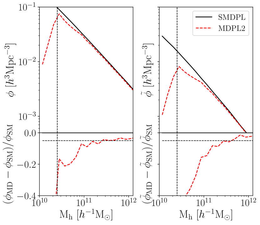
Figure 1: Left panels: Halo mass function (HMF) of the simulations mdpl2, $\phi_{\rm MD}$ (red dashed line), and smdpl, $\phi_{\rm SM}$ (black solid line), at redshift $z=0$. The lower-left panel shows the fractional difference between mdpl2 and smdpl halo mass functions. Note that for masses lower than $10^{11}~{}h^{-1}\,\mathrm{M_{\odot}}$ there are approximately 20 per cent more haloes in smdpl than in mdpl2. Right panels: Subhalo mass function (SHMF) of mdpl2, $\tilde{\phi}_{\rm MD}$ (red dashed line), and smdpl, $\tilde{\phi}_{\rm SM}$ (black solid line), at redshift $z=0$. For masses lower than $10^{11}~{}h^{-1}\,\mathrm{M_{\odot}}$ there are roughly 30 per cent more subhaloes in smdpl than in mdpl2. In both the HMF and SHMF, the vertical dashed line denotes (sub)halo masses of $10^{10.4}$ $h^{-1}$ $\mathrm{M_{\odot}}$. Note that for masses below this limit, the mdpl2 simulation presents a break which establishes the minimum mass above which we can guarantee that we have completeness in the number of haloes for both simulations. The dashed horizontal line indicates a fractional difference of $0.05$.

The rockstar halo finder considers (sub)haloes formed by at least ten dark matter particles, although their properties are not robust when approaching this minimum. According to Behroozi et al. (2013a), halo detection is reliable for structures composed of at least twenty DM particles. Since completeness is important when comparing the 2PCF of different simulations, in this paper we will consider only (sub)haloes with masses greater than $10^{10.4}~{}h^{-1}\,\mathrm{M_{\odot}}$ for both simulations (see vertical dashed lines in Figure 1).

3.2 The two-point correlation function

Given a set of points, the probability of finding an object in an infinitesimal volume $dV$ is $dP=ndV$, where $n$ is the mean number density and $N=nV$ is the number of objects in a finite volume $V$. Then, the 2PCF is defined as the excess probability of finding one of them inside a small volume $dV_{1}$ and the other in a small volume $dV_{2}$, separated by a distance $r$ (Peebles, 1980; Martínez & Saar, 2001), that is

$$dP=n^{2}(1+\xi(r))dV_{1}dV_{2}\,.$$ (8)

In practice, for a catalogue of $N$ particles and volume $V$ with periodic boundary conditions, the 2PCF can be estimated by counting the number of pairs of objects $N_{\mathrm{s}}(r)$, in a shell of volume $V_{\mathrm{s}}(r)$, at distance $r$ from each other using

$$\xi(r)=\frac{1}{n^{2}V}\frac{N_{\mathrm{s}}(r)}{V_{\mathrm{s}}(r)}-1.$$ (9)

However, if the boundaries are not periodic, this equation cannot be applied. This is the case for a real survey, or when we restrict the analysis to a small region within a large periodic simulation. In these cases, the common method consists in comparing the observed data (D) with catalogues composed of random points (R) that reproduce the same geometry and artefacts of the original catalogue. In general, random catalogues contain at least 10 times more objects than the data catalogue, in order to reduce the noise level. In such cases, the 2PCF can be computed using the Landy-Szalay estimator (Landy & Szalay, 1993)

$$\xi(r)=\frac{DD(r)-2DR(r)+RR(r)}{RR(r)}\,.$$ (10)

Here $DD(r)$, $DR(r)$ and $RR(r)$ are the normalized data-data, data-random and random-random pairs, respectively. If $N_{\mathrm{d}}$ and $N_{\mathrm{r}}$ are the number of objects in D and R then

$$DD(r)=\frac{dd(r)}{N_{\mathrm{d}}(N_{\mathrm{d}}-1)/2}\,,$$ (11)

$$RR(r)=\frac{rr(r)}{N_{\mathrm{r}}(N_{\mathrm{r}}-1)/2}\,,$$ (12)

$$DR(r)=\frac{dr(r)}{N_{\mathrm{d}}N_{\mathrm{r}}}\,,$$ (13)

where $dd(r)$ is the number of objects pairs separated by a distance $r$ in D, $rr(r)$ is the number of pairs separated by a distance $r$ in R and $DR(r)$ is the cross-correlation statistic, the number of pairs separated by a distance $r$ with one point taken from D and the other from R (for more details see e.g. Vargas-Magaña et al. 2013). Throughout this work, we use the publicly available python package corrfunc (Sinha & Garrison, 2020) to compute correlation functions.

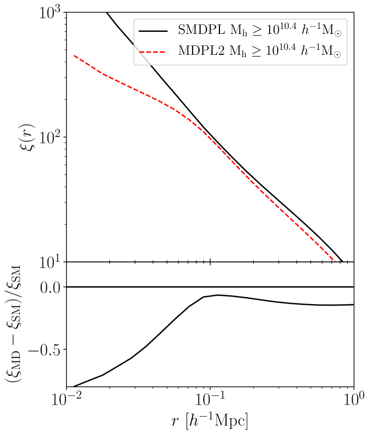
Figure 2: Upper panel: Two-point correlation function (2PCF) for the smdpl (black solid line) and the mdpl2 (red dashed line) simulations at redshift $z=0$. Lower panel: The fractional difference between mdpl2 and smdpl two-point correlation functions. For separations greater than $0.1~{}h^{-1}\,\mathrm{Mpc}$, both simulations present a similar clustering. However, for smaller scales, the clustering functions differ considerably (fractional difference is greater than $0.5$ for scales close to $0.01$). The lower subhalo number fraction in mdpl2, compared with that in smdpl, implies a lower number of pairs at low scales (where the 1-halo term dominates) and, therefore, a lower clustering at those scales.

Figure 2 shows the 2PCF for (sub)halo masses greater than $10^{10.4}~{}h^{-1}\,\mathrm{M_{\odot}}$ for the smdpl (solid line) and mdpl2 (dashed line) simulations at redshift $z=0$. From this figure, we see that the clustering of smdpl is greater than that of mdpl2 for all scales; this effect is more significant at lower scales (between $0.01-0.1~{}h^{-1}\,\mathrm{Mpc}$). The suppression observed in the amplitude of the correlation function of mdpl2 could be due to the use of softened gravity or a finite mass resolution effect. Jenkins et al. (1998) shows that the softening length $\varepsilon$ introduces considerable suppression in the clustering signal only for separations lower than $2\varepsilon$. In our case, mdpl2 is characterised by $\varepsilon=0.005~{}h^{-1}\,\mathrm{Mpc}$, then for scales greater than $0.01~{}h^{-1}\,\mathrm{Mpc}$ the effect of the softening length should be very small. Therefore, the softening length cannot account for the large clustering suppression seen in the mdpl2 simulation for separations between $10^{-2}-10^{-1}~{}h^{-1}\,\mathrm{Mpc}$.

According to the halo model, the 2PCF can be decomposed into two contributions: a 1-halo term and a 2-halo term. The 1-halo term involves correlations between haloes belonging to the same system, i.e. correlations between main host haloes and their corresponding subhaloes and correlations between all subhaloes that belong to a system. On the other hand, the 2-halo term involves correlations between haloes belonging to different systems (Cooray & Sheth, 2002). When the contributions from these two terms are added together, the resulting correlation function should roughly follow a power law (see e.g. Coil 2013). In general, the 2-halo term dominates at large scales (greater than $1~{}h^{-1}\,\mathrm{Mpc}$), while the 1-halo term dominates at scales lower than $1~{}h^{-1}\,\mathrm{Mpc}$. Note that the characteristic scale $\sim 1~{}h^{-1}\,\mathrm{Mpc}$, which is of the order of the size of the main systems, indicates the transition between the two regimes. In van den Bosch et al. (2013), it is shown that increasing the number of subhaloes increases mainly the 1-halo term, because subhaloes are located within host systems of typical sizes $\lesssim 1~{}h^{-1}\,\mathrm{Mpc}$. Therefore, the addition of USHs will enhance the clustering at small scales (Kitzbichler & White, 2008).

For masses between $10^{10.4}-10^{12}~{}h^{-1}\,\mathrm{M_{\odot}}$, the number fraction of subhaloes with respect to total (subhaloes plus main host haloes) is $0.150$ for the smdpl simulation, and $0.124$ for mdpl2. This indicates that, for this mass range, we have roughly 20 per cent more subhaloes in smdpl than in mdpl2. Therefore, we conclude that the discrepancy observed between the 2PCFs of these simulations at small scales (see Figure 2) is a result of the greater number fraction of subhaloes in smdpl compared with mdpl2.

To compensate for this lack of low-mass subhaloes that affects both the SHMF and 2PCF of the low-resolution mdpl2 simulation, we follow the dynamics of the USHs in mdpl2 in a semi-analytic way, by integrating their orbits until they merge with their host halo or are disrupted (see Section 2). We assume that this procedure will provide better agreement with the SHMF and 2PCF provided by the high-resolution smdpl simulation, which we consider adequate functions to constrain the free parameters of our orbital evolution model.

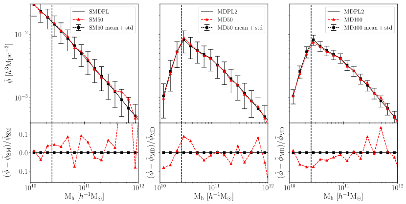
Figure 3: SHMF for the selected calibration and convergence-test boxes compared with those of the full simulations and the mean values obtained from all the subvolumes. Results are shown for the smdpl $50~{}h^{-1}\,\mathrm{Mpc}$ (SM50; left), mdpl2 $50~{}h^{-1}\,\mathrm{Mpc}$ (MD50; centre) and mdpl2 $100~{}h^{-1}\,\mathrm{Mpc}$ (MD100; right). Upper panels: The continuous black line represents the SHMF of the full box of the simulations. The square-dashed black line shows the mean value of the SHMF computed from the small boxes. The error bars correspond to the standard deviation at each subhalo mass bin. Red triangle-dashed lines correspond to the best boxes found to carry out the calibration and convergence-test procedures. Lower panels: Fractional differences in SHMF taking the full simulations as a reference. The vertical line denotes the mass cut at $10^{10.4}~{}h^{-1}\,\mathrm{M_{\odot}}$.

3.3 Calibration and convergence-test volumes

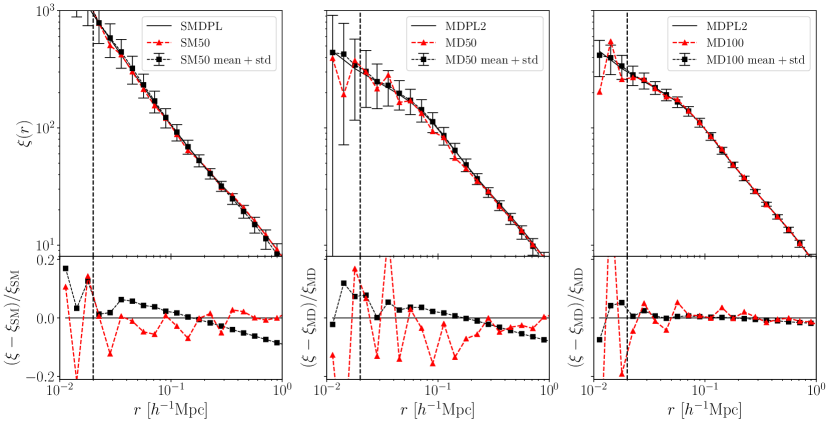
Figure 4: 2PCF for the selected calibration and convergence-test boxes compared to the full simulations and the mean values obtained from all the subvolumes. Results are shown for the smdpl $50~{}h^{-1}\,\mathrm{Mpc}$ (SM50; left), mdpl2 $50~{}h^{-1}\,\mathrm{Mpc}$ (MD50; centre) and mdpl2 $100~{}h^{-1}\,\mathrm{Mpc}$ (MD100; right). Upper panels: The solid black line represents the full simulation. The squared-dashed black line shows the mean value for the 2PCF computed from the small boxes. The error bars correspond to the standard deviation. The red triangle-dashed lines correspond to the best boxes found to carry out the calibration and convergence-test procedures. Lower panels: Fractional differences in 2PCF taking the full simulations as a reference. The vertical dashed line indicates the scale $0.2~{}h^{-1}\,\mathrm{Mpc}$. This limit corresponds to the smaller scale we use to make the comparison since, below this limit, boxes have very few pairs and the correlation function becomes too noisy.

The goal is to make a fast exploration of the parameters of the orbital evolution model, to find regions of the parameter space where there is convergence between the statistical properties obtained from simulations with different mass resolution (i.e., similar SHMF and 2PCF) after applying the orbital evolution model to the simulation with lower resolution. This calibration procedure and the subsequent convergence test that we perform require running the model over both the low-resolution mdpl2 and the high-resolution smdpl simulations. Since this task is computationally very expensive, we are interested in finding a set of boxes that are relatively small in volume but representative of the characteristics of the full simulations. Then, we consider subvolumes of mdpl2 with a box side length of $50~{}h^{-1}\,\mathrm{Mpc}$ and $100~{}h^{-1}\,\mathrm{Mpc}$, and subvolumes of smpdl of $50~{}h^{-1}\,\mathrm{Mpc}$ on a side. Thus, we have the subvolumes mdpl2 $50~{}h^{-1}\,\mathrm{Mpc}$, mdpl2 $100~{}h^{-1}\,\mathrm{Mpc}$ and smdpl $50~{}h^{-1}\,\mathrm{Mpc}$, to which for simplicity we also refer to as MD50, MD100 and SM50, respectively. From the former set of mdpl2 $50~{}h^{-1}\,\mathrm{Mpc}$ subvolumes we extract the best calibration box, while from the latter two sets we obtain the best convergence-test boxes. The choice of these best boxes requires the estimation of their “goodness” (capability of reproducing the characteristics of the full simulations). Here, we exemplify how to obtain the best calibration box, the other cases are analogous.

We partition the full box of mdpl2 into 8000 ($20^{3}$) disjoint subsamples with a box size of $50~{}h^{-1}\,\mathrm{Mpc}$. For each of these boxes, we calculate both $\tilde{\phi}$ and $\xi$. In the case of the 2PCF, $\xi$, we consider only (sub)haloes with masses greater than $10^{10.4}~{}h^{-1}\,\mathrm{M_{\odot}}$, i.e. where the mdpl2 simulation is complete. Using these results, we compute the mean values of the SHMF and the 2PCF, $\langle\tilde{\phi}\rangle$ and $\langle\xi\rangle$, respectively. Analogously, we obtain the mean values $\langle\tilde{\phi}\rangle$ and $\langle\xi\rangle$ for both mdpl2 $100~{}h^{-1}\,\mathrm{Mpc}$ (with $10^{3}$ subvolumes) and smdpl $50~{}h^{-1}\,\mathrm{Mpc}$ (with $8^{3}$ subvolumes).

Figures 3 and 4 show (in square-dashed line) the mean values for the SHMF and 2PCF, respectively. We also plot (in continuous line) the SHMF and 2PCF corresponding to the full simulations. For both figures, we have the following cases: smdpl $50~{}h^{-1}\,\mathrm{Mpc}$ (SM50 mean; left), mdpl2 $50~{}h^{-1}\,\mathrm{Mpc}$ (MD50 mean; centre) and mdpl2 $100~{}h^{-1}\,\mathrm{Mpc}$ (MD100 mean; right). Error bars indicate the standard deviation of the subvolume sets. In Figure 3, we note that, as it happens in the mdpl2 full simulation, the boxes also present a lack of low mass haloes (centre and right). The vertical dashed line indicates the minimum mass we consider in our study ($10^{10.4}$ $h^{-1}$ $\mathrm{M_{\odot}}$). Figure 4 shows the clustering signal. We note that for very low separations ($\lesssim 0.02~{}h^{-1}\,\mathrm{Mpc}$), the scatter in $\xi$ is high, which is reflected in the magnitude of the error bars. This effect is mainly due to the fact that, at these scales, the number of pairs is scarce and therefore Poissonian error dominates.

In order to find the best mdpl2 $50~{}h^{-1}\,\mathrm{Mpc}$ box (hereafter MD50), we need to characterise how representative each of our subsamples is. To estimate how much each box deviates from the full mdpl2 simulation (regarding to the SHMF and 2PCF), and pre-select some boxes that can be good candidates, we compute MAPE (mean absolute percentage error) estimates, i.e., for a given subvolume $j$, we compute the sum over all bins

$$\mathrm{MAPE}\left[h^{(j)}\right]=\frac{1}{n}\sum^{n}_{i=1}\frac{|h^{(j)}_{i}-h_{i}|}{|{h}_{i}|},$$ (14)

where $h$ represents any of the relevant constraining functions (i.e., the $\tilde{\phi}$ or $\xi$), $j$ indicates the given subvolume, and $n$ is the number of bins (mass-bins for $\tilde{\phi}$, separation-bins for $\xi$) where the function is computed. In this expression, ${h}_{i}$ indicates the value of function $h$ in a given bin $i$ corresponding to the full simulation.

As mentioned above, the full mdpl2 simulation is not complete for low masses; furthermore, the correlation function computed in subvolumes becomes too noisy for scales below $0.02~{}h^{-1}\,\mathrm{Mpc}$. Taking this into account, for each subvolume we only consider $\mathrm{MAPE}\left[\tilde{\phi}\right]$ errors for masses higher than $10^{10.4}~{}h^{-1}\,M_{\odot}$ and $\mathrm{MAPE}\left[\xi\right]$ errors for separations in the range $0.02-1~{}h^{-1}\,\mathrm{Mpc}$. We choose candidates for the best MD50 box as the ones that simultaneously minimize both $\mathrm{MAPE}\left[\tilde{\phi}\right]$ and $\mathrm{MAPE}\left[\xi\right]$. From these candidates, we choose our final best calibration box by visual inspection.

The method applied to find the best convergence-test subvolumes smdpl $50~{}h^{-1}\,\mathrm{Mpc}$ (hereafter SM50) and mdpl2 $100~{}h^{-1}\,\mathrm{Mpc}$ (hereafter MD100) is analogous to what we have done for the calibration box MD50. Figure 3 shows in triangle-dashed red line the SHMF of the best subvolumes SM50 (left), MD50 (center) and MD100 (right); the SHMF of SM50 is slightly higher than the mean for masses close to $10^{12}~{}h^{-1}\,\mathrm{M_{\odot}}$. Likewise, Figure 4 shows in triangle-dashed red lines the 2PCF of the best subvolumes for the same sets. The vertical dashed lines in Figures 3 and 4 indicate, respectively, the mass cut (for the SHMF; $10^{10.4}~{}h^{-1}\,\mathrm{M_{\odot}}$) and the smallest scale (for the 2PCF; $0.2~{}h^{-1}\,\mathrm{Mpc}$) we use to make the comparison with the corresponding mean values. In the case of the 2PCF, we can see that, below this limit, boxes have very few pairs and the correlation function becomes too noisy. These results show that we are able to find smaller boxes, representative of the complete simulation boxes, to carry out the parameter exploration and the subsequent convergence test.

4 Results

In this section, we make an exploration of the parameter space of the orbital evolution model of USHs applied to the low-resolution mdpl2 simulation by evaluating the changes produced on the SHMF and 2PCF when the free parameters of the model are varied. We recall the meaning of the parameters under consideration: $b$ characterises the dynamical friction through the Coulomb logarithm (equation 4), $\alpha$ controls the TS (equation 6) and $f$ is related to the merger criterion (equation 7).

Figure 5 shows the results obtained after applying the orbital evolution model to the calibration MD50 subvolume introduced in Section 3. Here, we plot fractional differences taking the full smdpl simulation as a reference, and selecting all (sub)haloes with masses greater than $10^{10.4}~{}h^{-1}\,\mathrm{M_{\odot}}$ at redshift $z=0$. The top panels show fractional differences in the SHMF while the bottom panels show fractional differences in the 2PCF. The solid black line indicates the fractional difference between the mdpl2 and smdpl full simulations, while the dotted black line indicates the fractional difference between the MD50 calibration box and the smdpl full simulation. The dashed lines with symbols correspond to fractional differences obtained after applying the orbital evolution model to the MD50 calibration box, considering different parameter combinations of the model. In all panels, the dashed-circle black line corresponds to the same fiducial parameters $(b=0.50,f=0.05,\alpha=2.0)$. From left to right, we vary $b$ (left panels), $f$ (centre panels) and $\alpha$ (right panels), leaving the remaining parameters fixed to their fiducial values. In any case, when applying the orbital evolution model to the USHs, both the SHMF and 2PCF increase with respect to the results obtained from the mdpl2 simulation, as expected. In the following subsections, we analyse the impact on the SHMF and the 2PCF of varying the different free parameters of our model.

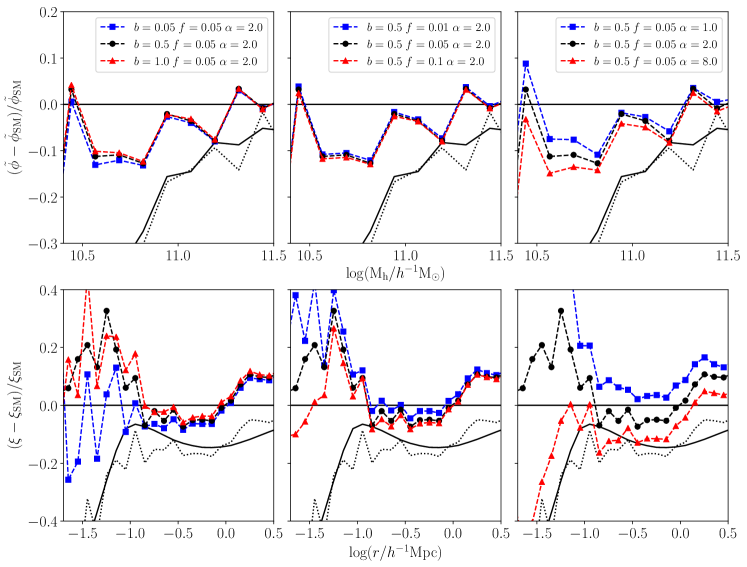
Figure 5: Fractional differences in SHMF (top panels) and in 2PCF (bottom panels) with respect to the smdpl full simulation for a sample obtained from applying the orbital evolution model to USHs of the MD50 calibration box considering different combinations of values of the model parameters (dashed lined with symbols). The dashed-circle black line corresponds to the same fiducial parameters $(b=0.50,f=0.05,\alpha=2.0)$ in all panels. Solid and dotted lines correspond to the fractional difference with respect to smdpl for the mdpl2 simulation and the MD50 calibration box, respectively. Left panels: Effect of varying the parameter $b$ leaving $f$ and $\alpha$ fixed. Parameter $b$ enters the dynamical friction force term through the Coulomb logarithm, $\ln({\Lambda})$. Decreasing this parameter increases $\ln({\Lambda})$ and the DF effect, thus more USHs merge with their hosts and $\tilde{\phi}$ decreases. Since we have a smaller number fraction of USHs, the clustering signal $\xi$ also decreases. Central panels: Different values of the parameter $f$ leaving $b$ and $\alpha$ fixed. The value of $f$ determines the minimum distance an USH can be from the centre of its host before it is considered merged with it. Increasing this parameter implies a higher number of mergers and a lower number of USHs. This also impacts on the clustering signal $\xi$, which decreases. Right panels: Effect of varying $\alpha$ leaving $b$ and $f$ fixed. Increasing the value of $\alpha$ implies greater efficiency of the TS process and, consequently, greater mass loss which leads to a lower number of USHs with mass above the threshold $10^{10.4}~{}h^{-1}\,\mathrm{M_{\odot}}$ considered to estimate the SHMF and the 2PCF. As we have fewer USHs, then both $\tilde{\phi}$ and $\xi$ decrease.

4.1 Variation of parameter $b$

The parameter $b$ enters the DF force term through the Coulomb logarithm (see equations 1 and 4). Decreasing $b$ is equivalent to increasing the value of the Coulomb logarithm $\ln(\Lambda)$ and this leads to a greater deceleration of USHs due to DF drag and, consequently, a greater number of USHs that reach the central part of their host haloes. At first order, DF effect would only introduce changes in the spatial distribution of USHs, but mergers and TS may work in favour of modifying the number of USHs of a given mass. The impact of the changes in the parameter $b$ on the SHMF, $\tilde{\phi}$, is shown in the upper-left panel of Figure 5 (dashed lines with symbols). Increasing (decreasing) $b$ results in a higher (lower) number of total USHs, and $\tilde{\phi}$ increases (decreases). These changes are more noticeable for low-mass USHs. Although DF works more efficiently for more massive USHs, driving them to the inner parts of the host halo, the number of USHs that merge with their hosts is not high enough to produce a significant decrease in the SHMF. Indeed, for $b=0.05$, the lowest value of the parameter $b$ considered in this analysis, the number fractions of merged USHs (regardless of their mass) are $\sim 0.05$, $0.04$ and $0.01$ at $z=2,1,0$, respectively. On the other hand, those USHs that do not merge are subjected to TS. This process becomes more efficient as the USHs move closer to the host centre (effect more pronounced for lower values of $b$). Therefore, when the mass of an USH is reduced by TS, it may be either disrupted or may fall below the mass cut considered in our analysis ($10^{10.4}~{}h^{-1}\,\mathrm{M_{\odot}}$), leading to a change in the SHMF at low masses (see further discussion in Section 4.3).

The lower-left panel of Figure 5 shows the impact of the changes in the parameter $b$ on the 2PCF, $\xi$ (dashed lines with symbols). The clustering signal increases (decreases) with the increase (decrease) of $b$ as a result of the increase (decrease) of the number fraction of USHs. The changes in $\xi$ are larger at small scales. Since decreasing $b$ implies that USHs decay faster towards the central part of their host halo, one might expect there should be an increase in clustering at lower scales. However, this does not occur because many of these USHs end up either merging with their main host halo or disrupting, and therefore do not contribute to the 2PCF.

4.2 Variation of parameter $f$

The parameter $f$ is related to the merger criterion. Increasing (decreasing) the value of $f$ increases (decreases) the distance range within which USHs are considered to merge with their hosts. Therefore, a higher value of $f$ implies shorter merging time-scales, a greater number of mergers and a lower number of total USHs. These trends affect both the SHMF and the 2PCF, as can be seen, respectively, in the upper-central and lower-central panels of Figure 5, which show the results of the orbital evolution model for different values of the parameter $f$. Thus, for a value of $f$ higher than the fiducial value, both the SHMF and the 2PCF decrease because of the lower number of USHs, while for a lower value of $f$ both the SHMF and the 2PCF increase. However, the impact on the SHMF is minimal; the number of mergers is not significantly affected by the changes in $f$, and USHs of any mass are involved in the merging process. For any value of $f$, the value of the correlation function $\xi$ is larger for separations below $\log(r/h^{-1}\mathrm{Mpc})\leq-1$ than at intermediate separations, i.e. $\log(r/h^{-1}\mathrm{Mpc})\geq-1$. Note that the increase in clustering signal obtained at low scales is more pronounced for a lower value of $f$ because the 1-halo term of $\xi$ depends strongly on the number fraction of subhaloes, which is higher in this case.

4.3 Variation of parameter $\alpha$

The parameter $\alpha$ controls the rate at which the TS mechanism removes mass from an USH. The top-right and bottom-right panels of Figure 5 show, respectively (in dashed lines with symbols), the SHMF and the 2PCF for different values of $\alpha$. As the value of $\alpha$ increases, TS becomes more efficient and more material is removed from an USH via this process, leading to a reduction in the values achieved by the SHMF and the 2PCF. These trends are a result of the competition of two aspects. On one hand, the change of mass of the USHs as a result of TS have direct impact on their merging time-scales, i.e. a lower mass implies a lower dynamical friction force (equation 1), leading to a larger number of USHs of lower mass that have not merged. On the other hand, some of the USHs subjected to mass removal might become disrupted leading to a decrease in the number fraction of USHs. Moreover, the mass of those USHs that have been neither disrupted nor merged may fall below the mass cut considered to estimate the SHMF and the 2PCF producing, respectively, a general decrease at all masses and scales. Indeed, after applying the orbital evolution model with the best-fitting parameters (see the following section), $\sim 90$ per cent of the USHs have masses below $10^{10.4}~{}h^{-1}\,\mathrm{M_{\odot}}$ at $z=0$.

4.4 Best-fitting parameters

To find the best-fitting value of each free parameter, we perform an exploration of the parameter space running the orbital evolution model over the calibration box MD50 and varying the values of the parameters $b$, $f$ and $\alpha$. For parameter $b$, we consider values in the range $0.05-1.0$. We allow $f$ to vary between $0.01-0.10$. The parameter $\alpha$ takes values between $1.0-8.0$. For each run output, we compute the corresponding SHMF (for subhaloes with masses greater than $10^{10.4}~{}h^{-1}\,\mathrm{M_{\odot}}$) and the 2PCF (for haloes and subhaloes of masses greater than $10^{10.4}~{}h^{-1}\,\mathrm{M_{\odot}}$) at redshift $z=0$. We then compare the values of these functions with those of smdpl using a cost function given by

$$C(b,f,\alpha)= \frac{1}{N_{1}}\sum_{j=1}^{N_{1}}\ln^{2}\left(\frac{\tilde{\phi}^{j}_{\mathrm{model}}(b,f,\alpha)}{\tilde{\phi}^{j}_{\mathrm{\sc SM}}}\right)+$$ (15)

$$\frac{1}{N_{2}}\sum_{j=1}^{N_{2}}\ln^{2}\left(\frac{{\xi}^{j}_{\mathrm{model}}(b,f,\alpha)}{{\xi}^{j}_{\mathrm{\sc SM}}}\right),$$

where $\tilde{\phi}^{j}_{\mathrm{\sc SM}}$ and ${\xi}^{j}_{\mathrm{\sc SM}}$ correspond to the SHMF and 2PCF of the smdpl simulation, $\tilde{\phi}^{j}_{\mathrm{model}}$ and ${\xi}^{j}_{\mathrm{model}}$ are the corresponding SHMF and 2PCF that result from applying the orbital evolution model to the MD50 calibration box for a particular combination of the parameters $b,f$ and $\alpha$, and $N_{1}$ and $N_{2}$ are the number of mass-bins and separation-bins used to estimate the calibration functions $\tilde{\phi}^{j}_{\mathrm{\sc SM}}$ and ${\xi}^{j}_{\mathrm{\sc SM}}$, respectively. Then, we select the best-fiting values of these parameters as those that minimize the cost function (equation 15). The most suitable parameters found with this method are $b=0.3$, $f=0.036$, and $\alpha=3.0$.

4.5 Convergence test

We conduct a convergence test by comparing results obtained for the calibration box MD50 with those for the convergence-test boxes, MD100 and SM50, introduced in Section 3.3. Such comparison involves results obtained by considering only resolved subhaloes, on one hand, and by adding the USHs, on the other. Comparisons between MD50 and MD100 with and without USHs are done to evaluate the impact of the box size on the results obtained. Comparisons of results for MD50 with and without USHs with those obtained for the full smdpl simulation and the SM50 subvolume have the purpose of validating the orbital evolution model and its best-fitting parameters. Thus, we run the orbital evolution model using the best-fitting parameters over the boxes MD50, MD100 and SM50. The results of this exercise are shown (in dashed lines with symbols) in Figure 6 and Figure 7 for the SHMF and 2PCF, respectively. The results for the boxes without the inclusion of USHs are depicted as dotted lines with symbols. As a reference, we plot the mdpl2 full simulation (in dashed line) and the smdpl full simulation (in continuous line). In the lower panel of these figures, we show fractional differences taking the smdpl full simulation as a reference.

From Figure 6 we can see that, after applying the orbital evolution model to follow USHs, a good agreement with the smdpl full simulation is achieved for the different boxes (dashed lines with symbols), compared with the behaviour obtained considering only the detected subhalos in those boxes (dotted lines with symbols). We also notice that both MD50 and SM50 present some “spikes” at masses of the order of $10^{12}~{}h^{-1}\,\mathrm{M_{\odot}}$; this is a particular characteristic of the selected boxes. The inclusion of USHs in SM50 (dashed line with squares) has little impact on the SHMF. This is quantified by estimating the number density of subhaloes for the mass range above the mass cut considered ($10^{10.4}~{}h^{-1}\,\mathrm{M_{\odot}}$): $\sim 0.0172~{}h^{3}\,\mathrm{Mpc}^{-3}$ for SM50, and $\sim 0.0201~{}h^{3}\,\mathrm{Mpc}^{-3}$ for SM50 with USHs (SM50$+$model). For MD50, we note that the addition of USHs (dashed line with circles) helps to enhance the SHMF at low masses; the number density of all resolved subhaloes in MD50 is $\sim 0.0121~{}h^{3}\,\mathrm{Mpc}^{-3}$, and the number density obtained after adding USHs increases to $\sim 0.0177~{}h^{3}\,\mathrm{Mpc}^{-3}$, achieving a very good agreement with the value obtained for SM50. Note that these number densities depend on the chosen subvolumes. Differences between MD50 and SM50 also arise because mdpl2 not only presents a deficiency in subhaloes but also of main host systems compared with smdpl. The SHMF obtained for MD50 after adding UHSs (MD50$+$model) converges to the SHMF of the full smdpl; the mean fractional difference over the entire mass range is $\sim 10$ per cent. Finally, the results obtained for both MD100 (dotted line with triangles) and MD100$+$model (dashed line with triangles) are very similar to those obtained for MD50 and MD50$+$model, respectively, indicating that the size chosen for the calibration box is adequate to carry out the calibration procedure.

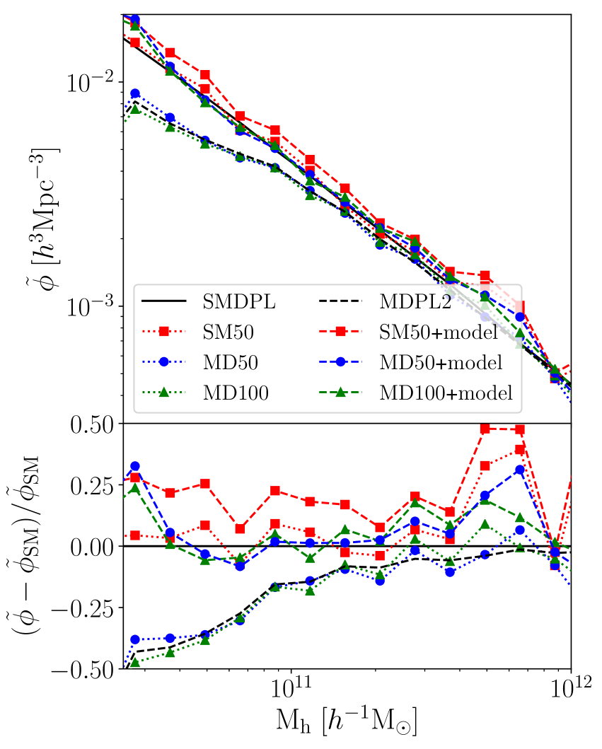
Figure 6: Upper panel: Subhalo mass functions. Dotted lines with symbols correspond to calibration and convergence-test boxes (see Section 3.3) without the inclusion of USHs. Dashed lines with symbols correspond to the those boxes after applying the orbital evolution model using the best-fitting parameters (see Section 4.4). We consider the mdpl2 calibration box MD50, and the convergence-test boxes MD100 and SM50. The simple dashed line denotes the mdpl2 full simulation and the continuous line corresponds to the smdpl full simulation. Lower panel: Fractional differences taking the smdpl full simulation as a reference. We see that after applying the model to track the orbital evolution of USHs in SM50 and MD50, the difference is $\sim 10$ per cent for the entire mass range.

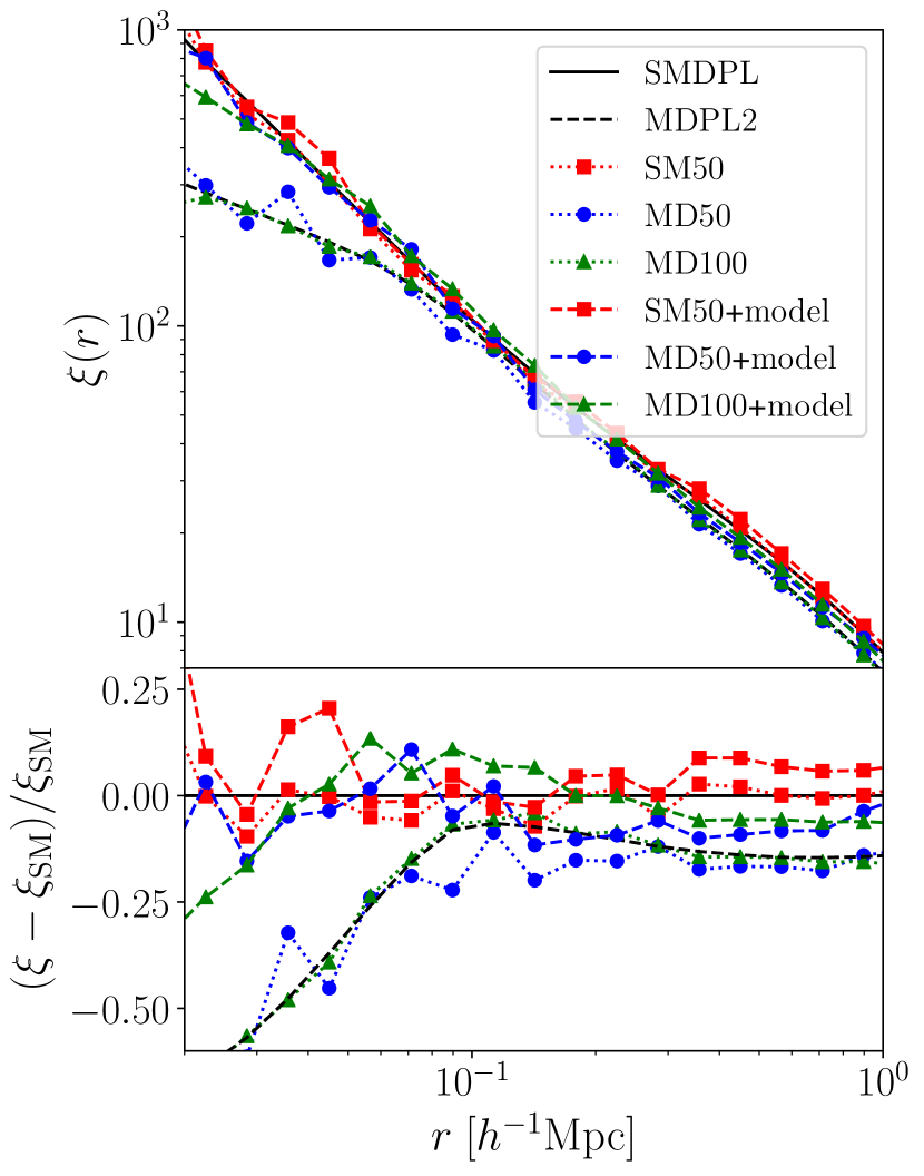
Figure 7: Two-point correlation functions. Dotted lines with symbols correspond to the calibration and convergence-test boxes without the inclusion of USHs. Dashed lines with symbols correspond to the samples obtained for these boxes after applying the orbital evolution model using the best-fitting parameters. We consider the calibration box MD050, and the convergence-test boxes MD100 and SM050. The simple dashed line denotes the full mdpl2 simulation and the continuous line corresponds to the full smdpl simulation. Lower panel: Fractional differences in the 2PCFs taking the full smdpl simulation as a reference. After applying the model, we obtain an enhancement of the clustering for both MD050 and MD100. In general, the agreement between the different boxes is within 10 per cent except for scales below $0.03~{}h^{-1}\,{\rm Mpc}$, where the agreement is within 20 per cent.

Figure 7 shows the effect on the 2PCF of running the orbital evolution model over the calibration and convergence-test boxes using the best-fitting parameters. In general, tracking the orbital evolution of USHs in MD50 and MD100 (MD50$+$model and MD100$+$model, respectively) considerably improves the 2PCF, increasing the signal over the entire range of scales (dashed lines with symbols) compared to the results obtained considering only the detected substructures in those boxes (dotted lines with symbols). Note that for both mdpl2 subvolumes in the latter case, the clustering is strongly suppressed with respect to the one obtained for the full smdpl simulation with a discrepancy greater than 50 per cent for scales close to $0.02~{}h^{-1}\mathrm{Mpc}$. The enhancement obtained when including USHs is more pronounced at small scales ($0.02-0.10~{}h^{-1}\,\mathrm{Mpc}$) where the 1-halo term dominates, which mainly depends on the number fraction of satellite haloes. In general, mean fractional errors for the 2PCF over the whole range of scales considered are within 10 per cent for all calibration and convergence-test boxes (i.e. MD50, MD100 and SM50) when adding USHs. From these results, we can conclude that the inclusion of USHs improves the SHMF and 2PCF of the simulation with lower resolution (mdpl2) leading to a better agreement with the results obtained for the higher-resolution one (smdpl).

With this analysis, we have shown that, on the one hand, the smdpl simulation has an almost complete population of subhaloes above $10^{10.4}~{}h^{-1}\,\mathrm{M_{\odot}}$. Indeed, if we apply the orbital evolution model to a smaller fraction of smdpl, namely SM50, we obtain almost the same SHMF and 2PCF as in the full simulation. The differences between smdpl and its SM50 box after the application of the model are a result of the presence of unresolved systems in smdpl, and are only noticeable at the smallest masses (in the SHMF) and smallest scales (in the 2PCF); these differences are small and we can safely neglect them. This fact supports the use of the smdpl simulation as a reference for the exploration of the parameters of the orbital evolution model. On the other hand, the results obtained for the MD50 and MD100 boxes after including USHs are consistent (the observed differences are a result of the selected box). Clearly, the size of the MD50 box is sufficiently good to tune the free parameters of the model, and it is not necessary a larger box for this purpose.

5 Validation of the calibration procedure

Recently, van den Bosch & Ogiya (2018) investigated the circumstances in which subhaloes identified in cosmological simulations undergo disruption, arriving at the conclusion that most disruptions are numerical in origin. Using a large suite of idealized simulations in which subhaloes move in a fix, external potential, they analyse under what conditions inadequate force softening and discreteness noise have an impact on subhaloes. In their work, the authors present two criteria (applied to the bound mass fraction $f_{\rm bound}$ of subhaloes) to assess whether individual subhaloes in cosmological simulations are reliable or not. In our work, we estimate $f_{\rm bound}$ as the ratio between the mass of the subhalo at a given time and its mass at accretion. They claim that the subhaloes that satisfy either of these two criteria should be discarded from further analysis. Specifically, they find that subhaloes start to be significantly affected by discreteness noise when

$$f_{\rm bound}<0.32\left(\frac{N_{\rm acc}}{1000}\right)^{-0.8},$$ (16)

where $N_{\rm acc}$ is the number of particles in the subhalo at accretion. Furthermore, subhalos are systematically affected by inadequate force resolution when

$$f_{\rm bound}<\frac{1.79}{f(c)}\left(\frac{\varepsilon}{r_{\mathrm{s},0}}\right)\left(\frac{r_{\rm h}}{r_{\mathrm{s},0}}\right),$$ (17)

where $r_{\mathrm{s},0}$ and $c$ are the scale radius and concentration parameter of the (NFW) subhalo at accretion, respectively, $f(x)=\ln{(1+x)}-x/(1+x)$, $\varepsilon$ is the characteristic softening length of the simulation and $r_{\mathrm{h}}$ is the instantaneous half-mass radius. Both situations could lead to artificial disruptions and, therefore, they are considered as criteria to discard subhaloes.

The authors indicate that DM subhaloes are artificially disrupted even in state-of-the-art cosmological N-body simulations. Therefore, one could argue that the smdpl simulation, which is taken as reference in the present work, may be subjected to numerical artifacts that affect the tidal evolution of the DM subhaloes. If we apply those criteria to the cosmological simulations that we are using in our analysis, most of the subhaloes would not survive. In fact, this would be true for many of the available simulations in the literature, since those findings are applicable to all the subhaloes identified in any cosmological simulations. However, the results of any study that analyse the convergence between simulations computed with similar techniques will still be valid and useful for modelling structure formation.

In our case, we are studying the convergence between two simulations (mdpl2 and smdpl) with different mass and spatial resolutions that have been selected from the same family (MultiDark-Planck simulations), i.e., they have been generated using the same methodology and cosmology, and have been analysed with the same halo finder (rockstar). Therefore, they suffer similar numerical artifacts. The method that we use to select the parameters that best fit our orbital evolution model, which is applied to the USHs of the lower-resolution simulation (mdpl2), tries to find the convergence of some global statistical properties (i.e. SHMF and 2PCF) between both simulations.

To assess the robustness of the calibration procedure used to determine the best-fitting parameters of the orbital evolution model presented in this work, we perform a comparison between the orbits followed by a set of resolved subhaloes in the SM50 box (smdpl $50~{}h^{-1}\,\mathrm{Mpc}$, see section 3.3), that are reliable according to the criteria presented in van den Bosch & Ogiya (2018) (i.e. they do not satisfy neither equation (16) nor equation (17)), and the orbits of those same resolved subhaloes predicted by our orbital evolution model. Such comparison is quantified by analysing the distribution of values adopted by the free parameters of the model. The aim is to evaluate if they are consistent with the values of the best-fitting parameters found using the SHMF and 2PCF as constraints (section 4.4).

In this analysis, we consider the circularity of bound orbits (negative total energy, $E<0$). The circularity is defined as the ratio of the orbital angular momentum, $L$, to the angular momentum of a circular orbit with the same energy, $L_{\mathrm{\mathrm{circ}}}(E)$. Hence, the circularity of an orbit is given by

$$\eta=\frac{L}{L_{\mathrm{\mathrm{circ}}}(E)}=\frac{L}{r_{\mathrm{circ}}\,\mu\,V_{\mathrm{circ}}},$$ (18)

where $r_{\mathrm{circ}}=-GM_{\mathrm{host}}M_{\mathrm{sub}}/E$, $V_{\mathrm{circ}}=\sqrt{-2E/\mu}$, and $\mu=M_{\mathrm{host}}M_{\mathrm{sub}}/(M_{\mathrm{host}}+M_{\mathrm{sub}})$ is the reduced mass of the host-subhalo system (Khochfar & Burkert, 2006).

To carry out the comparison, we select reliable subhaloes (according to van den Bosch & Ogiya (2018) criteria) that survive in the SM50 box for a minimum of $25$ snapshots. For each subhalo, we compute the circularity along its orbit according to equation 18. We further separate the subhaloes in bins of circularity, keeping only those with stable circularity (i.e. those for which its circularity at different snapshots does not deviate more than 0.15 from its mean circularity estimated during the period of time in which we compare the actual orbit with the one simulated by our model). We run the orbital evolution model for these subhaloes and estimate separately the values of the parameter $b$, involved in the DF model (Section 4.1), and the parameter $\alpha$, associated to TS (section 4.3). We do not estimate the parameter involved in the proximity merger criterion, $f$ (section 4.2), because several subhaloes in the sample selected for this analysis remain resolved up to $z=0$, that is, they do not merge with their host. We then proceed in the following way:

1. Firstly, we estimate the value of the parameter $b$ by running the orbital evolution model with different values of this parameter. Although DF affects both the positions and velocities of the subhaloes, we focus on the former. In order to avoid the impact of the TS modelling, the mass and radius of the subhalo ($M_{\rm ush}$ and $R_{\rm ush}$ in equations 1 and 4, respectively) are assigned according to the values that those quantities take along the orbit in the smdpl cosmological simulation. Then, we compare the evolution of the positions of the subhaloes in our sample (taken from the SM50 box) with that predicted by the orbital evolution model (equations 1 and 4).

2. Secondly, we estimate the value of the parameter $\alpha$ involved in the TS model, which affects the mass of the subhaloes, by varying this parameter in the orbital evolution model. In this case, we do not consider the DF modelling, and the positions and velocities of the subhaloes are extracted from the smdpl cosmological simulation. Then, we compare the evolution of the mass of the subhaloes in our sample (taken from the SM50 box) with the evolution of the mass as predicted by our model (equations 5 and 6).

To quantify the similarity of the actual orbit of the subhaloes with the orbit simulated by our orbital evolution model, we construct a cost function that is the sum of the logarithmic squared differences between these two types of orbits along the time. We use many orbits to perform the analysis, and average the cost functions of all of them as our final cost function $C(p)$. This cost function depends on the parameters $p$ of the orbital evolution model (either $b$ or $\alpha$), and its minimum indicates which is the model parameter for which the likeness is the best. Hence, the cost function is

$$C(p)=\sum_{i=1}^{N_{\mathrm{sim}}}\frac{C_{i}(p)}{N_{\mathrm{sim}}},$$ (19)

where $C_{i}(p)$ is the cost function for each orbit, which depends on the parameter $p$, and $N_{\mathrm{sim}}$ is the number of orbits included in the analysis. In this analysis we consider $N_{\mathrm{sim}}=25$.

For the parameter $b$, the cost function of a single orbit is

$$C_{i}(b)=\frac{1}{N^{i}_{\mathrm{evals}}}\sum_{j=1}^{N^{i}_{\mathrm{evals}}}\ln^{2}\left(\frac{r^{i}_{\mathrm{model}}(t_{j},b)}{r^{i}_{\mathrm{\sc SM50}}(t_{j})}\right).$$ (20)

Here, $r^{i}_{\mathrm{model}}(t_{j},b)$ is the radial distance from the subhalo to the centre of the host obtained from the orbital evolution model, where $b$ is the varied parameter and $t_{j}$ is the point of evaluation (in the orbit); $r^{i}_{\mathrm{\sc SM50}}(t_{j})$ is the value of radial distance along the actual orbit extracted from the SM50 box. Since the selected subhaloes have different lifetimes, the number of evaluations, $N^{i}_{\mathrm{evals}}$, depends on the orbit considered.

For the parameter $\alpha$, the cost function for a single orbit is

$$C_{i}(\alpha)=\frac{1}{N^{i}_{\mathrm{evals}}}\sum_{j=1}^{N^{i}_{\mathrm{evals}}}\ln^{2}\left(\frac{m^{i}_{\mathrm{model}}(t_{j},\alpha)}{m^{i}_{\mathrm{\sc SM50}}(t_{j})}\right).$$ (21)

In this case, we compare the mass of the subhalo provided by the smdpl simulation (SM50 box), $m^{i}_{\mathrm{\sc SM50}}(t_{j})$, with that computed by applying the orbital evolution model, $m^{i}_{\mathrm{model}}(t_{j},\alpha)$, where $\alpha$ is the varied parameter and $t_{j}$ is the point of evaluation (in the orbit).

Figure 8 shows the cost function for different values of $b$, both for subhaloes contained in different circularity bins (dashed lines with symbols) and for the full sample of selected haloes (continuous line). We note that the value of $b$ that minimize the cost function depends on the value of the circularity of the orbits. For the complete sample considered for this analysis, we obtain that a value of $b=0.225$ (black-star symbol) optimise the similarity between the orbits of the resolved subhaloes in the SM50 box and the corresponding orbits predicted by the orbital evolution model.

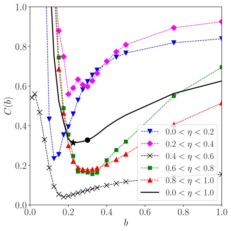
Figure 8: Cost function for the parameter $b$ for subhaloes selected from the SM50 box. Dashed lines with symbols correspond to subhaloes lying within different circularity bins, while the continuous line represents the full sample of subhaloes. The value of $b$ that minimizes the cost function depends on the circularity of the orbit. The black-circle represents the cost function for the best-fitting parameter $b=0.3$. The black-star symbol, located at $b=0.225$, indicates the minimum value of the cost function for the sample of subhaloes analysed here.

Figure 9 shows the cost function for different values of the parameter $\alpha$. In dashed lines with symbols, we show the cost function for subhaloes lying in different circularity bins, while the continuous line corresponds to the cost function of the full sample. The parameter $\alpha$ also depends on the value of the circularity of the orbit, showing a clear trend. This is reasonable, since for more circular orbits (large values of $\eta$), the subhalo will not reach the innermost part of the host gravitational potential and, hence, it will be less affected by TS (lower values of $\alpha$). On the contrary, less circular orbits (more elongated ones) will reach the innermost parts of the host potential, being subjected to a larger tidal stripping effect, resulting in larger values of the parameter $\alpha$. When using the complete sample of selected subhaloes, the cost function is minimized for $\alpha=3.75$ (black-star symbol).

The value of the cost functions for the best fitting parameters $b=0.3$ and $\alpha=3.0$, are represented by black-circles in Figures 8 and 9, respectively. Note that these values are consistent with the values $b$ and $\alpha$ that we get when analysing individual orbits of reliable subhaloes, according to the criteria of van den Bosch & Ogiya (2018), that is, by using the SHMF and the 2PCF to constrain the free parameters of the orbital evolution model. Moreover, our methodology, which involves such global statistics, naturally takes into account, and average out, the different behaviours that we see for different circularities. Hence, the results of this analysis give strong support to the calibration procedure applied to our orbital evolution model.

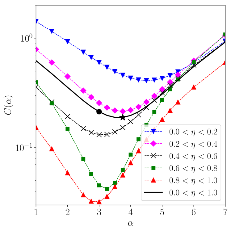
Figure 9: Cost function for the parameter $\alpha$ for subhaloes selected from the SM50 box. Dashed lines with symbols correspond to subhaloes lying within different circularity bins, while the continuous line represents the full sample of subhaloes. The value of $\alpha$ that minimizes the cost function depends on the circularity of the orbit. The black-circle indicates the cost function for the best-fitting parameter $\alpha=3.0$. The black-star symbol, located at $\alpha=3.75$, corresponds to the minimum value of the cost function for the sample of subhaloes analysed here.

6 Discussion

We present a model to track the orbital evolution of USHs and propose a method to calibrate its free parameters. From the analysis presented above we have that, in general, the inclusion of USHs in the statistical analysis of the properties of substructures (e.g. mass and phase-space coordinates) detected in a DM-only simulation is key to achieving a better agreement with the results obtained from a higher-resolution simulation in which the number of USHs is smaller. Here, we discuss in more detail some aspects of our results.

The inclusion of USHs helps to enhance the SHMF over the entire mass range. However, as we can see from the upper-panels of Figure 5, the SHMF depends more strongly on the parameter $\alpha$ (related to TS, which changes the mass of the USH), than on the parameters $b$ (involved in DF) and $f$ (considered in the merger proximity criterion). Indeed, varying $b$ and $f$ has little impact on the overall shape and normalisation of the SHMF. Since $b$ and $f$ are related mainly to the evolution of the position of the USHs, the SHMF fails to put a tight constraint on those parameters.

The main contribution of the calibration procedure proposed in this work is the inclusion of the 2PCF as a constraining function, which is sensitive to variations of the three parameters involved in our orbital evolution model (see lower panels of Figure 5), although the behaviour is different depending on the scales considered. For very small scales ($\lesssim 0.3~{}h^{-1}\,\mathrm{Mpc}$), the correlation function is dominated by the 1-halo term (van den Bosch et al. 2013) which depends strongly on the number fraction of subhaloes. Then, this region is very sensitive to variations of the parameters involved in the dynamical friction model ($b$ and $\alpha$ through the Coloumb Logarithm and the subhalo mass, respectively) or the merging criterion ($f$). At greater separations ($\gtrsim 0.3~{}h^{-1}\,\mathrm{Mpc}$), the 2-halo term begins to compete against the 1-halo term, and the constraining power of the correlation function is reduced. It is worth noting that if the strength of TS is high ($\alpha\sim 8.0$), then the clustering is strongly suppressed at small scales. Hence, while the SHMF fails to constrain $b$ and $f$, the 2PCF has great constraining power on all free parameters of the model. As a result of the exploration of the parameter space considering the SHMF and 2PCF as constraints, we find the following best-fitting parameters: $b=0.3,f=0.036,\alpha=3.0$.

Previous works in the literature explore the possible values that the Coulomb logarithm can take. Pullen et al. (2014) assume a fixed value $\ln(\Lambda)=2$. Other authors choose the value of the Coulomb logarithm in order to reproduce the results of numerical simulations. For example, Velazquez & White (1999), by studying orbits in N-body simulations, find values of $\ln(\Lambda)$ within the range $1-2$. Using a model similar to the one presented here, Yang et al. (2020) find $\ln(\Lambda)\sim 1.5$ from the parameter space exploration. In our case, for the best-fitting parameter $b=0.3$, the range of values covered by the Coulomb logarithm implemented in the orbital evolution model (equation 4) is $0-7$. The minimum value, $\ln(\Lambda)=0$, indicates that the DF term can only produce deceleration, and is adopted when $r_{\rm ush}\leq bR_{\rm ush}$. Clearly, the maximum value of the Coulomb logarithm we obtain is larger than those found in previous works, but it is consistent with a broad estimation based on the typical values of the virial radius of haloes (and subhaloes). In our simulations, these radii are in the range $10-1000~{}h^{-1}\,\mathrm{kpc}$. Then, assuming a maximum satellite-host centre distance $r_{\rm ush}$ of the order of the virial radius of main systems, we have that, at most, $r_{\rm ush}/R_{\rm ush}\sim R_{\rm host}/R_{\rm ush}\sim 100$. This gives an estimated maximum value of the Coulomb logarithm of $\ln(\Lambda)_{\mathrm{max}}\sim 6.2$, consistent with that obtained when applying the orbital evolution model. In the latter case, the mean value of the distribution of Coulomb logarithm at $z=0$ is $\ln(\Lambda)\sim 3.6$.

The discrepancy between the mean value of the Coulomb logarithm we have derived and those reported by Velazquez & White (1999), Pullen et al. (2014) and Yang et al. (2020) could be attributed to several reasons. On one hand, the results of these works were obtained by adopting a constant value for $\ln(\Lambda)$, whereas in our orbital evolution model we assume a Coulomb logarithm that varies with the distance of the USH to the host centre. On the other hand, apart from DF, the deepening of the gravitational potential of the host contributes to shrinking the orbits of subhaloes. The potential well of haloes increases as they grow by a combination of relatively smooth accretion and mergers with smaller structures. Ogiya et al. (2021) consider a time-varying spherical potential well to isolate the smooth growth of the host halo and find that the radial action of subhalo orbits decreases by $\sim 10$ per cent over the first few orbits after being accreted. Both the smooth and merger-induced halo growth are naturally tracked by cosmological DM-only simulations, as those used in our work (mdpl2 or smdpl) and those considered by Pullen et al. (2014) and Yang et al. (2020). Differences with the latter work may arise because of the lack of massive substructures in their simulations that prevents them from providing strong constraint on the DF model, which affects mainly massive subhaloes. The halo mass growth is not taken into account in the idealized models adopted by Velazquez & White (1999) to describe the merging of satellites with a disc galaxy, thus being an additional source of discrepancy between the values of the Coulomb logarithm found. It is worth noticing that the deepening of the host halo potential can also be produced through adiabatic contraction of the host DM halo as the result of condensation of baryons produced by gas cooling in its centre (e.g., Blumenthal et al. 1986, Gnedin et al. 2004). However, this effect can only be taken into account self-consistently in hydrodynamical simulations, or can be modelled as proposed, for instance, by Gnedin et al. (2004). This effect is neither considered in our orbital evolution model nor taken into account by the aforementioned works that give estimates of the Coulomb logarithm, which are based on DM-only simulations. Thus, implementing a modelling of adiabatic contraction would not help to alleviate the mismatch in the Coulomb logarithm we have pointed out.

The parameter $f$, involved in the proximity criterion for mergers, determines the minimum distance an USH can approach the centre of its host before merging with it. This value gives us an estimate of the size of the central galaxy that will inhabit the DM halo as provided by a SAM. For the best-fitting parameter $f=0.036$, the assumed size for the central galaxy would be $R_{\mathrm{g}}\sim 0.036R_{\mathrm{vir}}$. This relation is compatible with the size-virial radius relation found by Kravtsov (2013), which links the half mass radius of a galaxy with the virial radius of its host halo according to $r_{1/2}\sim 0.02-0.03~{}R_{200}$.

As we have seen, the parameter $\alpha$ controls the efficiency of TS. Zentner & Bullock (2003) assumes a fixed value $\alpha=1$, while other authors assume TS to be an instantaneous process which implies $\alpha\rightarrow\infty$ (Peñarrubia & Benson, 2005). The best-fitting value $\alpha=3$ we have found in the parameter exploration is consistent with the values obtained by other authors who adjust $\alpha$ in order to match the results of simulations (Zentner et al. 2005, $\alpha=2.5$; Yang et al. 2020, $\alpha=2.86$; Pullen et al. 2014, $\alpha=2.5$; Gan et al. 2010 $\alpha=1-10$). Our results suggest that a value $\alpha>5$ would make the 2PCF to be almost totally suppressed at small separations, disfavouring an instantaneous tidal stripping scenario. We arrive at this conclusion independently of the method used to obtain the best-fitting parameters (namely, using the SHMF and 2PCF as constraints, and via the study of individual orbits).

We analyse the number fraction of both disrupted and merged USHs, which depends on the values of the free parameters of the model. We consider the population of UHSs of any mass (i.e. without applying the mass cut of $10^{10.4}~{}h^{-1}\,\mathrm{M_{\odot}}$) and evaluate different combinations of the values of the parameters $b$, $f$ and $\alpha$, varying them with respect to the fiducial values $(f=0.05,b=0.5,\alpha=2.0)$, as those chosen in Fig. 5. We find that the number fraction of disrupted USHs tends to increase with decreasing redshift, taking values within the ranges $\sim 0-0.010$ at $z=2$, $\sim 0-0.016$ at $z=1$, and $\sim 0-0.018$ at $z=0$. At each redshift, the larger fractions correspond to larger values of $\alpha$ (more efficient TS), as expected; the maximum value of each range is obtained for $\alpha=8$. The fraction of merged USHs takes values within the ranges $\sim 0.002-0.047$ at $z=2$, $\sim 0.001-0.031$ at $z=1$, and $\sim 0.001-0.017$ at $z=0$, being the maximum value in each range greater for higher redshift. In general, these maximum values are achieved for $b=0.05$, the lowest value tested, which implies a large DF deceleration. This strong deceleration leads to the loss of specific angular momentum, although a low fraction achieves the minimum value of $0.01\,h^{-1}\,{\rm kpc}\,{\rm km}\,{\rm s}^{-1}$ at each redshift, which represents $\sim 10$, $\sim 8$ and $\sim 6$ per cent of the merged USHs at $z=2,1$ and $0$, respectively. The remaining merged USHs satisfy the proximity merger condition. Therefore, even in this extreme scenario, the proximity merger criterion dominates over the condition of specific angular momentum loss. The proximity merger condition is fulfilled by 100 per cent of the merged UHSs in most of the remaining parameter combinations. Only when the proximity merger condition becomes too restrictive, i.e for $f=0.01$ (the lowest value tested), this percentage is reduced to $\sim 97$ per cent. Hence, unless the parameter $b$ is sufficiently small (strong DF), all USHs merge because they come close enough to the centre of the host halo. Clearly, for the best-fitting parameters, all USHs merge because they satisfy the proximity merger condition.

We remark that we have not included a tidal heating term in our orbital evolution model. Tidal heating (Spitzer, 1958; Gnedin et al., 1999; Banik & van den Bosch, 2021) is a mechanism produced by rapid changes in tidal forces when a subhalo passes through the pericentre of its orbit. These tidal shocks transfer energy to the satellite, then the subhalo expands and therefore a greater amount of matter is susceptible to be removed via TS. The impact of this process on the orbital evolution of USHs will be evaluated in a future work.

We recall that the aim of the model presented here is to predict the orbit of an USH considering the main dynamical processes that affect it, but neglecting baryonic effects. Our approach does not intend to improve the realism of DM-only simulations but to reproduce the statistics (SHMF, 2PCF) of high-resolution DM-only simulations from one of lower resolution. This model is designed to be applied on a DM-only cosmological simulation as a pre-processing step before applying a SAM. With our orbital evolution model, the evolution of satellite galaxies residing in both resolved and unresolved DM subhaloes are treated in a similar way. Despite the improvements in the behaviour of SHMF and 2PCF shown in this paper (with respect to lower resolution DM-only simulations), our model (and consequently, its subsequent application to a SAM) will still suffer from some limitations when compared to hydrodynamical simulations that incorporate the effects of baryons in a self-consistent manner. The impact of baryons on the dark matter distribution has been studied extensively in the literature (see e.g. Schewtschenko & Macciò, 2011; Schaller et al., 2015; Hellwing et al., 2016; Henden et al., 2018; Chisari et al., 2019; Debackere et al., 2020). We discuss the aforementioned limitations below.

On the one hand, in SAMs, the initial baryonic content of a (sub)halo is assumed as a fraction (equal to the primordial abundance of baryons) of the total (sub)halo mass. However, hydrodynamical simulations have shown that feedback processes can reduce the total (sub)halo mass (see e.g. Cui et al., 2014; Sawala et al., 2013; Velliscig et al., 2014; Castro et al., 2021; Eckert et al., 2021). These baryonic effects, which are not taken into account by our orbital evolution model of USHs, affect the HMF and SHMF, mainly at low masses. On the other hand, changes in the mass of the objects by baryonic physics also affect the 2PCF. Higher mass haloes are more strongly clustered, but their clustering signal is affected when feedback processes reduce the stellar content and, consequently, the total mass of the haloes. Moreover, as generally predicted by hydrodynamical simulations, the mass density profile of DM (sub)haloes can also be affected by baryonic processes. While the condensation of baryons (adiabatic contraction; Gnedin et al., 2004) generates higher densities at small radii, ejection of baryonic matter produced by feedback gives rise to lower densities at large radii. The effects of TS will be modified in the case of more concentrated distributions of DM in both haloes and subhaloes which will impact in the mass evolution of the subhaloes. In turn, this will be reflected in the action of dynamical friction leading to a change in the orbit of subhaloes and their spatial distribution.

The effects of baryons on the clustering of subhaloes have been clearly shown in the literature (e.g., Weinberg et al. 2008; van Daalen et al. 2014) by comparing the 2PCF of subhaloes obtained from hydrodynamical simulations with that given by a DM-only simulation. In particular, van Daalen et al. (2014) find that subhaloes affected by the presence of baryons present a different clustering at small and intermediate scales. Specifically, for low-mass subhaloes, the combination of cooling and feedback leads to an excess of clustering on very small scales (of the order of the virial radius), and to a reduction of clustering at intermediate scales. On the other hand, on large scales ($r\gg R_{\rm vir}$) baryons have negligible effect on the clustering of subhaloes. One may try to include baryonic effects in a later stage, via post-processing of the DM-only simulation, or with semi-analytic recipes. For example, the effect of adiabatic contraction could be implemented in our orbital evolution model using, for instance, the analytic fitting functions that describe the transformation of the DM profile presented by Gnedin et al. (2004). Such an implementation would require to calibrate the model on the correlation function predicted by hydrodynamical simulations instead of DM-only simulations as considered in our work. However, the purpose of our orbital evolution model is to track USHs mimicking the dynamics of resolved subhaloes in a DM-only simulation for further use by a SAM. Within a SAM, both USHs and resolved subhaloes will be populated by galaxies. If the effects of baryons on the orbits of USHs were included, the dynamics of orphan satellites (those within USHs with orbits predicted by our model) would be inconsistent with that of satellites residing within resolved subhaloes extracted from a DM-only simulation, which takes into account neither the response of dark matter to the condensation of baryons produced by gas cooling in its centre nor the ejection of baryonic matter out of the halo due to feedback processes (but see Beltz-Mohrmann & Berlind, 2021). Thus, galaxy formation models based on the hybrid technique that combines a DM-only simulation with a SAM has the drawback of producing differences in galaxy clustering, mainly at small scales, with respect to those obtained from hydrodynamical simulations; such differences must be taken into account when comparing the clustering of a galaxy population generated by a SAM with observations.

7 Conclusions

In this paper, we present a model to track the orbital evolution of unresolved dark matter subhaloes (USHs). The model includes tidal stripping (TS) effects and dynamical friction (DF). It also takes into account the possible merger of USHs with their host evaluating both its proximity to the centre of the host and the reduction of its specific angular momentum to values below $0.01\,h^{-1}\,{\rm kpc}\,{\rm km}\,{\rm s}^{-1}$ (i.e. an USH is considered to be merged with its host whichever of these criteria is fulfilled first). The model is characterised by three free parameters: $b,f,\alpha$, which are involved in the DF deceleration, the proximity merger criterion and the mass removal by TS, respectively. This model takes into account the main processes that affect the orbital evolution of a subhalo, and offers a more consistent framework to calculate the dynamical evolution of orphan galaxies in semi-analytic models (SAMs) than other simplified approaches (i.e. following the most-bound particle of their last identified subhalo, or assuming a circular orbit with a decaying radial distance determined from DF).

In order to calibrate the free parameters of the model, we consider statistical properties of the population of dark matter (DM) subhaloes obtained from cosmological N-body simulations with different mass resolution, namely, the subhalo mass function (SHMF) and the two-point correlation function (2PCF), and evaluate the convergence between the behaviour of these functions when tracking the orbital evolution of USHs in the simulation with lower mass resolution. We consider two simulations of the MultiDark cosmological simulations suite: smdpl with box size of $400~{}h^{-1}\,\mathrm{Mpc}$ on a side and a DM particle mass of $9.6\times 10^{7}~{}h^{-1}\,\mathrm{M_{\odot}}$, and mdpl2 characterized by a box size of $1~{}h^{-1}\,\mathrm{Gpc}$ on a side and a DM particle mass of $1.5\times 10^{9}~{}h^{-1}\,\mathrm{M_{\odot}}$. The proposed calibration procedure calls for the selection of boxes that are relatively small in volume but representative of the characteristics of the full simulations. We consider the following subvolumes: mdpl2 $50~{}h^{-1}\,\mathrm{Mpc}$ (MD50), mdpl2 $100~{}h^{-1}\,\mathrm{Mpc}$ (MD100) and smdpl $50~{}h^{-1}\,\mathrm{Mpc}$ (SM50). The former subvolume is used to tune the values of the free parameters (calibration box), while the other two are considered in convergence tests.

We adopt the SHMF as a constraint guided by other studies on the orbital evolution of subhaloes present in the literature (e.g. Pullen et al. 2014, Yang et al. 2020). We find that the SHMF $\tilde{\phi}$ is sensitive to variations in the efficiency of TS (parameter $\alpha$; see upper-right panel of Figure 5), but it fails to put tight constraints on the parameter $b$ involved in the DF model, and on the parameter $f$ considered in the proximity criterion for mergers, which depend on the position of the USHs (see upper-left and upper-central panels of Figure 5, respectively.)

In this work, we introduce the 2PCF $\xi$ as another constraint to find the best-fitting values of the free parameters of our orbital evolution model. The 2PCF includes information about the spatial distribution of subhaloes around their hosts, making the calibration procedure more efficient in constraining the values of the free parameters involved in the DF model and merging criterion (see lower-left and lower-central panels of Figure 5). The clustering information also contributes to constrain the parameter $\alpha$ because the change of mass of the USHs as a result of mass removal by TS have direct impact on their merging time-scales, i.e. a lower mass implies a lower dynamical friction force (equation 1). Hence, in contrast to the SHMF, the 2PCF plays a key role in constraining the three free parameters of our orbital evolution model. The exploration of the parameter space of the model gives the following best-fitting set: $b=0.3,f=0.036,\alpha=3.0$.

To assess the robustness of these best-fitting parameters, we have performed a comparison between the orbits followed by a set of resolved subhaloes in the SM50 box that are reliable according to the criteria presented in van den Bosch & Ogiya (2018), and the orbits of those same resolved subhaloes predicted by our orbital evolution model. We have defined cost functions that quantify the deviations between the predicted orbit and the real one (i.e., the one followed by the subhalo in SM50), and estimate the parameters $\alpha$ and $b$ that best describe the real orbit (i.e., the ones that minimize the cost functions). We carry out the analysis for different circularity bins, selecting only those subhaloes whose circularities are stable (i.e. the circularity does not vary significantly along the orbit). The values of the parameters found from the analysis of the real orbits of reliable subhaloes provided by the cosmological simulation are consistent with those found by applying the approach presented here (using SHMF and 2PCF as constraints), suggesting that our procedure is appropriate to tune the free parameters of the orbital evolution model used to describe the orbits of USHs.

From the convergence test carried out by tracking the orbits of USHs present in the boxes MD100 and SM50, we evaluate the goodness of the selected calibration box MD50, and the performance of our orbital evolution model characterised by the best-fitting parameters (see Figs. 6 and 7). On one hand, the similarity of both the SHMF and the 2PCF obtained for the boxes MD50 and MD100 with and without USHs supports the choice of the size of the calibration box, that is, a subvolume with side-length of $50~{}h^{-1}\,\mathrm{Mpc}$ is adequate enough to carry out the calibration procedure. On the other hand, the very good agreement achieved between the SHMF and the 2PCF obtained after applying the model to the subvolume of the lower-resolution simulation (mdpl2) and those extracted from the full smdpl simulation corroborates the current implementation, both in terms of the physical processes considered and the calibration procedure applied. Indeed, the mean fractional differences, taking the results of the full smdpl simulation as a reference, is $\sim 10$ per cent for both the SHMF and the 2PCF over the mass and scale ranges analysed.

A very interesting point that emerges from this convergence test is that the mass resolution of the smdpl simulation seems to be high enough to obtain the right behaviour of both the SHMF and the 2PCF for the sample of subhaloes considered, i.e with masses greater than the mass cut adopted ($10^{10.4}~{}h^{-1}\,\mathrm{M_{\odot}}$). This can be inferred from the small fractional differences between the results obtained for the SM50 box with and without the inclusion of USHs, which are only noticeable at the smallest masses (in the SHMF) and smallest scales (in the 2PCF). Thus, DM-only cosmological simulations with mass resolution similar to that of the smdpl simulation, that is $\sim 10^{8}~{}h^{-1}\,\mathrm{M_{\odot}}$, would not require the inclusion of USHs to have a population of subhaloes characterized by statistical functions with the right behaviour, at least for the SHMF and 2PCF and the ranges of masses and scales considered in this work. The need for following the orbital evolution of those few USHs would become evident when evaluating statistics of the galaxy population as modelled by a SAM, since the merger history of orphan galaxies inhabiting those USHs would be crucial in defining the different properties of the baryonic components of galaxies. This points to the question about the importance of including the evolution of orphan galaxies in SAMs, a certainly important issue that deserves further investigation.

Data Availability

The data underlying this article will be shared on reasonable request to the corresponding author. The simulations used in this paper are publicly available at https://www.cosmosim.org/.

Appendix A Ingredients of the orbital evolution model for a NFW density profile

In numerical studies, the detected dark matter haloes are well described by a double power-law function of the radius, first introduced by Navarro et al. (1997). Here we describe the Navarro-Frenk-White (NFW) density profile, and we give expressions for the dynamical friction formula and tidal radius equation corresponding to this particular profile.

The NFW density profile is given by the following expression

$$\frac{\rho(r)}{\rho_{\mathrm{c}}}=\frac{\delta_{\mathrm{char}}}{\frac{r}{r_{\mathrm{s}}}\left(1+\frac{r}{r_{\mathrm{s}}}\right)^{2}}~{}.$$ (22)

The parameters of this expression are the scale radius $r_{\mathrm{s}}$ and the characteristic density $\delta_{\mathrm{char}}$. The concentration parameter is defined as

$$c=\frac{R_{\mathrm{vir}}}{r_{\mathrm{s}}}~{},$$ (23)

where $R_{\mathrm{vir}}$ is the virial radius of the halo, defined as the distance from the center of the halo within which the mean density is $\Delta$ times the critical density $\rho_{\mathrm{c}}$. The value of the virial overdensity is often assumed to be $178$, predicted by the spherical collapse model. However, numerical simulations typically use $\Delta=200$.

We also introduce the dimensionless distance $s$ and the function $g(c)$, which often appears in calculations involving the NFW profile,

$$s=\frac{r}{R_{\mathrm{vir}}}~{},$$ (24)

$$g(c)=\frac{1}{\ln(1+c)-c/(1+c)}~{}.$$ (25)

With the above definitions, the density profile becomes

$$\frac{\rho(s)}{\rho_{\mathrm{c}}}=\frac{c^{2}\,g(c)\,\Delta}{3s\,(1+cs)^{2}}~{}.$$ (26)

The mass of a DM halo is usually defined as the mass within the virial radius

$$M_{\mathrm{vir}}=4/3\pi\,R_{\mathrm{vir}}^{3}\,\Delta\,\rho_{c}~{}.$$ (27)

Then the mass profile in units of the virial mass is

$$\frac{M(s)}{M_{\mathrm{vir}}}=g(c)\left[\ln(1+cs)-\frac{cs}{1+cs}\right]~{}.$$ (28)

Using the same definitions, we can express the gravitational potential as

$$\frac{\Phi(s)}{V_{\mathrm{c}}^{2}}=-g(c)\frac{\ln(1+cs)}{s}~{},$$ (29)

where

$$V_{\mathrm{c}}=\sqrt{GM_{\mathrm{vir}}/R_{\mathrm{vir}}}$$ (30)

is the circular velocity at $r=R_{\mathrm{vir}}$.

The orbital model presented in this work (Section 2) requires the computation of the acceleration and tidal radius of USHs orbiting within a host halo. In order to simplify the computational implementation of the model (Section 2.4), for an USH of mass $M_{\rm ush}$, located at a distance $r_{\rm ush}$ of its host and moving with relative velocity $V_{\rm ush}$, we introduce the following dimensionless quantities

$$m_{\rm ush}=\frac{M_{\rm ush}}{M_{\rm host}}~{},$$ (31)

$$s_{\rm ush}=\frac{r_{\rm ush}}{R_{\rm host}}~{},$$ (32)

$$v_{\rm ush}=\frac{V_{\rm ush}}{V_{\rm c,host}}~{},$$ (33)

$$\omega_{\rm ush}=\frac{\Omega_{\rm ush}}{V_{\rm c,host}/R_{\rm host}}~{},$$ (34)

where $M_{\rm host}$, $R_{\rm host}$ and $V_{\rm c,host}$ are the mass, radius and circular velocity of the host, respectively.

The radial acceleration of a subhalo at a distance $r$ is given by $a(r)=-GM(<r)/r^{2}$, using dimensionless quantities (31), (32), (33), and assuming a NFW mass profile (equation 28) with concentration $c$ for the host, we can express the $i$-component of the acceleration in Cartesian coordinates as

$$a_{{\rm ush},i}=-\frac{V_{\rm c,host}^{2}}{R_{\rm host}}g(c)\left[\frac{\ln(1+c\,s_{\rm ush})}{s_{\rm ush}^{2}}-\frac{c}{(1+c\,s_{\rm ush})\,s_{\rm ush}}\right]\frac{s_{{\rm ush},i}}{s_{\rm ush}}~{}.$$ (35)

Analogously, the dynamical friction acceleration which is given by the Chandrasekhar formula (equation 1), can be expressed in the following form

$$\begin{split}a_{{\rm ush},i}^{\rm df}=-&\frac{V_{\rm c,host}^{2}}{R_{\rm host}}\frac{m_{\rm ush}\,\ln{\Lambda}}{v_{\rm ush}^{2}}\frac{c^{2}g(c)}{s_{\rm ush}(1+c\,s_{\rm ush})^{2}}~{}\times\\ &\left[\mathrm{erf}(X)-\frac{2X}{\sqrt{\pi}}\mathrm{exp}{(-X^{2})}\right]\frac{v_{{\rm ush},i}}{v_{\rm ush}}~{}.\end{split}$$ (36)

Here $X=V_{\rm ush}/(\sqrt{2}\sigma)$ with $\sigma$ the velocity dispersion of dark matter particles in the host halo.

Finally, for estimating the mass to be removed via TS we need to compute the tidal radius, i.e.

$$r_{\mathrm{t}}=\left(\frac{GM_{\rm ush}}{\Omega_{\rm ush}^{2}-d^{2}\Phi/dr^{2}}\right)^{1/3}~{}.$$ (37)

Taking into account the extended mass profile of the host halo, then for $d^{2}\Phi/dr^{2}$ we have

$$\frac{d^{2}\Phi}{dr^{2}}\biggr{\rvert}_{r=r_{\mathrm{ush}}}=-\frac{2GM_{\mathrm{host}}(<r_{\mathrm{ush}})}{r_{\mathrm{ush}}^{3}}+4\pi G\rho_{\rm host}(r_{\mathrm{ush}})~{},$$ (38)

where $r_{\rm ush}$ is the position of the satellite within the host halo and $M_{\mathrm{host}}(<r_{\rm ush})$ is the mass of the host contained within the distance determined by the satellite position (Pullen et al., 2014). Using the definitions (31), (32), (33), (34) and the expresions (26) and (28) for $\rho_{\mathrm{host}}(s)$ and $M_{\mathrm{host}}(s)$, respectively, we obtain the tidal radius

$$r_{\mathrm{t}}=R_{\rm host}\left(\frac{m_{\rm ush}\,s_{\rm ush}^{3}}{\omega_{\rm ush}^{2}\,s_{\rm ush}^{3}+2\,g(c)\left[\ln{(1+c\,s_{\rm ush})}-\frac{c\,s_{\rm ush}}{1+c\,s_{\rm ush}}\right]-\frac{c^{2}\,g(c)\,s_{\rm ush}^{2}}{(1+c\,s_{\rm ush})^{2}}}\right)^{1/3}~{}.$$ (39)

References

- Amendola et al. (2013) Amendola L., et al., 2013, Living Reviews in Relativity, 16, 6
- Banik & van den Bosch (2021) Banik U., van den Bosch F. C., 2021, MNRAS, 502, 1441
- Baugh (2006) Baugh C. M., 2006, Reports on Progress in Physics, 69, 3101
- Behroozi et al. (2010) Behroozi P. S., Conroy C., Wechsler R. H., 2010, ApJ, 717, 379
- Behroozi et al. (2013a) Behroozi P. S., Wechsler R. H., Wu H.-Y., 2013a, ApJ, 762, 109
- Behroozi et al. (2013b) Behroozi P. S., Wechsler R. H., Wu H.-Y., Busha M. T., Klypin A. A., Primack J. R., 2013b, ApJ, 763, 18
- Beltz-Mohrmann & Berlind (2021) Beltz-Mohrmann G. D., Berlind A. A., 2021, arXiv e-prints, p. arXiv:2103.05076
- Benson (2010) Benson A. J., 2010, Physics Reports, 495, 33
- Benson (2012) Benson A. J., 2012, New Astron., 17, 175
- Berlind & Weinberg (2002) Berlind A. A., Weinberg D. H., 2002, ApJ, 575, 587
- Berlind et al. (2003) Berlind A. A., et al., 2003, ApJ, 593, 1
- Binney & Tremaine (2008) Binney J., Tremaine S., 2008, Galactic Dynamics: Second Edition
- Blumenthal et al. (1986) Blumenthal G. R., Faber S. M., Flores R., Primack J. R., 1986, ApJ, 301, 27
- Bond et al. (1991) Bond J. R., Cole S., Efstathiou G., Kaiser N., 1991, ApJ, 379, 440
- Boylan-Kolchin et al. (2008) Boylan-Kolchin M., Ma C.-P., Quataert E., 2008, MNRAS, 383, 93
- Castro et al. (2021) Castro T., Borgani S., Dolag K., Marra V., Quartin M., Saro A., Sefusatti E., 2021, MNRAS, 500, 2316
- Chandrasekhar (1943) Chandrasekhar S., 1943, ApJ, 97, 255
- Chisari et al. (2019) Chisari N. E., et al., 2019, The Open Journal of Astrophysics, 2, 4
- Coil (2013) Coil A. L., 2013, The Large-Scale Structure of the Universe. p. 387, doi:10.1007/978-94-007-5609-0_8
- Colombi et al. (1994) Colombi S., Bouchet F. R., Schaeffer R., 1994, A&A, 281, 301
- Conroy et al. (2006) Conroy C., Wechsler R. H., Kravtsov A. V., 2006, ApJ, 647, 201
- Cooray & Sheth (2002) Cooray A., Sheth R., 2002, Phys. Rep., 372, 1
- Cora (2006) Cora S. A., 2006, MNRAS, 368, 1540
- Cora et al. (1997) Cora S. A., Muzzio J. C., Vergne M. M., 1997, MNRAS, 289, 253
- Cora et al. (2018) Cora S. A., et al., 2018, ArXiv e-prints: 1801.03883,
- Cora et al. (2019) Cora S. A., Hough T., Vega-Martínez C. A., Orsi Á. A., 2019, MNRAS, 483, 1686
- Crain et al. (2015) Crain R. A., et al., 2015, MNRAS, 450, 1937
- Croton et al. (2006) Croton D. J., et al., 2006, MNRAS, 365, 11
- Croton et al. (2016) Croton D. J., et al., 2016, ApJS, 222, 22
- Cui et al. (2014) Cui W., Borgani S., Murante G., 2014, MNRAS, 441, 1769
- DESI Collaboration et al. (2016) DESI Collaboration et al., 2016, arXiv e-prints, p. arXiv:1611.00036
- Dawson et al. (2015) Dawson K. S., et al., 2015, preprint, (arXiv:1508.04473)
- Dawson et al. (2016) Dawson K. S., et al., 2016, AJ, 151, 44
- De Lucia & Blaizot (2007) De Lucia G., Blaizot J., 2007, MNRAS, 375, 2
- Debackere et al. (2020) Debackere S. N. B., Schaye J., Hoekstra H., 2020, MNRAS, 492, 2285
- Dubois et al. (2014) Dubois Y., et al., 2014, MNRAS, 444, 1453
- Dubois et al. (2016) Dubois Y., Peirani S., Pichon C., Devriendt J., Gavazzi R., Welker C., Volonteri M., 2016, MNRAS, 463, 3948
- Eckert et al. (2021) Eckert D., Gaspari M., Gastaldello F., Le Brun A. M. C., O’Sullivan E., 2021, Universe, 7, 142
- Euclid Collaboration et al. (2019) Euclid Collaboration et al., 2019, arXiv e-prints, p. arXiv:1910.09273
- Frenk & White (2012) Frenk C. S., White S. D. M., 2012, Annalen der Physik, 524, 507
- Gan et al. (2010) Gan J., Kang X., van den Bosch F. C., Hou J., 2010, Monthly Notices of the Royal Astronomical Society, 408, 2201
- Gargiulo et al. (2015) Gargiulo I. D., et al., 2015, MNRAS, 446, 3820
- Gnedin et al. (1999) Gnedin O. Y., Hernquist L., Ostriker J. P., 1999, ApJ, 514, 109
- Gnedin et al. (2004) Gnedin O. Y., Kravtsov A. V., Klypin A. A., Nagai D., 2004, ApJ, 616, 16
- Gonzalez-Perez et al. (2014) Gonzalez-Perez V., Lacey C. G., Baugh C. M., Lagos C. D. P., Helly J., Campbell D. J. R., Mitchell P. D., 2014, MNRAS, 439, 264
- Green et al. (2021) Green S. B., van den Bosch F. C., Jiang F., 2021, MNRAS, 503, 4075
- Gunn & Gott (1972) Gunn J. E., Gott J. Richard I., 1972, ApJ, 176, 1
- Guo & White (2014) Guo Q., White S., 2014, MNRAS, 437, 3228
- Han et al. (2016) Han J., Cole S., Frenk C. S., Jing Y., 2016, MNRAS, 457, 1208
- Hashimoto et al. (2003) Hashimoto Y., Funato Y., Makino J., 2003, ApJ, 582, 196
- Hellwing et al. (2016) Hellwing W. A., Schaller M., Frenk C. S., Theuns T., Schaye J., Bower R. G., Crain R. A., 2016, MNRAS, 461, L11
- Henden et al. (2018) Henden N. A., Puchwein E., Shen S., Sijacki D., 2018, MNRAS, 479, 5385
- Henriques et al. (2013) Henriques B. M. B., White S. D. M., Thomas P. A., Angulo R. E., Guo Q., Lemson G., Springel V., 2013, MNRAS, 431, 3373
- Hirschmann et al. (2014) Hirschmann M., Dolag K., Saro A., Bachmann L., Borgani S., Burkert A., 2014, MNRAS, 442, 2304
- Jenkins et al. (1998) Jenkins A., et al., 1998, ApJ, 499, 20
- Jiang & van den Bosch (2017) Jiang F., van den Bosch F. C., 2017, MNRAS, 472, 657
- Jiang et al. (2008) Jiang C. Y., Jing Y. P., Faltenbacher A., Lin W. P., Li C., 2008, ApJ, 675, 1095
- Khochfar & Burkert (2006) Khochfar S., Burkert A., 2006, A&A, 445, 403
- King (1962) King I., 1962, AJ, 67, 471
- Kitzbichler & White (2008) Kitzbichler M. G., White S. D. M., 2008, Monthly Notices of the Royal Astronomical Society, 391, 1489
- Klypin et al. (2011) Klypin A. A., Trujillo-Gomez S., Primack J., 2011, ApJ, 740, 102
- Klypin et al. (2016) Klypin A., Yepes G., Gottlöber S., Prada F., Heß S., 2016, MNRAS, 457, 4340
- Kravtsov (2013) Kravtsov A. V., 2013, ApJ, 764, L31
- Kravtsov et al. (2004) Kravtsov A. V., Berlind A. A., Wechsler R. H., Klypin A. A., Gottlöber S., Allgood B. o., Primack J. R., 2004, ApJ, 609, 35
- LSST Dark Energy Science Collaboration (2012) LSST Dark Energy Science Collaboration 2012, arXiv e-prints, p. arXiv:1211.0310
- LSST Science Collaboration et al. (2009) LSST Science Collaboration et al., 2009, arXiv e-prints, p. arXiv:0912.0201
- Landy & Szalay (1993) Landy S. D., Szalay A. S., 1993, ApJ, 412, 64
- Laureijs et al. (2011) Laureijs R., et al., 2011, preprint, (arXiv:1110.3193)
- Levi et al. (2013) Levi M., et al., 2013, preprint, (arXiv:1308.0847)
- Łokas & Mamon (2001) Łokas E. L., Mamon G. A., 2001, MNRAS, 321, 155
- Marinacci et al. (2018) Marinacci F., et al., 2018, MNRAS, 480, 5113
- Martínez & Saar (2001) Martínez V. J., Saar E., 2001, Statistics of the Galaxy Distribution. Chapman and Hall/CRC, Boca Raton, FL, USA
- McCarthy et al. (2017) McCarthy I. G., Schaye J., Bird S., Le Brun A. M. C., 2017, MNRAS, 465, 2936
- Merritt (1983) Merritt D., 1983, ApJ, 264, 24
- Moster et al. (2010) Moster B. P., Somerville R. S., Maulbetsch C., van den Bosch F. C., Macciò A. V., Naab T., Oser L., 2010, ApJ, 710, 903
- Muldrew et al. (2011) Muldrew S. I., Pearce F. R., Power C., 2011, MNRAS, 410, 2617
- Naiman et al. (2018) Naiman J. P., et al., 2018, MNRAS, 477, 1206
- Navarro et al. (1997) Navarro J. F., Frenk C. S., White S. D. M., 1997, ApJ, 490, 493
- Nelson et al. (2018) Nelson D., et al., 2018, MNRAS, 475, 624
- Ogiya & Burkert (2016) Ogiya G., Burkert A., 2016, MNRAS, 457, 2164
- Ogiya et al. (2021) Ogiya G., Taylor J. E., Hudson M. J., 2021, MNRAS, 503, 1233
- Peñarrubia & Benson (2005) Peñarrubia J., Benson A. J., 2005, MNRAS, 364, 977
- Peacock & Smith (2000) Peacock J. A., Smith R. E., 2000, MNRAS, 318, 1144
- Peebles (1980) Peebles P. J. E., 1980, The large-scale structure of the universe
- Petts et al. (2015) Petts J. A., Gualandris A., Read J. I., 2015, MNRAS, 454, 3778
- Petts et al. (2016) Petts J. A., Read J. I., Gualandris A., 2016, MNRAS, 463, 858
- Pillepich et al. (2018) Pillepich A., et al., 2018, MNRAS, 475, 648
- Planck Collaboration et al. (2016) Planck Collaboration et al., 2016, A&A, 594, A13
- Pujol et al. (2017) Pujol A., et al., 2017, MNRAS, 469, 749
- Pullen et al. (2014) Pullen A. R., Benson A. J., Moustakas L. A., 2014, ApJ, 792, 24
- Reddick et al. (2013) Reddick R. M., Wechsler R. H., Tinker J. L., Behroozi P. S., 2013, ApJ, 771, 30
- Roukema et al. (1997) Roukema B. F., Quinn P. J., Peterson B. A., Rocca-Volmerange B., 1997, MNRAS, 292, 835
- Sawala et al. (2013) Sawala T., Frenk C. S., Crain R. A., Jenkins A., Schaye J., Theuns T., Zavala J., 2013, MNRAS, 431, 1366
- Schaller et al. (2015) Schaller M., et al., 2015, MNRAS, 451, 1247
- Schaye et al. (2015) Schaye J., et al., 2015, MNRAS, 446, 521
- Schewtschenko & Macciò (2011) Schewtschenko J. A., Macciò A. V., 2011, MNRAS, 413, 878
- Silk & Mamon (2012) Silk J., Mamon G. A., 2012, RAA, 12, 917
- Sinha & Garrison (2020) Sinha M., Garrison L. H., 2020, MNRAS, 491, 3022
- Somerville & Davé (2015) Somerville R. S., Davé R., 2015, ARA&A, 53, 51
- Somerville & Kolatt (1999) Somerville R. S., Kolatt T. S., 1999, MNRAS, 305, 1
- Somerville et al. (2008) Somerville R. S., Hopkins P. F., Cox T. J., Robertson B. E., Hernquist L., 2008, MNRAS, 391, 481
- Spitzer (1958) Spitzer Lyman J., 1958, ApJ, 127, 17
- Springel (2005) Springel V., 2005, MNRAS, 364, 1105
- Springel et al. (2001a) Springel V., Yoshida N., White S. D. M., 2001a, New Astron., 6, 79
- Springel et al. (2001b) Springel V., White S. D. M., Tormen G., Kauffmann G., 2001b, MNRAS, 328, 726
- Springel et al. (2018) Springel V., et al., 2018, MNRAS, 475, 676
- Taylor & Babul (2001) Taylor J. E., Babul A., 2001, ApJ, 559, 716
- The LSST Dark Energy Science Collaboration et al. (2018) The LSST Dark Energy Science Collaboration et al., 2018, arXiv e-prints, p. arXiv:1809.01669
- Trujillo-Gomez et al. (2011) Trujillo-Gomez S., Klypin A., Primack J., Romanowsky A. J., 2011, ApJ, 742, 16
- Tweed et al. (2009) Tweed D., Devriendt J., Blaizot J., Colombi S., Slyz A., 2009, A&A, 506, 647
- Vale & Ostriker (2004) Vale A., Ostriker J. P., 2004, MNRAS, 353, 189
- Vargas-Magaña et al. (2013) Vargas-Magaña M., et al., 2013, A&A, 554, A131
- Velazquez & White (1999) Velazquez H., White S. D. M., 1999, MNRAS, 304, 254
- Velliscig et al. (2014) Velliscig M., van Daalen M. P., Schaye J., McCarthy I. G., Cacciato M., Le Brun A. M. C., Dalla Vecchia C., 2014, MNRAS, 442, 2641
- Wechsler & Tinker (2018) Wechsler R. H., Tinker J. L., 2018, ARA&A, 56, 435
- Weinberg (1986) Weinberg M. D., 1986, ApJ, 300, 93
- Weinberg et al. (2008) Weinberg D. H., Colombi S., Davé R., Katz N., 2008, ApJ, 678, 6
- White & Rees (1978) White S. D. M., Rees M. J., 1978, MNRAS, 183, 341
- Yang et al. (2020) Yang S., Du X., Benson A. J., Pullen A. R., Peter A. H. G., 2020, MNRAS, 498, 3902
- Zentner & Bullock (2003) Zentner A. R., Bullock J. S., 2003, ApJ, 598, 49
- Zentner et al. (2005) Zentner A. R., Berlind A. A., Bullock J. S., Kravtsov A. V., Wechsler R. H., 2005, ApJ, 624, 505
- eBOSS Collaboration et al. (2020) eBOSS Collaboration et al., 2020, arXiv e-prints, p. arXiv:2007.08991
- van Daalen et al. (2014) van Daalen M. P., Schaye J., McCarthy I. G., Booth C. M., Dalla Vecchia C., 2014, MNRAS, 440, 2997
- van den Bosch & Ogiya (2018) van den Bosch F. C., Ogiya G., 2018, MNRAS, 475, 4066
- van den Bosch et al. (2013) van den Bosch F. C., More S., Cacciato M., Mo H., Yang X., 2013, MNRAS, 430, 725