A negative answer to Ulam’s Problem 19 from the Scottish Book

Abstract.

We give a negative answer to Ulam’s Problem 19 from the Scottish Book asking is a solid of uniform density which will float in water in every position a sphere? Assuming that the density of water is $1$, we show that there exists a strictly convex body of revolution $K\subset{\mathbb{R}^{3}}$ of uniform density $\frac{1}{2}$, which is not a Euclidean ball, yet floats in equilibrium in every orientation. We prove an analogous result in all dimensions $d\geq 3$.

1. Introduction

The following intriguing problem was proposed by Ulam [U, Problem 19]: If a convex body $K\subset{\mathbb{R}^{3}}$ made of material of uniform density ${\mathcal{D}}\in(0,1)$ floats in equilibrium in any orientation (in water, of density $1$), must $K$ be a Euclidean ball?

Schneider [Sch1] and Falconer [Fa] showed that this is true, provided $K$ is centrally symmetric and ${\mathcal{D}}=\frac{1}{2}$. No results are known for other densities ${\mathcal{D}}\in(0,1)$ and no counterexamples have been found so far.

The “two-dimensional version” of the problem is also very interesting. In this case, we consider floating logs of uniform cross-section, and seek for the ones that will float in every orientation with the axis horizontal. If ${\mathcal{D}}=\frac{1}{2}$, Auerbach [A] has exhibited logs with non-circular cross-section, both convex and non-convex, whose boundaries are so-called Zindler curves [Zi]. More recently, Bracho, Montejano and Oliveros [BMO] showed that for densities ${\mathcal{D}}=\frac{1}{3}$, $\frac{1}{4}$, $\frac{1}{5}$ and $\frac{2}{5}$ the answer is affirmative, while Wegner proved that for some other values of ${\mathcal{D}}\neq\frac{1}{2}$ the answer is negative, [Weg1], [Weg2]; see also related results of Várkonyi [V1], [V2]. Overall, the case of general ${\mathcal{D}}\in(0,1)$ is notably involved and widely open.

In this paper we prove the following result.

Theorem 1.

Let $d\geq 3$. There exists a strictly convex non-centrally-symmetric body of revolution $K\subset{\mathbb{R}^{d}}$ which floats in equilibrium in every orientation at the level $\frac{\textnormal{vol}_{d}(K)}{2}$.

This gives

Theorem 2.

The answer to Ulam’s Problem 19 is negative, i.e., there exists a convex body $K\subset{\mathbb{R}^{3}}$ of density ${\mathcal{D}}=\frac{1}{2}$, which is not a Euclidean ball, yet floats in equilibrium in every orientation.

Our bodies will be small perturbations of the Euclidean ball. We combine our recent results from [R] together with work of Olovjanischnikoff [O], and then use the machinery developed together with Nazarov and Zvavitch in [NRZ]. The proofs of Theorem 1 for even and odd $d$ are different. For even $d$ we solve a finite moment problem to obtain our body as a local perturbation of the Euclidean ball. The case $d\geq 3$ with odd $d$ is more involved. To control the perturbation, we use the properties of the spherical Radon transform, [Ga, pp. 427-436], [He, Chapter III, pp. 93-99].

We refer the reader to [CFG, pp. 19-20], [Ga, pp. 376-377], [G], [M, pp. 90-93] and [U] for an exposition of known results related to the problem.

This paper is structured as follows. In Section 2, we recall all the necessary notions and statements needed to prove the main result. In Section 3, we reduce the problem to finding a non-trivial solution to a system of two integral equations. In Section 4, we prove Theorem 1 for even $d$. In Section 5, we give the proof of Theorem 1 for odd $d$ and prove Theorem 2. In Appendix A, we present the proof of Theorem 3 given in [O]. We prove the converse part of Theorem 4 in Appendix B.

2. Notation and auxiliary results

Let ${\mathbb{N}}=\{1,2,\dots,\}$ be the set of natural numbers. A convex body $K\subset{\mathbb{R}^{d}}$, $d\geq 2$, is a convex compact set with non-empty interior $\textrm{int}K$. The boundary of $K$ is denoted by $\partial K$. We say that $K$ is strictly convex if $\partial K$ does not contain a segment. We say that $K$ is origin-symmetric if $K=-K$ and centrally-symmetric if there exists $p\in{\mathbb{R}^{d}}$ such that $K-p=\{q-p:\,q\in K\}$ is origin-symmetric. Let $S^{d-1}=\{\xi\in{\mathbb{R}^{d}}:\,\sum\limits_{j=1}^{d}\xi_{j}^{2}=1\}$ be the unit sphere in ${\mathbb{R}^{d}}$ centered at the origin and let $B_{2}^{d}=\{p\in{\mathbb{R}^{d}}:\,\sum\limits_{j=1}^{d}p_{j}^{2}\leq 1\}$ be the unit Euclidean ball centered at the origin. We denote by $\kappa_{d}=\textrm{vol}_{d}(B^{d}_{2})$ the $d$-dimensional volume of $B^{d}_{2}$ and we let $e_{1},\dots,e_{d}$ be the standard basis in ${\mathbb{R}^{d}}$. Given $\xi\in S^{d-1}$, we denote by $\xi^{\perp}=\{p\in{\mathbb{R}^{d}}:\,p\cdot\xi=0\}$ the subspace orthogonal to $\xi$, where $p\cdot\xi=p_{1}\xi_{1}+\dots+p_{d}\xi_{d}$ is the usual inner product in ${\mathbb{R}^{d}}$. For $p\in{\mathbb{R}^{d}}$ we put $|p|=\sqrt{p_{1}^{2}+\dots+p_{d}^{2}}$. We also denote by ${\mathcal{B}}(\xi,\rho)=\{p\in S^{d-1}:\,p\cdot\xi>\rho\}$ the spherical cap centered at $\xi\in S^{d-1}$ of radius $\rho\in[-1,1)$; we tacitly assume that ${\mathcal{B}}(\xi,-1)=S^{d-1}$. We say that a hyperplane $H$ is the supporting hyperplane of a convex body $K$ if $K\cap H\neq\emptyset$, but $\textrm{int}K\cap H=\emptyset$. Let $W_{j}$ be a $j$-dimensional plane in ${\mathbb{R}^{d}}$, $1\leq j\leq d$. The center of mass of a compact convex set $K\subset W_{j}$ with a non-empty relative interior will be denoted by ${\mathcal{C}}(K)=\frac{1}{\textrm{vol}_{j}(K)}\int\limits_{K}pdp$, where $\textrm{vol}_{j}(K)$ is the $j$-dimensional volume of $K$ and $dp$ stands for the usual Lebesgue measure in ${\mathbb{R}^{j}}$. Given two sets $A$ and $B$ in ${\mathbb{R}^{d}}$, we denote by $A\times B$ their Cartesian product, i.e., the set of ordered pairs $\{(a,b):\,a\in A,b\in B\}$. Let $k\in{\mathbb{N}}$. We say that a function $h:{\mathbb{R}}\to{\mathbb{R}}$ supported on a closed interval $[a,b]\subset{\mathbb{R}}$, $a<b$, is in $C^{k}$ (in $C^{\infty}$) if it has continuous derivatives up to order $k$ (of all orders). We define its norm as $\|h\|_{C^{k}}=\sum\limits_{m=0}^{k}\max\limits_{\{s\in[a,b]\}}|h^{(m)}(s)|$, where $h^{(m)}$ is the $m$-th derivative of $h$. We say that a convex body $K\subset{\mathbb{R}^{d}}$ is of class $C^{k}$ if $K$ has a $C^{k}$-smooth boundary, i.e., for every point $z\in\partial K$ there exists a neighborhood $U_{z}$ of $z$ in ${\mathbb{R}^{d}}$ such that $\partial K\cap U_{z}$ can be written as a graph of a function having all continuous partial derivatives up to the $k$-th order.

Let $d\geq 3$, let $K\subset{\mathbb{R}^{d}}$ be a convex body and let $\delta\in(0,\textnormal{vol}_{d}(K))$ be fixed. Given a direction $\xi\in S^{d-1}$ and $t=t(\xi)\in{\mathbb{R}}$, we call a hyperplane

$$H(\xi)=\{p\in{\mathbb{R}^{d}}:\,p\cdot\xi=t\}$$

the cutting hyperplane of $K$ in the direction $\xi$, if it cuts out of $K$ the given volume $\delta$, i.e., if

(1) $$\textrm{vol}_{d}(K\cap H^{-}(\xi))=\delta,\qquad\textnormal{where}\quad H^{-}(\xi)=\{p\in{\mathbb{R}^{d}}:\,p\cdot\xi\leq t(\xi)\},$$

(see Figure 1).

We recall several well-known facts and definitions (see [DVP, Chapter XXIV], [L, Chapter 2], [Tu, Chapter 4], [Zh, Hydrostatics, Part I]).

Definition 1.

Let $\xi\in S^{d-1}$ and let ${\mathcal{C}}_{\delta}(\xi)$ be the center of mass of the submerged part $K\cap H^{-}(\xi)$ satisfying (1). We say that $K$ floats in equilibrium in the direction $\xi$ at the level $\delta$ if the line $\ell(\xi)$ passing through ${\mathcal{C}}(K)$ and ${\mathcal{C}}_{\delta}(\xi)$ is orthogonal to the “free water surface” $H(\xi)$, i.e., the line $\ell(\xi)$ is “vertical” (parallel to $\xi$, see Figure 1). We say that $K$ floats in equilibrium in every orientation at the level $\delta$ if $\ell(\xi)$ is parallel to $\xi$ for every $\xi\in S^{d-1}$.

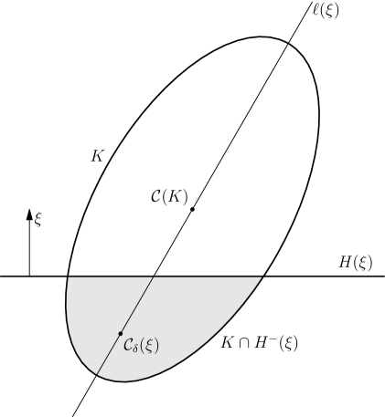
Figure 1. A body $K$, its submerged part $K\cap H^{-}(\xi)$ and the line $\ell(\xi)$ passing through ${\mathcal{C}}(K)$ and ${\mathcal{C}}_{\delta}(\xi)$.

Definition 2.

The geometric locus $\{{\mathcal{C}}_{\delta}(\xi):\,\xi\in S^{d-1}\}$ is called the surface of centers ${\mathcal{S}}={\mathcal{S}}_{\delta}$ or the surface of buoyancy.

Now we recall the notion of characteristic points of a family of hyperplanes (cf. [BG, pp. 107-110], [Wea, pp. 48-50], or [Za, pp. 26-54]).

Definition 3.

Let $d\geq 2$, $\xi_{0}\in S^{d-1}$, and let $\rho\in[-1,1)$. Consider a family ${\mathcal{Q}}$ of hyperplanes in ${\mathbb{R}^{d}}$ such that for every direction $\xi\in{\mathcal{B}}(\xi_{0},\rho)$ there exists a hyperplane in ${\mathcal{Q}}$ orthogonal to $\xi$. Assume also that for any $H\in{\mathcal{Q}}$, for any $(d-2)$-dimensional subspace $\Gamma$ parallel to $H$ and for any sequence $\{H_{k}\}_{k=1}^{\infty}$ of hyperplanes $H_{k}\in{\mathcal{Q}}$ converging to $H$ as $k\to\infty$ and parallel to $\Gamma$, the limit $\lim\limits_{k\to\infty}H\cap H_{k}$ exists. Given $H\in{\mathcal{Q}}$, we call a point $e\in H$ the characteristic point of ${\mathcal{Q}}$ with respect to $H$ if for any $\Gamma$ and $\{H_{k}\}_{k=1}^{\infty}$, as above, we have $e\in\lim\limits_{k\to\infty}H\cap H_{k}$.

We will need the following result from [O] (see the lemma on pp. 114-117 and Remark 1 on p. 117).

Theorem 3.

Let $d\geq 3$, let $K\subset{\mathbb{R}^{d}}$ be a convex body and let $\delta\in(0,\textnormal{vol}_{d}(K))$. The characteristic points of the family of cutting hyperplanes $\{H(\xi):\xi\in S^{d-1}\}$ for which (1) holds are the centers of mass of the sections $\{K\cap H(\xi):\,\xi\in S^{d-1}\}$.

Conversely, if the characteristic points of the family of hyperplanes $\{H(\xi):\,\xi\in S^{d-1}\}$ intersecting the interior of $K$ and corresponding to the sections $\{K\cap H(\xi):\,\xi\in S^{d-1}\}$ coincide with the centers of mass of these sections, then the function $\xi\mapsto\textnormal{vol}_{d}(K\cap H^{-}(\xi))$ is constant on $S^{d-1}$ and the constant is equal to some $\delta\in(0,\textnormal{vol}_{d}(K))$.

Since the reference [O] is not readily available, for convenience of the reader we present the proof of Theorem 3 in Appendix A.

To define the moments of inertia (see [Zh, p. 553]), consider a convex body $K$ and a hyperplane $H(\xi)$ for which (1) holds. Choose any $(d-2)$-dimensional plane $\Pi\subset H(\xi)$ passing through the center of mass ${\mathcal{C}}(K\cap H(\xi))$ and let $\eta_{1},\dots,\eta_{d-2},\eta_{d-1}$ be an orthonormal basis of $\xi^{\perp}=\{p\in{\mathbb{R}^{d}}:\,p\cdot\xi=0\}$ such that

(2) $$\Pi={\mathcal{C}}(K\cap H(\xi))+\textrm{span}(\eta_{1},\dots,\eta_{d-2}),\quad H(\xi)={\mathcal{C}}(K\cap H(\xi))+\xi^{\perp}.$$

Definition 4.

The moment of inertia $I_{K\cap H(\xi)}(\Pi)$ of $K\cap H(\xi)$ with respect to $\Pi$ is calculated by summing $\textnormal{dist}(\Pi,p)^{2}$ for every “particle” $p$ in the set $K\cap H(\xi)$, (see Figure 2), i.e.,

(3) $$I_{K\cap H(\xi)}(\Pi)=\int\limits_{K\cap H(\xi)}\textnormal{dist}(\Pi,p)^{2}dp=\int\limits_{K\cap H(\xi)-{\mathcal{C}}(K\cap H(\xi))}(q\cdot\eta_{d-1})^{2}\,dq,$$

where $\textnormal{dist}(\Pi,p)=\min\limits_{\{q\in\Pi\}}|p-q|$.

Figure 2. Two-dimensional body $K\cap H(\xi)$ with center of mass at the origin, and a line $\Pi$ parallel to $\eta_{1}$; we have $\textnormal{dist}(\Pi,q)^{2}=|q|^{2}-(q\cdot\eta_{1})^{2}=(q\cdot\eta_{2})^{2}$.

We will use the converse part of the following theorem (see [R, Theorem 1] or [FSWZ, Theorem 1.1]).

Theorem 4.

Let $d\geq 3$, let $K\subset{\mathbb{R}^{d}}$ be a convex body and let $\delta\in(0,\textnormal{vol}_{d}(K))$.

If $K$ floats in equilibrium at the level $\delta$ in every orientation, then for all $\xi\in S^{d-1}$ and for all $(d-2)$-dimensional planes $\Pi\subset H(\xi)$ passing through the center of mass ${\mathcal{C}}(K\cap H(\xi))$, the cutting sections $K\cap H(\xi)$ have equal moments of inertia independent of $\xi$ and $\Pi$.

Conversely, let ${\mathcal{C}}({\mathcal{S}})={\mathcal{C}}(K)$. If for all cutting hyperplanes $H(\xi)$, $\xi\in S^{d-1}$, and for all $(d-2)$-dimensional planes $\Pi\subset H(\xi)$ passing through the center of mass ${\mathcal{C}}(K\cap H(\xi))$, the cutting sections $K\cap H(\xi)$ have equal moments of inertia independent of $\xi$ and $\Pi$, then $K$ floats in equilibrium in every orientation at the level $\delta$.

For convenience of the reader we prove the converse part of this theorem in Appendix B.

Remark 1.

Let $\delta=\frac{\textnormal{vol}_{d}(K)}{2}$. Since for any $\xi\in S^{d-1}$, ${\mathcal{C}}(K)$ is the arithmetic average of ${\mathcal{C}}(K\cap H^{+}(\xi))$ and ${\mathcal{C}}(K\cap H^{-}(\xi))$, the condition ${\mathcal{C}}({\mathcal{S}})={\mathcal{C}}(K)$ is satisfied and ${\mathcal{S}}$ is symmetric with respect to ${\mathcal{C}}(K)$.

3. Reduction to a system of integral equations

Let $d\geq 3$. We follow the notation from [NRZ]. We will be dealing with bodies of revolution

$$K_{f}=\{x\in{\mathbb{R}^{d}}:\,x_{2}^{2}+x_{3}^{2}+\dots+x_{d}^{2}\leq f^{2}(x_{1})\}$$

obtained by the rotation of a smooth concave function supported on $[-R_{1},R_{2}]$ about the $x_{1}$-axis. Let $L(s,t)=L_{s}(t)=st+h(s)$ be a linear function with slope $s\in{\mathbb{R}}$, and let

$$H(L_{s})=\{x\in{\mathbb{R}^{d}}:\,x_{d}=L_{s}(x_{1})\}$$

be the corresponding hyperplane. The function $h$ will be chosen later. For now it is enough to assume that it is infinitely smooth, not identically zero, supported on $[1-2\tau,1-\tau]$ for some small $\tau>0$, and $h$ and sufficiently many of its derivatives are small. Let $-x=-x(s)$ and $y=y(s)$ be the first coordinates of the points of intersection of $\pm f$ and $L$ (see Figure 3).

Figure 3. Sections of $K_{f}$ and $H(L)$ by the $(x_{1},x_{d})$-plane.

To construct a system of two integral equations we will prove four lemmas. Consider the family of hyperplanes

(4) $${\mathcal{F}}=\{H(L_{s}):\,s\in[0,\infty)\}.$$

Lemma 1.

Let $E$ be the set of characteristic points of ${\mathcal{F}}$. Then,

(5) $$E=\{(-h^{\prime}(s),0,\dots,0,L(s,-h^{\prime}(s)))\in{\mathbb{R}^{d}}:\,s\in[0,\infty)\}.$$

Proof.

Let ${\mathcal{G}}$ be the family of lines ${\mathcal{G}}=\{\ell_{s}:\,s\in[0,\infty)\}$, where each line $\ell_{s}$ is the intersection of $H(L_{s})$ and the $x_{1}x_{d}$-plane. It is enough to show that

$$E\cap\{x_{1}x_{d}\!-\!\textnormal{plane}\}=\{(-h^{\prime}(s),-sh^{\prime}(s)+h(s))\in{\mathbb{R}^{2}}:\,s\in[0,\infty)\}.$$

We will use Definition 3. Let $s\in(1-2\tau,1-\tau)$ and let $\ell_{s}\in{\mathcal{G}}$. Choose any sequence $\{\ell_{s_{k}}\}_{k=1}^{\infty}$, $\ell_{s_{k}}\in{\mathcal{G}}$, converging to $\ell_{s}$ as $k\to\infty$, and let $\{u_{s_{k}}\}_{k=1}^{\infty}$, $\{u_{s_{k}}\}=\ell_{s}\cap\ell_{s_{k}}$, be the corresponding sequence of points of intersection. Solving the system of two linear equations we see that

$$u_{s_{k}}=\Big{(}\frac{h(s)-h(s_{k})}{s_{k}-s},s_{k}\frac{h(s)-h(s_{k})}{s_{k}-s}+h(s_{k})\Big{)}.$$

Hence, $\lim\limits_{s_{k}\to s}u_{s_{k}}$ exists and the point $\lim\limits_{s_{k}\to s}u_{s_{k}}=(-h^{\prime}(s),-sh(s)+h(s))$ is the characteristic point of ${\mathcal{G}}$ with respect to $\ell_{s}$.

Next, we observe that $(0,0)$ is the characteristic point of ${\mathcal{G}}$ with respect to $\ell_{1-2\tau}$. Indeed, it is enough to choose two sequences of lines in ${\mathcal{G}}$, $\{\ell_{s_{k}}\}_{k=1}^{\infty}$, $\{\ell_{s_{k}^{\prime}}\}_{k=1}^{\infty}$, both converging to $\ell_{1-2\tau}$, such that $s_{k}\in(1-2\tau,1-\tau)$ and $s_{k}^{\prime}\in(0,1-2\tau)$, and to use the fact that $\ell_{s_{k}^{\prime}}\cap\ell_{1-2\tau}=\{(0,0)\}$ for any line $\ell_{s_{k}^{\prime}}$ with $s_{k}^{\prime}\in(0,1-2\tau)$. Similarly, to show that $(0,0)$ is the characteristic point of ${\mathcal{G}}$ with respect to $\ell_{1-\tau}$, it is enough to choose the corresponding sequences $\{\ell_{s_{k}}\}_{k=1}^{\infty}$, $\{\ell_{s_{k}^{\prime\prime}}\}_{k=1}^{\infty}$, both converging to $\ell_{1-\tau}$, where $s_{k}\in(1-2\tau,1-\tau)$ and $s_{k}^{\prime\prime}\in(1-\tau,\infty)$.

To finish the proof, it remains to observe that since $h$ is supported by $[1-2\tau,1-\tau]$, any two lines $\ell_{s}$, $\ell_{s^{\prime}}$, $s,s^{\prime}\in[0,1-2\tau)\cup(1-\tau,\infty)$, intersect at $(0,0)$. Hence, $(0,0)$ is the characteristic point of ${\mathcal{G}}$ with respect to any line $\ell_{s}$ for $s\in[0,1-2\tau]\cup[1-\tau,\infty)$. ∎

Lemma 2.

Let $s>0$. The condition

(6) $${\mathcal{C}}(K_{f}\cap H(L_{s}))=(-h^{\prime}(s),0,\dots,0,L(s,-h^{\prime}(s)))$$

reads as

(7) $$\int\limits_{-x(s)}^{y(s)}(t+h^{\prime}(s))(f(t)^{2}-L(s,t)^{2})^{\frac{d-2}{2}}dt=0.$$

Let

$$\Pi_{1}=\{x\in H(L_{s}):\,x_{1}=-h^{\prime}(s)\},\qquad\quad\Pi_{j}=\{x\in H(L_{s}):\,x_{j}=0\},$$

$j=2,\dots,d-1$. The moments of inertia conditions

$$I_{j}=I_{K_{f}\cap H(L_{s})}(\Pi_{j})=const,\quad j=1,\dots,d-1,$$

read as

(8) $$I_{1}=\kappa_{d-2}(1+s^{2})^{\frac{3}{2}}\int\limits_{-x(s)}^{y(s)}(t+h^{\prime}(s))^{2}(f(t)^{2}-L(s,t)^{2})^{\frac{d-2}{2}}dt=const,$$

(9) $$I_{j}=\gamma_{d-2}\,\sqrt{1+s^{2}}\,\int\limits_{-x(s)}^{y(s)}(f(t)^{2}-L(s,t)^{2})^{\frac{d}{2}}dt=const,$$

where

$$\gamma_{d-2}=\int\limits_{B^{d-2}_{2}}p_{j}^{2}dp,\quad j=2,\dots,d-1.$$

Proof.

Fix $s>0$. Observe that the slice $K_{f}\cap H(L_{s})\cap H_{t}$ of the cutting section $K_{f}\cap H(L_{s})$ by the hyperplane $H_{t}=\{x\in{\mathbb{R}^{d}}:\,x_{1}=t\}$, $-x(s)<t<y(s)$, is the $(d-2)$-dimensional Euclidean ball

$$B_{2}^{d-2}((t,0,\dots,0,L(s,t)),r)\!=\!\{(t,x_{2},\dots,x_{d-1},L(s,t)):x_{2}^{2}+\dots+x_{d-1}^{2}\leq r^{2}\}$$

of radius $r=\sqrt{f^{2}(t)-L^{2}(s,t)}$ centered at $(t,0,\dots,0,L(s,t))$. Hence, for the first coordinate of the center of mass in (6) we have

(10) $$\int\limits_{-x(s)}^{y(s)}(t+h^{\prime}(s))dt\int\limits_{B_{2}^{d-2}((t,0,\dots,0,L(s,t)),r)}dp=$$

$$\kappa_{d-2}\int\limits_{-x(s)}^{y(s)}(t+h^{\prime}(s))(f(t)^{2}-L(s,t)^{2})^{\frac{d-2}{2}}dt=0.$$

This gives (7).

Similarly, since the distance in $K_{f}\cap H(L_{s})$ between the points $(t,x_{2},\dots,x_{d})$ $\in K_{f}\cap H(L_{s})\cap H_{t}$ and $(-h^{\prime}(s),x_{2},\dots,x_{d})\in K_{f}\cap H(L_{s})\cap H_{-h^{\prime}(s)}$ is $\sqrt{1+s^{2}}|t+h^{\prime}(s)|$, we have

$$I_{1}=\sqrt{1+s^{2}}\int\limits_{-x(s)}^{y(s)}(\sqrt{1+s^{2}}(t+h^{\prime}(s))^{2}dt\int\limits_{B_{2}^{d-2}((t,0,\dots,0,L(s,t)),r)}dp=$$

$$\kappa_{d-2}(1+s^{2})^{\frac{3}{2}}\int\limits_{-x(s)}^{y(s)}(t+h^{\prime}(s))^{2}(f(t)^{2}-L(s,t)^{2})^{\frac{d-2}{2}}dt,$$

proving (8). Finally, the expression in the left-hand side of (9) for the other moments can be obtained as

$$I_{j}=\sqrt{1+s^{2}}\int\limits_{-x(s)}^{y(s)}dt\int\limits_{B_{2}^{d-2}((t,0,\dots,0,L(s,t)),r)}p_{j}^{2}dp=$$

$$\sqrt{1+s^{2}}\,\gamma_{d-2}\,\int\limits_{-x(s)}^{y(s)}(f(t)^{2}-L(s,t)^{2})^{\frac{d}{2}}dt.$$

∎

Lemma 3.

Let $s_{o}\geq 0$, let $K_{f}$ be as above and let ${\mathcal{F}}$ be the family of hyperplanes defined as in (4) for $s\geq s_{0}$, so that (6) holds for $s\geq s_{o}$. Then for all $s>s_{o}$ and for all $(d-2)$-dimensional planes $\Pi\subset H(L_{s})$ passing through the center of mass ${\mathcal{C}}(K_{f}\cap H(L_{s}))$, the cutting sections $K_{f}\cap H(L_{s})$ have equal moments of inertia $I_{K_{f}\cap H(L_{s})}(\Pi)$ independent of $s$ and $\Pi$, provided (8) and (9) hold with the same constant on the right-hand side, which is independent of $s$ and $j=1,\dots,d-1$.

Proof.

Let $s_{o}\geq 0$ and let $s>s_{o}$ be fixed. If $\Pi\subset H(L_{s})$ is any $(d-2)$-dimensional plane passing through the center of mass ${\mathcal{C}}_{s}={\mathcal{C}}(K_{f}\cap H(L_{s}))$, then by (3) we have

$$I_{K_{f}\cap H(L_{s})}(\Pi)=\int\limits_{K_{f}\cap H(L_{s})}((u-{\mathcal{C}}_{s})\cdot\eta)^{2}\,du,$$

where $\eta=\eta_{d-1}$ is a unit vector in the hyperplane $H(L_{s})-{\mathcal{C}}_{s}$ which is orthogonal to $l$.

Let $\iota_{1},\dots\iota_{d-1}$ be the orthonormal basis in $H(L_{s})-{\mathcal{C}}_{s}$ such that $\iota_{1}\in\textrm{span}\{e_{1},e_{d}\}$ and $\iota_{j}=e_{j}$ for $j=2,\dots,d-1$. Decomposing $\eta$ in this basis as $\sum\limits_{j=1}^{d-1}{\eta}_{(j)}\iota_{j}$, we have

$$I_{K_{f}\cap H(L_{s})}(\Pi)=\sum\limits_{j=1}^{d-1}\eta_{(j)}^{2}\int\limits_{K_{f}\cap H(L_{s})}((u-{\mathcal{C}}_{s})\cdot\iota_{j})^{2}\,du\,+$$

$$\sum\limits_{{\begin{subarray}{c}j,l=1\\ j\neq l\end{subarray}}}^{d-1}\eta_{(j)}\eta_{(l)}\int\limits_{K_{f}\cap H(L_{s})}((u-{\mathcal{C}}_{s})\cdot\iota_{j})((u-{\mathcal{C}}_{s})\cdot\iota_{l})\,du=J_{1}+J_{2}.$$

Using the fact that $\eta$ is a unit vector, together with (8) and (9), we have that $J_{1}$ is constant.

We claim that $J_{2}=0$. Indeed, if $j$ is equal to $1$, then arguing as in the previous lemma, and using the fact that $\int\limits_{B^{d-2}_{2}}p_{l}dp=0$ for $l=2,\dots,d-1$, we see that

$$\int\limits_{K_{f}\cap H(L_{s})}((u-{\mathcal{C}}_{s})\cdot\iota_{1})((u-{\mathcal{C}}_{s})\cdot\iota_{l})\,du=$$

$$\sqrt{1+s^{2}}\int\limits_{-x(s)}^{y(s)}(t+h^{\prime}(s))dt\int\limits_{B_{2}^{d-2}((t,0,\dots,0,L(s,t)),r)}p_{l}dp=0.$$

The case when $l=1$ is similar.

If $j\neq 1$, $l\neq 1$, then we use the fact that $\int\limits_{B^{d-2}_{2}}p_{j}p_{l}dp=0$ for $j,l=2,\dots,d-1$, $j\neq l$, to obtain

$$\int\limits_{K_{f}\cap H(L_{s})}((u-{\mathcal{C}}_{s})\cdot\iota_{j})((u-{\mathcal{C}}_{s})\cdot\iota_{l})\,du=\int\limits_{-x(s)}^{y(s)}dt\int\limits_{B_{2}^{d-2}((t,0,\dots,0,L(s,t)),r)}p_{j}p_{l}dp=0.$$

Thus, $I_{K_{f}\cap H(L_{s})}(\Pi)$ is a constant independent of $s$ and of the arbitrarily chosen $\Pi$. The lemma is proved. ∎

Lemma 4.

Let $s_{o}\geq 0$. Assume that (7) is valid for all $s>s_{o}$. Then (9) holds for all $s>s_{o}$ with the constant independent of $s$ if and only if (8) holds for all $s>s_{o}$ with the constant independent of $s$.

Proof.

We recall that

(11) $$\,\,\,L(s,t)=st+h(s),\quad f(y(s))=L(s,y(s)),\quad f(-x(s))=L(s,-x(s)),$$

for $s\in{\mathbb{R}}$. Let $s_{o}\geq 0$ and let $s>s_{o}$. We rewrite (9) as

$$\int\limits_{-x(s)}^{y(s)}(f(t)^{2}-L(s,t)^{2})^{\frac{d}{2}}dt=\frac{const}{\gamma_{d-2}\,\sqrt{1+s^{2}}}$$

and differentiate both sides with respect to $s$ using (11). We have

$$\int\limits_{-x(s)}^{y(s)}(f(t)^{2}-L(s,t)^{2})^{\frac{d-2}{2}}(st+h(s))(t+h^{\prime}(s))dt=\frac{const\,\,s}{d\gamma_{d-2}\,(1+s^{2})^{\frac{3}{2}}}.$$

Adding and subtracting $sh^{\prime}(s)$ in the second parentheses under the integral and using (7), the last equality yields

$$s\,\int\limits_{-x(s)}^{y(s)}(f(t)^{2}-L(s,t)^{2})^{\frac{d-2}{2}}(t+h^{\prime}(s))^{2}dt=\frac{const\,\,s}{d\gamma_{d-2}\,(1+s^{2})^{\frac{3}{2}}}.$$

Canceling $s$ and passing to polar coordinates,

$$d\gamma_{d-2}=\frac{d}{d-2}\int\limits_{B^{d-2}_{2}}|p|^{2}dp=\frac{d}{d-2}\int\limits_{S^{d-3}}d\omega\int\limits_{0}^{1}r^{2+d-3}dr=\frac{\omega(S^{d-3})}{d-2}=\kappa_{d-2},$$

where $\omega(S^{d-3})$ is the surface area of $S^{d-3}$, we have (8).

Now we prove the converse statement. Fix any $j=2,\dots,d-1$. We rewrite the first equality in (9) as

$$\frac{I_{j}(s)}{\gamma_{d-2}\,\sqrt{1+s^{2}}}=\int\limits_{-x(s)}^{y(s)}(f(t)^{2}-L(s,t)^{2})^{\frac{d}{2}}dt$$

and differentiate both sides with respect to $s$. Using (7) and (8), we see that

(12) $$\Big{(}\frac{I_{j}(s)}{\sqrt{1+s^{2}}}\Big{)}^{\prime}=\frac{I_{j}^{\prime}(s)(1+s^{2})-sI_{j}(s)}{(1+s^{2})^{\frac{3}{2}}}=-\frac{const\,\,s}{(1+s^{2})^{\frac{3}{2}}},$$

where the second equality above is obtained follows. Using (11) we differentiate the first equality in (9) to obtain

$$I_{j}^{\prime}(s)(1+s^{2})=\gamma_{d-2}\,s\sqrt{1+s^{2}}\int\limits_{-x(s)}^{y(s)}(f(t)^{2}-L(s,t)^{2})^{\frac{d}{2}}dt-$$

$$d\gamma_{d-2}(1+s^{2})^{\frac{3}{2}}\int\limits_{-x(s)}^{y(s)}(f(t)^{2}-L(s,t)^{2})^{\frac{d-2}{2}}(st+h(s))(t+h^{\prime}(s))dt.$$

Adding and subtracting $sh^{\prime}(s)$ in the second parentheses under the second integral and using (7), the fact that $d\gamma_{d-2}=\kappa_{d-2}$ and the second equality in (8), we have

$$I_{j}^{\prime}(s)(1+s^{2})-sI_{j}(s)=sI_{j}(s)-sI_{1}-sI_{j}(s)=-sI_{1}=-const\,s.$$

This gives the second equality in (12), i.e.,

$$I_{j}^{\prime}(s)-\frac{s}{1+s^{2}}I_{j}(s)+const\frac{s}{1+s^{2}}=0.$$

Solving this linear ODE with an integrating factor $\frac{1}{\sqrt{1+s^{2}}}$, we have

$$I_{j}(s)=\sqrt{1+s^{2}}\Big{(}\frac{const}{\sqrt{1+s^{2}}}+c_{1}\Big{)}=const+c_{1}\,\sqrt{1+s^{2}}$$

with some constant $c_{1}$. Since $I_{j}$ is bounded on $[s_{o},\infty)$, $c_{1}=0$, and we obtain the converse part of the lemma. ∎

Let

(13) $$f_{o}(t)=\sqrt{1-t^{2}},\qquad L_{o}(s,t)=st,\qquad x_{o}(s)=y_{o}(s)=\frac{1}{\sqrt{1+s^{2}}},$$

where $f_{o}$ describes the boundary of the unit Euclidean ball, $L_{o}$ corresponds to the linear subspace passing through the origin with $h\equiv 0$, and $x_{o}$, $y_{o}$ are the first coordinates of the points of intersection of $\pm f$ and $L_{o}$. Our goal is to prove the following proposition.

Proposition 1.

Let $n=\frac{d}{2}$. A body $K_{f}$ floats in equilibrium in every orientation at the level $\frac{\textnormal{vol}_{d}(K)}{2}$, provided for all $s>0$,

(14) $$\int\limits_{-x(s)}^{y(s)}(f(t)^{2}-L(s,t)^{2})^{n}dt=\int\limits_{-x_{o}(s)}^{y_{o}(s)}(f_{o}(t)^{2}-L_{o}(s,t)^{2})^{n}dt=\frac{const}{\sqrt{1+s^{2}}},$$

(15) $$\int\limits_{-x(s)}^{y(s)}(f(t)^{2}-L(s,t)^{2})^{n-1}\frac{\partial L(s,t)}{\partial s}\,dt=0.$$

We remark that (14) and (15) are similar to equations (4) and (5) from [NRZ].

Proof.

Observe that $H(L_{0})$ divides $K_{f}$ into two parts of equal volume. Also, (15) is the same as (7) of Lemma 2. Thus, by Lemma 1 and Lemma 2 the characteristic points of the family of hyperplanes $\{H(L_{s})$, $s\in[0,\infty)\}$, are exactly the centers of mass of the sections $K\cap H(L_{s})$. Hence, we can apply the converse part of Theorem 3 to conclude that they are the cutting hyperplanes at the level $\frac{\textrm{vol}_{d}(K)}{2}$.

On the other hand, observing that conditions (14), (15) are the same as (9) and (7), by Lemma 4 condition (8) also holds. Therefore, by Lemma 3, the cutting sections have equal moments of inertia for all $(d-2)$-dimensional planes passing through the centers of mass of these sections. By Remark 1, all conditions of the converse part of Theorem 4 are satisfied, and the proposition follows. ∎

In order to construct a counterexample, we will choose the perturbation function $h$ with the properties described at the beginning of this section. The convex body corresponding to any such function will automatically be asymmetric since not all its sections dividing the volume in half will pass through a single point.

4. The case of even $d\geq 4$

Note that in this case $n=\frac{d}{2}\in{\mathbb{N}}$. Our argument is very similar to the one in Section 3 of [NRZ]. Our body $K_{f}$ will be a local perturbation of the Euclidean ball, i.e., the resulting function $f(t)$ will be equal to $\sqrt{1-t^{2}}$ everywhere on $[-1,1]$ except $[-\frac{1}{\sqrt{1+(1-2\tau)^{2}}},-\frac{1}{\sqrt{1+(1-\tau)^{2}}}]\cup[\frac{1}{\sqrt{1+(1-\tau)^{2}}},\frac{1}{\sqrt{1+(1-2\tau)^{2}}}]$ for some small $\tau>0$.

Equations (11) show that to define $f$, it is enough to define two decreasing functions $x(s)$, $y(s)$ on $[0,+\infty)$. Our functions $x(s)$ and $y(s)$ will coincide with $x_{o}$ and $y_{o}$ for all $s\notin[1-2\tau,1-\tau]$, where $x_{o}$, $y_{o}$ are defined by (13). Since the curvature of the semicircle is strictly positive, the resulting function $f$ will be strictly concave if $x$ and $y$ are close to $x_{o}$ and $y_{o}$ in $C^{2}$.

We will make our construction in several steps. First, we define $x=x_{o}$, $y=y_{o}$ on $[1,\infty)$. Second, we will express equations (14), (15) purely in terms of $x$ and $y$ (see (18) and (19) below). Then we will use these new equations to extend the functions $x$ and $y$ to $[1-3\tau,1]$. We will be able to do it if $\tau$ and $h$ are sufficiently small. Moreover, the extensions will coincide with $x_{o}$ and $y_{o}$ on $[1-\tau,1]$ and will be close to $x_{o}$ and $y_{o}$ up to two derivatives on $[1-3\tau,1-\tau]$. Then, we will show that our extensions automatically coincide with $x_{o}$ and $y_{o}$ on $[1-3\tau,1-2\tau]$ as well. This will allow us to put $x=x_{o}$, $y=y_{o}$ on the remaining interval $[0,1-3\tau]$ and get a nice smooth function. Finally, we will show that equations (14), (15) will be satisfied up to $s=0$, thus finishing the proof.

Step 1. We put $x=x_{o}$, $y=y_{o}$ on $[1,\infty)$.

Step 2. To construct $x$, $y$ on $[1-3\tau,1]$, we will make some technical preparations. First, we will differentiate equations (14), (15) a few times to obtain a system of four integral equations with four unknown functions $x$, $y$, $x^{\prime}$, $y^{\prime}$. Next, we will apply Lemma 8 and Remark 2 from [NRZ, pp. 63-66] to show that there exists a solution $x$, $y$, $x^{\prime}$, $y^{\prime}$ of the constructed system of integral equations on $[1-3\tau,1]$, which coincides with $x_{o}$, $y_{o}$, $\frac{dx_{o}}{ds}$, $\frac{dy_{o}}{ds}$ on $[1-\tau,1]$. Finally, we will prove that the $x$ and $y$ components of that solution give a solution of (14), (15) with $f$ defined by (11).

Differentiating equation (14) $n+1$ times and equation (15) $n$ times with respect to $s$ and using (11), we obtain

$$(-2)^{n}n!\Big{[}\Big{(}\Big{(}L\frac{\partial L}{\partial s}\Big{)}\Big{|}_{(s,-x(s))}\Big{)}^{n}\frac{dx}{ds}(s)\,+\Big{(}\Big{(}L\frac{\partial L}{\partial s}\Big{)}\Big{|}_{(s,y(s))}\Big{)}^{n}\frac{dy}{ds}(s)\Big{]}\,+$$

(16) $$\int\limits_{-x(s)}^{y(s)}\Big{(}\frac{\partial}{\partial s}\Big{)}^{n+1}\Big{(}(f(t)^{2}-L(s,t)^{2})^{n}\Big{)}dt\,=\Big{(}\frac{d}{ds}\Big{)}^{n+1}\Big{(}\frac{const}{\sqrt{1+s^{2}}}\Big{)},$$

and

$$(-2)^{n-1}(n-1)!\Big{[}\Big{(}\Big{(}L\frac{\partial L}{\partial s}\Big{)}^{n-1}\frac{\partial L}{\partial s}\Big{)}\Big{|}_{(s,-x(s))}\frac{dx}{ds}(s)\,+\qquad\qquad\qquad$$

$$\qquad\qquad\qquad\qquad\qquad\qquad\qquad\qquad\Big{(}\Big{(}L\frac{\partial L}{\partial s}\Big{)}^{n-1}\frac{\partial L}{\partial s}\Big{)}\Big{|}_{(s,y(s))}\frac{dy}{ds}(s)\Big{]}\,+$$

(17) $$\int\limits_{-x(s)}^{y(s)}\Big{(}\frac{\partial}{\partial s}\Big{)}^{n}\Big{(}(f(t)^{2}-L(s,t)^{2})^{n-1}\frac{\partial L}{\partial s}(s,t)\Big{)}dt=0.$$

When $s\leq 1$, the integral term $I$ in (16) can be split as

$$I=\int\limits_{-x(s)}^{y(s)}\Big{(}\frac{\partial}{\partial s}\Big{)}^{n+1}\Big{(}(f(t)^{2}-L(s,t)^{2})^{n}\Big{)}dt=$$

$$\Big{(}\int\limits_{-x(s)}^{-x_{o}(1)}\,+\,\int\limits_{y_{o}(1)}^{y(s)}\Big{)}\,\Big{(}\frac{\partial}{\partial s}\Big{)}^{n+1}\Big{(}(f(t)^{2}-L(s,t)^{2})^{n}\Big{)}dt\,+\,\Xi_{1}(s),$$

where

$$\Xi_{1}(s)=\int\limits^{y_{o}(1)}_{-x_{o}(1)}\Big{(}\frac{\partial}{\partial s}\Big{)}^{n+1}\Big{(}(f_{o}(t)^{2}-L(s,t)^{2})^{n}\Big{)}dt.$$

Making the change of variables $t=-x(\sigma)$ in the integral $\int_{-x(s)}^{-x_{o}(1)}$ and $t=y(\sigma)$ in the integral $\int_{y_{o}(1)}^{y(s)}$ and using (11), we obtain

$$I=-\int\limits_{s}^{1}\Big{(}\frac{\partial}{\partial s}\Big{)}^{n+1}\Big{(}L(\sigma,-x(\sigma))^{2}-L(s,-x(\sigma))^{2}\Big{)}^{n}\,\frac{dx}{ds}(\sigma)d\sigma\,-$$

$$\int\limits_{s}^{1}\Big{(}\frac{\partial}{\partial s}\Big{)}^{n+1}\Big{(}L(\sigma,y(\sigma))^{2}-L(s,y(\sigma))^{2}\Big{)}^{n}\,\frac{dy}{ds}(\sigma)d\sigma\,+\,\Xi_{1}(s).$$

Similarly, we have

$$\int\limits_{-x(s)}^{y(s)}\Big{(}\frac{\partial}{\partial s}\Big{)}^{n}\Big{(}(f(t)^{2}-L(s,t)^{2})^{n-1}\frac{\partial L}{\partial s}(s,t)\Big{)}dt=$$

$$-\int\limits_{s}^{1}\Big{(}\frac{\partial}{\partial s}\Big{)}^{n}\Big{(}\Big{(}L(\sigma,-x(\sigma))^{2}-L(s,-x(\sigma))^{2}\Big{)}^{n-1}\frac{\partial L}{\partial s}(s,-x(\sigma))\Big{)}\,\frac{dx}{ds}(\sigma)d\sigma\,-$$

$$\int\limits_{s}^{1}\Big{(}\frac{\partial}{\partial s}\Big{)}^{n}\Big{(}\Big{(}L(\sigma,y(\sigma))^{2}-L(s,y(\sigma))^{2}\Big{)}^{n-1}\frac{\partial L}{\partial s}(s,y(\sigma))\Big{)}\,\frac{dy}{ds}(\sigma)d\sigma\,+\,\Xi_{2}(s),$$

where

$$\Xi_{2}(s)=\int\limits^{y_{o}(1)}_{-x_{o}(1)}\Big{(}\frac{\partial}{\partial s}\Big{)}^{n}\Big{(}(f_{o}(t)^{2}-L(s,t)^{2})^{n-1}\frac{\partial L}{\partial s}(s,t)\Big{)}dt.$$

To reduce the resulting system of integro-differential equations to a pure system of integral equations we add two independent unknown functions $x^{\prime}$, $y^{\prime}$ and two new relations:

$$x(s)=-\int\limits_{s}^{1}x^{\prime}(\sigma)d\sigma+x_{o}(1),\qquad y(s)=-\int\limits_{s}^{1}y^{\prime}(\sigma)d\sigma+y_{o}(1).$$

We rewrite our equations (16), (17) as follows:

(18) $$(-2)^{n}n!\Big{[}\Big{(}\Big{(}L\frac{\partial L}{\partial s}\Big{)}\Big{|}_{(s,-x(s))}\Big{)}^{n}x^{\prime}(s)\,+\Big{(}\Big{(}L\frac{\partial L}{\partial s}\Big{)}\Big{|}_{(s,y(s))}\Big{)}^{n}y^{\prime}(s)\Big{]}\,-$$

$$\int\limits_{s}^{1}\Big{(}\frac{\partial}{\partial s}\Big{)}^{n+1}\Big{(}L(\sigma,-x(\sigma))^{2}-L(s,-x(\sigma))^{2}\Big{)}^{n}\,x^{\prime}(\sigma)d\sigma\,-$$

$$\int\limits_{s}^{1}\Big{(}\frac{\partial}{\partial s}\Big{)}^{n+1}\Big{(}L(\sigma,y(\sigma))^{2}-L(s,y(\sigma))^{2}\Big{)}^{n}\,y^{\prime}(\sigma)d\sigma\,+\,\Xi_{1}(s)=$$

$$\Big{(}\frac{d}{ds}\Big{)}^{n+1}\Big{(}\frac{const}{\sqrt{1+s^{2}}}\Big{)},$$

and

(19) $$(-2)^{n-1}(n-1)!\Big{[}\Big{(}\Big{(}L\frac{\partial L}{\partial s}\Big{)}^{n-1}\frac{\partial L}{\partial s}\Big{)}\Big{|}_{(s,-x(s))}x^{\prime}(s)\,+\qquad\qquad\qquad$$

$$\qquad\qquad\qquad\qquad\qquad\qquad\qquad\qquad\Big{(}\Big{(}L\frac{\partial L}{\partial s}\Big{)}^{n-1}\frac{\partial L}{\partial s}\Big{)}\Big{|}_{(s,y(s))}y^{\prime}(s)\Big{]}\,-$$

$$\int\limits_{s}^{1}\Big{(}\frac{\partial}{\partial s}\Big{)}^{n}\Big{(}\Big{(}L(\sigma,-x(\sigma))^{2}-L(s,-x(\sigma))^{2}\Big{)}^{n-1}\frac{\partial L}{\partial s}(s,-x(\sigma))\Big{)}\,x^{\prime}(\sigma)d\sigma\,-$$

$$\int\limits_{s}^{1}\Big{(}\frac{\partial}{\partial s}\Big{)}^{n}\Big{(}\Big{(}L(\sigma,y(\sigma))^{2}-L(s,y(\sigma))^{2}\Big{)}^{n-1}\frac{\partial L}{\partial s}(s,y(\sigma))\Big{)}\,y^{\prime}(\sigma)d\sigma+\Xi_{2}(s)=0.$$

Now we rewrite our system in the form

(20) $$\mathbf{G}(s,Z(s))=\int\limits_{s}^{1}\mathbf{\Theta}(s,\sigma,Z(\sigma))d\sigma+\mathbf{\Xi}(s).$$

Here

$$Z=\left(\begin{array}[]{cccc}x\\ y\\ x^{\prime}\\ y^{\prime}\end{array}\right),$$

$$\mathbf{G}(s,Z)=\left(\begin{array}[]{cccc}x\\ y\\[7.0pt] (-2)^{n}n!\Big{[}\Big{(}L\frac{\partial L}{\partial s}\Big{|}_{(s,-x)}\Big{)}^{n}x^{\prime}\,+\Big{(}L\frac{\partial L}{\partial s}\Big{|}_{(s,y)}\Big{)}^{n}y^{\prime}\Big{]}\\[15.0pt] (-2)^{n-1}(n-1)!\Big{[}\Big{(}\Big{(}L\frac{\partial L}{\partial s}\Big{)}^{n-1}\frac{\partial L}{\partial s}\Big{)}\Big{|}_{(s,-x)}x^{\prime}\,+\Big{(}\Big{(}L\frac{\partial L}{\partial s}\Big{)}^{n-1}\frac{\partial L}{\partial s}\Big{)}\Big{|}_{(s,y)}y^{\prime}\Big{]}\\ \end{array}\right),$$

$$\mathbf{\Theta}(s,\sigma,Z)=-\left(\begin{array}[]{cccc}x^{\prime}\\ y^{\prime}\\ \Theta_{1}\\ \Theta_{2}\end{array}\right),$$

where

$$\Theta_{1}=-\Big{(}\frac{\partial}{\partial s}\Big{)}^{n+1}\Big{(}L(\sigma,-x)^{2}-L(s,-x)^{2}\Big{)}^{n}\,x^{\prime}\,-\Big{(}\frac{\partial}{\partial s}\Big{)}^{n+1}\Big{(}L(\sigma,y)^{2}-L(s,y)^{2}\Big{)}^{n}\,y^{\prime}\,,$$

$$\Theta_{2}=-\Big{(}\frac{\partial}{\partial s}\Big{)}^{n}\Big{(}\Big{(}L(\sigma,-x)^{2}-L(s,-x)^{2}\Big{)}^{n-1}\frac{\partial L}{\partial s}(s,-x)\Big{)}\,x^{\prime}\,-\qquad\qquad$$

$$\qquad\qquad\qquad\qquad\qquad\qquad\qquad\Big{(}\frac{\partial}{\partial s}\Big{)}^{n}\Big{(}\Big{(}L(\sigma,y)^{2}-L(s,y)^{2}\Big{)}^{n-1}\frac{\partial L}{\partial s}(s,y)\Big{)}\,y^{\prime},$$

and

$$\mathbf{\Xi}(s)=\left(\begin{array}[]{cccc}x_{o}(1)\\ y_{o}(1)\\ -\Xi_{1}(s)+\Big{(}\frac{d}{ds}\Big{)}^{n+1}\Big{(}\frac{const}{\sqrt{1+s^{2}}}\Big{)}\\ -\Xi_{2}(s)\end{array}\right).$$

Note that ${\mathbf{G}}$, ${\mathbf{\Theta}}$, ${\mathbf{\Xi}}$ are well defined and infinitely smooth for all $s,\sigma\in(0,1]$ and $Z\in{\mathbb{R}}^{4}$. Observe also that

$$D_{Z}{\mathbf{G}}\Big{|}_{(s,Z)}=\left(\begin{array}[]{cc}\mathbf{I}&0\\ \mathbf{*}&\mathbf{A}\\ \end{array}\right),$$

where

$${\mathbf{I}}=\left(\begin{array}[]{ccc}1&0\\ 0&1\end{array}\right),\qquad{\mathbf{A}}={\mathbf{A}(s,x,y)}=$$

$$\left(\begin{array}[]{ccc}(-2)^{n}n!\Big{(}\Big{(}L\frac{\partial L}{\partial s}\Big{)}\Big{|}_{(s,-x)}\Big{)}^{n}&(-2)^{n}n!\Big{(}\Big{(}L\frac{\partial L}{\partial s}\Big{)}\Big{|}_{(s,y)}\Big{)}^{n}\\ (-2)^{n-1}(n-1)!\Big{(}\Big{(}L\frac{\partial L}{\partial s}\Big{)}^{n-1}\frac{\partial L}{\partial s}\Big{)}\Big{|}_{(s,-x)}&(-2)^{n-1}(n-1)!\Big{(}\Big{(}L\frac{\partial L}{\partial s}\Big{)}^{n-1}\frac{\partial L}{\partial s}\Big{)}\Big{|}_{(s,y)}\end{array}\right).$$

The function

$$Z_{o}(s)=\left(\begin{array}[]{cccc}x_{o}(s)\\ y_{o}(s)\\[3.0pt] \frac{dx_{o}}{ds}(s)\\[3.0pt] \frac{dy_{o}}{ds}(s)\end{array}\right)$$

solves the system (20) with ${\mathbf{G}}$, ${\mathbf{\Theta}}$, ${\mathbf{\Xi}}$ corresponding to $h\equiv 0$ (we will denote them by ${\mathbf{G}_{o}}$, ${\mathbf{\Theta}_{o}}$, ${\mathbf{\Xi}_{o}}$) on $[\frac{1}{2},1]$.

We claim that

(21) $$\det\,\Big{(}D_{Z}{\mathbf{G}_{o}}\Big{|}_{(s,Z_{o}(s))}\Big{)}=\det({\mathbf{A}_{o}(s,x_{o}(s),y_{o}(s))})\neq 0\qquad\forall s\in(0,1].$$

Indeed, since the matrix ${\mathbf{A}_{o}}(s,x_{o}(s),y_{o}(s))$ is of the form

$$\left(\begin{array}[]{ccc}(-2)^{n}n!(sx_{o}(s))^{n}&(-2)^{n}n!(sy_{o}(s))^{n}\\ (-2)^{n-1}(n-1)!(sx_{o}(s))^{n-1}(-x_{o}(s))&(-2)^{n-1}(n-1)!(sy_{o}(s))^{n-1}y_{o}(s)\end{array}\right),$$

its sign pattern is

$$\left(\begin{array}[]{ccc}+&+\\ +&-\end{array}\right),\qquad\textrm{when}\,\,n\,\,\textrm{ is even},\quad\textrm{and }\qquad\left(\begin{array}[]{ccc}-&-\\ -&+\end{array}\right),\quad\textrm{when}\,n\,\,\textrm{ is odd}.$$

Thus, (21) follows. In particular,

$$\det\,\Big{(}D_{Z}{\mathbf{G}_{o}}\Big{|}_{(1,Z_{o}(1))}\Big{)}\neq 0.$$

Lemma 8 from [NRZ, p. 63] then implies that we can choose some small $\tau>0$ and, for any fixed $k\in{\mathbb{N}}$, construct a solution $Z(s)$ of (20) which is $C^{k}$-close to $Z_{o}(s)$ on $[1-3\tau,1]$, whenever ${\mathbf{G}}$, ${\mathbf{\Theta}}$, ${\mathbf{\Xi}}$ are sufficiently close to ${\mathbf{G}_{o}}$, ${\mathbf{\Theta}_{o}}$, ${\mathbf{\Xi}_{o}}$ in $C^{k}$ on certain compact sets. Since $\mathbf{G}$, $\mathbf{\Theta}$, $\mathbf{\Xi}$ and their derivatives are some explicit (integrals of) polynomials in $Z$, $s$, $\sigma$, $h(s)$, and the derivatives of $h(s)$, this closeness condition will hold if $h$ and sufficiently many of its derivatives are close enough to zero. Moreover, since $h$ vanishes on $[1-\tau,1]$, the assumptions of Remark 2 from [NRZ, p. 66] are satisfied and we have $Z(s)=Z_{o}(s)$ on $[1-\tau,1]$.

To prove that the $x$ and $y$ components of the solution we found give a solution of (14), (15) with $f$ defined by (11), we consider the functions

$$F(s):=\int\limits_{-x(s)}^{y(s)}\Big{(}f(s,t)^{2}-L(s,t)^{2}\Big{)}^{n}dt-\frac{const}{\sqrt{1+s^{2}}},$$

$$H(s):=\int\limits_{-x(s)}^{y(s)}\Big{(}f(s,t)^{2}-L(s,t)^{2}\Big{)}^{n-1}\frac{\partial L}{\partial s}(s,t)dt.$$

Since equations (18) and (19) of our system (20) were obtained by the differentiation of equations (14), (15), we have

$$\Big{(}\frac{d}{ds}\Big{)}^{n+1}F(s)=0,\qquad\Big{(}\frac{d}{ds}\Big{)}^{n}H(s)=0$$

on $[1-3\tau,1]$. Hence, $F$ and $H$ are polynomials on $[1-3\tau,1]$. Since $h(s)=0$, $x(s)=x_{o}(s)$, $y(s)=y_{o}(s)$ on $[1-\tau,1]$, $F$ and $H$ vanish on $[1-\tau,1]$ and, therefore, identically. Thus, we conclude that the $x$ and $y$ components of the solutions of (18), (19) solve (14), (15) on $(1-3\tau,1]$. Step 2 is completed.

Step 3. We claim that $x=x_{o}$, $y=y_{o}$ on $[1-3\tau,1-2\tau]$, i.e., the perturbed solution returns to the semicircle. Since $h$ is supported on $[1-2\tau,1-\tau]$, we have $L=L_{o}=st$ and $\frac{\partial}{\partial s}L(s,t)=t$ for $s\in[1-3\tau,1-2\tau]$. It follows that every time we differentiate equation (14) (with respect to $s$) we can divide the result by $s$ to obtain

(22) $$\int\limits_{-x(s)}^{y(s)}(f(t)^{2}-L_{o}(s,t)^{2})^{n-k}t^{2k}dt=\int\limits_{-x_{o}(s)}^{y_{o}(s)}(f_{o}(t)^{2}-L_{o}(s,t)^{2})^{n-k}t^{2k}dt,$$

for $k\leq n$. If we take $k=n$ in (22), we get

(23) $$\int\limits_{-x(s)}^{y(s)}t^{2n}dt=\int\limits_{-x_{o}(s)}^{y_{o}(s)}t^{2n}dt.$$

Similarly, for $k\leq n-1$, equation (15) implies that

(24) $$\int\limits_{-x(s)}^{y(s)}(f(t)^{2}-L_{o}(s,t)^{2})^{n-1-k}t^{2k+1}dt=\quad\qquad\qquad\qquad\qquad\qquad\qquad$$

$$\qquad\qquad\qquad\qquad\qquad\qquad\int\limits_{-x(s)}^{y(s)}(f(t)^{2}-L_{o}(s,t)^{2})^{n-1-k}t^{2k+1}dt=0.$$

Putting $k=n-1$ in (24), we get

(25) $$\int\limits_{-x(s)}^{y(s)}t^{2n-1}dt=0=\int\limits_{-x_{o}(s)}^{y_{o}(s)}t^{2n-1}dt.$$

Equation (25) yields $x(s)=y(s)$, and the symmetry (with respect to $0$) of the intervals $(-x_{o}(s),y_{o}(s))$, $(-x(s),y(s))$, together with (23), yield $(-x_{o}(s),y_{o}(s))$ $=(-x(s),y(s))$ for all $s\in[1-3\tau,1-2\tau]$. Step 3 is completed.

Step 4. We put $x=x_{o}$, $y=y_{o}$ on $[0,1-3\tau]$, which will result in a function $f$ defined on $[-1,1]$ and coinciding with $f_{o}(t)=\sqrt{1-t^{2}}$ outside small intervals around $\pm\frac{1}{\sqrt{2}}$. It remains to check that (14), (15) are valid for $s\in[0,1-3\tau]$. We will prove the validity of (15). The proof for equation (14) is similar and can be found in [NRZ, p. 53].

Since $h\equiv 0$ away from $(1-2\tau,1-\tau)$, we have $L(s,t)=st$ for $s\in[0,1-3\tau]$, so we need to check that

$$\int\limits_{-x(s)}^{y(s)}(f(t)^{2}-(st)^{2})^{n-1}\,tdt=\int\limits_{-x(s)}^{y(s)}(f_{o}(t)^{2}-(st)^{2})^{n-1}\,tdt,\qquad\forall s\in[0,1-3\tau].$$

Recall that $x=x_{o}$ and $y=y_{o}$ everywhere on this interval, so we can write $x$ and $y$ instead of $x_{o}$ and $y_{o}$ on the right-hand side.

Using the binomial formula, we see that it suffices to check that

(26) $$\int\limits_{-x(s)}^{y(s)}f(t)^{2j}\,t^{2(n-1-j)+1}dt=\int\limits_{-x(s)}^{y(s)}f_{o}(t)^{2j}\,t^{2(n-1-j)+1}dt,$$

$\forall j=1,\dots,n-1$ and $s\in[0,1-3\tau]$. Since $f\equiv f_{o}$ outside $[-x(1-3\tau),y(1-3\tau)]$, splitting the integrals in (26) into three parts with ranges $[-x(s),-x(1-3\tau)]$, $[-x(1-3\tau),y(1-3\tau)]$, $[y(1-3\tau),y(s)]$, it is enough to check (26) on the middle interval $[-x(1-3\tau),y(1-3\tau)]$.

To this end, we first take $s=1-3\tau$, $k=n-2$ in (24) and conclude that

(27) $$\int\limits_{-x(1-3\tau)}^{y(1-3\tau)}f(t)^{2}\,t^{2n-3}dt=\int\limits_{-x(1-3\tau)}^{y(1-3\tau)}f_{o}(t)^{2}\,t^{2n-3}dt,$$

which is (26) for $j=1$ and $s=1-3\tau$. Now we go “one step up”, by taking $s=1-3\tau$, $k=n-3$ in (24), to get

$$\int\limits_{-x(1-3\tau)}^{y(1-3\tau)}(f(t)^{2}-(st)^{2})^{2}t^{2n-5}dt=\int\limits_{-x(1-3\tau)}^{y(1-3\tau)}(f_{o}(t)^{2}-(st)^{2})^{2}t^{2n-5}dt.$$

The last equality together with (27) yield

$$\int\limits_{-x(1-3\tau)}^{y(1-3\tau)}f(t)^{4}\,t^{2n-5}dt=\int\limits_{-x(1-3\tau)}^{y(1-3\tau)}f_{o}(t)^{4}t^{2n-5}dt,$$

which is (26) for $j=2$ and $s=1-3\tau$. Proceeding in a similar way we get (26) for $j=1,\dots,n-1$ and $s=1-3\tau$. This finishes the proof of Theorem 1 in even dimensions. $\qquad\,\,\,\qquad\qquad\qquad\qquad\qquad\qquad\qquad\qquad\qquad\qquad\square$

5. The case of odd $d\geq 3$

Note that $n=q+\frac{1}{2}$, $q\in{\mathbb{N}}$. Then (14) and (15) take the form

(28) $$\int\limits_{-x(s)}^{y(s)}(f(t)^{2}-L(s,t)^{2})^{q+\frac{1}{2}}dt=\int\limits_{-x_{o}(s)}^{y_{o}(s)}(f_{o}(t)^{2}-L_{o}(s,t)^{2})^{q+\frac{1}{2}}dt=\frac{const}{\sqrt{1+s^{2}}},$$

(29) $$\int\limits_{-x(s)}^{y(s)}(f(t)^{2}-L(s,t)^{2})^{q-\frac{1}{2}}\frac{\partial L}{\partial s}(s,t)dt=0,$$

where $f_{o}$, $L_{o}$, $y_{o}$, and $x_{o}$ are defined by (13).

Our argument is similar to the one in [NRZ, Section 4]. Our body of revolution $K_{f}$ will be constructed as a perturbation of the Euclidean ball. We remark that in the case of odd dimensions, the perturbation will not be local, meaning that the resulting function $f(t)$ will be equal to $\sqrt{1-t^{2}}$ on $\left[-\frac{1}{\sqrt{1+(1-\tau)^{2}}},\frac{1}{\sqrt{1+(1-\tau)^{2}}}\right]$ for some small $\tau>0$.

We will make our construction in several steps corresponding to the slope ranges $s\in[1,\infty)$, $s\in[1-3\tau,1]$, and $s\in(0,1-3\tau]$. We will use different ways to describe the boundary of $K_{f}$ within those ranges. We will define $f(t)=f_{o}(t)$ for $t\in\left[-\frac{1}{\sqrt{2}},\frac{1}{\sqrt{2}}\right]$. We will differentiate (28), (29) and rewrite the resulting equations in terms of $x$ and $y$, to extend $x$ and $y$ to $[1-3\tau,1]$ like we did in the even case. As before, $f$ is related to $x$ and $y$ by (11). Finally, we will change the point of view and define the remaining part of $f$ in terms of the functions $R(\alpha)$ and $r(\alpha)$, related to $f$ by

(30) $$f(R(\alpha)\cos\alpha)=R(\alpha)\sin\alpha,\,\,f(-r(\alpha)\cos\alpha)=r(\alpha)\sin\alpha,\,\,\alpha\in[0,\tfrac{\pi}{2}].$$

Note that the radial function $\rho_{K}(w)=\sup\{t>0:\,\,tw\in K\}$ of the resulting body $K$ satisfies

(31) $$\rho_{K}(w)=\begin{cases}R(\alpha)\qquad&\text{if \,}w_{1}>0,\\ r(\alpha)&\text{if \,}w_{1}<0,\end{cases}$$

where $w=(w_{1},\dots,w_{d})\in S^{d-1}$ and $\alpha\in[0,\frac{\pi}{2}]$, $\cos\alpha=|w_{1}|$.

Step 1. We put $x=x_{o}$, $y=y_{o}$ on $[1,\infty)$, which is equivalent to putting $f(t)=\sqrt{1-t^{2}}$ for $t\in[-\frac{1}{\sqrt{2}},\frac{1}{\sqrt{2}}]$.

Step 2. Differentiating equation (28) $q+1$ times, we obtain

(32) $$\Big{(}\frac{\partial}{\partial s}\Big{)}^{q+1}\int\limits_{-x(s)}^{y(s)}(f(t)^{2}-L(s,t)^{2})^{q+\frac{1}{2}}dt=$$

$$\Big{(}\int\limits_{-x(s)}^{-x_{o}(1)}\,+\,\int\limits_{y_{o}(1)}^{y(s)}\Big{)}\Big{(}\frac{\partial}{\partial s}\Big{)}^{q+1}\Big{(}(f(t)^{2}-L(s,t)^{2})^{q+\frac{1}{2}}\Big{)}dt\,+E_{1}(s)=$$

$$\Big{(}\frac{d}{ds}\Big{)}^{q+1}\frac{const}{\sqrt{1+s^{2}}},$$

where

$$E_{1}(s)=\int\limits_{-x_{o}(1)}^{y_{o}(1)}\Big{(}\frac{\partial}{\partial s}\Big{)}^{q+1}\Big{(}(f_{o}(t)^{2}-L(s,t)^{2})^{q+\frac{1}{2}}\Big{)}dt.$$

Note that, unlike the function $\Xi_{1}$ in the even-dimensional case, $E_{1}$ is well defined only for $s\leq 1$ and only if $\|h\|_{C^{1}}$ is much smaller than $1$. Also, even with these assumptions, $E_{1}(s)$ is $C^{\infty}$ on $[0,1)$ but not at $1$, where it is merely continuous.

Observe that

$$\Big{(}\frac{\partial}{\partial s}\Big{)}^{q+1}\Big{(}(f(t)^{2}-L(s,t)^{2})^{q+\frac{1}{2}}\Big{)}=\frac{J_{1}(s,t,f(t))}{\sqrt{f^{2}(t)-L^{2}(t)}},$$

where $J_{1}(s,t,f)$ is some polynomial expression in $s$, $t$, $f$, $h(s)$, and the derivatives of $h$ at $s$.

Making the change of variables $t=-x(\sigma)$ in the integral $\int_{-x(s)}^{-x_{o}(1)}$, and $t=y(\sigma)$ in the integral $\int_{y_{o}(1)}^{y(s)}$ and using (11), we can rewrite the sum of integrals on the left-hand side of (32) as

$$-\,\int\limits_{s}^{1}\!\Big{[}\frac{J_{1}(s,-x(\sigma),L(\sigma,-x(\sigma)))}{\sqrt{L(\sigma,-x(\sigma))^{2}-L(s,-x(\sigma))^{2}}}\frac{dx}{ds}(\sigma)+\frac{J_{1}(s,y(\sigma),L(\sigma,y(\sigma)))}{\sqrt{L(\sigma,y(\sigma))^{2}-L(s,y(\sigma))^{2}}}\frac{dy}{ds}(\sigma)\!\Big{]}\!d\sigma.$$

Now write

$$L(\sigma,t)^{2}-L(s,t)^{2}=(L(\sigma,t)-L(s,t))(L(\sigma,t)+L(s,t)),$$

and

$$L(\sigma,t)-L(s,t)=\sigma t+h(\sigma)-st-h(s)=(\sigma-s)(t+H(s,\sigma)),$$

where

$$H(s,\sigma)=\frac{h(\sigma)-h(s)}{\sigma-s}=\int\limits_{0}^{1}h^{\prime}(s+(\sigma-s)\tau)d\tau$$

is an infinitely smooth function of $s$ and $\sigma$. Let

$$K_{1}(s,\sigma,t)=\frac{J_{1}(s,t,L(\sigma,t))}{\sqrt{(t+H(s,\sigma))(L(\sigma,t)+L(s,t))}}.$$

The function $K_{1}$ is well defined and infinitely smooth for all $s$, $\sigma$, $t$ satisfying $(t+H(s,\sigma))$$(L(\sigma,t)+L(s,t))>0$. If $\|h\|_{C^{1}}$ is small enough, this condition is fulfilled whenever $s$, $\sigma$$\in[\frac{1}{2},1]$ and $|t|>\frac{1}{2}$.

Now we can rewrite equation (32) in the form

(33) $$-\,\int\limits_{s}^{1}\Big{(}K_{1}(s,\sigma,-x(\sigma))\,\frac{dx}{ds}(\sigma)\,+\,K_{1}(s,\sigma,y(\sigma))\,\frac{dy}{ds}(\sigma)\Big{)}\,\frac{d\sigma}{\sqrt{\sigma-s}}=$$

$$-E_{1}(s)+\Big{(}\frac{d}{ds}\Big{)}^{q+1}\frac{const}{\sqrt{1+s^{2}}}.$$

Similarly, we can differentiate (29) $q$ times and transform the resulting equation into

(34) $$-\,\int\limits_{s}^{1}\Big{(}K_{2}(s,\sigma,-x(\sigma))\,\frac{dx}{ds}(\sigma)\,+\,K_{2}(s,\sigma,y(\sigma))\,\frac{dy}{ds}(\sigma)\Big{)}\,\frac{d\sigma}{\sqrt{\sigma-s}}=$$

$$=-E_{2}(s),$$

where $K_{2}$ is well defined and infinitely smooth in the same range as $K_{1}$.

The function $E_{2}$ on the right-hand side of (34) is given by

$$E_{2}(s)=\int\limits_{-x_{o}(1)}^{y_{o}(1)}\Big{(}\frac{\partial}{\partial s}\Big{)}^{q}\Big{(}(f_{o}(t)^{2}-L(s,t)^{2})^{q-\frac{1}{2}}\frac{\partial L}{\partial s}(s,t)\Big{)}dt,$$

and everything that we said about $E_{1}$ applies to $E_{2}$ as well.

Equations (33) and (34) together can be written in the form

(35) $$\int\limits_{s}^{1}\frac{K(s,\sigma,z(\sigma),\frac{dz}{ds}(\sigma))}{\sqrt{\sigma-s}}d\sigma=Q(s),$$

where, for $z=\left(\begin{array}[]{cc}x\\ y\end{array}\right),\,\,z^{\prime}=\left(\begin{array}[]{cc}x^{\prime}\\ y^{\prime}\end{array}\right)\in{\mathbb{R}}^{2}$,

$$K(s,\sigma,z,z^{\prime})=\,-\,\left(\begin{array}[]{cc}K_{1}(s,\sigma,-x)\,x^{\prime}\,+\,K_{1}(s,\sigma,y)\,y^{\prime}\\ K_{2}(s,\sigma,-x)\,x^{\prime}\,+\,K_{2}(s,\sigma,y)\,y^{\prime}\end{array}\right),$$

$$Q(s)=\left(\begin{array}[]{cc}-E_{1}(s)+\Big{(}\frac{d}{ds}\Big{)}^{q+1}\frac{const}{\sqrt{1+s^{2}}}\\[10.0pt] -E_{2}(s)\end{array}\right).$$

By Lemma 8 in [NRZ, p. 63] with $b=1$, equation (35) is equivalent to

(36) $$-G_{2}(s,s,z,z^{\prime})+\int\limits_{s}^{1}\frac{\partial}{\partial s}G_{2}(s,\sigma,z(\sigma),\frac{dz}{ds}(\sigma))d\sigma=\widetilde{Q}(s),$$

where

$$G_{2}(s,\sigma,z,z^{\prime})=\int\limits_{0}^{1}\frac{K(s+\tau(\sigma-s),\sigma,z,z^{\prime})}{\sqrt{\tau(1-\tau)}}d\tau,\qquad\widetilde{Q}(s)=\frac{d}{ds}\int\limits_{s}^{1}\frac{Q(s^{\prime})}{\sqrt{s^{\prime}-s}}ds^{\prime}.$$

Note that

$$G_{2}(s,s,z,z^{\prime})=C\,\cdot\,K(s,s,z,z^{\prime}),\qquad C=\int\limits_{0}^{1}\frac{d\tau}{\sqrt{\tau(1-\tau)}}.$$

To reduce the resulting system of integro-differential equations to a pure system of integral equations we add two independent unknown functions $x^{\prime}$, $y^{\prime}$, let $z^{\prime}=\left(\begin{array}[]{cc}x^{\prime}\\ y^{\prime}\end{array}\right)$, $z_{o}(s)=\left(\begin{array}[]{cc}x_{o}(s)\\ y_{o}(s)\end{array}\right)$, and add two new relations

$$z(s)=-\int\limits_{s}^{1}z^{\prime}(\sigma)d\sigma+z_{o}(1).$$

Together with (36), they lead to the system

(37) $$\mathbf{G}(s,Z(s))=\int\limits_{s}^{1}\mathbf{\Theta}(s,\sigma,Z(\sigma))d\sigma+\mathbf{\Xi}(s),\qquad Z=\left(\begin{array}[]{cc}z\\ z^{\prime}\end{array}\right)=\left(\begin{array}[]{cccc}x\\ y\\ x^{\prime}\\ y^{\prime}\end{array}\right).$$

Here

$$\mathbf{G}(s,Z)=\left(\begin{array}[]{cc}z\\ -G_{2}(s,s,z,z^{\prime})\\ \end{array}\right),\qquad\mathbf{\Theta}(s,\sigma,Z)=-\,\left(\begin{array}[]{cc}z^{\prime}\\ \frac{\partial}{\partial s}G_{2}(s,\sigma,z,z^{\prime})\\ \end{array}\right),$$

and

$$\mathbf{\Xi}(s)=\left(\begin{array}[]{cc}z_{o}(1)\\ \widetilde{Q}(s)\end{array}\right).$$

In what follows, we will choose $h$ so that $\|h\|_{C^{1}}$ is much smaller than $1$. In this case, ${\mathbf{G}}$, ${\mathbf{\Theta}}$ are well defined and infinitely smooth whenever $s$, $\sigma$ $\in[\frac{1}{2},1]$, $|x|$, $|y|$$>\frac{1}{2}$, $z^{\prime}\in{\mathbb{R}}^{2}$, and ${\mathbf{\Xi}}$ is well defined and infinitely smooth on $[\frac{1}{2},1)$. Observe also that

$$D_{Z}{\mathbf{G}}\Big{|}_{(s,Z(s))}=\left(\begin{array}[]{cc}\mathbf{I}&0\\ \mathbf{*}&\mathbf{A}\\ \end{array}\right),$$

where

$${\mathbf{I}}=\left(\begin{array}[]{ccc}1&0\\ 0&1\end{array}\right),\qquad{\mathbf{A}(s,z)}=C\,\cdot\,{\mathbf{E}(s,z)},$$

and

$${\mathbf{E}(s,z)}=\left(\begin{array}[]{cc}K_{1}(s,s,-x)&\,K_{1}(s,s,y)\\ K_{2}(s,s,-x)&\,\,K_{2}(s,s,y)\end{array}\right).$$

The function

$$Z_{o}(s)=\left(\begin{array}[]{cc}z_{o}(s)\\[3.0pt] \frac{dz_{o}}{ds}(s)\end{array}\right)=\left(\begin{array}[]{cccc}x_{o}(s)\\ y_{o}(s)\\[3.0pt] \frac{dx_{o}}{ds}(s)\\[3.0pt] \frac{dy_{o}}{ds}(s)\end{array}\right)$$

solves the system (37) with ${\mathbf{G}}$, ${\mathbf{\Theta}}$, ${\mathbf{\Xi}}$ corresponding to $h\equiv 0$ (we will denote them by ${\mathbf{G}_{o}}$, ${\mathbf{\Theta}_{o}}$, ${\mathbf{\Xi}_{o}}$) on $[\frac{1}{2},1]$, say.

We claim that

(38) $$\det\,\Big{(}D_{Z}{\mathbf{G}_{o}}\Big{|}_{(s,Z_{o}(s))}\Big{)}=\det({\mathbf{A}_{o}(s,z_{o}(s))})\neq 0\qquad\textrm{for all}\,\,\,s\in[\tfrac{1}{2},1].$$

Indeed, since $K_{1,2}(s,s,t)$ have the same signs as $J_{1,2}(s,\xi,L(s,t))$ and since

$$J_{1}(s,t,L(s,t))=(2q+1)!!\,\Big{(}-L(s,t)\,\frac{\partial L}{\partial s}(s,t)\Big{)}^{q+1},$$

$$J_{2}(s,t,L(s,t))=(2q-1)!!\,\Big{(}-L(s,t)\frac{\partial L}{\partial s}(s,t)\Big{)}^{q}\frac{\partial L}{\partial s}(s,t),$$

we conclude that the matrix ${\mathbf{A}_{o}}(s,z_{o}(s))$ has the same sign pattern as the matrix

$$\left(\begin{array}[]{ccc}(-1)^{q+1}&(-1)^{q+1}\\ (-1)^{q}(-x_{o}(s))&(-1)^{q}y_{o}(s)\end{array}\right),$$

i.e., the signs in the first row are the same, and the signs in the second one are opposite.

Thus, (38) follows. In particular,

$$\det\,\Big{(}D_{Z}{\mathbf{G}_{o}}\Big{|}_{(1,Z_{o}(1))}\Big{)}\neq 0.$$

Lemma 8 from [NRZ, p. 63] then implies that we can choose some small $\tau>0$ and construct a $C^{k}$-close to $Z_{o}(s)$ solution $Z(s)$ of (37) on $[1-3\tau,1]$ whenever ${\mathbf{G}}$, ${\mathbf{\Theta}}$, ${\mathbf{\Xi}}$ are sufficiently close to ${\mathbf{G}_{o}}$, ${\mathbf{\Theta}_{o}}$, ${\mathbf{\Xi}_{o}}$ in $C^{k}$ on certain compact sets. Since $\mathbf{G}$, $\mathbf{\Theta}$, $\mathbf{\Xi}$ and their derivatives are (integrals of) explicit elementary expressions in $Z$, $s$, $\sigma$, $h(s)$, and the derivatives of $h(s)$, this closeness condition will hold if $h$ and sufficiently many of its derivatives are close enough to zero. Moreover, since $h$ vanishes on $[1-\tau,1]$, the assumptions of Remark 2 from [NRZ, p. 66] are satisfied and we have $Z(s)=Z_{o}(s)$ on $[1-\tau,1]$.

The $x$ and $y$ components of $Z$ solve the equations obtained by differentiating (28) and (29). The passage to (28), (29) is now exactly the same as in the even case.

Step 3. From now on, we change the point of view and switch to the functions $R(\alpha)$ and $r(\alpha)$, $\alpha\in(0,\frac{\pi}{2})$, related to $f$ by (30). The functions $x$ and $y$, which we have already constructed, implicitly define $C^{\infty}$-functions $R_{h}(\alpha)$ and $r_{h}(\alpha)$ for all $\alpha$ with $\tan\alpha>1-3\tau$.

Instead of parameterizing hyperplanes by the slopes $s$ of the corresponding linear functions, we will parameterize them by the angles $\beta$ they make with the $x_{1}$-axis, where $\beta$ is related to $s$ by $\tan\beta=s$.

Our next task will be to derive the equations that will ensure that all central sections corresponding to angles $\beta$ with $\tan\beta<1-2\tau$ are the cutting sections with equal moments with respect to any $(d-2)$-dimensional subspace passing through the origin. We will also ensure that the origin is the center of mass of these sections. Note that the sections are already defined and satisfy these properties when $\tan\beta\in(1-3\tau,1-2\tau)$.

It will be convenient to rewrite conditions (7), (8) and (9) in terms of the spherical Radon transform (see [Ga, pp. 427-436]), defined as

$${\mathcal{R}}f(\xi)=\int\limits_{S^{d-1}\cap\xi^{\perp}}f(w)dw,\qquad f\in C(S^{d-1}),\qquad\xi\in S^{d-1}.$$

We will use the following proposition.

Proposition 2.

Let $K$ be a convex body of revolution about the $x_{1}$-axis containing the origin in its interior and let $\xi=(\pm\sin\alpha,0,\dots,0,\mp\cos\alpha)\in S^{d-1}$ be the unit vector corresponding to the angle $\alpha\in[0,\frac{\pi}{2})$. Then the center of mass of the central section $K\cap\xi^{\perp}$ is at the origin if and only if

(39) $$({\mathcal{R}}(w_{j}\rho^{d}_{K}(w))(\xi)=0,\qquad j=1,\dots,d-1.$$

Also, the moments of inertia of the central section $K\cap\xi^{\perp}$ with respect to any $(d-2)$-dimensional subspace $\Pi$ are constant independent of $\Pi$ if and only if

(40) $$({\mathcal{R}}(w_{1}^{2}\rho^{d+1}_{K}(w))(\xi)=const\,(d+1)(1-\xi_{1}^{2}),$$

(41) $$({\mathcal{R}}(w_{j}^{2}\rho^{d+1}_{K}(w))(\xi)=const\,(d+1)\qquad for\,\,all\quad j=2,\dots,d-1,$$

and

(42) $$({\mathcal{R}}(w_{j}w_{l}\rho^{d+1}_{K}(w))(\xi)=0,\qquad j,l=1,\dots,d-1,\quad j\neq l.$$

Proof.

If the center of mass of $K\cap\xi^{\perp}$ is at the origin, we have

$$\frac{1}{\textnormal{vol}_{d-1}(K\cap\xi^{\perp})}\int\limits_{K\cap\xi^{\perp}}xdx=0.$$

Passing to polar coordinates in $\xi^{\perp}$ and taking into account the fact that for $w\in\xi^{\perp}$ we have $w_{d}=w_{1}\tan\alpha$, we obtain the first statement of the lemma.

Let $\Pi$ be any $(d-2)$-dimensional subspace of $\xi^{\perp}$ and let $u=u_{d-1}$ be a unit vector in $\xi^{\perp}$ orthogonal to $\Pi$. By (3) the condition on the moments reads as

(43) $$I_{K\cap\xi^{\perp}}(\Pi)=\int\limits_{K\cap\xi^{\perp}}(x\cdot u)^{2}dx=const\qquad\quad\forall u\in S^{d-1}\cap\xi^{\perp}.$$

Denote by $\iota_{1},\dots\iota_{d-1}$ the orthonormal basis in $\xi^{\perp}$ such that $\iota_{1}=\cos\alpha\,\,e_{1}+\sin\alpha\,\,e_{d}$ and $\iota_{j}=e_{j}$ for $j=2,\dots,d-1$. Passing to polar coordinates and decomposing $u$ in the basis $\{\iota_{j}\}_{j=1}^{d-1}$, we see that the moments of inertia of the central section $K\cap\xi^{\perp}$ with respect to any $(d-2)$-dimensional subspace are constant if and only if

(44) $$({\mathcal{R}}((w\cdot\iota_{1})^{2}\rho^{d+1}_{K}(w))(\xi)=const\,(d+1),$$

(41) holds, and

(45) $$({\mathcal{R}}((w\cdot\iota_{j})(w\cdot\iota_{l})\rho^{d+1}_{K}(w))(\xi)=0,\qquad j,l=1,\dots,d-1,\quad j\neq l,$$

(see the proof of Theorem 1 in [R]). Since $w\cdot\iota_{1}=w_{1}\cos\alpha+w_{d}\sin\alpha$ and $w_{d}=w_{1}\tan\alpha$, we see that (44) and (45) are equivalent to (40) and (42). This gives the second statement and the lemma is proved. ∎

We remark that for any body of revolution around the $x_{1}$-axis, (39) holds for $j=2,\dots,d-1$. Taking $u=\iota_{j}$ in the integral in (43), by rotation invariance we obtain that the moments in (41) are equal for $j=2,\dots,d-1$. Also, arguing as at the end of the proof of Lemma 3 we see that (42) is valid.

By these remarks, Step 2, Lemma 4 with $s_{o}=1-3\tau$ and Proposition 2 with $K=K_{f}$, when $K_{f}$ is the body of revolution we are constructing, equations (39), (40), (41) and (42) hold if $\tan\alpha\in(1-3\tau,1-2\tau)$ with the constants in (40), (41) independent of $\xi$. Also, the left-hand sides of (39), (40) and (41) are already defined on the cap

$${\mathcal{U}}_{\tau}=\{\xi\in S^{d-1}:\,\xi_{1}=\pm\sin\alpha,\quad\alpha\in[0,\frac{\pi}{2}],\quad\tan\alpha\geq 1-3\tau\}$$

and are smooth even rotation invariant functions there.

Assume for a moment that we have constructed a smooth body $K_{f}$ so that conditions

(46) $$({\mathcal{R}}(w_{1}^{2}\rho^{d+1}_{K_{f}}(w))(\xi)=const\,(d+1)(1-\xi_{1}^{2}),\qquad({\mathcal{R}}(w_{1}\rho^{d}_{K_{f}}(w))(\xi)=0,$$

hold for all unit vectors $\xi\in S^{d-1}$ with $\xi_{1}=\pm\sin\alpha$, corresponding to the angles $\alpha\in[0,\frac{\pi}{2}]$ such that $\tan\alpha<1-2\tau$. Then by the above remarks, Proposition 2 and the converse part of Lemma 4 with $s_{o}=0$, conditions (14), (15) of Proposition 1 are satisfied for all $s>0$ and $K_{f}$ floats in equilibrium in every orientation at the level $\frac{\textrm{vol}_{d}(K)}{2}$.

Thus, it remains to construct the part of $K_{f}$ so that (46) holds for all unit vectors $\xi$ corresponding to the angles $\alpha\in[0,1-2\tau]$. To this end, denote by $\varphi_{h}$ and $\psi_{h}$ the left-hand sides of (46) defined on ${\mathcal{U}}_{\tau}$. We put $\varphi_{h}(\xi)=$ $const\,(d+1)(1-\xi_{1}^{2})$ and $\psi_{h}(\xi)=0$ for $\xi\in S^{d-1}$ such that $\xi_{1}=\pm\sin\alpha$ and $\tan\alpha\in$ $[0,1-2\tau]$. This definition agrees with the one we already have when $\tan\alpha\in$ $[1-3\tau,1-2\tau]$, so $\varphi_{h}$ and $\psi_{h}$ are even rotation invariant infinitely smooth functions on the entire sphere.

Recall that the values of ${\mathcal{R}}g(\xi)$ for all $\xi\in S^{d-1}$ such that $\xi_{1}=\pm\sin\alpha$ and $\tan\alpha$ $>1-3\tau$ are completely determined by the values of the even function $g(w)$ for all $w\in S^{d-1}$ satisfying $w_{1}=\pm\cos\alpha$ and $\tan\alpha>1-3\tau$. Moreover, for bodies of revolution (but not in general) the converse is also true (see the explicit inversion formula in [Ga, p. 433, formula (C.17)]).

Since the equation ${\mathcal{R}}g=\widetilde{g}$ with even $C^{\infty}$ right-hand side $\widetilde{g}$ is equivalent to

$$\frac{g(\xi)+g(-\xi)}{2}={\mathcal{R}^{-1}}\widetilde{g}(\xi),$$

we can rewrite the equations in (46) as

(47) $$w_{1}^{2}(\rho^{d+1}_{K}(w)+\rho^{d+1}_{K}(-w))=2({\mathcal{R}^{-1}}\varphi_{h})(w)$$

and

(48) $$w_{1}(\rho^{d}_{K}(w)-\rho^{d}_{K}(-w))=2({\mathcal{R}^{-1}}\psi_{h})(w).$$

The already constructed part of $\rho_{K}$ satisfies these equations for the vectors $w\in S^{d-1}$ such that $w_{1}=\pm\cos\alpha$ and $\tan\alpha>1-3\tau$.

Since the spherical Radon transform commutes with rotations and our initial $\rho_{K}$ was rotation invariant, the even functions $2{\mathcal{R}^{-1}}\varphi_{h}(w)$, $2{\mathcal{R}^{-1}}\psi_{h}(w)$ are rotation invariant as well and can be written as $\Phi_{h}(\alpha)$ and $\Psi_{h}(\alpha)$, where $w\in S^{d-1}$ is such that $w_{1}=\pm\cos\alpha$ and $\alpha\in[0,\frac{\pi}{2}]$. Note that the mappings $h\mapsto\Phi_{h}$, $h\mapsto\Psi_{h}$ are continuous from $C^{k+d}$ to $C^{k}$, say. Thus, for all $h$ sufficiently close to zero in $C^{k+d}$, $\Phi_{h}$ and $\Psi_{h}$ will be close to $\Phi_{0}\equiv 2w_{1}^{2}$ and $\Psi_{0}\equiv 0$ in $C^{k}$.

We will be looking for a rotation invariant solution $\rho_{K}$ of (47) and (48), which will be described in terms of the two functions $R(\alpha)$ and $r(\alpha)$ related to it by (31). Equations (47) and (48) translate into

(49) $$R^{d+1}(\alpha)+r^{d+1}(\alpha)=\frac{\Phi_{h}(\alpha)}{\cos^{2}\alpha},\quad R^{d}(\alpha)-r^{d}(\alpha)=\frac{\Psi_{h}(\alpha)}{\cos\alpha}.$$

Equations (49), together with the conditions $R(\alpha)>0$ and $r(\alpha)>0$, determine $R(\alpha)$ and $r(\alpha)$ uniquely, and they coincide with the functions $R_{h}$ and $r_{h}$ obtained in Step 2 for all $\alpha\in[0,\frac{\pi}{2}]$ with $\tan\alpha\geq 1-3\tau$. Therefore, any solution $R$, $r$ of this system will satisfy $R(\alpha)=R_{h}(\alpha)$, $r(\alpha)=r_{h}(\alpha)$ in this range.

If $h$ and several of its derivatives are small enough, the functions $\Phi_{h}-2w_{1}^{2}$, $\Psi_{h}$ and several of their derivatives are uniformly close to zero. Since the map $(R,r)\,\,\mapsto\,\,(R^{d+1}+r^{d+1},\,R^{d}-r^{d})$ is smoothly invertible near the point $(1,1)$ by the inverse function theorem, the functions $R$, $r$ exist in this case on the entire interval $[0,\frac{\pi}{2}]$, and are close to $1$ in $C^{2}$. Moreover, $R^{\prime}(0)=r^{\prime}(0)=0$, because $\Phi^{{}^{\prime}}_{h}(0)=0$, $\Psi^{{}^{\prime}}_{h}(0)=0$, (otherwise the functions ${\mathcal{R}^{-1}}\varphi_{h}$, ${\mathcal{R}^{-1}}\psi_{h}$ would not be smooth at $(1,0,\dots,0)$). This is enough to ensure that the body given by $R$ and $r$ is convex and corresponds to some strictly concave function $f$ defined on $[-r(0),R(0)]$.

This completes the proof of Theorem 1 in the case of odd dimensions. $\,\square$

It remains to prove Theorem 2. Assume that a body $K\subset{\mathbb{R}^{3}}$ has density ${\mathcal{D}}$ and volume $V$. If $K$ is submerged in liquid of density ${\mathcal{D}}^{\prime}$ and $V^{\prime}$ is the volume of a submerged part, then, by Archimedes’ law, ${\mathcal{D}}V={\mathcal{D}}^{\prime}V^{\prime}$, (cf. [H, p. 257], [Zh, p. 657]). Taking ${\mathcal{D}}^{\prime}=1$ and $V^{\prime}\!=\!\frac{1}{2}V$, we obtain the result. $\square$

6. Appendix A: proof of Theorem 3 from [O]

6.1. The “if ” part

We begin with several auxiliary lemmas.

Lemma 5.

Let $d\geq 2$, let $M\subset{\mathbb{R}^{d}}$ be a convex body and let $\varepsilon\in(0,1)$. Consider the neighborhood of $\partial M$, $U_{\varepsilon}$ $=U_{\varepsilon}(\partial M)=\{p\in{\mathbb{R}^{d}}:\,\textnormal{dist}(p,\partial M)<\varepsilon\}$ and let $S(M)=S_{d-1}(M)$ be the $(d-1)$-dimensional surface area of $M$. Then $\textnormal{vol}_{d}(U_{\varepsilon})\leq 6\varepsilon S(M)$, provided $\varepsilon$ is small enough.

Proof.

We fix a small $\varepsilon>0$ (we will choose it precisely later) and claim first that

(50) $$\textrm{vol}_{d}(M\cap U_{\varepsilon})\leq\textrm{vol}_{d}(({\mathbb{R}^{d}}\setminus M)\cap U_{\varepsilon}).$$

Assume for a moment that $M$ is a convex polytope and consider the rectangular prisms $T_{F}$ based on facets $F$ of $M$ of height $2\varepsilon$, $T_{F}=F\times[-\varepsilon,\varepsilon]$ and such that $F\times(0,\varepsilon]\subset{\mathbb{R}^{d}}\setminus M$, $F\times[-\varepsilon,0]\subset M$. The union of these prisms inside $M$ contains $M\cap U_{\varepsilon}$ and the parts of prisms corresponding to the neighboring facets intersect. On the other hand, the parts outside of $M$ do not intersect and the inequality for polytopes follows from

$$\textrm{vol}_{d}(M\cap U_{\varepsilon})\leq\textrm{vol}_{d}\Big{(}\bigcup\limits_{F}(F\times[-\varepsilon,0])\Big{)}\leq\qquad\qquad\qquad\qquad$$

$$\qquad\qquad\qquad\qquad\qquad\leq\textrm{vol}_{d}\Big{(}\bigcup\limits_{F}(F\times[0,\varepsilon])\Big{)}\leq\textrm{vol}_{d}(({\mathbb{R}^{d}}\setminus M)\cap U_{\varepsilon}).$$

The general case can be obtained by approximation of $M$ by polytopes and passing to the limit in the previous inequality. This proves the claim.

By (50) we have $\textnormal{vol}_{d}(U_{\varepsilon})\leq 2\textrm{vol}_{d}(({\mathbb{R}^{d}}\setminus M)\cap U_{\varepsilon})$ and it is enough to estimate the last volume. To do this, we will use the Steiner formula, [Sch2, p. 208]:

$$\textnormal{vol}_{d}(M+\varepsilon B^{d}_{2})=\sum\limits_{i=1}^{d}\varepsilon^{d-i}\kappa_{d-i}v_{i}(M),$$

where

$$M+\varepsilon B^{d}_{2}=\{p=p_{1}+p_{2}\in{\mathbb{R}^{d}}:\,p_{1}\in M\quad\textrm{and}\quad p_{2}\in\varepsilon B^{d}_{2}\},$$

and $v_{i}(M)$ are the intrinsic volumes of $M$, $1\leq i\leq d$, [Sch2, p. 214]. In particular, $v_{d}(M)=\textrm{vol}_{d}(M)$ and $v_{d-1}(M)$ is the surface area $S(M)$. Since

$$({\mathbb{R}^{d}}\setminus M)\cap U_{\varepsilon}\,\,\subseteq\,\,(M+\varepsilon B^{d}_{2})\setminus M,$$

we obtain for $d=2$,

$$\textrm{vol}_{2}(({\mathbb{R}^{2}}\setminus M)\cap U_{\varepsilon})\leq\sum\limits_{i=1}^{2}\varepsilon^{2-i}\kappa_{2-i}v_{i}(M)-\textrm{vol}_{2}(M)=\varepsilon\kappa_{1}v_{1}(M)=2\varepsilon S(M),$$

and for $d\geq 3$,

$$\textrm{vol}_{d}(({\mathbb{R}^{d}}\setminus M)\cap U_{\varepsilon})\leq\sum\limits_{i=1}^{d}\varepsilon^{d-i}\kappa_{d-i}v_{i}(M)-\textrm{vol}_{d}(M)=$$

$$2\varepsilon S(M)+\sum\limits_{i=1}^{d-2}\varepsilon^{d-i}\kappa_{d-i}v_{i}(M)\leq 3\varepsilon S(M),$$

provided $\varepsilon$ is so small that $\varepsilon(d-2)\max\limits_{1\leq i\leq d-2}(\kappa_{d-i}v_{i}(M))<S(M)$. This gives the desired estimate. ∎

To prove the next result we introduce some notation. Let $P_{H}$ be the orthogonal projection onto a hyperplane $H$. For a small $\varepsilon>0$ we let

$$\Xi_{\varepsilon}=P_{H}(\{p\in\partial K:\,\textrm{dist}(p,H)<\varepsilon\}).$$

Let $D$ be the length of a diameter of $K$ and let $\mu=\frac{2D^{d}}{\textrm{vol}_{d}(K\cap H^{-}(\xi))}$. We put

(51) $$\Sigma_{\mu\varepsilon}=\{p\in H(\xi):\,\textrm{dist}(p,\partial K\cap H(\xi))<\mu\varepsilon\},$$

where $H(\xi)$ is a hyperplane for which (1) holds.

Lemma 6.

We have $\Xi_{\varepsilon}\subset\Sigma_{\mu\varepsilon}$, and $\textnormal{vol}_{d-1}(\Sigma_{\mu\varepsilon})<6c_{d}\mu D^{d-2}\varepsilon\to 0$ as $\varepsilon\to 0$.

Proof.

Consider a hyperplane $G(\xi)\in H^{-}(\xi)$ which is parallel to $H(\xi)$ and such that $\textrm{dist}(H(\xi),G(\xi))=\varepsilon$ for $\varepsilon>0$ small enough. Consider also a hyperplane $T$ containing any two corresponding parallel $(d-2)$-dimensional planes that support $K\cap H(\xi)$ and $K\cap G(\xi)$. In the half-space $H^{-}(\xi)$ containing these sections choose an angle $\gamma$ between $T$ and $H(\xi)$ which is not obtuse (see Figure 4, cf. Figure 1 in [O]).

Figure 4. The hyperplanes $H(\xi)$, $G(\xi)$, and $T$.

Denote by $\Psi$ the maximal distance between $H(\xi)$ and any point in $K\cap H^{-}(\xi)$. Then

$$\Psi\leq D\sin\gamma,\qquad\textrm{vol}_{d}(K\cap H^{-}(\xi))<D^{d-1}\Psi\leq D^{d}\sin\gamma.$$

On the other hand, if $\lambda=\frac{\textrm{vol}_{d}(K\cap H^{-}(\xi))}{\textrm{vol}_{d}(K)}$, then

$$\textrm{vol}_{d}(K\cap H^{-}(\xi))\geq\frac{\lambda}{1+\lambda}\textrm{vol}_{d}(K)\geq\frac{1}{2}\lambda\,\textrm{vol}_{d}(K),$$

which yields

$$\sin\gamma>\frac{\lambda\textrm{vol}_{d}(K)}{2D^{d}},\qquad|\cot\gamma|<\frac{2D^{d}}{\lambda\textrm{vol}_{d}(K)}=\mu.$$

Since the distance between the corresponding $(d-2)$-dimensional support planes to $K\cap H(\xi)$ and $P_{H(\xi)}(K\cap G(\xi))$ is $\varepsilon|\cot\gamma|<\mu\varepsilon$, we see that $\Xi_{\varepsilon}$ is a subset of $\Sigma_{\mu\varepsilon}$.

Let $S$ be the $(d-2)$-dimensional surface area of $\partial K\cap H(\xi)$. Then

$$\textrm{vol}_{d-1}(\Sigma_{\mu\varepsilon})\leq 6\mu\varepsilon S(K\cap H(\xi))<6\mu\varepsilon c_{d}D^{d-2}\to 0,\quad\textrm{as}\quad\varepsilon\to 0.$$

The first inequality follows from Lemma 50, provided we identify $H(\xi)$ with ${\mathbb{R}}^{d-1}$ and put $M=K\cap H(\xi)$. In the second inequality we used the fact that the surface area of $\partial K\cap H(\xi)$ does not exceed $c_{d}D^{d-2}$, where $c_{d}$ is some constant depending on the dimension, (it follows, for example, from inequality (7) in [CSG, Theorem 1]). ∎

Now consider a family ${\mathcal{W}}={\mathcal{W}}_{\Gamma}$ of hyperplanes $H$ satisfying (1) which are parallel to some $(d-2)$-dimensional subspace $\Gamma$. Each such hyperplane is determined by the angle $\theta\in[0,2\pi]$ it makes with some fixed $H_{0}\in{\mathcal{W}}$ (we take the orientation into account). We will denote by $H(\theta)$ and $H(\theta+\varDelta\theta)$ the hyperplanes in ${\mathcal{W}}$ making angles $\theta$ and $\theta+\varDelta\theta$ with the chosen $H_{0}=H(0)=H(2\pi)$.

Lemma 7.

For sufficiently small $\varDelta\theta$ the $(d-2)$-dimensional plane $H(\theta)\cap H(\theta+\varDelta\theta)$ passes through $K$.

Proof.

Observe first that for $\varDelta\theta$ small enough, the compact convex sets $K\cap H^{-}(\theta)$ and $K\cap H^{-}(\theta+\varDelta\theta)$ have a common point in the interior of $H^{-}(\theta)$. Indeed, let $\beta$ be the smallest angle between $H(\theta)$ and the supporting hyperplanes to $K$ at points in $\partial K\cap H(\theta)$. As in the proof of Lemma 6, one can show that

$$\beta>\sin\beta>\frac{\lambda\textrm{vol}_{d}(K)}{2D^{d}}=\frac{1}{\mu}.$$

Therefore, any supporting hyperplane to $K$ making a positive angle with $H(\theta)$ which is less than $\frac{1}{\mu}$, must also support $K\cap H^{-}(\theta)$. Let $\widetilde{H}(\theta+\varDelta\theta)$ be the supporting hyperplane to $K\cap H^{-}(\theta+\varDelta\theta)$ parallel to $H(\theta+\varDelta\theta)$. Then $\widetilde{H}(\theta+\varDelta\theta)$ is also the supporting hyperplane to $K\cap H^{-}(\theta)$, provided $\varDelta\theta<\frac{1}{\mu}$. This proves the observation.

Using the observation, we see that if $H(\theta)\cap H(\theta+\varDelta\theta)$ does not pass through $K$, then $K\cap H^{-}(\theta)$ and $K\cap H^{-}(\theta+\varDelta\theta)$ are contained in one another. This contradicts the fact that they have the same volume and the result follows. ∎

Now choose a “moving” system of coordinates in which the $(d-2)$-dimensional plane $H(\theta)\cap H(\theta+\varDelta\theta)$ is the $p_{1}p_{2}\cdots p_{d-2}$-coordinate plane, the axis $p_{d-1}$ is in $H(\theta)$ and the axis $p_{d}$ is orthogonal to $H(\theta)$. We can assume that $\varDelta\theta$ is acute and is less than $\frac{1}{\mu}$.

The next lemma is a direct consequence of the fact that all hyperplanes in ${\mathcal{W}}$ satisfy (1). Denote by $A\triangle B$ the symmetric difference of two sets $A$ and $B$, i.e., $A\triangle B=(A\setminus B)\cup(B\setminus A)$.

Lemma 8.

Let $\Lambda=(K\cap H(\theta))\triangle P_{H(\theta)}(K\cap H(\theta+\!\varDelta\theta))$. Then

(52) $$\varDelta V=\textnormal{vol}_{d}(K\cap H^{-}(\theta))-\textnormal{vol}_{d}(K\cap H^{-}(\theta+\varDelta\theta))=$$

$$\int\limits_{K\cap H(\theta)}p_{d-1}\tan\varDelta\theta\,dp-\int\limits_{\Lambda}\zeta_{d}\,dp=0,$$

where $p_{d-1}=p_{d-1}(\theta,\!\varDelta\theta)$ and $\zeta_{d}=\zeta_{d}(\theta,\!\varDelta\theta)$ is an error of $p_{d}=p_{d-1}\tan\varDelta\theta$ in $\Lambda$ which is obtained during the computation of $\varDelta V$ using the first integral above (see Figure 5).

Figure 5. The function $\zeta_{d}$.

We are ready to finish the proof of the $``\,\textrm{if}\,"$ part of Theorem 3. Let $p_{d-1}({\mathcal{C}}(K\cap H(\theta)))$ be the $(d-1)$-coordinate of ${\mathcal{C}}(K\cap H(\theta))$ with respect to the moving coordinate system. By (52), we have

$$p_{d-1}({\mathcal{C}}(K\cap H(\theta)))=\frac{\int\limits_{K\cap H(\theta)}p_{d-1}\,\,\,dp}{\textrm{vol}_{d-1}(K\cap H(\theta))}=\frac{\int\limits_{\Lambda}\zeta_{d}\,\,\,dp}{\textrm{vol}_{d-1}(K\cap H(\theta))\tan\varDelta\theta}.$$

Since for every $p\in\Lambda$ there exists $q\in\Xi_{D\sin\varDelta\theta}$ such that $P_{H(\theta)}q=p$, applying Lemma 6 we see that

$$\textrm{vol}_{d-1}(\Lambda)\leq\textrm{vol}_{d-1}(\Xi_{D\sin\varDelta\theta})\leq\textrm{vol}_{d-1}(\Sigma_{\mu D\sin\varDelta\theta})\leq 2c_{d}\mu D^{d-1}\varDelta\theta\to 0$$

as $\varDelta\theta\to 0$. Using the estimate $|\zeta_{d}|\leq D\tan\varDelta\theta$, the previous inequalities and the fact that $\Lambda\subset\Sigma_{\mu D\sin\varDelta\theta}$, we obtain

$$|p_{d-1}({\mathcal{C}}(K\cap H(\theta)))|\leq\frac{D\tan\varDelta\theta\,\,\textrm{vol}_{d-1}(\Lambda)}{\textrm{vol}_{d-1}(K\cap H(\theta))\tan\varDelta\theta}\to 0$$

as $\varDelta\theta\to 0$. We see that, as $\varDelta\theta\to 0$, the $(d-2)$-dimensional plane $H(\theta)\cap H(\theta+\varDelta\theta)$ tends to a limiting position that passes through the center of mass of $K\cap H(\theta)$.

To show that ${\mathcal{C}}(K\cap H(\theta))$ is the characteristic point of $H(\theta)$, it is enough to take any $(d-2)$-dimensional subspace $\Gamma^{\prime}$ that is parallel to $H(\theta)$, and to repeat the above considerations for the family of hyperplanes ${\mathcal{W}}_{\Gamma^{\prime}}$ that are parallel to $\Gamma^{\prime}$.

Since the subspace $\Gamma$ and the angle $\theta$ were chosen arbitrarily, we obtain the proof of the “ if ” part of the theorem.

6.2. Proof of the converse part of Theorem 3

Let $\Gamma$ be an arbitrary $(d-2)$-dimensional subspace and let ${\mathcal{V}}$ be a family of hyperplanes $H$ parallel to $\Gamma$ and such that for all $H\in{\mathcal{V}}$ the centers of mass of $K\cap H$ coincide with the characteristic points of $H$. Also, as above, choose an arbitrary angle $\theta$, the hyperplanes $H(\theta)$ and $H(\theta+\varDelta\theta)$ in ${\mathcal{V}}$ and a “moving” coordinate system. Since ${\mathcal{C}}(K\cap H(\theta))$ is the characteristic point of $H(\theta)$ we can assume that $p_{d-1}({\mathcal{C}}(K\cap H(\theta)))\to 0$ as $\varDelta\theta\to 0$.

Using (52) we have

$$\frac{\varDelta V}{\varDelta\theta}=\frac{\tan\varDelta\theta}{\varDelta\theta}\,\int\limits_{K\cap H(\theta)}p_{d-1}\,\,dp-\int\limits_{\Lambda}\frac{\zeta_{d}}{\varDelta\theta}\,\,\,dp.$$

Since ${\mathcal{C}}(K\cap H(\theta+\varDelta\theta))\to{\mathcal{C}}(K\cap H(\theta))$ and $\partial K\cap H(\theta+\varDelta\theta)\to$ $\partial K\cap H(\theta)$ as $\varDelta\theta\to 0$, the set $\Lambda$ defined in Lemma 8 satisfies $\textrm{vol}_{d-1}(\Lambda)\to 0$ as $\varDelta\theta\to 0$. Using this and the fact that $|\zeta_{d}|\leq D\tan\varDelta\theta$ we see that both summands in the right-hand side of the above identity tend to $0$ as $\varDelta\theta\to 0$. This gives $\lim\limits_{\varDelta\theta\to 0}\frac{\varDelta V}{\varDelta\theta}=0$.

Now consider the function $\xi\mapsto g(\xi):=\textnormal{vol}_{d}(K\cap H^{-}(\xi))$ on $S^{d-1}$, where $H(\xi)$ is the hyperplane from our family ${\mathcal{V}}$. By condition of the theorem, for every $\xi\in S^{d-1}$ the center of mass ${\mathcal{C}}(K\cap H(\xi))$ is the characteristic point of $H(\xi)$ and for any sequence $\{\xi_{k}\}_{k=1}^{\infty}$, $\xi_{k}\in S^{d-1}$, converging to $\xi$ as $k\to\infty$ we have ${\mathcal{C}}(K\cap H(\xi_{k}))\to{\mathcal{C}}(K\cap H(\xi))$. Since $\Gamma$ and $\theta$ were chosen arbitrarily, writing $g(\xi)$ in terms of the spherical angles $\varphi_{1},\dots,\varphi_{d-1}$, $\varphi_{j}\in[0,\pi)$, $j=1$, $\dots,d-2$, $\varphi_{d-1}\in[0,2\pi)$, we can choose the corresponding sequences $\{\xi_{j,k}\}_{k=1}^{\infty}$, $\xi_{j,k}\in S^{d-1}$, converging to $\xi(\varphi_{1},\dots,\varphi_{d-1})$, so that $\frac{\partial}{\partial\varphi_{j}}g(\xi)=0$ for all $\xi\in S^{d-1}$ and all $j=1,\dots,d-1$. Therefore, $g$ must be constant on $S^{d-1}$. The proof of the converse part is complete.

This finishes the proof of Theorem 3.$\qquad\qquad\qquad\qquad\qquad\qquad\qquad\quad\square$

7. Appendix B: proof of the converse part of Theorem 4

We start by recalling the so-called First Theorem of Dupin, (cf. [Zh, pp. 658-660] and [DVP, pp. 275-279]; see also [R, Theorem 4]).

It was proved in [HSW, Theorem 1.2] that the surface of centers ${\mathcal{S}}$ is $C^{k+1}$-smooth, provided $K$ is of class $C^{k}$, $k\geq 0$. In particular, if $K$ is an arbitrary convex body then ${\mathcal{S}}$ is $C^{1}$-smooth.

Let $\Gamma$ be any $(d-2)$-dimensional subspace of ${\mathbb{R}^{d}}$. We let the family ${\mathcal{W}}={\mathcal{W}}_{\Gamma}$ of hyperplanes $H(\theta)$, $\theta\in[0,2\pi]$, satisfying (1) and which are parallel to $\Gamma$ be as in the previous section. We will use the notation ${\mathcal{C}}(\theta)\in{\mathcal{S}}$ for the centers of mass of the corresponding “submerged” parts $K\cap H^{-}(\theta)$ and ${\mathcal{H}}(\theta)$ for the tangent hyperplane to ${\mathcal{S}}$ at ${\mathcal{C}}(\theta)$.

Theorem 5.

Let $d\geq 2$, let $K\subset{\mathbb{R}^{d}}$ be a convex body and let $\delta\in(0,\textnormal{vol}_{d}(K))$. Then for any $\Gamma$ and for any $H(\theta)\in{\mathcal{W}}_{\Gamma}$, $\theta\in[0,2\pi]$, ${\mathcal{H}}(\theta)$ is parallel to $H(\theta)$. Also, the bounded set $L=L({\mathcal{S}})$ with boundary ${\mathcal{S}}$ is a strictly convex body.

Proof.

Fix $\Gamma$ and $\theta\in[0,2\pi)$. Rotating and translating if necessary we can assume that $H(\theta)=e_{d}^{\perp}$ and $K\cap H^{-}(\theta)\subset\{p\in{\mathbb{R}^{d}}:\,p_{d}\leq 0\}$. Let $H(\widetilde{\theta})\in{\mathcal{W}}_{\Gamma}$, $\widetilde{\theta}\neq\theta$, $\widetilde{\theta}\in[0,2\pi)$. We claim that ${\mathcal{C}}(\widetilde{\theta})$ is “above” ${\mathcal{C}}(\theta)$, i.e., $p_{d}({\mathcal{C}}(\theta))<p_{d}({\mathcal{C}}(\widetilde{\theta}))$. Indeed, since $p_{d}>0$ $\forall p\in(K\cap H^{-}(\widetilde{\theta}))\setminus(K\cap H^{-}(\theta))$ but $p_{d}\leq 0$ $\forall p\in(K\cap H^{-}(\theta))\setminus(K\cap H^{-}(\widetilde{\theta}))$, we have

$$p_{d}({\mathcal{C}}(\theta))=\frac{1}{\delta}\Big{(}\int\limits_{(K\cap H^{-}(\theta))\setminus(K\cap H^{-}(\widetilde{\theta}))}p_{d}dp+\int\limits_{K\cap H^{-}(\theta)\cap H^{-}(\widetilde{\theta})}p_{d}dp\Big{)}<$$

$$\frac{1}{\delta}\Big{(}\int\limits_{(K\cap H^{-}(\widetilde{\theta}))\setminus(K\cap H^{-}(\theta))}p_{d}dp+\int\limits_{K\cap H^{-}(\theta)\cap H^{-}(\widetilde{\theta})}p_{d}dp\Big{)}=\,p_{d}({\mathcal{C}}(\widetilde{\theta}))$$

and the claim is proved.

Now let ${\mathcal{H}}(\theta)$ be the hyperplane passing through ${\mathcal{C}}(\theta)$ which is parallel to $H(\theta)$ and let ${\mathcal{H}}^{\pm}(\theta)$ be the corresponding half-spaces. Since $\Gamma$ and $\theta$ were chosen arbitrarily, we see that ${\mathcal{S}}\subset{\mathcal{H}}^{+}(\theta)$. Since ${\mathcal{S}}$ is $C^{1}$-smooth and ${\mathcal{S}}\cap{\mathcal{H}}(\theta)={\mathcal{C}}(\theta)$, the hyperplane ${\mathcal{H}}(\theta)$ is tangent to ${\mathcal{S}}$ at ${\mathcal{C}}(\theta)$.

Thus, for any $\xi\in S^{d-1}$ we have ${\mathcal{S}}\subset{\mathcal{H}}^{+}(\xi)$, ${\mathcal{S}}\cap{\mathcal{H}}(\xi)={\mathcal{C}}_{\delta}(\xi)$ and $\min\limits_{\{\xi\in S^{d-1}\}}|{\mathcal{C}}(K)-{\mathcal{C}}_{\delta}(\xi)|>0$. We conclude that $L({\mathcal{S}})=\bigcap\limits_{\{\xi\in S^{d-1}\}}{\mathcal{H}}^{+}(\xi)$ is a strictly convex body. ∎

To prove the converse part of Theorem 4 it is enough to show that the orthogonal projection of ${\mathcal{S}}$ onto any $2$-dimensional subspace of ${\mathbb{R}^{d}}$ is a disc. Indeed, by applying [Ga, Corollary 3.1.6, p. 101] to $L({\mathcal{S}})$, we obtain that in this case ${\mathcal{S}}$ is a sphere. Using Theorem 5, as well as the fact that all normal lines of the sphere intersect at its center, we see that for every $\xi\in S^{d-1}$ the lines $\ell(\xi)$ passing through ${\mathcal{C}}(K)={\mathcal{C}}({\mathcal{S}})$ and ${\mathcal{C}}_{\delta}(\xi)$ are orthogonal to $H(\xi)$. By Definition 1 this means that $K$ floats in equilibrium in every orientation.

Let $\Gamma$ be as above, let $\Gamma^{\perp}$ be the $2$-dimensional subspace orthogonal to $\Gamma$ and let $P=P_{\Gamma^{\perp}}$ be the orthogonal projection onto $\Gamma^{\perp}$. To show that $P({\mathcal{S}})$ is a disc for every $\Gamma$, we will prove the following lemma.

Lemma 9.

Let $\xi(\theta)\in S^{d-1}$ be the normal vector to $H(\theta)$, let $\beta$ be a closed curve $\{{\mathcal{C}}(\theta):\,\theta\in[0,2\pi]\}\subset{\mathcal{S}}$ and let $P\beta=\{P{\mathcal{C}}(\theta):\,\theta\in[0,2\pi]\}$ be parametrized as $\theta\mapsto\varrho(\theta)$, $\theta\in[0,2\pi]$. Then

(53) $$\varrho^{\prime}(\theta)=-\frac{1}{\delta}I_{K\cap H(\theta)}(\Pi)\,\,\xi^{\prime}(\theta)\qquad\forall\theta\in[0,2\pi],$$

where $\Pi$ is the $(d-2)$-dimensional plane passing through ${\mathcal{C}}(K\cap H(\theta))$ and parallel to $\Gamma$.

Assume for a moment that (53) is proved. By conditions of the theorem, $I_{K\cap H(\theta)}(\Pi)$ is the constant $c$ independent of $\Pi$ and $\theta$. Integrating both parts in (53) we have $\varrho(\theta)=-c\,\xi(\theta)+C$, where $C$ is a constant vector. Hence, $P\beta$ is a circle. Since $\Gamma$ was chosen arbitrarily, the projection of ${\mathcal{S}}$ onto any $2$-dimensional subspace is a disc.

To finish the proof, it remains to prove the lemma.

Proof.

We can assume that $H(\theta)=e_{d}^{\perp}$, $K\cap H^{-}(\theta)\subset\{p\in{\mathbb{R}^{d}}:\,p_{d}\leq 0\}$ and $\rho(\theta)$, $\xi(\theta)$, $\xi^{\prime}(\theta)$ are $2$-dimensional, i.e., $\varrho(\theta)=(\varrho_{d-1}(\theta),\varrho_{d}(\theta))$, $\xi(\theta)=(0,1)$, $\xi^{\prime}(\theta)=(-1,0)$. Since the tangent vector $\varrho^{\prime}(\theta)$ is parallel to ${\mathcal{H}}(\theta)$ and since ${\mathcal{H}}(\theta)$ is parallel to $H(\theta)$ by the previous theorem, we conclude that $\varrho_{d}^{\prime}(\theta)=0$.

To compute $\varrho_{d-1}^{\prime}(\theta)$, we will estimate $\varrho_{d-1}(\theta+\varDelta\theta)-\varrho_{d-1}(\theta)$ for $\varDelta\theta$ small enough. As in the previous appendix, we choose a “moving” system of coordinates in which the $(d-2)$-dimensional plane $H(\theta)\cap H(\theta+\varDelta\theta)$ is the $p_{1}p_{2}\cdots p_{d-2}$-coordinate plane. We have

$$\varrho_{d-1}(\theta+\varDelta\theta)-\varrho_{d-1}(\theta)=\frac{1}{\delta}\Big{(}\int\limits_{K\cap H^{-}(\theta+\varDelta\theta)}p_{d-1}dp-\int\limits_{K\cap H^{-}(\theta)}p_{d-1}dp\Big{)}=$$

$$=\frac{1}{\delta}\Big{(}\int\limits_{K\cap H(\theta)}p^{2}_{d-1}\tan\varDelta\theta\,dp-\int\limits_{\Lambda}p_{d-1}\zeta_{d}\,dp\Big{)},$$

where the last equality is similar to (52), $\Lambda$ and $\zeta_{d}$ are as in Lemma 8 (see Figure 5). Dividing both parts by $\varDelta\theta$, passing to the limit as $\varDelta\theta\to 0$ and using the “ if ” part of the theorem proved in the previous appendix, we obtain

$$\varrho_{d-1}^{\prime}(\theta)=\frac{1}{\delta}\int\limits_{K\cap H(\theta)}p^{2}_{d-1}dp=\frac{1}{\delta}I_{K\cap H(\theta)}(\Pi).$$

This gives (53). ∎

Acknowledment. The author is very thankful to María de los Ángeles Alfonseca Cubero, María de los Ángeles Hernández Cifre, Alexander Fish, Fedor Nazarov, Alina Stancu, Peter Várkonyi and Vlad Yaskin for their invaluable help and very useful discussions. He is also very indebted to the anonymous referees whose important remarks helped to improve the paper.

References

- [A] H. Auerbach, Sur un probléme de M. Ulam concernant l’équilibre des corps flottants, Studia Mathematica, 7 (1938), no. 1, 121-142.
- [BG] J. W. Bruce and P. J. Giblin, Curves and singularities, A geometrical introduction to singularity theory, Second edition, Cambridge University press, Cambridge, 1992.
- [BMO] J. Bracho, L. Montejano and D. Oliveros, Carousels, Zindler curves and the floating body problem, Per. Mat. Hungarica, 2 (2004), no. 49, 9-23.
- [CSG] M. H. Cifre, G. S. Salvador and S. Gomis, Two Optimization Problems for Convex Bodies in the -dimensional Space, Beiträge zur Algebra und Geometrie, Contributions to Algebra and Geometry, 45 (2004), No. 2, 549-555.
- [CFG] H. T. Croft, K. J. Falconer and R. K. Guy, Unsolved problems in geometry, Problem Books in Mathematics, Springer-Verlag, New York, 1991, Unsolved Problems in Intuitive Mathematics, II.
- [DVP] CH. J. De La Vallée Poussin, Lecons De Mécanique Analytique, Vol II, Paris, Gauthier-Villars éditeur, 55, Quai des Grands Augustins, Copyright by A. Uystpruyst, Louvain 1925 (in French).
- [Fa] K. J. Falconer, Applications of a Result on Spherical Integration to the Theory of Convex Sets, Amer. Math. Monthly, 90 (1983), 690-693.
- [FSWZ] D. I. Florentin, K. Schütt, E. M. Werner and N. Zhang, Convex floating bodies of Equilibrium, arXiv:2010.09006.
- [Ga] R. J. Gardner, Geometric tomography, second ed., Encyclopedia of Mathematics and its Applications, 58, Cambridge University Press, Cambridge, 2006.
- [G] E. N. Gilbert, How things float, The American Mathematical Monthly, 98 (1991), no. 3, 201-216.
- [H] T. L. Heath, The works of Archimedes, Cambridge, 1897.
- [He] S. Helgasson, The Radon transform, Second edition, Progress in Mathematics, vol. 5, Birkhäuser Boston Inc., Boston, MA, 1999.
- [HSW] H. Huang, B. Slomka and E. Werner, Ulam floating bodies, J. London Math. Soc., 100 (2019), no. 2, 425-446.
- [L] E. W. Lewis, Principles of Naval Architecture, The Society of Naval Architects and Marine Engineers, vol. 1, Stability and strength, Jersey City, NJ, 1988 (2nd revision of Principles of Naval Architecture, 1939, edited by H.E. Rossell and L. B. Chapman).
- [M] R. D. Mauldin, The Scottish book, Mathematics from the Scottish Café with selected problems from the new Scottish book, Second Edition, Birkhäuser, 2015, ISBN 978-3-319-22896-9.
- [NRZ] F. Nazarov, D. Ryabogin and A. Zvavitch, An asymmetric convex body with maximal sections of constant volume, JAMS, 27 (2014), no. 1, 43-68.
- [O] S. P. Olovjanischnikoff, Ueber eine kennzeichnende Eigenschaft des Ellipsoides, Leningrad State Univ. Ann. (Uchen. Zap.), 83 (1941), 113-128.
- [R] D. Ryabogin, On bodies floating in equilibrium in every direction, arXiv:2010.09565.
- [Sch1] R. Schneider, Functional equations connected with rotations and their geometric applications. L’Enseign. Math., 16 (1970), 297-305.
- [Sch2] R. Schneider, Convex Bodies: The Brunn-Minkowski theory, Encyclopedia of Mathematics and its Applications, Second expanded edition, 44, Cambridge University Press, Cambridge, 2014.
- [Tu] E. C. Tupper, An in Introduction to Naval Architecture, Fifth edition, Butterworth-Heinemann is an imprint of Elsevier 2013, ISBN: 9780080982373.
- [U] S. M. Ulam, A Collection of Mathematical Problems, Interscience, New York, 1960, p. 38.
- [V1] P. L. Várkonyi, Neutrally floating objects of density in three dimensions, Stud. Appl. Math., 130 (2013), no. 3, 295-315.
- [V2] P. L. Várkonyi, Floating body problems in two dimensions, Stud. Appl. Math., 122 (2009), no. 2, 195–218.
- [Wea] C. E. Weatherburn, Differential geometry of three dimensions, fourth impression, Vol. I, Cambridge University Press, 1955.
- [Weg1] F. Wegner, Floating bodies of equilibrium, Stud. Appl. Math., 111 (2003), no. 2, 167–183.
- [Weg2] F. Wegner, Floating bodies in equilibrium in , the tire track problem and electrons in a parabolic magnetic fields, arXiv:physics/0701241v3 (2007).
- [Za] V. A. Zalgaller, Theory of envelopes, Moscow, Science, 1975 (in Russian).
- [Zh] N. E. Zhukovsky, Classical mechanics, Moscow, 1936 (in Russian).
- [Zi] K. Zindler, Über konvexe Gebilde II, Monatsh. Math. Phys., 31 (1921), 25-57.