starry_process: Interpretable Gaussian processes for stellar light curves

Summary

The starry_process code implements an interpretable Gaussian process (GP) for modeling variability in stellar light curves. As dark starspots rotate in and out of view, the total flux received from a distant star will change over time. Unresolved flux time series therefore encode information about the spatial structure of features on the stellar surface. The starry_process software package allows one to easily model the flux variability due to starspots, whether one is interested in understanding the properties of these spots or marginalizing over the stellar variability when it is treated as a nuisance signal. The main difference between the GP implemented here and typical GPs used to model stellar variability is the explicit dependence of our GP on physical properties of the star, such as its period, inclination, and limb darkening coefficients, and on properties of the spots, such as their radius and latitude distributions (see Figure 1). This code is the Python implementation of the interpretable GP algorithm developed in Luger, Foreman-Mackey, & Hedges (2021).

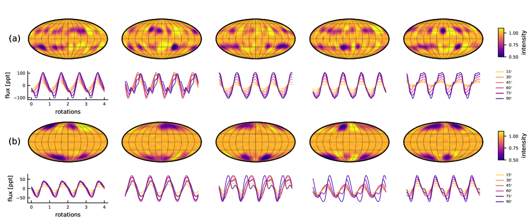
Figure 1: Five random samples from our GP (columns) conditioned on two different hyperparameter vectors $\boldsymbol{\theta}_{\bullet}$ (rows). The samples are shown on the surface of the star in a Mollweide projection alongside the corresponding light curves viewed at several different inclinations. (a) Samples from a GP describing a star with small mid-latitude spots. (b) Samples from a GP describing a star with larger high-latitude spots.

Statement of need

Mapping the surfaces of stars using time series measurements is a fundamental problem in modern time-domain stellar astrophysics. This inverse problem is ill-posed and computationally intractable, but in the associated AAS Journals publication submitted in parallel to this paper (Luger, Foreman-Mackey, & Hedges, 2021), we derive an interpretable effective Gaussian Process (GP) model for this problem that enables robust probabilistic characterization of stellar surfaces using photometric time series observations. Our model builds on previous work by Perger et al. (2020) on semi-interpretable Gaussian processes for stellar timeseries data and by Morris (2020) on approximate inference for large ensembles of stellar light curves. Implementation of our model requires the efficient evaluation of a set of special functions and recursion relations that are not readily available in existing probabilistic programming frameworks. The starry_process package provides the necessary elements to perform this analysis with existing and forthcoming astronomical datasets.

Implementation

We implement our interpretable GP in the user-friendly Python package starry_process, which can be installed via pip or from source on https://github.com/rodluger/starry_processhttps://doi.orgGitHub. The code is thoroughly https://github.com/rodluger/starry_process/tree/master/testshttps://doi.orgunit-tested and https://starry_process.readthedocs.iohttps://doi.orgwell documented, with https://starry-process.readthedocs.io/en/latest/exampleshttps://doi.orgexamples on how to use the GP in custom inference problems. As discussed in the associated AAS Journals publication (Luger, Foreman-Mackey, & Hedges, 2021), users can choose, among other options, whether or not to marginalize over the stellar inclination and whether or not to model a normalized process. Users can also choose the spherical harmonic degree of the expansion, although it is recommended to use $l_{\mathrm{max}}=15$ (see below). Users may compute the mean vector and covariance matrix in either the spherical harmonic basis or the flux basis, or they may sample from it or use it to compute marginal likelihoods. Arbitrary order limb darkening is implemented following Agol et al. (2020).

The code was designed to maximize the speed and numerical stability of the computation. Although the computation of the GP covariance involves many layers of nested sums over spherical harmonic coefficients, these may be expressed as high-dimensional tensor products, which can be evaluated efficiently on modern hardware. Many of the expressions can also be either pre-computed or computed recursively. To maximize the speed of the algorithm, the code is implemented in hybrid C++/Python using the just-in-time compilation capability of the Theano package (Theano Development Team, 2016). Since all equations derived here have closed form expressions, these can be autodifferentiated in a straightforward and numerically stable manner, enabling the computation of backpropagated gradients within Theano. As such, starry_process is designed to work out-of-the box with Theano-based inference tools such as PyMC3 for NUTS/HMC or ADVI sampling (Salvatier et al., 2016).

Figure 2 shows the computational scaling of the Python implementation of the algorithm for the case where we condition the GP on a specific value of the inclination (blue) and the case where we marginalize over inclination (orange). Both curves show the time in seconds to compute the likelihood (averaged over many trials to obtain a robust estimate) as a function of the number of points $K$ in a single light curve. For $K\lesssim 100$, the computation time is constant at $10-30$ ms for both algorithms. This is the approximate time (on a typical modern laptop) taken to compute the GP covariance matrix given a set of hyperparameters $\boldsymbol{\theta}_{\bullet}$. For larger values of $K$, the cost approaches a scaling of $K^{2.6}$, which is dominated by the factorization of the covariance matrix and the solve operation to compute the likelihood. The likelihood marginalized over inclination is only slightly slower to compute, thanks to the tricks discussed in Luger, Foreman-Mackey, & Hedges (2021).

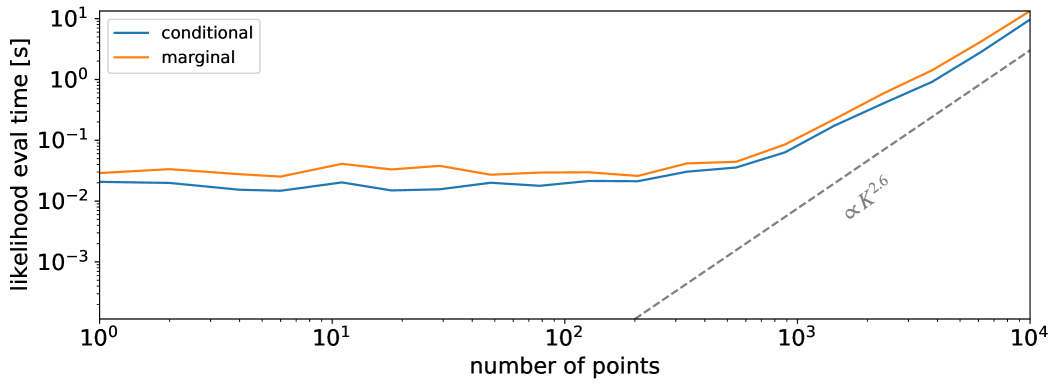
Figure 2: Evaluation time in seconds for a single log-likelihood computation as a function of the number of points $K$ in each light curve when conditioning on a value of the inclination (blue) and when marginalizing over the inclination (orange). At $l_{\mathrm{max}}=15$, computation of the covariance matrix of the GP takes about 20ms on a typical laptop. The dashed line shows the asymptotic scaling of the algorithm, which is due to the Cholesky factorization and solve operations.

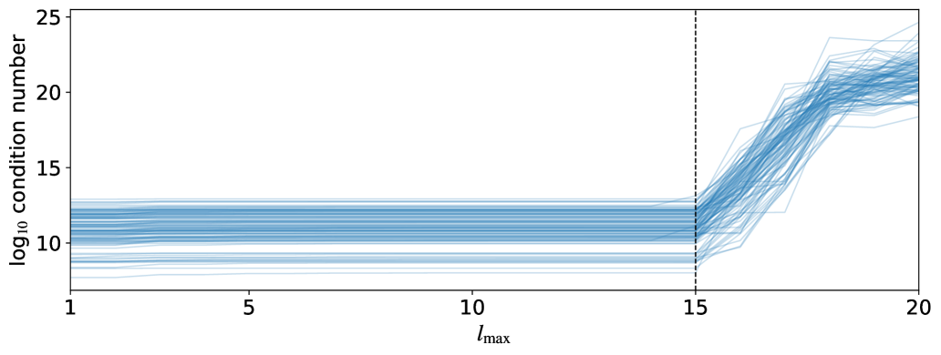
Figure 3: Log of the condition number of the covariance in the spherical harmonic basis as a function of the spherical harmonic degree of the expansion, $l_{\mathrm{max}}$. Different lines correspond to different values of $\boldsymbol{\theta}_{\bullet}$ drawn from a uniform prior (see text for details). In the majority of the cases, the matrix becomes ill-conditioned above $l_{\mathrm{max}}=15$.

Many modern GP packages (e.g., Ambikasaran et al., 2015; Foreman-Mackey et al., 2017) have significantly better asymptotic scalings, but these are usually due to specific structure imposed on the kernel functions, such as the assumption of stationarity. Our kernel structure is determined by the physics (or perhaps more accurately, the geometry) of stellar surfaces, and its nonstationarity is a consequence of the normalization step in relative photometry (Luger, Foreman-Mackey, Hedges, & Hogg, 2021). Moreover, and unlike the typical kernels used for GP regression, our kernel is a nontrivial function of the hyperparameters $\boldsymbol{\theta}_{\bullet}$, so its computation is necessarily more expensive. Nevertheless, the fact that our GP may be used for likelihood evaluation in a small fraction of a second for typical datasets ($K\sim 1{,000}$) makes it extremely useful for inference.

Our algorithm is also numerically stable over nearly all of the prior volume up to $l_{\mathrm{max}}=15$. Figure 3 shows the log of the condition number of the covariance matrix in the spherical harmonic basis as a function of the spherical harmonic degree of the expansion for 100 draws from a uniform prior over the domain of the hyperparameters. The condition number is nearly constant up to $l_{\mathrm{max}}=15$ in almost all cases; above this value, the algorithm suddenly becomes unstable and the covariance is ill-conditioned. The instability occurs within the computation of the latitude and longitude moment integrals and is likely due to the large number of operations involving linear combinations of hypergeometric and gamma functions. While it may be possible to achieve stability at higher values of $l_{\mathrm{max}}$ via careful reparametrization of some of those equations, we find that $l_{\mathrm{max}}=15$ is high enough for most practical purposes.

References

Agol, E., Luger, R., & Foreman-Mackey, D. (2020). Analytic Planetary Transit Light Curves and Derivatives for Stars with Polynomial Limb Darkening. 159(3), 123. https://doi.org/10.3847/1538-3881/ab4fee

Ambikasaran, S., Foreman-Mackey, D., Greengard, L., Hogg, D. W., & O’Neil, M. (2015). Fast Direct Methods for Gaussian Processes. IEEE Transactions on Pattern Analysis and Machine Intelligence, 38, 252. https://doi.org/10.1109/TPAMI.2015.2448083

Foreman-Mackey, D., Agol, E., Ambikasaran, S., & Angus, R. (2017). Fast and Scalable Gaussian Process Modeling with Applications to Astronomical Time Series. 154(6), 220. https://doi.org/10.3847/1538-3881/aa9332

Luger, R., Foreman-Mackey, D., & Hedges, C. (2021). Mapping stellar surfaces II: An interpretable Gaussian process model for light curves. arXiv e-Prints, arXiv:2102.01697. http://arxiv.org/abs/2102.01697

Luger, R., Foreman-Mackey, D., Hedges, C., & Hogg, D. W. (2021). Mapping stellar surfaces I: Degeneracies in the rotational light curve problem. arXiv e-Prints, arXiv:2102.00007. http://arxiv.org/abs/2102.00007

Morris, B. (2020). fleck: Fast approximate light curves for starspot rotational modulation. The Journal of Open Source Software, 5(47), 2103. https://doi.org/10.21105/joss.02103

Perger, M., Anglada-Escudé, G., Ribas, I., Rosich, A., Herrero, E., & Morales, J. C. (2020). Auto-correlation functions of astrophysical processes, and their relation to Gaussian processes; Application to radial velocities of different starspot configurations. arXiv e-Prints, arXiv:2012.01862. http://arxiv.org/abs/2012.01862

Salvatier, J., Wiecki, T. V., & Fonnesbeck, C. (2016). Probabilistic programming in Python using PyMC3. PeerJ Computer Science, 2, e55.

Theano Development Team. (2016). Theano: A Python framework for fast computation of mathematical expressions. arXiv e-Prints, abs/1605.02688. http://arxiv.org/abs/1605.02688