Measuring solar neutrinos over Gigayear timescales with Paleo Detectors

Abstract

Measuring the solar neutrino flux over gigayear timescales could provide a new window to inform the Solar Standard Model as well as studies of the Earth’s long-term climate. We demonstrate the feasibility of measuring the time-evolution of the ⁸B solar neutrino flux over gigayear timescales using paleo detectors, naturally occurring minerals which record neutrino-induced recoil tracks over geological times. We explore suitable minerals and identify track lengths of 15–30 nm to be a practical window to detect the ⁸B solar neutrino flux. A collection of ultra-radiopure minerals of different ages, each some 0.1 kg by mass, can be used to probe the rise of the ⁸B solar neutrino flux over the recent gigayear of the Sun’s evolution. We also show that models of the solar abundance problem can be distinguished based on the time-integrated tracks induced by the ⁸B solar neutrino flux.

I Introduction

The concept of “Solar Activity” is used by the scientific community to study the fact that the Sun is not a static quiet object and, in contrast to what was thought in ancient times, evolves Usoskin (2008). Studying and understanding solar activity not only benefits science itself, but affects directly our environment as living beings and has broad implications: strong solar activity affects directly our communications and travel systems and of course, our planet’s climate Bond et al. (2001); Beer et al. (2000); Ribas et al. (2005).

Fundamental to the study of the evolution of the Sun is the Solar Standard Model (SSM), a theoretical tool to investigate the solar interior. First attempts to build a solar model to understand and predict more accurately its core central temperature and to estimate the rates of solar neutrinos started in the mid 20th century, and culminated in the SSM by Bahcall et al. Bahcall et al. (1968). Over the decades, the SSM has been developed and stringently tested with a variety of measurements, not only neutrinos but also helioseismology (for recent reviews, see, e.g., Haxton et al. (2013a)).

Initial measurements of the solar neutrinos resulted in less neutrinos than predicted by the SSM, known as the “solar neutrino problem.” Many solutions were developed based on producing a cooler solar core, but the phenomenon of neutrino oscillations Pontecorvo (1968) proved the correct solution with the discovery of the matter-induced Mikheyev-Smirnov-Wolfenstein mechanism Mikheyev and Smirnov (1985); Wolfenstein (1979, 1978); Mikheev and Smirnov (1986) and direct measurement of all neutrino flavours of solar neutrinos by the Sudbury Neutrino Observatory (SNO) experiment Ahmad et al. (2002); McDonald (2016). Presently, much of the solar neutrino flux has been experimentally verified (see, e.g., Haxton et al. (2013a); Wurm (2017)). In addition, helioseismic observations probe important properties of the solar interior, such as the sound speed profile, depth of the convective envelope, and surface helium abundance, to percent or better precision (e.g., Degl’Innocenti et al. (1997); Gough et al. (1996)). As a result, the solar structure is now very well constrained. By now, solar neutrinos and helioseismology provide a clear view of the present energy generation rate of the Sun. By contrast, photons reveal the power generation roughly $10^{4}$–$10^{5}$ years ago, corresponding to the energy transport timescale within the solar interior Mitalas and Sills (1992). Within measurement uncertainties, the neutrino and photon observations match, revealing the stability of the solar activity on $\sim 10^{5}$ year scales.

However, recent measurements of the solar elemental abundances (metallicity) by Asplund et al. 2009 (hereafter AGSS) Asplund et al. (2009) have caused a new conflict within the SSM. The new photospheric measurements indicate that the solar metallicity is lower than previously estimated by Grevesse & Sauval 1998 (hereafter GS) Grevesse and Sauval (1998). The SSM is sensitive to transitions in metals (used to refer to anything above helium), which are an important contributor to opacity. Lower metallicity is associated with a cooler solar core, and in this way, affects the solar interior. Solar models using the new metallicity are no longer able to reproduce helioseismic results, causing the so-called “solar abundance problem” Haxton et al. (2013a); Serenelli et al. (2009). Extended SSMs, where some of the assumptions of the SSM are relaxed, have been explored as potential solutions, e.g., early accretion causing chemical inhomogeneities Serenelli et al. (2011). While the debate continues, a pragmatic approach has been to use two sets of SSMs with different metallicities. Neutrinos are one way to observationally test the solar abundance problem through their dependence on the metallicity of the stellar interior. A lower metallicity causes a lower core temperature which in turn has a strong impact on neutrino fluxes, in particular those involving nuclei in their production chain, e.g., ⁸B, CNO neutrinos.

Detecting weakly-interacting particles like solar neutrinos requires immense volumes to instrument enough target numbers to have an appreciable number of neutrino interactions. The same difficulties faced by neutrino measurements are encountered in direct searches for dark matter, where experiments seek to observe the scattering of target nuclei by an incoming dark matter particle. Recently, it has been proposed that rock crystals deep in the Earth could act as a new method to detect dark matter Drukier et al. (2019); Edwards et al. (2019a, b); Baum et al. (2020a). Called “paleo detectors”, the idea is that dark matter interactions will leave permanent structure or chemical changes (tracks) caused by the recoiling nuclei within the rocks. By strategically collecting samples from geologically quiet areas, the tracks can survive geological periods and measured in the lab through small angle X-ray scattering. And by sampling from deep underground, backgrounds caused by cosmic-ray interactions in the Earth atmosphere can be mitigated. An unavoidable background comes from radioactivity of the Earth, but this can be rejected based on their rich track signatures. Furthermore, paleo detectors have competitive exposures compared to terrestrial experiments. Exposure is the product of the target mass and duration in time. In the case of paleo detectors, $\sim 1$ Gyr old samples are possible, so even a small mass of $10\,\text{mg}$ would be competitive with a terrestrial experiment of $10^{3}\,\text{kg}$ running for 10 years: both have exposures $\varepsilon=0.01\,\text{kg Myr}$.

In this paper, we consider the detectability of solar neutrinos using paleo detectors. The energies of solar neutrinos are about $\sim 1\,\text{MeV}$, which translate to $\sim\text{keV}$ of recoil energy. This is comparable to the recoil energies $E_{R}=0.1-100\,\text{keV}$ caused by dark matter, meaning solar neutrinos should also give rise to damage tracks. Importantly, paleo detectors not only open a new way to search for solar neutrinos, they allow us to probe the Sun in the past on Gyr time scales, something that is not possible with terrestrial detectors. Recently, paleo detectors have been considered also as detectors of supernova neutrinos Baum et al. (2020b) and atmospheric neutrinos Jordan et al. (2020) over similar geological times. To investigate the study of the SSM with paleo detectors, we compute two SSMs that differ in their metallicity. We focus on the ⁸B neutrino flux, which shows strong dependence on the solar interior temperature and metallicity models. The ⁸B neutrinos are also among the highest in energy, making them easier to detect compared to other higher-flux but lower-energy solar neutrino components.

This paper is organized as follows. In Section II, we go through our computation of the history of the solar neutrino flux with different metallicities which give us the time dependency of the flux. Section III goes through the track formation process, mineral choice, and a basic mathematical framework to compute the estimated number of tracks for each SSM. In Section IV, we use the time-dependent track estimates to check the behaviour or variation in time for our two metallicity models. Finally in Section V we discuss our results and conclude.

II Solar Neutrino & Metallicity Models

Solar neutrinos arise from multiple reactions within the solar core. We focus on the ⁸B neutrinos due to their higher neutrino energies which facilitates detection, and also for their strong dependence on the solar core temperature, approximately $\propto T^{24}$ (by contrast, the dominant $pp$ chain has a $\propto T^{4}$ dependence) Bahcall and Ulmer (1996). Since most of the ⁸B flux is emitted from the interior 5–10% of the solar radius, the ⁸B neutrinos provide a probe of the solar interior. It is sensitive to the interior metal abundance, due to the metallicity’s influence on the electromagnetic opacity and hence temperature gradient inside the Sun.

We model the Sun using the MESA code version r12115 Paxton et al. (2011, 2013, 2015, 2018, 2019), closely following the procedure outlined in Farag et al. 2020 Farag et al. (2020). We adopt their solar models calibrated to reproduce the present day neutrino fluxes, with final age $t_{\odot}=4.568$ Gyr Bouvier and Wadhwa (2010), radius $R_{\odot}=6.9566\times 10^{10}$ cm Prša et al. (2016), photon luminosity $L_{\gamma}=3.828\times 10^{33}$ erg/s Prša et al. (2016), and surface metallicity $Z/X$. These are obtained by using the built-in MESA simplex module to vary iteratively the mixing-length parameter and the initial hydrogen, helium, and metal compositions, including the effects of element diffusion Paxton et al. (2018). The helioseimic signals of these models have been confirmed to be similar to others in the literature Villante et al. (2014). We refer the reader to Ref. Farag et al. (2020) for further details of the calculations.

We compute two SSMs made to match two different abundance of heavy metals at the surface of the Sun: $Z/X=0.0229$ for GS Grevesse and Sauval (1998) and $Z/X=0.0181$ for AGSS Asplund et al. (2009). We use the built-in MESA reaction network add_pp_extras to model the reactions emitting neutrinos, including $pp$, $pep$, ⁷Be, and ⁸B. For the CNO chain, we use the add_cno_extras and add_hot_cno and compute the neutrinos from ¹³N, ¹⁵O, and ¹⁷F. Our obtained neutrino fluxes for the two metallicity models, compared to experimentally measured values, are listed in Table 1. Our predicted fluxes are similar to those in the literature Haxton et al. (2013b); Villante et al. (2014); Farag et al. (2020). In Figure 1, we show the time evolution of these neutrino fluxes, as a function of years in the past. We show results only for the GS metallicity model, as the AGSS is very similar on these scales.

Channel	GS	AGSS	Measurement
$\Phi_{\rm pp}$	5.98	6.01	$6.05(1^{+0.003}_{-0.011})$
$\Phi_{{}^{7}{\rm Be}}$	4.95	4.71	$4.82(1^{+0.05}_{-0.04})$
$\Phi_{{}^{8}{\rm B}}$	5.09	4.62	$5.00(1\pm 0.03)$
$\Phi_{\rm CNO}$	5.12	3.92	$7.0(1^{+0.43}_{-0.29})$

Table 1: Observed solar neutrino fluxes at Earth, predicted by MESA and measured, in units of [cm^-2 s^-1], with the following scales: $10^{10}$ ($pp$), $10^{9}$ (7Be), $10^{6}$ (B), and $10^{8}$ (CNO). Measurements are from Ref. Bellini et al. (2011) as summarized in Refs. Haxton et al. (2013b); Villante et al. (2014); Farag et al. (2020), and updated by Borexino’s measurement of the CNO flux Agostini et al. (2020).

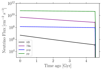
Figure 1: Neutrino flux variation over time, for different components of the solar neutrino flux, for the GS metallicity model.

III Rates per track length spectrum

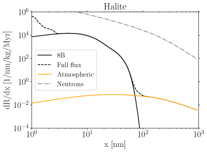
Figure 2: Track length spectra for sinjarite (left panel) and halite (right panel). Shown are the tracks induced by neutrinos and neutrons, as labeled. The tracks caused by the ⁸B flux and atmospheric neutrinos are shown separately for clarify. The central peak above tens of nm is induced by the ⁸B flux, while above around $200$ nm the tracks are induced by the atmospheric neutrino flux, while below 2–3 nm the tracks arise from the contributions of multiple solar neutrino components with lower energies than ⁸B.

When an incoming particle collides with a target rock crystal, it is slowed down and eventually stopped, during which time its energy is deposited in the form of tracks, that is, permanent damages made in the rock. The shape and length of these tracks allow one to reconstruct the mass, energy and even direction of the incoming particle ILIA and DURRANI (2003). The formation of tracks is dependent on the response of the material, which in turn depend on the chemistry of the material. In this section, we first discuss our material selection, and we review the computation of tracks formed by solar neutrinos and backgrounds. For more details, we refer the reader to, e.g., Refs. Baum et al. (2020a); Edwards et al. (2019b, a); Drukier et al. (2019).

In analogy to direct dark matter detection experiments, low radioactive contamination is a crucial part of material selection. The major consideration is the material’s Uranium concentration. There are two processes by which ²³⁸U could leave tracks: $\alpha$ decay and spontaneous fission. Spontaneous fission of ²³⁸U nuclei gives rise to approximately two $\sim 1\,\text{MeV}$ fast neutrons. Neutrons are also produced in ($\alpha$, n) reactions, where nuclei absorb an incident $\alpha$ particle and emit fast neutrons. These neutrons act similarly to solar neutrinos in their formation of tracks in the material. Cosmic rays can also cause potential background track events. However, they can be mitigated by using paleo detector material from deep underground. The primary concern will be neutrons arising from cosmic-ray muons interacting with nuclei near the target material. By a depth of $\sim 6$ km however, the estimated neutron flux is $\sim 10\,{\rm cm^{-2}\,Gyr^{-1}}$ Mei and Hime (2006). As we discuss below, we consider targets of 0.1 kg in mass corresponding to cross-sectional areas of $\sim 10\,{\rm cm^{2}}$, implying background from cosmic-ray induced neutrons will be negligible. For a detailed description of the neutron backgrounds, see Ref. Drukier et al. (2019).

We follow Ref. Edwards et al. (2019a) and start with four minerals (olivine, nchwaningite, halite, and sinjarite), chosen because of their low levels of natural radioactive contamination. Olivine and Nchwaningite are examples of ultra basic rocks (UBR), which stem from the Earth’s mantle Bowes (1990) and are more radiopure than the average Earth crust. We follow Ref. Edwards et al. (2019a) and adopt a Uranium concentration of $0.1$ parts per billion for UBRs. Halite and Sinjarite are marine evaporites (ME) formed after extreme evaporation of seawater Dean (2013) and are even more radiopure. We follow Ref. Edwards et al. (2019a) and adopt Uranium concentrations of $0.01$ parts per billion for MEs.

Furthermore, the difference in the chemical composition of these minerals also has two important implications: first, they impact the rate of neutron background recorded, and second, they impact the response, i.e., the length distribution of tracks given a neutrino spectrum. As we will show, hydrogen is a good moderator of fast neutrons, making minerals containing hydrogen attractive as solar neutrino detectors. Two of the minerals we consider contain hydrogen: nchwaningite (${\rm Mn}_{2}^{2+}{\rm SiO}_{3}({\rm OH})_{2}\cdot({\rm H}_{2}{\rm O})$), a type of UBR, and sinjarite (${\rm CaCl}_{2}\cdot 2({\rm H}_{2}{\rm O})$), a type of ME.

We base our estimates of track formation on the calculations of Ref. Edwards et al. (2019b). Here, we review the main ingredients and describe how we adapt it to compute tracks from a time-dependent solar neutrino flux. The ionization track length for a recoiling nucleus $T$ with initial recoil energy $E_{R}$ is

$$x_{T}(E_{R})=\int_{0}^{E_{R}}dE\left(\frac{dE}{dx_{T}}(E)\right)^{-1},$$ (1)

where $dE/dx_{T}$ is the stopping power for a recoiling nucleus $T$ incident on an amorphous target. If the target material has different components, the stopping power is the sum of the different contributions $V$

$$\frac{dE}{dx_{T}}=\sum_{V}\left(\frac{dE}{dx}\right)_{VT}.$$ (2)

The stopping power is obtained from the SRIM code Ziegler et al. (2010), which differs at the $10\%$ level from analytical calculations Baum et al. (2020a). Track formation from ions with charge $Z\gtrsim 10$ and recoil energies larger than a few keV are well studied, but the situation is less clear for lighter ions Drukier et al. (2019). Thus, we do not include hydrogen as a potential source of tracks, and we show in the appendix results when hydrogen induced tracks are included.

In the search for solar neutrinos, fast neutrons pose a significant background. We model the neutron induced recoil spectra following Ref. Edwards et al. (2019a), which in turn is based on the sources-4A code Wilson et al. (2005), for the spontaneous fission and $(\alpha,n)$ contributions to the background. The code uses the parameters of 43 actinides and their half lives and spontaneous fission branches, to obtain the spontaneous fission spectra of neutrons. The spontaneous fission neutron spectra are approximated by a Watt fission spectrum. For the $(\alpha,n)$ channel, an isotropic neutron angular distribution in the centre-of-mass system is assumed. The spectra can be computed using this set up, see, e.g., Ref. Madland et al. (1999). The average number of neutrons must be known, which is supplied by the assumed Uranium concentration. In Figure 2, we show the neutron-induced track length spectra for sinjarite and halite with assumed Uranium concentrations of 0.01 parts per billion using dot-dashed grey lines.

Next, we compute the track length spectra induced by neutrinos. We consider the differential solar neutrino flux to study the tracks left during different time epochs of the Sun’s history. The neutrino induced differential recoil spectrum per unit mass of target nuclei $T$ is given by

$$\left(\frac{dR}{dE_{R}}\right)_{T}=\frac{1}{m_{T}}\int_{E_{\nu}^{min}}dE_{\nu}\int_{\Delta t}dt\frac{d\sigma}{dE_{R}}\frac{d^{2}\Phi_{\nu}}{dE_{\nu}dt},$$ (3)

where $E_{\nu}^{min}=\sqrt{m_{T}E_{R}/2}$ is the minimum energy required in order to produce a nuclear recoil with energy $E_{R}$ and $d^{2}\Phi/dEdt$ is the differential solar neutrino flux. We adopt the time-dependent ⁸B flux as described in Section II, keeping the spectral shape of neutrinos fixed. Contrary to the flux which depends very strongly on the temperature, the spectral corrections due to thermal broadening are minimal. In practice, the code of Ref. Edwards et al. (2019b) assumes a constant solar neutrino flux, so we re-scale the track predictions by the ratio of integrated flux of neutrinos over time bins of interest. The differential cross section for coherent neutrino-nucleus scattering is

$$\frac{d\sigma}{dE_{R}}(E_{R},E_{\nu})=\frac{G_{F}^{2}}{4\pi}\,Q_{W}^{2}m_{T}\left(1-\frac{m_{T}E_{R}}{2E_{\nu}^{2}}\right)\,F^{2}(E_{R})$$ (4)

where $G_{F}$ is the Fermi coupling constant, $F(E_{R})$ is the nuclear form factor, $Q_{W}\equiv\left(A_{T}-Z_{T}\right)-\left(1-4\sin{\theta_{W}}^{2}\right)Z_{T}$ and $\theta_{W}$ is the weak mixing angle. Finally, the track length spectra is obtained by summing over the target nuclei in the mineral,

$$\frac{dR}{dx}=\sum_{T}\xi_{T}\frac{dE_{R}}{dx_{T}}\left(\frac{dR}{dE_{R}}\right)_{T},$$ (5)

where $\xi_{T}$ is the mass fraction of each constituent nuclei $T$.

There are other sources of neutrinos that could leave tracks over our track lengths of interest. One example is atmospheric neutrinos. We compute this using the Honda atmospheric neutrino model Honda et al. (2011). Another example is the diffuse supernova neutrino background (DSNB) O’Hare (2016), which we do not explicitly consider due to their much smaller relative contributions Edwards et al. (2019b). In fact, the neutrinos from supernovae in the Milky Way galaxy yields a higher flux over geological times than the DSNB Baum et al. (2020b), yet even that is lower than the ⁸B neutrino flux by orders of magnitude in the 1–10 MeV energy range.

In Figure 2, we show the neutrino-induced track spectra, highlighting the different neutrino components, for sinjarite (left panel) and halite (right panel). The longest tracks, left by the highest energy neutrinos, are unsurprisingly induced by atmospheric neutrinos, shown by the solid orange curves. For halite, the neutrino induced tracks are however overwhelmed by the much more numerous neutron induced tracks. On the other hand, for sinjarite the neutrino induced tracks exceed the neutron background tracks below track lengths of $\sim 30$ nm. Below 10 nm, the tracks are dominated by a mixture of multiple solar neutrino components, including ⁷Be, pep, and CNO. Therefore, at intermediate track lengths between 10–30 nm, there is a window where the ⁸B neutrino flux is the dominant source, exceeding also the neutron-induced background.

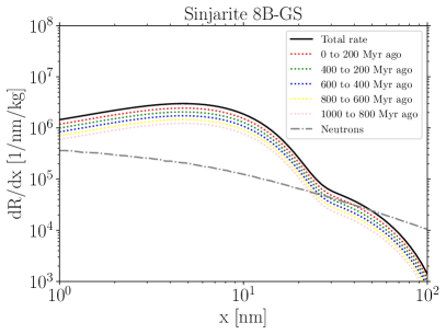
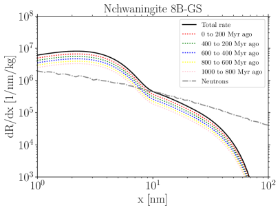
Figure 3: Same as Fig. 2 but showing the tracks induced by the ⁸B flux over time bins of 200 Myr widths. The neutron background from radioactive processes can be seen in gray dashed line and remains the same for every 200 Myr bin.

The tracks spectrum induced by solar neutrinos in sinjarite show a kink at around 30 nm. This is not due to a feature in the neutrino spectrum, but rather, is associated with the transition in tracks left by different nuclei of the sinjarite crystal (${\rm CaCl}_{2}\cdot 2({\rm H}_{2}{\rm O})$). Below track lengths of $\sim 30$ nm, the contribution is dominated by recoils of Cl and Ca, whereas above $\sim 30$ nm, O recoils dominate. This is not because of the number of tracks it would create, but because of their recoil kinematics and the resulting tracks lengths they reach.

The kink is not as apparent in halite (see right panel of Figure 2) and olivine which have a different chemical composition and the transition between the different nuclei of each mineral component is much softer.

In Figure 3, we show the track spectra in 200 Myr time bins, for sinjarite (left panel) and nchwaningite (right panel). These are two materials with a large detection window for ⁸B neutrino induced tracks. The composition of these minerals is what makes them good candidates for our study, in contrast to Olivine and Halite; see also Fig. 1 of Ref. Edwards et al. (2019b).

IV Results

IV.1 Time variation of number of events

We start our analysis with the detectability of the time-evolution of tracks induced by the time-dependent solar neutrino flux. This requires measuring the total number of tracks in multiple mineral samples of different ages. We consider paleo detectors with ages up to 1 Gyr with 200 Myr age accuracy. It is expected tracks would be preserved for around 1 Gyr, but beyond this time scale, they could fade due to annealing of the rocks under the high temperatures encountered deep underground Drukier et al. (2019). Our choice of 200 Myr time bins is motivated by the precision of techniques to date rock samples. The most relevant method for dating Gyr-aged rocks is fission track dating, which is expected to be reliable at the level of $\sim 10$% Gallagher et al. (1998).

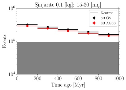
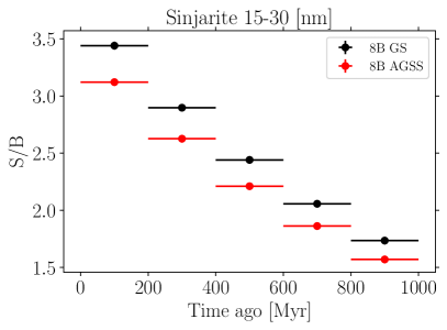
Figure 4: Left: Number of events per 200 Myr time bins, for 0.1 Kg of Sinjarite. Events are summed over track lengths of 15 to 30 nm. The black dots represent the GS (reference) SSM and red represents AGSS SSM. The shaded region is where the neutron backgrounds will dominate the events. Right: signal-to-background ratio, separately for the GS and AGSS models. The time binning is the same as on the left panel.

We consider different exposure scenarios following Ref. Edwards et al. (2019a). Our default assumption is a mineral of mass of 0.1 kg and a minimal track length resolution of 15 nm. This corresponds to the assumed resolution and mass of the “high exposure” case of Ref. Edwards et al. (2019a). Note that this implies exposures of $\varepsilon\sim 20\,\text{Kg Myr}$ for each of our 200 Myr time bins.

The tracks which have persisted over time could be read out with helium ion beam microscope, with spatial resolution of $\sim$ nm and able to image up to depths of $O(100)$ nm Drukier et al. (2019). Small angle X-ray scattering can achieve $\sim 15$ nm three dimensional spatial resolution, which is our adopted minimum length sensitivity, and it can measure up to $O(100)$ g of material, also our choice of sample mass. The peak of the ⁸B track length spectra actually lies at lower lengths ($\sim 7$ nm for sinjarite), which would provide a more favorable signal over background ratio than our 15 nm minimum track length. However, measuring tracks as small as $7\,\text{nm}$ will need technology development and we conservatively assume the more established 15 nm resolution. In the Appendix, we show results for a 10 nm resolution case.

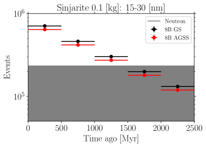
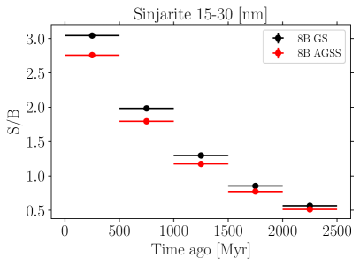
Figure 5: The same as Fig. 4, but extending out to 2.5 Gyr and with wider 500 Myr time bins.

To maximize the signal to noise, we consider a maximum track length of 30 nm. As can be seen in the left panel of Figure 3, this helps to mitigate the neutron background which starts exceeding the ⁸B neutrino events above 30 nm. In the case of nchwaningite (Figure 3 right panel), the peak is more pronounced around track length of 2 nm, and by 15 nm the ratio of signal over background is already disfavoured. This difference is caused by the the different nuclear compositions which in turn determine the recoil response to the same ⁸B neutrino spectrum. Thus, we find a strong preference for sinjarite over nchwaningite, even though they both share the benefit of containing hydrogen in their molecular structures. We note that in these estimates we assume hydrogen do not efficiently leave tracks. In the appendix, we discuss how the results numerically change if they are included.

Our main results, for two metallicity models and different time windows, are shown in Figure 4 where we show the total number of events per time bin (left panel) and the computed signal-to-noise per time bin (right panel), both for sinjarite. We see that in every time bin, the signal over background ratio is above 1, reaching $\sim 3.5$ for the most recent past.

Going beyond $\sim 1$ Gyr in the past poses additional difficulties. In addition to the effects of heat annealing, the signal become overwhelmed by backgrounds. In Figure 5 we show the reach up to 2.5 Gyr in 500 Myr time bins. We see that beyond 1–1.5 Gyr the solar neutrino induced tracks fall below the neutrino signal, and measuring the solar neutrino tracks become difficult. However, the situation improves if a higher resolution can be achieved. In the Appendix we consider the case of a track resolution of 10 nm. An improvement with respect to our 15–30 nm case is expected from Figure 3, but it has a qualitatively important impact for measuring the solar activity beyond the 1 Gyr age, provided paleo detectors of those ages can be found.

IV.2 Sensitivity to metallicity model

For our 200 Myr time bin width result (Figure 4), the difference between the GS and AGSS metallicity models is $\sim 10^{4}$ tracks per time bin, i.e., approximately $\sim 10$% of the track counts. As can be seen in the panels, the difference between GS and AGSS is more or less time independent. Thus, we can sum over the entire 1 Gyr range for maximum statistics. The total number of tracks is $\sim 1.17\times 10^{6}$ and $\sim 1.06\times 10^{6}$, for GS and AGSS, respectively. If we assume only Poisson errors, then $\sigma\sim 10^{3}$, and a difference of 10% due to the metallicity models would be easy to measure.

In reality, the measurement will be dominated by systematic effects. So far, we have assumed the major source of background arising from neutron tracks is perfectly known. The uncertainty of this background is related to the initial concentration of radioactive material present in the crystal. The initial radioactivity can then be estimated by the number of whole decays chains identified through long tracks. Thus, the normalization of the neutron background is likely to be estimated to high precision.

Nevertheless, to study the potential impacts of any uncertainty on the mineral’s radioactivity, we assume two situations: a $1\%$ systematic uncertainty in the neutron background, as well as up to $10\%$ uncertainty. In both cases, it would be possible to distinguish the two metallicity models. For example, for the 10% case, the total number of tracks over the 1 Gyr window in the GS and AGSS metallicity models is $(1.63\pm 0.05)\times 10^{6}$ and $(1.52\pm 0.05)\times 10^{6}$ tracks, respectively. Here, the numbers include the number of tracks caused by fast neutron ($\sim 5\times 10^{5}$) and the error bars represent a $\pm 10$% uncertainty of the neutron induced tracks. Even with this generous uncertainty, it would be possible to gain insight into the metallicity models based on total number of tracks.

V Conclusions

We have considered SSMs with two metallicities (GS and AGSS) to study the detectability of the boron-8 (⁸B) solar neutrino flux over gigayear timescales using paleo detectors. Our default setup is a paleo detector composed of a collection of 0.1 kg of sinjarite crystals of different ages, up to 1 Gyr old and aged with 200 Myr resolution, but we also consider an older sample reaching 2.5 Gyr with 500 Myr age-dating resolution. We identified track lengths of 15–30 nm to be the most suitable for detecting the ⁸B neutrino flux with established technologies. We found that up to 1–1.5 Gyr, the ⁸B signal to background ratio is favourable for measuring the time-evolution of the ⁸B neutrino flux and for distinguishing the two metallicity models.

The main background to solar neutrinos is caused by fast neutrons, originating from radioactive sources within the minerals. The normalization of this background solely depends on the original concentration of radioactive materials. We follow Ref. Drukier et al. (2019) and adopt a Uranium concentration of 0.01 parts per billion for sinjarite. Since the neutron background rate scales with this concentration, the detectability of the ⁸B neutrino flux with sinjarite requires the concentration to be not more than a few times 0.01 parts per billion. In principle this concentration can be measured, e.g., using the number of full ²³⁸U decay chains in the target mineral as probed by longer tracks, and therefore constrained accurately. We follow Ref. Drukier et al. (2019) and assume a normalization uncertainty of 1%. Nevertheless, we also check up to $10\%$ uncertainty and we find that the two metallicity solar models can be differentiated even with the larger background uncertainty.

Among the paleo detector materials discussed in the literature (e.g., Edwards et al. (2019a, b)), we identify sinjarite as uniquely optimal for solar neutrino studies. Its hydrogen component helps to reduced neutron backgrounds by slowing them and reducing the numbers of tracks related to this source. Nchwaningite is another material studied in the literature Edwards et al. (2019b) and like sinjarite contains a hydrogen component. It is a good candidate with good signal to background ratios for shorter tracks. This mineral would be competitive in the future when technology and theory will allow measurements and interpretations of $<10$ nm tracks.

To conclude, paleo detectors represent a novel and intriguing opportunity to uniquely probe solar neutrinos on gigayear timescales. This could open a new window to inform the Solar Standard Model, as well as measure the past solar activity and guide inputs for solar system planetary climates.

Appendix A Other Results

Here, we explore additional cases. First, we consider a track length sensitivity as short as 10 nm. This is a more optimistic scenario compared to our default 15 nm, and will require R&D for better measuring instruments. Exploring shorter track lengths implies, in terms of WIMP Dark Matter masses for example, going to smaller masses. Similarly, for solar neutrino search it opens new track length regimes to perform higher signal to background searches. We show the results in Figure 6, which is to be contrasted with Figure 5. Here, we also take 500 Myr time bins and 0.1 Kg of material. The gains due to the improved sensitivity become noticeable over these few Gyr timescales. For example, up to 2 Gyr the signal over background ratio is favourable, which was not possible when the track length sensitivity is 15 nm.

Figure 6: Same as Fig. 5, but summed over a wider track lengths of 10–30 nm.

Next, we also check the time evolution of the same mineral, sinjarite, but now considering also tracks formed by hydrogen recoils. This channel is neglected in our default predictions due to the uncertain nature of tracks left by low-$Z$ ions. The hydrogen recoils increase both the signal and background tracks, but in our search window the increase in the neutron background is more important. Due to kinematics, the signal increase occurs at higher track lengths (over $\sim 200$ nm in the case of sinjarite). Thus, adding its contributions does not make a big difference in the signal prediction between 15–30 nm. On the other hand, the neutron background sees an increase over a much wider range of track lengths, including our previously identified signal window 15–30 nm. As a result, the background starts being competitive to the signal above track lengths as small as $\sim 20$ nm.

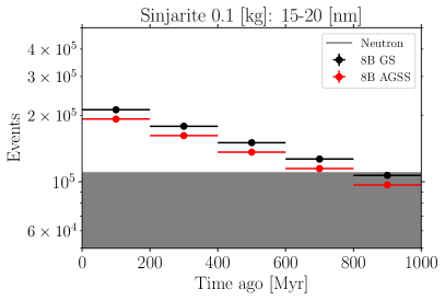
Figure 7: Same as Fig. 4, but including hydrogen induced tracks and summed over a narrower track lengths of 15–20 nm.

We show the time evolution for sinjarite including its hydrogen induced track contribution, using only 15–20 nm in Fig. 7. We can see that compared to Fig. 4, the signal becomes smaller than the background as early as $\sim 800$ Myr. If instead we continue to use 15–30 nm, the signal becomes smaller than the background already by $\sim 200$ Myr.

References

- Usoskin (2008) I. G. Usoskin, Living Rev. Sol. Phys. 5, 3 (2008), arXiv:0810.3972 [astro-ph] .
- Bond et al. (2001) G. Bond, B. Kromer, J. Beer, R. Muscheler, M. N. Evans, W. Showers, S. Hoffmann, R. Lotti-Bond, I. Hajdas, and G. Bonani, Science 294, 2130 (2001).
- Beer et al. (2000) J. Beer, W. Mende, and R. Stellmacher, Quaternary Science Reviews 19, 403 (2000).
- Ribas et al. (2005) I. Ribas, E. F. Guinan, M. Gudel, and M. Audard, The Astrophysical Journal 622, 680 (2005).
- Bahcall et al. (1968) J. N. Bahcall, N. A. Bahcall, and G. Shaviv, Phys. Rev. Lett. 20, 1209 (1968).
- Haxton et al. (2013a) W. Haxton, R. Hamish Robertson, and A. M. Serenelli, Annual Review of Astronomy and Astrophysics 51, 21 (2013a).
- Pontecorvo (1968) B. Pontecorvo, Sov. Phys. JETP 26, 984 (1968).
- Mikheyev and Smirnov (1985) S. P. Mikheyev and A. Y. Smirnov, Sov. J. Nucl. Phys. 42, 913 (1985).
- Wolfenstein (1979) L. Wolfenstein, Phys. Rev. D 20, 2634 (1979).
- Wolfenstein (1978) L. Wolfenstein, Phys. Rev. D 17, 2369 (1978).
- Mikheev and Smirnov (1986) S. P. Mikheev and A. Y. Smirnov, Nuovo Cim. C 9, 17 (1986).
- Ahmad et al. (2002) Q. R. Ahmad, R. C. Allen, T. C. Andersen, J. D.Anglin, J. C. Barton, E. W. Beier, M. Bercovitch, J. Bigu, S. D. Biller, R. A. Black, I. Blevis, R. J. Boardman, J. Boger, E. Bonvin, M. G. Boulay, M. G. Bowler, T. J. Bowles, S. J. Brice, M. C. Browne, T. V. Bullard, G. Bühler, J. Cameron, Y. D. Chan, H. H. Chen, M. Chen, X. Chen, B. T. Cleveland, E. T. H. Clifford, J. H. M. Cowan, D. F. Cowen, G. A. Cox, X. Dai, F. Dalnoki-Veress, W. F. Davidson, P. J. Doe, G. Doucas, M. R. Dragowsky, C. A. Duba, F. A. Duncan, M. Dunford, J. A. Dunmore, E. D. Earle, S. R. Elliott, H. C. Evans, G. T. Ewan, J. Farine, H. Fergani, A. P. Ferraris, R. J. Ford, J. A. Formaggio, M. M. Fowler, K. Frame, E. D. Frank, W. Frati, N. Gagnon, J. V. Germani, S. Gil, K. Graham, D. R. Grant, R. L. Hahn, A. L. Hallin, E. D. Hallman, A. S. Hamer, A. A. Hamian, W. B. Handler, R. U. Haq, C. K. Hargrove, P. J. Harvey, R. Hazama, K. M. Heeger, W. J. Heintzelman, J. Heise, R. L. Helmer, J. D. Hepburn, H. Heron, J. Hewett, A. Hime, M. Howe, J. G. Hykawy, M. C. P. Isaac, P. Jagam, N. A. Jelley, C. Jillings, G. Jonkmans, K. Kazkaz, P. T. Keener, J. R. Klein, A. B. Knox, R. J. Komar, R. Kouzes, T. Kutter, C. C. M. Kyba, J. Law, I. T. Lawson, M. Lay, H. W. Lee, K. T. Lesko, J. R. Leslie, I. Levine, W. Locke, S. Luoma, J. Lyon, S. Majerus, H. B. Mak, J. Maneira, J. Manor, A. D. Marino, N. McCauley, A. B. McDonald, D. S. McDonald, K. McFarlane, G. McGregor, R. Meijer Drees, C. Mifflin, G. G. Miller, G. Milton, B. A. Moffat, M. Moorhead, C. W. Nally, M. S. Neubauer, F. M. Newcomer, H. S. Ng, A. J. Noble, E. B. Norman, V. M. Novikov, M. O’Neill, C. E. Okada, R. W. Ollerhead, M. Omori, J. L. Orrell, S. M. Oser, A. W. P. Poon, T. J. Radcliffe, A. Roberge, B. C. Robertson, R. G. H. Robertson, S. S. E. Rosendahl, J. K. Rowley, V. L. Rusu, E. Saettler, K. K. Schaffer, M. H. Schwendener, A. Schülke, H. Seifert, M. Shatkay, J. J. Simpson, C. J. Sims, D. Sinclair, P. Skensved, A. R. Smith, M. W. E. Smith, T. Spreitzer, N. Starinsky, T. D. Steiger, R. G. Stokstad, L. C. Stonehill, R. S. Storey, B. Sur, R. Tafirout, N. Tagg, N. W. Tanner, R. K. Taplin, M. Thorman, P. M. Thornewell, P. T. Trent, Y. I. Tserkovnyak, R. Van Berg, R. G. Van de Water, C. J. Virtue, C. E. Waltham, J.-X. Wang, D. L. Wark, N. West, J. B. Wilhelmy, J. F. Wilkerson, J. R. Wilson, P. Wittich, J. M. Wouters, and M. Yeh (SNO Collaboration), Phys. Rev. Lett. 89, 011301 (2002).
- McDonald (2016) A. B. McDonald, Rev. Mod. Phys. 88, 030502 (2016).
- Wurm (2017) M. Wurm, Phys. Rept. 685, 1 (2017), arXiv:1704.06331 [hep-ex] .
- Degl’Innocenti et al. (1997) S. Degl’Innocenti, W. Dziembowski, G. Fiorentini, and B. Ricci, Astropart. Phys. 7, 77 (1997), arXiv:astro-ph/9612053 .
- Gough et al. (1996) D. Gough et al., Science 272, 1296 (1996).
- Mitalas and Sills (1992) R. Mitalas and K. R. Sills, Astrophys. J. 401, 759 (1992).
- Asplund et al. (2009) M. Asplund, N. Grevesse, A. Sauval, and P. Scott, Ann. Rev. Astron. Astrophys. 47, 481 (2009), arXiv:0909.0948 [astro-ph.SR] .
- Grevesse and Sauval (1998) N. Grevesse and A. J. Sauval, Space Sci. Rev. 85, 161 (1998).
- Serenelli et al. (2009) A. M. Serenelli, S. Basu, J. W. Ferguson, and M. Asplund, The Astrophysical Journal 705, L123 (2009).
- Serenelli et al. (2011) A. M. Serenelli, W. C. Haxton, and C. Peña-Garay, The Astrophysical Journal 743, 24 (2011).
- Drukier et al. (2019) A. K. Drukier, S. Baum, K. Freese, M. Górski, and P. Stengel, Phys. Rev. D 99, 043014 (2019).
- Edwards et al. (2019a) T. D. P. Edwards, B. J. Kavanagh, C. Weniger, S. Baum, A. K. Drukier, K. Freese, M. Górski, and P. Stengel, Phys. Rev. D 99, 043541 (2019a).
- Edwards et al. (2019b) T. D. Edwards, B. J. Kavanagh, C. Weniger, S. Baum, A. K. Drukier, K. Freese, M. Górski, and P. Stengel, Phys. Rev. D 99, 043541 (2019b), arXiv:1811.10549 [hep-ph] .
- Baum et al. (2020a) S. Baum, A. K. Drukier, K. Freese, M. Górski, and P. Stengel, Physics Letters B 803, 135325 (2020a).
- Baum et al. (2020b) S. Baum, T. D. P. Edwards, B. J. Kavanagh, P. Stengel, A. K. Drukier, K. Freese, M. Górski, and C. Weniger, Phys. Rev. D 101, 103017 (2020b).
- Jordan et al. (2020) J. R. Jordan, S. Baum, P. Stengel, A. Ferrari, M. C. Morone, P. Sala, and J. Spitz, Phys. Rev. Lett. 125, 231802 (2020), arXiv:2004.08394 [hep-ph] .
- Bahcall and Ulmer (1996) J. N. Bahcall and A. Ulmer, Phys. Rev. D 53, 4202 (1996), arXiv:astro-ph/9602012 .
- Paxton et al. (2011) B. Paxton, L. Bildsten, A. Dotter, F. Herwig, P. Lesaffre, and F. Timmes, Astrophys. J. Suppl. 192, 3 (2011), arXiv:1009.1622 [astro-ph.SR] .
- Paxton et al. (2013) B. Paxton et al., Astrophys. J. Suppl. 208, 4 (2013), arXiv:1301.0319 [astro-ph.SR] .
- Paxton et al. (2015) B. Paxton et al., Astrophys. J. Suppl. 220, 15 (2015), arXiv:1506.03146 [astro-ph.SR] .
- Paxton et al. (2018) B. Paxton et al., Astrophys. J. Suppl. 234, 34 (2018), arXiv:1710.08424 [astro-ph.SR] .
- Paxton et al. (2019) B. Paxton, R. Smolec, J. Schwab, A. Gautschy, L. Bildsten, M. Cantiello, A. Dotter, R. Farmer, J. A. Goldberg, A. S. Jermyn, S. M. Kanbur, P. Marchant, A. Thoul, R. H. D. Townsend, W. M. Wolf, M. Zhang, and F. X. Timmes, 243, 10 (2019), arXiv:1903.01426 [astro-ph.SR] .
- Farag et al. (2020) E. Farag, F. X. Timmes, M. Taylor, K. M. Patton, and R. Farmer, The Astrophysical Journal 893, 133 (2020).
- Bouvier and Wadhwa (2010) A. Bouvier and M. Wadhwa, Nature Geoscience 3, 637 (2010).
- Prša et al. (2016) A. Prša, P. Harmanec, G. Torres, E. Mamajek, M. Asplund, N. Capitaine, J. Christensen-Dalsgaard, E. Depagne, M. Haberreiter, S. Hekker, and et al., The Astronomical Journal 152, 41 (2016).
- Villante et al. (2014) F. L. Villante, A. M. Serenelli, F. Delahaye, and M. H. Pinsonneault, Astrophys. J. 787, 13 (2014), arXiv:1312.3885 [astro-ph.SR] .
- Haxton et al. (2013b) W. Haxton, R. Hamish Robertson, and A. M. Serenelli, Ann. Rev. Astron. Astrophys. 51, 21 (2013b), arXiv:1208.5723 [astro-ph.SR] .
- Bellini et al. (2011) G. Bellini et al., Phys. Rev. Lett. 107, 141302 (2011), arXiv:1104.1816 [hep-ex] .
- Agostini et al. (2020) M. Agostini et al. (BOREXINO), Nature 587, 577 (2020), arXiv:2006.15115 [hep-ex] .
- ILIA and DURRANI (2003) R. ILIA and S. A. DURRANI, in Handbook of Radioactivity Analysis (Second Edition), edited by M. F. L’Annunziata (Academic Press, San Diego, 2003) second edition ed., pp. 179 – 237.
- Mei and Hime (2006) D. Mei and A. Hime, Phys. Rev. D 73, 053004 (2006), arXiv:astro-ph/0512125 .
- Bowes (1990) D. R. Bowes, “Ultrabasic igneous rocksultrabasic igneous rocks,” in Petrology (Springer US, Boston, MA, 1990) pp. 576–577.
- Dean (2013) W. E. Dean, “Marine evaporites,” in Encyclopedia of Marine Geosciences, edited by J. Harff, M. Meschede, S. Petersen, and J. Thiede (Springer Netherlands, Dordrecht, 2013) pp. 1–10.
- Ziegler et al. (2010) J. F. Ziegler, M. Ziegler, and J. Biersack, Nuclear Instruments and Methods in Physics Research Section B: Beam Interactions with Materials and Atoms 268, 1818 (2010), 19th International Conference on Ion Beam Analysis.
- Wilson et al. (2005) W. B. Wilson, R. T. Perry, W. S. Charlton, T. A. Parish, and E. F. Shores, Radiation Protection Dosimetry 115, 117 (2005), https://academic.oup.com/rpd/article-pdf/115/1-4/117/4540829/nci260.pdf .
- Madland et al. (1999) D. G. Madland, E. D. Arthur, G. P. Estes, J. E. Stewart, M. Bozoian, R. T. Perry, T. A. Parish, T. H. Brown, T. R. England, W. B. Wilson, and W. S. Charlton, (1999), 10.2172/15215.
- Honda et al. (2011) M. Honda, T. Kajita, K. Kasahara, and S. Midorikawa, Phys. Rev. D 83, 123001 (2011).
- O’Hare (2016) C. A. O’Hare, Phys. Rev. D 94, 063527 (2016), arXiv:1604.03858 [astro-ph.CO] .
- Gallagher et al. (1998) K. Gallagher, R. Brown, and C. Johnson, Annual Review of Earth and Planetary Sciences 26, 519 (1998), https://doi.org/10.1146/annurev.earth.26.1.519 .