A 3D radiative transfer framework: XII. Many-core, vector and GPU methods

Abstract

3D detailed radiative transfer is computationally taxing, since the solution of the radiative transfer equation involves traversing the six dimensional phase space of the 3D domain. With modern supercomputers the hardware available for wallclock speedup is rapidly changing, mostly in response to requirements to minimize the cost of electrical power. Given the variety of modern computing architectures, we aim to develop and adapt algorithms for different computing architectures to improve performance on a wide variety of platforms. We implemented the main time consuming kernels for solving 3D radiative transfer problems for vastly different computing architectures using MPI, OpenMP, OpenACC and vector algorithms. Adapted algorithms lead to massively improved speed for all architectures, making extremely large model calculations easily feasible. These calculations would have previously been considered impossible or prohibitively expensive. Efficient use of modern computing devices is entirely feasible, but unfortunately requires the implementation of specialized algorithms for them.

1 Introduction

In a series of papers, we have described a framework for solving the radiative transfer equation in 3D systems (3DRT), including a detailed treatment of scattering in continua and lines with a non local operator splitting method and its use in the general model atmosphere package PHOENIX [1, 2, 3, 4, 5, 6, 7, 8, 9, 10, 11, hereafter: Papers I–XI].

We give a short summary of the problem and the numerical approach in the next section.

In typical non-local thermodynamic equilibrium (NLTE) PHOENIX/3D applications, the 3DRT uses about 75% of the overall compute time, that is, reducing the time consumed by the 3DRT module will significantly reduce the overall simulation time. This is an advantage of our approach since only a small subset of code modules require specialized directives and code modifications to match the targeted hardware and compiler.

In Paper VIII [8] we showed that specialized codes for GPUs can result in significantly improved performance compared to standard CPUs of the era. With the availability of new many-core CPUs (e.g., Intel Phi), vector CPUs (i.e., NEC Aurora TSUBASA) and GPUs, the need for algorithms specially adapted to the hardware in order to maximize performance on such systems becomes apparent. This becomes more urgent due the fact that modern supercomputers are being built using many-core CPUs or as hybrid CPU/GPU systems. While, it is likely that efficient use of such systems will require specialized algorithms, it is not economical to design special codes for each system or to use vendor-locked programming models as individual computing system lifetimes (5 years) are typically much shorter than code lifetimes (20+ years).

For these reasons, we investigate here how 3D radiative transfer calculations can be accelerated using algorithms adapted to many-core and vector CPUs as well as to GPUs. As codes will be used potentially for decades, it is very important to adhere to general standards as closely as possibly in order to retain source code compatibility for long time scales. Thus, we will use Fortran 2008 [12] as the base programming language and will use MPI [13], OpenMP [14] and OpenACC [15] as additional directive based performance enhancers. In addition, directive based statements for specific systems, e.g., to vectorize loops, are considered as long as they do not interfere with portability to other systems.

In the following, we consider two test cases that represent typical 3DRT usage patterns of PHOENIX/3D: A Cartesian box with periodic boundary conditions in the horizontal (x,y) plane and a spherical coordinate system case used in irradiation models in pre-CVs or exoplanets. These general setups cover the vast majority of current and planned PHOENIX/3D calculations, accelerating them can save millions of CPU-core-hours and related energy expenditures. In addition, faster calculations can enable the use of smaller supercomputers so that not only Tier 0 systems, but also Tier 1 or 2 systems can be used for a given model. This can drastically reduce the turnaround time for a model and in turn, free up Tier 0 systems for larger model runs.

2 3D radiative transfer framework

We use a Cartesian or spherical coordinates grid of non-equal sized volume cells (voxels) for the following discussion. The values of physical quantities, such as temperatures, opacities and mean intensities, are averages over a voxel, which, therefore, also fixes the local physical resolution of the grid. In the following we will specify the size of the voxel grid by the number of voxels along each positive axis, e.g., $n_{x}=n_{y}=n_{z}=32$ specifies a voxel grid from voxel coordinates $(-32,-32,-32)$ to $(32,32,32)$ for a total of $(2*32+1)^{3}=274625$ voxels, $65$ along each axis.

The 3DRT framework is typically applied to optically thick environments with a significant scattering contribution, e.g., modeling the light reflected by an extrasolar giant planet close to its parent star. Therefore, not only a formal solution (see below) of the radiative transfer equation is required, but the full solution of the 3D radiative transfer equation with scattering. The fundamental numerical method used in the 3DRT framework is an operator splitting approach. Operator splitting works best if a non-local ${\Lambda^{*}}$ operator is used in the calculations [e.g., 16], therefore, we exclusively use a non-local ${\Lambda^{*}}$ method.

2.1 Radiative transfer equation

For simplicity, we consider here only the static, steady-state radiative transfer equation in 3D (see [9, 10] for the non-static case) written as

$$\hat{\vec{n}}\cdot\nabla I(\nu,\vec{x},\hat{\vec{n}})=\eta(\nu,\vec{x})-\chi(\nu,\vec{x})I(\nu,\vec{x},\hat{\vec{n}})$$ (1)

where $I(\nu,\vec{x},\hat{\vec{n}})$ is the specific intensity at frequency $\nu$, position $\vec{x}$, in the direction $\hat{\vec{n}}$, $\eta(\nu,\vec{x})$ is the emissivity at frequency $\nu$ and position $\vec{x}$, and $\chi(\nu,\vec{x})$ is the total extinction at frequency $\nu$ and position $\vec{x}$. The source function $S={\eta}/{\chi}$. Mathematically, this is a linear first order partial intro-differential equation. In Cartesian coordinates the $\nabla=\frac{\partial}{\partial x}+\frac{\partial}{\partial y}+\frac{\partial}{\partial z}$ and the direction $\hat{\vec{n}}$ is defined by two angles $(\theta,\phi)$ at the position $\vec{x}$.

2.2 The operator splitting method

The mean intensity $J$ is obtained from the source function $S$ by a formal solution of the RTE which is symbolically written using the $\Lambda$-operator $\Lambda$ as

$$J=\Lambda S.$$ (2)

The source function is given by $S=(1-\epsilon)J+\epsilon B$, where $\epsilon$ denotes the thermal coupling parameter and $B$ is Planck’s function.

The $\Lambda$-iteration method, i.e. to solve Eq. 2 by a fixed-point iteration scheme of the form

$${\bar{J}_{\rm new}}=\Lambda{S_{\rm old}},\quad{S_{\rm new}}=(1-\epsilon){\bar{J}_{\rm new}}+\epsilon B,$$ (3)

fails in the case of large optical depths and small $\epsilon$.

Here, ${\bar{J}}=\int_{0}^{\infty}J_{\lambda}\phi_{\lambda}\,d\lambda$ is the mean intensity averaged over the line profile, $\phi_{\lambda}$; ${S_{\rm old}}$ is the current estimate for the source function $S$; and ${S_{\rm new}}$ is the new, improved, estimate of $S$ for the next iteration. The failure of the $\Lambda$-iteration to converge is caused by the fact that the largest eigenvalue of the amplification matrix is approximately [17] $\lambda_{\rm max}\approx(1-\epsilon)(1-T^{-1})$, where $T$ is the optical thickness of the medium. For small $\epsilon$ and large $T$, this is very close to unity and, therefore, the convergence rate of $\Lambda$-iteration is very poor. A physical description of this effect can be found in [18].

The idea of the operator splitting (OS) method is to reduce the eigenvalues of the amplification matrix in the iteration scheme [19] by introducing an approximate $\Lambda$-operator (ALO) ${\Lambda^{*}}$ and to split $\Lambda$ according to

$$\Lambda={\Lambda^{*}}+(\Lambda-{\Lambda^{*}})$$ (4)

and rewrite Eq. 3 as

$${\bar{J}_{\rm new}}={\Lambda^{*}}{S_{\rm new}}+(\Lambda-{\Lambda^{*}}){S_{\rm old}}.$$ (5)

This relation can be written as [20]

$$\left[1-{\Lambda^{*}}(1-\epsilon)\right]{\bar{J}_{\rm new}}={\bar{J}_{\rm fs}}-{\Lambda^{*}}(1-\epsilon){\bar{J}_{\rm old}},$$ (6)

where ${\bar{J}_{\rm fs}}=\Lambda{S_{\rm old}}$ and ${\bar{J}_{\rm old}}$ is the current estimate of the mean intensity $J$. Equation 6 is solved to get the new values of ${\bar{J}}$ which is then used to compute the new source function for the next iteration cycle. The calculation and the structure of ${\Lambda^{*}}$ should be simple in order to make the construction of the linear system in Eq. 6 fast. For example, the choice ${\Lambda^{*}}=\Lambda$ is best in view of the convergence rate (it is equivalent to a direct solution by matrix inversion) but the explicit construction of $\Lambda$ is more time consuming than the construction of a simpler ${\Lambda^{*}}$.

The CPU time required for the solution of the RTE using the OS method depends on several factors: (a) the time required for a formal solution and the computation of ${\bar{J}_{\rm fs}}$, (b) the time needed to construct ${\Lambda^{*}}$, (c) the time required for the solution of Eq. 6, and (d) the number of iterations required for convergence to the prescribed accuracy.

3 Test cases

The basic test setups for the Cartesian grid with periodic boundary conditions (PBCs) and the spherical coordinate system (SP) were chosen so that the tests can run on the smallest memory system (GPU) that we used here. These setups are the basic building blocks that are employed in more complex models (e.g., 3D NLTE calculations).

3.1 Test case setup: periodic boundary conditions

The test cases we have investigated follow the continuum tests used in [3] and [8]. In detail, we used a configuration that utilizes periodic boundary conditions (PBCs) in a plane parallel slab. We used PBCs on the $x$ and $y$ axes, $z_{\rm max}$ is the outside boundary, and $z_{\rm min}$ the inside boundary. The slab has a finite optical depth in the $z$ axis. The basic model parameters are

1. the total thickness of the slab, $z_{\rm max}-z_{\rm min}=10^{8}\,$cm;

2. the minimum optical depth in the continuum, $\tau_{\rm std}^{\rm min}=10^{-4}$ and the maximum optical depth in the continuum, $\tau_{\rm std}^{\rm max}=10^{8}$;

3. grey temperature structure for $\hbox{$\,T_{\rm eff}$}=10^{4}$ K;

4. boundary conditions with outer boundary condition $I_{\rm bc}^{-}\equiv 0$ and inner boundary condition LTE diffusion;

5. parameterized coherent and isotropic continuum scattering given by

   $$\chi_{c}=\epsilon_{c}\kappa_{c}+(1-\epsilon_{c})\sigma_{c}$$

   with $\epsilon_{c}=10^{-2}$. $\kappa_{c}$ and $\sigma_{c}$ are the continuum absorption and scattering coefficients.

The Cartesian grid has $(n_{x},n_{y},n_{z})=(65,65,257)=1085825$ voxels and we use $\Omega=(n_{\theta},n_{\phi})=(32,16)=512$ solid angles for the formal solution, equally spaced in $\mu=\cos(\theta)$ and $\phi$.

3.2 Test case setup: spherical coordinate system

The setup for the spherical coordinate system test (SP) follows the general setup for the corresponding case in Paper IV [4]. The configuration used here is:

1. Inner radius $r_{c}=10^{10}\,$cm, outer radius $\hbox{$r_{\rm out}$}=2\times 10^{10}\,$cm.

2. Minimum optical depth in the continuum $\tau_{\rm std}^{\rm min}=10^{-8}$ and maximum optical depth in the continuum $\tau_{\rm std}^{\rm max}=10^{1}$.

3. Grey temperature structure with $\hbox{$\,T_{\rm eff}$}=10^{4}$ K.

4. Outer boundary condition $I_{\rm bc}^{-}\equiv 0$ and diffusion inner boundary condition.

5. Continuum extinction $\chi_{c}=C/r^{6}$, with the constant $C$ fixed by the radius and optical depth grids.

6. Parameterized coherent and isotropic continuum scattering by defining

   $$\chi_{c}=\epsilon_{c}\kappa_{c}+(1-\epsilon_{c})\sigma_{c}$$

   with $\epsilon_{c}=10^{-2}$. $\kappa_{c}$ and $\sigma_{c}$ are the continuum absorption and scattering coefficients.

The spherical grid (SP) has $(n_{r},n_{\theta},n_{\phi})=(129,33,65)=276705$ voxels and we use $\Omega=(n_{\theta},n_{\phi})=(8,16)=128$ solid angles for the formal solution (equally spaced in $\mu=\cos(\theta)$ and $\phi$. This is smaller than in typical PHOENIX/3D applications, however, this setup still fits into the smallest RAM of the test systems. The timing profile of this setup is similar to large scale PHOENIX/3D runs, so that we use it as a model in this work.

3.3 Test systems

3.3.1 CPU: Intel Xeon

The base system for the comparison is a dual Intel Xeon CPU W-3223 with 3.50GHz clock-speed at 8 cores per CPU and 2 hardware threads per core. The system is realized in a MacPro7,1 system with 96GB RAM. The OS is MacOS 10.15, the available compilers are GCC 10.2.0, Intel 19.1.3.301 and PGI 19.10-0 (the newer NVIDIA HPC compilers were not available for MacOS).

3.3.2 GPU: NVIDIA V100

The GPU test system is a 8 core Xeon Silver 4110 (Skylake) 2.1GHz host machine with a NVIDIA V100 GPU with 32GB RAM. The GPU has a clock speed of 1380 MHz and a Memory Clock Rate of 877 MHz and 4096 bits memory bus width. To target the GPU, we use OpenACC as implemented in the NVIDIA Fortran compiler version 20.9-0. The host system is running Centos 7. For the host CPU the Intel compiler version 19.1.3.304 is also available.

3.3.3 Many-core: KNL

The many-core test system is a Intel Xeon Phi CPU 7250 (Knights Landing; KNL) based system with 1.30GHz clock speed, 64 cores and 4 hardware threads per core, similar to the NERSC Cori nodes (https://www.nersc.gov/users/computational-systems/cori/). On this system with use Intel compiler version 19.1.3.304 with OpenMP directives turned on.

3.3.4 Vector: NEC SX-Aurora TSUBASA

As a vector processor test system we use a NEC SX-Aurora TSUBASA A101 (Aurora) machine with 2 vector engine (VE) cards. Each card has 48GB RAM, 8 vector cores at 1.4 GHz clock speed. The vector host (VH) is a Xeon Gold 6126 CPU (Skylake) at 2.60GHz clock-speed with 96GB RAM. The VH manages the 2 VEs and handles their I/O requests, runs the compiler etc. The (MPI) application runs completely on the VEs and is natively compiled using the NEC Fortran compiler, version 2.1.1. The VE have fast vector pipelines and a scalar unit on each core. For the test we use the NEC Fortran Compiler to create vectorized executables with the help of compiler directives and NEC MPI for the MPI based parallelization.

In addition to the VE, the VH can also be used for calculations. We thus ran tests with the Intel Fortran Compiler (version 19.1.3.304) and the NVIDIA compiler (version 20.9-0) with their respective MPI and OpenMP implementations.

4 Method

In the following discussion we use the notation of Papers I – XI.

Considering the 3DRT module individually for any given wavelength, the biggest time consumers are: setting up the geometric paths through the grid for all solid angles (henceforth: the tracker), computing the formal solution for all solid angles, computing the ${\Lambda^{*}}$ operator (only in the first iteration) and the operator splitting solver (computing the new $J$’s by solving the operator splitting linear system, see Paper I). In addition, MPI load balancing may be measurable (e.g., if the workload for different solid angles is significantly different so that some MPI processes finish faster than others, this is the case in the PBC test setup). These steps are repeated for all wavelength points that are considered in a calculation.

For the solution of the large sparse linear system (its rank is equal to the total number of voxels of the simulation) in the operator splitting step (‘OS iteration’) we have implemented 3 algorithms: a Jacobi iteration, a Gauss-Seidel iteration, and the BiCGStab method [21], parallelized with MPI, OpenMP and OpenACC. Each of them performs differently on the test systems and we show in the graphs the fastest version for each of the test runs.

The standard algorithm implements the algorithms described in Paper III (PBCs) and IV (SP) for multi-CPU systems with MPI parallelization: In the formal solution (and ${\Lambda^{*}}$ computation) different solid angles are parallelized and the data needs to be collected from all participating processes only at the end of the formal solution. Similarly, the operator splitting step is parallelized with MPI. The standard algorithm was designed to minimize the memory footprint, so that calculations can be performed on smaller machines. One important observation is that the tracker and the formal solution are memory, rather than compute bound: The different solid angles cause memory access patterns that are aligned with optimal memory and cache access patterns only in specific cases — in most cases memory is accessed randomly through the formal solution. Thus, memory latency is the primary bottleneck.

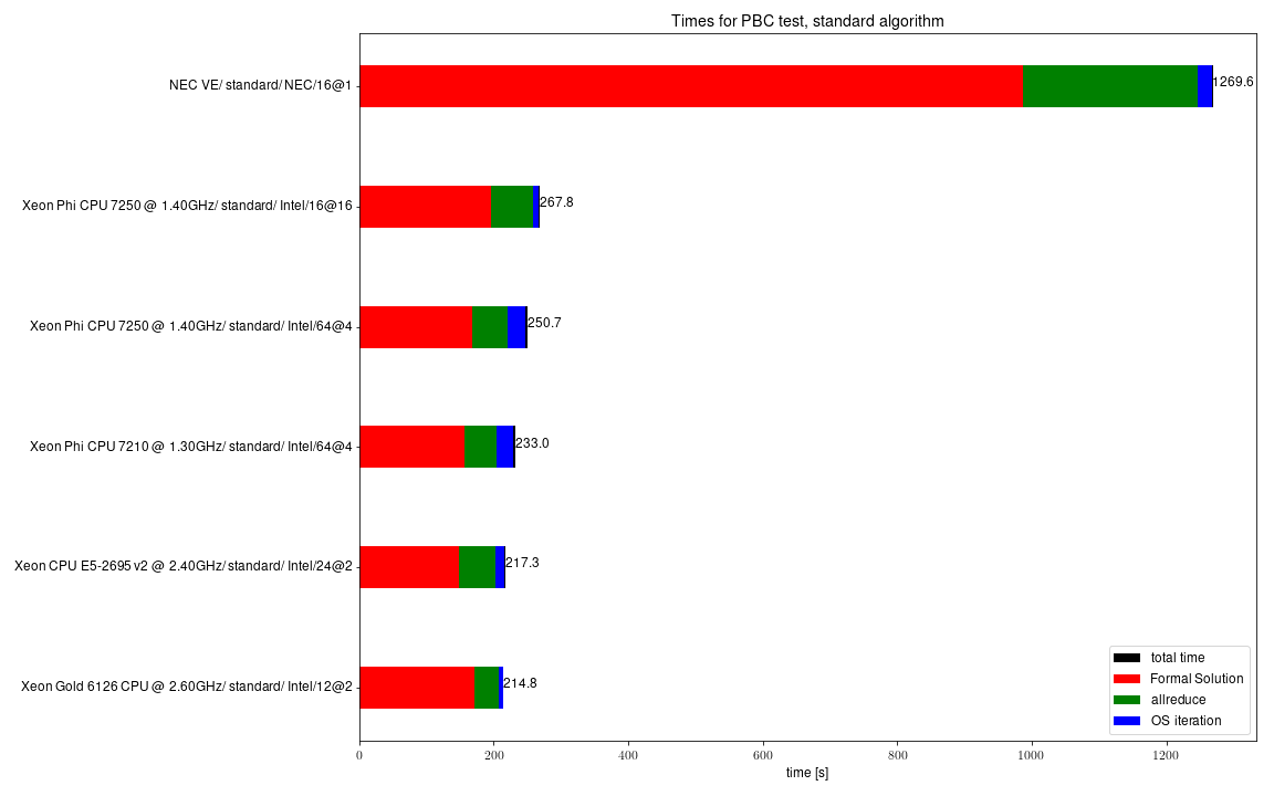
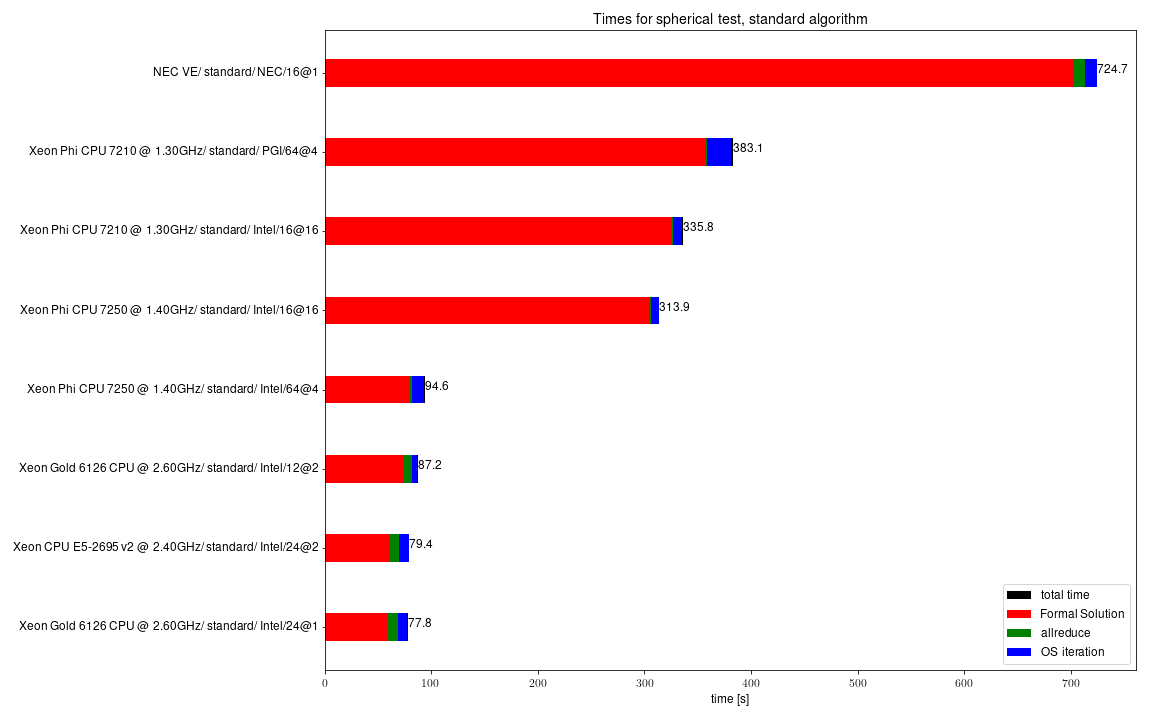
Figure 1: Timing of the standard algorithm. The horizontal bars give the overall execution walltimes (summed over all iterations) of the different phases of the 3D radiative transfer solver as indicated by the colors. ‘Formal Solution’ designates the phase where new mean intensities are computed from the current estimate of the source function (including the construction of the ${\Lambda^{*}}$ operator in the first iteration), ‘allreduce’ is the phase where the contribution of all MPI processes are collected and summed up via MPI functions and ‘OS iteration’ is the time spent computing the new estimate of the source function (including the solution of the large sparse linear system). The labels on the right hand of the bars give the overall execution time. The labels on the left hand side specify the system or CPU, the algorithm, the solver of the large linear system in the OS step (Jacobi, Gauss-Seidel oder BiCGStab), the compiler and the parallelization setup (where the notation $x$@$y$ indices $x$ MPI processes with $y$ OpenMP thread each).

Some results for the standard algorithm are shown in Fig. 1. The performance on older Skylake (Silver 4110) and newer Cascade Lake (W-3223) CPUs is roughly the same. All times are given for a complete node, i.e., all cores of the CPU(s) of the node are used, a common pattern in High Performance Computing, (HPC). The standard algorithm is not multi-threaded with OpenMP, thus the multiple CPU cores are used with MPI parallelization. For comparison we also include the results on the Intel Xeon Phi KNL many-core CPU and the NEC Aurora vector CPU. Whereas the standard algorithm on the KNL CPU fares very well, its performance on the vector processor is abysmal. This is due to the un-threaded and un-vectorizable form of the standard algorithm. The theoretical performance of the KNL cannot be realized in this setup since the standard algorithm does not produce performance gains with OpenMP threading: It requires critical sections and atomic constructs to give correct results and the memory access pattern causes delays in the OpenMP threads, so that OpenMP directives can even be counter productive.

In the following, we will refer to the “formal solution” as the combination of the formal solution and the the construction of the nearest-neighbor ${\Lambda^{*}}$. Each of these steps, formal solution and ${\Lambda^{*}}$ construction take about the same computation time. In all cases for the standard algorithm, the formal solution takes the largest time (red bars in Fig. 1), whereas the operator splitting solver (blue) timing varies from system to system. The time for the MPI ‘allreduce’ (green) is substantially larger in the PBC case, where the workload between different MPI processes is significantly different, than in the SP model, where the load balancing is much better.

4.1 Many-core algorithm

As a first step towards better performance and constructing an optimized algorithm for the formal solution on many-core CPUs we consider the tracker; in particular, the geometry part. In a typical PHOENIX/3D application, many (100,000 or more) wavelength points are considered for the same structure. NLTE modeling has to repeat this procedure numerous times in order to solve the multi-level NLTE rate equations consistently with the radiation field. Therefore, the geometry and thus, the set of tracks (directions in momentum space) through the voxel grid remain the same for all wavelength points. This can be used to setup and fill a geometry cache once, at the beginning, which is than accessed for all subsequent formal solutions, until the wavelength grid has been traversed. This requires (a) a multi-pass algorithm which separates the geometry tracking from the formal solution and (b) optionally storing the geometry tracking data. This requires substantial additional memory, which is, however, fully distributed over different MPI processes with no communication and sharing required. Thus, when using more MPI processes, each process needs to progressively store less geometry data up to the theoretical limit of one solid angle per MPI process. This situation is actually very realistic in PHOENIX/3D simulations as the domain decomposition requires anywhere from 64 to 1024 MPI processes (typically 4-64 nodes) and in such realistic setups, the geometry cache requires only a small fractional memory increase per MPI process.

The multi-pass algorithm has the additional advantage that it allows for more efficient OpenMP parallelization and Single Instruction Multiple Data (SIMD) style vectorization. Once the geometric paths through the voxel grid are known (either by computing them in a first phase or by recalling them from the geometry cache) for each solid angle, the formal solution can be computed by loops over the voxel grid rather than stepping along each characteristic. To keep the loops short and simple enough for OpenMP based parallelization, it turned out to be advantageous to split the calculation into separate phases. Each phase can then use different OpenMP parallelization and SIMD statement vectorization (for Intel CPUs, using the Intel compilers). This increases memory locality, resulting in better cache usage, but does add temporary arrays that are needed to store intermediate results.

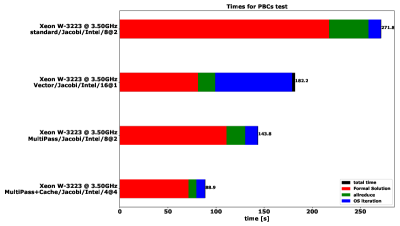
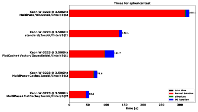
Figure 2: Timing of different algorithms on a modern many-core CPU (Xeon W-3223). The horizontal bars give the overall execution walltimes (summed over all iterations) of the different phases of the 3D radiative transfer solver as indicated by the colors. ‘Formal Solution’ designates the phase where new mean intensities are computed from the current estimate of the source function (including the construction of the ${\Lambda^{*}}$ operator in the first iteration), ‘allreduce’ is the phase where the contribution of all MPI processes are collected and summed up via MPI functions and ‘OS iteration’ is the time spent computing the new estimate of the source function (including the solution of the large sparse linear system). The labels on the right hand of the bars give the overall execution time. The labels on the left hand side specify the system or CPU, the algorithm, the solver of the large linear system in the OS step (Jacobi, Gauss-Seidel oder BiCGStab), the compiler and the parallelization setup (where the notation $x$@$y$ indices $x$ MPI processes with $y$ OpenMP thread each).

For a multi-core CPU the results are shown in Fig. 2, where we use the Xeon W-3223 as an example. Here, the multi-pass algorithm without the geometry cache (labeled ‘MultiPass’ in the figures) performs substantially better than the standard algorithm (about 1.9 times) in the PBC case but substantially worse (by a factor of 2.4) in the SP case. This is caused by the more complex data structures required by the MultiPass algorithm where the geometry tracking phase cannot overlap with the computation phase. However, with the geometry cache active, the results change substantially. Note that in order to simulate the typical results obtained within a larger PHOENIX/3D  model the times do not include the construction of the geometry cache (this is done once before the calculations start). This ‘MultiPassCache’ version produces the best performance for both test cases, about 3 times speedup for the SP case and 2.6 times for the PBC test compared to the standard algorithm. These are substantial speedups on classic multi-core CPUs. Listing 1 gives pseudo-code for this method.

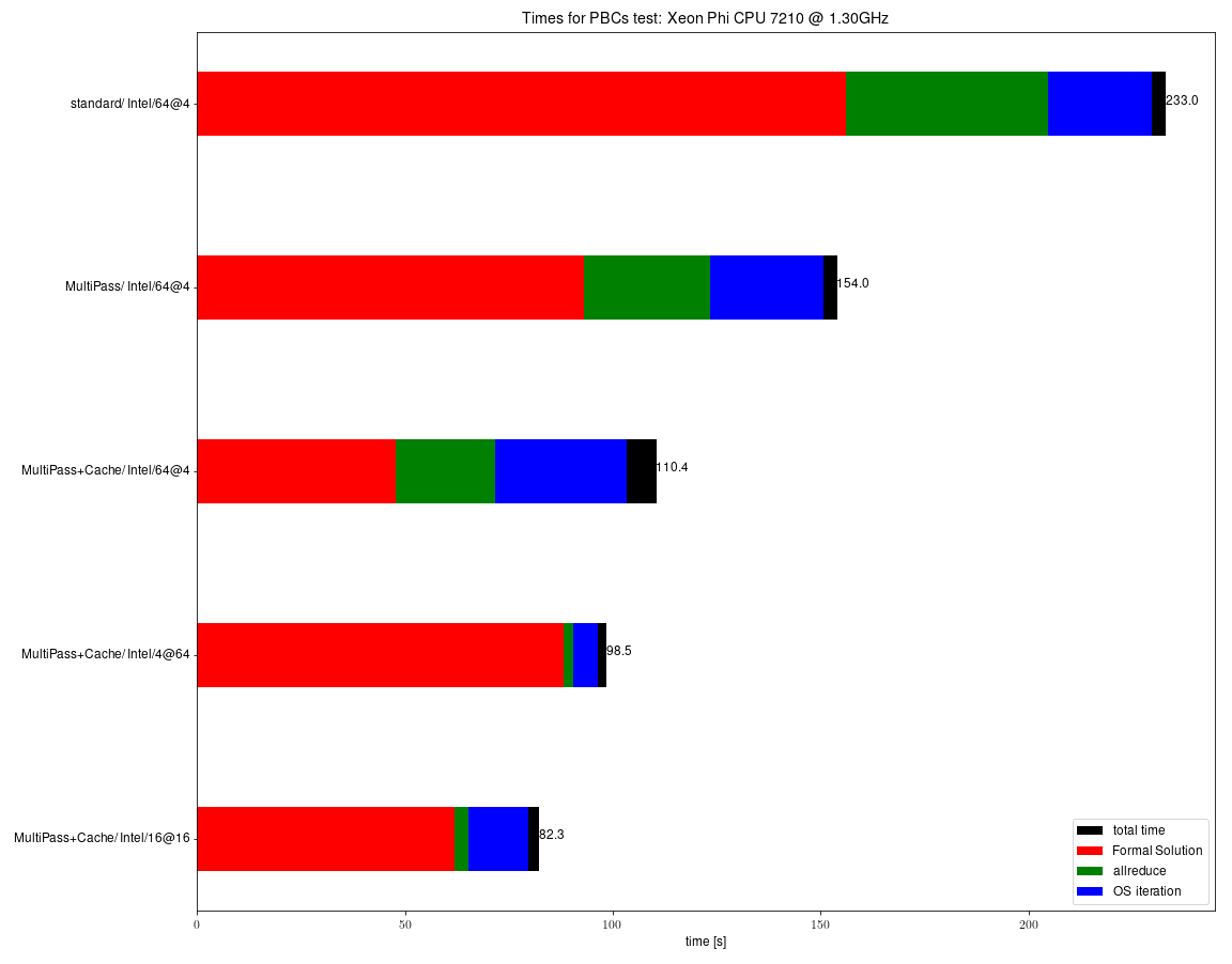
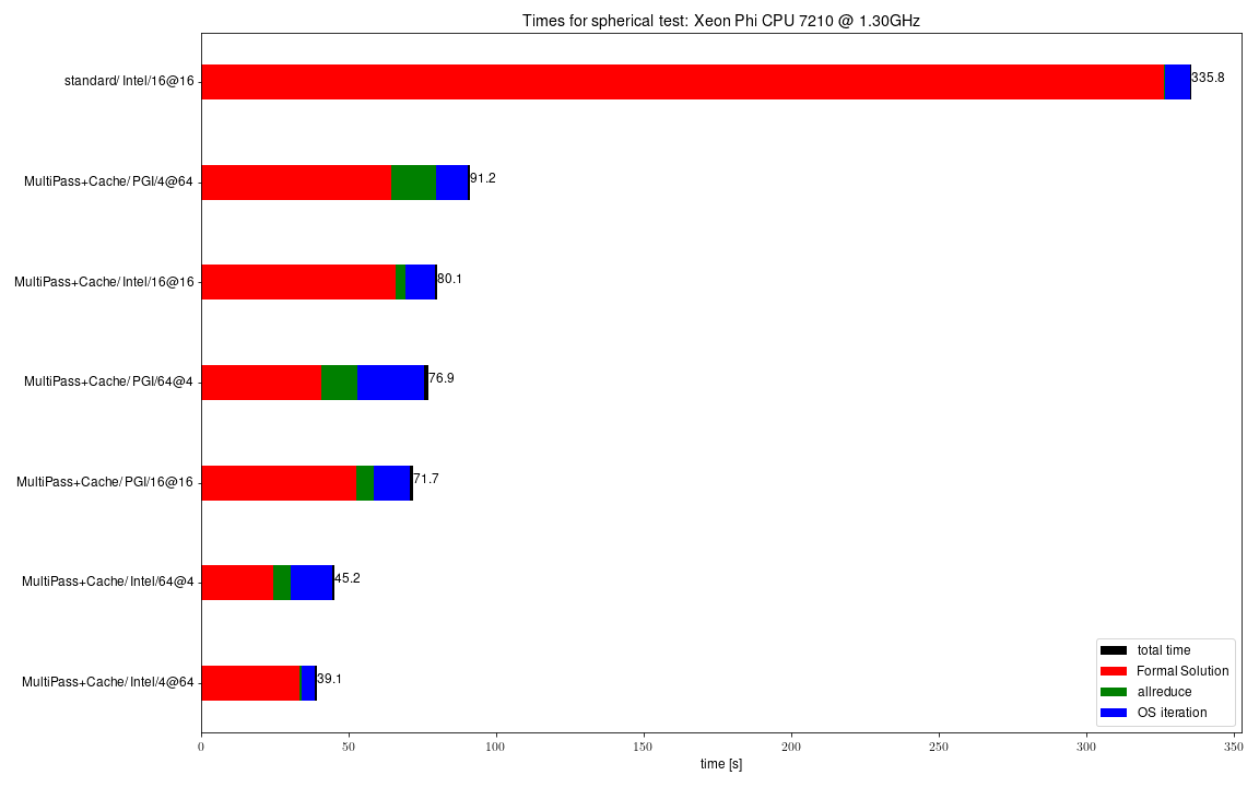
Figure 3: Timing of different algorithms on a many-core CPU (Xeon Phi 7210). The horizontal bars give the overall execution walltimes (summed over all iterations) of the different phases of the 3D radiative transfer solver as indicated by the colors. ‘Formal Solution’ designates the phase where new mean intensities are computed from the current estimate of the source function (including the construction of the ${\Lambda^{*}}$ operator in the first iteration), ‘allreduce’ is the phase where the contribution of all MPI processes are collected and summed up via MPI functions and ‘OS iteration’ is the time spent computing the new estimate of the source function (including the solution of the large sparse linear system). The labels on the right hand of the bars give the overall execution time. The labels on the left hand side specify the system or CPU, the algorithm, the solver of the large linear system in the OS step (Jacobi, Gauss-Seidel oder BiCGStab), the compiler and the parallelization setup (where the notation $x$@$y$ indices $x$ MPI processes with $y$ OpenMP thread each).

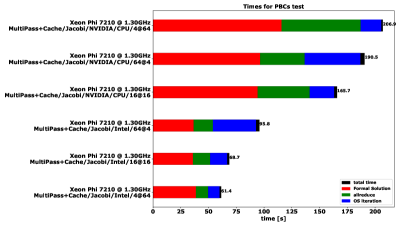
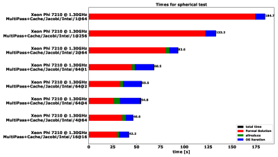
Figure 4: Timing of different MPI+OpenMP setups for the MultiPass+Cache algorithm on a many-core CPU (Xeon Phi 7210). The horizontal bars give the overall execution walltimes (summed over all iterations) of the different phases of the 3D radiative transfer solver as indicated by the colors. ‘Formal Solution’ designates the phase where new mean intensities are computed from the current estimate of the source function (including the construction of the ${\Lambda^{*}}$ operator in the first iteration), ‘allreduce’ is the phase where the contribution of all MPI processes are collected and summed up via MPI functions and ‘OS iteration’ is the time spent computing the new estimate of the source function (including the solution of the large sparse linear system). The labels on the right hand of the bars give the overall execution time. The labels on the left hand side specify the system or CPU, the algorithm, the solver of the large linear system in the OS step (Jacobi, Gauss-Seidel oder BiCGStab), the compiler and the parallelization setup (where the notation $x$@$y$ indices $x$ MPI processes with $y$ OpenMP thread each).

The corresponding results on many-core CPUs are similar. In Figs. 3 and 4 we show the results obtained on the Xeon Phi 7210 (64 cores with 4 hardware threads each at 1.3GHz). Here, the standard algorithm is substantially slower than the ‘MultiPassCache’ setup. The speedups for the MultiPass+Cache version are 3.4 (PBCs) and 2.6 (SP) compared to the standard algorithm. Enabling the geometry cache speeds up the overall calculation by a factor of 2 or more. For a full PHOENIX/3D simulation run this produces massively reduced wallclock times compared to the standard and MultiPass algorithms. In the case of KNL, the MultiPassCache algorithm allows for much better OpenMP utilization, including the OpenMP SIMD statement that is used to vectorize (i.e., use AVX-512 instructions) on the KNL CPU with the Intel compiler. These vectorizations by themselves already produce significant speed-ups compared to the standard algorithm. This result is highlighted by the observation (cf. Fig.  4) that for the SP test on KNL, a 16 MPI processes with 16 OpenMP threads each (16@16) setup, is faster than the more MPI biased 64@4 setup. Even the very openMP focused 4@64 setup is only 10% slower than the 16@16 setup. In the PBC test case, the 4@64 setup is the fastest; however, the 16@16setup is only about 12% slower. This is likely at least, in part, due to MPI load balancing, which is a bigger problem in the PBC test (where the different characteristics have very different lengths in terms of voxel counts than the far more balanced SP test case). These effects show that the KNL is quite sensitive to details of the setup and for each simulation the optimal setup may need to be determined by testing in advance. Experiments using less than the 4 hardware threads per core on KNL (as suggested in some performance documents) reduced performance significantly. It appears that using more threads may be able to hide memory latencies better; however, using more than 4 threads per core also reduced performance.

4.2 Vector processor algorithm

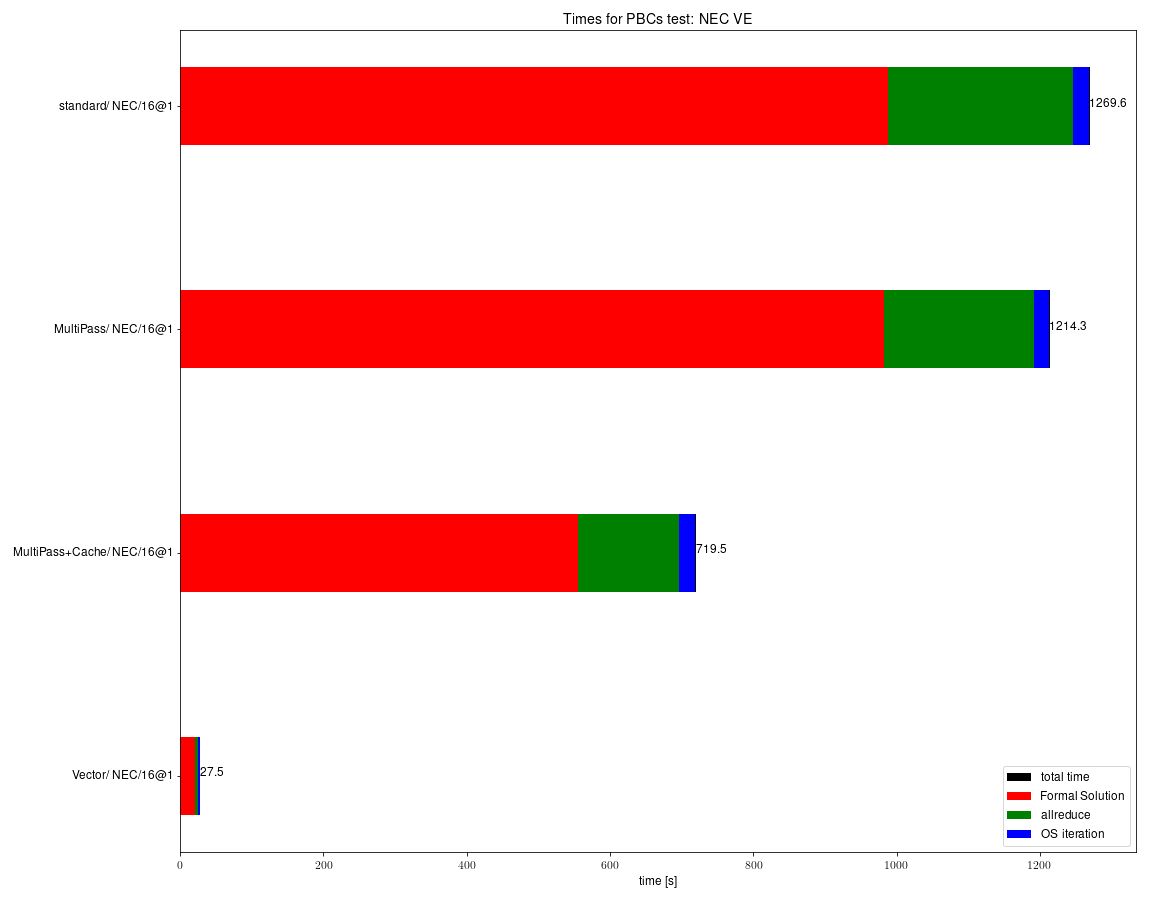
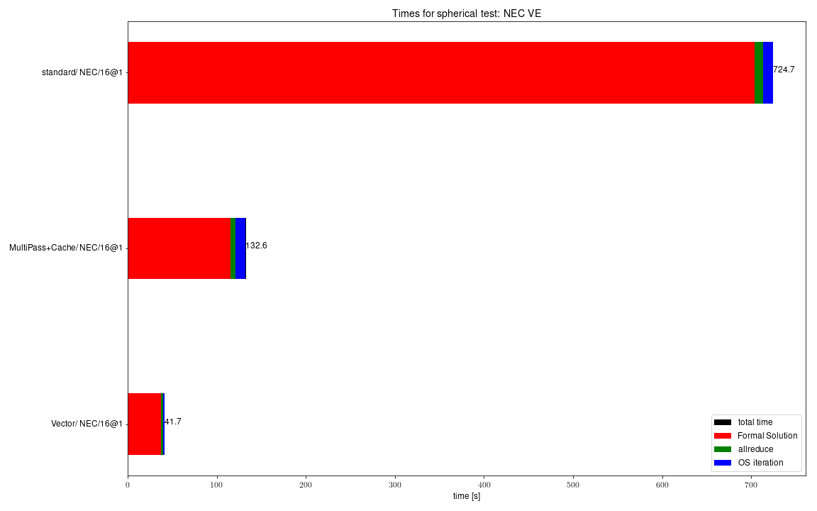
Figure 5: Timing of different algorithms on a vector CPU (NEC SX-Aurora TSUBASA). The horizontal bars give the overall execution walltimes (summed over all iterations) of the different phases of the 3D radiative transfer solver as indicated by the colors. ‘Formal Solution’ designates the phase where new mean intensities are computed from the current estimate of the source function (including the construction of the ${\Lambda^{*}}$ operator in the first iteration), ‘allreduce’ is the phase where the contribution of all MPI processes are collected and summed up via MPI functions and ‘OS iteration’ is the time spent computing the new estimate of the source function (including the solution of the large sparse linear system). The labels on the right hand of the bars give the overall execution time. The labels on the left hand side specify the system or CPU, the algorithm, the solver of the large linear system in the OS step (Jacobi, Gauss-Seidel oder BiCGStab), the compiler and the parallelization setup (where the notation $x$@$y$ indices $x$ MPI processes with $y$ OpenMP thread each).

The Aurora is a vector processor with significantly different performance characteristics than Intel Xeons or many-core CPUs. While its vector performance is very high, its scalar performance is quite low, that is, vectorization is of utmost importance on this system. In Fig. 5 we show the performance results for the standard and MultiPass algorithms, which do not use the vector processing capabilities of the Aurora and the execution times are very long.

Therefore, we have developed a variant of the MultiPass+Cache algorithm that can be vectorized (with directives) by the NEC Fortran compiler. For this, we swapped loop orders (adding intermediate helper arrays where necessary) and split/merged loops so that the NEC compiler vectorized them. The design goal was to vectorize the longest possible loop, even if it requires additional arrays to store intermediate data. The resulting code uses slightly more RAM than the MultiPass+Cache version. In addition, we also developed a vectorized version of the operator splitting solver in order to further increase overall performance. The changes required to the standard operator splitting solvers are small, a few loop rearrangements and vectorization directives.

The performance of the vector algorithm is shown in Fig. 5. Compared to the standard algorithm, the vector version on the Aurora is about 44 times faster for the PBC case and 65 times faster for the SP test case. In addition, the vector version significantly reduces MPI load balance issues. On the multi-core CPU the vector algorithm is 1.5 times faster than the standard algorithm in the PBC case, but only about 17% faster compared to the standard algorithm for the SP test case. On the many-core Xeon Phi, the vector algorithm is 3-4 times slower than the MultiPass+Cache version (not shown). Note that the vector algorithm does not use OpenMP threading, so that, in particular, on KNL, only one thread per core is used. In addition, the Intel compiler does not vectorize the loops in the same way that the NEC compiler does and, therefore, the vector algorithm does not use the Xeon vector instructions (e.g., AVX-512 on the KNL) efficiently.

4.3 GPU (OpenACC) algorithm

Over the last decade, using GPUs to accelerate numerical calculations (compared to classical CPUs) has become important. To enable such usage, proprietary methods [e.g., CUDA, 22] as well as open standards have been developed. The latter are realized both as programming standards, e.g., OpenCL [23], and as (directive based) APIs, e.g., OpenACC [15]. For long term portability and vendor independence, we consider it imperative to utilize an open standard based approach (codes are often used for decades on very different hardware generations). We have published results for OpenCL before [8] and therefore we concentrate here on an OpenACC based approach. New versions of OpenMP also support GPU based offloading; however, the support for available hardware provided by existing compilers that we have access to is presently very limited. Currently, this is actually also true for OpenACC, where the only compiler support available is the NVIDIA compiler [24] on NVIDIA hardware. OpenACC support in GCC [25] was, at the time of this writing, not in an advanced enough state to be usable.

For the OpenACC version we had to make significant changes to the code. The main problem is that OpenACC does not work with the array-of-structures method that the original code (standard, cache, and vector versions) uses. Therefore, we had to redesign the code to also (alternatively) use a structure-of-arrays method (labeled ‘FlatCache’ in the figures) to store the geometry tracking cache and the data used for the operator splitting (e.g., the ${\Lambda^{*}}$ array). On the NEC and the Xeons, the structure-of-arrays version is marginally faster (about 2%) than the array-of-structures method. The individual arrays are then easily transferred onto the GPU with OpenACC update directives. If the GPU device has enough memory, the geometry cache can be stored once on the GPU and then be used directly, without the need to transfer the tracking cache for each solid angle. In the test cases, the caches and additional 3DRT arrays are 25-30GB total, so that they can be stored on the GPU (LargeGPU mode). For comparison, we have also run tests in Small GPU mode where the tracking caches are kept on the host (CPU) and transferred onto the GPU for each solid angle. In this mode, about 1-2GB are used on the GPU so that smaller devices can also be used or multiple processes can be run on one GPU. Note that in MPI mode with several GPUs only a fraction of the tracking cache needs to be stored, thus, proportionally reducing the memory use per GPU.

The OpenACC version of the formal solution is adapted from the vector version by adding OpenACC directives. In a few loops, the order was exchanged to better exploit the GPU architecture.

Listing 2 gives the pseudo-code for this method. The compiler directives are relatively simple and converting from OpenMP to OpenACC is relatively straightforward. Likewise, given a working OpenACC version it is relatively straightforward to port to OpenMP based device directives, based on small test cases that we have been able to evaluate.

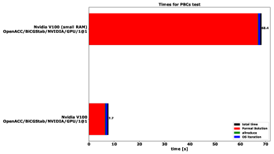
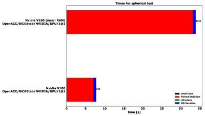
Figure 6: Timing of different algorithms and systems with the NVIDIA compiler with OpenACC support. The horizontal bars give the overall execution walltimes (summed over all iterations) of the different phases of the 3D radiative transfer solver as indicated by the colors. ‘Formal Solution’ designates the phase where new mean intensities are computed from the current estimate of the source function (including the construction of the ${\Lambda^{*}}$ operator in the first iteration), ‘allreduce’ is the phase where the contribution of all MPI processes are collected and summed up via MPI functions and ‘OS iteration’ is the time spent computing the new estimate of the source function (including the solution of the large sparse linear system). The labels on the right hand of the bars give the overall execution time. The labels on the left hand side specify the system or CPU, the algorithm, the solver of the large linear system in the OS step (Jacobi, Gauss-Seidel oder BiCGStab), the compiler and the parallelization setup (where the notation $x$@$y$ indices $x$ MPI processes with $y$ OpenMP thread each).

The results of the OpenACC test calculations are shown in Fig. 6, where we compare the timings obtained with the NVIDIA/OpenACC compiler on the GPU. NVIDIA OpenACC support is also available for many-core CPUs, thus we are able to include results for the KNL used as an OpenACC device with shared memory. The test GPU is a NVIDIA V100 with 32 GB, which can be run in both SmallGPU and LargeGPU mode. The LargeGPU mode is 4 to 9 times faster than the SmallGPU mode, clearly showing that data transfer is a significant bottleneck for the GPU. The KNL OpenACC code is, in comparison, much slower and not competitive with the MPI+OpenACC versions (not shown).

4.4 Xeon compiler comparison

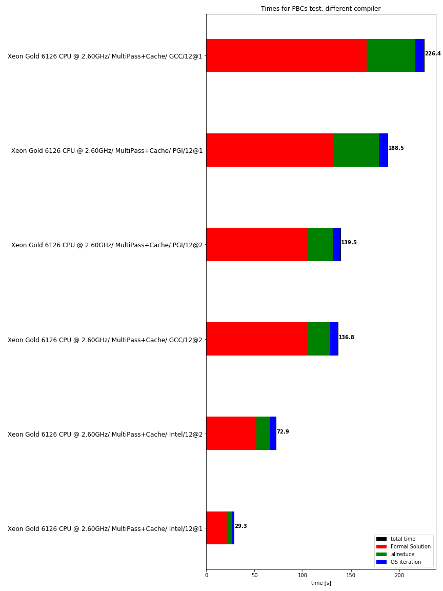
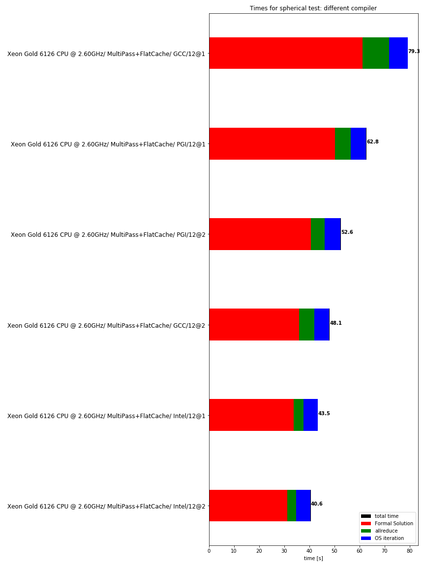
Figure 7: Timing for different compilers with the same algorithms for the Xeon W-3223 system. The horizontal bars give the overall execution walltimes (summed over all iterations) of the different phases of the 3D radiative transfer solver as indicated by the colors. ‘Formal Solution’ designates the phase where new mean intensities are computed from the current estimate of the source function (including the construction of the ${\Lambda^{*}}$ operator in the first iteration), ‘allreduce’ is the phase where the contribution of all MPI processes are collected and summed up via MPI functions and ‘OS iteration’ is the time spent computing the new estimate of the source function (including the solution of the large sparse linear system). The labels on the right hand of the bars give the overall execution time. The labels on the left hand side specify the system or CPU, the algorithm, the solver of the large linear system in the OS step (Jacobi, Gauss-Seidel oder BiCGStab), the compiler and the parallelization setup (where the notation $x$@$y$ indices $x$ MPI processes with $y$ OpenMP thread each).

The timing results for the same jobs on the Xeon W-3223 CPU (this is a MacPro7,1 running MacOS, and when the PGI compiler is used, the NVIDIA HPC SDK is not available for MacOS) different compilers are shown in Fig. 7. For both test setups we used the MultiPass+Cache algorithm with MPI+OpenMP (8 processes with 2 threads each, i.e., hyperthreaded mode) on the system, the fastest results for each compiler are shown in Fig. 7. The compilers are Intel Version 19.1.3.301, GNU Fortran (GCC) 10.2.0, and PGI pgfortran 19.10-0. In both model setups, the Intel compiler results in the smallest run time, followed by GCC which is about 12% slower in the SP test and 42% slower in the PBC test compared to the Intel compiler results. The PGI compiler trails in both tests significantly, a test with the newer NVIDIA HPC compiler on the KNL and the Xeon Silver 4110 (host CPU of the V100 GPU) shows similar trends.

5 Summary and conclusions

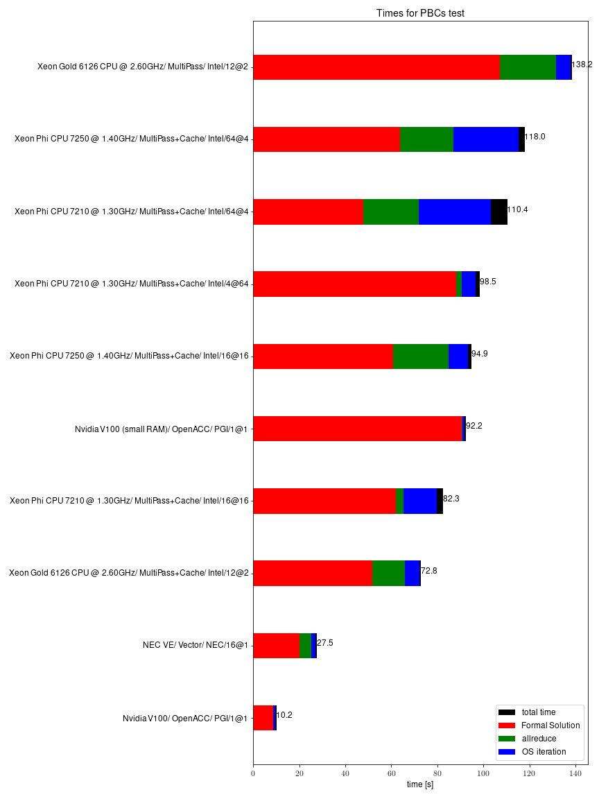
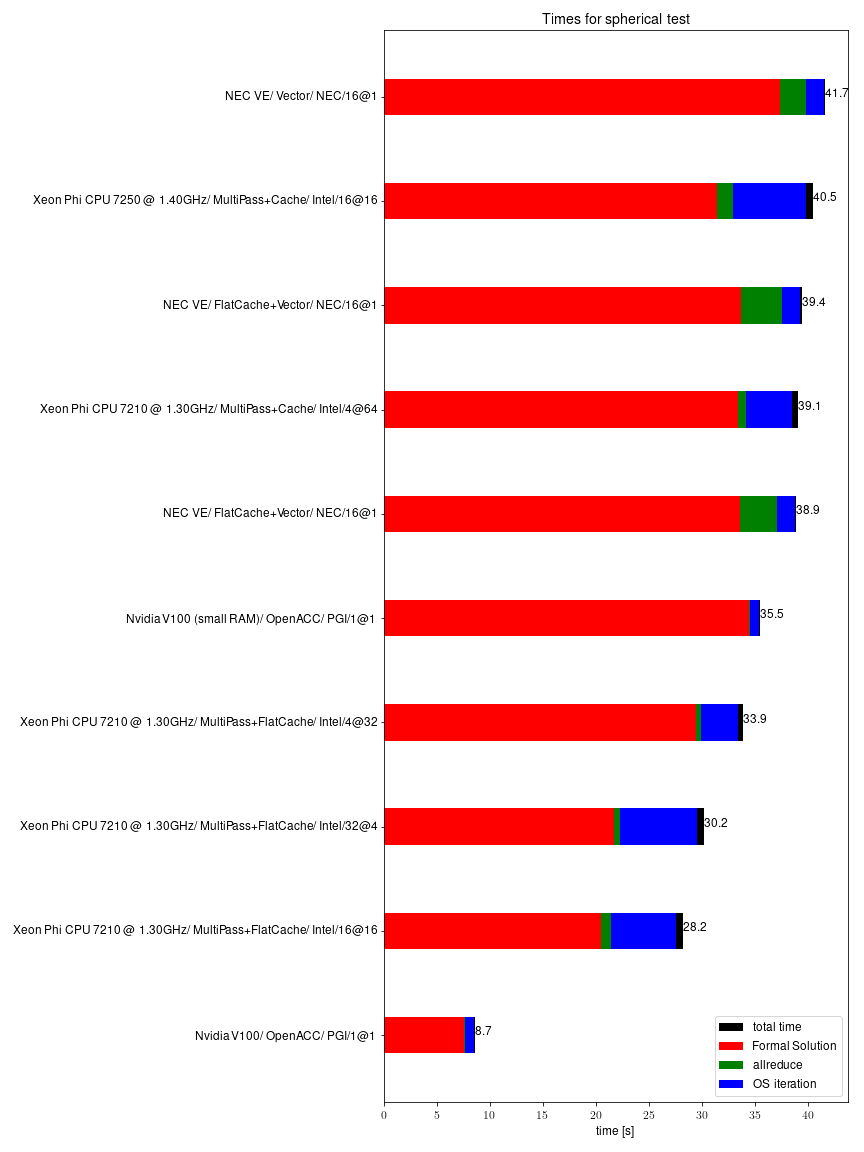
Figure 8: Timing of different algorithms for all considered systems. The horizontal bars give the overall execution walltimes (summed over all iterations) of the different phases of the 3D radiative transfer solver as indicated by the colors. ‘Formal Solution’ designates the phase where new mean intensities are computed from the current estimate of the source function (including the construction of the ${\Lambda^{*}}$ operator in the first iteration), ‘allreduce’ is the phase where the contribution of all MPI processes are collected and summed up via MPI functions and ‘OS iteration’ is the time spent computing the new estimate of the source function (including the solution of the large sparse linear system). The labels on the right hand of the bars give the overall execution time. The labels on the left hand side specify the system or CPU, the algorithm, the solver of the large linear system in the OS step (Jacobi, Gauss-Seidel oder BiCGStab), the compiler and the parallelization setup (where the notation $x$@$y$ indices $x$ MPI processes with $y$ OpenMP thread each). .

In Fig. 8 we show the results for the fastest 7 runs over all systems, algorithms, and setups combined. For the PBC test case, the OpenACC LargeGPU version on the V100 GPU is by far the fastest, followed by the NEC TSUBASA Aurora vector processor which is slower by a factor of about 3.2. In the spherical test case the OpenACC LargeGPU setup is also the fastest, followed by the NEC TSUBASA Aurora which is a factor of about 2.4 slower. The 5 year old KNL is surprisingly quick, it beats the V100 in SmallGPU mode for the PBC tests and is faster than the newer multi-core Xeons. In all cases, the geometry caching is very effective, producing significant speedups, particularly, on more recent CPUs (for example, a Skylake Xeon Gold 6126 is 1.89 faster with the cache enabled than without it). The OpenACC SmallGPU version is much slower than the LargeGPU setup, showing the cost of data transfer. This is of great practical importance as large scale 3DRT runs require more RAM than current GPUs have available, in which case either SmallGPU mode or multiple GPUs must be used. In SmallGPU mode, the overall utilization of the GPU is smaller (by about 50%) so that multiple parallel processes on a single GPU may be used, initial experiments have provided promising results for very large test cases and 2 independent processes on a single V100 GPU (using NVIDIA MPS).

The main problems with OpenACC are that the compiler support needed for efficient and portable (to different GPU vendors) code is not yet available and that complex code and data structures may need to be adapted (simplified) for efficient OpenACC data transfer. Overall, OpenACC code is simple to generate using the vector algorithm as a starting point. In the future it may be better to switch to the OpenMP offload/target paradigm which appears to be available for more hardware options and is supported by more compilers, in particular the LLVM framework.

The NEC Aurora vector processor is very fast and easy to code for, however, its scalar performance is very low. In practical applications it may be best to combine the vector engine with the host CPU whenever possible, where the 3DRT executes on the vector processor and the host CPU is used for I/O and scalar processing. Several methods allow for this option, including running MPI processes on the vector processor and the host CPU at the same time and offloading to and from the vector processor.

The performance of the Xeon Phi KNL is quite sensitive to the exact setup (MPI and OpenMP) used for each problem, thus, in typical production use it is important to determine the optimal configuration beforehand (or to implement an automatic scheme to optimize the configuration at runtime). On all Intel CPUs, the vector algorithm is less efficient than the MultiPass+Cache version (recall that the vector version is a rearranged MultiPass version and includes the geometry cache). This could be due to the Intel compiler not using the vector instructions (which is forced by OpenMP SIMD directives in the MultiPass algorithm) automatically or by the vector instructions stalling to data gather or scatter (which may be hidden by the many threads used on the Xeon Phi).

Our results enable much larger model calculations than were previously feasible. On standard CPU hardware the algorithms developed for the KNL give at least a factor of 3–4 speedup over standard Xeons, if NEC vector or GPU hardware is available speedup factors of 7-21 are possible. As the 3DRT takes 75% of the total simulation time, this speedup can reduce the overall runtime by up to 75%, a massive savings in computer time. Simulations that took a year before, will now take a mere quarter year and/or can be run on much smaller systems. Supercomputers with the required hardware are already available, for example, Summit, or will become available soon, e.g., NERSC’s next generation Perlmutter system.

Future work will include several instances of solar-type stars with chromospheres so that we can define a 3D model of the quiet sun, pre-CV stars in 3D, core collapse and thermonuclear supernovae interacting with their environment, and models of neutron star mergers.

Acknowledgments

PHH gratefully acknowledges support by the DFG under grants HA 3457/20-1 and HA 3457/23-1. Some of the calculations presented here were performed at the RRZ of the Universität Hamburg, at the Höchstleistungs Rechenzentrum Nord (HLRN), and at the National Energy Research Supercomputer Center (NERSC), which is supported by the Office of Science of the U.S. Department of Energy under Contract No. DE-AC03-76SF00098. We thank all these institutions for a generous allocation of computer time. PHH gratefully acknowledges the support of NVIDIA Corporation with the donation of a Quadro P6000 GPU used in this research. E.B. acknowledges support from NASA Grant NNX17AG24G and an AUFF sabbatical grant. We thank Dr. Rudolf Fischer from NEC Deutschland GmbH for very helpful advise on vectorizing for the NEC TSUBASA Aurora system.

Listing 1: Pseudocode for KNL OpenMP Implementation

⬇

!$omp parallel do default(none) collapse(2)

!$omp& private(various_variables)

!$omp& firstprivate(various_variables)

!$omp& shared(various_variables)

!

do iz=-nz,nz ! phase 3 loop:

do iy=-ny,ny

!

!$omp simd

do ix=-nx,nx

!–

!– 0. step: the number of slots used is saved

!–

lngth = chars_pv(ix,iy,iz)

!–

!– 1. step: gather the previous and next points

!– and the path lngths into vectors

!–

i_loop: do i=1,lngth

!–

!– 2. step: gather the previous and next Source and Opacities

!– 3. step: compute dtau, dtau1

!– 4. step: compute alpha, beta, gamma

!– 4a. Fix up for BCs and vacuum

!– 4b. store data for next phase if do_lstar is set

!– 5. step: compute Delta I and exp(dtau)

!–

enddo i_loop

enddo

enddo

enddo ! phase 3 loop

!$omp end parallel do

Listing 2: Pseudocode for OpenACC Implementation

⬇

!–

!– transfer data to the accelerator

!–

!$acc enter data

!$acc& create(various_variables)

!$acc update device(various_variables)

!

!$acc parallel loop collapse(3)

!$acc& present(various_variables)

!

do iz=-nz,nz ! phase 3 loop:

do iy=-ny,ny

do ix=-nx,nx

!–

!– 0. step: the number of slots used is saved

!–

!–

!– 1. step: gather the previous and next points

!– and the path lngths into vectors

!–

!$acc loop seq

i_loop: do i=1,lngth

!–

!– 2. step: gather the previous and next Source and Opacities

!– 3. step: compute dtau, dtau1

!– 4. step: compute alpha, beta, gamma

!– 4a. Fix up for BCs and vacuum

!– 4b. store data for next phase if do_lstar is set

!– 5. step: compute Delta I and exp(dtau)

!–

enddo i_loop

enddo

enddo

enddo ! phase 3 loop

!$acc exit data finalize

!$acc& delete(various_variables)

References

- [1] P. H. Hauschildt, E. Baron, A 3D radiative transfer framework. I. Non-local operator splitting and continuum scattering problems, A&A451 (2006) 273–284. arXiv:astro-ph/0601183, doi:10.1051/0004-6361:20053846.
- [2] E. Baron, P. H. Hauschildt, A 3D radiative transfer framework. II. Line transfer problems, A&A468 (1) (2007) 255–261. doi:10.1051/0004-6361:20066755.
- [3] P. H. Hauschildt, E. Baron, A 3D radiative transfer framework. III. Periodic boundary conditions, A&A490 (2008) 873–877. arXiv:0808.0601, doi:10.1051/0004-6361:200810239.
- [4] P. H. Hauschildt, E. Baron, A 3D radiative transfer framework. IV. Spherical and cylindrical coordinate systems, A&A498 (2009) 981–985. arXiv:0903.1949, doi:10.1051/0004-6361/200911661.
- [5] E. Baron, P. H. Hauschildt, B. Chen, A 3D radiative transfer framework. V. Homologous flows, A&A498 (2009) 987–992. arXiv:0903.2486, doi:10.1051/0004-6361/200911681.
- [6] P. H. Hauschildt, E. Baron, A 3D radiative transfer framework. VI. PHOENIX/3D example applications, A&A509 (2010) A36+. arXiv:0911.3285, doi:10.1051/0004-6361/200913064.
- [7] A. M. Seelmann, P. H. Hauschildt, E. Baron, A 3D radiative transfer framework . VII. Arbitrary velocity fields in the Eulerian frame, A&A522 (2010) A102+. arXiv:1007.3419, doi:10.1051/0004-6361/201014278.
- [8] P. H. Hauschildt, E. Baron, A 3D radiative transfer framework. VIII. OpenCL implementation, A&A533 (2011) A127+. doi:10.1051/0004-6361/201117051.
- [9] D. Jack, P. H. Hauschildt, E. Baron, A 3D radiative transfer framework. IX. Time dependence, A&A546 (2012) A39. arXiv:1209.5788, doi:10.1051/0004-6361/201118152.
- [10] E. Baron, P. H. Hauschildt, B. Chen, S. Knop, A 3D radiative transfer framework. X. Arbitrary velocity fields in the comoving frame, A&A548 (2012) A67. arXiv:1210.6679, doi:10.1051/0004-6361/201219343.
- [11] P. H. Hauschildt, E. Baron, A 3D radiative transfer framework. XI. Multi-level NLTE, A&A566 (2014) A89. arXiv:1404.4376, doi:10.1051/0004-6361/201423574.
- [12] ”Fortran Working Group”, Fortran 2008 Standard, https://wg5-fortran.org/f2008.html (2019).
- [13] ”MPI Working Group”, The MPI Application Programming Interface, https://www.mpi-forum.org/docs/ (2019).
- [14] ”OpenMP Working Group”, The OpenMP Application Programming Interface, https://www.openmp.org/specifications/ (2019).
- [15] ”OpenACC Working Group”, The OpenACC Application Programming Interface, https://www.openacc.org/specification (2019).
- [16] P. H. Hauschildt, H. Störzer, E. Baron, Convergence properties of the accelerated -iteration method for the solution of radaitive transfer problems., J. Quant. Spec. Radiat. Transf.51 (6) (1994) 875–891. doi:10.1016/0022-4073(94)90018-3.
- [17] D. Mihalas, P. B. Kunasz, D. G. Hummer, Solution of the comoving-frame equation of transfer in spherically symmetric flows. I. Computational method for equivalent-two-level-atom source functions., ApJ202 (1975) 465–489. doi:10.1086/153996.
- [18] D. Mihalas, Solution of the comoving-frame equation of transfer in spherically symmetric flows. VI - Relativistic flows, ApJ237 (1980) 574–589. doi:10.1086/157902.
- [19] C. J. Cannon, Angular quadrature perturbations in radiative transfer theory., J. Quant. Spec. Radiat. Transf.13 (7) (1973) 627–633. doi:10.1016/0022-4073(73)90021-6.
- [20] W.-R. Hamann, Line formation in expanding atmospheres: Multi-level calculations using approximate lambda operators, in: W. Kalkofen (Ed.), Numerical Radiative Transfer, Cambridge University Press, 1987, p. 35.
- [21] Richard Barrett, Michael Berry, Tony F. Chan, James Demmel, June Donato, Jack Dongarra, Victor Eijkhout, Roldan Pozo, Charles Romine, Henk van der Vorst, Templates for the Solution of Linear Systems: Building Blocks for Iterative Methods, SIAM, Philadelphia, 1994, iSBN: 978-0-89871-328-2. doi:https://doi.org/10.1137/1.9781611971538.
- [22] NVIDIA, Nvidia cuda: Compute unified device architecture, Tech. rep., NVIDIA Corp (2007).
- [23] A. Munshi, The opencl specification, Tech. rep., Khronos Group, http://www.khronos.org/registry/cl/specs/opencl-1.0.29.pdf (2009).
- [24] NVIDIA, NVIDIA HPC SDK, https://developer.nvidia.com/hpc-sdk (2020).
- [25] ”GNU Project”, GNU Compiler Suite Manuals, https://gcc.gnu.org/onlinedocs/ (2019).