Implications for First-Order Cosmological Phase Transitions from the Third LIGO-Virgo Observing Run

Abstract

We place constraints on the normalized energy density in gravitational waves from first-order strong phase transitions using data from Advanced LIGO and Virgo’s first, second and third observing runs. First, adopting a broken power law model, we place $95\%$ confidence level upper limits simultaneously on the gravitational-wave energy density at 25 Hz from unresolved compact binary mergers, $\Omega_{\rm CBC}<6.1\times 10^{-9}$ , and strong first-order phase transitions, $\Omega_{\rm BPL}<4.4\times 10^{-9}$. The inclusion of the former is necessary since we expect this astrophysical signal to be the foreground of any detected spectrum. We then consider two more complex phenomenological models, limiting at 25 Hz the gravitational-wave background due to bubble collisions to $\Omega_{\rm pt}<5.0\times 10^{-9}$ and the background due to sound waves to $\Omega_{\rm pt}<5.8\times 10^{-9}$ at $95\%$ confidence level for phase transitions occurring at temperatures above $10^{8}$ GeV.

DOI: 10.1103/PhysRevLett.126.151301

Introduction.— The Advanced LIGO Aasi et al. (2015) and Advanced Virgo Acernese et al. (2015) detection of gravitational waves (GWs) from compact binary coalescences (CBCs) Abbott et al. (2020a) offers a novel and powerful tool in understanding our universe and its evolution. We have detected CBCs, and before the detectors reach their designed sensitivity we may detect a stochastic gravitational-wave background (SGWB) produced by many weak, independent and unresolved sources of cosmological or astrophysical origin Allen (1996); Maggiore (2001); Caprini and Figueroa (2018). Among the former, phase transitions occurring in the early universe, is one of the plausible mechanisms leading to a SGWB.

The universe might have undergone a series of phase transitions (see, e.g., Refs. Mazumdar and White (2019); Hindmarsh et al. (2020)). In the case of a first-order phase transition (FOPT), once the temperature drops below a critical value, the universe transitions from a meta-stable phase to a stable one, through a sequence of bubble nucleation, growth, and merger. During this process, a SGWB is expected to be generated Witten (1984); Hogan (1986).

Many compelling extensions of the standard model predict strong FOPTs, e.g., grand unification models Croon et al. (2019); Okada et al. (2020); Huang et al. (2020a), supersymmetric models Huber et al. (2016); Garcia-Pepin and Quiros (2016); Bian et al. (2018); Demidov et al. (2018); Haba and Yamada (2020); Craig et al. (2020), extra dimensions Yu et al. (2019); Megias et al. (2020), composite Higgs models Davoudiasl et al. (2017); Bruggisser et al. (2018); Bian et al. (2019a); De Curtis et al. (2019); Xie et al. (2020); Agashe et al. (2020); Huang et al. (2020b) and models with an extended Higgs sector (see, e.g., Refs. Huang et al. (2016); Ramsey-Musolf (2020)). Generally there might exist symmetries beyond the ones of the standard model, which are spontaneously broken through a FOPT; for example the Peccei-Quinn symmetry Hebecker et al. (2016); Dev et al. (2019); Von Harling et al. (2020); Delle Rose et al. (2020); Ghoshal and Salvio (2020), the $B-L$ symmetry Jinno and Takimoto (2017a); Hasegawa et al. (2019); Bian et al. (2019b); Chao et al. (2017), or the left-right symmetry Brdar et al. (2019). The nature of cosmological phase transitions depends strongly on the particle physics model at high energy scales.

The SGWB sourced by a FOPT spans a wide frequency range. The peak frequency is mainly determined by the temperature $T_{\rm pt}$ at which the FOPT occurs. Interestingly, if $T_{\rm pt}\sim(10^{7}-10^{10})$ GeV – an energy scale not accessible by any existing terrestrial accelerators – the produced SGWB is within the frequency range of Advanced LIGO and Advanced Virgo Lopez and Freese (2015); Dev and Mazumdar (2016). Such an energy scale is well-supported by either the Peccei-Quinn axion model Peccei and Quinn (1977), which solves the strong CP problem and provides a dark matter candidate, or high-scale supersymmetry models Wells (2003); Arvanitaki et al. (2013); Arkani-Hamed et al. (2012), among others. Especially, for axionlike particles, the upper end of the $T_{\rm pt}$ we probe is at the energy scale where astrophysical constraints, such as stellar cooling, lose their sensitivities Hewett:2012ns . In addition, the lower end of the $T_{\rm pt}$ fits well in minisplit SUSY models where the Higgs mass is explained.

The well-motivated SGWB search is performed by cross-correlating strain data from different GW detectors Allen (1996); Romano:2016dpx . No SGWB signal has been observed in the last three observation periods (O1-O3) of the LIGO/Virgo/KAGRA Collaboration (LVKC) Abbott et al. (2020b). Nevertheless, one can use the data to constrain the energy density of gravitational waves, and consequently the underlying particle physics models. This is the aim of this Letter.

SGWB from phase transitions.— In a FOPT, it is well established that GW can be produced by mainly three sources: bubble collisions, sound waves, and magnetohydrodynamic turbulence (see, e.g., Refs. Caprini et al. (2016); Cai et al. (2017); Weir (2018); Hindmarsh et al. (2020) for recent reviews). The GWs thus produced is a SGWB, described by the energy density spectrum: $\Omega_{\rm GW}(f)={d\rho_{\rm GW}}/(\rho_{\rm c}{d\ln f})$ with $\rho_{c}$ the present critical energy density $\rho_{\rm c}=3c^{2}H_{0}^{2}/(8\pi G)$. Each spectrum can be well approximated by a broken power law, with its peak frequency determined by the typical length scale at the transition, the mean bubble separation $R_{\text{pt}}$ which is related to the inverse time duration of the transition $\beta$, and also by the amount of redshifting determined by $T_{\text{pt}}$ and the cosmic history. The amplitude of each contribution is largely determined by the energy released normalized by the radiation energy density $\alpha$, its fraction going into the corresponding source and the bubble wall velocity $v_{\rm w}$. Here we do not consider the contribution from magnetohydrodynamic turbulence as it always happens together with sound waves and is subdominant. In addition, we note that its spectrum is the least understood and might witness significant changes in the future Caprini et al. (2016); Kahniashvili et al. (2008a, b); Kahniashvili et al. (2010); Caprini et al. (2009); Kisslinger and Kahniashvili (2015); Roper Pol et al. (2019).

The dominant source for GW production in a thermal transition, as most commonly encountered in the early universe, is the sound waves in the plasma induced by the coupling between the scalar field and the thermal bath Hindmarsh et al. (2015, 2014, 2017). A good analytical understanding of this spectrum has been achieved through the sound shell model Hindmarsh (2018); Hindmarsh and Hijazi (2019); Guo et al. (2021), though it still does not capture all the physics Hindmarsh et al. (2017); Cutting et al. (2020a); Hindmarsh et al. (2020) to match perfectly the result from numerical simulations Caprini et al. (2016); Hindmarsh et al. (2015). We use the spectrum from numerical simulations:

$$\Omega_{\textrm{sw}}(f)h^{2}=2.65\times 10^{-6}\left(\frac{H_{\rm pt}}{\beta}\right)\left(\frac{\kappa_{\rm sw}\alpha}{1+\alpha}\right)^{2}\left(\frac{100}{g_{\ast}}\right)^{1/3}$$

$$\times v_{\rm w}\left(\frac{f}{f_{\text{sw}}}\right)^{3}\left(\frac{7}{4+3(f/f_{\textrm{sw}})^{2}}\right)^{7/2}\Upsilon(\tau_{\text{sw}})\ ,\quad$$ (1)

where $\kappa_{\rm sw}$ is the fraction of vacuum energy converted into the kinetic energy of the bulk flow, a function of $v_{\rm w}$ and $\alpha$ Espinosa et al. (2010); Giese et al. (2020); $H_{\rm pt}$ is the Hubble parameter at $T_{\text{pt}}$; $g_{\ast}$ is the number of relativistic degrees of freedom, chosen to be 100 in our analysis; $h$ is the dimensionless Hubble parameter; $f_{\textrm{sw}}$ is the present peak frequency,

$$f_{\textrm{sw}}=19\frac{1}{v_{\rm w}}\left(\frac{\beta}{H_{\rm pt}}\right)\left(\frac{T_{\rm pt}}{100\textrm{GeV}}\right)\left(\frac{g_{\ast}}{100}\right)^{\frac{1}{6}}\mu\textrm{Hz},$$ (2)

and $\Upsilon=1-(1+2\tau_{\text{sw}}H_{\rm pt})^{-1/2}$ Guo et al. (2021) which is a suppression factor due to the finite lifetime Guo et al. (2021); Ellis et al. (2020), $\tau_{\text{sw}}$, of sound waves. $\tau_{\text{sw}}$ is typically smaller than a Hubble time unit Ellis et al. (2019a); Caprini et al. (2020) and is usually chosen to be the timescale for the onset of turbulence Weir (2018), $\tau_{\text{sw}}\approx{R_{\rm pt}}/{\bar{U}_{f}}$, with $R_{\rm pt}=(8\pi)^{1/3}v_{\rm w}/\beta$ for an exponential nucleation of bubbles Hindmarsh and Hijazi (2019); Guo et al. (2021), and $\bar{U}_{f}^{2}=3\kappa_{\rm sw}\alpha/[4(1+\alpha)]$ Weir (2018).

When sound waves, and thus also magnetohydrodynamic turbulence, are highly suppressed or absent, bubble collisions can become dominant, e.g., for a FOPT in vacuum of a dark sector which has no or very weak interactions with the standard plasma. The resulting GW spectrum can be well modeled with the envelope approximation Kosowsky and Turner (1993); Kosowsky et al. (1992); Jinno and Takimoto (2017b), which assumes an infinitely thin bubble wall and neglects the contribution from overlapping bubble segments. In the low-frequency regime, $\Omega_{\rm GW}\propto f^{3}$ from causality Maggiore (2018), and for high-frequencies $\Omega_{\rm GW}\propto f^{-1}$ Huber and Konstandin (2008) due to the dominant single bubble contribution as revealed by the analytical calculation Jinno and Takimoto (2017b). The spectrum is Huber and Konstandin (2008); Jinno and Takimoto (2017b); Weir (2018)

$$\Omega_{\rm coll}(f)h^{2}=1.67\times 10^{-5}\Delta\left({H_{\rm pt}\over\beta}\right)^{2}\left({\kappa_{\phi}\alpha\over 1+\alpha}\right)^{2}$$

$$\times\left({100\over g_{\ast}}\right)^{1/3}S_{\text{env}}(f),$$ (3)

where $\kappa_{\phi}=\rho_{\phi}/\rho_{\rm vac}$ denotes the fraction of vacuum energy converted into gradient energy of the scalar field. The amplitude $\Delta$ is $\Delta(v_{\rm w})=0.48v_{\rm w}^{3}/(1+5.3v_{\rm w}^{2}+5v_{\rm w}^{4})$ and the spectral shape is $S_{\text{env}}=1/(c_{l}\tilde{f}^{-3}+(1-c_{l}-c_{h})\tilde{f}^{-1}+c_{h}\tilde{f})$ where $c_{l}=0.064$, $c_{h}=0.48$ and $\tilde{f}=f/f_{\text{env}}$ with $f_{\text{env}}$ the present peak frequency

$$f_{\text{env}}=16.5\left(\frac{f_{\rm bc}}{\beta}\right)\left(\frac{\beta}{H_{\rm pt}}\right)\left(\frac{T_{\rm pt}}{100\ \text{GeV}}\right)\left(\frac{g_{\ast}}{100}\right)^{\frac{1}{6}}\mu\text{Hz},$$ (4)

and $f_{\rm bc}$ the peak frequency right after the transition ${f_{\rm bc}}={0.35\beta}/(1+0.069v_{\rm w}+0.69v_{\rm w}^{4})$. More recent simulations going beyond the envelope approximation show a steeper shape $f^{-1.5}$ for high frequencies Cutting et al. (2018), and it also varies from $f^{-1.4}$ to $f^{-2.3}$ as the wall thickness increases Cutting et al. (2020b) (see also Refs. Lewicki and Vaskonen (2020a, b); Di et al. (2020)).

Data Analysis.— Here we take two analysis approaches. First, we consider an approximated broken power law including main features of the shape and its peak. We then consider the phenomenological models Eqs. (3) and (1), for contributions from bubble collisions and sound waves.

I. Broken power law model: The spectrum can be approximated by a broken power law (BPL) as

$$\Omega_{\rm bpl}(f)=\Omega_{*}~{}\Big{(}\frac{f}{f_{*}}\Big{)}^{n_{1}}~{}\Bigg{[}1+\Big{(}\frac{f}{f_{*}}\Big{)}^{\Delta}\Bigg{]}^{(n_{2}-n_{1})/\Delta}.$$ (5)

Here $n_{1}=3$, from causality, and $n_{2}$ takes the values $-4$ and $-1$, for sound waves and bubble collisions, respectively. We fix the $n_{1}$ parameter in our search, but we let $n_{2}$ vary uniformly between -8 and 0, allowing for the values motivated by both contributions. The value for $\Delta$ is set to 2 for sound waves and 4 for approximating bubble collisions. We run a Bayesian search for both values, but present results only for $\Delta=2$, since it gives more conservative upper limits.

We follow Refs. Mandic et al. (2012); Callister et al. (2017); Meyers et al. (2020) to perform a Bayesian search and model selection. In addition to a search for the broken power law, we undertake a study on simultaneous estimation of a CBC background and a broken power law background, because current estimates of the CBC background Abbott et al. (2018, 2020b) show it as a non-negligible component of any SGWB signal. The CBC background is very well approximated by an $f^{2/3}$ power law Callister et al. (2016). The challenge then is to search for a broken power law in the presence of a CBC background.

The log-likelihood for a single detector pair is Gaussian,

$$\log p(\hat{C}_{IJ}(f)|\bm{\theta}_{\rm gw},\lambda)\propto-\frac{1}{2}\sum_{f}\frac{\left[\hat{C}_{IJ}(f)-\lambda\,\Omega_{\rm gw}(f,\bm{\theta}_{\rm gw})\right]^{2}}{\sigma_{IJ}^{2}(f)},$$ (6)

where $\hat{C}_{IJ}(f)$ and $\sigma_{IJ}(f)$ are data products of the analysis: $\hat{C}_{IJ}(f)$ is the cross-correlation estimator of the SGWB calculated using data from detectors $I$ and $J$, and $\sigma^{2}_{IJ}(f)$ is its variance Allen and Romano (1999). The search for an isotropic stochastic signal shows no evidence of correlated magnetic noise, and a pure Gaussian noise model is still preferred by the data Abbott et al. (2020b). Therefore, here, a contribution from Schumann resonances E. Thrane, N. Christensen and R. Schofield ; M. W. Coughlin, A. Cirone, P. Meyers, S. Atsuta, V. Boschi, A. Chincarini, N. L. Christensen, R. De Rosa, A. Effler and I. Fiori, et al. ; Meyers et al. (2020) is neglected. The model we fit to the data is $\Omega_{\rm GW}(f,\bm{\theta}_{\rm GW})$, with parameters $\bm{\theta}_{\rm GW}$. The parameter $\lambda$ captures calibration uncertainties of the detectors Sun et al. (2020) and is marginalized over Whelan et al. (2014). For a multibaseline study, we add all log-likelihoods of individual baselines. The set of GW parameters depends on the type of search we perform.

The CBC spectrum is modeled as

$$\Omega_{\rm cbc}=\Omega_{\rm ref}(f/f_{\rm ref})^{2/3},$$ (7)

with $f_{\rm ref}=25~{}\rm{Hz}$. We consider three separate scenarios: contributions from unresolved CBC sources, with $\bm{\theta}_{\rm GW}=(\Omega_{\rm ref})$; broken power law contributions, with $\bm{\theta}_{\rm GW}=({\Omega_{*},f_{*},n_{2}})$; and the combination of CBC and broken power law contributions, for which $\bm{\theta}_{\rm GW}=({\Omega_{\rm ref},\Omega_{*},f_{*},n_{2}})$. The priors used are summarized in Table 1. To compare GW models and assess which provides a better fit, we use ratios of evidences, otherwise known as Bayes factors. In particular, we consider $\log\cal{B}^{\rm CBC+BPL}_{\rm noise}$ and $\log\cal{B}^{\rm CBC+BPL}_{\rm CBC}$ as indicative detection statistics.

Broken power law model
Parameter	Prior
$\Omega_{\rm ref}$	LogUniform($10^{-10}$, $10^{-7}$)
$\Omega_{*}$	LogUniform($10^{-9}$, $10^{-4}$)
$f_{*}$	Uniform(0, 256 Hz)
$n_{1}$	3
$n_{2}$	Uniform(-8,0)
$\Delta$	2
Phenomenological model
Parameter	Prior
$\Omega_{\rm ref}$	LogUniform($10^{-10}$, $10^{-7}$)
$\alpha$	LogUniform ($10^{-3}$, $10$)
$\beta/H_{\rm pt}$	LogUniform ($10^{-1}$, $10^{3}$)
$T_{\rm pt}$	LogUniform ($10^{5}$, $10^{10}$ GeV)
$v_{\rm w}$	1
$\kappa_{\phi}$	1
$\kappa_{\rm sw}$	$f(\alpha,v_{\rm w})\in[0.1-0.9]$

Table 1: List of prior distributions used for all parameters in the various searches. The narrow, informative prior on $\Omega_{\rm ref}$ stems from estimates of the CBC background Abbott et al. (2018), and encompasses uncertainties on the mass and redshift distributions of CBCs Abbott et al. (2020b, 2016). The frequency prior is uniform across the frequency range considered since we have no further information about it.

II. Phenomenological model: Two scenarios are considered, corresponding to dominant contributions from bubble collisions or sound waves, respectively, following an approach similar to Ref. Von Harling et al. (2020). The analysis procedure follows closely that of the broken power law search, with $\bm{\theta}_{\rm GW}=({\Omega_{\rm ref},\alpha,\beta/H_{\rm pt},T_{\rm pt}})$ including CBC background $\Omega_{\rm CBC}$, and $\Omega_{\rm GW}$ from bubble collisions and sound waves described by Eqs. (3) and  (1), respectively.

For bubble collisions, $v_{\rm w}$ and $\kappa_{\phi}$ are set to unity. The remaining model parameters are varied in the ranges in Table 1. We note that the GW spectra in Eqs. (3) and  (1) may not be applicable when $\alpha\gtrsim 10$, and also a large $\alpha$ does not translate into a significant increase in the GW amplitude. Moreover, $\beta/H_{\text{pt}}$ is related to the mean bubble separation, up to an $O(1)$ coefficient, and one should be cautious when it is smaller than $1$ Ellis et al. (2019b, a). In this study, we conservatively choose $\beta/H_{\text{pt}}$ to be larger than 0.1.

For sound waves, we initially set $v_{\rm w}=1$, and then explore different values for $v_{\rm w}$ in the range (0.7 - 1.0), corresponding to various detonation and hybrid modes of fluid velocity profile Cutting et al. (2020a); Espinosa et al. (2010). Here $\kappa_{\rm sw}$ is a function of $\alpha$ and $v_{\rm w}$, e.g., for $v_{\rm w}=1$, $\kappa_{\rm sw}$ increases from 0.1 to 0.9 as $\alpha$ increases from 0.1 to 10. The rest of the parameters are varied as in the case of bubble collisions.

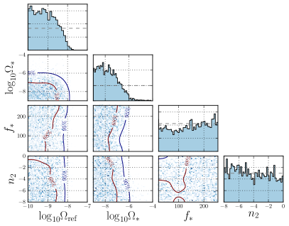
Figure 1: Posterior distributions for the combined CBC and broken power law search as a function of $\log\Omega_{\rm ref}$ and the different parameters of the model. The 68$\%$ and $95\%$ CL exclusion contours are shown. The horizontal dashed line in the posteriors indicate the flat priors used in the analysis.

Results.— I. Broken power law model: In Fig. 1 we present posterior distributions of parameters in the combined CBC and BPL search. The Bayes factor is $\log{\cal{B}}^{\rm CBC+BPL}_{\rm noise}=-1.4$, demonstrating no evidence of such a signal in the data from the three observing runs. The 2-d posterior of $\Omega_{\rm ref}$ and $\Omega_{*}$ allows us to place simultaneous estimates on the amplitudes of the two spectra. The 95% confidence level (CL) upper limits are $\Omega_{\rm ref}=6.1\times 10^{-9}$ and $\Omega_{*}=5.6\times 10^{-7}$, respectively. If we take individual posterior samples of $\Omega_{*}$, $f_{*}$ and $n_{2}$ from Fig. 1, and combine them to construct a posterior of $\Omega_{\rm BPL}$, we estimate at 95% CL $\Omega_{\rm BPL}(25\,\rm Hz)=4.4\times 10^{-9}$. The width of the $n_{2}$ posterior suggests no preference for a particular value by the data, and we are unable to rule out any part of the parameter space at this time. Other searches give Bayes factors $\log{\cal{B}}^{\rm BPL}_{\rm noise}=-0.78$ and $\log{\cal{B}}^{\rm CBC+BPL}_{\rm CBC}=-0.81$, once again giving no evidence for a BPL signal, with or without CBCs considered.

To demonstrate the dependence of GW amplitude constraints on other parameters, we present 95% CL upper limits on $\Omega_{*}$ for a set of $n_{2}$ and $f_{*}$ in Table 2. We choose representative values of $n_{2}$, for bubble collisions, $n_{2}=$ -1 and -2, and for sound waves, $n_{2}=$ -4. The $f_{*}$ values are chosen to represent broken power laws that peak before, at, and after the most sensitive part of the LIGO-Virgo band, $f_{*}=\,25\,\rm{Hz}$. As expected, the most constraining upper limits are obtained for a signal that peaks at 25 Hz. For the signal in the first column that peaks at 1 Hz, the faster it decays, the weaker it is at 25 Hz. Therefore, the more negative $n_{2}$ values give less constraining upper limits on the amplitude. Finally, the signal that peaks at 200 Hz gives similar $\Omega_{*}$ upper limits for all values of $n_{2}$ since it resembles a simple $n_{1}=3$ power law in the range with largest SNR. Note the upper limits in Table 2 are fundamentally different from results in Fig. 1. In the former case we fix $f_{*}$ and $n_{2}$ and find $\Omega_{*}^{95\%}$, while in the latter we marginalize over all parameters to obtain $\Omega_{*}^{95\%}$.

Broken power law model
	$f_{*}=1\,\rm{Hz}$	$f_{*}=25\,\rm{Hz}$	$f_{*}=200\,\rm{Hz}$
$n_{2}=-1$	$3.3\times 10^{-7}$	$3.5\times 10^{-8}$	$2.8\times 10^{-7}$
$n_{2}=-2$	$8.2\times 10^{-6}$	$6.0\times 10^{-8}$	$3.7\times 10^{-7}$
$n_{2}=-4$	$5.2\times 10^{-5}$	1.8 $\times 10^{-7}$	$3.7\times 10^{-7}$

Table 2: Upper limits for the energy density amplitude, $\Omega_{*}^{95\%}$, in the broken power law model for fixed values of the peak frequency, $f_{*}$, and negative power law index, $n_{2}$.

II. Phenomenological model: We now estimate 95$\%$ CL upper limits on $\Omega_{\rm coll}$ and $\Omega_{\rm sw}$ from bubble collisions and sound waves respectively. The Bayesian analysis is repeated separately for $\Omega_{\rm coll}$ and $\Omega_{\rm sw}$ contributions, with priors stated in Table 1, leading to Bayes factors $\log\cal{B}^{\rm CBC+coll}_{\rm noise}$= -0.74 and $\log\cal{B}^{\rm CBC+sw}_{\rm noise}$= -0.66, respectively.

In Fig. 2 we present exclusion regions as a function of the different parameters of the CBC+FOPT model, now under the assumption that contributions from bubble collisions dominate, with $v_{\rm w}=1$ and $\kappa_{\phi}=1$. In general, with the chosen prior, the data can exclude part of the parameter space at 95$\%$ CL, especially when $T_{\rm pt}>10^{8}$ GeV, $\alpha>1$, or $\beta/H_{\rm pt}<1$.

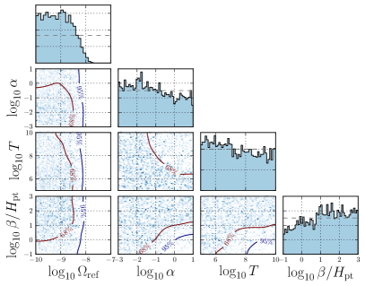
Figure 2: Posterior distributions for the CBC+FOPT search in the case of a phenomenological model with dominant bubble collision contributions as a function of $\log\Omega_{\rm ref}$ and the different parameters of the model. The 68$\%$ and $95\%$ CL exclusion contours are shown. The horizontal dashed line in the posteriors indicate the flat priors used in the analysis.

Table III presents 95$\%$ CL upper limits on $\Omega_{\rm coll}$(25 Hz) for several $\beta/H_{\rm pt}$ and $T_{\rm pt}$, where $\alpha$ is left as a free parameter to be inferred from the data. We consider three values for $\beta/H_{\rm pt}$, namely 0.1, 1, and 10, and four for $T_{\rm pt}$: $10^{7}$, $10^{8}$, $10^{9}$, and $10^{10}$ GeV. Our constraints on $\Omega_{\rm coll}$(25 Hz), as computed at the reference frequency of 25 Hz, vary in the range $4.0\times 10^{-9}$ to $1.0\times 10^{-8}$, with more stringent limits at large $\beta/H_{\rm pt}$ or large $T_{\rm pt}$. At the largest values of $\beta/H_{\rm pt}$ and $T_{\rm pt}$ there is not enough sensitivity to place constrains to the model. In all cases, the inferred upper limits on the CBC background range between $\Omega_{\rm ref}$ = $5.3\times 10^{-9}$ and $6.1\times 10^{-9}$.

Phenomenological model (bubble collisions)
$\Omega_{\rm coll}^{95\%}$ (25 Hz)
$\beta/H_{\rm pt}\setminus T_{\rm pt}$	$10^{7}$ GeV	$10^{8}$ GeV	$10^{9}$ GeV	$10^{10}$ GeV
0.1	$9.2\times 10^{-9}$	$8.8\times 10^{-9}$	$1.0\times 10^{-8}$	$7.2\times 10^{-9}$
1	$1.0\times 10^{-8}$	$8.4\times 10^{-9}$	$5.0\times 10^{-9}$	$-$
10	$4.0\times 10^{-9}$	$6.3\times 10^{-9}$	$-$	$-$

Table 3: The 95$\%$ CL upper limits on $\Omega_{\rm coll}^{95\%}$(25 Hz) for fixed values of $\beta/H_{\rm pt}$ and $T_{\rm pt}$, and $v_{\rm w}=\kappa_{\phi}=1$. The dashed lines denote no sensitivity for exclusion.

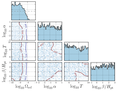
Figure 3: Posterior distributions for the CBC+FOPT search in the case of a phenomenological model with dominant sound wave contributions ($v_{\rm w}=1$), as a function of $\log\Omega_{\rm ref}$ and the different parameters of the model. The 68$\%$ and $95\%$ CL exclusion contours are shown. The horizontal dashed line in the posteriors indicate the flat priors used in the analysis.

Similarly, in Fig. 3 we present the results for the CBC+FOPT hypothesis in which the sound waves dominate with $v_{\rm w}=1$ and $\kappa_{\rm sw}$ a function of $v_{\rm w}$ and $\alpha$. The Bayesian analysis shows sensitivity at large values of $\alpha$ and $T_{\rm pt}$, but does not exclude regions in the parameter space at 95$\%$ CL. The analysis is then performed for given values of $\beta/H_{\rm pt}$ and $T_{\rm pt}$ leaving $\alpha$ as a free parameter. As a result, a 95$\%$ CL upper limit on $\Omega_{\rm sw}$(25 Hz) of $5.9\times 10^{-9}$ is obtained for $\beta/H_{\rm pt}<1$ and $T_{\rm pt}>10^{8}$ GeV. The analysis is repeated for models with reduced velocities of $v_{\rm w}=0.9$, $v_{\rm w}=0.8$, and $v_{\rm w}=0.7$, with Bayes factor $\log{\cal{B}}^{\rm CBC+sw}_{\rm noise}=-0.60$ and upper limit $\Omega_{\rm ref}\approx 5.9\times 10^{-9}$, with no significant $v_{w}$ dependence. In all studied cases, the models with reduced $v_{w}$ lead to significantly lower sound waves predicted energy densities, and with no 95$\%$ CL exclusions.

Conclusions.—We have searched for signals from FOPTs in the early universe, potentially leading to a SGWB in the Advanced LIGO/Advanced Virgo frequency band. The analysis is based on the data from the three observation periods, for which no generic stochastic signals above the detector noise has been observed.

We use the results to deduce implications for models describing SGWB. We first consider a generic broken power law spectrum, describing its main features in terms of the shape and the peak amplitude. We place $95\%$ CL upper limits simultaneously on the normalized energy density contribution from unresolved CBCs and a FOPT, $\Omega_{\rm CBC}(25\,\rm{Hz})=6.1\times 10^{-9}$ and $\Omega_{\rm BPL}(25\,\rm Hz)=4.4\times 10^{-9}$, respectively.

The results are then interpreted in terms of a phenomenological model describing contributions from bubble collisions or sound waves, showing that the data can exclude a part of the parameter space at large temperatures. In a scenario in which bubble collision contributions dominate, with $v_{\rm w}=1$ and $\kappa_{\phi}=1$, part of the phase space with $T_{\rm pt}>10^{8}$ GeV, $\alpha>1$, and $\beta/H_{\rm pt}<1$ is excluded at $95\%$ CL. For fixed values of $\beta/H_{\rm pt}=0.1$, $1$ or $10$ and $T_{\rm pt}=10^{7},10^{8},10^{9}$ or $10^{10}{\rm\ GeV}$, the 95$\%$ CL upper limits on $\Omega_{\rm coll}(25\rm{Hz})$ vary in the range between $4.0\times 10^{-9}$ and $1.0\times 10^{-8}$ which depends on the $\beta/H_{\rm pt}$ and $T_{\rm pt}$ values considered. In the case where sound waves dominate, several scenarios are explored considering different $v_{w}$. The data only shows a limited sensitivity, and a 95$\%$ CL upper limit on $\Omega_{\rm sw}(25{\rm Hz})$ of $5.9\times 10^{-9}$ is placed in the case of $v_{\rm w}=1$, for $\beta/H_{\rm pt}<0.1$ and $T_{\rm pt}>10^{8}$ GeV. Altogether, the results indicate the importance of using LIGO-Virgo GW data to place constraints on new phenomena related to strong FOPTs in the early universe packagesnote .

The authors would like to thank the LIGO-Virgo stochastic background group for helpful comments and discussions. In particular, the authors thank Patrick M. Meyers on his contributions to the parameter estimation analysis code. We thank Alberto Mariotti on his useful feedback on the draft. The authors are grateful for computational resources provided by the LIGO Laboratory and supported by National Science Foundation Grants PHY-0757058 and PHY-0823459. This paper has been given LIGO DCC number LIGO-P2000518.

A.R and M.M would like to thank O. Pujolàs for the motivation and the fruitful discussions. This work was partially supported by the Spanish MINECO under the grants SEV-2016-0588 and PGC2018-101858-B-I00, some of which include ERDF funds from the European Union. IFAE is partially funded by the CERCA program of the Generalitat de Catalunya. K.M. is supported by King’s College London through a Postgraduate International Scholarship. M.S. is supported in part by the Science and Technology Facility Council (STFC), United Kingdom, under the research grant ST/P000258/1. H.G. is supported by the U.S. Department of Energy grant No. DE-SC0009956. F.W.Y. and Y.Z. are supported by the U.S. Department of Energy under Award No. DE-SC0009959.

References

- Aasi et al. (2015) J. Aasi, B. P. Abbott, R. Abbott, T. Abbott, M. R. Abernathy, K. Ackley, C. Adams, T. Adams, P. Addesso, and R. X. A. et. al., Class. Quant. Grav. 32, 074001 (2015), URL https://doi.org/10.1088/0264-9381/32/7/074001.
- Acernese et al. (2015) F. Acernese et al. (Virgo), Class. Quant. Grav. 32, 024001 (2015), eprint 1408.3978.
- Abbott et al. (2020a) R. Abbott et al. (LIGO Scientific, Virgo) (2020a), eprint 2010.14527.
- Allen (1996) B. Allen, in Les Houches School of Physics: Astrophysical Sources of Gravitational Radiation (1996), pp. 373–417, eprint gr-qc/9604033.
- Maggiore (2001) M. Maggiore, ICTP Lect. Notes Ser. 3, 397 (2001), eprint gr-qc/0008027.
- Caprini and Figueroa (2018) C. Caprini and D. G. Figueroa, Class. Quant. Grav. 35, 163001 (2018), eprint 1801.04268.
- Mazumdar and White (2019) A. Mazumdar and G. White, Rept. Prog. Phys. 82, 076901 (2019), eprint 1811.01948.
- Hindmarsh et al. (2020) M. B. Hindmarsh, M. Lüben, J. Lumma, and M. Pauly (2020), eprint 2008.09136.
- Witten (1984) E. Witten, Phys. Rev. D 30, 272 (1984).
- Hogan (1986) C. Hogan, Mon. Not. Roy. Astron. Soc. 218, 629 (1986).
- Croon et al. (2019) D. Croon, T. E. Gonzalo, L. Graf, N. Koˇsnik, and G. White, Front. in Phys. 7, 76 (2019), eprint 1903.04977.
- Okada et al. (2020) N. Okada, O. Seto, and H. Uchida (2020), eprint 2006.01406.
- Huang et al. (2020a) W.-C. Huang, F. Sannino, and Z.-W. Wang (2020a), eprint 2004.02332.
- Huber et al. (2016) S. J. Huber, T. Konstandin, G. Nardini, and I. Rues, JCAP 03, 036 (2016), eprint 1512.06357.
- Garcia-Pepin and Quiros (2016) M. Garcia-Pepin and M. Quiros, JHEP 05, 177 (2016), eprint 1602.01351.
- Bian et al. (2018) L. Bian, H.-K. Guo, and J. Shu, Chin. Phys. C 42, 093106 (2018), [Erratum: Chin.Phys.C 43, 129101 (2019)], eprint 1704.02488.
- Demidov et al. (2018) S. Demidov, D. Gorbunov, and D. Kirpichnikov, Phys. Lett. B 779, 191 (2018), eprint 1712.00087.
- Haba and Yamada (2020) N. Haba and T. Yamada, Phys. Rev. D 101, 075027 (2020), eprint 1911.01292.
- Craig et al. (2020) N. Craig, N. Levi, A. Mariotti, and D. Redigolo (2020), eprint 2011.13949.
- Yu et al. (2019) H. Yu, Z.-C. Lin, and Y.-X. Liu, Commun. Theor. Phys. 71, 991 (2019), eprint 1905.10614.
- Megias et al. (2020) E. Megias, G. Nardini, and M. Quiros (2020), eprint 2005.04127.
- Davoudiasl et al. (2017) H. Davoudiasl, P. P. Giardino, E. T. Neil, and E. Rinaldi, Phys. Rev. D 96, 115003 (2017), eprint 1709.01082.
- Bruggisser et al. (2018) S. Bruggisser, B. Von Harling, O. Matsedonskyi, and G. Servant, JHEP 12, 099 (2018), eprint 1804.07314.
- Bian et al. (2019a) L. Bian, Y. Wu, and K.-P. Xie, JHEP 12, 028 (2019a), eprint 1909.02014.
- De Curtis et al. (2019) S. De Curtis, L. Delle Rose, and G. Panico, JHEP 12, 149 (2019), eprint 1909.07894.
- Xie et al. (2020) K.-P. Xie, Y. Wu, and L. Bian (2020), eprint 2005.13552.
- Agashe et al. (2020) K. Agashe, P. Du, M. Ekhterachian, S. Kumar, and R. Sundrum, JHEP 05, 086 (2020), eprint 1910.06238.
- Huang et al. (2020b) W.-C. Huang, M. Reichert, F. Sannino, and Z.-W. Wang (2020b), eprint 2012.11614.
- Huang et al. (2016) P. Huang, A. J. Long, and L.-T. Wang, Phys. Rev. D94, 075008 (2016), eprint 1608.06619.
- Ramsey-Musolf (2020) M. J. Ramsey-Musolf, JHEP 09, 179 (2020), eprint 1912.07189.
- Hebecker et al. (2016) A. Hebecker, J. Jaeckel, F. Rompineve, and L. T. Witkowski, JCAP 11, 003 (2016), eprint 1606.07812.
- Dev et al. (2019) P. B. Dev, F. Ferrer, Y. Zhang, and Y. Zhang, JCAP 11, 006 (2019), eprint 1905.00891.
- Von Harling et al. (2020) B. Von Harling, A. Pomarol, O. Pujolàs, and F. Rompineve, JHEP 04, 195 (2020), eprint 1912.07587.
- Delle Rose et al. (2020) L. Delle Rose, G. Panico, M. Redi, and A. Tesi, JHEP 04, 025 (2020), eprint 1912.06139.
- Ghoshal and Salvio (2020) A. Ghoshal and A. Salvio (2020), eprint 2007.00005.
- Jinno and Takimoto (2017a) R. Jinno and M. Takimoto, Phys. Rev. D 95, 015020 (2017a), eprint 1604.05035.
- Hasegawa et al. (2019) T. Hasegawa, N. Okada, and O. Seto, Phys. Rev. D 99, 095039 (2019), eprint 1904.03020.
- Bian et al. (2019b) L. Bian, W. Cheng, H.-K. Guo, and Y. Zhang (2019b), eprint 1907.13589.
- Chao et al. (2017) W. Chao, W.-F. Cui, H.-K. Guo, and J. Shu (2017), eprint 1707.09759.
- Brdar et al. (2019) V. Brdar, L. Graf, A. J. Helmboldt, and X.-J. Xu, JCAP 12, 027 (2019), eprint 1909.02018.
- Lopez and Freese (2015) A. Lopez and K. Freese, JCAP 01, 037 (2015), eprint 1305.5855.
- Dev and Mazumdar (2016) P. S. B. Dev and A. Mazumdar, Phys. Rev. D93, 104001 (2016), eprint 1602.04203.
- Peccei and Quinn (1977) R. Peccei and H. R. Quinn, Phys. Rev. D 16, 1791 (1977).
- Wells (2003) J. D. Wells, in 11th International Conference on Supersymmetry and the Unification of Fundamental Interactions (2003), eprint hep-ph/0306127.
- Arvanitaki et al. (2013) A. Arvanitaki, N. Craig, S. Dimopoulos, and G. Villadoro, JHEP 02, 126 (2013), eprint 1210.0555.
- Arkani-Hamed et al. (2012) N. Arkani-Hamed, A. Gupta, D. E. Kaplan, N. Weiner, and T. Zorawski (2012), eprint 1212.6971.
- (47) J. L. Hewett, H. Weerts, R. Brock, J. N. Butler, B. C. K. Casey, J. Collar, A. de Gouvea, R. Essig, Y. Grossman and W. Haxton, et al. doi:10.2172/1042577 [arXiv:1205.2671 [hep-ex]].
- (48) J. D. Romano and N. J. Cornish, Living Rev. Rel. 20, (2017), eprint 1608.06889.
- Abbott et al. (2020b) B. Abbott et al. (LIGO Scientific Collaboration, Virgo Collaboration), LIGO-DCC:P2000314 (2020b), URL https://dcc.ligo.org/LIGO-P2000314/public.
- Caprini et al. (2016) C. Caprini et al., JCAP 1604, 001 (2016), eprint 1512.06239.
- Cai et al. (2017) R.-G. Cai, Z. Cao, Z.-K. Guo, S.-J. Wang, and T. Yang (2017), eprint 1703.00187.
- Weir (2018) D. J. Weir, Phil. Trans. Roy. Soc. Lond. A 376, 20170126 (2018), eprint 1705.01783.
- Kahniashvili et al. (2008a) T. Kahniashvili, A. Kosowsky, G. Gogoberidze, and Y. Maravin, Phys. Rev. D 78, 043003 (2008a), eprint 0806.0293.
- Kahniashvili et al. (2008b) T. Kahniashvili, L. Campanelli, G. Gogoberidze, Y. Maravin, and B. Ratra, Phys. Rev. D78, 123006 (2008b), [Erratum: Phys. Rev.D79,109901(2009)], eprint 0809.1899.
- Kahniashvili et al. (2010) T. Kahniashvili, L. Kisslinger, and T. Stevens, Phys. Rev. D 81, 023004 (2010), eprint 0905.0643.
- Caprini et al. (2009) C. Caprini, R. Durrer, and G. Servant, JCAP 0912, 024 (2009), eprint 0909.0622.
- Kisslinger and Kahniashvili (2015) L. Kisslinger and T. Kahniashvili, Phys. Rev. D 92, 043006 (2015), eprint 1505.03680.
- Roper Pol et al. (2019) A. Roper Pol, S. Mandal, A. Brandenburg, T. Kahniashvili, and A. Kosowsky (2019), eprint 1903.08585.
- Hindmarsh et al. (2015) M. Hindmarsh, S. J. Huber, K. Rummukainen, and D. J. Weir, Phys. Rev. D92, 123009 (2015), eprint 1504.03291.
- Hindmarsh et al. (2014) M. Hindmarsh, S. J. Huber, K. Rummukainen, and D. J. Weir, Phys. Rev. Lett. 112, 041301 (2014), eprint 1304.2433.
- Hindmarsh et al. (2017) M. Hindmarsh, S. J. Huber, K. Rummukainen, and D. J. Weir (2017), eprint 1704.05871.
- Hindmarsh (2018) M. Hindmarsh, Phys. Rev. Lett. 120, 071301 (2018), eprint 1608.04735.
- Hindmarsh and Hijazi (2019) M. Hindmarsh and M. Hijazi, JCAP 1912, 062 (2019), eprint 1909.10040.
- Guo et al. (2021) H.-K. Guo, K. Sinha, D. Vagie, and G. White, JCAP 01, 001 (2021), eprint 2007.08537.
- Cutting et al. (2020a) D. Cutting, M. Hindmarsh, and D. J. Weir, Phys. Rev. Lett. 125, 021302 (2020a), eprint 1906.00480.
- Espinosa et al. (2010) J. R. Espinosa, T. Konstandin, J. M. No, and G. Servant, JCAP 06, 028 (2010), eprint 1004.4187.
- Giese et al. (2020) F. Giese, T. Konstandin, and J. van de Vis (2020), eprint 2004.06995.
- Ellis et al. (2020) J. Ellis, M. Lewicki, and J. M. No (2020), eprint 2003.07360.
- Ellis et al. (2019a) J. Ellis, M. Lewicki, J. M. No, and V. Vaskonen, JCAP 06, 024 (2019a), eprint 1903.09642.
- Caprini et al. (2020) C. Caprini et al., JCAP 03, 024 (2020), eprint 1910.13125.
- Kosowsky and Turner (1993) A. Kosowsky and M. S. Turner, Phys. Rev. D47, 4372 (1993), eprint astro-ph/9211004.
- Kosowsky et al. (1992) A. Kosowsky, M. S. Turner, and R. Watkins, Phys. Rev. Lett. 69, 2026 (1992).
- Jinno and Takimoto (2017b) R. Jinno and M. Takimoto, Phys. Rev. D95, 024009 (2017b), eprint 1605.01403.
- Maggiore (2018) M. Maggiore, Gravitational Waves. Vol. 2: Astrophysics and Cosmology (Oxford University Press, 2018), ISBN 978-0-19-857089-9.
- Huber and Konstandin (2008) S. J. Huber and T. Konstandin, JCAP 0809, 022 (2008), eprint 0806.1828.
- Cutting et al. (2018) D. Cutting, M. Hindmarsh, and D. J. Weir, Phys. Rev. D 97, 123513 (2018), eprint 1802.05712.
- Cutting et al. (2020b) D. Cutting, E. G. Escartin, M. Hindmarsh, and D. J. Weir (2020b), eprint 2005.13537.
- Lewicki and Vaskonen (2020a) M. Lewicki and V. Vaskonen, Eur. Phys. J. C 80, 1003 (2020a), eprint 2007.04967.
- Lewicki and Vaskonen (2020b) M. Lewicki and V. Vaskonen (2020b), eprint 2012.07826.
- Di et al. (2020) Y. Di, J. Wang, R. Zhou, L. Bian, R.-G. Cai, and J. Liu (2020), eprint 2012.15625.
- Mandic et al. (2012) V. Mandic, E. Thrane, S. Giampanis, and T. Regimbau, Phys. Rev. Lett. 109, 171102 (2012), URL https://link.aps.org/doi/10.1103/PhysRevLett.109.171102.
- Callister et al. (2017) T. Callister, A. S. Biscoveanu, N. Christensen, M. Isi, A. Matas, O. Minazzoli, T. Regimbau, M. Sakellariadou, J. Tasson, and E. Thrane, Phys. Rev. X 7, 041058 (2017), URL https://link.aps.org/doi/10.1103/PhysRevX.7.041058.
- Meyers et al. (2020) P. M. Meyers, K. Martinovic, N. Christensen, and M. Sakellariadou, Phys. Rev. D 102, 102005 (2020), URL https://link.aps.org/doi/10.1103/PhysRevD.102.102005.
- Abbott et al. (2018) B. P. Abbott et al. (LIGO Scientific, Virgo), Phys. Rev. Lett. 120, 091101 (2018), eprint 1710.05837.
- Callister et al. (2016) T. Callister, L. Sammut, S. Qiu, I. Mandel, and E. Thrane, Phys. Rev. X 6, 031018 (2016), URL https://link.aps.org/doi/10.1103/PhysRevX.6.031018.
- Allen and Romano (1999) B. Allen and J. D. Romano, Phys. Rev. D 59, 102001 (1999), URL https://link.aps.org/doi/10.1103/PhysRevD.59.102001.
- (87) E. Thrane, N. Christensen, R. Schofield, Phys. Rev. D 87, 123009 (2013), URL https://link.aps.org/doi:10.1103/PhysRevD.87.123009.
- (88) M. W. Coughlin, A. Cirone, P. Meyers, S. Atsuta, V. Boschi, A. Chincarini, N. L. Christensen, R. De Rosa, A. Effler, I. Fiori, Phys. Rev. D 97, 102007 (2018), URL https://link.aps.org/doi:10.1103/PhysRevD.97.102007.
- Sun et al. (2020) L. Sun et al., Class. Quant. Grav. 37, 225008 (2020), eprint 2005.02531.
- Whelan et al. (2014) J. T. Whelan, E. L. Robinson, J. D. Romano, and E. H. Thrane, J. Phys. Conf. Ser. 484, 012027 (2014), eprint 1205.3112.
- Abbott et al. (2016) B. P. Abbott et al. (LIGO Scientific, Virgo), Phys. Rev. Lett. 116, 131102 (2016), eprint 1602.03847.
- Ellis et al. (2019b) J. Ellis, M. Lewicki, and J. M. No, JCAP 04, 003 (2019b), eprint 1809.08242.
- (93) Numerous software packages were used in this paper. These include matplotlib Hunter (2007), numpy van der Walt et al. (2011), scipy Virtanen et al. (2020), bilby Ashton et al. (2019), dynesty Speagle (2020), PyMultiNest Buchner, J. et al. (2014).
- Hunter (2007) J. D. Hunter, Computing in Science & Engineering 9, 90 (2007).
- van der Walt et al. (2011) S. van der Walt, S. C. Colbert, and G. Varoquaux, Computing in Science Engineering 13, 22 (2011).
- Virtanen et al. (2020) P. Virtanen, R. Gommers, T. E. Oliphant, M. Haberland, T. Reddy, D. Cournapeau, E. Burovski, P. Peterson, W. Weckesser, J. Bright, et al., Nature Methods 17, 261 (2020).
- Ashton et al. (2019) G. Ashton et al., Astrophys. J. Suppl. 241, 27 (2019), eprint 1811.02042.
- Speagle (2020) J. S. Speagle, Mon. Not. Roy. Astron. Soc. 493, 3132 (2020), eprint 1904.02180.
- Buchner, J. et al. (2014) Buchner, J., Georgakakis, A., Nandra, K., Hsu, L., Rangel, C., Brightman, M., Merloni, A., Salvato, M., Donley, J., and Kocevski, D., A&A 564, A125 (2014), URL https://doi.org/10.1051/0004-6361/201322971.