Mapping stellar surfaces
II: An interpretable Gaussian process model for light curves

Abstract

The use of Gaussian processes (GPs) as models for astronomical time series datasets has recently become almost ubiquitous, given their ease of use and flexibility. GPs excel in particular at marginalization over the stellar signal in cases where the variability due to starspots rotating in and out of view is treated as a nuisance, such as in exoplanet transit modeling. However, these effective models are less useful in cases where the starspot signal is of primary interest since it is not obvious how the parameters of the GP model are related to the physical properties of interest, such as the size, contrast, and latitudinal distribution of the spots. Instead, it is common practice to explicitly model the effect of individual starspots on the light curve and attempt to infer their properties via optimization or posterior inference. Unfortunately, this process is degenerate, ill-posed, and often computationally intractable when applied to stars with more than a few spots and/or to ensembles of many light curves. In this paper, we derive a closed-form expression for the mean and covariance of a Gaussian process model that describes the light curve of a rotating, evolving stellar surface conditioned on a given distribution of starspot sizes, contrasts, and latitudes. We demonstrate that this model is correctly calibrated, allowing one to robustly infer physical parameters of interest from one or more stellar light curves, including the typical radii and the mean and variance of the latitude distribution of starspots. Our GP has far-ranging implications for understanding the variability and magnetic activity of stars from both light curves and radial velocity (RV) measurements, as well as for robustly modeling correlated noise in both transiting and RV exoplanet searches. Our implementation is efficient, user-friendly, and open source, available as the Python package starry_process.

open-source figures ; equation unit tests: 17 passed , 0 failed

1 Introduction

Over the past two decades, Gaussian processes (GPs; Rasmussen & Williams, 2005) have gained traction as a leading tool for modeling correlated signals in astronomical datasets. In particular, GPs are commonly used to model stellar variability in photometric time series (e.g., Brewer & Stello, 2009; Aigrain et al., 2016; Luger et al., 2016; Foreman-Mackey et al., 2017; Angus et al., 2018) and radial velocity measurements (e.g., Rajpaul et al., 2015; Jones et al., 2017; Perger et al., 2020). GPs are popular models for these applications because they allow marginalization over a stochastic noise process specified only by a kernel describing its autocorrelation structure. There are several popular open source implementations that allow efficient evaluation of GPs, and these have been widely demonstrated to be useful effective models for the time series when the stochastic variability due to the star is primarily a nuisance (e.g., Ambikasaran et al., 2015; Foreman-Mackey et al., 2017; Gilbertson et al., 2020).

A major source of stellar variability in both light curves and radial velocity datasets is the modulation induced by magnetically-driven surface features like starspots rotating in and out of view. While GPs excel at marginalizing over stellar rotational variability, they have been less useful when the goal is to make inferences about the actual source of this variability, such as the properties of starspots and the magnetic processes that generate them. While it is straightforward to derive posterior constraints on the hyperparameters of an effective GP model for observations of a star, it is not clear what those constraints actually tell us about the stellar surface. Specifically, in all but a few restricted cases, there is no first principles relationship between the descriptive parameters of a typical GP model (see §2.1) and the physical properties of the stellar surface that is being observed. For instance, it may be tempting to interpret the GP amplitude hyperparameter as some measure of the spot contrast or the total number of spots, or the GP timescale hyperparameter as the spot lifetime, but there are no guarantees these interpretations will hold in general. After all, the choice of kernel is quite often ad hoc, providing an effective—as opposed to interpretable—description of the physics. There are two important exceptions to this: asteroseismic studies, in which the the GP hyperparameters can offer direct insight into the behavior of complex pulsation modes and thus physical properties of the stellar interior (e.g., Brewer & Stello, 2009; Foreman-Mackey et al., 2017); and stellar rotation period studies, in which the period hyperparameter $P$ can usually be associated with the rotation period of the star (e.g., Angus et al., 2018). For spot-induced variability, on the other hand, GPs are usually used when the variability itself is a nuisance parameter. For example, if the goal is to constrain the properties of a transiting exoplanet or to search for a planetary signal in a radial velocity dataset, a GP might be used to remove (or, better yet, to marginalize over) the stellar variability (e.g., Haywood et al., 2014; Rajpaul et al., 2015; Luger et al., 2017b). In this case, the physics behind the variability is irrelevant, so an effective model of this sort may be sufficient.

However, understanding the properties of stellar surfaces and starspots in particular is a crucial step toward understanding stellar magnetism, which plays a fundamental part in stellar interior structure and evolution. Stellar magnetic fields control the spin-down of stars over time, on which the field of gyrochronology is founded (Barnes et al., 2001; Angus et al., 2019). They affect wave propagation in stellar interiors and must be properly understood to interpret asteroseismic measurements (e.g., Fuller et al., 2015). Strong magnetic fields are also likely the driving force behind chemical peculiarity in Ap/Bp stars (Turcotte, 2003; Sikora et al., 2018), as well as radius inflation in M dwarfs (Gough & Tayler, 1966; Ireland & Browning, 2018). Stellar magnetohydrodynamics (MHD) is therefore an active area of research, with many open questions (e.g., Miesch & Toomre, 2009). Because of the nonlinearity of the MHD equations and the vast range of scales on which magnetic processes operate, there is still significant theoretical uncertainty concerning how dynamos operate in stars of different masses, how magnetic fields affect stellar rotation, and how star spots form (Yadav et al., 2015; Weber & Browning, 2016). Observational constraints on starspots and other magnetically-controlled surface features are therefore extremely valuable to understanding various problems in stellar astrophysics.

Moreover, even when the stellar signal is considered a nuisance, a physically-driven variability model may be a better choice than an effective model in some cases, particularly when the signal of interest is small compared to the systematics. A specific example of this is in transmission spectroscopy of transiting exoplanets, where the contribution from unocculted spots and faculae to the spectrum can be an order of magnitude larger than that of the planet atmosphere (Rackham et al., 2018). In this case, failure to explicitly model the effect of starspots can lead to spurious features in the planet spectrum. A similar situation arises in extreme precision radial velocity (EPRV) searches for planets, where the stellar signal can be orders of magnitude larger than the planetary signal. While effective models of variability have often been successful at disentangling the planetary and stellar contributions (e.g., Rajpaul et al., 2015), these models can struggle when the (a priori unknown) orbital period of the planet is close to an alias of the rotational period of the star (Vanderburg et al., 2016; Damasso et al., 2019; Robertson et al., 2020). In this case, a physically-driven model of variability would likely perform better.

When the goal is to learn about the stellar surface, the common approach in the literature has not been to use GPs, but to explicitly forward model the surface. Such a model allows one to compute a stellar light curve or spectral timeseries conditioned on certain surface properties, a procedure that must then be inverted in order to constrain the surface given a dataset. We discussed this approach for rotational light curves of stars in Luger et al. (2021b) (hereafter Paper I, ), where we argued a unique solution to the surface map of the star is not possible without the use of aggressive (and often ad hoc) priors. The degeneracies at play make it effectively impossible for one to know the exact configuration of starspots and other features on the surface of a star from its rotational light curve alone.

However, it is hardly ever the case that this is actually our end goal. After all, physics can be used to predict properties of stellar surfaces at a fairly high level: i.e., typical spot sizes, active spot latitudes, or approximate timescales on which spots evolve (e.g., Schuessler et al., 1996; Solanki et al., 2006; Cantiello & Braithwaite, 2019). We are hardly ever interested in the particular properties of a particular spot, as we wouldn’t really know what to do with that information! Instead, we often treat (whether explicitly or not) the properties of a starspot as a draw from some parent distribution controlling (say) the average and spread in the radii of the spots. The parameters controlling this distribution are the ones that we can predict with physics; they are therefore also the ones we are usually interested in.

Thus, if it were possible to derive robust posterior constraints on the properties of each of the spots on a star, we could then marginalize (integrate) over them to infer the properties describing the distribution of all the spots as a whole. We could do this using the forward model approach described above, by modeling the properties of each of the spots and computing the corresponding light curves. Then, we could solve the “inverse” problem via a posterior sampling scheme, such as Markov Chain Monte Carlo (MCMC), while including a few hyperparameters controlling the distribution of those properties across all spots: i.e., a one-level hierarchical model. The marginal posteriors for the hyperparameters, then, would encode what we actually wish to know. In practice, however, the degeneracies and often extreme multi-modality of the distributions of individual spot properties would make this quite hard (and expensive) to perform. If only we could use the elegant machinery of Gaussian processes to perform this marginalization for us!

In this paper, we derive an exact, closed-form expression for the Gaussian approximation to the marginal likelihood of a light curve conditioned on the statistical properties of starspots, which allows us define an interpretable Gaussian process for stellar light curves. Our GP analytically marginalizes over the degenerate and often unknowable distributions of properties of individual starspots, revealing the constraints imposed on the bulk spot properties without the need to explicitly model or sample over properties of individual spots. It inherits the speed, ease-of-use, and all other properties of traditionally-used GPs, with the added benefit of direct physical interpretability of its hyperparameters.

While our GP can be used to model light curves of individual stars, it is particularly useful for ensemble analyses of light curves of many similar stars. As we showed in Paper I, the joint information content of the light curves of many similar stars can be harnessed to constrain statistical properties of the surfaces of those stars, even in the presence of degeneracies that preclude knowledge about the surfaces of individual stars. By “similar”, we do not mean stars that look similar, but whose spot properties are drawn from the same parent distribution. The parameters of this parent distribution are the ones we can constrain; the are also usually the physically interesting ones, such as the typical spot sizes or typical active latitudes and the variance in those quantites across the population. Ensembles may thus comprise light curves of stars in a narrow spectral type, metallicity, and rotation period bin, which we might reasonably expect to have statistically similar surfaces. We encourage readers to read Paper I to better understand this and other points regarding the information theory behind stellar rotational light curves.

The present paper is organized as follows: we present an overview of the derivation of the GP in §2 and a suite of tests on synthetic data to show the model is calibrated in §3. We discuss our results and the limitations of our model in §4 and present straightforward extensions of the GP, including its application to time-variable surfaces, in §5. In §6 we summarize our results and discuss topics we will address in future papers in this series.

Most of the math behind the algorithm is presented in the Appendix, followed by a series of supplementary figures (discussed in §3). Appendix A discusses the notation we adopt throughout the paper and Table LABEL:tab:variables lists the main symbols and variables, with links to their definitions. The algorithm developed in this paper is fully implemented in the starry_process code, which is available on GitHub and is described in more detail in Luger et al. (2021a).

Finally, we note that all of the figures in this paper were auto-generated using the Azure Pipelines continuous integration (CI) service, which ensures they are up to date with the latest version of the starry_process code. In particular, icons next to each of the figures   link to the exact script used to generate them to ensure the reproducibility of our results. As in Paper I, the principal equations are accompanied by “unit tests”: pytest-compatible test scripts associated with the principal equations that pass (fail) if the equation is correct (wrong), in which case a clickable   () is shown next to the equation label. In most cases, the validity of an equation is gauged by comparison to a numerical solution. Like the figure scripts, the equation unit tests are run on Azure Pipelines upon every commit of the code.

2 A Gaussian Process for starspots

In this section, we provide a brief overview of Gaussian processes (§2.1) and spherical harmonics (§2.2), followed by an outline of the derivation of our interpretable GP (§2.3). This derivation boils down to computing the mean and covariance of the stellar flux conditioned on certain physical properties of the star and its starspot distribution. In §2.4 and §2.5 we derive useful extensions of the model. For convenience, we summarize the results of this entire section in §2.6. Most of the math is folded into the Appendix for readability; readers may want to refer to Appendix A in particular for a discussion of the notation and conventions we adopt.

2.1 Brief overview of Gaussian processes

Despite whatever mystique the words “Gaussian process” may evoke, a GP is nothing but a Gaussian distribution in many (formally infinite) dimensions. Specifically, it is a Gaussian distribution over functions spanning a continuous domain (in our case, the time domain). Similar to a multivariate Gaussian, which is described by a $(K\times 1)$ vector $\boldsymbol{\mu}$ characterizing the mean of the process and a $(K\times K)$ matrix $\boldsymbol{\Sigma}$ characterizing its covariance, a GP is fully specified by a mean function $m(t)$ and a kernel function $k(t,t^{\prime})$. To say that a random vector-valued variable $\mathbbb{f}$ defined on a $(K\times 1)$ time array $\mathbf{t}$ is “distributed as a GP” means that we may write

$$\mathbbb{f}\sim\mathcal{N}\left(\boldsymbol{\mu},\boldsymbol{\Sigma}\right)\hskip 0.0pt,$$ (1)

where the elements of the mean and covariance are given by $\mu_{i}=m(t_{i})$ and $\Sigma_{i,j}=k(t_{i},t_{j})$, respectively. Because of this relationship to multivariate Gaussians, GPs are easy to sample from. But, as we alluded to earlier, the real showstopper is the application of GPs to inference problems. Multivariate Gaussian distributions have a closed-form (marginal) likelihood function, so it is easy to compute the probability of one’s data conditioned on a given value of $\boldsymbol{\mu}$ and $\boldsymbol{\Sigma}$ (i.e., the “likelihood”; see Equation 2.3 below). This can in turn be maximized to infer the optimal values of the model parameters or used in a numerical sampling scheme to compute the probability of those parameters given the data (i.e., the “posterior”). Thanks to modern computer architectures, linear algebra packages, and GP algorithms, evaluating the GP likelihood may typically be done in a fraction of a second for a reasonably-sized dataset (i.e., $K\lesssim 10^{4}$ datapoints).

Another big advantage of GPs is their flexibility. GPs are often dubbed a class of “non-parametric” models, given that nowhere in the specification of the GP is there an explicit functional form for $\mathbbb{f}$. Rather, a GP is a stochastic process whose draws can in principle take on any functional form, subject, however, to certain smoothness and correlation criteria of tunable strictness that are fully encoded in the covariance $\boldsymbol{\Sigma}$. In many applications, particularly when modeling stellar light curves, it is customary to restrict the problem by assuming that the process is stationary, such that we may write

$$\Sigma_{i,j} =k(t_{i},t_{j})$$

$$=k(\left|t_{i}-t_{j}\right|)$$

$$\equiv k(\Delta t)\hskip 0.0pt.$$ (2)

A stationary process is one that is independent of phase (or, in this case, the actual value of the time $t$); rather, it depends only on the difference between the phases of two data points. The kernel of a stationary process is therefore a one-dimensional function, typically chosen from a set of standard functions with desirable smoothness and spectral properties.

The GP we derive in this paper is stationary and admits a representation as a one-dimensional kernel function. However, as we show in §2.5, the common practice of normalizing stellar light curves to their mean or median value breaks this stationarity. For this reason, it is more convenient to derive and present our GP covariance as a $(K\times K)$ matrix $\boldsymbol{\Sigma}$ and our GP mean as a $(K\times 1)$ vector $\boldsymbol{\mu}$ for arbitrary $K$ instead of as a kernel and a mean function. Note, importantly, that these representations are equivalent given the definitions above.

2.2 Spherical harmonics

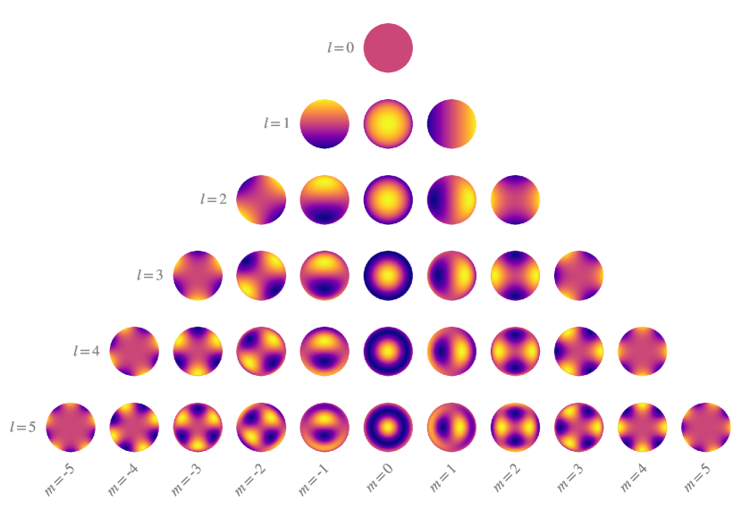
Figure 1: The real spherical harmonics in the polar frame up to $l=5$, where dark colors correspond to negative intensity and bright colors to positive intensity. Rows correspond to the degree $l$ and columns to the order $m$. The set of all spherical harmonics forms a complete, orthogonal basis on the sphere.   

Before we dive into the computation of our GP, it is useful to introduce the spherical harmonics, a set of orthogonal functions on the surface of the sphere which we will use to describe the intensity field on the surface of a star (Figure 1). As we will see below, the spherical harmonics are a particularly convenient basis in which to describe starspot distributions, as they will allow us to compute moments of the intensity distribution analytically. Of more immediate concern, Luger et al. (2019) showed that there is a linear relationship between the spherical harmonic expansion of a stellar surface and the total disk-integrated flux $\mathbf{f}$ (i.e., the light curve) one would observe as the star rotates about a fixed axis. If the stellar surface intensity is described by a spherical harmonic coefficient vector $\mathbf{y}$ (up to a certain degree $l_{\mathrm{max}}$), the flux is given by

$$\mathbf{f}=\mathbf{1}+\boldsymbol{\mathcal{A}}(I,P,\mathbf{u})\,\mathbf{y}\hskip 0.0pt,$$ (3)

where $\mathbf{1}$ is the ones vector and $\boldsymbol{\mathcal{A}}$ is the starry design matrix, a purely linear operator that transforms from the spherical harmonic basis to the flux basis; it is a function of the stellar inclination $I$, the stellar rotation period $P$, and the stellar limb darkening coefficients $\mathbf{u}$, as well as the observation times (see Appendix LABEL:sec:starry for details).

2.3 Computing the GP

Let $\mathbbb{f}=\left(\mathbb{f}_{0}\,\,\mathbb{f}_{1}\,\,\cdots\,\,\mathbb{f}_{K-1}\right)^{\top}$ denote a random vector of $K$ flux measurements at times $\mathbf{t}=\left(t_{0}\,\,t_{1}\,\,\cdots\,\,t_{K-1}\right)^{\top}$, defined in units such that a star with no spots on it will have unit flux. Conditioned on the stellar inclination $I$, the rotational period $P$, a set of limb darkening coefficients $\mathbf{u}$, and on certain properties of the starspots $\boldsymbol{\theta}_{\bullet}$ (including their number, sizes, positions, and contrasts), we wish to compute the mean $\boldsymbol{\mu}(I,P,\mathbf{u},\boldsymbol{\theta}_{\bullet})$ and covariance $\boldsymbol{\Sigma}(I,P,\mathbf{u},\boldsymbol{\theta}_{\bullet})$ of $\mathbbb{f}$. Together, these specify a multidimensional Gaussian distribution, which we assume fully describes how our flux measurements are distributed:

$$\mathbbb{f}\left(I,P,\mathbf{u},\boldsymbol{\theta}_{\bullet}\right)\sim\mathcal{N}\Big{(}\boldsymbol{\mu}\left(I,P,\mathbf{u},\boldsymbol{\theta}_{\bullet}\right),\,\boldsymbol{\Sigma}\left(I,P,\mathbf{u},\boldsymbol{\theta}_{\bullet}\right)\Big{)}$$ (4)

As with any random variable, the mean and covariance may be computed from the expectation values of $\mathbbb{f}$ and $\mathbbb{f}\,\mathbbb{f}^{\top}$, respectively:

$$\boldsymbol{\mu}(I,P,\mathbf{u},\boldsymbol{\theta}_{\bullet}) =\mathrm{E}\Big{[}\mathbbb{f}\,\Big{|}\,I,P,\mathbf{u},\boldsymbol{\theta}_{\bullet}\Big{]}$$ (5)

$$\boldsymbol{\Sigma}(I,P,\mathbf{u},\boldsymbol{\theta}_{\bullet}) =\mathrm{E}\Big{[}\mathbbb{f}\,\mathbbb{f}^{\top}\,\Big{|}\,I,P,\mathbf{u},\boldsymbol{\theta}_{\bullet}\Big{]}-\boldsymbol{\mu}(I,P,\mathbf{u},\boldsymbol{\theta}_{\bullet})\boldsymbol{\mu}^{\top}(I,P,\mathbf{u},\boldsymbol{\theta}_{\bullet})\hskip 0.0pt.$$ (6)

Given the linear relationship between flux and spherical harmonic coefficients (Equation 3), we may write the mean and covariance of our GP as

$$\boldsymbol{\mu}(P,\mathbf{u},\boldsymbol{\theta}_{\bullet}) =\mathbf{1}+\boldsymbol{\mathcal{A}}(I,P,\mathbf{u})\,\boldsymbol{\mu}_{\mathbf{y}}(\boldsymbol{\theta}_{\bullet})$$ (7)

$$\boldsymbol{\Sigma}(P,\mathbf{u},\boldsymbol{\theta}_{\bullet}) =\boldsymbol{\mathcal{A}}(I,P,\mathbf{u})\,\boldsymbol{\Sigma}_{\mathbf{y}}(\boldsymbol{\theta}_{\bullet})\,\boldsymbol{\mathcal{A}}^{\top}(I,P,\mathbf{u})\hskip 0.0pt,$$ (8)

where

$$\boldsymbol{\mu}_{\mathbf{y}}(\boldsymbol{\theta}_{\bullet}) =\mathrm{E}\Big{[}\mathbbb{y}\,\Big{|}\,\boldsymbol{\theta}_{\bullet}\Big{]}$$ (9)

$$\boldsymbol{\Sigma}_{\mathbf{y}}(\boldsymbol{\theta}_{\bullet}) =\mathrm{E}\Big{[}\mathbbb{y}\,\mathbbb{y}^{\top}\,\Big{|}\,\boldsymbol{\theta}_{\bullet}\Big{]}-\boldsymbol{\mu}_{\mathbf{y}}(\boldsymbol{\theta}_{\bullet})\boldsymbol{\mu}_{\mathbf{y}}^{\top}(\boldsymbol{\theta}_{\bullet})$$ (10)

are the mean and covariance of the distribution over spherical harmonic coefficient vectors $\mathbbb{y}$. The bulk of the math in this paper (Appendix LABEL:sec:integrals) is devoted to computing the expectations in the expressions above, which are given by the integrals

$$\mathrm{E}\Big{[}\mathbbb{y}\,\Big{|}\,\boldsymbol{\theta}_{\bullet}\Big{]} =\int\mathbbb{y}(\mathbbb{x})\,p(\mathbbb{x}\,\big{|}\,\boldsymbol{\theta}_{\bullet})\mathrm{d}\mathbbb{x}$$ (11)

$$\mathrm{E}\Big{[}\mathbbb{y}\,\mathbbb{y}^{\top}\,\Big{|}\,\boldsymbol{\theta}_{\bullet}\Big{]} =\int\mathbbb{y}(\mathbbb{x})\mathbbb{y}^{\top}(\mathbbb{x})\,p(\mathbbb{x}\,\big{|}\,\boldsymbol{\theta}_{\bullet})\mathrm{d}\mathbbb{x}\hskip 0.0pt,$$ (12)

where $\mathbbb{x}$ is a random vector-valued variable corresponding to a particular distribution of features on the surface and $p(\mathbbb{x}\,\big{|}\,\boldsymbol{\theta}_{\bullet})$ is its probability density function (PDF). In the Appendix we show that for suitable choices of $\boldsymbol{\theta}_{\bullet}$, $\mathbbb{y}(\mathbbb{x})$, and $p(\mathbbb{x}\,\big{|}\,\boldsymbol{\theta}_{\bullet})$, the integrals in the expressions above have closed form solutions that may be evaluated quickly. While we present a few different ways of specifying $\boldsymbol{\theta}_{\bullet}$, our default representation of the GP hyperparameters is

$$\boldsymbol{\theta}_{\bullet} =\left(n\,\,\,c\,\,\,\mu_{\phi}\,\,\,\sigma_{\phi}\,\,\,r\right)^{\top}\hskip 0.0pt,$$ (13)

where $n$ is the number of starspots, $c$ is their contrast (defined as the intensity difference between the spot and the background intensity, as a fraction of the background intensity), $\mu_{\phi}$ and $\sigma_{\phi}$ are the mode and standard deviation of the spot latitude distribution, respectively, and $r$ is the radius of the spots. For simplicity, the PDFs for the spot radius, the spot contrast, and the number of spots are chosen to be delta functions centered at $r$, $c$, and $n$, respectively (Appendices LABEL:sec:size and LABEL:sec:contrast), while the spot longitude is assumed to be uniformly distributed (Appendix LABEL:sec:lon). Finally, the PDF for the latitude $\phi$ of the spots is chosen to be a Beta distribution in $\cos\phi$ with (normalized) parameters $a$ and $b$, which have a one-to-one correspondence to the mode $\mu_{\phi}$ and standard deviation $\sigma_{\phi}$ of the distribution in $\phi$ (Appendix LABEL:sec:lat). This allows us to model starspot distributions with “active latitudes” of tunable width that are symmetric about the equator. The distribution is flexible enough to also model equatorial spots and isotropically-distributed spots. Stars with multiple active latitudes can easily be modeled as a sum of Gaussian processes (§5.1). These choices for the spatial distribution of spots are based on the Sun, whose spots emerge in azimuthally-symmetric belts at roughly the same latitude in both hemispheres, then migrate toward the equator over the course of the 11-year cycle (Solanki et al., 2006).

In this paper, we assume that the parameters $\boldsymbol{\theta}_{\bullet}$ described above are the physically interesting ones. That is, given a light curve $\mathbf{f}$ or an ensemble of $M$ light curves of statistically similar stars $\left(\mathbf{f}_{0}\,\,\mathbf{f}_{1}\,\,\cdots\,\,\mathbf{f}_{M-1}\right)^{\top}$, we wish to infer the statistical properties of the starspots, encoded in the entries of the vector $\boldsymbol{\theta}_{\bullet}$. This is typically a tall order, since it requires marginalizing over all the nuisance parameters, which include the nitty-gritty details of the size, contrast, and location of every spot (and, if $M>1$, on every star in the ensemble). Fortunately, however, the Gaussian process we constructed does just that. Specifically, given the mean and covariance of the process, we are able to directly evaluate the log marginal likelihood of the $m^{\mathrm{th}}$ dataset conditioned on a specific value of $\boldsymbol{\theta}_{\bullet}$ (as well as $I$, $P$, and $\mathbf{u}$):

$$\ln\mathcal{L}_{m}\left(I,P,\mathbf{u},\boldsymbol{\theta}_{\bullet}\right)= -\frac{1}{2}\mathbf{r}_{m}^{\top}\left(I,P,\mathbf{u},\boldsymbol{\theta}_{\bullet}\right)\big{[}\boldsymbol{\Sigma}\left(I,P,\mathbf{u},\boldsymbol{\theta}_{\bullet}\right)+\mathbf{C}_{m}\big{]}^{-1}\mathbf{r}_{m}\left(I,P,\mathbf{u},\boldsymbol{\theta}_{\bullet}\right)$$

$$-\frac{1}{2}\ln\Big{|}\boldsymbol{\Sigma}\left(I,P,\mathbf{u},\boldsymbol{\theta}_{\bullet}\right)+\mathbf{C}_{m}\Big{|}-\frac{K}{2}\ln\left(2\pi\right)\hskip 0.0pt,$$ (14)

where

$$\mathbf{r}_{m}\left(I,P,\mathbf{u},\boldsymbol{\theta}_{\bullet}\right) \equiv\mathbf{f}_{m}-\boldsymbol{\mu}\left(I,P,\mathbf{u},\boldsymbol{\theta}_{\bullet}\right)$$ (15)

is the residual vector, $\mathbf{C}_{m}$ is the data covariance (which in most cases is a diagonal matrix whose entries are the squared uncertainty corresponding to each data point in the light curve), $|\cdots|$ denotes the determinant, and $K$ is the number of data points in each light curve. In an ensemble analysis, the joint marginal likelihood of all datasets is simply the product of the individual likelihoods, so in log space we have

$$\ln\mathcal{L}\left(I,P,\mathbf{u},\boldsymbol{\theta}_{\bullet}\right) =\sum_{m}\ln\mathcal{L}_{m}\left(I,P,\mathbf{u},\boldsymbol{\theta}_{\bullet}\right)\hskip 0.0pt.$$ (16)

The marginal likelihood may be interpreted as the probability of the data given the model. Typically, we are interested in the reverse: the probability of the model given the data, i.e., the posterior probability distribution. In later sections we present a comprehensive suite of posterior inference exercises demonstrating that our GP model is correctly calibrated, allowing one to efficiently infer statistical properties of starspots from light curves with minimal bias.

2.4 Marginalizing over inclination

As we mentioned in the previous section, the equations for the mean and covariance of our GP (Equations 7 and 8, respectively) are conditioned on specific values of the stellar and spot properties. To obtain the posterior distribution for these parameters, we must typically resort to numerical sampling techniques, which often scale steeply with the number of parameters. It is therefore generally desirable to keep the total number of parameters small, especially when employing the GP in an ensemble setting. In such a setting, we might have light curves from $M$ stars, all of which we believe to have similar spot properties (perhaps because they have similar spectral types and rotation periods, for example). The total number of parameters in our problem is therefore

$$N=4M+5\hskip 0.0pt,$$ (17)

since each of the stars will have their own set of 4 stellar properties (an inclination, a period, and usually two limb darkening coefficients) but will all share the same 5 spot properties $\boldsymbol{\theta}_{\bullet}$ (by assumption). For a reasonably sized ensemble of $M=100$ stars, we would have to sample over $N=405$ parameters. While large, this number is certainly not absurd, especially by modern standards. However, it does pose a problem when considering how complex the posterior distribution for the spot mapping problem can be. In addition to strong nonlinear degeneracies between some of the parameters (such as the contrast $c$ and the number of spots $n$), the posterior is often multimodal, especially in the stellar inclinations. While modern sampling schemes such as Hamiltonian Monte Carlo and Nested Sampling may in principle be able to deal with these issues, in practice it can be very difficult to obtain convergence in a reasonable amount of time.

One workaround is to fix the values of the stellar parameters. This could be done, for instance, to the rotational period $P$, which can often be estimated with fairly good accuracy from a periodogram. The limb darkening coefficients could be fixed at theoretical values, or perhaps their values could be shared among all stars (and sampled over), given the similarity assumption above.

The inclination, however, is a different matter. Absent prior information for a particular star (such as a measurement of its projected rotational velocity $v\sin I$ or the knowledge that it hosts a transiting planet), it is simply not possible to reliably estimate the inclination in a pre-processing step. Any light curve statistic one might argue should scale with inclination—such as the amplitude of the variability—is invariably degenerate with the spot parameters $\boldsymbol{\theta}_{\bullet}$. If one knew $\boldsymbol{\theta}_{\bullet}$, then perhaps a decent point estimate of $I$ could be obtained, but in that case the analysis wouldn’t be needed in the first place!

Fortunately, there is a better way to reduce the number of parameters in the problem: we can explicitly marginalize over the stellar inclination. That is, we may write the mean and covariance of our GP as

$$\boldsymbol{\mu}(P,\mathbf{u},\boldsymbol{\theta}_{\bullet}) =\mathrm{E}\Big{[}\mathbbb{f}\,\Big{|}\,P,\mathbf{u},\boldsymbol{\theta}_{\bullet}\Big{]}$$

$$=\mathbf{1}+\mathbf{e}_{I}$$ (18)

$$\boldsymbol{\Sigma}(P,\mathbf{u},\boldsymbol{\theta}_{\bullet}) =\mathrm{E}\Big{[}\mathbbb{f}\,\mathbbb{f}^{\top}\,\Big{|}\,P,\mathbf{u},\boldsymbol{\theta}_{\bullet}\Big{]}-\boldsymbol{\mu}(P,\mathbf{u},\boldsymbol{\theta}_{\bullet})\boldsymbol{\mu}^{\top}(P,\mathbf{u},\boldsymbol{\theta}_{\bullet})$$

$$=\mathbf{E}_{I}-\mathbf{e}_{I}\,\mathbf{e}_{I}^{\top}$$ (19)

where we define the inclination first moment integral

$$\mathbf{e}_{I} \equiv\int\boldsymbol{\mathcal{A}}(\mathbb{I},P,\mathbf{u})\,\mathrm{E}\Big{[}\mathbbb{y}\,\Big{|}\,\boldsymbol{\theta}_{\bullet}\Big{]}p(\mathbb{I})\,\mathrm{d}\mathbb{I}$$ (20)

and the inclination second moment integral

$$\mathbf{E}_{I} \equiv\int\boldsymbol{\mathcal{A}}(\mathbb{I},P,\mathbf{u})\,\mathrm{E}\Big{[}\mathbbb{y}\,\mathbbb{y}^{\top}\,\Big{|}\,\boldsymbol{\theta}_{\bullet}\Big{]}\,\boldsymbol{\mathcal{A}}^{\top}(\mathbb{I},P,\mathbf{u})p(\mathbb{I})\,\mathrm{d}\mathbb{I}\hskip 0.0pt,$$ (21)

and $\mathbb{I}$ is the random variable corresponding to the inclination. The expectations inside the integrals in the expressions for $\mathbf{e}_{I}$ and $\mathbf{E}_{I}$ are given by Equations (11) and (12), respectively, and are computed in Appendix LABEL:sec:integrals. If we are able to perform the integrals in those expressions, we can dramatically reduce the number of parameters in our ensemble problem. As we show in Appendix 2.4, if we assume that stellar inclinations are distributed isotropically, these integrals do in fact have closed-form solutions.

Finally, for future reference, it is useful to note that the mean of the GP is constant:

$$\boldsymbol{\mu}(P,\mathbf{u},\boldsymbol{\theta}_{\bullet}) =(1+e_{I})\mathbf{1}$$

$$\equiv\mu\,\mathbf{1}\hskip 0.0pt,$$ (22)

since by construction our GP is longitudinally isotropic (see Appendix LABEL:sec:inc-mom1).

2.5 Normalization correction

In Paper I we discussed a subtle but important point about stellar light curves: the common procedure of normalizing light curves to their mean or median level changes the covariance structure of the data, since it correlates all the observations in a nontrivial way. When normalizing a light curve by the mean, the operation we perform is

$$\tilde{\mathbbb{f}\hskip 1.99997pt} =\frac{\mathbbb{f}}{\left<\mathbb{f}\right>}\hskip 0.0pt,$$ (23)

where $\tilde{\mathbbb{f}\hskip 1.99997pt}$ is the normalized, unit-mean light curve, $\mathbbb{f}$ is the measured light curve (in detector counts), and $\left<\mathbb{f}\right>$ is the sample mean: i.e., the average value of a given star’s light curve (which we model as a sample from our GP). This may be close to but is in general different from the process mean, $\boldsymbol{\mu}(P,\mathbf{u},\boldsymbol{\theta}_{\bullet})$, since the mean of a draw from the GP is itself normally distributed with a variance that scales with the GP variance.

When modeling normalized light curves, we must correct our expression for the covariance matrix $\boldsymbol{\Sigma}$ of the GP. Computing the new covariance matrix is tricky, especially because the normalized process is not strictly Gaussian: the distribution of normalized light curves has heavy tails due to the fact that $\tilde{\mathbbb{f}\hskip 1.99997pt}$ diverges as the sample mean approaches zero. In fact, because of these tails, the covariance of the normalized process is formally infinite, since the probability of drawing a sample whose mean is arbitrarily close to zero is finite.

If this is all starting to sound like a bad idea, that’s because it is! A much safer approach is to resist the temptation to normalize the light curve and instead model the (unknown) amplitude of the data as a multiplicative latent variable. However, this would require an extra parameter for every light curve, so the computational savings we achieved by marginalizing out the inclination would be gone. Fortunately, in practice, the variance of a stellar light curve is usually small compared to its mean: stellar variability amplitudes are typically at the level of a few percent or lower. When this is the case, the probability of drawing a GP sample whose mean is close to zero is extremely small, and we can make use of the approximate expression derived in Luger (2021) for the covariance of a normalized Gaussian process:

$$\tilde{\boldsymbol{\Sigma}} \approx\frac{A}{\mu^{2}}\boldsymbol{\Sigma}+z\Big{(}(A+B)\,(\mathbf{1}-\mathbf{q})\,(\mathbf{1}-\mathbf{q})^{\top}-A\,\mathbf{q}\,\mathbf{q}^{\top}\Big{)}\hskip 0.0pt,$$  (24)

where

$$z \equiv\frac{\left<\Sigma\right>}{\mu^{2}}$$ (25)

is the ratio of the average element in $\boldsymbol{\Sigma}$ to the square of the mean of the Gaussian process, $\mathbf{q}$ is the ratio of the average of each row in $\boldsymbol{\Sigma}$ to the average element in $\boldsymbol{\Sigma}$, and $A$, $B$ are order unity and zero scalars, respectively, given by the optimally-truncated diverging series

$$A \equiv\sum\limits_{i=0}^{i_{\mathrm{max}}}\frac{(2i+1)!}{2^{i}\,i!}z^{i}$$ (26)

$$B \equiv\sum\limits_{i=0}^{i_{\mathrm{max}}}\frac{2i(2i+1)!}{2^{i}\,i!}z^{i}\hskip 0.0pt,$$ (27)

where $i_{\mathrm{max}}$ is the largest value for which the series coefficient at $i_{\mathrm{max}}$ is smaller than the coefficient at $i_{\mathrm{max}}-1$. In the expressions above, it is assumed that the mean $\boldsymbol{\mu}$ is constant, i.e., $\boldsymbol{\mu}=\mu\,\mathbf{1}$. Since our Gaussian process is azimuthally isotropic (i.e., no preferred longitude), that is the case throughout this paper.

What Equation (24) allows us to do is effectively marginalize over the unknown normalization by modeling the normalized flux as a draw from a Gaussian process:

$$\tilde{\mathbbb{f}\hskip 1.99997pt}\left(P,\mathbf{u},\boldsymbol{\theta}_{\bullet}\right)\sim\mathcal{N}\left(\mathbf{1},\tilde{\boldsymbol{\Sigma}}\left(P,\mathbf{u},\boldsymbol{\theta}_{\bullet}\right)\right)\hskip 0.0pt.$$ (28)

This is appropriate as long as $z\ll 1$, for which the true distribution of $\tilde{\mathbbb{f}\hskip 1.99997pt}$ is approximately Gaussian. In practice, we recommend employing this trick only for $z\lesssim 0.02$, for which the error in the approximation to the covariance is less than $10^{-6}$. In cases where the light curve variability exceeds about ten percent, we recommend modeling the multiplicative amplitude in each light curve as a latent variable, as discussed above.

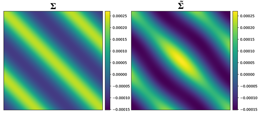
Figure 2: An example of a flux covariance matrix $\boldsymbol{\Sigma}$ for a starry process (left) and the corresponding covariance of the normalized process (right), computed from Equation (24). In addition to an offset and an overall scaling relative to the original covariance matrix, the covariance of the normalized process is discernibly non-stationary.   

Figure 2 shows an example of a covariance matrix normalized according to the procedure outlined above. The principal difference between the normalized covariance and the original covariance is an overall scaling and a small offset. However, the normalization also results in the process becoming non-stationary: the covariance between two points in a light curve is now slightly dependent on their phases.

2.6 Summary

As the computation of the GP relies on many interdependent equations scattered throughout the previous sections and the Appendix, it is useful to summarize the procedure for the case where we marginalize over the inclination (§2.4) and the light curves are normalized to their means (§2.5), which is likely to be the primary use case for our algorithm.

We model the mean-normalized flux $\tilde{\mathbbb{f}\hskip 1.99997pt}$ (Equation 23) as a Gaussian process:

$$\tilde{\mathbbb{f}\hskip 1.99997pt}\left(P,\mathbf{u},\boldsymbol{\theta}_{\bullet}\right)\sim\mathcal{N}\left(\mathbf{1},\tilde{\boldsymbol{\Sigma}}\left(P,\mathbf{u},\boldsymbol{\theta}_{\bullet}\right)\right)\hskip 0.0pt.$$ (29)

The hyperparameters of the GP are the stellar rotation period $P$, the vector of limb darkening coefficients $\mathbf{u}$, and the vector of parameters describing the spot distribution

$$\boldsymbol{\theta}_{\bullet} =\left(n\,\,\,c\,\,\,\mu_{\phi}\,\,\,\sigma_{\phi}\,\,\,r\right)^{\top}\hskip 0.0pt,$$ (30)

consisting of the number of spots $n$, their contrast $c$ (the fractional intensity difference between the background and the spot), the mode $\mu_{\phi}$ and standard deviation $\sigma_{\phi}$ of the latitude distribution, and the radius of the spots $r$. The quantity $\tilde{\boldsymbol{\Sigma}}$ is the covariance of the normalized process (Equation 24), which is a straightforward correction to the true covariance of the process, accounting for changes in scale and phase introduced by the common process of normalizing light curves to a mean of unity. It depends on the true (constant) mean $\mu$ and true covariance $\boldsymbol{\Sigma}$, given by Equations (2.4) and (2.4), respectively. Those expressions in turn depend on the inclination expectation integrals $e_{I}$ (Appendix LABEL:sec:inc-mom1) and $\mathbf{E}_{I}$ (Appendix LABEL:sec:inc-mom2). Those, in turn, depend on the first and second moments of the distribution of spherical harmonic coefficient vectors, $\mathrm{E}\left[\mathbbb{y}\,\big{|}\,\boldsymbol{\theta}_{\bullet}\right]$ and $\mathrm{E}\left[\mathbbb{y}\,\mathbbb{y}^{\top}\,\big{|}\,\boldsymbol{\theta}_{\bullet}\right]$, given by Equations (LABEL:eq:exp_y_sep) and (LABEL:eq:exp_yy_sep), respectively. To compute those, we must evaluate four nested integrals (Equations LABEL:eq:e1–LABEL:eq:e4 for the first moment and LABEL:eq:E1–LABEL:eq:E4 for the second moment), corresponding to integrals over the radius, latitude, longitude, and contrast distributions, respectively. The computation of these integrals is discussed at length in Appendix LABEL:sec:integrals.

While lengthy (and quite tedious), all of the computations described above rely on equations whose solutions have a closed form. Moreover, most of the terms in the expectation vectors and matrices may be computed recursively, and many may be pre-computed, as they do not depend on user inputs. It is therefore possible to evaluate $\tilde{\boldsymbol{\Sigma}}$ in an efficient manner. In the companion paper (Luger et al., 2021a), we discuss our implementation of the algorithm in a user-friendly Python package.

2.7 An example

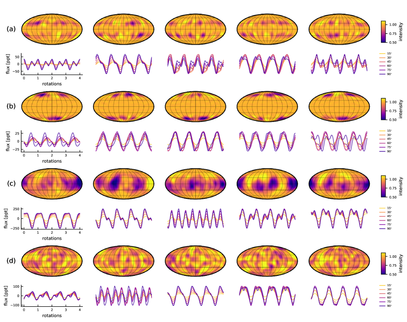
Figure 3: Five random samples from the GP prior (columns) conditioned on four different values of $\boldsymbol{\theta}_{\bullet}$ (rows). The samples are shown on the surface of the star in a Mollweide projection (upper panels) alongside their corresponding light curves viewed over four rotation cycles at several different inclinations (lower panels). From top to bottom, the GP corresponds to a star with (a) small mid-latitude spots; (b) small circumpolar spots; (c) large equatorial spots; and (d) small isotropic spots. See text for details.   

A concrete example of the GP derived above is presented in Figure 3, where we show random samples from the process evaluated up to spherical harmonic degree $l_{\mathrm{max}}=15$ and conditioned on different values of the hyperparameter vector $\boldsymbol{\theta}_{\bullet}$. Each column corresponds to a different random draw from the GP, while each row corresponds to a different value of $\boldsymbol{\theta}_{\bullet}$. The images are intensity maps of the stellar surface seen in an equal-area Mollweide projection, in units such that a spotless star would have intensity equal to 1 everywhere. Below them are the corresponding light curves (in units of parts per thousand deviation from the mean) over four rotation cycles, seen at inclinations varying from $15^{\circ}$ (yellow) to $90^{\circ}$ (dark blue), and assuming no limb darkening (i.e., $\mathbf{u}=\mathbf{0}$). From top to bottom, the hyperparameter vectors $\boldsymbol{\theta}_{\bullet}$ for each row are

$$\left(n\,\,\,c\,\,\,\mu_{\phi}\,\,\,\sigma_{\phi}\,\,\,r\right)^{\top} =\left(10.0\,\,\,\,\,\,\,\,\,0.10\,\,\,\,\,\,\,\,\,30.0\,\,\,\,\,\,\,\,\,5.00\,\,\,\,\,\,\,\,\,10.0\right)^{\top}$$ (31a)

$$=\left(10.0\,\,\,\,\,\,\,\,\,0.10\,\,\,\,\,\,\,\,\,60.0\,\,\,\,\,\,\,\,\,5.00\,\,\,\,\,\,\,\,\,10.0\right)^{\top}$$ (31b)

$$=\left(10.0\,\,\,\,\,\,\,\,\,0.05\,\,\,\,\,\,\,\,\,0.00\,\,\,\,\,\,\,\,\,5.00\,\,\,\,\,\,\,\,\,30.0\right)^{\top}$$ (31c)

$$=\left(20.0\,\,\,\,\,\,\,\,\,0.10\,\,\,\,\,\,\,\,\,0.00\,\,\,\,\,\,\,\,\,40.0\,\,\,\,\,\,\,\,\,10.0\right)^{\top}\hskip 0.0pt.$$ (31d)

These correspond to (a) 10 spots of radius $10^{\circ}$ centered at $30^{\circ}\pm 5^{\circ}$ latitude with a contrast of $10\%$; (b) 10 spots of radius $10^{\circ}$ centered at $60^{\circ}\pm 5^{\circ}$ latitude with a contrast of $10\%$; (c) 10 spots of radius $30^{\circ}$ centered at $0^{\circ}\pm 5^{\circ}$ latitude with a contrast of $5\%$; and (d) 20 spots of radius $10^{\circ}$ centered at $0^{\circ}\pm 40^{\circ}$ latitude (a good approximation to a perfectly isotropic distribution; see Appendix LABEL:sec:lat) with a contrast of $10\%$.

The surface maps in the figure show dark, compact features of roughly the expected size and contrast and at the expected latitudes. However, there are important differences between these maps and what we would obtain by procedurally adding discrete circular spots to a gridded stellar surface:

1. The spots are not circular. This is most evident in row (c), where some spots are distinctly asymmetric.

2. There is significant variance in contrast from one spot to another, even though our model implicitly treats $c$ as constant. Within spots, the contrast is also not constant, even though (again) our model implictly treats it as such.

3. There is ringing in the background. This is apparent to some extent in row (b), where there are small fluctuations in the brightness at low latitudes where no spots are present.

4. There aren’t exactly 10 (or 20) spots in those maps. This is most obvious in row (c), where only a few large distinct spots, plus maybe a few smaller ones, are visible.

5. There are bright spots in addition to dark spots. This may be the most glaring issue. We explicitly model spots as being dark, and yet there are (almost) just as many bright spots, particularly in row (d). While bright spots (such as plages) certainly exist in reality, we did not explicitly ask for them here!

While these may appear to be critical shortcomings of our model, it is important to keep in mind that a model consisting of discrete, circular, constant contrast spots is likely just as far (or perhaps even farther) from the truth. In fact, points (1) and (2) above suggest our model is more flexible than the discrete spot model and thus (potentially) better suited to modeling real stellar surfaces. Points (3), (4), and (5), on the other hand, are more concerning, since they are due, respectively, to truncation error in the spherical harmonic expansion, to an intrinsic limitation of our Gaussian approximation, and to the fact that Gaussian distributions are symmetric about the mean: a positive deviation is just as likely as a negative deviation of the same magnitude. However, as we have argued before, the true power of the GP is in its applicability to inference problems. In other words, while our GP has some undesirable features when used as a prior sampling distribution, the real test of the GP is when it is faced with data in an inference setting. As long as the data is sufficiently informative, it does not matter that the prior has finite support for unphysical configurations, as those will be confidently rejected.

In §3 below, we exhaustively test the performance of our GP as an inference tool when used to model synthetic light curves. We will show that, despite the issues raised above, the GP is in general unbiased and correctly estimates the posterior variance when used to infer the spot properties $\boldsymbol{\theta}_{\bullet}$.

But before we dive into calibration tests, it is worth pausing for a moment to take another look at Figure 3. While we focused on the shortcomings of the GP as a prior in the discussion above, it is important to appreciate that it even works in the first place! A Gaussian process, after all, is a non-parameteric process describing a smooth and continuous function only via its covariance structure. The GP knows nothing about the existence of discrete spots—only how any two points on the surface are correlated. Because spherical harmonics are smooth functions with support over the entire sphere, the GP also does not know about features restricted to certain latitudes; in fact, in most applications of GPs to mapping problems in astronomy (such as in models of the cosmic microwave background; e.g., Wandelt, 2012), the process is assumed to be isotropic, with no preferred angular direction. However, by prescribing the correct structure to the covariance matrix, we are able to approximately model compact spot-like features with given sizes and restricted to particular latitudes.

3 Calibration

3.1 Why we need calibration tests

In the previous section we derived a closed form solution to the Gaussian approximation to the distribution of stellar surfaces (and their corresponding light curves) conditioned on a vector $\boldsymbol{\theta}_{\bullet}$ of spot hyperparameters. As we mentioned, the real test of this GP is in how well it performs as a likelihood function for stellar light curves.

Figure 4: Corner plot showing the joint distributions of select spherical harmonic coefficients corresponding to the $l=15$ expansion of $5\times 10^{4}$ stellar surface maps drawn from a certain distribution of discrete circular spots (black points and contours). At $l=15$ there are 256 coefficients in total; we chose five of the coefficients with the most odd-looking distributions to illustrate the non-Gaussianity of the process. In addition to non-linear correlations, skewness, and the existence of points of very high curvature, some of the distributions are also multi-modal. The orange contours show slices of the Gaussian approximation to the joint distribution; this is the approximation adopted in this paper.   

It is not immediately obvious that the GP approach should work, because the true marginal likelihood function $p(\tilde{\mathbbb{f}\hskip 1.99997pt}\,\big{|}\,P,\mathbf{u},\boldsymbol{\theta}_{\bullet})$ is certainly not Gaussian. To see why, let us generate $10^{4}$ stellar surfaces sampled from the true distribution we are trying to model: that is, a surface with $n=5$ discrete circular spots of fixed, uniform contrast $c=0.1$ and radius $r=20^{\circ}$ at latitudes $\mu_{\phi}\pm\sigma_{\phi}=30^{\circ}\pm 5^{\circ}$. Let us then expand each surface in spherical harmonics and visualize the distribution of coefficients $\mathbbb{y}$. Figure 4 shows the joint distribution for five of the coefficients with the most non-Gaussian marginal distributions (selected by eye). Different slices through this distribution (in black) are skewed, strongly peaked, non-linearly correlated, and even bimodal. Our approach in this paper is to model this distribution as a Gaussian (orange contours). While this may be a good approximation in certain regions of parameter space, it is certainly a poor approximation in others. In this section, we will show that, fortunately, the non-Gaussianity of the distribution is not in general an issue when doing inference with our GP, as the resulting posteriors are correctly calibrated.

3.2 Setup

Symbol	Description	Value
$\mathbb{n}$	number of spots	$\sim\mathcal{N}(20,0^{2})$
$\mathbb{c}$	spot contrast	$\sim\mathcal{N}(0.05,0^{2})$
$\bbphi$	spot latitude	$\sim\mathcal{N}(30^{\circ},{5^{\circ}}^{2})$
$\bblambda$	spot longitude	$\sim\mathcal{U}(0^{\circ},360^{\circ})$
$\mathbb{r}$	spot radius	$\sim\mathcal{N}(15^{\circ},{0^{\circ}}^{2})$
$\mathbb{I}$	stellar inclination	$\sim\sin$
$P$	rotational period	$1$ day
$\mathbf{u}$	limb darkening coefficients	$\left(0\,\,\,\,0\right)^{\top}$
$\sigma_{f}$	photometric uncertainty	$10^{-3}$
$K$	number of cadences per light curve	$10^{3}$
$\Delta t$	time baseline	$4$ days
$M$	number of light curves in ensemble	$50$

Table 1: Default parameters used to generate synthetic light curves in the calibration tests.

We seek to demonstrate that our model is correctly calibrated by testing it on synthetic data, which we generate as follows. For each of $M$ synthetic light curves in a given ensemble, we create a rectangular $(150\times 300)$ latitude-longitude grid of surface intensity values, all intialized to zero. We then add $\mathbb{n}$ spots to this grid, each of fractional contrast $\mathbb{c}$ and radius $\mathbb{r}$ centered at latitude $\bbphi$ and longitude $\bblambda$, by decreasing the intensity at all points within an angular distance $\mathbb{r}$ (measured along the surface of the sphere) by an amount $\mathbb{c}$. In order to compute the corresponding light curve, we expand the surface in spherical harmonics, although at much higher degree ($l_{\mathrm{max}}^{(0)}=30$) than the degree we will use in the inference step ($l_{\mathrm{max}}=15$) to minimize potential ringing effects or other artefacts in the synthetic data. For reference, the chosen degree $l_{\mathrm{max}}=30$ is large enough to resolve features on the order of $\nicefrac{{180^{\circ}}}{{30}}=6^{\circ}$ across, but small enough that the algorithm for computing the light curve is numerically stable. We compute the light curve at $K$ points equally spaced over a baseline $\Delta t$ using the starry algorithm (Appendix LABEL:sec:starry), assuming an inclination $\mathbb{I}$, a rotational period $P$, and limb darkening coefficients $\mathbf{u}$. Finally, we divide the light curve by the mean and add Gaussian noise with standard deviation $\sigma_{f}$ to emulate photon noise. The default values/distributions of each of the parameters mentioned above are given in Table LABEL:tab:synthetic. Some, like the number of spots, their contrast, etc., are drawn from fiducial distributions, while others, like the photometric uncertainty, the rotational period, and the limb darkening coefficients, are fixed across all $M$ light curves in an ensemble. These fixed values are not realistic, but they greatly speed up the inference step, since they allow us to invert a single covariance matrix for all light curves when computing the log likelihood.

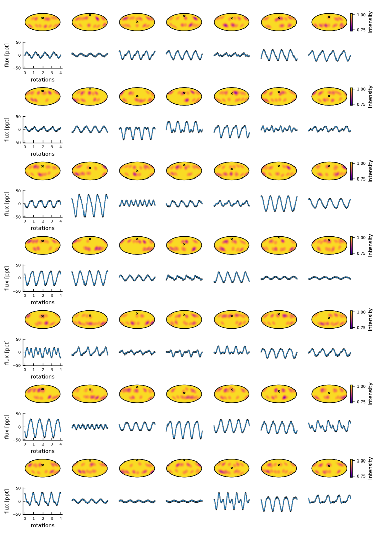
Figure 5: A synthetic dataset generated by adding discrete spots to a stellar surface with parameters given by the default values listed in Table LABEL:tab:synthetic. The surface maps for 49 synthetic stars are shown in a Mollweide equal-area projection above their corresponding light curves. All maps and light curves are plotted on the same scale. The $\times$ on each map indicates the sub-observer latitude assumed when generating the light curve. The blue curves correspond to the exact light curve, while the black dots are the observed light curve.   

Figure 5 shows a synthetic dataset generated from the default values listed in Table LABEL:tab:synthetic. While the light curves correspond to surfaces with the same statistical spot properties, they all look qualitatively different: the mapping from starspot properties to flux is nontrivial. In the inference step below, we assume we observe only these 50 light curves (the figure only shows 49 of them), with no knowledge of the inclination of any individual star, and attempt to infer the spot properties.

3.3 Inference

We use our Python-based implementation of the GP (Luger et al., 2021a) to perform inference on the synthetic datasets. For simplicity, we assume we know the value of the period $P$, which is fixed at unity for all stars, as well as the value of the limb darkening coefficients (fixed at zero for the default run). In practice these will not be known exactly; we discuss this further in §5.3. Since we explicitly marginalize over the inclinations of individual stars, the only quantities we must constrain are the five parameters in the spot parameter vector $\boldsymbol{\theta}_{\bullet}$ (Equation 13). We experimented with three different methods for doing posterior inference on our synthetic datasets: No-U Turn Sampling, a variant of Hamiltonian Monte Carlo (NUTS; Duane et al., 1987; Hoffman & Gelman, 2011), automatic differentiation variational inference (ADVI; Kucukelbir et al., 2016; Blei et al., 2016), and nested sampling (Skilling, 2004, 2006). We obtained the best performance using the nested sampling algorithm implemented in the dynesty package (Speagle, 2020), so that is what we will use below.

Our sampling parameters are the number of spots $n$, their contrast $c$, their radius $r$, and the Beta distribution parameters $a$ and $b$ describing their distribution in latitude. As we discuss in Appendix LABEL:sec:lat, the parameters $a$ and $b$ are easier to sample in than the mode $\mu_{\phi}$ and standard deviation $\sigma_{\phi}$, provided we account for the Jacobian of the transformation (Equation LABEL:eq:J) in our log probability function, which maps a uniform prior on $a$ and $b$ to a uniform prior on $\mu_{\phi}$ and $\sigma_{\phi}$.

We place uniform priors on all five quantities, with support in $1\leq n\leq 50$, $0<c\leq 1$, $10^{\circ}\leq r\leq 30^{\circ}$, $0\leq a\leq 1$, and $0\leq b\leq 1$. Note that while $n$ formally represents an integer, its effect on the GP is a scaling of the covariance (see Equation LABEL:eq:exp_yy_sep); as such, it has support over all real numbers within the bounds listed above. We could restrict it to integer values, but this would make sampling quite tricky. Moreover, in practice it is useful to allow for noninteger values to add some flexibility to the model; we discuss this in more detail in §4.4.

We use Equation (2.3) as our log likelihood term, adding the log of the absolute value of Equation (LABEL:eq:J) to enforce a uniform prior on $\mu_{\phi}$ and $\sigma_{\phi}$. As we mentioned above, the fact that $P$, $\mathbf{u}$, and $\sigma_{f}$ are shared among all $M$ light curves means that $\boldsymbol{\Sigma}+\mathbf{C}_{m}$ is the same for all of them, greatly speeding up the likelihood evaluation since we need only invert (or factorize) it a single time per sample. Our covariance is the covariance of the normalized process, given by Equation (24). Since we only consider light curves with variability limited to a few percent or less, the approximation for $\tilde{\boldsymbol{\Sigma}}$ is always valid. Finally, we restrict our spherical harmonic expansion to $l_{\mathrm{max}}=15$ as a compromise between resolution, computational speed, and numerical stability (see Luger et al., 2021a).

We use the standard implementation of the nested sampler, dynesty.NestedSampler, with all arguments set to their default values (multi-ellipsoidal decomposition for bounds determination (Feroz et al., 2009), uniform sampling within the bounds, 500 live points, and no gradients), to perform our inference step. Convergence—defined as when the estimate of the remaining evidence $\Delta\ln\mathcal{Z}$ drops below $0.5$—is usually attained after $5{,}000$ to $10{,}000$ samples and within a couple hours on a typical machine for most of the trials we perform.

Below we describe several calibration runs: experiments where we generate an ensemble of light curves from synthetic stars with given properties (§3.2) and attempt to infer their statistical spot properties.

3.4 Default run

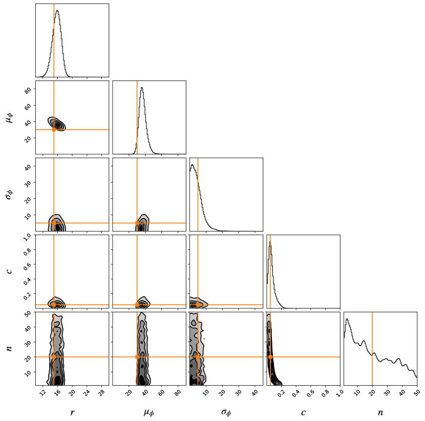
Figure 6: Posterior distributions for the spot parameters $\boldsymbol{\theta}_{\bullet}$ (radius $r$ in degrees, latitude mode $\mu_{\phi}$ and standard deviation $\sigma_{\phi}$ in degrees, fractional contrast $c$, and number of spots $n$) for the default run (Table LABEL:tab:synthetic and Figure 5). The axes span the entire prior volume, and the orange lines and markers indicate the true (input) values.   

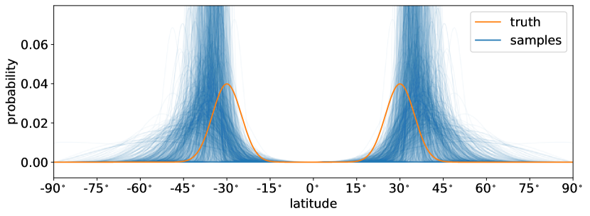
Figure 7: Posterior distributions for the spot latitudes for the default run. Each blue curve corresponds to the Beta distribution PDF (Equation LABEL:eq:phi-pdf) for the spot latitude with parameters drawn from the posterior in $\mu_{\phi}$ and $\sigma_{\phi}$ (Figure 6); the (hyper)distribution of blue curves quantifies our beliefs about how spots are distributed on any given star. The orange curve is the true distribution used to generate the spots (see Table LABEL:tab:synthetic).   

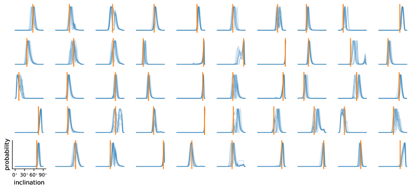
Figure 8: Posterior distributions for the inclinations of individual stars; individual panels correspond directly to those in Figure 5. As in Figure 7, each blue curve is a sample from the hyperdistribution of inclination PDFs, conditioned on a specific value of $\boldsymbol{\theta}_{\bullet}$ drawn from the posterior. The orange lines indicate the true inclination of each star.   

The input parameters for the default run are shown in Table LABEL:tab:synthetic, and the corresponding light curves in Figure 5. We run the nested sampler as described in the previous section and transform the posteriors in $a$ and $b$ to posteriors in $\mu_{\phi}$ and $\sigma_{\phi}$ via Equations (LABEL:eq:beta2gauss), (LABEL:eq:muphi), and (LABEL:eq:sigmaphi). The results are shown in Figure 6, where we correctly infer all five parameters within $2-3$ standard deviations. Posterior distributions for the spot radius $r$, the central spot latitude $\mu_{\phi}$, and the spot contrast $c$ are fairly tight, while the distribution for the latitudinal scatter $\sigma_{\phi}$ has wider tails and the distribution for the number of spots $n$ is very poorly constrained. The latter, in particular, is degenerate with the spot contrast $c$; we discuss this at length in Paper I.

Figure 7 shows samples from the spot latitude posterior (hyper)distribution. Since the parameters $\mu_{\phi}$ and $\sigma_{\phi}$ characterize a distribution over spot latitudes, uncertainty in their values translates to uncertainty in the actual shape of the spot latitude distribution. Thus, the collection of blue curves in Figure 7 quantifies our knowledge of how spots are distributed on the surfaces of the stars in the dataset. These distributions are again consistent with the true distribution used to generate the spots (orange curve) within less than 2 standard deviations.

Even though we explicitly marginalized over inclination, we can still derive posterior constraints on the inclinations of the individual stars in our ensemble by computing the log-likelihood as a function of $I$ conditioned on the value of $\boldsymbol{\theta}_{\bullet}$ from a particular draw from the posterior. We do this in Figure 8, where blue curves again correspond to samples from the posterior hyperdistribution, and orange lines indicate the true inclination; the panels are arranged in the same order as those in Figure 5. In almost all cases, we are able to constrain the inclinations of individual stars to within about $10^{\circ}$, consistent with the truth at less than $2{-}3\sigma$.

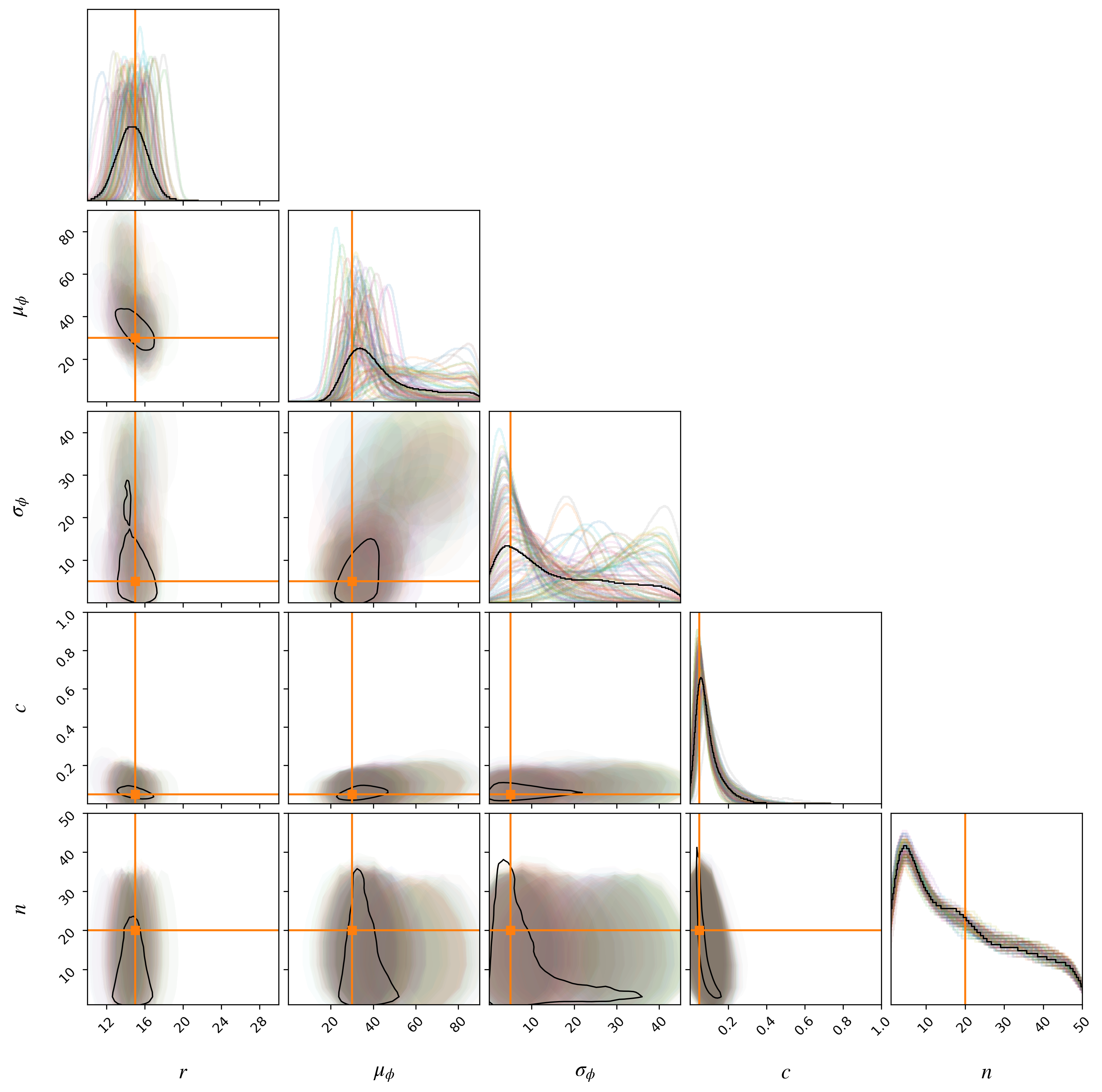
Figure 9: Similar to Figure 6, but showing the posterior distribution for 100 different synthetic datasets, all generated from the same default input parameters (Table LABEL:tab:synthetic). Each colored histogram corresponds to a single run, with the corresponding $1\sigma$ contours shown as shaded ellipses for each pair of parameters. The black histograms correspond to the distributions of all samples from each of the 100 runs, and the black curves again indicate $1\sigma$ contours in the joint posterior.   

Figure 10: Distribution of stellar inclination residuals normalized to the posterior standard deviation for all $5{,}000$ stars across the 100 trials in Figure 9 (blue). The standard normal distribution is shown in orange for comparison. The inclination posteriors inferred with our GP are largely unbiased and have the expected variance.   

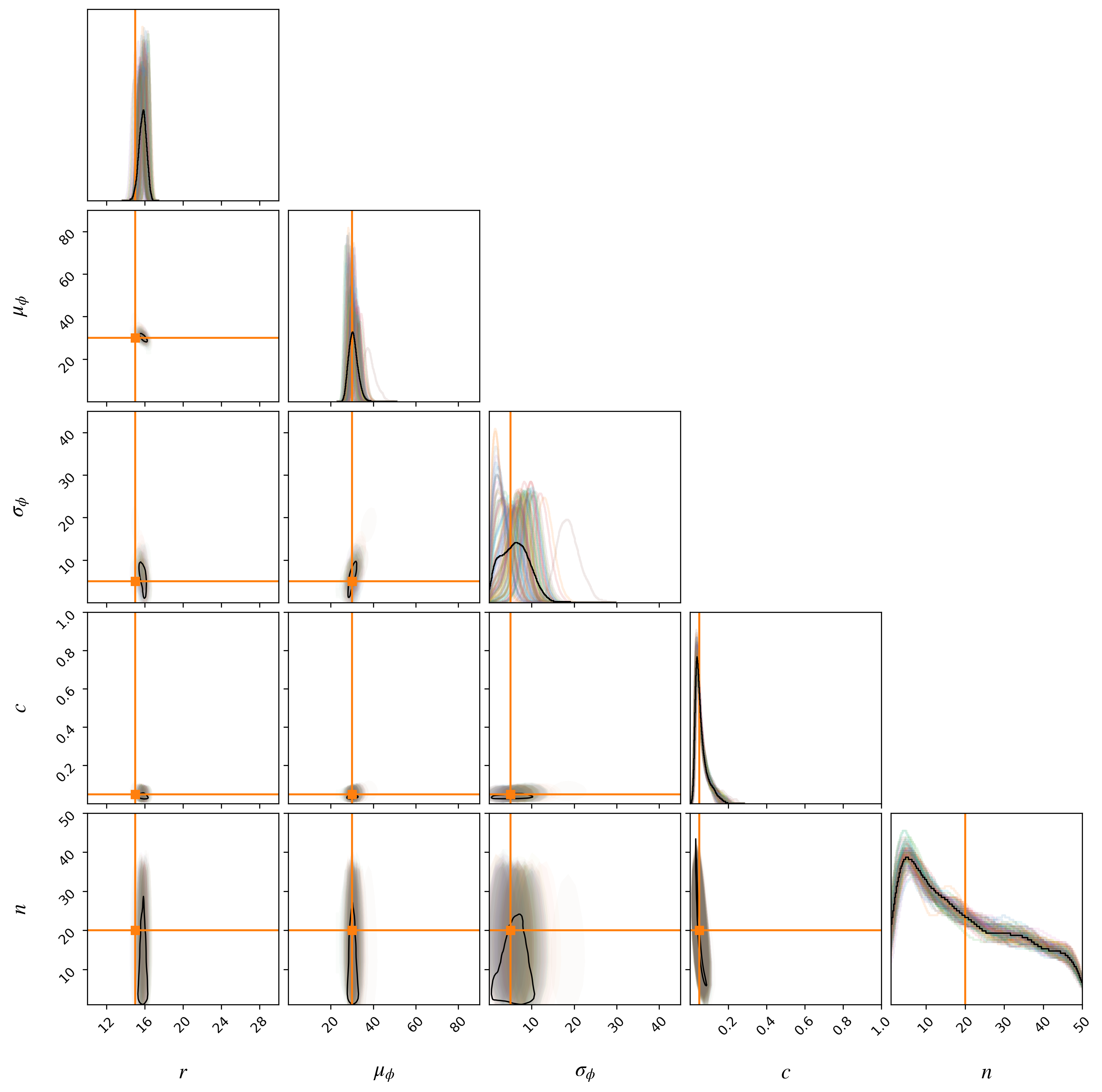
Figure 11: Same as Figure 9, but showing the posterior distributions of 100 realizations of ensembles with $M=1{,}000$ (instead of 50) light curves each. The constraints on mosts of the parameters are much tighter, and the polar spot degeneracy is gone.   

The results in Figures 6—8 are based on a single run: i.e., a single realization of the light curve ensemble conditioned on the properties of Table LABEL:tab:synthetic. To properly gauge potential biases in our model, it is useful to perform the run under many different realizations of the dataset. We therefore generate 100 ensembles of light curves in exactly the same way as above and perform inference on each of them. Figure 9 shows the marginal and joint posterior distributions for $\boldsymbol{\theta}_{\bullet}$ for all 100 trials. Posteriors for individual trials are shown as the transluscent colored curves (in the marginal plots) and as ellipses bounding the $1\sigma$ posterior level (in the joint posterior plots). The black curves show the marginal distributions of all samples across all trials, and the black contours show the corresponding $1\sigma$ levels in the joint posterior plots.

If our model is truly unbiased, in the limit of an infinite number of realizations of the data, the expectation value of the distribution of samples across all ensembles (the mean of the black curves in the marginal posterior plots) should coincide with the true values (orange lines). This is approximately the case with the spot size $r$ posterior: on average, the posterior distributions are centered on the correct value. However, this is not the case for the spot latitude parameters $\mu_{\phi}$ and $\sigma_{\phi}$, for which our posterior means are biased high. While the modes of their posteriors are very close to the true values, the distributions have long tails extending to high latitudes and high variance, respectively.

The reason for this bias has to do with the normalization degeneracy discussed in Paper I: the total spottiness of a stellar surface is not an observable in single-band photometry. In particular, this means spots near the poles lie almost entirely in the null space. Applied to the problem at hand, this degeneracy makes it difficult to distinguish between stars with spots concentrated exclusively at mid-latitudes (in this case, the truth) and stars with spots centered closer to the poles but with large latitudinal variance. The latter configuration leads to many spots close to the poles, whose effect on the (relative) light curve is negligible, and some spots at mid-latitudes, whose effect on the light curve is similar to that of the former configuration. Thus, the data alone cannot be used to discriminate between these two scenarios, introducing the degeneracy we see in the posterior. In fact, it is clear that in the tails of the distribution, the mean spot latitude and the standard deviation of spot latitudes are positively correlated. The bias we see is therefore not a shortcoming of the model, but of the data itself. To get around this, we either need to impose stronger priors on $\mu_{\phi}$ and $\sigma_{\phi}$ (§4.4), observe in multiple wavelength bands (Paper I), or simply collect more data. As we will see below, the particular degeneracy described above is not perfect: for very large ($M\sim 1{,}000$) ensembles, high-variance polar spots can confidently be ruled out.

The posteriors for the contrast $c$ and the number of spots $n$ are mostly unbiased. The contrast distribution has a bit of a tail; inspection of Figure 9 reveals that it too is positively correlated with the mean spot latitude and therefore suffers from the same degeneracy as above. And while the mean of the spot number distribution is roughly correct, the posterior is nearly unchanged across all runs, and equally uninformative in all of them. This is yet another manifestation of the normalization degeneracy: the total number of spots is not an observable in single-band photometry (Paper I).

There is one final distribution that is instructive to consider: the distribution of errors on the inferred stellar inclination. Figure 10 shows a histogram of stellar inclination residuals (posterior mean minus true value) normalized to the posterior standard deviation for all stars across the 100 trials described above. For a correctly calibrated model, this distribution should equal the standard normal $\mathcal{N}(0,1^{2})$ in the limit of infinite trials. This, in fact, is roughly what we find (compare to the orange histogram in the figure). Our posterior has marginally heavier tails, meaning we tend to slightly underestimate the posterior variance, but in general it is an excellent estimator of individual stellar inclinations.

Finally, Figure 11 shows the same posterior distributions as in Figure 9, but for 100 runs each with $M=1{,}000$ light curves. In addition to the constraints on all parameters (except the number of spots) being much tighter, the larger amount of data breaks the polar spot degeneracy discussed above. Given enough light curves, the model is capable of differentiating between concentrated mid-latitude spots and high-latitude spots with large variance. Interestingly, the inferred radius appears to be biased high by a small amount. This is likely due to the fact that our prescription for generating the spots (§3.2) is different from how we actually model these spots. While we generate the spots as compact circular disks expanded at high spherical harmonic degree, we model them as sigmoids (§LABEL:sec:size) expanded at significantly lower spherical harmonic degree. Some minor disagreement is therefore to be expected in the inferred radii.

3.5 Other runs

In this section we test the robustness of our model by changing one or more of the fiducial values listed in Table LABEL:tab:synthetic. Each of the runs below corresponds to a single realization of the ensemble dataset, and the corresponding figures are presented at the end of the Appendix.

Figures A—A show the results for different latitudinal distributions, keeping all other values in Table LABEL:tab:synthetic the same. Specifically, Figure A corresponds to a run with mid-latitude ($\mu_{\phi}=45^{\circ}$ and $\sigma_{\phi}=5^{\circ}$) spots, Figure A to a run with high-latitude ($\mu_{\phi}=60^{\circ}$ and $\sigma_{\phi}=5^{\circ}$) spots, Figure A to a run with equatorial ($\mu_{\phi}=0^{\circ}$ and $\sigma_{\phi}=5^{\circ}$) spots, and Figure A to a run with isotropically-distributed spots ($\bbphi\sim\cos$). The results are largely consistent with those of the default run: in all cases we infer the correct spot radius, the mean and standard deviation of the spot latitude, and the spot contrast within $2-3\sigma$; the number of spots is equally unconstrained in all runs. In Figure A and to a lesser extent in Figure A, the polar spot degeneracy discussed above is evident, particularly in the lower panels showing the latitudinal distribution of spots. Nevertheless, the distribution peaks near the correct latitude in both cases. Figures A and A are interesting because, while the true latitude distribution is unimodal, most of the posterior samples are not. In the equatorial case, the posterior peaks at very low (but nonzero) latitudes and $\sigma_{\phi}$ appears to be inconsistent with the true value at many standard deviations; however, recall that $\sigma_{\phi}$ is a local approximation the standard deviation of the PDF at the mode (Appendix LABEL:sec:lat), which deviates from the true standard deviation (i.e., the square root of the variance, computed from the expectation of the second moment of the distribution) when the two modes are very closely spaced. In fact, the latitude PDF samples (lower panel in the figure) nearly span the true distribution, to the extent that our parametrization of the latitude distribution can approximate a zero-mean Gaussian. While the Beta distribution in $\cos\phi$ can be unimodal in $\phi$ (see Equation LABEL:eq:phi-pdf and the first column of Figure LABEL:fig:latitude_pdf), this happens only when $\beta=0$, which occupies an infinitesimally thin hyperplane in parameter space. In practice, the majority of the posterior mass will be close to but not exactly at $\beta=0$, leading to the bimodality in the figure. The same argument applies to Figure A. In both cases, the posterior approximates the true distribution as best it can given the constraints of the adopted PDF.

Figure A tests the performance of the model on light curves of stars with spots much smaller than the effective resolution of the GP. Our expansion to $l_{\mathrm{max}}=15$ only allows us to model spots with radii $r\gtrsim 10^{\circ}$ (see Figure LABEL:fig:spot_profile), so we place zero prior mass below this value. The figure shows the results of inference on a dataset generated from spots with $r=3^{\circ}$ (and an increased contrast $c=1$ to enforce a comparable signal-to-noise to the other trials). On the Sun, these would correspond to spots with diameters of about $70{,}000$ km—typical of the larger spots during solar maximum. While the radius posterior is biased (as it must be, given our prior), the fact that it peaks at the lower bound of the prior suggests the presence of spots smaller than the model can capture. More importantly, however, the latitudinal parameters are inferred correctly and at fairly high precision: even though or model is biased against small spots, this does not affect inference about their latitudes. On the other hand, the spot contrast is wrong by many standard deviations, since the model must compensate for the fact that the radii are biased high with a lower contrast to match the variability amplitude of the light curves.

Figures A and A show results for the default run but with extreme values of the number of light curves in the ensemble: $M=1$ and $M=1{,}000$, respectively. These two figures underscore the power of ensemble analyses: a single light curve (Figure A) is simply not informative enough about the properties of its spots. On the other hand, a very large ensemble can be extremely informative: the radius, latitude, and even the contrast are inferred correctly at high precision.

Figure LABEL:fig:calibration_ld—LABEL:fig:calibration_ld_500_no_ld show results for the default run but with limb darkening. In all cases we assume quadratic limb darkening with fiducial values $u_{1}=0.5$ and $u_{2}=0.25$ for all stars. From Figure LABEL:fig:calibration_ld, in which we assume we know the limb darkening coefficients exactly, it is clear that the presence of limb darkening significantly degrades our ability to infer both the radii and latitudes of the spots. Limb darkening has a complicated effect on the mapping between surface features and disk-integrated flux, as it reveals information about odd harmonics at the expense of introducing strong degeneracies with the even harmonics (Paper I). In practice, this leads to higher uncertainty in the spot radii and latitudes relative to the same dataset without limb darkening (Figure 6). Fortunately, this uncertainty can be dramatically reduced with more data, as evident in Figure LABEL:fig:calibration_ld_1000, which shows the results of the same run but with $M=1{,}000$ light curves in the ensemble. The constraints on $r$, $\mu_{\phi}$, and $\sigma_{\phi}$ are now much tighter and in good agreement with the truth. Finally, Figure LABEL:fig:calibration_ld_500_no_ld shows the results of inference on limb-darkened light curves under the (wrong) assumption that limb darkening is not present ($\mathbf{u}=\mathbf{0}$). Neglecting the effect of limb darkening can lead to biases in the spot radius and latitude parameters. While the model still favors mid-latitude spots (at $\sim 45^{\circ}$ instead of $30^{\circ}$), the constraints are deceptively tight and discrepant by many standard deviations. We discuss these points in more detail in §4.4.

The runs so far correspond to stars with many ($n=20$) spots, for which the resulting light curves are smooth due to the fact that many spots are in view at any given time. Figures LABEL:fig:calibration_hicontrast and LABEL:fig:calibration_bigspots show what happens when the model is applied to stars with $n=2$ and $n=1$ spots, respectively. Despite large portions of the light curves being flat (and therefore extremely non-stationary) in these scenarios, the GP does surprisingly well, recovering the radii and latitude parameters within $2-3\sigma$ in both cases. Note that in order to preserve the same signal-to-noise ratio relative to the other runs, we gave the spots in Figure LABEL:fig:calibration_hicontrast a much higher contrast ($c=0.5$). Even though the contrast is degenerate with the number of spots (which is very poorly constrained), the $c$ posterior has a much heavier tail than in the other runs. Thus, in spite of the arguments in Luger et al. (2021b) about the difficulty in constraining $c$ and $n$ from single-band photometry, it is evident that the full covariance structure of the data encodes some information about the contrast and—to a much lesser extent—the number of spots. In Figure LABEL:fig:calibration_bigspots, we compensate for the smaller number of spots by increasing the spot radius to $r=45^{\circ}\pm 5^{\circ}$ instead, showing that the model can accurately model large spots, even in the presence of some (unmodeled) scatter in their sizes.

In Figure LABEL:fig:calibration_variance we add variance to all the spot properties when generating the light curves: we add $n=20\pm 3$ spots to each star with radii $r=15^{\circ}\pm 3^{\circ}$, contrasts $c=0.05\pm 0.01$, and at latitudes $\phi=30^{\circ}\pm 5^{\circ}$. As before, we only explicitly account for the variance of the latitude distribution in our model. We correctly infer the latitude parameters and the contrast, but our radii appear to be biased high. This is likely due to the fact that larger spots have a bigger impact on the signal, so our inferred radius is a weighted average of all spot radii. In Appendix LABEL:sec:size we derive an expression for the moment integrals of the spot size distribution assuming a uniform distribution between $r-\Delta r$ and $r+\Delta r$ (instead of a delta function at $r$), which can be used to compute the GP if one wishes to explicitly account for scatter in the spot sizes. We find that repeating the run shown in Figure LABEL:fig:calibration_variance while explicitly sampling over the distribution in $\Delta r$ shifts the posterior mass to lower radii, mitigating the bias described above.

Our final run is shown in Figure LABEL:fig:calibration_unnorm, in which we assume we know the true normalization of each light curve. That is, we assume that we can measure all light curves in units of the flux we would measure if the stars had no spots on them, and we do not normalize them (see §2.5). In practice, this would require knowledge of the brightness (or temperature) of the unspotted photosphere, which is not an observable in single-band photometry. This value can in principle be probed, however, in multi-band photometry (e.g., Gully-Santiago et al., 2017; Guo et al., 2018), for which this run is extremely relevant. We again recover the radii and latitude parameters to within $2-3\sigma$, but most importantly, we also infer the correct spot contrast and the correct number of spots with fairly high precision. In particular, knowledge of the correct normalization breaks the $c-n$ degeneracy. Photometric measurements in multiple bands (even just two!) are therefore extremely useful when inferring spot properties. We discussed this point in Paper I.

4 Discussion

4.1 Small spots

One of the biggest downsides of adopting a spherical harmonic representation of the stellar surface as the foundation of our GP is the inherent limitation it imposes on the resolution of surface features. In order to maximize computational efficiency and numerical stability, our default approach is to model the surface using an expansion up to degree $l_{\mathrm{max}}=15$, which can model features only as small as $\sim\nicefrac{{180^{\circ}}}{{15}}=12^{\circ}$ across. Even on scales slightly larger than this, the presence of ringing can be seen (see panel (b) in Figure 3, where ringing is just barely noticeable in the equatorial region of the maps). The spherical harmonic basis consists of global modes, all of which contribute to the intensity everywhere on the surface. Localized features require constructive interference of modes inside and destructive interference of modes outside, often leading to a wave-like ringing pattern that gets worse as the size of the features gets smaller. Taken at face value, this might suggest that a different basis—such as the common choice of pixels on a grid, or perhaps a localized wavelet basis—would be better at modeling small spots. While this is probably true, it may be quite difficult to find closed-form expressions for the expectation integrals (§LABEL:sec:integrals) that make the GP covariance evaluation tractable.

One option is to bypass the computation of the covariance on the surface of the star and to write down an expression for the flux directly in terms of the properties of a starspot. Circular spots of uniform intensity can be modeled as spherical caps, which are simply segments of ellipses when projeted onto the sky. It is possible to express in closed form the projected area they cover—and hence their contribution to the flux $\mathbbb{f}$—even in the case where part of the spot is on the hemisphere facing away from the observer. This was done in Luger et al. (2017a), who solved this problem in closed form (see §3.3.2 and Appendix A.3 in that paper). Computing the GP is then a matter of integrating $\mathbbb{f}$ and $\mathbbb{f}\,\mathbbb{f}^{\top}$, weighted by the hyperparameter PDFs, as we did in §2.3. However, the expression for $\mathbbb{f}$ involves square roots and arctangents of functions of the spot latitude and longitude (see Equation 40 in Luger et al., 2017a), so computing these integrals in closed form is likely to be very difficult. Even if a closed form solution can be found, incorporating limb darkening (which we argued can be extremely important) poses an even greater challenge. It is likely that several simplifications must be made in order to make this approach tractable. This was done to some extent in Morris (2020b), who derived a closed form expression for the flux by ignoring certain projection effects, such as the self-occultation of large spots by the limb of the star, and neglected variations in limb darkening within spots. Such a model could admit a closed-form solution to the GP covariance and may be better at capturing the effects of small spots, at the expense of the ability to model larger spots.

In principle, small spots can be modeled under our current approach with negligible ringing by simply increasing the degree of the spherical harmonic expansion. As we discuss in (Luger et al., 2021a), however, the algorithm presented here becomes unstable for $l\gtrsim 15$, so doing so would require a reparametrization of the equations in the Appendix. Importantly, however, as we showed in §3, the current implementation of the GP is suitable to modeling light curves of stars with spots smaller than the limiting resolution of $\sim 10^{\circ}$. Consider Figure A, which shows the results of doing inference on an ensemble of light curves of stars with small ($r=3^{\circ}$) spots; these are comparable to some of the larger spots seen on the Sun with diameters of about $70,000$ km. Even though our inferred radius and contrast are wrong, the fact that the radius posterior peaks at the lower prior bound of $10^{\circ}$ is strongly suggestive of the presence of spots smaller than the resolution of the model. Moreover, the latitude mode and standard deviation posteriors are unbiased, and we correctly infer the presence of low-variance, mid-latitude spots. With the above caveats in mind, our GP can therefore still be used to model stars with small spots.

4.2 Bright spots

Figure 12: Comparison of GP samples with dark spots (top) and bright spots (center) alongside their corresponding light curves viewed at $I=75^{\circ}$ (bottom). Without knowledge of the correct normalization (§2.5), it is very difficult to differentiate between the two from stellar light curves.   

All the calibration tests performed in the previous section assumed the stellar surface was dominated by dark spots. We can easily model the effect of bright spots by choosing negative values for the contrast parameter, i.e. $c<0$. The top two panels of Figure 12 show five random samples from the GP with dark spots ($c=0.1$) and bright spots ($c=-0.1$), respectively; the random seed is the same for both panels, so the maps are identical in all other respects. While the surface maps can be easily distinguished by eye, the same is not true for the corresponding light curve samples (bottom panel), which are almost identical. There is a slight difference in amplitude between the two cases: surfaces with dark spots have slightly higher light curve amplitudes than surfaces with bright spots of the same contrast magnitude. However, the magnitude of the bright spots can be increased slightly to get a near-perfect match to the dark spot light curves, meaning it may be difficult (if not impossible) to tell the difference between dark and bright spots via the GP approach.

The reason for this degeneracy is rooted (once again) in the fundamental issue with photometry: we lack any information about the correct normalization of the light curve. Consider the dependence of the (unnormalized) GP covariance on the contrast: it enters in a single place, via Equation (LABEL:eq:bigEc), as $c^{2}$, meaning dark and bright spot models have exactly the same covariance. These models differ only in the mean of the unnormalized process, since that is proportional to $c$ (via Equation LABEL:eq:ec). However, as we argued in Paper I, the mean is not a direct observable. Instead, in single-band photometry, we are only sensitive to the ratio of the covariance to the square of the mean (see Equation 24). From that equation, we can deduce that stars with dark spots (for which the light curve mean $\mu<1$) will therefore have larger variance than stars with bright spots ($\mu>1$), leading to the slight difference seen in the figure. However, since this is strictly a multiplicative factor affecting the covariance, it is degenerate with the two other properties that scale the covariance: the magnitude of the contrast and the total number of spots.

We therefore conclude that single-band photometry is largely insensitive to the difference between bright spots and dark spots. However, it is important to bear in mind that the degeneracy described above exists only for the Gaussian approximation to the likelihood function. As we argued earlier, the true likelihood function is not a Gaussian; in particular, the true probability distribution has higher-order moments that we do not model here. These moments should in principle encode information about the sign of the spot contrast, but they may be very difficult to infer in practice. It may be possible to distinguish between dark spots and bright spots with traditional forward models of stellar surfaces, but (as we argued earlier) a statistically rigorous ensemble analysis of stellar light curves using such forward models is probably computationally intractable.

We can, however, skirt this degeneracy with observations in multiple bands, which can provide limited information about the correct normalization. Recently, Morris et al. (2018) used approximately coeval Kepler and Spitzer light curves of TRAPPIST-1 to argue that a bright spot model for the star is more consistent with the data. A detailed exploration of the effect of multi-band photometry on the degeneracies of the mapping problem is deferred to a future paper in this series.

4.3 Comparison to other work

4.3.1 Synthetic likelihoods, random fields, and approximate inference

The core idea behind the methodology presented in this paper—to compute the Gaussian approximation to an intractable multidimensional distribution in order to obtain a likelihood function for inference—is not new. Although the method likely goes by different names in different fields, it is a popular technique particularly in the field of ecological population dynamics, where it is referred to as the synthetic likelihood (SL; Wood, 2010) or Bayesian synthetic likelihood (BSL; Price et al., 2018) method. In many ecological systems, population growth is a chaotic process; observations of the size of a population over time can be dominated by steep spikes and drops in the population that occur due to sudden, random environmental pressure. While population growth can be forward modeled with ease, it is very difficult to use forward models to constrain basic growth parameters in an inference setting, since that requires marginalization over the extremely nonlinear noice processes. As a way around this, Wood (2010) introduced the SL method, in which, conditioned on a set of parameters of interest $\boldsymbol{\theta}$, one computes the forward model $f(\boldsymbol{\theta})$ many times under different realizations of the noise, and adopts the sample mean and sample covariance (usually of a summary statistic of the data) as the mean and covariance of the Gaussian likelihood function $p(f\,|\,\boldsymbol{\theta})$. Wood (2010) showed that, provided the number of forward model samples is large enough, this “synthetic” likelihood allows one to infer the population growth parameters efficiently and without bias.

The method presented in this paper may be thought of as a synthetic likelihood method in the limit of an infinite number of forward model samples. Unlike Wood (2010), whose method determines the mean and covariance of the distribution of some function of $f$ conditioned on $\boldsymbol{\theta}$ by sampling, we are able to actually compute the mean and covariance of $f$ directly in closed form. While traditional SL methods are inherently noisy, our method employs the exact Gaussian approximation to the likelihood function.

Our GP is also closely related to techniques commonly employed in models of the cosmic microwave background (CMB). In particular, it is a type of Gaussian random field (GRF) on the sphere, which is frequently used to model perturbations in the CMB (Wandelt, 2012). In general, however, GRFs used in cosmology are isotropic: when expressed in the spherical harmonic basis, their covariance matrix is diagonal and admits a representation as a (one-dimensional) power spectrum. Our GP, in contrast, is anisotropic in the polar coordinate (i.e., the latitude) by construction.

Our method is also related to various families of approximate inference, such as variational inference (VI), in which a multivariate Gaussian is used to approximate the posterior distribution (e.g, Blei et al., 2016), or to approximate Bayesian computation (ABC), in which an (often intractable) likelihood function is replaced with an approximation computed from simulations from the prior (e.g., Beaumont, 2019).

4.3.2 Starspots and stellar variability

The methodology developed in this paper is closely related to that in Perger et al. (2020), who studied the effect of different starspot configurations on the autocorrelation and covariance of stellar radial velocity (RV) measurements. The authors of that study compared the performance of various commonly used quasi-periodic kernels when applied to synthetic RV datasets, arguing that a new four-parameter quasi-periodic cosine kernel (QPC) can better capture the variability due to starspots. However, their study was empirical and related spot configurations to their effect on the covariance structure of the data primarily in a qualitative fashion. Their QPC kernel is a function of two interpretable hyperparameters (the rotation period and a spot timescale) as well as two amplitudes, which are not explicitly related to physical spot properties. Our GP, in contrast, is built from the ground up such that all of its hyperparameters directly correspond to physical spot properties, allowing one to use it in starspot inference (not just marginalization) problems. While the methodology presented here applies to photometry, it is possible to extend it to model RV datasets as well; we discuss this in §5.

Recently, Morris (2020b) used Kepler, K2, and TESS light curves to derive a relationship between stellar age and spot coverage using an ensemble analysis similar to that proposed here. Because of the intractability of the marginal likelihood function, that study used an approximate Bayesian computation (ABC) method to infer spot properties from a large ensemble of stars. Morris (2020b) developed a fast, approximate forward model for light curves of spotted stars (fleck; Morris, 2020a), which they used to generate a large number of prior samples for different values of the spot radii, contrasts, and latitude distributions. For each collection of samples generated from a given set of hyperparameters, Morris (2020b) computed the distribution of the “smoothed amplitude,” the peak-to-trough difference of the (normalized, de-trended) light curve. This distribution was then compared to the distribution of observed smoothed amplitude values among stellar clusters of different ages within an ABC algorithm, yielding approximate posterior distributions for the hyperparameters as a function of stellar age. While we believe the spot coverage results of that paper are predominantly driven by the prior (due to the strong degeneracy between the spot contrast and the number of spots; see §4.2 in Luger et al., 2021b), the ensemble analysis employed in that paper is nevertheless a powerful technique to infer spot properties. Our work builds on that of Morris (2020b) by deriving a closed form solution to the likelihood function (as opposed to a sample-based likelihood-free inference algorithm) and by harnessing the covariance structure of the data when doing inference (as opposed to relying solely on the amplitude of the data).

Finally, Basri & Shah (2020) recently presented a large suite of forward models of light curves of spotted stars, which they used to discuss the (complicated) dependence of various light curve metrics on the physical spot parameters used to generate the data. They concluded that it is not possible to uniquely relate these metrics to the underlying starspot configuration. While we agree this is the case for individual stars, our work stresses that it is possible to circumvent many of these degeneracies with ensemble analyses. Basri & Shah (2020) also concluded it is not in general possible to uniquely disentangle differential rotation from spot evolution when their timescales are comparable; nor is it possible to confidently measure a rotation period when the evolution timescale is very short. However, their study relied on the effect these processes have on simple light curve metrics, which are almost certainly not sufficient statistics of the data. Inference that takes into account the full covariance structure of the data, while considering large ensembles of light curves, could in principle break this degeneracy. While we do not explicitly model differential rotation in this paper, it will be the subject of a future paper in this series.

4.4 Caveats

We conclude our discussion with a list of several notes and caveats that should be kept in mind when using our algorithm and its Python implementation.

1. The assumed latitude distribution is not Gaussian. Because we require the first and second moment integrals (Equations LABEL:eq:ephi and LABEL:eq:Ephi) to have closed form solutions, there are restrictions on the probability density function we can assume for the spot latitude. We find that a Beta distribution in the cosine of the latitude is integrable in closed form and can be evaluated efficiently in terms of recursion relations. In many cases, particularly when $\mu_{\phi}\lesssim 75^{\circ}$ and $\sigma_{\phi}\lesssim 10^{\circ}$, the distribution in the spot latitude is close to a bi-modal Gaussian with mean $\pm\mu_{\phi}$ and standard deviation $\sigma_{\phi}$ (see Figure LABEL:fig:latitude_pdf). In general, however, $\mu_{\phi}$ is formally equal to the mode (as opposed to the mean) of the distribution, and $\sigma_{\phi}$ is the Laplace approximation to the local standard deviation at the mode.

2. The number of spots $n$ does not have to be an integer. Samples from our GP prior will not in general have exactly $n$ spots (see, e.g., Figure 3). This is due to the fact that our model is only an approximation to the true distribution of stellar surfaces conditioned on the spot properties. A corollary of this point is that $n$ need not be an integer, which makes it easier in practice to sample over using modern inference techniques such as MCMC, HMC, ADVI, and nested sampling.

3. Care should be taken when modeling large-amplitude light curves. We discussed this point at length in §2.5. Modeling a light curve that has been normalized to its mean (or median) as a Gaussian process is conceptually a bad idea when the amplitude of variability is large compared to the mean. As a rule of thumb, if the amplitude of variability exceeds $\sim 10\%$, we recommend not normalizing the light curve in this way, and instead modeling the normalization amplitude as a latent variable.

4. Keep in mind the polar spot degeneracy. Even when modeling ensembles of light curves, there are still strong degeneracies at play (Paper I). In particular, spots centered on the poles are always in the null space, so it can be difficult in practice to rule out their presence. This can be seen in Figure A, in which the model cannot distinguish between spots localized at $60^{\circ}$ and polar spots with high latitude variance. It may thus be advisable to adopt a prior that favors small values of $\sigma_{\phi}$, such as the common inverse gamma prior for the variance. Alternatively, one could place an isotropic prior on the latitude (with density proportional to $\cos\mu_{\phi}$) to downweight very high latitude spots.

5. Limb darkening matters! The null space is extremely sensitive to limb darkening (Paper I). It is therefore extremely important to model it correctly; otherwise, there may be substantial bias in the inferred spot parameters. For stars with transiting exoplanets, it may be possible to infer the limb darkening coefficients empirically, but in general we recommend modeling them as latent variables with priors informed by theoretical models.

6. Careful with the data. In general, covariances can be very hard to estimate from noisy data. This makes it especially important to ensure one is correctly modeling the noise. When applying our GP to model real data, we recommend the usual inference practices of clipping outliers, modeling a latent white noise (jitter) term, and modeling a small latent additive offset term to minimize the risk of bias in the posteriors of interest.

7. Careful with the sample selection. When performing an ensemble analysis of stellar variability, it is tempting to only analyze light curves that show variability in the first place. This is extremely dangerous, since the lack of variability could simply be due to low inclinations. It is extremely important to ensure the sample selection step does not introduce bias. If there is reason to believe there are two distinct populations within an ensemble—say, a population of active stars and a population of quiet (spotless) stars—we strongly recommend the use of a Gaussian mixture model.

5 Extensions

5.1 Composite GPs

Thus far we have assumed that spots are concentrated at a single latitude (above and below the equator). We baked this assumption directly into our choice of distribution function for the latitude (§LABEL:sec:lat), which has exactly two modes at $\pm\mu_{\sigma}$. However, it is possible (at least in principle) that certain stars could have two or more active latitudes, in which case our GP is not an appropriate description of the stellar surface.

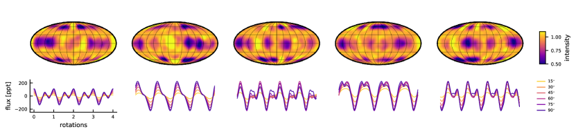
Figure 13: Prior samples from a sum of two starry_process models. The first model consists of small ($r=10^{\circ}$) circumpolar ($\phi=60^{\circ}\pm 3^{\circ}$) spots and the second model consists of larger ($r=20^{\circ}$) equatorial ($\phi=0^{\circ}\pm 3^{\circ}$) spots. The sum of two starry_process models is also a starry_process, making it easy to model more complex distributions of spots.   

Fortunately, Gaussian distributions (and thus also Gaussian processes) are closed under addition, meaning that the sum of two GPs is also a GP. We can thus construct more complex models for stellar variability by summing GPs with different spot hyperparameter vectors $\boldsymbol{\theta}_{\bullet}$. The composite GP will then have a mean equal to the sum of the means of each GP, and a covariance matrix equal to the sum of the covariance matrices of each GP. One possible application of this is to model stars with multiple active latitudes, as described above; an example of this is shown in Figure 13, where samples are drawn from a GP with small circumpolar spots and large equatorial spots (see caption for details). Since the composite GP inherits all of the properties of the standard GP, it can be used to do inference under more complex priors than those presented here.

It is also worth noting that this technique may be employed to model arbitrary distributions for parameters like the spot radius and the number of spots. In the Appendix we present a formulation of our GP that admits a radius distribution half-width parameter $\Delta r$; this generalizes our delta function distribution to a uniform distribution between $r-\Delta r$ and $r+\Delta r$. One may then compute the weighted sum of several GPs with half-widths $\Delta\neq 0$ and central radii $r=r_{0}$, $r=r_{0}+2\Delta r$, $r=r_{0}+4\Delta r$, etc., to approximate any distribution of spot radii. Similarly, one may compute the weighted sum of several GPs with different values of the number of spots $n$ to enforce any discrete distribution for that quantity. The reader should keep in mind that the cost of computing the GP covariance matrix will scale linearly with the number of GP components. In many cases, however, the computational bottleneck is the covariance factorization step (Luger et al., 2021a), in which case adding components to the model will result in negligible overhead.

5.2 Time evolution

Another big limitation of the base algorithm is the implicit assumption that stellar surfaces are static. Our GP hyperparameters $\boldsymbol{\theta}_{\bullet}$ describe the spatial configuration of starspots, but they say nothing about their evolution in time. We know from observations of the Sun and of Kepler stars that temporal variability is extremely common: spots appear, disappear, and even migrate in latitude over time. While it may be possible to parametrize their evolution in a way that is general enough to capture all the ways in which they may change over time, such an approach is beyond the scope of the present paper. It is, however, straightforward to implement an uninformative temporal prior within the framework of our GP. To do this, we will make two simplifying assumptions:

1. The temporal process is stationary. This implies that there is no preferred time (or phase) and that the spatial covariance is the same at all points in time. Stars may still have active longitudes under this assumption, but there is no preferred longitude across all stars.

2. The temporal and spatial covariances are independent. This implies that the evolution of each spherical harmonic mode in time is independent of the evolution of any of the other modes in time.

There is some tension between these assumptions and our knowledge of how stellar surfaces evolve. Assumption (1) excludes surfaces whose total spottiness changes significantly or whose spots migrate in latitude, as both processes change the spatial covariance over time. Assumption (2) ignores the correlation between spherical harmonic modes due to the migration of spots, which requires the coherent evolution of many modes at once. These assumptions likely limit the ability of our GP to model light curves on very long baselines (i.e., on timescales of years) over which stellar activity cycles take place. However, given that the use case of our algorithm is likely to be the analysis of individual quarters of Kepler and individual sectors of TESS data, our assumptions are likely valid in most cases. Analyses of (say) all quarters of Kepler data could process each quarter at a time in a hierarchical framework in which hyperparameters like the mean spot latitude in each quarter are treated as functions of time.

The two assumptions listed above suggest a fairly straightforward form for the GP covariance in spherical harmonics and time:

$$\boldsymbol{\Sigma}_{\mathbf{y}}^{\mathbf{(t)}}=\mathbf{K}\otimes\boldsymbol{\Sigma}_{\mathbf{y}}\hskip 0.0pt,$$ (32)

where $\mathbf{K}$ is a $(K\times K)$ matrix describing the covariance among the $K$ points in time, $\boldsymbol{\Sigma}_{\mathbf{y}}$ is the $(N\times N)$ matrix describing describing the covariance among the $N\equiv(l_{\mathrm{max}}+1)^{2}$ spherical harmonic coefficients (Equation 10), and $\otimes$ denotes the Kronecker product. The quantity $\boldsymbol{\Sigma}_{\mathbf{y}}^{\mathbf{(t)}}$ is the $(NK\times NK)$ temporal-spatial covariance, whose coefficient at index $(Nk+n,Nk^{\prime}+n^{\prime})$ is the covariance between the spherical harmonic coefficient $y_{n}(t_{k})$ and the spherical harmonic coefficient $y_{n^{\prime}}(t_{k^{\prime}})$, where the index $n$ is related to the spherical harmonic indices $l$ and $m$ via Equation (LABEL:eq:n). Finally, because of our assumption of stationarity, the mean of the GP is still constant and equal to the mean of the static process.

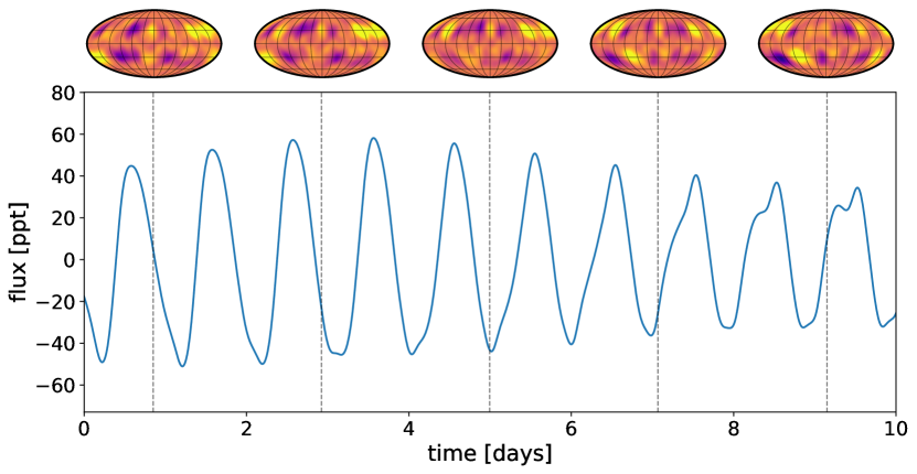
Figure 14: Prior sample from a time-variable starry_process, assuming a rotation period $P=1$ day and a temporal evolution timescale $\tau=20$ days modeled with an exponential squared kernel. Evolving map samples are shown at the top, with the corresponding light curve viewed at an inclination $I=60^{\circ}$ at the bottom. The GP hyperparameters are set to their default values (Table LABEL:tab:synthetic).   

The covariance matrix in Equation (32) can be sampled from to yield time-variable surface maps, or it can be transformed into flux space for sampling light curves or computing likelihoods. The covariance in flux space is given by

$$\boldsymbol{\Sigma}^{\mathbf{(t)}} =\boldsymbol{\mathcal{A}}^{\ddagger}\,\boldsymbol{\Sigma}_{\mathbf{y}}^{\mathbf{(t)}}\,{\boldsymbol{\mathcal{A}}^{\ddagger}}^{\top}$$ (33)

where

(34)

(35)

(36)

is a design matrix constructed by staggering the rows of the standard design matrix $\boldsymbol{\mathcal{A}}$ (see Appendix LABEL:sec:starry:basic). The diagonal structure of $\boldsymbol{\mathcal{A}}^{\ddagger}$ is due to the fact that each snapshot of the surface is only observed at a single phase.

In the temporally-variable version of our GP, the covariance matrix in Equation (33) replaces the standard covariance $\boldsymbol{\Sigma}$; it can similarly be modified (§2.5) to obtain the covariance of the normalized process. While $\boldsymbol{\Sigma}^{\mathbf{(t)}}$ is $(K\times K)$, it is computed from the contraction of a much larger $(NK\times NK)$ matrix, which is extremely inefficient to instantiate and operate on. Fortunately, it can be shown that

$$\boldsymbol{\Sigma}^{\mathbf{(t)}} =\boldsymbol{\mathcal{A}}^{\ddagger}\,\boldsymbol{\Sigma}_{\mathbf{y}}^{\mathbf{(t)}}\,{\boldsymbol{\mathcal{A}}^{\ddagger}}^{\top}$$

$$=\boldsymbol{\mathcal{A}}^{\ddagger}\left(\mathbf{K}\otimes\boldsymbol{\Sigma}_{\mathbf{y}}\right){\boldsymbol{\mathcal{A}}^{\ddagger}}^{\top}$$

$$=\boldsymbol{\Sigma}\odot\mathbf{K}\hskip 0.0pt,$$  (37)

that is, the flux covariance is just the elementwise $\odot$ product of the GP covariance $\boldsymbol{\Sigma}$ and the temporal covariance $\mathbf{K}$. This fact makes the temporal GP just as efficient to evaluate as the standard GP!

Armed with this algorithm for computing $\boldsymbol{\Sigma}^{\mathbf{(t)}}$, it only remains for us to decide on a structure for $\mathbf{K}$. While this can in principle be any covariance matrix constructed from a stationary kernel, we recommend one of the common radial kernels such as the exponential squared kernel

$$k_{\mathrm{E^{2}}}(\Delta t) =\sigma^{2}\exp\left(-\frac{\Delta t^{2}}{2\tau}\right)$$ (38)

or the Matérn-3/2 kernel

$$k_{\mathrm{M^{\frac{3}{2}}}}(\Delta t) =\sigma^{2}\left(1+\frac{\sqrt{3}\Delta t}{\tau}\right)\exp\left(-\frac{\sqrt{3}\Delta t}{\tau}\right)$$ (39)

with variance parameter $\sigma^{2}$ set to unity (since the variance is already specified within $\boldsymbol{\Sigma}$). In this case, the temporal covariance $\mathbf{K}$ is a function of a single parameter: the timescale of the variability, $\tau$. Similar to the other hyperparameters of our GP, this parameter can be estimated in an inference setting. However, a detailed investigation of the ability of our temporal GP to accurately capture spot variability is beyond the scope of this paper, and will be revisited in the future, along with an algorithm to explicitly model the effects of differential rotation on the covariance structure.

Figure 14 shows a single prior sample from the temporal GP described above, assuming a squared exponential covariance with $\tau=20$ days and a rotation period $P=1$ day. We compute both the map samples at five different times (top) and the light curve sample over ten rotations (bottom). The flux variability is qualitatively similar to that seen in temporally-variable Kepler light curves.

5.3 Marginalizing over period and limb darkening

In §2.4 we discussed the value of marginalizing over the stellar inclination when computing the GP covariance (and thus the likelihood). When jointly analyzing the light curves of many stars (which we have repeatedly argued is the best way to infer their spot properties), it can be extremely useful to minimize the number of latent variables associated with individual stars by analytically marginalizing over them. This can dramatically reduce the number of free parameters, turning a difficult inference problem in (possibly) hundreds or thousands of dimensions into a much easier problem in a handful of dimensions. We showed how it is possible to marginalize away the dependence of our GP on the inclinations of individual stars, which is a huge step in this direction. However, our GP remains a function of two other quantities that will in general be different for different stars: the stellar rotation period $P$ and the limb darkening coefficient vector $\mathbf{u}$. We argued that in some cases one may be able to fix the period of each star at an estimate obtained in a pre-processing step (i.e., from a periodogram) and fix the limb darkening coefficients at theoretical values, in which case the number of free parameters of the GP is equal to the size of the spot hyperparameter vector $\boldsymbol{\theta}_{\bullet}$ (five by default), and independent of the number of light curves in the ensemble. However, this procedure ignores any uncertainty in the period and limb darkening coefficients, which could be significant; it is also subject to bias due to the fact that there may be systematic errors in theoretical models for the limb darkening coefficients, particularly for low mass stars (e.g., Kervella et al., 2017). A much better approach would be to analytically marginalize over these two quantities.

Consider Equation (LABEL:eq:akT) in the Appendix, from which the rows of the design matrix (which transforms vectors in the spherical harmonic basis to vectors representing the flux at a point in time) are computed. Marginalization over the inclination, which we demonstrated how to perform analytically in Appendix LABEL:sec:inc, entails integrating over the term $\mathbf{R}_{\hat{\mathbf{x}}}\left(-I\right)$, the Wigner matrix that rotates the star by the inclination angle $I$ into the observer’s frame. Similarly, marginalization over the rotation period would entail integration over the term $\mathbf{R}_{\hat{\mathbf{z}}}\left(\frac{2\pi}{P}t_{k}\right)$, another Wigner matrix that rotates the star to the correct rotational phase at time $t=t_{k}$. Given an appropriate prior on the rotational angular frequency $\frac{2\pi}{P}$, it should be possible to follow the same procedure outlined in Appendix LABEL:sec:inc to analytically compute the first two moments of the distribution of light curves marginalized over the rotation period.

Equation (LABEL:eq:akT) also makes clear the dependence of the GP on the limb darkening cofficients, which enter via the limb darkening operator $\mathbf{L}(\mathbf{u})$. The coefficients of this matrix are linear in the limb darkening coefficients $u_{1}$ and $u_{2}$ (see Equation LABEL:eq:ld:L), so it should be possible to derive closed form solutions to the relevant integrals over $\mathbf{L}(\mathbf{u})$ to yield the GP covariance marginalized over $\mathbf{u}$. It may be possible to compute the marginalized covariance even when parametrizing the quadratic limb darkening coefficients in terms of the uncorrelated $q_{1}$ and $q_{2}$ parameters from Kipping (2013), which would allow us to incorporate hard constraints on positivity and strict limb darkening (as opposed to brightening) directly into the prior.

Given the complexity of the operations involved, performing these marginalizations is beyond the scope of the present paper. However, given the significant computational benefits of this marginalization, as well as the fact that the mapping problem is particularly sensitive to the limb darkening coefficients (Paper I), marginalizing over $P$ and $\mathbf{u}$ will be the subject of an upcoming paper.

5.4 Modeling transits and radial velocity datasets

Finally, we would like to note that the GP developed in this paper is not limited to modeling rotational light curves of stars. We derived the covariance structure of spotted stellar surfaces in the spherical harmonic basis, which we then linearly transformed into flux space to obtain the light curve GP presented above. However, our GP may be used to model any kind of observation that is linearly related to the spherical harmonic representation. If $\mathbf{A}$ is the linear operator that transforms the spherical harmonic representation $\mathbf{y}$ to the data vector $\mathbf{d}$ via $\mathbf{d}=\mathbf{A}\mathbf{y}$, then the mean and covariance of the GP model for $\mathbf{d}$ are given by

$$\boldsymbol{\mu}_{\mathbf{d}} =\mathbf{A}\,\boldsymbol{\mu}_{\mathbf{y}}$$ (40)

$$\boldsymbol{\Sigma}_{\mathbf{d}} =\mathbf{A}\,\boldsymbol{\Sigma}_{\mathbf{y}}\,\mathbf{A}^{\top}\hskip 0.0pt,$$ (41)

respectively, where $\boldsymbol{\mu}_{\mathbf{y}}$ and $\boldsymbol{\Sigma}_{\mathbf{y}}$ are the mean and covariance in the spherical harmonic basis derived in this paper. In Luger et al. (2019) we showed that occultation light curves are also linearly related to the spherical harmonic representation of the stellar surface, so it is straightforward to use our GP to model transits of planets across spotted stars, either to marginalize over the spot variability or to constrain the surface map of the star. In this context, $\mathbf{A}$ may be computed via the design_matrix() method of a Map instance of the starry package.

The formalism developed here may also be extended to model radial velocity (RV) datasets, although this requires a bit more work. The instantaneous radial velocity shift $v$ induced by a rotating spotted star may be approximated as

$$v =\frac{\iint_{S}I\,V\,\mathrm{d}S}{\iint_{S}I\mathrm{d}S}$$ (42)

where $I$ is the stellar intensity at a point on the surface, $V$ is the radial component of the rotational velocity vector at that point, and the integral is taken over the projected disk of the star. If we expand the surface intensity distribution in spherical harmonics, the integral in the denominator is just a classical starry integral, as it is just the disk-integrated intensity (i.e., the flux). The numerator may also be computed following the starry formalism, provided we weight the surface intensity representation by the velocity field $V$. In the case of rigid body rotation, $V$ is exactly a dipole ($l=1$) field, so the quantity $IV$ can be expressed exactly as a product of spherical harmonics. Since spherical harmonics are closed under multiplication, we may write $IV$ as a linear combination of spherical harmonics, meaning the integral in the numerator is also a starry integral. For some linear operators $\mathbf{A}$ and $\mathbf{B}$, we may therefore write

$$\mathbbb{v} =\frac{\mathbf{B}\,\mathbbb{y}}{\mathbf{A}\,\mathbbb{y}}$$ (43)

where $\mathbbb{v}$ is the random variable representing the observed radial velocity time series, $\mathbbb{y}$ is the Gaussian random variable representing the spherical harmonic coefficients describing the stellar surface, and the division is performed elementwise. Since $\mathbbb{v}$ is the ratio of two Gaussian random variables, its distribution is not Gaussian. However, we can still compute the first two moments of the distribution of $\mathbbb{v}$ to derive a Gaussian approximation to it (similar to what we did in §2.5), which will yield the mean and covariance of the Gaussian process representation of the radial velocity time series. Given the complexity of the operations described above, we defer this calculation (and the calibration of the resulting GP model) to future work.

6 Conclusions

This paper is the second in a series devoted to the development of statistically rigorous techniques to model stellar surfaces based on unresolved photometric and spectroscopic measurements. Here, we presented a new Gaussian process (GP) model for stellar variability whose hyperparameters explicitly correspond to physical properties of the stellar surface. Our GP allows one to efficiently compute the likelihood function for stellar light curves marginalized over nuisance parameters such as the specific sizes, positions, and contrasts of individual spots, which are generally unknowable due to the extreme degeneracies involved in the light curve mapping problem. Our GP therefore makes it easy to do posterior inference on the real quantities of interest: parameters controlling the distribution of spot sizes, latitudes, and contrasts within a star and/or across many stars in an ensemble.

Because our expression for the GP covariance has an exact, closed-form solution as a function of the spot parameters, it can be computed efficiently: a typical likelihood evaluation on a dataset consisting of $K\sim 1{,}000$ points takes about 20ms on a modern laptop. Our algorithm is implemented in the open-source, user-friendly Python package starry_process, which is pip-installable, available on GitHub, and described in Luger et al. (2021a). The algorithm is implemented in a combination of C++ and Python, linked using the theano package. Because our GP covariance has an exact representation, so too do its derivatives. We therefore implement backpropagated derivatives with respect to all input parameters for out-of-the-box usage with gradient-based inference and optimization tools such as Hamiltionain Monte Carlo (HMC), autodifferentation variational inference (ADVI), and gradient-based nested sampling.

We devoted a large portion of this paper to testing the algorithm on a variety of synthetic datasets, showing that it is a well-calibrated and in most cases unbiased estimator for starspot properties. Below we list our main results:

1. Our GP works best for ensemble analyses. The light curve mapping problem is extremely degenerate, as light curves contain a vanishingly small fraction of the total information about a stellar surface. However, the degenerate surface modes are a strong function of the observer’s viewing angle, so light curves of stars seen at different inclinations constrain different components of the surface. We have shown that if we jointly analyze the light curves of many stars, we can break many of the degeneracies at play and uniquely infer the statistical properties of the spots across the ensemble. This type of analysis works best if the stars in the ensemble are statistically similar: i.e., the properties of their spots are all drawn from the same parent distribution, whose parameters we can constrain.

2. Typically, an ensemble of at least $M\sim 50$ light curves is needed to place meaningful constraints on starspot properties. This estimate is based on ensemble analyses of light curves with $K=1{,}000$ cadence each and per-cadence precision of one part per thousand. Lower quality, shorter baseline observations, or datasets contaminated by outliers will in general require larger values of $M$ for the same constraining power. The presence of strong limb darkening also degrades the information content of light curves, in which case an ensemble of hundreds or even a thousand light curves is recommended.

3. Our GP is in most cases an unbiased estimator for the spot radius and latitude distributions. We showed that our GP can accurately infer the angular size of spots and the mode and standard deviation of their distribution in latitude from stellar light curves. For the fiducial ensemble of $M=50$ light curves described above, we are able to constrain the average spot radii to within a couple degrees and the average spot latitudes to within $5^{\circ}$.

4. Our GP can accurately infer stellar inclinations. We presented two versions of our GP: one conditioned on a specific value of the stellar inclination, and one marginalized over inclination under an isotropic prior. In both cases, we find that we can accurately infer the inclinations of individual stars in an ensemble analysis (in the latter case, a simple post-processing step can yield the inclination posterior distribution). While the inclination is not an observable for an individual stellar light curve, the population-level constraints on the spot properties achieved by the GP can break the degeneracies involving the inclination, allowing us to usually infer it to within about $10^{\circ}$ and without bias.

5. Our GP can be used to model small, Sun-like spots. The algorithm presented here is limited to a surface resolution of about $10^{\circ}$, corresponding to spots about an order of magnitude larger than typical sunspots. However, we have showed that when we apply our model to light curves of stars with small ($r\sim 3^{\circ}$) spots, we can still infer their latitudinal distribution without bias, as well as the presence of spots below our resolution limit.

6. Our GP can be extended to model time-variable surfaces. The algorithm presented here was derived for static stellar surfaces, corresponding to perfectly periodic light curves. However, time variability can easily be modeled as the product of the starry_process kernel and a kernel describing the covariance of the process in time, such as a simple exponential squared or Matérn-3/2 kernel. The hyperparameters of the temporal covariance are then strictly tied to the timescale on which the surface evolves. More complex temporal variability, such as that induced by differential rotation, will be the subject of a future paper in this series.

7. Our GP can be used in exoplanet transit modeling and radial velocity datasets. At its core, the starry_process GP defines a distribution over spherical harmonic representations of stellar surfaces. It can therefore be used as a physically interpretable prior when modeling transits of exoplanets across spotted stars, either to marginalize over the stellar inhomogeneity or to explicitly infer spot properties. When combined with the starry package, it can also be used as a prior on the stellar surface in Doppler imaging, Doppler tomography, or even radial velocity searches for exoplanets. The latter will be the subject of a future paper in this series.

The GP presented here has far-ranging applications for stellar light curve studies. It serves as a drop-in replacement for commonly used GP kernels for stellar variability, which currently do not have physically interpretable parameters other than the rotation period and, in some cases, a spot evolution timescale. As such, it can be used to marginalize over stellar rotational variability signals in (say) transiting exoplanet searches, asteroseismic characterization of stars, radial velocity searches, etc. It can also be used to learn about stellar surfaces directly: to infer spot properties of main sequence stars as a function of spectral type and age, to differentiate between spot-dominated and plage-dominated stellar surfaces, to better understand chemically peculiar massive stars, and to better understand the spot properties of transiting exoplanet hosts for unbiased spectroscopic characterization of their atmospheres (to name a few).

The next papers in this series will focus on (in no particular order)

• A more rigorous treatment of time variability. This paper will focus on modeling differential rotation, whose effect on the covariance of the process can be derived in a similar fashion to what we did here. This will enable direct inference about the differential rotation rates and spot evolution timescales of stars, processes whose effects on light curves are too similar for current methodology to reliably discern between them.

• Explicit marginalization over the remaining stellar parameters. These include the stellar rotation period and limb darkening coefficients, which can be marginalized over analytically under certain choices of prior. This will eliminate all per-star hyperparameters in the expression for the GP covariance, greatly speeding up inference for large ensembles of stellar light curves.

• Extension of this formalism to radial velocity datasets. As we discussed in §5.4, it is possible to extend the methodology presented here to model the contribution of stellar surface variability to radial velocity measurements, which can be used (for instance) to mitigate systematics in extreme precision radial velocity (EPRV) searches for exoplanets.

• Extension of this formalism to Doppler imaging. As we show in upcoming work, it is possible to derive an exact linear relationship between the wavelength-dependent spherical harmonic representation of a rotating star and its time-variable spectrum. This linearity makes it possible to adapt our GP formalism to the Doppler imaging problem, providing an efficient marginal likelihood function for rigorous inference studies.

In keeping with other papers in the starry series, all figures in this paper are generated automatically from open-source scripts linked to in each of the captions , and the principal equations link to associated unit tests that ensure the accuracy and reproducibility of the algorithm presented here /.

We would like to thank David W. Hogg, Michael Gully-Santiago, Adam Jermyn, Megan Bedell, Will Farr, Dylan Simon, and the Astronomical Data Group at the Center for Computational Astrophysics for their help and for many thought-provoking discussions that made this paper possible.

Table 2: List of common variables and symbols used throughout this paper.

Symbol	Description	Reference
$\mathbf{1}$	Vector of ones	—
$\sim$	Denotes a normalized vector-valued random variable	§2.5
$\odot$	Elementwise product	§5.2
$\otimes$	Kronecker product	§5.2
$a$	GP hyperparameter: spot latitude shape parameter	Appendix LABEL:sec:lat
$\mathbf{a}^{\top}$	Row of the starry design matrix	Equation (LABEL:eq:Arows)
$\mathbf{A_{1}}$	starry change of basis matrix	Appendix LABEL:sec:starry
$\boldsymbol{\mathcal{A}}$	starry design matrix	Equation (LABEL:eq:Arows)
$\alpha$	GP hyperparameter: spot latitude shape parameter	Appendix LABEL:sec:lat
$b$	GP hyperparameter: spot latitude shape parameter	Appendix LABEL:sec:lat
$\beta$	GP hyperparameter: spot latitude shape parameter	Appendix LABEL:sec:lat
$c$	GP hyperparameter: spot contrast	Appendix LABEL:sec:contrast
$\mathbb{c}$	Spot contrast (random variable)	Appendix LABEL:sec:contrast
$\Gamma(\cdots)$	Gamma function	—
$\mathbf{D}_{\mathbf{u}}$	Complex Wigner rotation matrix about an axis $\mathbf{u}$	Appendix LABEL:sec:wigner
$\delta(\cdots)$	Delta function	—
$\delta_{ij}$	Kronecker delta	—
$\Delta r$	GP hyperparameter: spot radius spread	Appendix LABEL:sec:size
$\mathrm{E}\big{[}\cdots\big{]}$	Expected value	Equation (5)
$\mathbf{e}_{I}$	First moment integral of the inclination	Equation (20)
$\mathbf{e}_{r}$	First moment integral of the radius	Equation (LABEL:eq:e1)
$\mathbf{e}_{\phi}$	First moment integral of the latitude	Equation (LABEL:eq:e2)
$\mathbf{e}_{\lambda}$	First moment integral of the longitude	Equation (LABEL:eq:e3)
$\mathbf{e}_{c}$	First moment integral of the contrast	Equation (LABEL:eq:e4)
$\mathbf{E}_{I}$	Second moment integral of the inclination	Equation (21)
$\mathbf{E}_{r}$	Second moment integral of the radius	Equation (LABEL:eq:E1)
$\mathbf{E}_{\phi}$	Second moment integral of the latitude	Equation (LABEL:eq:E2)
$\mathbf{E}_{\lambda}$	Second moment integral of the longitude	Equation (LABEL:eq:E3)
$\mathbf{E}_{c}$	Second moment integral of the contrast	Equation (LABEL:eq:E4)
$\mathbf{f}$	Flux vector	Equation (3)
$\mathbbb{f}$	Flux vector (random variable)	Equation (1)
${{}_{2}}F_{1}(\cdots)$	Gauss hypergeometric function	—
$\boldsymbol{\theta}_{\bullet}$	Vector of GP hyperparameters	Equation (13)
$I$	Stellar inclination	—
$\mathbb{I}$	Stellar inclination (random variable)	§2.4
$J$	Jacobian of the spot latitude transform	Equation (LABEL:eq:J)
$k(\Delta t)$	GP kernel function	Equation (2.1)
$K$	Number of points in light curve	—
$\mathbf{K}$	Temporal covariance matrix	§5.2
$l$	Spherical harmonic degree	Appendix A
$\mathbf{L}$	Limb darkening operator	§LABEL:sec:ld
$\mathcal{L}$	Likelihood function	Equation (2.3)
$\bblambda$	Spot longitude (random variable)	Appendix LABEL:sec:lon
$m$	Spherical harmonic order	Appendix A
$M$	Number of light curves in ensemble	—
$\mu$	Flux GP mean	Equation (2.4)
$\boldsymbol{\mu}$	Flux GP mean vector	Equation (7)
$\boldsymbol{\mu}_{\mathbf{y}}$	Spherical harmonic GP mean vector	Equation (9)
$n$	GP hyperparameter: number of spots	Appendix LABEL:sec:integrals
$\mathbb{n}$	Number of spots contrast (random variable)	Appendix LABEL:sec:integrals
$\mathcal{N}(\mu,\sigma^{2})$	Normal distribution: mean $\mu$, variance $\sigma^{2}$	—
$p(\cdots)$	Probability, probability density	—
$P$	Stellar rotation period	—
$r$	GP hyperparameter: spot radius	Appendix LABEL:sec:size
$\mathbf{r}^{\top}$	Integral over unit disk of polynomial basis	Appendix LABEL:sec:starry
$\mathbb{r}$	Spot radius (random variable)	Appendix LABEL:sec:size
$\mathbf{R}_{\mathbf{u}}$	Real wigner rotation matrix about an axis $\mathbf{u}$	Appendix LABEL:sec:wigner
$\mathbf{s}$	Spherical harmonic expansion of spot	Equation (LABEL:eq:sofr)
$\sigma_{f}$	Photometric uncertainty	§3
$\sigma_{\phi}$	GP hyperparameter: spot latitude standard deviation	Appendix LABEL:sec:lat
$\boldsymbol{\Sigma}$	Flux GP covariance matrix	Equation (8)
$\boldsymbol{\Sigma}^{\mathbf{(t)}}$	Flux GP covariance matrix w/ temporal evolution	Equation (8)
$\tilde{\boldsymbol{\Sigma}}$	Flux GP covariance matrix (normalized processs)	Equation (24)
$\boldsymbol{\Sigma}_{\mathbf{y}}$	Spherical harmonic GP covariance matrix	Equation (10)
$\boldsymbol{\Sigma}_{\mathbf{y}}^{\mathbf{(t)}}$	Spherical harmonic GP covariance w/ temporal evolution	Equation (10)
$t$	time	—
$\tau$	GP hyperparameter: timescale	§5.2
$\mathbf{u}$	Limb darkening coefficient vector	Appendix LABEL:sec:ld
$u_{1},u_{2}$	Linear and quadratic limb darkening coefficients	Appendix LABEL:sec:ld
$\mathbf{U}$	Complex-to-real basis change operator (Wigner matrices)	Appendix LABEL:sec:wigner
$\mathcal{U}(a,b)$	Uniform distribution between $a$ and $b$	—
$\mathbbb{x}$	Random vector of spot properties	Equation (LABEL:eq:x)
$\mathbf{y}$	Spherical harmonic coefficient vector	Equation (3)
$\mathbbb{y}$	Spherical harmonic coefficient vector (random variable)	Equation (LABEL:eq:RRs)
$\mu_{\phi}$	GP hyperparameter: spot latitude mode	Appendix LABEL:sec:lat
$\bbphi$	Spot latitude (random variable)	Appendix LABEL:sec:lat
$z$	GP normalization number	Equation (25)

Appendix A Notation

Unless otherwise noted, we adopt the following conventions throughout this paper: integers are represented by italic uppercase letters (i.e., $K$), scalars are represented by italic lowercase letters (i.e., $x$), column vectors are represented by boldface lowercase letters ($\mathbf{x}$), and matrices are represented by boldface capital letters ($\mathbf{X}$). In general, the elements of a vector $\mathbf{x}$ are denoted $x_{i}$ and the elements of a matrix $\mathbf{X}$ are denoted $X_{i,j}$. Importantly, we make a distinction between quantities like $X_{i,j}$ and $\mathbf{X}_{i,j}$: the former is a scalar element of a matrix, while the latter is a matrix, which is itself a component of a higher-dimensional (in this case, 4-dimensional) linear operator. Thus, lowercase bold symbols always represent vectors, and uppercase bold symbols always represent matrices.

We also make an explicit distinction between numerical quantities and random variables. The former are typeset in serif font (as above), while the latter are typeset in blackboard font. For example, the quantity $\mathbb{x}$ denotes a scalar random variable, while $x$ denotes a particular realization of that variable. The same applies to vector-valued ($\mathbf{x}$ is a realization of $\mathbbb{x}$) and matrix-valued random variables ($\mathbf{X}$ is a realization of $\mathbbb{X}$).

Much of the math in this paper involves vectors representing coefficients in the spherical harmonic basis, which are customarily indexed by two integers $l$ and $m$. We therefore make an exception to our indexing notation for quantities in the spherical harmonic basis: we use two indices to represent a scalar vector element, $x^{l}_{m}$, and four indices to represent a scalar matrix element, $X^{l,l^{\prime}}_{m,m^{\prime}}$. The upper indices corresponds to the spherical harmonic degree, $l\in[0,l_{\mathrm{max}}]$ and $l^{\prime}\in[0,l_{\mathrm{max}}]$, while the lower indices correspond to the spherical harmonic order, $m\in[-l,l]$ and $m^{\prime}\in[-l^{\prime},l^{\prime}]$. Vector elements are arranged in order of increasing $l$ and, within each $l$, in order of increasing $m$. For example, a vector $\mathbf{x}$ representing a quantity in the spherical harmonic basis up to degree $l_{\mathrm{max}}$ has components given by

$$\mathbf{x} =\left(x^{0}_{0}\,\,\,\,\,\,\,\,\,x^{1}_{-1}\,\,\,x^{1}_{0}\,\,\,x^{1}_{1}\,\,\,\,\,\,\,\,\,\cdots\,\,\,\,\,\,\,\,\,x^{l_{\mathrm{max}}}_{-l_{\mathrm{max}}}\cdots\,\,x^{l_{\mathrm{max}}}_{l_{\mathrm{max}}}\,\,\,\right)^{\top}\hskip 0.0pt,$$ (A1)

while a matrix $\mathbf{X}$ in the same basis has components given by Figure S17: Same as Figures 6 and 7, but for mid-latitude spots with $\mu_{\phi}=45^{\circ}$. The radius and latitude parameters are again inferred correctly.   

Figure S18: Same as Figure A, but for high-latitude spots with $\mu_{\phi}=60^{\circ}$. The radius and latitude parameters are again inferred correctly, although the model cannot rule out the presence of polar spots.   

Figure S19: Same as Figure A, but for equatorial spots with $\mu_{\phi}=0^{\circ}$. Even though the model favors a bimodal distribution at low latitudes, the posterior strongly supports the presence of equatorial spots.   

Figure S20: Same as Figure A, but for isotropically-distributed spots. The posterior accurately captures the cosine-like distribution of spot latitudes.   

Figure S21: Same as Figures 6 and 7, but for high contrast ($c=1$) small ($r=3^{\circ}$) spots (significantly lower than the effective resolution of the model). The hatched regions in the posterior plots for the radius ($r<10^{\circ}$) are excluded by the prior, since the model cannot capture features that small. Despite this, the spot latitude distribution is still inferred correctly, although the spot contrast is off by more than $10\sigma$.   

Figure S22: Same as Figures 6 and 7, but for inference based on a single light curve ($M=1$). The constraints on all of the parameters are dramatically weaker.   

Figure S23: Same as Figures 6 and 7, but for inference based on one thousand light curves ($M=1{,}000$). The constraints on the radius and the latitude parameters are dramatically tighter.

References

- Aigrain et al. (2016) Aigrain, S., et al. 2016, MNRAS, 459, 2408
- Ambikasaran et al. (2015) Ambikasaran, S., et al. 2015, IEEE Transactions on Pattern Analysis and Machine Intelligence, 38, 252
- Angus et al. (2018) Angus, R., et al. 2018, MNRAS, 474, 2094
- Angus et al. (2019) —. 2019, AJ, 158, 173
- Barnes et al. (2001) Barnes, S., et al. 2001, ApJ, 548, 1071
- Basri & Shah (2020) Basri, G., & Shah, R. 2020, ApJ, 901, 14
- Beaumont (2019) Beaumont, M. A. 2019, Annual Review of Statistics and Its Application, 6, 379
- Blei et al. (2016) Blei, D. M., et al. 2016, arXiv e-prints, arXiv:1601.00670
- Brewer & Stello (2009) Brewer, B. J., & Stello, D. 2009, MNRAS, 395, 2226
- Cantiello & Braithwaite (2019) Cantiello, M., & Braithwaite, J. 2019, ApJ, 883, 106
- Collado et al. (1989) Collado, J. R. A., et al. 1989, Computer Physics Communications, 52, 323
- Damasso et al. (2019) Damasso, M., et al. 2019, MNRAS, 489, 2555
- Duane et al. (1987) Duane, S., et al. 1987, Physics Letters B, 195, 216
- Feroz et al. (2009) Feroz, F., et al. 2009, MNRAS, 398, 1601
- Foreman-Mackey et al. (2017) Foreman-Mackey, D., et al. 2017, AJ, 154, 220
- Fuller et al. (2015) Fuller, J., et al. 2015, Science, 350, 423
- Gilbertson et al. (2020) Gilbertson, C., et al. 2020, The Astrophysical Journal, 905, 155. https://doi.org/10.3847/1538-4357/abc627
- Gough & Tayler (1966) Gough, D. O., & Tayler, R. J. 1966, Monthly Notices of the Royal Astronomical Society, 133, 85. https://doi.org/10.1093/mnras/133.1.85
- Gully-Santiago et al. (2017) Gully-Santiago, M. A., et al. 2017, ApJ, 836, 200
- Guo et al. (2018) Guo, Z., et al. 2018, ApJ, 868, 143
- Haywood et al. (2014) Haywood, R. D., et al. 2014, MNRAS, 443, 2517
- Hoffman & Gelman (2011) Hoffman, M. D., & Gelman, A. 2011, arXiv e-prints, arXiv:1111.4246
- Ireland & Browning (2018) Ireland, L. G., & Browning, M. K. 2018, ApJ, 856, 132
- Jones et al. (2017) Jones, D. E., et al. 2017, arXiv e-prints, arXiv:1711.01318
- Kervella et al. (2017) Kervella, P., et al. 2017, A&A, 597, A137
- Kipping (2013) Kipping, D. M. 2013, MNRAS, 435, 2152
- Kucukelbir et al. (2016) Kucukelbir, A., et al. 2016, arXiv e-prints, arXiv:1603.00788
- Luger (2021) Luger, R. 2021, in preparation
- Luger et al. (2019) Luger, R., et al. 2019, AJ, 157, 64
- Luger et al. (2016) —. 2016, AJ, 152, 100
- Luger et al. (2021a) —. 2021a, arXiv e-prints, arXiv:2102.01774
- Luger et al. (2021b) —. 2021b, arXiv e-prints, arXiv:2102.00007
- Luger et al. (2017a) —. 2017a, ApJ, 851, 94
- Luger et al. (2017b) —. 2017b, Nature Astronomy, 1, 0129
- Miesch & Toomre (2009) Miesch, M. S., & Toomre, J. 2009, Annual Review of Fluid Mechanics, 41, 317. https://doi.org/10.1146/annurev.fluid.010908.165215
- Morris (2020a) Morris, B. 2020a, The Journal of Open Source Software, 5, 2103
- Morris (2020b) Morris, B. M. 2020b, ApJ, 893, 67
- Morris et al. (2018) Morris, B. M., et al. 2018, ApJ, 857, 39
- Perger et al. (2020) Perger, M., et al. 2020, arXiv e-prints, arXiv:2012.01862
- Price et al. (2018) Price, L. F., et al. 2018, Journal of Computational and Graphical Statistics, 27, 1
- Rackham et al. (2018) Rackham, B. V., et al. 2018, ApJ, 853, 122
- Rajpaul et al. (2015) Rajpaul, V., et al. 2015, MNRAS, 452, 2269
- Rasmussen & Williams (2005) Rasmussen, C. E., & Williams, C. K. I. 2005, Gaussian Processes for Machine Learning (Adaptive Computation and Machine Learning) (The MIT Press)
- Robertson et al. (2020) Robertson, P., et al. 2020, ApJ, 897, 125
- Schuessler et al. (1996) Schuessler, M., et al. 1996, A&A, 314, 503
- Sikora et al. (2018) Sikora, J., et al. 2018, Monthly Notices of the Royal Astronomical Society, 483, 3127. https://doi.org/10.1093/mnras/sty2895
- Skilling (2004) Skilling, J. 2004, in American Institute of Physics Conference Series, Vol. 735, Bayesian Inference and Maximum Entropy Methods in Science and Engineering: 24th International Workshop on Bayesian Inference and Maximum Entropy Methods in Science and Engineering, ed. R. Fischer, R. Preuss, & U. V. Toussaint, 395–405
- Skilling (2006) Skilling, J. 2006, Bayesian Anal., 1, 833
- Solanki et al. (2006) Solanki, S. K., et al. 2006, Reports on Progress in Physics, 69, 563
- Speagle (2020) Speagle, J. S. 2020, MNRAS, 493, 3132
- Turcotte (2003) Turcotte, S. 2003, in Astronomical Society of the Pacific Conference Series, Vol. 305, Magnetic Fields in O, B and A Stars: Origin and Connection to Pulsation, Rotation and Mass Loss, ed. L. A. Balona, H. F. Henrichs, & R. Medupe, 199
- Vanderburg et al. (2016) Vanderburg, A., et al. 2016, MNRAS, 459, 3565
- Wandelt (2012) Wandelt, B. 2012, Gaussian Random Fields in Cosmostatistics
- Weber & Browning (2016) Weber, M. A., & Browning, M. K. 2016, ApJ, 827, 95
- Wood (2010) Wood, S. N. 2010, Nature, 466, 1102
- Yadav et al. (2015) Yadav, R. K., et al. 2015, A&A, 573, A68