The regularized free fall
I – Index computations

Abstract

Main results are, firstly, a generalization of the Conley-Zehnder index from ODEs to the delay equation at hand and, secondly, the equality of the Morse index and the clockwise normalized Conley-Zehnder index ${\mu^{\rm CZ}}$.

We consider the non-local Lagrangian action functional ${\mathcal{B}}$ discovered by Barutello, Ortega, and Verzini [BOV21] with which they obtained a new regularization of the Kepler problem. Critical points of this functional are regularized periodic solutions $x$ of the Kepler problem. In this article we look at period 1 only and at dimension one (gravitational free fall).

Via a non-local Legendre transform regularized periodic Kepler orbits $x$ can be interpreted as periodic solutions $(x,y)$ of a Hamiltonian delay equation. In particular, regularized $1$-periodic solutions of the free fall are represented variationally in two ways: As critical points $x$ of a non-local Lagrangian action functional and as critical points $(x,y)$ of a non-local Hamiltonian action functional.
As critical points of the Lagrangian action the $1$-periodic solutions have a finite Morse index which we compute first.
As critical points of the Hamiltonian action ${\mathcal{A}}_{\mathcal{H}}$ one encounters the obstacle, due to non-locality, that the $1$-periodic solutions are not generated any more by a flow on the phase space manifold. Hence the usual definition of the Conley-Zehnder index as intersection number with a Maslov cycle is not available. In the local case Hofer, Wysocki, and Zehnder [HWZ95] gave an alternative definition of the Conley-Zehnder index by assigning a winding number to each eigenvalue of the Hessian of ${\mathcal{A}}_{\mathcal{H}}$ at critical points.

In this article we show how to generalize the Conley-Zehnder index to the non-local case at hand. On one side we discover how properties from the local case generalize to this delay equation, and on the other side we see a new phenomenon arising. In contrast to the local case the winding number is not any more monotone as a function of the eigenvalues.

1 Introduction

In celestial mechanics, as well as in the theory of atoms, collisions play an intriguing role. There are many geometric ways how to regularize collisions, see for instance [LC20, Mos70]. In both regularizations, Levi-Civita and Moser, one has to change time. A quite new approach to the regularization of collisions was discovered in the recent article [BOV21] by Barutello, Ortega, and Verzini where the change of time leads to a delayed functional (meaning that the critical point equation is a delay equation). In Section 2 we explain, starting from the physics 1-dimensional Kepler problem, how one arrives at this functional

$$\begin{split}{\mathcal{B}}\colon W^{1,2}_{\times}:=W^{1,2}(\SS^{1},{\mathbb{R}})\setminus\{0\}&\to(0,\infty)\\ x&\mapsto{\color[rgb]{.75,.5,.25}4\left\|x\right\|^{2}}\tfrac{1}{2}\mathopen{\|}x^{\prime}\mathclose{\|}^{2}+\frac{1}{\mathopen{\|}x\mathclose{\|}^{2}}\end{split}$$

where $\mathopen{\|}\cdot\mathclose{\|}$ is the $L^{2}$ norm associated to the $L^{2}$ inner product $\langle\cdot,\cdot\rangle$. One might interpret the functional ${\mathcal{B}}$ as a non-local Lagrangian action functional, a non-local mechanical system, consisting of kinetic minus potential energy

$${\mathcal{B}}(x)=\tfrac{1}{2}\langle x^{\prime},x^{\prime}\rangle_{x}+\frac{1}{\mathopen{\|}x\mathclose{\|}^{2}}$$

Here we use the following metric on the tangent bundle of the loop space

$$\langle\cdot,\cdot\rangle_{x}:={\color[rgb]{.75,.5,.25}4\left\|x\right\|^{2}}\langle\cdot,\cdot\rangle$$

which from the perspective of the manifold is non-local as it depends on the whole loop. Also the potential $x\mapsto-\frac{1}{\mathopen{\|}x\mathclose{\|}^{2}}$ is only defined on the loop space.
The set ${\rm Crit}\,{\mathcal{B}}$ of critical points of the non-local action consists of the smooth solutions $x\in C^{\infty}(\SS^{1},{\mathbb{R}})\setminus\{0\}$ of the second order delay, or non-local, equation

$$x^{\prime\prime}=\alpha x,\qquad\alpha=\alpha_{x}:=\left(\frac{\mathopen{\|}x^{\prime}\mathclose{\|}^{2}}{\mathopen{\|}x\mathclose{\|}^{2}}-\frac{1}{2\mathopen{\|}x\mathclose{\|}^{6}}\right)<0$$ (1.1)

Nevertheless, this non-local Lagrangian action functional admits a Legendre transform which leads to a non-local Hamiltonian that lives on (the $L^{2}$ extension of) the cotangent bundle of the loop space, namely

$$\begin{split}{\mathcal{H}}\colon W^{1,2}_{\times}\times L^{2}&\to{\mathbb{R}}\\ (x,y)&\mapsto\tfrac{1}{2}\langle y,y\rangle^{x}-\frac{1}{\mathopen{\|}x\mathclose{\|}^{2}}\end{split}$$

where we use the dual metric on the cotangent bundle of the loop space

$$\langle\cdot,\cdot\rangle^{x}:={\color[rgb]{.75,.5,.25}\tfrac{1}{4\left\|x\right\|^{2}}}\langle\cdot,\cdot\rangle$$

Associated to the non-local Hamiltonian ${\mathcal{H}}$ there is the non-local Hamiltonian action functional, namely

$$\begin{split}{\mathcal{A}}_{\mathcal{H}}:={\mathcal{A}}_{0}-{\mathcal{H}}\colon W^{1,2}_{\times}\times L^{2}&\to{\mathbb{R}}\\ (x,y)&\mapsto\int_{0}^{1}y(\tau)x^{\prime}(\tau)\,d\tau-{\mathcal{H}}(x,y)\end{split}$$

The natural base point projection and the following injection

$$\pi\colon W^{1,2}_{\times}\times L^{2} \to W^{1,2}_{\times}\qquad \iota\colon W^{1,2}_{\times} \to W^{1,2}_{\times}\times L^{2}$$ (1.2)

$$(x,y) \mapsto x\qquad x \mapsto\left(x,{\color[rgb]{.75,.5,.25}4\mathopen{\|}x\mathclose{\|}^{2}}x^{\prime}\right)$$

are along the sets of critical points inverses of one another – which of course explains the choice of the factor ${\color[rgb]{.75,.5,.25}4\mathopen{\|}x\mathclose{\|}^{2}}$. Therefore the sets

are in one-to-one correspondence. Whereas ${\mathcal{B}}$ at any critical point has a finite dimensional Morse index, in sharp contrast both the Morse index and coindex are infinite at the critical points of ${\mathcal{A}}_{\mathcal{H}}$.

Since the action functional ${\mathcal{A}}_{\mathcal{H}}$ is non-local its critical points cannot be interpreted as fixed points of a flow. Therefore the usual definition of the Conley-Zehnder index as a Maslov index does not make sense. However, in [HWZ95] Hofer, Wysocki, and Zehnder gave a different characterization of the Conley-Zehnder index in terms of winding numbers of the eigenvalues of the Hessian.

We show in this article that this definition of the Conley-Zehnder index makes sense, too, for the critical points of the non-local functional ${\mathcal{A}}_{\mathcal{H}}$. Our main result is equality of Morse and Conley-Zehnder index of corresponding critical points.

Theorem A.

For each critical point $(x,y)$ of ${\mathcal{A}}_{\mathcal{H}}$ the canonical (clockwise normalized) Conley-Zehnder index

$${\mu^{\rm CZ}}(x,y)={\rm Ind}(x)$$

is equal to the Morse index of ${\mathcal{B}}$ at $x$.

Proof.

Proposition 3.7 and Proposition 5.10. ∎

The theorem generalizes the local result, see [Web02], to this non-local case. Note that [Web02, Thm. 1.2] uses the counter-clockwise normalized Conley-Zehnder index ${\mu_{\rm CZ}}=-{\mu^{\rm CZ}}$. Sign conventions are discussed at large in the introduction to [Web17]. The local result was a crucial ingredient in the proof that Floer homology of the cotangent bundle is the homology of the loop space [Vit98, SW06, AS06].

Notation.

We define $\SS^{1}:={\mathbb{R}}/{\mathbb{Z}}$ and consider functions $x\colon\SS^{1}\to{\mathbb{R}}$ as functions defined on ${\mathbb{R}}$ that satisfy $x(\tau+1)=x(\tau)$ for every $\tau\in{\mathbb{R}}$. Throughout $\langle\cdot,\cdot\rangle$ is the standard $L^{2}$ inner product on $L^{2}(\SS^{1},{\mathbb{R}})$ and $\mathopen{\|}\cdot\mathclose{\|}$ is the induced $L^{2}$ norm.

Outlook. Since 2018 first steps have been taken to study Floer homology for delay equations, see [AFS20, AFS19a, AFS19b]. The present article is the first in a series of four dealing with the free fall – the simplest instance which might already exhibit all novelties that occur in comparison to ode Floer homology of the cotangent bundle (which still represents the homology of a space, loop space). The other parts will deal with II “Homology computation via heat flow”, III “Floer homology”, and IV “Floer homology and heat flow homology”.

Acknowledgements. UF acknowledges support by DFG grant FR 2637/2-2.

2 Free gravitational fall

Section 2 is to motivate and explain regularization. Readers familiar with regularization could go directly to subsequent sections.

2.1 Classical

For $r>0$ and $\mathfrak{v}\in{\mathbb{R}}$ let $L(r,\mathfrak{v}):=\frac{1}{2}\mathopen{|}\mathfrak{v}\mathclose{|}^{2}-V(r)$ where $V(r):=-1/r$. Then

$$d_{\mathfrak{v}}L(r,\mathfrak{v})=\mathfrak{v},\qquad d_{r}L(r,\mathfrak{v})=-1/r^{2}$$

Due to the potential one cannot allow $r=0$. Thus the classical action functional

$${\mathcal{S}}_{L}(q):=\int_{0}^{1}L(q(t),\dot{q}(t))\,dt=\int_{0}^{1}\left(\tfrac{1}{2}\left|\dot{q}(t)\right|^{2}+\frac{1}{q(t)}\right)dt$$ (2.3)

is defined on the space

$$W^{1,2}_{+}:=W^{1,2}(\SS^{1},(0,\infty))$$ (2.4)

that consists of absolutely continuous positive functions $q\colon[0,1]\to(0,\infty)$ which are periodic, that is $q(1)=q(0)$, and whose derivative is $L^{2}$ integrable, that is $\mathopen{\|}\dot{q}\mathclose{\|}^{2}:=\int_{0}^{1}\dot{q}(t)^{2}\,dt<\infty$.
The Euler-Lagrange (or critical point) equation is given by the second order ode

$$\frac{d}{dt}d_{2}L(q,\dot{q})=d_{1}L(q,\dot{q})\qquad\Leftrightarrow\qquad\ddot{q}=-\frac{1}{q^{2}}$$ (2.5)

pointwise at $t$. Unfortunately, there are no periodic solutions of this equation. In other words, there are no critical points of ${\mathcal{S}}_{L}$ on the space $W^{1,2}_{+}$, in symbols

$${\rm Crit}\,{\mathcal{S}}_{L}=\emptyset$$ (2.6)

All solutions $q$ with zero initial velocity $v_{0}$ end up in collision with the origin. Set $q_{0}:=q(0)$ and $v_{0}:=\dot{q}(0)$. Multiply (2.5) by $2\dot{q}$ and integrate to get

$$\dot{q}(t)^{2}-v_{0}^{2}=\int_{0}^{t}\underbrace{\ddot{q}2\dot{q}}_{\frac{d}{ds}{\dot{q}}^{2}}ds\stackrel{{\scriptstyle(\ref{eq:EL})}}{{=}}\int_{0}^{t}\underbrace{-\frac{2\dot{q}}{q^{2}}}_{2\frac{d}{ds}{\dot{q}}^{-1}}ds=\frac{2}{q(t)}-\frac{2}{q_{0}}$$

hence

$$\dot{q}(t)=\pm\sqrt{\frac{2}{q(t)}+2E},\qquad E:=\frac{v_{0}^{2}}{2}-\frac{1}{q_{0}}\equiv\frac{\dot{q}(t)^{2}}{2}-\frac{1}{q(t)}$$

This shows that collision and bouncing off happen at infinite velocity. If the particle starts with zero initial velocity, collision happens in finite time since the acceleration $\ddot{q}$ is bounded away from zero.

2.2 Non-local regularization

In this section we explain why Barutello, Ortega, and Verzini [BOV21] discovered their functional ${\mathcal{B}}$ defined on the larger (than $W^{1,2}_{+}$) space

$$W^{1,2}_{\times}:=W^{1,2}_{\times}(\SS^{1},{\mathbb{R}})\setminus\{0\}\quad\supset\quad W^{1,2}(\SS^{1},(0,\infty))=:W^{1,2}_{+}$$

It consists of absolutely continuous maps $x\colon[0,1]\to{\mathbb{R}}$ which are periodic $x(1)=x(0)$, not identically zero $x\not\equiv 0$, and whose weak derivative $x^{\prime}$ is $L^{2}$ integrable.

The key observation is that if on the subset $W^{1,2}_{+}$ – the domain (2.4) of the classical action ${\mathcal{S}}_{L}$ – one defines an operation ${\mathcal{R}}$ that takes the square and appropriately rescales time, then the composition $({\mathcal{S}}_{L}\circ{\mathcal{R}})(x)$ is given by a formula, let’s call it ${\mathcal{B}}(x)$, see Figure 1, that makes perfectly sense on the ambient space $W^{1,2}_{\times}$ whose elements are real-valued and so allow for origin traversing.

Whereas the classical functional ${\mathcal{R}}^{*}{\mathcal{S}}_{L}$ is defined on loops that take values in $(0,\infty)$, thereby not allowing for collisions at $0$, has no critical points, the rescaled functional has critical points when considered on the extended domain $W^{1,2}_{\times}(\SS^{1},{\mathbb{R}})\setminus\{0\}$. These critical points correspond to classical solutions having collisions, that is running into the origin $0$.

Figure 1: Pull-back ${\mathcal{R}}^{*}{\mathcal{S}}_{L}$ gives a formula ${\mathcal{B}}$ that makes sense on a larger space on which critical points exist and represent time rescaled physical trajectories

The key fact is that ${\mathcal{B}}$ admits critical points $x$ on the ambient space $W^{1,2}_{\times}$, see (3.26), in which case $q_{x}:={\mathcal{R}}(x)$ solves by Proposition 2.4 the classical free fall equation (2.5) away from a finite set $T_{x}\subset\SS^{1}$ of collision times.

Time rescaling on the small space $W^{1,2}_{+}$

Pick a loop $x\in W^{1,2}_{+}$, see (2.4). We call the variable of the map $x\colon[0,1]\to(0,\infty)$ the regularized time, usually denoted by $\tau$. Classical time we call the values of the map $t_{x}\colon[0,1]\to[0,1]$ defined by

$$t_{x}(\tau):=\frac{\int_{0}^{\tau}x(s)^{2}\,ds}{\mathopen{\|}x\mathclose{\|}^{2}}$$ (2.7)

Classical time has the following properties

$$t_{x}^{\prime}(\tau)=\frac{x(\tau)^{2}}{\mathopen{\|}x\mathclose{\|}^{2}}>0,\quad t_{x}\in C^{1},\quad t_{rx}=t_{x},\quad t_{x}(0)=0,\quad t_{x}(1)=1$$ (2.8)

for every real $r>0$. Since, moreover, the map $t_{x}\colon[0,1]\to[0,1]$ is strictly increasing, it is a bijection and we denote its inverse by

$$\tau_{x}\colon[0,1]\to[0,1]$$

The inverse $\tau_{x}:={t_{x}}^{-1}$ of classical time inherits the property $\tau_{rx}=\tau_{x}$ $\forall r>0$ and

$$\dot{\tau}_{x}(t)=\frac{1}{t_{x}^{\prime}(\tau_{x}(t))}=\frac{\mathopen{\|}x\mathclose{\|}^{2}}{x(\tau_{x}(t))^{2}},\quad\tau_{x}\in C^{1},\quad\tau_{x}(0)=0,\quad\tau_{x}(1)=1$$ (2.9)

Definition 2.1.

The rescale-square operation is defined by

$${\mathcal{R}}\colon W^{1,2}_{+}\to W^{1,2}_{+},\quad x\mapsto x^{2}\circ\tau_{x}$$

We abbreviate $q_{x}:={\mathcal{R}}(x)$. Note that ${\mathcal{R}}(rx)=r^{2}{\mathcal{R}}(x)$ for $r>0$.

Lemma 2.2 (Well defined bijection).

For $x\in W^{1,2}_{+}$ the image ${\mathcal{R}}(x)$ lies in $W^{1,2}_{+}$, too, and the map ${\mathcal{R}}\colon W^{1,2}_{+}\to W^{1,2}_{+}$ is bijective with inverse (2.11).

Proof.

We must show that both are in $L^{2}$, namely a) $q_{x}(t)=x^{2}(\tau_{x}(t))$ and b)

$$\dot{q}_{x}(t)=2x(\tau_{x}(t))\,x^{\prime}(\tau_{x}(t))\,\dot{\tau}_{x}(t)\stackrel{{\scriptstyle(\ref{eq:inverse})}}{{=}}2\mathopen{\|}x\mathclose{\|}^{2}\,\frac{x^{\prime}(\tau_{x}(t))}{x(\tau_{x}(t))}$$

Use that $x$ is continuous, so $\mathopen{\|}x\mathclose{\|}_{L^{\infty}}<\infty$, to get a)

$$\mathopen{\|}q_{x}\mathclose{\|}^{2}=\int_{0}^{1}x^{4}(\tau_{x}(t))\,dt=\mathopen{\|}x\mathclose{\|}_{L^{\infty}}^{4}<\infty$$

In what follows change the variable to $\sigma:=\tau_{x}(t)$ using (2.9) to get b)

$$\mathopen{\|}\dot{q}_{x}\mathclose{\|}^{2}=\int_{0}^{1}\left(2\mathopen{\|}x\mathclose{\|}^{2}\,\frac{x^{\prime}(\tau_{x}(t))}{x(\tau_{x}(t))}\right)^{2}\frac{x^{2}(\sigma)\,d\sigma}{\mathopen{\|}x\mathclose{\|}^{2}}=4\mathopen{\|}x\mathclose{\|}^{2}\left\langle x^{\prime},x^{\prime}\right\rangle<\infty$$ (2.10)

Here the value is finite since $x$ is of class $W^{1,2}$. This proves that ${\mathcal{R}}(x)\in W^{1,2}_{+}$.

Surjective. Given $q\in W^{1,2}_{+}$, set

$${\mathcal{Q}}(q):=x_{q}:=q^{\frac{1}{2}}\circ\tau_{1/\sqrt{q}}$$ (2.11)

Then for $\tau\in[0,1]$ we obtain

$$t_{x_{q}}(\tau)\stackrel{{\scriptstyle\text{def.}}}{{=}}\frac{\int_{0}^{\tau}{x_{q}}^{2}(\sigma)\,d\sigma}{\int_{0}^{1}{x_{q}}^{2}(\sigma)\,d\sigma}=\frac{\int_{0}^{\tau}q\circ\overbrace{\tau_{1/\sqrt{q}}(\sigma)}^{=:s}\,d\sigma}{\int_{0}^{1}q\circ\tau_{1/\sqrt{q}}(\sigma)\,d\sigma}=\frac{\int_{0}^{\tau_{1/\sqrt{q}}(\tau)}\frac{ds}{\mathopen{\|}1/\sqrt{q}\mathclose{\|}^{2}}}{\int_{0}^{1}\frac{ds}{\mathopen{\|}1/\sqrt{q}\mathclose{\|}^{2}}}=\tau_{1/\sqrt{q}}(\tau)$$

by change of variables. With this result we get that

$$\bigl{(}{\mathcal{R}}\circ\underbrace{{\mathcal{Q}}(q)}_{x_{q}}\bigr{)}(t)\stackrel{{\scriptstyle\text{def. ${\mathcal{R}}$}}}{{=}}x_{q}^{2}\circ\tau_{x_{q}}(t)\stackrel{{\scriptstyle\text{def. $x_{q}^{2}$}}}{{=}}q\circ\underbrace{t_{1/\sqrt{q}}}_{t_{x_{q}}}\circ\underbrace{\tau_{x_{q}}}_{{t_{x_{q}}}^{-1}}(t)=q(t)$$

Injective. For $x\in W^{1,2}_{+}$ set $q_{x}:={\mathcal{R}}(x):=x^{2}\circ\tau_{x}$. Then for $t\in[0,1]$ we get

$$\int_{0}^{t}\frac{1}{q_{x}(s)}\,ds=\int_{0}^{t}\frac{1}{x^{2}\circ\tau_{x}(s)}\,ds=\int_{0}^{\tau_{x}(t)}\frac{1}{x^{2}(\sigma)}\frac{x^{2}(\sigma)\,d\sigma}{\mathopen{\|}x\mathclose{\|}^{2}}=\frac{\tau_{x}(t)}{\mathopen{\|}x\mathclose{\|}^{2}}$$

by change of variables $\sigma=\tau_{x}(s)$ using (2.9). Pick $t=1$ to obtain

$$\int_{0}^{1}\frac{1}{q_{x}(t)}\,dt=\frac{1}{\mathopen{\|}x\mathclose{\|}^{2}}$$ (2.12)

Therefore we get for $t\in[0,1]$ the formula

$$\tau_{x}(t)=\mathopen{\|}x\mathclose{\|}^{2}\int_{0}^{t}\frac{1}{q_{x}(s)}\,ds\stackrel{{\scriptstyle(\ref{eq:1/q^2})}}{{=}}\frac{\int_{0}^{t}\frac{1}{q_{x}(s)}\,ds}{\int_{0}^{1}\frac{1}{q_{x}(s)}\,ds}\stackrel{{\scriptstyle(\ref{eq:class-time-tau})}}{{=:}}t_{1/\sqrt{q_{x}}}(t)$$

With this result we obtain

$$\bigl{(}{\mathcal{Q}}\circ\underbrace{{\mathcal{R}}(x)}_{q_{x}}\bigr{)}(\tau)\stackrel{{\scriptstyle\text{def. ${\mathcal{Q}}$}}}{{=}}\sqrt{q_{x}}\circ\tau_{1/\sqrt{q_{x}}}(\tau)\stackrel{{\scriptstyle\text{def. $q_{x}$}}}{{=}}x\circ\underbrace{\tau_{x}}_{t_{1/\sqrt{q_{x}}}}\circ\underbrace{t_{1/\sqrt{q_{x}}}}_{{\tau_{1/\sqrt{q_{x}}}}^{-1}}(\tau)=x(\tau)$$

∎

Lemma 2.3 (Pull-back yields an extendable formula).

Given $x\in W^{1,2}_{+}$, then

$${\mathcal{S}}_{L}({\mathcal{R}}(x))=\tfrac{1}{2}\langle x^{\prime},x^{\prime}\rangle_{x}+\frac{1}{\mathopen{\|}x\mathclose{\|}^{2}}$$

as illustrated by Figure 1.

Note that in the previous formula $x(\tau)$ may take on the value zero at will, even along intervals, as long as $\mathopen{\|}x\mathclose{\|}\not=0$, i.e. as long as $x$ is not constantly zero.

Proof.

Set $q_{x}:={\mathcal{R}}(x)$. Definition (2.3) of ${\mathcal{S}}_{L}$ tells that

$$\begin{split}{\mathcal{S}}_{L}(q_{x})\stackrel{{\scriptstyle(\ref{eq:class-action})}}{{=}}\tfrac{1}{2}\mathopen{\|}\dot{q}_{x}\mathclose{\|}^{2}+\int_{0}^{1}\frac{1}{q_{x}(t)}\,dt=\tfrac{1}{2}\,4\mathopen{\|}x\mathclose{\|}^{2}\left\langle x^{\prime},x^{\prime}\right\rangle+\frac{1}{\mathopen{\|}x\mathclose{\|}^{2}}\end{split}$$ (2.13)

where in the second equality we used (2.10) and (2.12). ∎

2.3 Correspondence of solutions

Whereas the classical action ${\mathcal{S}}_{L}$ does not admit, see (2.6), on the small space $W^{1,2}_{+}$ any critical points, that is no $1$-periodic free fall solutions, the formula (2.13) for ${\mathcal{S}}_{L}$ evaluated on the regularization $q_{x}:={\mathcal{R}}(x)$ of a loop $x\in W^{1,2}_{+}$ makes perfectly sense on the larger Sobolev Hilbert space $W^{1,2}_{\times}:=W^{1,2}(\SS^{1},{\mathbb{R}})\setminus\{0\}$ with the origin removed. This way one arrives, in case of the free fall, at the Barutello-Ortega-Verzini [BOV21] non-local functional

$$\begin{split}{\mathcal{B}}\colon W^{1,2}_{\times}:=W^{1,2}(\SS^{1},{\mathbb{R}})\setminus\{0\}\to(0,\infty),\quad x\mapsto\tfrac{1}{2}\left\langle x^{\prime},x^{\prime}\right\rangle_{x}+\frac{1}{\mathopen{\|}x\mathclose{\|}^{2}}\end{split}$$ (2.14)

For this functional ${\mathcal{B}}$ eventual zeroes of $x$ cause no problem at all. It has even lots of critical points - one circle worth of critical points for each natural number $k\in{\mathbb{N}}$, see Lemma 3.3.

But are the critical points $x\colon\SS^{1}\to{\mathbb{R}}$ of ${\mathcal{B}}$ related to free fall solutions $q\colon{\rm dom\,}q\to(0,\infty)$? If so what is the domain of $q$? Next we prepare to give the answers in Proposition 2.4 below. From now on

• we only consider critical points $x\in W^{1,2}_{\times}$ of ${\mathcal{B}}$ and

• we identify $\SS^{1}$ with $[0,1]/\{0,1\}$.

A priori such $x\colon[0,1]\to{\mathbb{R}}$ might have zeroes and these might obstruct bijectivity of the classical time $t_{x}$ defined as before in (2.7). Indeed the derivative $t_{x}^{\prime}(\tau)=x(\tau)^{2}/\mathopen{\|}x\mathclose{\|}^{2}\geq 0$, more properties in (2.8), might now be zero at some times – precisely the times of collision of the solution $x$ with the origin. By continuity of the map $x\colon[0,1]\to{\mathbb{R}}$ the zero set $T_{x}:=x^{-1}(0)$ is closed, thus compact. On the other hand, the set is discrete because being a critical point $x\not\equiv 0$ solves a second order delay equation, see Corollary 3.2. We denote the finite set of regularized collision times by

$${\mathcal{T}}_{x}:=\{\tau\in[0,1]\mid x(\tau)=0\}=\{\tau_{1},\dots,\tau_{N}\}$$

Thus $t_{x}\colon[0,1]\to[0,1]$ is still strictly increasing, hence a bijection. We denote the inverse again by $\tau_{x}:={t_{x}}^{-1}$ and the set of classical collision times, this terminology will become clear in a moment, by $T_{q_{x}}:=t_{x}({\mathcal{T}}_{x})$, that is

$$T_{q_{x}}:=\{t_{1},\dots,t_{N}\},\quad t_{i}:=t_{x}(\tau_{i})$$

The derivative of $\tau_{x}\colon[0,1]\to[0,1]$ is still given by

$$\dot{\tau}_{x}(t)=\frac{\mathopen{\|}x\mathclose{\|}^{2}}{x(\tau_{x}(t))^{2}}$$ (2.15)

but now only at non-collision times $t$, that is $t\in\SS^{1}\setminus T_{q_{x}}$.

The following proposition is a special case of a theorem due to Barutello, Ortega, and Verzini [BOV21].

Proposition 2.4.

Given a critical point $x\in W^{1,2}_{\times}$ of ${\mathcal{B}}$, namely a solution of (1.1), then the rescale-squared map $q=q_{x}:={\mathcal{R}}(x)$ is a physical solution in the sense that $q$ solves the free fall equation at all times

$$\ddot{q}(t)=-\frac{1}{q(t)^{2}},\qquad\forall t\in\SS^{1}\setminus T_{q_{x}}$$

except at the finitely many collision times which form the set $T_{q_{x}}=\{t_{1},\dots,t_{N}\}$.

Think of the critical points $x$ of ${\mathcal{B}}$ as the regularized versions, “the regularizations”, of the physical solutions $q_{x}$. Note that when the regularization $x$ runs through the big mass sitting at the origin the physical solution $q$ bounces back.

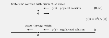
Figure 2: Physical solution $q$ and regularized solution $x$

Proof.

At $t\in\SS^{1}\setminus T_{q_{x}}$, set $\tau(t):=\tau_{x}(t)$, the derivative of $q=q_{x}$ is given by

$$\dot{q}(t)=2\,x(\tau(t))\,x^{\prime}(\tau(t))\underbrace{\dot{\tau}(t)}_{(\ref{eq:t_q^prime})}=2\mathopen{\|}x\mathclose{\|}^{2}\,\frac{x^{\prime}(\tau(t))}{x(\tau(t))}$$ (2.16)

and via a change of variables from $t$ to $s:=\tau(t)$ we get using (2.15) that

$$\mathopen{\|}\dot{q}\mathclose{\|}^{2}={\color[rgb]{.75,.5,.25}4\mathopen{\|}x\mathclose{\|}^{2}}\mathopen{\|}x^{\prime}\mathclose{\|}^{2}\qquad\text{equivalently}\qquad\left\langle\dot{q}_{x},\dot{q}_{x}\right\rangle=\left\langle x^{\prime},x^{\prime}\right\rangle_{x}$$ (2.17)

To calculate the second derivative $\ddot{q}$ use the critical point equation (1.1) to get

$$\begin{split}\ddot{q}(t)&=\frac{2\mathopen{\|}x\mathclose{\|}^{4}}{x(\tau(t))^{3}}\left(x^{\prime\prime}(\tau(t))-\frac{x^{\prime}(\tau(t))^{2}}{x(\tau(t))}\right)\\ &=\frac{1}{q(t)}\left(2\mathopen{\|}x\mathclose{\|}^{2}\mathopen{\|}x^{\prime}\mathclose{\|}^{2}-\frac{1}{\mathopen{\|}x\mathclose{\|}^{2}}\right)-\frac{\dot{q}(t)^{2}}{2q(t)}\\ &=\frac{1}{q(t)}\left(\frac{1}{2}\mathopen{\|}\dot{q}\mathclose{\|}^{2}-\int_{0}^{1}\frac{ds}{q(s)}-\frac{1}{2}\dot{q}(t)^{2}\right)\end{split}$$ (2.18)

To obtain equation three we used the identities (2.17) and (2.12). Let $t_{-},t_{+}\in T_{q_{x}}$ be neighboring collision times in the sense that the interval $(t_{-},t_{+})$ lies in the complement of the collision time set $T_{q_{x}}$.
Similarly to Barutello, Ortega, and Verzini [BOV21, Eq. (3.12)] we consider

$$\beta=\beta_{q}:=\frac{\ddot{q}}{q}$$

as a function on the open non-collision interval $(t_{-},t_{+})$. Differentiate the identity $q^{2}\beta=\left(\frac{1}{2}\mathopen{\|}\dot{q}\mathclose{\|}^{2}-\int_{0}^{1}\frac{dt}{q(t)}-\frac{1}{2}\dot{q}^{2}\right)$ to obtain that $2q\dot{q}\beta+q^{2}\dot{\beta}=-\dot{q}\ddot{q}=-q\dot{q}\beta$ or equivalently $q^{2}\dot{\beta}=-3\beta q\dot{q}$. Hence the logarithmic derivatives satisfy

$$\frac{\dot{\beta}}{\beta}=-\frac{3\dot{q}}{q}$$

and therefore

$$\beta=\frac{\mu}{q^{3}}$$

for some constant $\mu\in{\mathbb{R}}$ that a priori might depend on the interval $(t_{-},t_{+})$. By definition of $\beta$ we conclude that

$$\ddot{q}=\frac{\mu}{q^{2}}$$

on the interval $(t_{-},t_{+})$. By (2.18) we get for the constant $\mu$ the expression

$$\begin{split}\mu&=q(t)\left(\frac{1}{2}\mathopen{\|}\dot{q}\mathclose{\|}^{2}-\int_{0}^{1}\frac{ds}{q(s)}\right)-\frac{1}{2}q(t)\dot{q}(t)^{2}\\ &=q(t)\left(\frac{1}{2}\mathopen{\|}\dot{q}\mathclose{\|}^{2}-\int_{0}^{1}\frac{ds}{q(s)}\right)-2\mathopen{\|}x\mathclose{\|}^{4}x^{\prime}(\tau(t))^{2}\end{split}$$

where in the second equation we used (2.16). Taking the limits $t\to t_{\pm}$ we get

$$\mu=-2\mathopen{\|}x\mathclose{\|}^{4}x^{\prime}(\tau(t_{\pm}))^{2}\leq 0$$

Thus the constant $\mu$ takes the same value on the boundary of adjacent intervals. Hence the constant $\mu$ is independent of the interval.

To see that $\mu=-1$ we multiply (2.18) by $q$ and use $q^{\prime\prime}=\mu/q^{2}$ to obtain

$$\frac{\mu}{q}=\frac{1}{2}\mathopen{\|}\dot{q}\mathclose{\|}^{2}-\int_{0}^{1}\frac{ds}{q(s)}-\frac{1}{2}\dot{q}(t)^{2}$$

We take the mean value of this equation to get that

$$\mu\int_{0}^{1}\frac{dt}{q(t)}=\frac{1}{2}\mathopen{\|}\dot{q}\mathclose{\|}^{2}-\int_{0}^{1}\frac{dt}{q(t)}-\frac{1}{2}\mathopen{\|}\dot{q}\mathclose{\|}^{2}=-\int_{0}^{1}\frac{dt}{q(t)}$$

This shows that $\mu=-1$. ∎

3 Non-local Lagrangian mechanics

3.1 Non-local Lagrangian action ${\mathcal{B}}$ and $L^{2}_{x}$ inner product

In the novel approach [BOV21] to the regularization of collisions discovered recently by Barutello, Ortega, and Verzini the change of time leads to a delayed action functional ${\mathcal{B}}$. Section 2 above explains this for the free fall. The delay, that is the non-local term, is best incorporated into the $L^{2}$ inner product on the loop space. More precisely, we introduce a metric on the following Hilbert space take away the origin, namely

$$W^{1,2}_{\times}:=W^{1,2}\setminus\{0\},\qquad W^{1,2}:=W^{1,2}(\SS^{1},{\mathbb{R}})$$

Given a point $x\in W^{1,2}_{\times}$ and two tangent vectors

$$\xi_{1},\xi_{2}\in T_{x}W^{1,2}_{\times}=W^{1,2}$$

we define the $L^{2}_{x}$ inner product by

$$\langle\xi_{1},\xi_{2}\rangle_{x}:={\color[rgb]{.75,.5,.25}4\mathopen{\|}x\mathclose{\|}^{2}}\langle\xi_{1},\xi_{2}\rangle,\qquad\text{where $\langle\xi_{1},\xi_{2}\rangle:=\int_{0}^{1}\xi_{1}(\tau)\xi_{2}(\tau)\,d\tau$}$$ (3.19)

where $\mathopen{\|}x\mathclose{\|}:=\sqrt{\langle x,x\rangle}$ is the $L^{2}$ norm associated to the $L^{2}$ inner product. In our case of the 1-dimensional Kepler problem the functional then attains the form

$$\begin{split}{\mathcal{B}}\colon W^{1,2}_{\times}:=W^{1,2}(\SS^{1},{\mathbb{R}})\setminus\{0\}\to(0,\infty),\quad x\mapsto\tfrac{1}{2}\left\langle x^{\prime},x^{\prime}\right\rangle_{x}+\frac{1}{\mathopen{\|}x\mathclose{\|}^{2}}\end{split}$$

One might interpret this functional as a non-local mechanical system consisting of kinetic minus potential energy.

3.2 Critical points and Hessian operator

Straightforward calculation provides

Lemma 3.1 (Differential of ${\mathcal{B}}$).

The differential $d{\mathcal{B}}\colon W^{1,2}_{\times}\times W^{1,2}\to{\mathbb{R}}$ is

$$\begin{split}d{\mathcal{B}}(x,\xi)&=4\langle x,\xi\rangle\mathopen{\|}x^{\prime}\mathclose{\|}^{2}+4\mathopen{\|}x\mathclose{\|}^{2}\langle x^{\prime},\xi^{\prime}\rangle-2\frac{\langle x,\xi\rangle}{\mathopen{\|}x\mathclose{\|}^{4}}\\ &=-\langle x^{\prime\prime},\xi\rangle_{x}+\underbrace{\left(\frac{\mathopen{\|}x^{\prime}\mathclose{\|}^{2}}{\mathopen{\|}x\mathclose{\|}^{2}}-\frac{1}{2\mathopen{\|}x\mathclose{\|}^{6}}\right)}_{=:\alpha<0}\langle x,\xi\rangle_{x}\end{split}$$

where identity two is valid whenever $x$ is of better regularity $W^{2,2}(\SS^{1},{\mathbb{R}})\setminus\{0\}$.

Note that $\alpha=\alpha_{x}<0$. Indeed $\alpha>0$ is impossible by the periodicity requirement for solutions and $\alpha=0$ is impossible, because otherwise $x$ would vanish identically which is excluded by assumption.

Corollary 3.2 (${\rm Crit}\,{\mathcal{B}}$).

The set of critical points consists of the smooth solutions $x\in C^{\infty}(\SS^{1},{\mathbb{R}})\setminus\{0\}$ of the second order delay equation $x^{\prime\prime}=\alpha x$, see (1.1).

By Lemma 3.1 the $L^{2}_{x}$ gradient of ${\mathcal{B}}$ at a loop $x\in W^{2,2}_{\times}$ is given by

$${\mathop{\mathrm{grad}}}^{x}{\mathcal{B}}(x)=-x^{\prime\prime}+\alpha x,\qquad x\in W^{2,2}_{\times}:=W^{2,2}(\SS^{1},{\mathbb{R}})\setminus\{0\}$$ (3.20)

Solutions of the critical point equation

To find the solutions $x:\SS^{1}\to{\mathbb{R}}$ of equation (1.1) we set $\beta:=-\alpha>0$ to get the second order ode and its solution

$$x^{\prime\prime}=-\beta x,\qquad x(\tau)=C\cos\sqrt{\beta}\tau+D\sin\sqrt{\beta}\tau$$

where $C$ and $D$ are constants. Thus

$$x^{\prime}=-C\sqrt{\beta}\sin\sqrt{\beta}\tau+D\sqrt{\beta}\cos\sqrt{\beta}\tau$$

Since our solutions $x$ is periodic with period $1$ we must have

$$\sqrt{\beta}=2\pi k,\quad k\in{\mathbb{N}}$$ (3.21)

Thus

$$x(\tau)=C\cos 2\pi k\tau+D\sin 2\pi k\tau$$

and

$$x^{\prime}(\tau)=-2\pi kC\sin 2\pi k\tau+2\pi kD\cos 2\pi k\tau$$

Note that integrating the identity $1=\cos^{2}+\sin^{2}$ we get

$$1=\int_{0}^{1}1\,d\tau=\int_{0}^{1}\cos^{2}\,d\tau+\int_{0}^{1}\sin^{2}\,d\tau=2\int_{0}^{1}\cos^{2}(2\pi k\tau)\,d\tau$$ (3.22)

as is well known from the theory of Fourier series. Moreover, from the theory of Fourier series it is known that cosine is orthogonal to sine, that is

$$0=\int_{0}^{1}\cos(2\pi k\tau)\sin(2\pi k\tau)\,d\tau$$

Therefore $\mathopen{\|}x\mathclose{\|}^{2}=\frac{C^{2}+D^{2}}{2}$ and $\mathopen{\|}x^{\prime}\mathclose{\|}^{2}=\frac{C^{2}+D^{2}}{2}\left(2\pi k\right)^{2}$ and so we get that

$$(2\pi k)^{2}\stackrel{{\scriptstyle(\ref{eq:ab-heat})}}{{=}}\beta^{2}\stackrel{{\scriptstyle(\ref{eq:Crit-Lag})}}{{=}}\frac{1}{2\mathopen{\|}x\mathclose{\|}^{6}}-\frac{\mathopen{\|}x^{\prime}\mathclose{\|}^{2}}{\mathopen{\|}x\mathclose{\|}^{2}}=\frac{4}{(C^{2}+D^{2})^{3}}-(2\pi k)^{2},\quad k\in{\mathbb{N}}$$ (3.23)

We fix the parametrization of our solution by requiring that at time zero the solution is maximal. Therefore $D=0$ and we abbreviate $c_{k}:=C(k)>0$. Then $c_{k}$ is uniquely determined by $k$ via the above equation which becomes

$$\frac{4}{c_{k}^{6}}=8\pi^{2}k^{2},\qquad\frac{1}{c_{k}^{6}}=2(\pi k)^{2}$$ (3.24)

Hence

$$c_{k}=\frac{1}{2^{\frac{1}{6}}(\pi k)^{\frac{1}{3}}}\in(0,1),\qquad c_{k}^{2}=\frac{1}{2^{\frac{1}{3}}(\pi k)^{\frac{2}{3}}}$$ (3.25)

Note that $c_{k}<1$. This proves

Lemma 3.3 (Critical points of ${\mathcal{B}}$).

The maps

$$x_{k}(\tau)=c_{k}\cos 2\pi k\tau,\qquad k\in{\mathbb{N}}$$ (3.26)

are solutions of (1.1). Each map $x_{k}$ is worth a circle of solutions via time shift $\sigma_{*}x_{k}:=x_{k}(\cdot+\sigma)$ where $\sigma\in\SS^{1}$. All solutions of (1.1) are given by

$${\rm Crit}\,{\mathcal{B}}=\bigcup_{k\in{\mathbb{N}}}\{\sigma_{*}x_{k}\mid\sigma\in\SS^{1}\}$$

The Hessian operator with respect to the $L^{2}_{x}$ inner product

The Hessian operator $A_{x}$ of the Lagrange functional ${\mathcal{B}}$ is the derivative of the $L^{2}_{x}$ gradient equation $0=-x^{\prime\prime}+\alpha x$ at a critical point $x$. Varying this equation with respect to $x$ in direction $\xi$ we obtain that

$$\begin{split}A_{x}\xi&=-\ddot{\xi}+\alpha\xi+\left(-\frac{2\langle x^{\prime\prime},\xi\rangle}{\mathopen{\|}x\mathclose{\|}^{2}}-\frac{2\mathopen{\|}x^{\prime}\mathclose{\|}^{2}\langle x,\xi\rangle}{\mathopen{\|}x\mathclose{\|}^{4}}+\frac{3\langle x,\xi\rangle}{\mathopen{\|}x\mathclose{\|}^{8}}\right)x\\ &=-\ddot{\xi}+\alpha\xi-\left(\frac{2\alpha}{\mathopen{\|}x\mathclose{\|}^{2}}+\frac{2\mathopen{\|}x^{\prime}\mathclose{\|}^{2}}{\mathopen{\|}x\mathclose{\|}^{4}}-\frac{3}{\mathopen{\|}x\mathclose{\|}^{8}}\right)\left\langle x,\xi\right\rangle x\\ &=-\ddot{\xi}+\alpha\xi-\frac{2}{\mathopen{\|}x\mathclose{\|}^{2}}\left(2\alpha-\frac{1}{\mathopen{\|}x\mathclose{\|}^{6}}\right)\left\langle x,\xi\right\rangle x\end{split}$$

where in step 2 we used the critical point equation $x^{\prime\prime}=\alpha x$ and in step 3 we replaced $2\mathopen{\|}x^{\prime}\mathclose{\|}^{2}$ by $2\alpha\mathopen{\|}x\mathclose{\|}^{2}+\frac{1}{\mathopen{\|}x\mathclose{\|}^{4}}$ according to the definition of $\alpha$. This proves

Lemma 3.4.

The Hessian operator of ${\mathcal{B}}$ at a critical point $x$ is given by

$$\begin{split}A_{x}\colon W^{2,2}(\SS^{1},{\mathbb{R}})&\to L^{2}(\SS^{1},{\mathbb{R}})\\ \xi&\mapsto-\ddot{\xi}+\alpha\xi-\frac{2}{\mathopen{\|}x\mathclose{\|}^{2}}\left(2\alpha-\frac{1}{\mathopen{\|}x\mathclose{\|}^{6}}\right)\left\langle x,\xi\right\rangle x\end{split}$$

Recall that by (3.26) the critical points of ${\mathcal{B}}$ are of the form

$$x_{k}(\tau)=c_{k}\cos 2\pi k\tau,\qquad k\in{\mathbb{N}}$$ (3.27)

with $c_{k}$ given by (3.25). Taking two $\tau$ derivatives we conclude that

$$x^{\prime\prime}_{k}=-(2\pi k)^{2}x_{k}$$

Since $x^{\prime\prime}_{k}=\alpha x_{k}$ we obtain

$$\alpha=\alpha({x_{k}})=-(2\pi k)^{2}=-\frac{2}{c_{k}^{6}}$$

where the last equality is (3.24). The formula of the Hessian operator $A_{x_{k}}$ involves the $L^{2}$ norm of $x_{k}$ and, in addition, the formula of the non-local Lagrange functional ${\mathcal{B}}$ involves $\mathopen{\|}x^{\prime}_{k}\mathclose{\|}^{2}$. By (3.26) and (3.22) we obtain that

$$\left\|x_{k}\right\|^{2}=\frac{c_{k}^{2}}{2}=\frac{1}{2^{\frac{4}{3}}(\pi k)^{\frac{2}{3}}},\qquad\left\|x^{\prime}_{k}\right\|^{2}=(2\pi k)^{2}\frac{c_{k}^{2}}{2}=2^{\frac{2}{3}}(\pi k)^{\frac{4}{3}}$$

Thus

$${\mathcal{B}}(x_{k})=2\mathopen{\|}x_{k}\mathclose{\|}^{2}\mathopen{\|}x^{\prime}_{k}\mathclose{\|}^{2}+\frac{1}{\mathopen{\|}x_{k}\mathclose{\|}^{2}}=2^{\frac{1}{3}}3(\pi k)^{\frac{2}{3}}$$

To calculate the formula of $A_{x_{k}}$ we write $\xi$ as a Fourier series

$$\xi=\xi_{0}+\sum_{n=1}^{\infty}\left(\xi_{n}\cos 2\pi n\tau+\xi^{n}\sin 2\pi n\tau\right)$$

and we use the orthogonality relation

$$\langle\cos 2\pi n\cdot,\xi\rangle=\frac{1}{2}\xi_{n}$$

to calculate the product

$$\langle x_{k},\xi\rangle=\tfrac{1}{2}c_{k}\xi_{k}$$

Putting everything together we obtain

Lemma 3.5 (Critical values and Hessian).

The critical points of ${\mathcal{B}}$ are of the form $x_{k}(\tau)=c_{k}\cos 2\pi k\tau$ for $k\in{\mathbb{N}}$, see (3.27). At any such $x_{k}$ the value of ${\mathcal{B}}$ is

$${\mathcal{B}}(x_{k})=2^{\frac{1}{3}}3(\pi k)^{\frac{2}{3}}$$

and the Hessian operator of ${\mathcal{B}}$ is

$$\begin{split}A_{x_{k}}\xi=-\ddot{\xi}-(2\pi k)^{2}\xi+{\color[rgb]{.75,.5,.25}12(2\pi k)^{2}\xi_{k}}\cos 2\pi k\tau\end{split}$$

for every $\xi\in W^{2,2}(\SS^{1},{\mathbb{R}})$.

3.3 Eigenvalue problem and Morse index

Recall that $k\in{\mathbb{N}}$ is fixed since we consider the critical point $x_{k}$. We are looking for solutions of the eigenvalue problem

$$A_{x_{k}}\xi=\mu\xi$$

for $\mu=\mu(\xi;k)\in{\mathbb{R}}$ and $\xi\in W^{2,2}(\SS^{1},{\mathbb{R}})\setminus\{0\}$. Observe that

$$\begin{split}-\ddot{\xi}&=\sum_{n=1}^{\infty}(2\pi n)^{2}\left(\xi_{n}\cos 2\pi n\tau+\xi^{n}\sin 2\pi n\tau\right)\\ -(2\pi k)^{2}\xi&=-(2\pi k)^{2}\xi_{0}-(2\pi k)^{2}\sum_{n=1}^{\infty}\left(\xi_{n}\cos 2\pi n\tau+\xi^{n}\sin 2\pi n\tau\right)\end{split}$$

Comparing coefficients in the eigenvalue equation $A_{x_{k}}\xi=\mu\xi$ we obtain

$$\begin{split}\cos 2\pi n\tau\quad&\begin{cases}\mu\xi_{n}=4\pi^{2}\left(n^{2}-k^{2}\right)\xi_{n}&\text{, $\forall n\in{\mathbb{N}}_{0}\setminus\{k\}$}\\ \mu\xi_{k}={\color[rgb]{.75,.5,.25}12(2\pi k)^{2}\xi_{k}}&\text{, $n=k$}\end{cases}\\ \sin 2\pi n\tau\quad&\begin{cases}\mu\xi^{n}=4\pi^{2}\left(n^{2}-k^{2}\right)\xi^{n}&\text{, $\forall n\in{\mathbb{N}}$}\end{cases}\end{split}$$

This proves

Lemma 3.6 (Eigenvalues).

The eigenvalues of the Hessian $A_{x_{k}}$ are given by

$$\mu_{n}:=4\pi^{2}(n^{2}-k^{2}),\qquad n\in{\mathbb{N}}\setminus\{k\}$$

and by

$$\mu_{0}:=-4\pi^{2}k^{2},\qquad\mu_{k}:=0,\qquad\widehat{\mu}_{k}:=12(2\pi k)^{2}$$

Moreover, their multiplicity (the dimension of the eigenspace) is given by

$$m(\mu_{n})=2,\quad n\in{\mathbb{N}}\setminus\{k\},\qquad m(\mu_{0})=m(\mu_{k})=m(\widehat{\mu}_{k})=1$$

Observe that the eigenvalue $\widehat{\mu}_{k}\not=\mu_{n}$ is different from $\mu_{n}$ for every $n\in{\mathbb{N}}_{0}$. Indeed, suppose by contradiction that $\widehat{\mu}_{k}=\mu_{n}$ for some $n\in{\mathbb{N}}_{0}$, that is

$$48\pi^{2}k^{2}=4\pi^{2}(n^{2}-k^{2})\quad\Leftrightarrow\quad 13k^{2}=n^{2}$$

which contradicts that $n$ is an integer.

Proposition 3.7 (Morse index of $x_{k}$).

The number of negative eigenvalues of the Hessian $A_{x_{k}}$, called the Morse index of $x_{k}\in{\rm Crit}\,{\mathcal{B}}$, is odd and given by

$${\rm Ind}(x_{k})=2k-1,\qquad k\in{\mathbb{N}}$$

Note that by the lemma the bounded below functional ${\mathcal{B}}>0$ has no critical point of index zero, in other words the functional ${\mathcal{B}}>0$ has no minimum.

4 Conley Zehnder index via spectral flow

In the local case the Conley-Zehnder index can be defined as a version of the celebrated Maslov index [Mas65, Arn67]. In the non-local case we do not have a flow and therefore the interpretation as an intersection number of the linearized flow trajectory with the Maslov cycle is not available.

In Section 4 we recall the approach in the local case of Hofer, Wysocki, and Zehnder [HWZ95] to the Conley-Zehnder index via winding numbers of eigenvalues of the Hessian. In Section 5 we will see that this theory can be generalized to the non-local case, namely for the Hessian of the non-local functional ${\mathcal{A}}_{\mathcal{H}}$.

Throughout we identify the unit circle $\SS^{1}\subset{\mathbb{R}}^{2}$ with ${\mathbb{R}}/{\mathbb{Z}}$ and ${\mathbb{R}}^{2}\simeq{\mathbb{C}}$ via $(x,y)\mapsto x+iy$. Multiplication by $i$ on ${\mathbb{C}}$ is expressed by $J_{0}$ on ${\mathbb{R}}^{2}$, that is

$$J_{0}=\begin{bmatrix}0&-1\\ 1&0\end{bmatrix}$$

Moreover, we think of maps $f$ with domain $\SS^{1}$ as $1$-periodic maps defined on ${\mathbb{R}}$, that is $f(t+1)=f(t)$, $\forall t\in{\mathbb{R}}$.

To a continuous path of symmetric $2\times 2$ matrices $S:[0,1]\to{\mathbb{R}}^{2\times 2}$, $t\mapsto S(t)=S(t)^{T}$, we associate the operator

$$L_{S}:L^{2}(\SS^{1},{\mathbb{R}}^{2})\supset W^{1,2}\to L^{2}(\SS^{1},{\mathbb{R}}^{2}),\quad\zeta\mapsto-J_{0}\dot{\zeta}-S\zeta$$ (4.28)

where $\dot{\zeta}:=\frac{d}{dt}\zeta$. This operator is an unbounded self-adjoint operator whose resolvent is compact (due to compactness of the embedding $W^{1,2}\hookrightarrow L^{2}$). Therefore the spectrum is discrete and consists of real eigenvalues of finite multiplicity. Given an eigenvalue $\lambda\in\mathrm{spec}\,L_{S}$, then an eigenvector $\zeta$ corresponding to $\lambda$ is a non-constantly vanishing solution $\zeta\not\equiv 0$ of the first order ode

$$\dot{\zeta}=J_{0}(S+\lambda{{\mathchoice{\rm 1\mskip-4.0mul}{\rm 1\mskip-4.0mul}{\rm 1\mskip-4.5mul}{\rm 1\mskip-5.0mul}}})\zeta$$

for absolutely continuous $1$-periodic maps $\zeta:{\mathbb{R}}\to{\mathbb{R}}^{2}$. In particular, since by definition an eigenvector is not vanishing identically, it does not vanish anywhere, in symbols $\zeta(t)\not=0$ for every $t$. Therefore we can associate to eigenvectors $\zeta$ a winding number $w(\zeta)\in{\mathbb{Z}}$ by looking at the degree of the map

$$\SS^{1}\to\SS^{1},\quad t\mapsto\frac{\zeta(t)}{\mathopen{|}\zeta(t)\mathclose{|}}$$

This winding number only depends on the eigenvalue $\lambda$ and not on the particular eigenvector for $\lambda$. Indeed if the geometric multiplicity of $\lambda$ is $1$, then a different eigenvector for $\lambda$ is of the form $r\zeta$ for some nonzero real $r\not=0$. If the geometric multiplicity of $\lambda$ is bigger than $1$, then the space $E_{\lambda}$ of eigenvectors to $\lambda$ equals a vector space of dimension at least $2$ minus the origin, in particular, it is path connected. The winding number has to be constant on $E_{\lambda}$, because it is discrete and depends continuously on the eigenvector. In view of these findings we write

$$w(\lambda)=w(\lambda;S)$$

for the winding number associated to an eigenvalue $\lambda$ of the operator $L_{S}$ associated to the family $S$ of symmetric matrices.

Remark 4.1 (Case $S=0$).

Each integer $\ell\in{\mathbb{Z}}$ is realized as the winding number of the eigenvalue $\lambda={\color[rgb]{1,0,0}2\pi}\ell$ of $L_{0}$ of geometric multiplicity $2$.
To see this note that the spectrum of $L_{0}=-J_{0}\frac{d}{dt}$ is ${\color[rgb]{1,0,0}2\pi}{\mathbb{Z}}$. Indeed pick an integer $\ell\in{\mathbb{Z}}$. Then the eigenvectors of $L_{0}$ corresponding to ${\color[rgb]{1,0,0}2\pi}\ell$ are of the form $t\mapsto ze^{2\pi i\ell t}$ where $z\in{\mathbb{C}}\setminus\{0\}$. Therefore the winding number associated to $\ell$ is

$$w(\ell;0)=\ell$$

The geometric multiplicity of each eigenvalue $\ell$ is $2$ (pick $z=1$ or $z=i$).

Remark 4.2 (General $S$).

Each integer $\ell\in{\mathbb{Z}}$ is realized either as the winding number of two different eigenvalues of $L_{S}$ of geometric multiplicity $1$ each

$$\ell=w(\lambda_{1};S)=w(\lambda_{2};S)$$

or as the winding number of a single eigenvalue of geometric multiplicity $2$.
To see this pick $\ell\in{\mathbb{Z}}$. Consider the family $\{rS\}_{r\in[0,1]}$. By Kato’s perturbation theory we can choose continuous functions $\lambda_{1}(r)$ and $\lambda_{2}(r)$, $r\in[0,1]$, such that

1. $\lambda_{1}(0)={\color[rgb]{1,0,0}2\pi}\ell$ and $\lambda_{2}(0)={\color[rgb]{1,0,0}2\pi}\ell$

2. $\lambda_{1}(r)$, $\lambda_{2}(r)\in\mathrm{spec}\,L_{rS}$ and the total geometric multiplicity remains $2$, i.e.

   $$\dim\left(E_{\lambda_{1}(r)}\oplus E_{\lambda_{2}(r)}\right)=2$$

   where $E_{\lambda_{i}(r)}$ is the eigenspace of the eigenvalue $\lambda_{i}(r)$

3. $w(\lambda_{1}(r);rS)=\ell$ and $w(\lambda_{2}(r);rS)=\ell$

The third assertion follows from the fact that the function $r\mapsto w(\lambda_{1}(r);rS)$ is continuous and takes value in the discrete set ${\mathbb{Z}}$ and, furthermore, since $w(\ell;0)=\ell$ by Remark 4.1.

Moreover, the winding number continues to be monotone in the eigenvalue as the next lemma shows.

Lemma 4.3 (Monotonicity of $w$).

$\lambda_{1}<\lambda_{2}\in\mathrm{spec}\,L_{S}$ $\Rightarrow$ $w(\lambda_{1})\leq w(\lambda_{2})$.

Proof.

By contradiction suppose that there are $\lambda_{1}<\lambda_{2}\in\mathrm{spec}\,L_{S}$ such that their winding numbers satisfy

$$\ell_{1}:=w(\lambda_{1};S)>w(\lambda_{2};S)=:\ell_{2}$$

Because eigenvalues depend continuously on the operator $L_{S}$ by Kato’s perturbation theory, looking at the family $\{rS\}_{r\in[0,1]}$, we can choose continuous functions $\lambda_{1}(r)$ and $\lambda_{2}(r)$ with $r\in[0,1]$ having for every $r\in[0,1]$ the following properties

1. $\lambda_{1}(1)=\lambda_{1}$ and $\lambda_{2}(1)=\lambda_{2}$

2. $\lambda_{1}(r)$, $\lambda_{2}(r)\in\mathrm{spec}\,L_{rS}$

3. $w(\lambda_{1}(r);rS)=\ell_{1}$ and $w(\lambda_{2}(r);rS)=\ell_{2}$

From the case $S=0$ it follows that $\lambda_{1}(0)=w(\lambda_{1}(0);0)$, which is $\ell_{1}$ by (iii), and that $\lambda_{2}(0)=w(\lambda_{2}(0);0)$, which is $\ell_{2}$. Thus $\lambda_{1}(0)=\ell_{1}>\ell_{2}=\lambda_{2}(0)$. Because $\ell_{1}$ is different from $\ell_{2}$, it follows from (iii) as well that $\lambda_{1}(r)$ is different from $\lambda_{2}(r)$ for every $r\in[0,1]$. Therefore by continuity we must have that $\lambda_{1}(r)>\lambda_{2}(r)$ for every $r\in[0,1]$. Hence by (i) we have that $\lambda_{1}>\lambda_{2}$. Contradiction. ∎

Definition 4.4.

Denote the largest winding number among negative eigenvalues of $L_{S}$ by

$$\alpha(S):=\max\{w(\lambda)\mid\lambda\in(-\infty,0)\mathop{\cap}\mathrm{spec}\,L_{S}\}\in{\mathbb{Z}}$$

If both eigenvalues of $L_{S}$ (counted with multiplicity) whose winding number is $\alpha(S)$ are $<0$, then $S$ has parity $p(S):=1$. Otherwise, define $p(S):=0$.

Definition 4.5 (Conley-Zehnder index of path $S$).

Following Hofer, Wysocki, and Zehnder [HWZ95] the counter-clockwise normalized Conley-Zehnder index ${\mu_{\rm CZ}}$ of a continuous family of symmetric $2\times 2$ matrices $S:[0,1]\to{\mathbb{R}}^{2\times 2}$ is

$${\mu_{\rm CZ}}(S):=2\alpha(S)+p(S)$$

5 Non-local Hamiltonian mechanics

5.1 Non-local Hamiltonian equations

Recall from (2.14) that the functional ${\mathcal{B}}\colon W^{1,2}_{\times}\to{\mathbb{R}}$, $x\mapsto\frac{1}{2}\langle x^{\prime},x^{\prime}\rangle_{x}+\frac{1}{\mathopen{\|}x\mathclose{\|}^{2}}$, extends the classical action ${\mathcal{S}}_{L}\colon W^{1,2}_{+}\to{\mathbb{R}}$. Then the functional defined by

$${\mathcal{L}}\colon W^{1,2}_{\times}\times L^{2}\to{\mathbb{R}},\quad(x,\xi)\mapsto\tfrac{1}{2}\left\langle\xi,\xi\right\rangle_{x}+\frac{1}{\mathopen{\|}x\mathclose{\|}^{2}}$$ (5.29)

naturally extends ${\mathcal{B}}(x)={\mathcal{L}}(x,x^{\prime})$ in the same way as in the classical case ${\mathcal{S}}_{L}(q)={\mathcal{L}}_{L}(q,\dot{q})$ is extended by a corresponding functional ${\mathcal{L}}_{L}(q,v)$.

In the classical case a fiberwise strictly convex Lagrange function $L$ on the tangent bundle determines a function $H$ on the cotangent bundle: resolve $\mathfrak{p}:=d_{\mathfrak{v}}L(r,\mathfrak{v})$ for $\mathfrak{v}$ and substitute the obtained $\mathfrak{v}=\mathfrak{v}(\mathfrak{p})$ in the Legendre identity

$$\langle\mathfrak{p},\mathfrak{v}\rangle=L(r,\mathfrak{v})+H(r,\mathfrak{p})$$

Returning to the non-local situation where the manifold is loop space and $(x,\xi)$ and $(x,y)$ are pairs of loops, an analogous approach yields

$$y:=d_{\xi}{\mathcal{L}}(x,\xi)={\color[rgb]{.75,.5,.25}4\mathopen{\|}x\mathclose{\|}^{2}}\xi,\qquad\xi={\color[rgb]{.75,.5,.25}\tfrac{1}{4\mathopen{\|}x\mathclose{\|}^{2}}}y,\qquad d_{\xi\xi}{\mathcal{L}}(x,\xi)=4\mathopen{\|}x\mathclose{\|}^{2}>0$$

The non-local Hamiltonian function is then defined by

$${\mathcal{H}}(x,y):=\langle y,\xi\rangle-{\mathcal{L}}(x,\xi)$$

and given by the formula

$$\begin{split}{\mathcal{H}}\colon W^{1,2}_{\times}\times L^{2}&\to{\mathbb{R}}\\ (x,y)&\mapsto\frac{1}{2}\langle y,y\rangle^{x}-\frac{1}{\mathopen{\|}x\mathclose{\|}^{2}}=\tfrac{1}{4\mathopen{\|}x\mathclose{\|}^{2}}\left(\tfrac{1}{2}\mathopen{\|}y\mathclose{\|}^{2}-4\right)\end{split}$$

The Hamiltonian equations of the non-local Hamiltonian ${\mathcal{H}}$ are the following

$$\left\{\begin{aligned} x^{\prime}&={\partial}_{y}{\mathcal{H}}&&=\frac{1}{4\mathopen{\|}x\mathclose{\|}^{2}}\;y\\ y^{\prime}&=-{\partial}_{x}{\mathcal{H}}&&=\frac{x}{\mathopen{\|}x\mathclose{\|}^{4}}\left(\frac{\mathopen{\|}y\mathclose{\|}^{2}}{4}-2\right)\\ \end{aligned}\right.$$ (5.30)

for smooth solutions $x,y:\SS^{1}\to{\mathbb{R}}$ with $x\not\equiv 0$.

5.2 Hamiltonian and Euler-Lagrange solutions correspond

Lemma 5.1 (Correspondence of Hamiltonian and Lagrangian solutions).

• If $(x,y)$ solves the Hamiltonian equations (5.30), then $x$ solves the Lagrangian equations (1.1).

• Vice versa, if $x$ solves the Lagrangian equations (1.1), then $(x,y_{x})$ where

  $$y_{x}:={\color[rgb]{.75,.5,.25}4\mathopen{\|}x\mathclose{\|}^{2}}\,x^{\prime}$$

  solves the Hamiltonian equations (5.30).

Proof.

a) The first equation in (5.30) leads to $\mathopen{\|}x^{\prime}\mathclose{\|}^{2}=\mathopen{\|}y\mathclose{\|}^{2}/16\mathopen{\|}x\mathclose{\|}^{4}$ which we resolve for $\mathopen{\|}y\mathclose{\|}^{2}$ and then plug it into the second equation to obtain

$$y^{\prime}=\frac{x}{\mathopen{\|}x\mathclose{\|}^{4}}\left(4\mathopen{\|}x\mathclose{\|}^{4}\mathopen{\|}x^{\prime}\mathclose{\|}^{2}-2\right)$$

Now take the time $\tau$ derivative of the first equation to get indeed

$$x^{\prime\prime}=\frac{1}{4\mathopen{\|}x\mathclose{\|}^{2}}\,y^{\prime}=\frac{1}{4\mathopen{\|}x\mathclose{\|}^{2}}\,\frac{x}{\mathopen{\|}x\mathclose{\|}^{4}}\left(4\mathopen{\|}x\mathclose{\|}^{4}\mathopen{\|}x^{\prime}\mathclose{\|}^{2}-2\right)=\frac{\mathopen{\|}\dot{x}\mathclose{\|}^{2}}{\mathopen{\|}x\mathclose{\|}^{2}}\,x-\frac{1}{2\mathopen{\|}x\mathclose{\|}^{6}}\,x=\alpha x$$

b) Suppose $x$ solves (1.1) and define $y=y_{x}:=4\mathopen{\|}x\mathclose{\|}^{2}x^{\prime}$, hence $\mathopen{\|}y\mathclose{\|}^{2}=16\mathopen{\|}x\mathclose{\|}^{2}\mathopen{\|}x^{\prime}\mathclose{\|}^{2}$. Resolve for $x^{\prime}$ to obtain the first of the Hamilton equations (5.30). To obtain the second equation take the time $\tau$ derivative of $y$ and use the Lagrange equation for $x^{\prime\prime}$ to get

$$\begin{split}y^{\prime}=4\mathopen{\|}x\mathclose{\|}^{2}x^{\prime\prime}=4\mathopen{\|}x\mathclose{\|}^{2}\left(\frac{\mathopen{\|}x^{\prime}\mathclose{\|}^{2}}{\mathopen{\|}x\mathclose{\|}^{2}}-\frac{1}{2\mathopen{\|}x\mathclose{\|}^{6}}\right)x&=\left(\frac{\mathopen{\|}y\mathclose{\|}^{2}}{4\mathopen{\|}x\mathclose{\|}^{4}}-\frac{2}{\mathopen{\|}x\mathclose{\|}^{4}}\right)x\\ &=\frac{x}{\mathopen{\|}x\mathclose{\|}^{4}}\left(\frac{\mathopen{\|}y\mathclose{\|}^{2}}{4}-2\right)\end{split}$$

where in step three we substituted $\mathopen{\|}x^{\prime}\mathclose{\|}^{2}$ according to $\mathopen{\|}y\mathclose{\|}^{2}=16\mathopen{\|}x\mathclose{\|}^{2}\mathopen{\|}x^{\prime}\mathclose{\|}^{2}$. ∎

5.3 Non-local Hamiltonian action ${\mathcal{A}}_{\mathcal{H}}$

The symplectic area functional is defined by

$${\mathcal{A}}_{0}\colon W^{1,2}\times L^{2}\to{\mathbb{R}},\quad(x,y)\mapsto\int_{0}^{1}y(\tau)x^{\prime}(\tau)\,d\tau$$

and the non-local Hamiltonian action functional by

$$\begin{split}{\mathcal{A}}_{\mathcal{H}}:={\mathcal{A}}_{0}-{\mathcal{H}}\colon W^{1,2}_{\times}\times L^{2}&\to{\mathbb{R}}\\ (x,y)&\mapsto\int_{0}^{1}y(\tau)x^{\prime}(\tau)\,d\tau-{\mathcal{H}}(x,y)\end{split}$$

The derivative $d{\mathcal{A}}_{\mathcal{H}}(x,y)\colon W^{1,2}\times L^{2}\to{\mathbb{R}}$ is given by

$$\begin{split}d{\mathcal{A}}_{\mathcal{H}}(x,y)(\xi,\eta)&=\int_{0}^{1}\left(y\xi^{\prime}+\eta x^{\prime}\right)d\tau-\frac{\langle y,\eta\rangle}{4\mathopen{\|}x\mathclose{\|}^{2}}+\left(\tfrac{1}{4}\mathopen{\|}y\mathclose{\|}^{2}-2\right)\frac{\langle x,\xi\rangle}{\mathopen{\|}x\mathclose{\|}^{4}}\\ &=-\langle y^{\prime},\xi\rangle+\langle x^{\prime},\eta\rangle-\frac{\langle y,\eta\rangle}{4\mathopen{\|}x\mathclose{\|}^{2}}+\left(\tfrac{1}{4}\mathopen{\|}y\mathclose{\|}^{2}-2\right)\frac{\langle x,\xi\rangle}{\mathopen{\|}x\mathclose{\|}^{4}}\\ &=\left\langle x^{\prime}-\frac{y}{4\mathopen{\|}x\mathclose{\|}^{2}},\eta\right\rangle+\left\langle-y^{\prime}+\frac{\tfrac{1}{4}\mathopen{\|}y\mathclose{\|}^{2}-2}{\mathopen{\|}x\mathclose{\|}^{4}}x,\xi\right\rangle\end{split}$$ (5.31)

and this proves

Lemma 5.2.

The critical points of ${\mathcal{A}}_{\mathcal{H}}$ are precisely the $1$-periodic solutions of the Hamiltonian equations (5.30) of ${\mathcal{H}}$.

In view of Lemma 5.1 and 5.2 we have a one-to-one correspondence between critical points of ${\mathcal{B}}$ and ${\mathcal{A}}_{\mathcal{H}}$, namely $x\mapsto(x,y_{x})$. Under this correspondence the values of both functionals coincide along critical points, see Lemma 5.3.

5.4 Lagrangian action ${\mathcal{B}}$ dominates Hamiltonian one ${\mathcal{A}}_{\mathcal{H}}$

Lemma 5.3 (Lagrangian domination).

There are the identities

$$\begin{split}{\mathcal{B}}(x)&={\mathcal{A}}_{\mathcal{H}}(x,y)+\frac{1}{2}\left\|2\mathopen{\|}x\mathclose{\|}\,x^{\prime}-\frac{y}{2\mathopen{\|}x\mathclose{\|}}\right\|^{2}\\ &={\mathcal{A}}_{\mathcal{H}}(x,y)+\frac{1}{2}\left\|{\color[rgb]{.75,.5,.25}4\mathopen{\|}x\mathclose{\|}^{2}}\,x^{\prime}-y\right\|^{2}{\color[rgb]{.75,.5,.25}\tfrac{1}{4\mathopen{\|}x\mathclose{\|}^{2}}}\end{split}$$

for every pair of loops $(x,y)\in W^{1,2}_{\times}\times W^{1,2}$

Proof.

Just by definition of ${\mathcal{A}}_{\mathcal{H}}$ and multiplying out the inner product we obtain

$$\begin{split}&{\mathcal{A}}_{\mathcal{H}}(x,y)+\frac{1}{2}\left\|2\mathopen{\|}x\mathclose{\|}x^{\prime}-\frac{y}{2\mathopen{\|}x\mathclose{\|}}\right\|^{2}\\ &=\langle y,x^{\prime}\rangle-\frac{\mathopen{\|}y\mathclose{\|}^{2}}{8\mathopen{\|}x\mathclose{\|}^{2}}+\frac{1}{\mathopen{\|}x\mathclose{\|}^{2}}+\frac{1}{2}\left\langle 2\mathopen{\|}x\mathclose{\|}x^{\prime}-\frac{y}{2\mathopen{\|}x\mathclose{\|}},2\mathopen{\|}x\mathclose{\|}x^{\prime}-\frac{y}{2\mathopen{\|}x\mathclose{\|}}\right\rangle\\ &=2\mathopen{\|}x\mathclose{\|}\mathopen{\|}x^{\prime}\mathclose{\|}^{2}+\frac{1}{\mathopen{\|}x\mathclose{\|}^{2}}\\ &={\mathcal{B}}(x)\end{split}$$

∎

Corollary 5.4 (Equal values on critical points).

Both functionals coincide

$${\mathcal{B}}(x)={\mathcal{A}}_{\mathcal{H}}(x,y_{x}),\qquad y_{x}:={\color[rgb]{.75,.5,.25}4\mathopen{\|}x\mathclose{\|}^{2}}\,x^{\prime}$$

on critical points, i.e. the solutions $x$ of (1.1), equivalently $(x,y_{x})$ of (5.30).

In terms of the projection $\pi$ and injection $\iota$ in (1.2) the corollary tells that

$${\mathcal{B}}={\mathcal{A}}_{\mathcal{H}}\circ\iota,\qquad{\mathcal{B}}\circ\pi={\mathcal{A}}_{\mathcal{H}}$$

along critical points of ${\mathcal{B}}$, respectively of ${\mathcal{A}}_{\mathcal{H}}$.

The diffeomorphism ${\mathbb{L}}$

Given the functional ${\mathcal{L}}$ in (5.29), define the non-local analogue of the diffeomorphism introduced in [AS15, p. 1891], in the local context, by the formula

$$\begin{split}{\mathbb{L}}\colon(TL^{2}_{\times})_{0}=W^{1,2}_{\times}\times L^{2}&\to W^{1,2}_{\times}\times L^{2}=(T^{*}L^{2}_{\times})_{0}\\ (x,\xi)&\mapsto\left(x,d_{\xi}{\mathcal{L}}(x,x^{\prime}+\xi)\right)=:(x,y)\end{split}$$

where $(TL^{2}_{\times})_{0}=(L^{2}_{\times})_{1}\times(L^{2})_{0}$ is scale calculus notation, cf. [FW21, §4], and

$$y:=d_{\xi}{\mathcal{L}}(x,x^{\prime}+\xi)={\color[rgb]{.75,.5,.25}4\mathopen{\|}x\mathclose{\|}^{2}}\,(x^{\prime}+\xi)$$

Note that since the inverse is given by

$$\begin{split}{\mathbb{L}}^{-1}(x,y)=\left(x,\frac{y}{{\color[rgb]{.75,.5,.25}4\mathopen{\|}x\mathclose{\|}^{2}}}-x^{\prime}\right)=:(x,\xi)\end{split}$$

the solutions $(x,y)$ of the Hamiltonian equations (5.30) are zeroes of ${\mathbb{L}}^{-1}$.

As in the ode case [AS15] also in the present delay equation situation both functionals are related through the maps $\iota$ and $\pi$ (Lemma 5.3) in the form

$$\begin{split}{\mathcal{B}}\circ\pi(x,y)={\mathcal{A}}_{\mathcal{H}}(x,y)+{\mathcal{U}}^{*}(x,y),\qquad{\mathcal{U}}^{*}(x,y):=\tfrac{1}{2}\left\|\iota(x)-y\right\|^{2}{\color[rgb]{.75,.5,.25}\tfrac{1}{4\mathopen{\|}x\mathclose{\|}^{2}}}\end{split}$$

for every $(x,y)\in W^{2,2}_{\times}\times W^{1,2}$. Observe that the map ${\mathcal{U}}^{*}\geq 0$ vanishes precisely along the critical points.

With the non-negative functional ${\mathcal{U}}$ defined and given by

$${\mathcal{U}}(x,\xi):={\mathcal{U}}^{*}\circ{\mathbb{L}}(x,\xi)=\tfrac{1}{2}\left\langle\xi,\xi\right\rangle_{x}\geq 0$$

the functionals ${\mathcal{A}}_{\mathcal{H}}$ and ${\mathcal{B}}$ are related by the formula

$$\begin{split}{\mathcal{A}}_{\mathcal{H}}\circ{\mathbb{L}}(x,\xi)&={\mathcal{B}}(x)-{\mathcal{U}}(x,\xi)\\ &\;{\color[rgb]{.5,.5,.5}=\tfrac{1}{2}\left\langle x^{\prime},x^{\prime}\right\rangle_{x}+\frac{1}{\mathopen{\|}x\mathclose{\|}^{2}}-\tfrac{1}{2}\left\langle\xi,\xi\right\rangle_{x}}\end{split}$$

5.5 Critical points and Hessian

Defining

$$a:=\frac{1}{4\mathopen{\|}x\mathclose{\|}^{2}}>0,\qquad b:=\left(2-\frac{\mathopen{\|}y\mathclose{\|}^{2}}{4}\right)\frac{1}{\mathopen{\|}x\mathclose{\|}^{4}}{\color[rgb]{0,1,1}\;>0}$$

we get

$$\left\{\begin{aligned} x^{\prime}&=ay\\ y^{\prime}&=-bx\\ \end{aligned}\right.$$ (5.32)

We prove that $b\;{\color[rgb]{0,1,1}>0}$ : Since our solution has to be periodic we conclude that $b$ has to be non-negative. We claim that $b$ has to be actually positive. Otherwise, we have the ode $x^{\prime}=ay$ and $y^{\prime}=0$. Thus $x^{\prime\prime}=0$, so $x$ is linear. But as the solution must be periodic $x$ has to be constant. This implies that $x^{\prime}$ and $y$ are zero, in particular $\mathopen{\|}y\mathclose{\|}^{2}=0$. Thus $b\not=0$. Contradiction. This shows that $b\;{\color[rgb]{0,1,1}>0}$.

We get the second order ode and its solution

$$x^{\prime\prime}=-abx,\qquad q(\tau)=c\cos\sqrt{ab}\tau+d\sin\sqrt{ab}\tau$$

Thus

$$x^{\prime}=-c_{1}\sqrt{ab}\sin\sqrt{ab}\tau+c_{2}\sqrt{ab}\cos\sqrt{ab}\tau$$

and

$$y(\tau)=\frac{x^{\prime}(\tau)}{a}=-c_{1}\sqrt{b/a}\sin\sqrt{ab}\tau+c_{2}\sqrt{b/a}\cos\sqrt{ab}\tau$$

Since our solutions $x,y$ are periodic with period $1$ we must have

$$\sqrt{ab}=2\pi k,\quad k\in{\mathbb{N}}$$ (5.33)

Thus

$$x(\tau)=C\cos 2\pi k\tau+D\sin 2\pi k\tau$$ (5.34)

where $C$ and $D$ are constants and

$$y(\tau)=-C\frac{2\pi k}{a}\sin 2\pi k\tau+D\frac{2\pi k}{a}\cos 2\pi k\tau$$ (5.35)

Note that integrating the identity $1=\cos^{2}+\sin^{2}$ we get

$$1=\int_{0}^{1}1\,d\tau=\int_{0}^{1}\cos^{2}\,d\tau+\int_{0}^{1}\sin^{2}\,d\tau=2\int_{0}^{1}\cos^{2}(2\pi k\tau)\,d\tau$$ (5.36)

as is well known from the theory of Fourier series. Moreover, from the theory of Fourier series it is known that cosine is orthogonal to sine, that is

$$0=\int_{0}^{1}\cos(2\pi k\tau)\sin(2\pi k\tau)\,d\tau$$

Therefore $\mathopen{\|}x\mathclose{\|}^{2}=(C^{2}+D^{2})/2$ and so we get for $a$ the value

$$a=\frac{1}{2\left(C^{2}+D^{2}\right)}$$

Similarly we get $\mathopen{\|}y\mathclose{\|}^{2}=\frac{C^{2}+D^{2}}{2}\left(\frac{2\pi k}{a}\right)^{2}=2(C^{2}+D^{2})^{3}(2\pi k)^{2}$ and so for $b$ we get

$$b=\frac{8}{\left(C^{2}+D^{2}\right)^{2}}-2(C^{2}+D^{2})(2\pi k)^{2}$$

Using (5.33) we get that

$$(2\pi k)^{2}=ab=\frac{4}{\left(C^{2}+D^{2}\right)^{3}}-(2\pi k)^{2},\quad k\in{\mathbb{N}}$$ (5.37)

We fix the parametrization of our solution by requiring that at time zero the solution is maximal. Therefore $D=0$ and we abbreviate $c_{k}:=C(k)>0$. Then $c_{k}$ is uniquely determined by $k$ via the above equation which becomes

$$\frac{4}{c_{k}^{6}}=8\pi^{2}k^{2},\qquad\frac{1}{c_{k}^{6}}=2(\pi k)^{2}$$ (5.38)

Hence

$$c_{k}=\frac{1}{2^{\frac{1}{6}}(\pi k)^{\frac{1}{3}}}\in(0,1),\qquad c_{k}^{2}=\frac{1}{2^{\frac{1}{3}}(\pi k)^{\frac{2}{3}}}$$ (5.39)

Note that $c_{k}<1$. Thus for each $k\in{\mathbb{N}}$ there is a solution of (5.32), namely

$$\left\{\begin{aligned} x_{k}(\tau)&=c_{k}\cos 2\pi k\tau\\ y_{k}(\tau)&=-2c_{k}^{3}(2\pi k)\sin 2\pi k\tau\\ \end{aligned}\right.\qquad k\in{\mathbb{N}}$$ (5.40)

Linearization

Linearizing the Hamilton equations (5.30) at a solution $(x,y)$ we get

$$\left\{\begin{aligned} \xi^{\prime}&=-\frac{y}{2\mathopen{\|}x\mathclose{\|}^{4}}\langle x,\xi\rangle+\frac{\eta}{4\mathopen{\|}x\mathclose{\|}^{2}}\\ \eta^{\prime}&=\left(\frac{\xi}{\mathopen{\|}x\mathclose{\|}^{4}}-\frac{4x}{\mathopen{\|}x\mathclose{\|}^{6}}\left\langle x,\xi\right\rangle\right)\left(\frac{\mathopen{\|}y\mathclose{\|}^{2}}{4}-2\right)+\frac{1}{2}\frac{x}{\mathopen{\|}x\mathclose{\|}^{4}}\left\langle y,\eta\right\rangle\end{aligned}\right.$$ (5.41)

for function pairs

$$\zeta=(\xi,\eta)\in W^{1,2}(\SS^{1},{\mathbb{R}}^{2})$$

Consider the linear operator defined by

$$\begin{split}{\mathcal{S}}={\mathcal{S}}_{(x,y)}:W^{1,2}(\SS^{1},{\mathbb{R}}^{2})&\to W^{1,2}(\SS^{1},{\mathbb{R}}^{2})\\ \begin{pmatrix}\xi\\ \eta\end{pmatrix}&\mapsto\begin{pmatrix}\left(\frac{\xi}{\mathopen{\|}x\mathclose{\|}^{4}}-\frac{4x}{\mathopen{\|}x\mathclose{\|}^{6}}\left\langle x,\xi\right\rangle\right)\left(\frac{\mathopen{\|}y\mathclose{\|}^{2}}{4}-2\right)+\frac{1}{2}\frac{x}{\mathopen{\|}x\mathclose{\|}^{4}}\left\langle y,\eta\right\rangle\\ \frac{y}{2\mathopen{\|}x\mathclose{\|}^{4}}\langle x,\xi\rangle-\frac{\eta}{4\mathopen{\|}x\mathclose{\|}^{2}}\end{pmatrix}\end{split}$$

and the linear operator defined by

$$\begin{split}{\color[rgb]{.5,.5,.5}A_{(x,y)}=\;}L_{\mathcal{S}}:L^{2}(\SS^{1},{\mathbb{R}}^{2})\supset W^{1,2}&\to L^{2}(\SS^{1},{\mathbb{R}}^{2})\\ \zeta:=\begin{pmatrix}\xi\\ \eta\end{pmatrix}&\mapsto-J_{0}\zeta^{\prime}-I{\mathcal{S}}_{{\color[rgb]{.5,.5,.5}(x,y)}}\zeta\end{split}$$

where $I:W^{1,2}(\SS^{1},{\mathbb{R}}^{2})\hookrightarrow L^{2}(\SS^{1},{\mathbb{R}}^{2})$ is the compact operator given by inclusion. The kernel of the operator $L_{\mathcal{S}}$ is composed of the solutions to the linearized equations (5.41). If $(x,y)\in{\rm Crit}\,{\mathcal{A}}_{\mathcal{H}}$ is a critical point, then $L_{\mathcal{S}}$ is equal to the Hessian operator $A_{(x,y)}$ of ${\mathcal{A}}_{\mathcal{H}}$ at $(x,y)$.

5.6 Eigenvalue problem and Conley-Zehnder index

Fix $k\in{\mathbb{N}}$ and let $(x_{k},y_{k})$ be the solution (5.40) of the Hamiltonian equation (5.30). The square of the $L^{2}$ norm of the solution is given by

$$\left\|x_{k}\right\|^{2}=\frac{c_{k}^{2}}{2}=\frac{1}{(4\pi k)^{\frac{2}{3}}},\qquad\left\|y_{k}\right\|^{2}=2(2\pi k)^{2}c_{k}^{6}=4$$ (5.42)

Abbreviating $(x,y):=(x_{k},y_{k})$, we look for reals $\lambda$ and functions $\zeta=(\xi,\eta)$ with

$$L_{\mathcal{S}}\zeta:=-J_{0}\zeta^{\prime}-I{\mathcal{S}}\zeta=\lambda\zeta,\qquad{\mathcal{S}}={\mathcal{S}}_{(x_{k},y_{k})}$$

Apply $J_{0}$ to both sides of the eigenvalue problem to obtain equivalently

$$\begin{split}\begin{pmatrix}-\lambda\eta\\ \lambda\xi\end{pmatrix}&=J_{0}\lambda\zeta=J_{0}L_{\mathcal{S}}\zeta=\left({\partial}_{\tau}-J_{0}I{\mathcal{S}}_{(x,y)}\right)\zeta\\ &=\begin{pmatrix}\xi^{\prime}+\frac{y}{2\mathopen{\|}x\mathclose{\|}^{4}}\langle x,\xi\rangle-\frac{\eta}{4\mathopen{\|}x\mathclose{\|}^{2}}\\ \eta^{\prime}-\left(\frac{\xi}{\mathopen{\|}x\mathclose{\|}^{4}}-\frac{4x}{\mathopen{\|}x\mathclose{\|}^{6}}\left\langle x,\xi\right\rangle\right)\Bigl{(}\underbrace{\tfrac{\mathopen{\|}y\mathclose{\|}^{2}}{4}-2}_{=-1}\Bigr{)}-\frac{1}{2}\frac{x}{\mathopen{\|}x\mathclose{\|}^{4}}\left\langle y,\eta\right\rangle\end{pmatrix}\end{split}$$

Resolving for the first order terms and substituting $\mathopen{\|}y\mathclose{\|}^{2}=4$ the ode becomes

$$\begin{split}{\color[rgb]{.5,.5,.5}\zeta^{\prime}=\,}\begin{pmatrix}\xi^{\prime}\\ \eta^{\prime}\end{pmatrix}&=\begin{pmatrix}-\lambda\eta-\frac{y}{2\mathopen{\|}x\mathclose{\|}^{4}}\langle x,\xi\rangle+\frac{\eta}{4\mathopen{\|}x\mathclose{\|}^{2}}\\ \lambda\xi-\left(\frac{\xi}{\mathopen{\|}x\mathclose{\|}^{4}}-\frac{4x}{\mathopen{\|}x\mathclose{\|}^{6}}\left\langle x,\xi\right\rangle\right)+\frac{1}{2}\frac{x}{\mathopen{\|}x\mathclose{\|}^{4}}\left\langle y,\eta\right\rangle\end{pmatrix}{\color[rgb]{.5,.5,.5}=J_{0}\lambda\zeta+J_{0}I{\mathcal{S}}\zeta}\end{split}$$

Substitute first $\mathopen{\|}x\mathclose{\|}^{2}=\frac{c_{k}^{2}}{2}$ and then $(x,y):=(x_{k},y_{k})$ according to (5.40) to get

$$\begin{split}\begin{pmatrix}\xi^{\prime}\\ \eta^{\prime}\end{pmatrix}&=\begin{pmatrix}-\lambda\eta-\frac{2y}{c_{k}^{4}}\langle x,\xi\rangle+\frac{\eta}{2c_{k}^{2}}\\ \lambda\xi-\left(\frac{4\xi}{c_{k}^{4}}-\frac{2^{5}x}{c_{k}^{6}}\left\langle x,\xi\right\rangle\right)+\frac{2x}{c_{k}^{4}}\left\langle y,\eta\right\rangle\end{pmatrix}\\ &=\begin{pmatrix}-\left(\lambda-\frac{1}{2c_{k}^{2}}\right)\eta+8\pi k\sin 2\pi k\tau\langle\cos 2\pi k\,\cdot,\xi\rangle\\ \left(\lambda-\frac{4}{c_{k}^{4}}\right)\xi+\frac{2^{5}\cos 2\pi k\tau}{c_{k}^{4}}\left\langle\cos 2\pi k\,\cdot,\xi\right\rangle-8\pi k\cos 2\pi k\tau\left\langle\sin 2\pi k\cdot,\eta\right\rangle\end{pmatrix}\end{split}$$

We write the periodic absolutely continuous maps $\xi,\eta:\SS^{1}\to{\mathbb{R}}$ as Fourier series

$$\begin{split}\begin{cases}\xi=\xi_{0}+\sum_{n=1}^{\infty}\left(\xi_{n}\cos 2\pi n\tau+\xi^{n}\sin 2\pi n\tau\right)\\ \eta=\eta_{0}+\sum_{n=1}^{\infty}\left(\eta_{n}\cos 2\pi n\tau+\eta^{n}\sin 2\pi n\tau\right)\end{cases}\end{split}$$

We set $\xi^{0}=\eta^{0}=0$. Take the derivative to get that

$$\begin{split}\begin{cases}\xi^{\prime}=\sum_{n=1}^{\infty}\left(-2\pi n\cdot\xi_{n}\sin 2\pi n\tau+2\pi n\cdot\xi^{n}\cos 2\pi n\tau\right)\\ \eta^{\prime}=\sum_{n=1}^{\infty}\left(-2\pi n\cdot\eta_{n}\sin 2\pi n\tau+2\pi n\cdot\eta^{n}\cos 2\pi n\tau\right)\end{cases}\end{split}$$

By the orthogonality relation and (5.36) we obtain

$$\left\langle\cos 2\pi n\,\cdot,\xi\right\rangle=\frac{1}{2}\xi_{n},\qquad\left\langle\sin 2\pi n\,\cdot,\eta\right\rangle=\frac{1}{2}\eta^{n},\qquad n\in{\mathbb{N}}$$

Let $n\in{\mathbb{N}}_{0}$. Comparing coefficients we obtain from the first equations above

$$\begin{split}\sin 2\pi n\tau\quad&\begin{cases}-2\pi n\cdot\xi_{n}=-\left(\lambda-\frac{1}{2c_{k}^{2}}\right)\eta^{n}&\text{, $n\not=k$}\\ -2\pi k\cdot\xi_{k}=-\left(\lambda-\frac{1}{2c_{k}^{2}}\right)\eta^{k}+4\pi k\cdot\xi_{k}&\text{, $n=k$}\end{cases}\\ \cos 2\pi n\tau\quad&\begin{cases}\hskip 8.5359pt2\pi n\cdot\xi^{n}=-\left(\lambda-\frac{1}{2c_{k}^{2}}\right)\eta_{n}&\hskip 45.52458pt\text{, $\forall n$}\end{cases}\end{split}$$

and from the second equations

$$\begin{split}\cos 2\pi n\tau\quad&\begin{cases}\hskip 7.11317pt2\pi n\cdot\eta^{n}=\left(\lambda-\frac{4}{c_{k}^{4}}\right)\xi_{n}&\text{, $n\not=k$}\\ \hskip 7.11317pt2\pi k\cdot\eta^{k}=\left(\lambda-\frac{4}{c_{k}^{4}}\right)\xi_{k}+\frac{2^{4}}{c_{k}^{4}}\xi_{k}-4\pi k\eta^{k}&\text{, $n=k$}\end{cases}\\ \sin 2\pi n\tau\quad&\begin{cases}-2\pi n\cdot\eta_{n}=\left(\lambda-\frac{4}{c_{k}^{4}}\right)\xi^{n}&\hskip 80.23697pt\text{, $\forall n$}\end{cases}\end{split}$$

Simplifying we get from the first equations

$$\sin 2\pi n\tau\qquad\begin{cases}\text{\color[rgb]{.75,.5,.25} a) }2\pi n\cdot\xi_{n}=\left(\lambda-\frac{1}{2c_{k}^{2}}\right)\eta^{n}&\text{, $n\not=k$}\\ \text{\color[rgb]{0,1,1} b) }6\pi k\cdot\xi_{k}=\left(\lambda-\frac{1}{2c_{k}^{2}}\right)\eta^{k}&\text{, $n=k$}\end{cases}$$

$$\cos 2\pi n\tau\qquad\begin{cases}\text{\color[rgb]{1,0,1} c) }2\pi n\cdot\xi^{n}=-\left(\lambda-\frac{1}{2c_{k}^{2}}\right)\eta_{n}&\text{, $\forall n$}\end{cases}$$

and from the second equations

$$\sin 2\pi n\tau\qquad\begin{cases}\text{\color[rgb]{1,0,1} d) }-2\pi n\cdot\eta_{n}=\left(\lambda-\frac{4}{c_{k}^{4}}\right)\xi^{n}&\text{, $\forall n$}\end{cases}$$

$$\cos 2\pi n\tau\qquad\begin{cases}\text{\color[rgb]{.75,.5,.25} e) }2\pi n\cdot\eta^{n}=\left(\lambda-\frac{4}{c_{k}^{4}}\right)\xi_{n}&\text{, $n\not=k$}\\ \text{\color[rgb]{0,1,1} f) }6\pi k\cdot\eta^{k}=\left(\lambda+\frac{12}{c_{k}^{4}}\right)\xi_{k}&\text{, $n=k$}\end{cases}$$

Eigenvalues. We obtain from equations c) and d) that

$$\underbrace{\left(\lambda_{n}-\frac{1}{2c_{k}^{2}}\right)\left(\lambda_{n}-\frac{4}{c_{k}^{4}}\right)}_{\text{polynomial $p_{k}(x)$ in variable $x=\lambda_{n}$}}=4\pi^{2}n^{2},\qquad n\in{\mathbb{N}}_{0}$$ (5.43)

The polynomial $p_{k}(x)$ is illustrated by Figure 3.

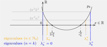
Figure 3: The parabola $p_{k}$ and the eigenvalues $\lambda_{n}^{\mp}$ for each $n\in{\mathbb{N}}_{0}$

Equivalently to (5.43) we obtain the quadratic equation for $\lambda_{n}$ given by

$$\lambda_{n}^{2}-\beta_{k}\lambda_{n}+\gamma_{k,n}=0$$

where

$$\beta_{k}:=\frac{4}{c_{k}^{4}}+\frac{1}{2c_{k}^{2}}=\frac{8+c_{k}^{2}}{2c_{k}^{4}},\qquad\gamma_{k,n}:=\frac{2}{c_{k}^{6}}-4\pi^{2}n^{2}=4\pi^{2}\left(k^{2}-n^{2}\right)$$

The solutions are

$$\lambda_{n}^{-}=\frac{\beta_{k}}{2}-\frac{1}{2}\sqrt{\beta_{k}^{2}-4\gamma_{k,n}},\qquad\lambda_{n}^{+}=\frac{\beta_{k}}{2}+\frac{1}{2}\sqrt{\beta_{k}^{2}-4\gamma_{k,n}}$$

Note that $\gamma_{k,k}=0$ and therefore

$$\lambda_{k}^{-}=0$$ (5.44)

is zero as well and $\lambda_{k}^{+}=\beta_{k}$. In case $n=0$ the quadratic equation (5.43) is already factorized, so we read off

$$\lambda_{0}^{-}=\frac{1}{2c_{k}^{2}},\qquad\lambda_{0}^{+}=\frac{4}{c_{k}^{4}},\qquad\lambda_{0}^{-}<\lambda_{0}^{+}$$

both of which are real numbers. So the argument of the square root is positive for $n=0$ and therefore for all $n$ (since $-\gamma_{k,n}$ is monotone increasing in $n$). Thus

Lemma 5.5 (Monotonicity).

The sequence $(\lambda_{n}^{-})_{n\in{\mathbb{N}}_{0}}$ is strictly monotone decreasing and $(\lambda_{n}^{+})_{n\in{\mathbb{N}}_{0}}$ is strictly monotone increasing.

Eigenvectors. Recall that we had fixed $k\in{\mathbb{N}}$, in other words the solution $(q_{k},p_{k})$ given by (5.40) of the Hamiltonian equation (5.30). We assume in addition $n\not=0$, that is $n\in{\mathbb{N}}$. Eigenvectors to the eigenvalues $\lambda_{n}^{\pm}$, notation $u_{n}^{\pm}$, can be found by setting $\eta_{n}:=1$, then according to equation  c) we define $\xi^{n}_{\pm}:=-\frac{1}{2\pi n}\left(\lambda_{n}^{\pm}-1/2c_{k}^{2}\right)$. The other Fourier coefficients we define to be equal $\mathrm{𝟎}$. With these choices an eigenvector for $\lambda_{n}^{\pm}$ is given by the function

$$u_{n}^{\pm}:\SS^{1}\to{\mathbb{R}}^{2},\quad\tau\mapsto\biggl{(}\underbrace{-\frac{1}{2\pi n}\left(\lambda_{n}^{\pm}-\frac{1}{2c_{k}^{2}}\right)}_{\xi^{n}_{\pm}}\sin 2\pi n\tau,\cos 2\pi n\tau\biggr{)}$$

Note that the coefficient $\xi^{n}_{+}$ is strictly negative and $\xi^{n}_{-}$ is strictly positive since

$$\lambda_{n}^{+}-\frac{1}{2c_{k}^{2}}>\lambda_{0}^{+}-\frac{1}{2c_{k}^{2}}>\lambda_{0}^{-}-\frac{1}{2c_{k}^{2}}=0$$

and similarly

$$\lambda_{n}^{-}-\frac{1}{2c_{k}^{2}}<\lambda_{0}^{-}-\frac{1}{2c_{k}^{2}}=0$$

Since $\xi^{n}_{+}>0$ we see that the eigenvector $u_{n}^{+}$ winds $n$ times counter-clockwise around the origin, while $u_{n}^{-}$ winds $n$ times clockwise around the origin since $\xi^{n}_{-}<0$. Therefore the winding numbers equal $\pm n$, in symbols

$$w(u_{n}^{\pm})=\pm n$$

Note that in the ode (local) case Lemma 5.5 would tell us that $w(\lambda_{n}^{+})=n$, but in the non-local case we cannot yet conclude independence of the choice of an eigenvector.

Remark 5.6 (Case $n=0$).

Eigenvalue $\lambda_{0}^{-}=1/2c_{k}^{2}$. In c) we choose $\eta_{0}:=1$ and set all other Fourier coefficients zero. Then $u_{0}^{-}=(0,1)$ is an eigenvector to the eigenvalue $\lambda_{0}^{-}$. Since the function $u_{0}^{-}$ is constant, its winding number vanishes, in symbols $w(u_{0}^{-})=0$.
Eigenvalue $\lambda_{0}^{+}=4/c_{k}^{4}$. By e) we can choose $\xi_{0}:=1$ and all other Fourier coefficients equal zero. For these choices $u_{0}^{+}=(1,0)$ is an eigenvector to the eigenvalue $\lambda_{0}^{+}$. By constancy the winding number is $\mathrm{𝟎}$, in symbols $w(u_{0}^{+})=0$.

Remark 5.7 (Geometric multiplicity of eigenvalues $\lambda_{n}^{\pm}$ is $\geq 2$ for $n\not=0,k$).

Instead of using c) and d) one can use a) and e). Setting $\eta^{n}:=1$ equation a) motivates to define $\xi_{n}^{\pm}:=-\frac{1}{2\pi n}\left(\lambda_{n}^{+}-1/2c_{k}^{2}\right)$. With these choices a further eigenvector for $\lambda_{n}^{\pm}$ is given by the function

$$v_{n}^{\pm}:\SS^{1}\to{\mathbb{R}}^{2},\quad\tau\mapsto\biggl{(}\underbrace{\frac{1}{2\pi n}\left(\lambda_{n}^{\pm}-\frac{1}{2c_{k}^{2}}\right)}_{\xi_{n}^{\pm}}\cos 2\pi n\tau,\sin 2\pi n\tau\biggr{)}$$

We observe that, just as above, the winding number of the eigenvector $v_{n}^{+}$ is $n$, and of $v_{n}^{-}$ it is $-n$, in symbols

$$w(v_{n}^{\pm})=\pm n$$

Case $n=k$ and the eigenvalues $\widehat{\lambda}_{k}^{\pm}$

In the case $n=k$ we obtain from equations b) and f) the quadratic equation

$$\underbrace{\left(\widehat{\lambda}_{k}-\frac{1}{2c_{k}^{2}}\right)\left(\widehat{\lambda}_{k}+\frac{12}{c_{k}^{4}}\right)}_{\text{polynomial $\widehat{p}_{k}(x)$ in variable $x=\widehat{\lambda}_{k}$}}=36\pi^{2}k^{2}$$ (5.45)

The polynomial $\widehat{p}_{k}(x)$ is illustrated by Figure 4.

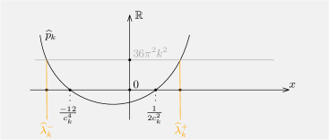
Figure 4: Parabola $\widehat{p}_{k}$ in the variable $x=\widehat{\lambda}_{k}$ given by (5.45)

Eigenvalues. Equivalently we obtain the quadratic equation for $\widehat{\lambda}_{k}$ given by

$$\widehat{\lambda}_{k}^{2}-B_{k}\widehat{\lambda}_{k}+C_{k}=0$$

where

$$\begin{split}B_{k}&:=\frac{1}{2c_{k}^{2}}-\frac{12}{c_{k}^{4}}=\beta_{k}-\frac{16}{c_{k}^{4}},\qquad\quad\beta_{k}:=\frac{4}{c_{k}^{4}}+\frac{1}{2c_{k}^{2}}=\frac{8+c_{k}^{2}}{2c_{k}^{4}}\\ C_{k}&:=-\frac{6}{c_{k}^{6}}-36\pi^{2}k^{2}=-48\pi^{2}k^{2}\end{split}$$

with $c_{k}<1$ given by (5.39). The solutions are

$$\widehat{\lambda}_{k}^{-}=\frac{B_{k}}{2}-\frac{1}{2}\sqrt{B_{k}^{2}-4C_{k}},\qquad\widehat{\lambda}_{k}^{+}=\frac{B_{k}}{2}+\frac{1}{2}\sqrt{B_{k}^{2}-4C_{k}}$$

Eigenvectors. Eigenvectors to the eigenvalues $\widehat{\lambda}_{k}^{\pm}$, notation $u_{k}^{\pm}$, can be found by setting $\eta^{k}:=1$, then equation b) motivates to define

$$\xi_{k}:=\frac{1}{6\pi k}\left(\widehat{\lambda}_{k}^{\pm}-1/2c_{k}^{2}\right)$$

The other Fourier coefficients we define to be equal $\mathrm{𝟎}$. With these choices an eigenvector for $\widehat{\lambda}_{k}^{\pm}$ is given by the function

$$v_{k}^{\pm}:\SS^{1}\to{\mathbb{R}}^{2},\quad\tau\mapsto\left(\frac{1}{6\pi k}\left(\widehat{\lambda}_{k}^{\pm}-\frac{1}{2c_{k}^{2}}\right)\cos 2\pi k\tau,\sin 2\pi k\tau\right)$$

As one sees from Figure 4 the following inequalities hold

$$\widehat{\lambda}_{k}^{-}<-\frac{12}{c_{k}^{4}}<0<\frac{1}{2c_{k}^{2}}<\widehat{\lambda}_{k}^{+}$$

Therefore $\widehat{\lambda}_{k}^{+}-\frac{1}{2c_{k}^{2}}>0$ and $\widehat{\lambda}_{k}^{-}-\frac{1}{2c_{k}^{2}}<0$ and hence the winding number are

$$w(v_{k}^{\pm})=\pm k$$

5.7 Disjoint families and winding numbers

Consider the two quadratic polynomials $p_{k}$ and $\widehat{p}_{k}$ in the variable $x=\lambda_{n}$ given by the left hand sides of (5.43) and (5.45), namely

$$p_{k}(x):=\left(x-\frac{1}{2c_{k}^{2}}\right)\left(x-\frac{4}{c_{k}^{4}}\right)$$

and

$$\widehat{p}_{k}(x):=\left(x-\frac{1}{2c_{k}^{2}}\right)\left(x+\frac{12}{c_{k}^{4}}\right)$$

These two polynomials have a common zero at $x=1/2c_{k}^{2}$, they are sketched in Figure 5.

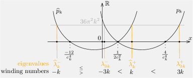
Figure 5: The parabolas $\widehat{p}_{k}$ and $p_{k}$, eigenvalues and winding numbers

For $n=3k$ there is equality $4\pi^{2}n^{2}=36\pi^{2}k^{2}$ and the intersection of $\widehat{p}_{k}$ and $p_{k}$ with the horizontal line $\{36\pi^{2}k^{2}\}$ consists of 4 points whose $x$-coordinates are the following eigenvalues in the following order

$$\widehat{\lambda}_{k}^{-}<\lambda_{3k}^{-}<\widehat{\lambda}_{k}^{+}<\lambda_{3k}^{+}$$

Proposition 5.8.

For any $n\in{\mathbb{N}}_{0}$ the $\lambda_{n}^{\mp}$ are different from $\widehat{\lambda}_{k}^{-}$ and from $\widehat{\lambda}_{k}^{+}$, in symbols

$$\lambda_{n}^{\mp}\not=\widehat{\lambda}_{k}^{-},\qquad\lambda_{n}^{\mp}\not=\widehat{\lambda}_{k}^{+},\qquad n\in{\mathbb{N}}_{0}$$

Proof.

Note that $\widehat{\lambda}_{k}^{-}<0$ is negative. On the other hand $\lambda_{n}^{+}>0$, for $n\in{\mathbb{N}}_{0}$, as well as $\lambda_{0}^{-}>0$ are all positive. Therefore it suffices to show that $\widehat{\lambda}_{k}^{-}\not=\lambda_{n}^{-}$ for every $n\in{\mathbb{N}}$.

Suppose by contradiction that there are $i,j\in\{+,-\}$ such that $\widehat{\lambda}_{k}^{i}=\lambda_{n}^{j}=:\lambda$ for some $n\in{\mathbb{N}}_{0}$. The idea is to construct two polynomials $P(z)$ and $Q(z)$ which have a common zero at $z=c_{k}^{2}$ and then use algebra to show that there cannot be two such polynomials.
Step 0. It is useful to consider the field extension ${\mathbb{Q}}(\pi)$ of ${\mathbb{Q}}$ which is a subfield of ${\mathbb{R}}$, that is ${\mathbb{Q}}\subset{\mathbb{Q}}(\pi)\subset{\mathbb{R}}$. Elements of ${\mathbb{Q}}(\pi)$ have the following form. Given rational polynomials $p,q\in{\mathbb{Q}}[x]$ with $q\not\equiv 0$ not the zero polynomial, numbers in ${\mathbb{Q}}(\pi)$ are given by $p(\pi)/q(\pi)$. Note that by the theorem of Lindemann [Lin82], see [Hil93] for an elegant proof by Hilbert, the number $\pi$ is transcendental and therefore $q(\pi)\not=0$ is non-zero.
Step 1. The definition of the polynomial

$$Q(z):=z^{3}+a_{0},\qquad a_{0}:=-(c_{k}^{2})^{3}\stackrel{{\scriptstyle(\ref{eq:c_k})}}{{=}}-\frac{1}{2\pi^{2}k^{2}}\in{\mathbb{Q}}(\pi)$$ (5.46)

is motivated by the goal that it has a zero at the point $z=c_{k}^{2}$ given by (5.39). Here ${\mathbb{Q}}(\pi)$ is the field extension of ${\mathbb{Q}}$ by adjoining $\pi$ from Step 0. The field extension ${\mathbb{Q}}(\pi)$ is isomorphic to the field ${\mathbb{Q}}(x)$ of rational functions.
Step 2. Divide the polynomial identity $\widehat{p}_{k}(\lambda)=36\pi^{2}k^{2}$ by $p_{k}(\lambda)=4\pi^{2}n^{2}$ to get that

$$\frac{\lambda+\frac{12}{c_{k}^{4}}}{\lambda-\frac{4}{c_{k}^{4}}}=\frac{36\pi^{2}k^{2}}{4\pi^{2}n^{2}}=9\frac{k^{2}}{n^{2}}$$

Now multiply by the denominator to get that

$$\lambda+\frac{12}{c_{k}^{4}}=9\frac{k^{2}}{n^{2}}\left(\lambda-\frac{4}{c_{k}^{4}}\right)$$

Resolving for $\lambda$ yields

$$\lambda=\frac{4}{c_{k}^{4}}\cdot\frac{9\frac{k^{2}}{n^{2}}+3}{9\frac{k^{2}}{n^{2}}-1}=\frac{4}{c_{k}^{4}}\cdot\frac{9k^{2}+3n^{2}}{9k^{2}-n^{2}}$$

Consequently

$$\lambda\in\frac{1}{c_{k}^{4}}{\mathbb{Q}}$$ (5.47)

Now evaluate $\widehat{p}_{k}$ at $\lambda$ to get (since $\lambda:=\widehat{\lambda}_{k}^{i}$) that

$$\begin{split}0&=\widehat{p}_{k}(\lambda)-36\pi^{2}k^{2}\\ &=\left(\lambda-\frac{1}{2c_{k}^{2}}\right)\left(\lambda+\frac{12}{c_{k}^{4}}\right)-36\pi^{2}k^{2}\\ \end{split}$$ (5.48)

Multiplication by ${c_{k}}^{8}$ and division by $-36\pi^{2}k^{2}$ leads to

$$\begin{split}0&=\frac{\lambda^{2}c_{k}^{8}+\lambda c_{k}^{4}\left(12-c_{k}^{2}/2\right)-6c_{k}^{2}}{-36\pi^{2}k^{2}}+c_{k}^{8}\\ &=-\frac{4}{9\pi^{2}k^{2}}\left(\frac{9k^{2}+3n^{2}}{9k^{2}-n^{2}}\right)^{2}+\frac{1}{18\pi^{2}k^{2}}\left(\frac{9k^{2}+3n^{2}}{9k^{2}-n^{2}}\right)c_{k}^{2}\\ &\quad-\frac{4}{3\pi^{2}k^{2}}\left(\frac{9k^{2}+3n^{2}}{9k^{2}-n^{2}}\right)+\frac{1}{18\pi^{2}k^{2}}\left(\frac{9k^{2}+3n^{2}}{9k^{2}-n^{2}}\right)c_{k}^{2}+c_{k}^{8}\\ &=P(c_{k}^{2})\end{split}$$ (5.49)

where the polynomial $P$ is given by

$$P(z)=z^{4}+b_{1}z+b_{0},\qquad b_{0},b_{1}\in{\mathbb{Q}}(\pi)$$

and the coefficients $b_{0}$ and $b_{1}$ – according to (5.49) – by

$$\begin{split}b_{0}&=-\frac{4}{3\pi^{2}k^{2}}\frac{9k^{2}+3n^{2}}{9k^{2}-n^{2}}\left(\frac{3k^{2}+n^{2}}{9k^{2}-n^{2}}+1\right)=-\frac{48}{\pi^{2}}\frac{3k^{2}+n^{2}}{(9k^{2}-n^{2})^{2}}<0\\ b_{1}&=\frac{1}{9\pi^{2}k^{2}}\left(\frac{9k^{2}+3n^{2}}{9k^{2}-n^{2}}\right)\end{split}$$

We define a linear polynomial in $z$ with coefficients in the field ${\mathbb{Q}}(\pi)$ by the formula

$$R(z):=P(z)-zQ(z)=(b_{1}-a_{0})z+b_{0}$$

Since $z=c_{k}^{2}$ is a zero of $P$ by (5.49) and of $Q$ by (5.46), it is a zero of the linear polynomial $R$.
Since $b_{0}\not=0$ it follows that $b_{1}-a_{0}\not=0$: otherwise $R\equiv b_{0}\not=0$ would not have a zero at all. Since $0=R(c_{k}^{2})=(b_{1}-a_{0})c_{k}^{2}+b_{0}$ we get that $c_{k}^{2}=-b_{0}/(b_{1}-a_{0})\in{\mathbb{Q}}(\pi)$, that is $c_{k}^{2}$ is of the form $p(\pi)/q(\pi)$ where $p,q\in{\mathbb{Q}}[z]$.

We derive a contradiction: Evaluate (5.46) at $z=\frac{p(\pi)}{q(\pi)}=c_{k}^{2}\in(0,1)$ to get

$$0=Q(c_{k}^{2})=\frac{p(\pi)^{3}}{q(\pi)^{3}}-\frac{1}{2\pi^{2}k^{2}}$$

Multiply the identity by $q(\pi)^{3}\left(2\pi^{2}k^{2}\right)$ to get that

$$0=\underbrace{p(\pi)^{3}\left(2\pi^{2}k^{2}\right)}_{\deg=2\mod 3}-\underbrace{q(\pi)^{3}}_{\deg=0\mod 3}$$

Consider the polynomial $s:=p^{3}r-q^{3}\in{\mathbb{Q}}[z],$ where $r(z):=2k^{2}z^{2}$.
Claim. $s\not\equiv 0$
Proof of claim. This follows from considering the degrees. Note that

$$\deg r=2\mod 3,\qquad\deg p^{3}=0\mod 3,\qquad\deg q^{3}=0\mod 3$$

Therefore

$$\deg p^{3}r=\deg p^{3}+\deg r=2\mod 3,\qquad\deg q^{3}=0\mod 3$$

Hence $p^{3}r\not=q^{3}$ and consequently $s\not\equiv 0$. This proves the claim.

In view of the claim we found a non-zero polynomial $s$ with rational coefficients and the property that $s(\pi)=0$. But this contradicts the theorem of Lindemann as explained earlier. ∎

Corollary 5.9 (Well-defined winding number).

For every $n\in{\mathbb{N}}_{0}$ we define the winding numbers

$$w(\lambda_{n}^{-}):=-n,\quad w(\lambda_{n}^{+}):=n,\quad w(\widehat{\lambda}_{k}^{-}):=-k,\quad w(\widehat{\lambda}_{k}^{+}):=k$$

In view of Proposition 5.8 these winding numbers are well-defined and, in view of the discussion before, correspond to the winding number of an arbitrary eigenvector of the eigenvalue.

$\mathrm{spec}\,L_{\mathcal{S}}$	$\lambda_{n}^{-}$	$\lambda_{k}^{-}=0$	$\lambda_{0}^{-}$	$\lambda_{0}^{+}$	$\lambda_{k}^{+}$	$\lambda_{n}^{+}$
		$\widehat{\lambda}_{k}^{-}$			$\widehat{\lambda}_{k}^{+}$
$m$	$2$	$1$	$1$	$1$	$1$	$2$
$w$	$-n$	$-k$	$\mathrm{𝟎}$	$\mathrm{𝟎}$	$k$	$n$

Figure 6: Multiplicities $m$ and winding numbers $w$ of eigenvalues, $n\in{\mathbb{N}}\setminus\{k\}$

Proposition 5.10.

At a critical point $(x_{k},y_{k})$ of ${\mathcal{A}}_{\mathcal{H}}$, see (5.40), it holds that

$$\alpha({\mathcal{S}}_{(x_{k},y_{k})})=w(\widehat{\lambda}_{k}^{-})=-k,\qquad p({\mathcal{S}}_{(x_{k},y_{k})})=1$$

and with the definitions ${\mu_{\rm CZ}}:=2\alpha+p$ and ${\mu^{\rm CZ}}:=-{\mu_{\rm CZ}}$ we obtain

$${\mu_{\rm CZ}}(x_{k},y_{k})=-2k+1,\qquad{\mu^{\rm CZ}}(x_{k},y_{k})=2k-1$$

Proof.

With ${\mathcal{S}}:={\mathcal{S}}_{(x_{k},y_{k})}$ we recall the definition of $\alpha$, namely

$$\alpha({\mathcal{S}}):=\max\{w(\lambda)\mid\lambda\in(-\infty,0)\mathop{\cap}\mathrm{spec}\,L_{\mathcal{S}}\}\in{\mathbb{Z}}$$

Observe that $\widehat{\lambda}_{k}^{-}<0$, see Figure 4, and $w(\widehat{\lambda}_{k}^{-})=-k$, see Figure 6. Therefore $\alpha({\mathcal{S}})\geq-k$. To show the reverse inequality $\alpha({\mathcal{S}})\leq-k$ we need to check non-negativity of all eigenvalues with winding number $>-k$. By Figure 6 the eigenvalues of winding number $>-k$ are of three types:

• $\lambda_{n}^{-}$ for $n<k$: In this case $\lambda_{n}^{-}>\lambda_{k}^{-}=0$ for every $n<k$ by monotonicity, see Lemma 5.5, and (5.44).

• $\lambda_{n}^{+}$ for all $n\in{\mathbb{N}}_{0}$: In this case $\lambda_{n}^{+}>0$ for every $n\in{\mathbb{N}}_{0}$ by Figure 3

• $\widehat{\lambda}_{k}^{+}$: In this case $\widehat{\lambda}_{k}^{+}>0$ by Figure 4.

This proves that $\alpha({\mathcal{S}})=-k$.

Because there exists a non-negative eigenvalue, namely $\lambda_{k}^{-}=0$, with the same winding number $-k$ as the negative eigenvalue $\widehat{\lambda}_{k}^{-}<0$ that realizes the maximal winding number $\alpha({\mathcal{S}}_{(x_{k},y_{k})})$ among negative eigenvalues, we get that

$$p({\mathcal{S}}_{(x_{k},y_{k})})=1$$

∎

References

- [AFS19a] Peter Albers, Urs Frauenfelder, and Felix Schlenk. A compactness result for non-local unregularized gradient flow lines. J. Fixed Point Theory Appl., 21(1):34–61, 2019. arXiv:1802.07445.
- [AFS19b] Peter Albers, Urs Frauenfelder, and Felix Schlenk. An iterated graph construction and periodic orbits of Hamiltonian delay equations. J. Differential Equations, 266(5):2466–2492, 2019. arXiv:1802.07449.
- [AFS20] Peter Albers, Urs Frauenfelder, and Felix Schlenk. Hamiltonian delay equations—examples and a lower bound for the number of periodic solutions. Adv. Math., 373:107319, 17, 2020. arXiv:1802.07453.
- [Arn67] V. I. Arnol′d. On a characteristic class entering into conditions of quantization. Funkcional. Anal. i Priložen., 1:1–14, 1967.
- [AS06] Alberto Abbondandolo and Matthias Schwarz. On the Floer homology of cotangent bundles. Comm. Pure Appl. Math., 59(2):254–316, 2006.
- [AS15] Alberto Abbondandolo and Matthias Schwarz. The role of the Legendre transform in the study of the Floer complex of cotangent bundles. Comm. Pure Appl. Math., 68(11):1885–1945, 2015.
- [BOV21] Vivina Barutello, Rafael Ortega, and Gianmaria Verzini. Regularized variational principles for the perturbed Kepler problem. Adv. Math., 383:Paper No. 107694, 64, 2021. arXiv:2003.09383.
- [FW21] Urs Frauenfelder and Joa Weber. The shift map on Floer trajectory spaces. J. Symplectic Geom., 19(2):351–397, 2021. arXiv:1803.03826.
- [Hil93] David Hilbert. Über die Transcendenz der Zahlen und . Mathematische Annalen, 43(2):216–219, 1893.
- [HWZ95] H. Hofer, K. Wysocki, and E. Zehnder. Properties of pseudo-holomorphic curves in symplectisations. II. Embedding controls and algebraic invariants. Geom. Funct. Anal., 5(2):270–328, 1995.
- [LC20] Tullio Levi-Civita. Sur la régularisation du problème des trois corps. Acta Math., 42:99–144, 1920.
- [Lin82] F. Lindemann. Ueber die Zahl . Math. Ann., 20(2):213–225, 1882.
- [Mas65] V. P. Maslov. Theory of Perturbations and Asymptotic Methods. izd. MGU, 1965.
- [Mos70] Jürgen Moser. Regularization of Kepler’s problem and the averaging method on a manifold. Comm. Pure Appl. Math., 23:609–636, 1970.
- [SW06] Dietmar Salamon and Joa Weber. Floer homology and the heat flow. Geom. Funct. Anal., 16(5):1050–1138, 2006.
- [Vit98] Claude Viterbo. Functors and computations in Floer homology with applications, II. Preprint Université Paris-Sud no. 98-15, 1998.
- [Web02] Joa Weber. Perturbed closed geodesics are periodic orbits: Index and transversality. Math. Z., 241(1):45–82, 2002.
- [Web17] Joa Weber. Topological methods in the quest for periodic orbits. Publicações Matemáticas do IMPA. [IMPA Mathematical Publications]. Instituto Nacional de Matemática Pura e Aplicada (IMPA), Rio de Janeiro, 2017. 31o Colóquio Brasileiro de Matemática. vii+248 pp. ISBN: 978-85-244-0439-9. Access book. Version on arXiv:1802.06435. An extended version to appear in the EMS Lecture Series of Mathematics.