Anomalous gravitomagnetic moment and non-universality of the axial vortical effect
at finite temperature

Abstract

The coupling between the spin of a massive Dirac fermion and the angular momentum of the medium, i.e. the gravitomagnetic moment, is shown here to be renormalized by QED interactions at finite temperature. This means that the anomalous gravitomagnetic moment (AGM) does not vanish, and implies that thermal effects can break the Einstein equivalence principle in quantum field theory, as argued previously. We also show that the AGM causes radiative corrections to the axial current of massive fermions induced by vorticity in quantum relativistic fluids, similarly to the previous findings for massless fermions. The radiative QCD effects on the AGM should significantly affect the production of polarized hadrons in heavy-ion collisions.

I Introduction

Recent experiments Adamczyk et al. (2017); Adam et al. (2018, 2019) at the Relativistic Heavy Ion Collider (RHIC) have opened the possibility to study the effects of vorticity and magnetic field on the production of polarized hadrons in relativistic heavy-ion collisions, see Becattini and Lisa (2020) for a recent review. The coupling between the spin and vorticity of the quark gluon plasma Liang and Wang (2005); Kharzeev (2006); Becattini et al. (2008) induces a polarization of the hadrons emitted from the fluid, which can be measured in experiments. The spin and the polarization of a spin $1/2$ particle, like the $\Lambda$ hyperon, is deeply connected to the axial current of the particle. In a rotating medium, the coupling between the spin of a fermion and rotation of the medium Vilenkin (1979) also induces a thermal effect on the axial current, known as the Axial Vortical Effect (AVE).

The AVE is a macroscopic quantum effect describing the axial charge separation along the rotation of the fluid Landsteiner et al. (2011a); Gao et al. (2012); Kharzeev et al. (2016). In the case of a system composed of massless fermions, one can give a simple intuitive picture of the phenomenon. Indeed, as a result of the coupling between the fermions’ spin and the rotation of the medium, the spins of the fermions are preferably aligned along the angular momentum vector of the medium. Then, since for massless fermions chirality coincides with helicity (note that for antifermions, chirality and helicity are opposite), most of the right-handed particles will move along the direction of the vorticity (pseudo)vector, while most of the left-handed particles will move in the opposite direction. This flow causes the net separation between the right- and left-handed particles that we refer to as the AVE. Since the AVE is driven by spin-rotation coupling, it can be realized even in a global thermal equilibrium, where the expectation value of the axial current is given by  Buzzegoli and Becattini (2018)

$$\langle\widehat{j}^{\mu}_{\textup{A}}\rangle=n_{\textup{A}}u^{\mu}+W^{\textup{A}}\frac{\omega^{\mu}}{T}.$$

where $n_{A}$ is the density of axial charge, $u$ is the fluid velocity, $\omega$ is the vorticity of the medium, and $T$ is the temperature. For free massless fermions the AVE conductivity $W^{\textup{A}}$ is found to be Vilenkin (1979); Landsteiner et al. (2011a); Gao et al. (2012)

$$W^{\textup{A}}=\frac{T^{3}}{6}+\frac{\mu^{2}+\mu_{\textup{A}}^{2}}{2\pi^{2}}T,$$

where $\mu$ is the vector chemical potential and $\mu_{\textup{A}}$ is the axial chemical potential.

The AVE shares many similarities with other non-dissipative macroscopic quantum effects, such as the Chiral Magnetic Effect (CME) Kharzeev (2006); Kharzeev et al. (2008); Fukushima et al. (2008) and the Chiral Vortical Effect (CVE) Kharzeev and Zhitnitsky (2007); Erdmenger et al. (2009). However, even though both CME and CVE originate from the chiral anomaly Kharzeev (2014), the link between AVE and anomalies is still under discussion, see  Landsteiner et al. (2011b); Jensen et al. (2013); Kalaydzhyan (2014); Golkar and Sethi (2016); Avkhadiev and Sadofyev (2017); Glorioso et al. (2019); Flachi and Fukushima (2018); Buzzegoli et al. (2017); Buzzegoli and Becattini (2018); Stone and Kim (2018); Prokhorov et al. (2020). First, both the axial current and the vorticity are axial vectors, and therefore AVE does not require parity breaking. Second, the AVE conductivity is not protected against radiative corrections: explicit calculations in massless quantum electrodynamics (QED) and quantum chromodynamics (QCD) show that AVE conductivity is renormalized by interactions Hou et al. (2012); Golkar and Son (2015).

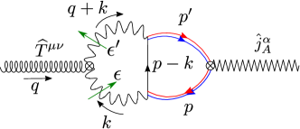
Figure 1: The Feynman diagram describing the radiative corrections to AVE conductivity. Red and blue lines represent right and left chiralities of the fermions, and the green arrows represent the photon polarization.

This correction only affects the finite-temperature part of the AVE conductivity, while the parts proportional to the axial chemical potential and the vector chemical potential are unaltered by interactions. Indeed, at second order in QED coupling constant $e$, the AVE conductivity for a massless fermion is given by Hou et al. (2012); Golkar and Son (2015)

$$W^{\textup{A}}=\left(\frac{1}{6}+\frac{e^{2}}{24\pi^{2}}\right)T^{3}.$$

This correction is given solely by the diagram in Fig. 1. Higher order corrections are non-vanishing only if they are given by diagrams in which the axial current is inserted through the anomalous triangle subdiagram Golkar and Son (2015).

The radiative corrections to AVE in QED can be interpreted as driven by the interaction of a graviton with the photon cloud surrounding the fermion. Indeed, we may understand the coupling between the chirality of fermions and rotation of the medium induced by this diagram as follows. Suppose the lower fermion line inside the loop in Fig. 1 has a right chirality. Then it couples more effectively to photons having a polarization parallel to the fermion spin. Following the loop in the figure, those photons then interact with the rotation of the medium (represented by the insertion of stress-energy tensor in the diagram) forcing their polarization to rotate – so when they couple to the fermion in the loop again, they can induce the chirality flip of the fermion, and transform it into a left-handed one. Note that this requires the presence of photons in the rotating fluid, which in thermal equlibrium implies a finite temperature. At zero temperature, the photon cloud is part of the coherent state of a charged fermion, and thus rotates together with it. At finite temperature, the thermal bath possesses its own photons, and mixing between these photons and the photons that form the coherent cloud of the fermion can cause the rotation of the fermion’s polarization.

In analogy with the magnetic moment, the quantity that describes the coupling of a fermion’s spin to rotation is a gravitomagnetic moment. The picture discussed above thus suggests that we can describe the radiative correction to this quantity as an Anomalous Gravitomagnetic Moment (AGM), as Fig. 1 is analogous to the diagram describing the anomalous magnetic moment in QED. In this work we validate the connection between the AGM and the radiative corrections to the AVE for the case of a massive fermion. We show that the gravitomagnetic moment of a massive fermion in thermal equilibrium is indeed anomalous, and that the radiative corrections to the AVE in the low temperature regime are due to the gravitomagnetic moment.

The emergence of the AGM may seem surprising, as the Einstein equivalence principle forbids the appearance of an anomalous spin-rotation coupling Kobzarev and Okun (1962); Teryaev (2016). In the language of quantum field theory, the equivalence principle is translated into the Lorentz invariance of the local coupling of gravitational fields to the stress-energy tensor Cho and Hari Dass (1976). This is why the presence of an AGM is excluded for both elementary Cho and Hari Dass (1976) and composite Teryaev (2016, 2007) particles. However, an explicit renormalization of stress-energy tensor for massive QED at finite temperature has demonstrated that the effects of temperature break the weak equivalence principle (i.e., gravitational and inertial mass are no longer equivalent) Donoghue et al. (1984, 1985). The equivalence principle violation can be ascribed to the fact that a finite temperature breaks the Lorentz invariance of the vacuum and that, in the presence of a thermal bath, one can genuinely discern if the system is under acceleration or under the effect of a gravitational field by making measurements in reference to the thermal bath. Thus, we can expect, and indeed have found, the emergence of the AGM at finite temperature.

This paper is organized as follows. In Sec. II we evaluate the AVE conductivity in the low temperature regime for a non-relativistic particle and show that the radiative corrections to this conductivity can be quantitatively derived from the anomalous gravitomagnetic moment. In Sec. III we introduce the gravitomagnetic moment of a Dirac fermion and evaluate the radiative correction to it at one-loop level in finite temperature QED. In Sec. IV we use the scattering theory in linearized gravity to obtain a formula which connects the gravitomagnetic moment to the matrix elements of the stress-energy tensor. A summary and a discussion of the results are given in Sec. V. The details on the renormalization of the stress-energy tensor at finite temperature and the evaluation of the related Feynamn diagrams are given respectively in appendix C and D. In App. A we review how finite temperature effects lead to a difference between inertial and gravitational mass.

II Radiative corrections to the axial vortical effect for a massive field

In this section we evaluate the radiative corrections to the axial vortical effect (AVE) conductivity $W^{\textup{A}}$ for a massive Dirac field in a low temperature regime. We obtain the AVE conductivity starting from the corresponding Kubo formula that involves the thermal correlator between the stress-energy tensor and the axial current operators. As any quantum operator can be written in terms of its matrix elements by expanding it in multi-particle states Weinberg (2005), it then follows that the AVE conductivity can be obtained by considering the radiative corrections to the following matrix elements:

$$\langle p^{\prime},s^{\prime}|\widehat{T}^{\mu\nu}(0)|p,s\rangle,\quad\langle p^{\prime},s^{\prime}|\widehat{j}_{\textup{A}}^{\mu}(0)|p,s\rangle,$$

where $\widehat{T}^{\mu\nu}$ is the stress-energy tensor, $\widehat{j}_{\textup{A}}$ is the axial current, and $|p,s\rangle$ is the state representing a single fermion with momentum $p$ and spin $s$. The main strategy we adopt to evaluate the radiative corrections of $W^{\textup{A}}$ is to include the effects of the interactions by renormalazing the matrix elements above using finite temperature QED. After renormalization, the formula for the AVE conductivity is formally identical to the one in the free field case, the only difference being the values of the renormalized matrix elements. In particular, the thermal correlator will act solely on the fermionic creation and annihilation operators and can be readily written down. An equivalent approach to evaluating statistical averages is described in the textbook Groot et al. (1980), where the density matrix is written in terms of its “in-picture” matrix elements. In this section we derive the conductivity $W^{\textup{A}}$, while the renormalization of the matrix elements is performed in App. C.

The AVE conductivity $W^{\textup{A}}$ for a massive Dirac field is given by the thermal correlator between the axial current and the total angular momentum of the system and can be written as Buzzegoli et al. (2017)

$$\begin{split}W^{\textup{A}}=2\int_{0}^{\beta}\frac{{\rm d}\tau}{\beta}\int{\rm d}^{3}x\,x^{1}\langle\widehat{T}^{02}(-\mathrm{i}\tau,\mathchoice{\mbox{\boldmath$\displaystyle\mathbf{x}$}}{\mbox{\boldmath$\textstyle\mathbf{x}$}}{\mbox{\boldmath$\scriptstyle\mathbf{x}$}}{\mbox{\boldmath$\scriptscriptstyle\mathbf{x}$}})\,\widehat{j}^{3}_{\textup{A}}(0)\rangle_{\textup{T,c}},\end{split}$$ (1)

where the symbol $\langle\cdots\rangle_{T}$ denotes thermal averages performed in the rest frame of thermal bath $u=(1,\mathchoice{\mbox{\boldmath$\displaystyle\mathbf{0}$}}{\mbox{\boldmath$\textstyle\mathbf{0}$}}{\mbox{\boldmath$\scriptstyle\mathbf{0}$}}{\mbox{\boldmath$\scriptscriptstyle\mathbf{0}$}})$ with the familiar homogeneous global equilibrium density operator in the grand-canonical ensemble

$$\widehat{\rho}=\frac{1}{Z}\exp[-\beta(x)\cdot\widehat{P}]$$

where $\widehat{P}^{\mu}$ is the total four-momentum of the system. The subscript $c$ on the thermal average in (1) denotes the connected part of the correlator, that is, for the simplest case of two operators:

$$\langle\widehat{O}_{1}\widehat{O}_{2}\rangle_{c}\equiv\langle\widehat{O}_{1}\widehat{O}_{2}\rangle-\langle\widehat{O}_{1}\rangle\langle\widehat{O}_{2}\rangle.$$

As mentioned in the beginning of this section, the stress-energy tensor can be decomposed in the multi-particle Hilbert space basis and can be written as a combination of creation and annihilation operators. We thus denote with ${\widehat{a}}^{\dagger}_{\tau}$ and ${\widehat{b}}^{\dagger}_{\tau}$ the creation operators of, respectively, the particle and anti-particle state of Dirac field with momentum $p$ and spin $\tau$, covariantly normalized as:

$$\{{\widehat{a}}_{\sigma}(q),{\widehat{a}}^{\dagger}_{\tau^{\prime}}(q^{\prime})\}=2\,\varepsilon_{q}\,\delta_{\tau\tau^{\prime}}\delta^{3}(\mathchoice{\mbox{\boldmath$\displaystyle\mathbf{q}$}}{\mbox{\boldmath$\textstyle\mathbf{q}$}}{\mbox{\boldmath$\scriptstyle\mathbf{q}$}}{\mbox{\boldmath$\scriptscriptstyle\mathbf{q}$}}-\mathchoice{\mbox{\boldmath$\displaystyle\mathbf{q}$}}{\mbox{\boldmath$\textstyle\mathbf{q}$}}{\mbox{\boldmath$\scriptstyle\mathbf{q}$}}{\mbox{\boldmath$\scriptscriptstyle\mathbf{q}$}}^{\prime}),\qquad\{{\widehat{b}}_{\sigma}(q),{\widehat{b}}^{\dagger}_{\tau^{\prime}}(q^{\prime})\}=2\,\varepsilon_{q}\,\delta_{\tau\tau^{\prime}}\delta^{3}(\mathchoice{\mbox{\boldmath$\displaystyle\mathbf{q}$}}{\mbox{\boldmath$\textstyle\mathbf{q}$}}{\mbox{\boldmath$\scriptstyle\mathbf{q}$}}{\mbox{\boldmath$\scriptscriptstyle\mathbf{q}$}}-\mathchoice{\mbox{\boldmath$\displaystyle\mathbf{q}$}}{\mbox{\boldmath$\textstyle\mathbf{q}$}}{\mbox{\boldmath$\scriptstyle\mathbf{q}$}}{\mbox{\boldmath$\scriptscriptstyle\mathbf{q}$}}^{\prime}),$$

where $\varepsilon_{q}=\sqrt{\mathchoice{\mbox{\boldmath$\displaystyle\mathbf{q}$}}{\mbox{\boldmath$\textstyle\mathbf{q}$}}{\mbox{\boldmath$\scriptstyle\mathbf{q}$}}{\mbox{\boldmath$\scriptscriptstyle\mathbf{q}$}}^{2}+m^{2}}$. The spinors for particle $u_{\tau}(q)$ and for anti-particle $v_{\tau}(q)$ are normalized as

$$u^{\dagger}_{\tau}(q)u_{\tau^{\prime}}(q)=\delta_{\tau\tau^{\prime}},\qquad v^{\dagger}_{\tau}(q)v_{\tau^{\prime}}(q)=\delta_{\tau\tau^{\prime}}.$$

Furthermore, taking advantage of the fact that $\widehat{T}^{\mu\nu}$ is an additive operator, it is uniquely determined by Weinberg (2005):

$$\begin{split}\widehat{T}^{\mu\nu}(x)=&\frac{1}{(2\pi)^{3}}\sum_{\tau,\tau^{\prime}}\int{\rm d}^{3}q^{\prime}\int{\rm d}^{3}q\,{\widehat{a}}^{\dagger}_{\tau^{\prime}}(q^{\prime}){\widehat{a}}_{\tau}(q){\rm e}^{\mathrm{i}(q-q^{\prime})\cdot x}\bar{u}_{\tau^{\prime}}(q^{\prime})_{A}M^{\mu\nu}_{++}(q,q^{\prime})_{AB}\,u_{\tau}(q)_{B}+\\ &+\frac{1}{(2\pi)^{3}}\sum_{\tau,\tau^{\prime}}\int{\rm d}^{3}q^{\prime}\int{\rm d}^{3}q\,{\widehat{a}}^{\dagger}_{\tau^{\prime}}(q^{\prime}){\widehat{b}}_{\tau}(q){\rm e}^{-\mathrm{i}(q+q^{\prime})\cdot x}\bar{u}_{\tau^{\prime}}(q^{\prime})_{A}M^{\mu\nu}_{+-}(q,q^{\prime})_{AB}\,v_{\tau}(q)_{B}\\ &+\frac{1}{(2\pi)^{3}}\sum_{\tau,\tau^{\prime}}\int{\rm d}^{3}q^{\prime}\int{\rm d}^{3}q\,{\widehat{b}}^{\dagger}_{\tau^{\prime}}(q^{\prime}){\widehat{a}}_{\tau}(q){\rm e}^{\mathrm{i}(q+q^{\prime})\cdot x}\bar{v}_{\tau^{\prime}}(q^{\prime})_{A}M^{\mu\nu}_{-+}(q,q^{\prime})_{AB}\,u_{\tau}(q)_{B}\\ &+\frac{1}{(2\pi)^{3}}\sum_{\tau,\tau^{\prime}}\int{\rm d}^{3}q^{\prime}\int{\rm d}^{3}q\,{\widehat{b}}^{\dagger}_{\tau^{\prime}}(q^{\prime}){\widehat{b}}_{\tau}(q){\rm e}^{-\mathrm{i}(q-q^{\prime})\cdot x}\bar{v}_{\tau^{\prime}}(q^{\prime})_{A}M^{\mu\nu}_{--}(q,q^{\prime})_{AB}\,v_{\tau}(q)_{B}+\widehat{T}^{\mu\nu}_{\textup{Photons}}(x),\end{split}$$ (2)

where $\widehat{T}^{\mu\nu}_{\textup{Photons}}(x)$ contains only terms in the creation and annihilation operators for the photons, the sum over the spinor indices $A$ and $B$ is intended, and the matrices $M$ are inferred from the following stress-energy tensor matrix elements:

$$\begin{split}\bar{u}_{\tau^{\prime}}(q^{\prime})M^{\mu\nu}_{++}(q,q^{\prime})\,u_{\tau}(q)\equiv&\langle 0|{\widehat{a}}_{\tau^{\prime}}(q^{\prime})\widehat{T}^{\mu\nu}(0){\widehat{a}}^{\dagger}_{\tau}(q)|0\rangle=\langle q^{\prime},\tau^{\prime}|\widehat{T}^{\mu\nu}(0)|q,\tau\rangle,\\ \bar{u}_{\tau^{\prime}}(q^{\prime})M^{\mu\nu}_{+-}(q,q^{\prime})\,v_{\tau}(q)\equiv&\langle 0|{\widehat{a}}_{\tau^{\prime}}(q^{\prime})\widehat{T}^{\mu\nu}(0){\widehat{b}}^{\dagger}_{\tau}(q)|0\rangle=\langle q^{\prime},\tau^{\prime}|\widehat{T}^{\mu\nu}(0)\overline{|q,\tau\rangle},\\ \bar{v}_{\tau^{\prime}}(q^{\prime})M^{\mu\nu}_{-+}(q,q^{\prime})\,u_{\tau}(q)\equiv&\langle 0|{\widehat{b}}_{\tau^{\prime}}(q^{\prime})\widehat{T}^{\mu\nu}(0){\widehat{a}}^{\dagger}_{\tau}(q)|0\rangle=\overline{\langle q^{\prime},\tau^{\prime}|}\widehat{T}^{\mu\nu}(0)|q,\tau\rangle,\\ \bar{v}_{\tau^{\prime}}(q^{\prime})M^{\mu\nu}_{--}(q,q^{\prime})\,v_{\tau}(q)\equiv&\langle 0|{\widehat{b}}_{\tau^{\prime}}(q^{\prime})\widehat{T}^{\mu\nu}(0){\widehat{b}}^{\dagger}_{\tau}(q)|0\rangle=\overline{\langle q^{\prime},\tau^{\prime}|}\widehat{T}^{\mu\nu}(0)\overline{|q,\tau\rangle}.\end{split}$$ (3)

In the same way the axial current $\widehat{j}_{\textup{A}}^{\mu}=\bar{\Psi}\gamma^{\mu}\gamma^{5}\Psi$ can be decomposed into

$$\begin{split}\widehat{j}_{\textup{A}}^{\mu}(0)=&\sum_{\sigma,\sigma^{\prime}}\int\frac{{\rm d}^{3}k}{(2\pi)^{3/2}}\frac{{\rm d}^{3}k^{\prime}}{(2\pi)^{3/2}}\left[\bar{u}_{\sigma}(k)_{A^{\prime}}A^{\mu}_{++}(k,k^{\prime})_{A^{\prime}B^{\prime}}\,u_{\sigma^{\prime}}(k^{\prime})_{B^{\prime}}{\widehat{a}}^{\dagger}_{\sigma}(k){\widehat{a}}_{\sigma^{\prime}}(k^{\prime})\right.+\\ &+\bar{u}_{\sigma}(k)_{A^{\prime}}A^{\mu}_{+-}(k,k^{\prime})_{A^{\prime}B^{\prime}}\,v_{\sigma^{\prime}}(k^{\prime})_{B^{\prime}}{\widehat{a}}^{\dagger}_{\sigma}(k){\widehat{b}}_{\sigma^{\prime}}(k^{\prime})+\bar{v}_{\sigma}(k)_{A^{\prime}}A^{\mu}_{-+}(k,k^{\prime})_{A^{\prime}B^{\prime}}\,u_{\sigma^{\prime}}(k^{\prime})_{B^{\prime}}{\widehat{b}}^{\dagger}_{\sigma}(k){\widehat{a}}_{\sigma^{\prime}}(k^{\prime})+\\ &+\left.\bar{v}_{\sigma}(k)_{A^{\prime}}A^{\mu}_{--}(k,k^{\prime})_{A^{\prime}B^{\prime}}\,v_{\sigma^{\prime}}(k^{\prime})_{B^{\prime}}{\widehat{b}}^{\dagger}_{\sigma}(k){\widehat{b}}_{\sigma^{\prime}}(k^{\prime})\right],\end{split}$$ (4)

where

$$\begin{split}\bar{u}_{\sigma^{\prime}}(k^{\prime})A^{\mu}_{++}(k,k^{\prime})\,u_{\sigma}(k)\equiv&\langle 0|{\widehat{a}}_{\sigma^{\prime}}(k^{\prime})\widehat{j}^{\mu}_{\textup{A}}(0){\widehat{a}}^{\dagger}_{\sigma}(k)|0\rangle=\langle k^{\prime},\sigma^{\prime}|\widehat{j}^{\mu}_{\textup{A}}(0)|k,\sigma\rangle,\end{split}$$ (5)

and similarly for the others as in (3). Notice that the pure photon contribution to stress-energy tensor does not affect the AVE conductivity. Indeed, the thermal correlator in (1) for $\widehat{T}^{\mu\nu}_{\textup{Photons}}(x)$ would result in a combination of thermal averages between one photonic and one fermionic operator which are vanishing. Furthermore, the Dirac equation and the Poincaré symmetry constraint the matrix elements (5) to take the form:

$$A^{\mu}_{s_{1}s_{2}}(k,k^{\prime})=F^{A1}_{s_{1}s_{2}}\left((k^{\prime}-k)^{2}\right)\gamma^{\mu}\gamma^{5}+F^{A2}_{s_{1}s_{2}}\left((k^{\prime}-k)^{2}\right)\frac{(k^{\prime}-k)^{\mu}}{2m}\gamma^{5},$$ (6)

with $s_{1},\,s_{2}=\pm$ and where $F^{A1}_{s_{1}s_{2}}(0)=1$.

For the sake of clarity we illustrate the calculation only for the particle part, which we denote with $W^{\textup{A}}_{aa}$. That is we consider only the terms of (2) and (4) which contain exactly one particle creation operator ${\widehat{a}}^{\dagger}$ and one particle annihilation operator ${\widehat{a}}$. The contribution from the other terms are obtained in a similar fashion and will be added at the end. We can proceed in the calculation by plugging the expressions (2) and (4) in the formula (1). Then the conductivity $W^{\textup{A}}_{aa}$ involves the thermal expectation values between four creation and annihilation operators, which can be reduced by the thermal Wick theorem to the products of two-operator thermal expectation values as follows:

$$\begin{split}\langle{\widehat{a}}^{\dagger}_{1}{\widehat{a}}_{2}{\widehat{a}}^{\dagger}_{3}{\widehat{a}}_{4}\rangle_{c}=&\langle{\widehat{a}}^{\dagger}_{1}{\widehat{a}}_{2}{\widehat{a}}^{\dagger}_{3}{\widehat{a}}_{4}\rangle-\langle{\widehat{a}}^{\dagger}_{1}{\widehat{a}}_{2}\rangle\langle{\widehat{a}}^{\dagger}_{3}{\widehat{a}}_{4}\rangle=\langle{\widehat{a}}^{\dagger}_{1}{\widehat{a}}_{4}\rangle\langle{\widehat{a}}_{2}{\widehat{a}}^{\dagger}_{3}\rangle.\end{split}$$

The two-operator thermal expectation values for Dirac fields with the homogeneous grand-canonical ensemble operator $\widehat{\rho}$ are given by:

$$\begin{split}\langle{\widehat{a}}^{\dagger}_{\tau}(k){\widehat{a}}_{\sigma}(q)\rangle_{\beta(x)}=&\delta_{\tau\sigma}\delta^{3}(\mathchoice{\mbox{\boldmath$\displaystyle\mathbf{k}$}}{\mbox{\boldmath$\textstyle\mathbf{k}$}}{\mbox{\boldmath$\scriptstyle\mathbf{k}$}}{\mbox{\boldmath$\scriptscriptstyle\mathbf{k}$}}-\mathchoice{\mbox{\boldmath$\displaystyle\mathbf{q}$}}{\mbox{\boldmath$\textstyle\mathbf{q}$}}{\mbox{\boldmath$\scriptstyle\mathbf{q}$}}{\mbox{\boldmath$\scriptscriptstyle\mathbf{q}$}})n_{\textup{F}}(\varepsilon_{k}),\quad\langle{\widehat{a}}_{\tau^{\prime}}(k^{\prime}){\widehat{a}}^{\dagger}_{\sigma^{\prime}}(q^{\prime})\rangle_{\beta(x)}=\delta_{\tau^{\prime}\sigma^{\prime}}\delta^{3}(\mathchoice{\mbox{\boldmath$\displaystyle\mathbf{k^{\prime}}$}}{\mbox{\boldmath$\textstyle\mathbf{k^{\prime}}$}}{\mbox{\boldmath$\scriptstyle\mathbf{k^{\prime}}$}}{\mbox{\boldmath$\scriptscriptstyle\mathbf{k^{\prime}}$}}-\mathchoice{\mbox{\boldmath$\displaystyle\mathbf{q^{\prime}}$}}{\mbox{\boldmath$\textstyle\mathbf{q^{\prime}}$}}{\mbox{\boldmath$\scriptstyle\mathbf{q^{\prime}}$}}{\mbox{\boldmath$\scriptscriptstyle\mathbf{q^{\prime}}$}})(1-n_{\textup{F}}(\varepsilon_{k^{\prime}})),\\ \langle{\widehat{b}}^{\dagger}_{\tau}(k){\widehat{b}}_{\sigma}(q)\rangle_{\beta(x)}=&\delta_{\tau\sigma}\delta^{3}(\mathchoice{\mbox{\boldmath$\displaystyle\mathbf{k}$}}{\mbox{\boldmath$\textstyle\mathbf{k}$}}{\mbox{\boldmath$\scriptstyle\mathbf{k}$}}{\mbox{\boldmath$\scriptscriptstyle\mathbf{k}$}}-\mathchoice{\mbox{\boldmath$\displaystyle\mathbf{q}$}}{\mbox{\boldmath$\textstyle\mathbf{q}$}}{\mbox{\boldmath$\scriptstyle\mathbf{q}$}}{\mbox{\boldmath$\scriptscriptstyle\mathbf{q}$}})n_{\textup{F}}(\varepsilon_{k}),\quad\langle{\widehat{b}}_{\tau^{\prime}}(k^{\prime}){\widehat{b}}^{\dagger}_{\sigma^{\prime}}(q^{\prime})\rangle_{\beta(x)}=\delta_{\tau^{\prime}\sigma^{\prime}}\delta^{3}(\mathchoice{\mbox{\boldmath$\displaystyle\mathbf{k^{\prime}}$}}{\mbox{\boldmath$\textstyle\mathbf{k^{\prime}}$}}{\mbox{\boldmath$\scriptstyle\mathbf{k^{\prime}}$}}{\mbox{\boldmath$\scriptscriptstyle\mathbf{k^{\prime}}$}}-\mathchoice{\mbox{\boldmath$\displaystyle\mathbf{q^{\prime}}$}}{\mbox{\boldmath$\textstyle\mathbf{q^{\prime}}$}}{\mbox{\boldmath$\scriptstyle\mathbf{q^{\prime}}$}}{\mbox{\boldmath$\scriptscriptstyle\mathbf{q^{\prime}}$}})(1-n_{\textup{F}}(\varepsilon_{k^{\prime}})),\end{split}$$ (7)

where other combination are vanishing and $n_{\textup{F}}$ is the Fermi-Dirac distribution function

$$n_{\textup{F}}(\varepsilon_{k})=\frac{1}{{\rm e}^{\varepsilon_{k}/T}+1}.$$

After simple calculation, by using the (7) and the identity

$$\sum_{\sigma}u_{\sigma}(k)\bar{u}_{\sigma}(k)=\frac{\not{k}+m}{2\varepsilon_{p}},\quad\sum_{\sigma}v_{\sigma}(k)\bar{v}_{\sigma}(k)=-\frac{\not{k}+m}{2\varepsilon_{p}},$$

the particle part of the AVE conductivity is

$$\begin{split}W^{\textup{A}}_{aa}=&\frac{2}{(2\pi)^{6}}\int_{0}^{\beta}\frac{{\rm d}\tau}{\beta}\int{\rm d}^{3}x\sum_{\sigma,\sigma^{\prime}}\int\frac{{\rm d}^{3}k}{2\varepsilon_{k}}\int\frac{{\rm d}^{3}k^{\prime}}{2\varepsilon_{k^{\prime}}}x^{1}{\rm e}^{\mathrm{i}(\mathchoice{\mbox{\boldmath$\displaystyle\mathbf{k}$}}{\mbox{\boldmath$\textstyle\mathbf{k}$}}{\mbox{\boldmath$\scriptstyle\mathbf{k}$}}{\mbox{\boldmath$\scriptscriptstyle\mathbf{k}$}}-\mathchoice{\mbox{\boldmath$\displaystyle\mathbf{k}$}}{\mbox{\boldmath$\textstyle\mathbf{k}$}}{\mbox{\boldmath$\scriptstyle\mathbf{k}$}}{\mbox{\boldmath$\scriptscriptstyle\mathbf{k}$}}^{\prime})\cdot\mathchoice{\mbox{\boldmath$\displaystyle\mathbf{x}$}}{\mbox{\boldmath$\textstyle\mathbf{x}$}}{\mbox{\boldmath$\scriptstyle\mathbf{x}$}}{\mbox{\boldmath$\scriptscriptstyle\mathbf{x}$}}}{\rm e}^{-(k_{0}^{\prime}-k_{0})\tau}\\ &\times M^{02}_{++}(k,k^{\prime})_{AB}u_{\sigma}(k)_{B}\bar{u}_{\sigma}(k)_{A^{\prime}}A^{3}_{++}(k,k^{\prime})_{A^{\prime}B^{\prime}}u_{\sigma^{\prime}}(k^{\prime})_{B^{\prime}}\bar{u}_{\sigma^{\prime}}(k^{\prime})_{A}n_{\textup{F}}(\varepsilon_{k^{\prime}})(1-n_{\textup{F}}(\varepsilon_{k}))\\ =&\frac{2}{(2\pi)^{6}}\int_{0}^{\beta}\frac{{\rm d}\tau}{\beta}\int{\rm d}^{3}x\int\frac{{\rm d}^{3}k}{2\varepsilon_{k}}\int\frac{{\rm d}^{3}k^{\prime}}{2\varepsilon_{k^{\prime}}}x^{1}{\rm e}^{\mathrm{i}(\mathchoice{\mbox{\boldmath$\displaystyle\mathbf{k}$}}{\mbox{\boldmath$\textstyle\mathbf{k}$}}{\mbox{\boldmath$\scriptstyle\mathbf{k}$}}{\mbox{\boldmath$\scriptscriptstyle\mathbf{k}$}}-\mathchoice{\mbox{\boldmath$\displaystyle\mathbf{k}$}}{\mbox{\boldmath$\textstyle\mathbf{k}$}}{\mbox{\boldmath$\scriptstyle\mathbf{k}$}}{\mbox{\boldmath$\scriptscriptstyle\mathbf{k}$}}^{\prime})\cdot\mathchoice{\mbox{\boldmath$\displaystyle\mathbf{x}$}}{\mbox{\boldmath$\textstyle\mathbf{x}$}}{\mbox{\boldmath$\scriptstyle\mathbf{x}$}}{\mbox{\boldmath$\scriptscriptstyle\mathbf{x}$}}}{\rm e}^{-(k_{0}^{\prime}-k_{0})\tau}\\ &\times{\rm tr}\left[M^{02}_{++}(k,k^{\prime})\left(\not{k}+m\right)A^{3}_{++}\left(\not{k^{\prime}}+m\right)\right]n_{\textup{F}}(\varepsilon_{k^{\prime}})(1-n_{\textup{F}}(\varepsilon_{k})).\end{split}$$

Since the matrix elements $M^{02}_{++}(k,k^{\prime})$ can always be simplified such that they contain just one gamma matrix, when plugging the form (6) of $A^{3}_{++}$ we realize that only the first form factor $F^{A1}_{++}$ can contribute to the trace. It is now straightforward to integrate over the coordinates by using

$$\int{\rm d}^{3}x\,x^{1}{\rm e}^{\mathrm{i}(\mathchoice{\mbox{\boldmath$\displaystyle\mathbf{k}$}}{\mbox{\boldmath$\textstyle\mathbf{k}$}}{\mbox{\boldmath$\scriptstyle\mathbf{k}$}}{\mbox{\boldmath$\scriptscriptstyle\mathbf{k}$}}^{\prime}-\mathchoice{\mbox{\boldmath$\displaystyle\mathbf{k}$}}{\mbox{\boldmath$\textstyle\mathbf{k}$}}{\mbox{\boldmath$\scriptstyle\mathbf{k}$}}{\mbox{\boldmath$\scriptscriptstyle\mathbf{k}$}})\cdot\mathchoice{\mbox{\boldmath$\displaystyle\mathbf{x}$}}{\mbox{\boldmath$\textstyle\mathbf{x}$}}{\mbox{\boldmath$\scriptstyle\mathbf{x}$}}{\mbox{\boldmath$\scriptscriptstyle\mathbf{x}$}}}=\mathrm{i}(2\pi)^{3}\frac{\partial}{\partial k^{\prime}_{x}}\delta^{3}(\mathchoice{\mbox{\boldmath$\displaystyle\mathbf{k}$}}{\mbox{\boldmath$\textstyle\mathbf{k}$}}{\mbox{\boldmath$\scriptstyle\mathbf{k}$}}{\mbox{\boldmath$\scriptscriptstyle\mathbf{k}$}}^{\prime}-\mathchoice{\mbox{\boldmath$\displaystyle\mathbf{k}$}}{\mbox{\boldmath$\textstyle\mathbf{k}$}}{\mbox{\boldmath$\scriptstyle\mathbf{k}$}}{\mbox{\boldmath$\scriptscriptstyle\mathbf{k}$}}),$$

where $k_{x}$ is the first component of the spatial momentum $\textstyle\mathbf{k}$. Thanks to the delta function, the result

$$W^{\textup{A}}_{aa}=\frac{2\mathrm{i}}{(2\pi)^{3}}\int\frac{{\rm d}^{3}k}{2\varepsilon_{k}}\int\frac{{\rm d}^{3}k^{\prime}}{2\varepsilon_{k^{\prime}}}\frac{\partial}{\partial k^{\prime}_{x}}\delta^{3}(\mathchoice{\mbox{\boldmath$\displaystyle\mathbf{k}$}}{\mbox{\boldmath$\textstyle\mathbf{k}$}}{\mbox{\boldmath$\scriptstyle\mathbf{k}$}}{\mbox{\boldmath$\scriptscriptstyle\mathbf{k}$}}^{\prime}-\mathchoice{\mbox{\boldmath$\displaystyle\mathbf{k}$}}{\mbox{\boldmath$\textstyle\mathbf{k}$}}{\mbox{\boldmath$\scriptstyle\mathbf{k}$}}{\mbox{\boldmath$\scriptscriptstyle\mathbf{k}$}}){\rm tr}\left[M^{02}_{++}(k,k^{\prime})\left(\not{k}+m\right)\gamma^{3}\gamma^{5}\left(\not{k^{\prime}}+m\right)\right]n_{\textup{F}}(\varepsilon_{k^{\prime}})(1-n_{\textup{F}}(\varepsilon_{k}))F^{A1}_{++}\left((k^{\prime}-k)^{2}\right)$$

is easily integrated in $k^{\prime}$:

$$W^{\textup{A}}_{aa}=\frac{\mathrm{i}}{(2\pi)^{3}}\frac{1}{8}\int\frac{{\rm d}^{3}k}{\varepsilon_{k}}4(1-n_{\textup{F}}(\varepsilon_{k}))\frac{\partial}{\partial k^{\prime}_{x}}\left\{\frac{F^{A1}_{++}\left((k^{\prime}-k)^{2}\right)}{\varepsilon_{k^{\prime}}}{\rm tr}\left[M^{02}_{++}(k,k^{\prime})\left(\not{k}+m\right)\gamma^{3}\gamma^{5}\left(\not{k^{\prime}}+m\right)\right]n_{\textup{F}}(\varepsilon_{k^{\prime}})\right\}_{k^{\prime}=k}.$$ (8)

Repeating the same steps described above for all the other terms in (2) and in (4) and including a chemical potential $\mu$ we eventually obtain

$$W^{\textup{A}}=-2\mathrm{i}\int_{0}^{\beta}\frac{{\rm d}\tau}{\beta}\int\frac{{\rm d}^{3}k}{(2\pi)^{3}}\left[\frac{\partial}{\partial k^{\prime}_{x}}S(k,k^{\prime},\tau)\right]_{k^{\prime}=k},$$ (9)

with

$$\begin{split}S(k,k^{\prime},\tau)\equiv&\sum_{s_{1},s_{2}=\pm}F^{A1}_{s_{1}s_{2}}\left((k^{\prime}-k)^{2}\right)\frac{T_{s_{1},s_{2}}(\varepsilon_{k},\varepsilon_{k^{\prime}},\mathchoice{\mbox{\boldmath$\displaystyle\mathbf{k}$}}{\mbox{\boldmath$\textstyle\mathbf{k}$}}{\mbox{\boldmath$\scriptstyle\mathbf{k}$}}{\mbox{\boldmath$\scriptscriptstyle\mathbf{k}$}},\mathchoice{\mbox{\boldmath$\displaystyle\mathbf{k}$}}{\mbox{\boldmath$\textstyle\mathbf{k}$}}{\mbox{\boldmath$\scriptstyle\mathbf{k}$}}{\mbox{\boldmath$\scriptscriptstyle\mathbf{k}$}}^{\prime})}{4\varepsilon_{k}\varepsilon_{k^{\prime}}}{\rm e}^{-(s_{1}\varepsilon_{k}-s_{2}\varepsilon_{k^{\prime}})\tau}\times\\ &\left(\delta_{s_{1},+}-n_{\textup{F}}(\varepsilon_{k}-s_{1}\mu)\right)\left(\delta_{s_{2},-}-n_{\textup{F}}(\varepsilon_{k^{\prime}}-s_{2}\mu)\right),\\ T_{s_{1},s_{2}}(\varepsilon_{k},\varepsilon_{k^{\prime}},\mathchoice{\mbox{\boldmath$\displaystyle\mathbf{k}$}}{\mbox{\boldmath$\textstyle\mathbf{k}$}}{\mbox{\boldmath$\scriptstyle\mathbf{k}$}}{\mbox{\boldmath$\scriptscriptstyle\mathbf{k}$}},\mathchoice{\mbox{\boldmath$\displaystyle\mathbf{k}$}}{\mbox{\boldmath$\textstyle\mathbf{k}$}}{\mbox{\boldmath$\scriptstyle\mathbf{k}$}}{\mbox{\boldmath$\scriptscriptstyle\mathbf{k}$}}^{\prime})\equiv&{\rm tr}\left[M^{02}_{s_{1}s_{2}}(k,k^{\prime})\left(\not{k}+m\right)\gamma^{3}\gamma^{5}\left(\not{k^{\prime}}+m\right)\right]_{k_{0}=s_{1}\varepsilon_{k},k^{\prime}_{0}=s_{2}\varepsilon_{k^{\prime}}}.\end{split}$$

Before moving on, it is important to check that the proposed method reproduces the known result for the AVE conductivity in the non-interacting case. For a free theory the matrices $M^{\mu\nu}_{\pm\pm}$ and the form factor $F^{A1}_{\pm\pm}$ defined in (3) and in (6) do not depend on the signs $s_{1}$ and $s_{2}$ and they are all simply given by

$$M^{\mu\nu}_{\textup{Free}}(q,q^{\prime})=\frac{1}{4}\left[\gamma^{\mu}\left(q^{\nu}+q^{\prime\nu}\right)+\gamma^{\nu}\left(q^{\mu}+q^{\prime\mu}\right)\right],\quad F^{A1}_{\textup{Free}}\left((k^{\prime}-k)^{2}\right)=1.$$

Not surprisingly, plugging these forms in (9) we reproduce the same formula found in Buzzegoli et al. (2017) for the AVE conductivity of a free massive Dirac field. Working out the expression  (9) for a free field we eventually get

$$W^{\textup{A}}=\frac{1}{(2\pi)^{3}\beta}\int{\rm d}^{3}k\left[-\frac{\varepsilon_{k}^{2}-k^{2}/3}{\varepsilon_{k}^{3}}\left(n_{\textup{F}}(\varepsilon_{k}-\mu)+n_{\textup{F}}(\varepsilon_{k}+\mu)\right)-\frac{\varepsilon_{k}^{2}+k^{2}/3}{\varepsilon_{k}^{2}}\frac{\partial}{\partial\varepsilon_{k}}\left(n_{\textup{F}}(\varepsilon_{k}-\mu)+n_{\textup{F}}(\varepsilon_{k}+\mu)\right)\right].$$

After integrating by parts we obtain the well-known result:

$$W^{\textup{A}}=\frac{1}{2\pi^{2}\beta}\int{\rm d}k\frac{\varepsilon_{k}^{2}+k^{2}}{\varepsilon_{k}}\left[n_{\textup{F}}(\varepsilon_{k}-\mu)+n_{\textup{F}}(\varepsilon_{k}+\mu)\right].$$

II.1 Non-relativistic limit

We now proceed to evaluate the radiative correction to the axial vortical effect (AVE) for a non-relativistic particle at low temperatures $T\ll m$. In this regime the relevant contribution to the AVE conductivity is given by the particle contribution in Eq. (8), while the other terms in (9) are sub-leading. We start evaluating the formula (8) by expanding the derivative as:

$$\begin{split}W^{\textup{A}}_{\textup{LT}}\simeq&W^{\textup{A}}_{aa}=\frac{\mathrm{i}}{(2\pi)^{3}}\frac{1}{8}\int\frac{{\rm d}^{3}k}{\varepsilon_{k}}4(1-n_{\textup{F}}(\varepsilon_{k}-\mu))\left\{\frac{F^{A1}_{++}(0)}{\varepsilon_{k}}n_{\textup{F}}(\varepsilon_{k}-\mu)\left[\frac{\partial}{\partial k^{\prime}_{x}}T_{++}(k,k^{\prime})\right]_{k^{\prime}=k}+\right.\\ &\left.+T_{++}(k,k)\frac{\partial}{\partial k^{\prime}_{x}}\left[\frac{F^{A1}_{++}\left((k^{\prime}-k)^{2}\right)}{\varepsilon_{k^{\prime}}}n_{\textup{F}}(\varepsilon_{k^{\prime}}-\mu)\right]_{k^{\prime}=k}\right\},\end{split}$$

where the subscript LT stands for low temperature and

$$T_{++}(k,k^{\prime})={\rm tr}\left[M^{02}_{++}(k,k^{\prime})\left(\not{k}+m\right)\gamma^{3}\gamma^{5}\left(\not{k^{\prime}}+m\right)\right].$$ (10)

Taking advantage of Dirac equation in (3) we see that the matrix element $M$ can always be written as $M^{02}_{++}(k,k^{\prime})_{AB}=M^{02}_{++}(k,k^{\prime})_{\lambda}\gamma^{\lambda}_{AB}$. Then the trace reads

$$T_{++}(k,k^{\prime})=M^{02}_{++}(k,k^{\prime})_{\lambda}{\rm tr}\left[\gamma^{\lambda}\left(\not{k}+m\right)\gamma^{3}\gamma^{5}\left(\not{k^{\prime}}+m\right)\right]=-4\mathrm{i}M^{02}_{++}(k,k^{\prime})_{\lambda}\epsilon^{\lambda 3\mu\nu}k_{\mu}k^{\prime}_{\nu},$$

from which we see that $T_{++}(k,k^{\prime})$ is vanishing when $k^{\prime}=k$. Also, reminding that $F^{A1}_{++}(0)=1$, the AVE conductivity becomes

$$\begin{split}W^{\textup{A}}_{\textup{LT}}=&\frac{\mathrm{i}}{(2\pi)^{3}}\frac{1}{8}\int\frac{{\rm d}^{3}k}{\varepsilon_{k}^{2}}4(1-n_{\textup{F}}(\varepsilon_{k}-\mu))n_{\textup{F}}(\varepsilon_{k}-\mu)\left[\frac{\partial}{\partial k^{\prime}_{x}}T_{++}(k,k^{\prime})\right]_{k^{\prime}=k}\\ =&-\frac{\mathrm{i}}{(2\pi)^{3}}\frac{1}{8\beta}\int\frac{{\rm d}^{3}k}{\varepsilon_{k}^{2}}4n_{\textup{F}}^{\prime}(\varepsilon_{k}-\mu)\left[\frac{\partial}{\partial k^{\prime}_{x}}T_{++}(k,k^{\prime})\right]_{k^{\prime}=k},\end{split}$$

where we used the identity

$$(1-n_{\textup{F}}(\varepsilon_{k}-\mu))n_{\textup{F}}(\varepsilon_{k}-\mu)=-\frac{1}{\beta}\frac{\partial}{\partial\epsilon_{k}}n_{\textup{F}}(\varepsilon_{k}-\mu)=-\frac{1}{\beta}n_{\textup{F}}^{\prime}(\varepsilon_{k}-\mu).$$

To evaluate the trace, we notice (see App. B) that only the following form factors of $M$ bring a non-vanishing contribution to $T_{++}(k,k^{\prime})$:

$$\begin{split}M^{\mu\nu}_{\textup{Relevant}}(k,k^{\prime})=&I_{P\gamma}(P,q)\left(\gamma^{\mu}P^{\nu}+\gamma^{\nu}P^{\mu}\right)+I_{u\gamma}(P,q)\left(\gamma^{\mu}u^{\nu}+\gamma^{\nu}u^{\mu}\right)+\\ &+I_{Pl}(P,q)\not{\hat{l}}\left(\hat{l}^{\mu}P^{\nu}+\hat{l}^{\nu}P^{\mu}\right)+I_{ul}(P,q)\not{\hat{l}}\left(\hat{l}^{\mu}u^{\nu}+\hat{l}^{\nu}u^{\mu}\right),\end{split}$$ (11)

where $u$ is the thermal bath velocity, $P=k+k^{\prime}$, $q=k^{\prime}-k$ and

$$l^{\mu}=\epsilon^{\mu\nu\rho\sigma}u_{\nu}P_{\rho}q_{\sigma}.$$ (12)

The explicit values of the form factors will be evaluated in Appendix C and the final results are reported in (21) for $q=0$ and in the non-relativistic limit of $P$. In the rest frame of thermal bath, where the formula (8) is evaluated, the matrix elements (11) read

$$\begin{split}M^{\mu\nu}(k,k^{\prime})_{\textup{Rest}}=&I_{P\gamma}(P,q)\left(\gamma^{\mu}P^{\nu}+\gamma^{\nu}P^{\mu}\right)+I_{u\gamma}(P,q)\left(\gamma^{\mu}\delta^{\nu 0}+\gamma^{\nu}\delta^{\mu 0}\right)+\\ &+I_{Pl}(P,q)\not{\hat{l}}\left(\hat{l}^{\mu}P^{\nu}+\hat{l}^{\nu}P^{\mu}\right)+I_{ul}(P,q)\not{\hat{l}}\left(\hat{l}^{\mu}\delta^{\nu 0}+\hat{l}^{\nu}\delta^{\mu 0}\right).\end{split}$$

First, consider the term in $I_{P\gamma}(P,q)$. The calculation is the same as the free case except for the form factor. The trace reads:

$$T_{P\gamma}(k,k^{\prime})=I_{P\gamma}(P,q)\left[\eta^{0}_{\lambda}(k_{y}+k^{\prime}_{y})+\eta^{2}_{\lambda}(\varepsilon_{k}+\varepsilon_{k^{\prime}})\right](-4\mathrm{i})\epsilon^{\lambda 3\mu\nu}k_{\mu}k^{\prime}_{\nu},$$

whose derivative is

$$\begin{split}\frac{\partial}{\partial k^{\prime}_{x}}T_{P\gamma}(k,k^{\prime})\Big{|}_{k^{\prime}=k}=&2I_{P\gamma}(P,q=0)\left(\eta^{0}_{\lambda}k_{y}+\eta^{2}_{\lambda}\varepsilon_{k}\right)(-4\mathrm{i})\epsilon^{\lambda 3\mu\nu}k_{\mu}\eta_{\nu 1}\\ =&-8\mathrm{i}I_{P\gamma}(P,q=0)\left(-\epsilon^{0321}k_{y}^{2}+\epsilon^{2301}\varepsilon_{k}^{2}\right)=-8\mathrm{i}I_{P\gamma}(P,q=0)\left(\varepsilon_{k}^{2}+k_{y}^{2}\right).\end{split}$$

Then this term of matrix elements contributes to the low temperature AVE conductivity as

$$\begin{split}W^{\textup{A}}_{P\gamma}=&-\frac{1}{(2\pi)^{3}\beta}\int{\rm d}^{3}k\,4I_{P\gamma}(P,q=0)\frac{\varepsilon_{k}^{2}+k_{y}^{2}}{\varepsilon_{k}^{2}}n_{\textup{F}}^{\prime}(\varepsilon_{k}-\mu)\\ =&-\frac{1}{(2\pi)^{3}\beta}\int{\rm d}^{3}k\,4I_{P\gamma}(P,q=0)\frac{\varepsilon_{k}^{2}+k^{2}/3}{\varepsilon_{k}^{2}}n_{\textup{F}}^{\prime}(\varepsilon_{k}-\mu).\end{split}$$

Since the form factor only depend on the spatial modulus of $P$ we can integrate by parts:

$$\begin{split}W^{\textup{A}}_{P\gamma}=&\frac{1}{2\pi^{2}\beta}\int{\rm d}k\,\left[4I_{P\gamma}(P,q=0)\frac{\varepsilon_{k}^{2}+k^{2}}{\varepsilon_{k}}+4I_{P\gamma}(P,q=0)k^{2}\frac{\varepsilon_{k}^{2}-k^{2}/3}{\varepsilon_{k}^{3}}+\right.\\ &\left.+4\frac{\partial I_{P\gamma}(P,q=0)}{\partial\varepsilon_{k}}\left(k^{2}+\frac{k^{4}}{3\varepsilon_{k}^{2}}\right)\right]n_{\textup{F}}(\varepsilon_{k}-\mu).\end{split}$$

At low temperature the second term is sub-leading compared to the first and we can approximate the coefficient as

$$\begin{split}W^{\textup{A}}_{P\gamma}=&\frac{1}{2\pi^{2}\beta}\int{\rm d}k\,\left[4I_{P\gamma}(P,q=0)\frac{\varepsilon_{k}^{2}+k^{2}}{\varepsilon_{k}}+4\frac{\partial I_{P\gamma}(P,q=0)}{\partial\varepsilon_{k}}\left(k^{2}+\frac{k^{4}}{3\varepsilon_{k}^{2}}\right)\right]n_{\textup{F}}(\varepsilon_{k}-\mu).\end{split}$$ (13)

Explicit calculations reveal that the other terms of (11) when plugged into (8) give contribution of the same form as (13) but with a different form factor. To illustrate this we show that the other terms of (11) when traced in (10) give the same result as the first term, hence $M^{\mu\nu}$ can be effectively by written as proportional to $\left(\gamma^{\mu}P^{\nu}+\gamma^{\nu}P^{\mu}\right)$. Firstly, since the form factors must be evaluated for $q$ going to zero and then integrated over $k$, from Eq. (12) we see that the matrix elements of (11) proportional to $\not{l}$ are effectively given by

$$\begin{split}M^{\mu\nu}(k,k^{\prime})_{\textup{Eff}}=&I_{P\gamma}(P,q)\left(\gamma^{\mu}P^{\nu}+\gamma^{\nu}P^{\mu}\right)+I_{u\gamma}(P,q)\left(\gamma^{\mu}\delta^{\nu 0}+\gamma^{\nu}\delta^{\mu 0}\right)+\\ &-I_{Pl}(P,q)\left(\gamma^{\mu}P^{\nu}+\gamma^{\nu}P^{\mu}\right)-I_{ul}(P,q)\left(\gamma^{\mu}\delta^{\nu 0}+\gamma^{\nu}\delta^{\mu 0}\right).\end{split}$$

Secondly, in the rest frame of thermal bath where $\omega_{P}=P\cdot u=P^{0}$ we can write the form factors $I_{u\gamma}(P,q)$ and $I_{ul}(P,q)$ as

$$\begin{split}M_{\mu\nu}(k,k^{\prime})_{\textup{Eff}}=&I_{P\gamma}(P,q)\left(\gamma^{\mu}P^{\nu}+\gamma^{\nu}P^{\mu}\right)+\frac{I_{u\gamma}(P,q)}{\omega_{P}}\left(\gamma^{\mu}\delta^{\nu 0}+\gamma^{\nu}\delta^{\mu 0}\right)P_{0}+\\ &-I_{Pl}(P,q)\left(\gamma^{\mu}P^{\nu}+\gamma^{\nu}P^{\mu}\right)-\frac{I_{ul}(P,q)}{\omega_{P}}\left(\gamma^{\mu}\delta^{\nu 0}+\gamma^{\nu}\delta^{\mu 0}\right)P_{0}.\end{split}$$

Lastly, one can explicitly check that the contribution from $\left(\gamma^{\mu}\delta^{\nu 0}+\gamma^{\nu}\delta^{\mu 0}\right)P_{0}$ is the same as $\left(\gamma^{\mu}P^{\nu}+\gamma^{\nu}P^{\mu}\right)$ in the low temperature limit and the effective matrix element is

$$\begin{split}M^{\mu\nu}(k,k^{\prime})_{\textup{Eff}}=&\left[I_{P\gamma}(P,q)+\frac{I_{u\gamma}(P,q)}{\omega_{P}}-I_{Pl}(P,q)-\frac{I_{ul}(P,q)}{\omega_{P}}\right]\left(\gamma^{\mu}P^{\nu}+\gamma^{\nu}P^{\mu}\right)\\ =&\frac{g_{\Omega}(P,q)}{4}\,\left(\gamma^{\mu}P^{\nu}+\gamma^{\nu}P^{\mu}\right).\end{split}$$

As we will show in the next sections, the quantity $g_{\Omega}$ defined from the form factors of the stress-energy tensor above is the gravitomagnetic moment of a fermion. At finite temperature the interactions renormalize the angular momentum of the system and the spin-orbit coupling of the fermion, described by $g_{\Omega}$, can be different from 1. Following the steps described above, it is now clear that the AVE conductivity at low temperature is given by

$$W^{\textup{A}}_{\textup{LT}}=\frac{1}{2\pi^{2}\beta}\int{\rm d}k\left[g_{\Omega}(\varepsilon_{k})\frac{\varepsilon_{k}^{2}+k^{2}}{\varepsilon_{k}}+g^{\prime}_{\Omega}(\varepsilon_{k})\left(k^{2}+\frac{k^{4}}{3\varepsilon_{k}^{2}}\right)\right]n_{\textup{F}}(\varepsilon_{k}-\mu).$$ (14)

Eq. (14) connects the radiative corrections to the AVE to the anomalous gravitomagnetic moment. If the gravitomagnetic moment is not anomalous, i.e. $g_{\Omega}=1$, then the AVE conductivity (14) remains the one of a free-field, and radiative corrections are not present. On the other hand, if the gravitomagnetic moment is affected by interactions, the radiative corrections to the AVE can be obtained from the formula above. Let us stress that the Eq. (14) holds in the large mass limit, where we can factorize long- and short-distance contributions. The effects of interactions above some energy scale (short distances) are contained in the form factors, which we renormalize at finite temperature, and result in the gravitomagnetic moment. The low energy contributions (large distance) are collected into the thermal averages of one-particle states, which correspond to an expansion in $T/m$. We furthermore considered a non-relativistic particle, such that the contribution coming from the anti-particle thermal distribution $n_{\textup{F}}(\varepsilon_{k}+\mu)$ is exponentially suppressed compared to the particle one $n_{\textup{F}}(\varepsilon_{k}-\mu)$. In the following sections we show that the gravitomagnetic moment at finite temperature is anomalous and we evaluate the first QED radiative correction.

To conclude this section we estimate the integral in Eq. (14). At low temperature the leading contribution is obtained by setting

$$g_{\Omega}(\varepsilon_{k})\to g_{\Omega}=\lim_{\mathchoice{\mbox{\boldmath$\displaystyle\mathbf{k}$}}{\mbox{\boldmath$\textstyle\mathbf{k}$}}{\mbox{\boldmath$\scriptstyle\mathbf{k}$}}{\mbox{\boldmath$\scriptscriptstyle\mathbf{k}$}}\to 0}g_{\Omega}(\varepsilon_{k}),\quad g^{\prime}_{\Omega}(\varepsilon_{k})=0.$$

At 1-loop in thermal QED we found (see next Section) that for $T\ll m$ the anomalous gravitomagnetic moment is

$$g_{\Omega}-1=-\frac{1}{6}\frac{e^{2}T^{2}}{m^{2}},$$

where $e$ is the QED coupling constant. The radiative correction to the AVE then reads

$$\Delta W^{\textup{A}}_{\textup{LT}}\simeq-\frac{1}{2\pi^{2}\beta}\frac{1}{6}\frac{e^{2}T^{2}}{m^{2}}\int{\rm d}k\frac{\varepsilon_{k}^{2}+k^{2}}{\varepsilon_{k}}n_{\textup{F}}(\varepsilon_{k}-\mu)=-\frac{1}{6}\frac{e^{2}T^{2}}{m^{2}}W^{\textup{A}}_{\textup{free}}.$$

Replacing the non-relativistic low temperature limit of the axial vortical effect conductivity Buzzegoli et al. (2017) we finally obtain

$$\Delta W^{\textup{A}}_{\textup{LT}}\simeq-\frac{1}{6}\frac{e^{2}T^{2}}{m^{2}}\frac{(mT)^{3/2}}{\sqrt{2}\pi^{3/2}}{\rm e}^{-(m-\mu)/T}.$$

III Gravitomagnetic moment

In this section we introduce the gravitomagnetic moment and present the result for the Anomalous Gravitomagnetic Moment (AGM) in finite temperature QED. The AGM can be easily understood in analogy to the anomalous magnetic moment. The Dirac equation in an external magnetic field and in the presence of rotation can be written using rotating coordinates and takes the form

$$\left[\mathrm{i}\gamma^{\mu}(D_{\mu}+\Gamma_{\mu})-m\right]\psi=0$$

with the covariant derivative $D_{\mu}=\partial_{\mu}-\mathrm{i}eA_{\mu}$, the spin connection $\Gamma_{\mu}=-\frac{\mathrm{i}}{4}\omega_{\mu ij}\sigma^{ij}$ and $\sigma^{ij}=\frac{\mathrm{i}}{2}[\gamma^{i},\gamma^{j}]$. Setting the magnetic field $\textstyle\mathbf{B}$ and the rotation $\textstyle\mathbf{\Omega}$ along the $z$ axis we find

$$\left[\mathrm{i}\gamma^{\mu}D_{\mu}+\mathrm{i}\gamma^{0}\Omega(y\partial_{x}-x\partial_{y}-\mathrm{i}\sigma^{12})-m\right]\psi=\left[\mathrm{i}\gamma^{\mu}D_{\mu}+\gamma^{0}\Omega(\widehat{L}_{z}+\widehat{S}_{z})-m\right]\psi=0.$$

Acting on this equation with $\left(\mathrm{i}\gamma^{\mu}(D_{\mu}+\Gamma_{\mu})+m\right)$ we obtain the second order Dirac equation

$$\left[\partial_{t}^{2}-\nabla^{2}-e\mathchoice{\mbox{\boldmath$\displaystyle\mathbf{B}$}}{\mbox{\boldmath$\textstyle\mathbf{B}$}}{\mbox{\boldmath$\scriptstyle\mathbf{B}$}}{\mbox{\boldmath$\scriptscriptstyle\mathbf{B}$}}(\mathchoice{\mbox{\boldmath$\displaystyle\mathbf{L}$}}{\mbox{\boldmath$\textstyle\mathbf{L}$}}{\mbox{\boldmath$\scriptstyle\mathbf{L}$}}{\mbox{\boldmath$\scriptscriptstyle\mathbf{L}$}}+2\mathchoice{\mbox{\boldmath$\displaystyle\mathbf{S}$}}{\mbox{\boldmath$\textstyle\mathbf{S}$}}{\mbox{\boldmath$\scriptstyle\mathbf{S}$}}{\mbox{\boldmath$\scriptscriptstyle\mathbf{S}$}})-\mathchoice{\mbox{\boldmath$\displaystyle\mathbf{\Omega}$}}{\mbox{\boldmath$\textstyle\mathbf{\Omega}$}}{\mbox{\boldmath$\scriptstyle\mathbf{\Omega}$}}{\mbox{\boldmath$\scriptscriptstyle\mathbf{\Omega}$}}(\mathchoice{\mbox{\boldmath$\displaystyle\mathbf{L}$}}{\mbox{\boldmath$\textstyle\mathbf{L}$}}{\mbox{\boldmath$\scriptstyle\mathbf{L}$}}{\mbox{\boldmath$\scriptscriptstyle\mathbf{L}$}}+\mathchoice{\mbox{\boldmath$\displaystyle\mathbf{S}$}}{\mbox{\boldmath$\textstyle\mathbf{S}$}}{\mbox{\boldmath$\scriptstyle\mathbf{S}$}}{\mbox{\boldmath$\scriptscriptstyle\mathbf{S}$}})+m^{2}\right]\psi=0.$$

The quantity which couples the magnetic field to the spin $\textstyle\mathbf{S}$ is called the magnetic moment $g_{B}$, while the quantity $g_{\Omega}$ that couples the rotation to the spin is the gravitomagnetic moment. Therefore, Dirac equation alone predicts that the spin couples to the magnetic moment and rotation with

$$g_{B}=2,\qquad g_{\Omega}=1.$$

This is exactly what we expect for Dirac particles, as discussed in de Oliveira and Tiomno (1962); Mashhoon (1988); Hehl and Ni (1990); spin-rotation coupling has been reviewed in Mashhoon (2000); Silenko and Teryaev (2007).

However, one of the most precise predictions of QED is that the magnetic moment of fermions is anomalous, i.e. the value given by the Dirac equation receives radiative corrections. The anomalous magnetic moment can be found using scattering theory in QED in the non-relativistic limit. Interactions with magnetic field are described by the Lagrangian $\mathcal{L}=J^{\mu}A_{\mu}$, therefore radiative corrections to magnetic moment are obtained by evaluating the matrix element of the electromagnetic current, which can be written as:

$$\langle p^{\prime},s^{\prime}|J^{\mu}(0)|p,s\rangle=\bar{u}(p^{\prime},s^{\prime})\left\{\frac{P^{\mu}}{2m}F_{1}(q^{2})+\frac{\mathrm{i}\sigma^{\mu\nu}q_{\nu}}{2m}\left[F_{1}(q^{2})+F_{2}(q^{2})\right]\right\}u(p,s)$$

where $|p,s\rangle$ denotes a state with a fermion of momentum $p$ and polarization $s$, $u(p,s)$ denotes the Dirac spinor and we defined the momenta $P=p^{\prime}+p$ and $q=p^{\prime}-p$; $F_{1},F_{2}$ are the form factors. At first order in the transferred momentum $q$ the matrix element is

$$\langle p^{\prime},s^{\prime}|J^{\mu}(0)|p,s\rangle=\bar{u}(p^{\prime},s^{\prime})\left\{\frac{P^{\mu}}{2m}+\frac{\mathrm{i}\sigma^{\mu\nu}q_{\nu}}{2m}\left[1+F_{2}(0)\right]\right\}u(p,s)+\mathcal{O}(q^{2}).$$

The from factor $F_{2}(0)$ gives directly the anomalous magnetic moment, which was first evaluated by Schwinger Schwinger (1948) at order $\alpha=e^{2}/4\pi$ from the vertex correction. He obtained the famous result

$$a_{B}\equiv\frac{g_{B}-2}{2}=F_{2}(0)=\frac{\alpha}{2\pi}.$$

Following a similar argument using scattering theory (as explained in detail in Section IV), we can relate the gravitomagnetic moment and its radiative corrections to the matrix elements of the stress-energy tensor. In the weak gravitational field limit, the gravitational coupling is described to first order in the gravitational field by the Lagrangian $\mathcal{L}=\frac{1}{2}h_{\mu\nu}T^{\mu\nu}$, where $h$ are small deviations from Minkowski space-time $g_{\mu\nu}=\eta_{\mu\nu}+h_{\mu\nu}$, and everything else is happening in flat space-time. The rotation of the medium is contained inside $h$ and to see the effects of interactions we must consider the matrix element of the stress-energy tensor $\langle p^{\prime},s^{\prime}|T^{\mu\nu}(0)|p,s\rangle$. If we perform this calculation at zero temperature (see Sec. IV.2 for the details) we realize that there are no modifications to spin coupling as dictated by the Einstein equivalence principle Cho and Hari Dass (1976).

We are now interested in finite temperature effects, therefore we consider a Dirac fermion in thermal equilibrium with the medium. It is possible to use a manifestly Lorentz covariant form of thermal field theory to write the matrix elements of stress-energy tensor if we also take into account the thermal bath velocity $u$ Weldon (1982a). We are then using the S-matrix elements in the QED thermal theory for a non-relativistic fermion. Since the rotation of the medium is taken in reference to the rest frame of the thermal bath, the S-matrix elements between incoming and outgoing fermion states of momenta $p$ and $p^{\prime}$ impose the conservation equation $p\cdot u=p^{\prime}\cdot u$ or equivalently $q\cdot u=0$. To detect AGM, it is then convenient to move into the rest frame of the medium $u=(1,\mathchoice{\mbox{\boldmath$\displaystyle\mathbf{0}$}}{\mbox{\boldmath$\textstyle\mathbf{0}$}}{\mbox{\boldmath$\scriptstyle\mathbf{0}$}}{\mbox{\boldmath$\scriptscriptstyle\mathbf{0}$}})$, which implies

$$q_{0}=0,\quad p_{0}=p_{0}^{\prime}=\sqrt{m^{2}+(\mathchoice{\mbox{\boldmath$\displaystyle\mathbf{P}$}}{\mbox{\boldmath$\textstyle\mathbf{P}$}}{\mbox{\boldmath$\scriptstyle\mathbf{P}$}}{\mbox{\boldmath$\scriptscriptstyle\mathbf{P}$}}^{2}+\mathchoice{\mbox{\boldmath$\displaystyle\mathbf{q}$}}{\mbox{\boldmath$\textstyle\mathbf{q}$}}{\mbox{\boldmath$\scriptstyle\mathbf{q}$}}{\mbox{\boldmath$\scriptscriptstyle\mathbf{q}$}}^{2})/4},\quad|\mathchoice{\mbox{\boldmath$\displaystyle\mathbf{p}$}}{\mbox{\boldmath$\textstyle\mathbf{p}$}}{\mbox{\boldmath$\scriptstyle\mathbf{p}$}}{\mbox{\boldmath$\scriptscriptstyle\mathbf{p}$}}^{\prime}|=|\mathchoice{\mbox{\boldmath$\displaystyle\mathbf{p}$}}{\mbox{\boldmath$\textstyle\mathbf{p}$}}{\mbox{\boldmath$\scriptstyle\mathbf{p}$}}{\mbox{\boldmath$\scriptscriptstyle\mathbf{p}$}}|.$$

In a generic frame, we take advantage of orthogonality relation $q\cdot P=0$ and introduce $\omega_{P}\equiv P\cdot u$, so that we can define a space-like four-vector $\tilde{P}$ orthogonal to $u$, and a scalar $P_{s}$:

$$\tilde{P}_{\mu}\equiv(\eta_{\mu\nu}-u_{\mu}u_{\nu})P^{\nu}=P_{\mu}-\omega_{P}u_{\mu},\quad P_{s}\equiv\sqrt{\omega_{P}^{2}-P^{2}}.$$

To close the tetrad, we define the space-like unit four-vector $\hat{l}$ orthogonal to $u,\,\tilde{P}$ and $q$ (it is also orthogonal to $P$):

$$l^{\mu}=\epsilon^{\mu\nu\rho\sigma}u_{\nu}\tilde{P}_{\rho}q_{\sigma},\quad\hat{l}^{\mu}=\frac{l^{\mu}}{\sqrt{-l^{2}}}.$$

Note that $\tilde{P}\cdot q=0$ and $q\cdot u=0$ also hold true, meaning that the tetrad $\{u,\,\tilde{P},\,q,\,\hat{l}\}$ is an orthogonal non-normalized basis. Using scattering theory (see Sec. IV.2), the gravitomagnetic moment is obtained by

$$g_{\Omega}=\lim_{\begin{subarray}{c}q\to 0\\ P_{s}\to 0\end{subarray}}4\left(I_{P\gamma}(P,q)+\frac{I_{u\gamma}(P,q)}{\omega_{P}}-I_{Pl}(P,q)-\frac{I_{ul}(P,q)}{\omega_{P}}\right),$$ (15)

where the functions are the following form factors of the stress-energy tensor matrix element

$$\begin{split}\langle p^{\prime},s^{\prime}|T_{\mu\nu}(0)|p,s\rangle=\bar{u}(p^{\prime},s^{\prime})\Big{\{}&I_{P\gamma}(P,q)\left(P_{\mu}\gamma_{\nu}+P_{\nu}\gamma_{\mu}\right)+I_{u\gamma}(P,q)\left(u_{\mu}\gamma_{\nu}+u_{\nu}\gamma_{\mu}\right)\\ &+I_{Pl}(P,q)\not{\hat{l}}\left(P_{\mu}\hat{l}_{\nu}+P_{\nu}\hat{l}_{\mu}\right)+I_{ul}(P,q)\not{\hat{l}}\left(u_{\mu}\hat{l}_{\nu}+u_{\nu}\hat{l}_{\mu}\right)+\cdots\Big{\}}u(p,s)+\mathcal{O}(q^{2}).\end{split}$$ (16)

Notice that in writing eq. (16) we have tacitly chosen to decompose the matrix element with terms that do not contain more than one gamma matrix. At zero temperature the decomposition (16) reads:

$$\begin{split}\langle p^{\prime},s^{\prime}|T_{\mu\nu}(0)|p,s\rangle=\bar{u}(p^{\prime},s^{\prime})\Big{\{}&I_{P\gamma}(q^{2})P_{(\mu}\gamma_{\nu)}+I_{PP}(q^{2})\frac{P_{\mu}P_{\nu}}{m}\Big{\}}u(p,s)+\mathcal{O}(q^{2}).\end{split}$$ (17)

However, there is a certain freedom in the choice of the form factors of the stress-energy tensor stemming from the Gordon identity:

$$\bar{u}(p^{\prime},s^{\prime})\gamma^{\mu}u(p,s)=\bar{u}(p^{\prime},s^{\prime})\left[\frac{P^{\mu}}{2m}+\frac{\mathrm{i}\sigma^{\mu\alpha}q_{\alpha}}{2m}\right]u(p,s).$$ (18)

Different forms of this decomposition are used in the literature, for instance in Kobzarev and Okun (1962) the decomposition is written as:

$$\langle p^{\prime},s^{\prime}|T_{\mu\nu}(0)|p,s\rangle=\bar{u}(p^{\prime},s^{\prime})\left[f_{1}(q^{2})\frac{P_{\mu}P_{\nu}}{m}+f_{2}(q^{2})\frac{\mathrm{i}\sigma_{(\mu\alpha}q^{\alpha}P_{\nu)}}{2m}+\cdots\right]u(p,s)+\mathcal{O}(q^{2}),$$ (19)

while in Teryaev (2016) the following decomposition is chosen:

$$\langle p^{\prime},s^{\prime}|T_{\mu\nu}(0)|p,s\rangle=\bar{u}(p^{\prime},s^{\prime})\left[A(q^{2})\gamma_{(\mu}P_{\nu)}+B(q^{2})\frac{\mathrm{i}\sigma_{(\mu\alpha}q^{\alpha}P_{\nu)}}{2m}\right]u(p,s)+\mathcal{O}(q^{2}).$$ (20)

By using the Gordon identity (18) it is straightforward to show that the form factors in eq.s (17), (19) and (20) are related to each other by:

$$I_{P\gamma}(q^{2})=A(q^{2})+B(q^{2})=f_{2}(q^{2}),\qquad I_{PP}(q^{2})=-B(q^{2})=f_{1}(q^{2})-f_{2}(q^{2}).$$

The presence of a finite temperature allows the introduction of additional form factors, which are also not uniquely defined. However the argument presented in Sec. IV.2 allows to unambiguously identify the gravitomagnetic moment once a consistence choice of the decomposition is made, in particular the decomposition in eq. (16) results in the gravitomagnetic moment in eq. (15).

In App. C we evaluate the form factors in (16) by renormalizing the stress-energy tensor in finite temperature QED. The full result at one-loop and at first order in $q$ is reported in App. C.3. In the limit $q\to 0$ and $P_{s}\to 0$, the thermal contributions to the form factors are

$$\begin{split}I_{P\gamma}=&-\frac{10+3\theta_{\textup{HT}}}{72}\frac{e^{2}T^{2}}{4m^{2}};\\ \frac{I_{u\gamma}}{\omega_{P}}=&-\frac{1}{9}\frac{e^{2}T^{2}}{4m^{2}};\\ I_{Pl}=&\frac{2-\theta_{\textup{HT}}}{72}\frac{e^{2}T^{2}}{4m^{2}};\\ \frac{I_{ul}}{\omega_{P}}=&-\frac{2+\theta_{\textup{HT}}}{18}\frac{e^{2}T^{2}}{4m^{2}},\\ \end{split}$$ (21)

where we introduced the function $\theta_{\textup{HT}}$

$$\theta_{\textup{HT}}\equiv\begin{cases}0&T\ll m\\ 1&T\gg m\end{cases}$$

which turns on the high temperature contributions. It is now straightforward to compute the AGM from the relation (15) which gives

$$g_{\Omega}-1=-\frac{6-\theta_{\textup{HT}}}{36}\frac{e^{2}T^{2}}{m^{2}}=\begin{cases}-\frac{1}{6}\frac{e^{2}T^{2}}{m^{2}}&T\ll m\\ -\frac{5}{36}\frac{e^{2}T^{2}}{m^{2}}&T\gg m,\,m>eT\end{cases}.$$ (22)

It should also be taken into account that in order to define one particle states and the form factors of the stress-energy tensor, the mass of the particle must be larger than $eT$. Then, the high temperature limit can only be taken in the weak coupling limit. The presence of an anomalous gravitomagnetic moment is to be ascribed to the violation of Einstein equivalence principle. At finite temperature the vacuum is not Lorentz invariant. On the contrary, we can always distinguish a preferred reference frame, which is the one where the thermal bath is at rest. This means that we can distinguish between acceleration and the genuine effects of gravity. Similar thermal effects in QED affect modify the values of inertial and gravitational mass of a Dirac fermion providing an explicit breaking of the weak equivalence principle Donoghue et al. (1984, 1985); Donoghue and Holstein (1983); Mitra et al. (2001); Nieves and Pal (1998), see App. A for details.

IV Gravitomagnetic moment in Linearized gravity

In this section we identify the gravitomagnetic moment of a fermion using the scattering theory in linearized gravity. The fermion interacts with an external gravitational field $g_{\textup{Ext}}^{\mu\nu}=\eta^{\mu\nu}+h_{\textup{Ext}}^{\mu\nu}$ through the linearized Hamiltonian

$$\widehat{H}_{\textup{int}}=\frac{1}{2}\int{\rm d}^{3}x\,\widehat{T}_{\mu\nu}h_{\textup{Ext}}^{\mu\nu}.$$

The corresponding scattering amplitude is

$$\mathcal{A}=-\mathrm{i}(2\pi)\delta(p\cdot u-p^{\prime}\cdot u)\frac{1}{\sqrt{Z_{2}(p)Z_{2}(p^{\prime})}}\frac{1}{2}\bar{u}_{\beta}(p^{\prime})M_{\mu\nu}(p,p^{\prime})u_{\beta}(p)h_{\textup{Ext}}^{\mu\nu}(p^{\prime}-p),$$

where $Z_{2}$ is the wave-function renormalization constant. To study the effect of rotation, we then just have to use the proper metric accounting for rotation. Using the linear approximation of gravito-electromagnetism Mashhoon (2000), the metric can be written in terms of a gravitational gauge potential $A_{g}^{\mu}=(2\phi_{g},\mathchoice{\mbox{\boldmath$\displaystyle\mathbf{A}$}}{\mbox{\boldmath$\textstyle\mathbf{A}$}}{\mbox{\boldmath$\scriptstyle\mathbf{A}$}}{\mbox{\boldmath$\scriptscriptstyle\mathbf{A}$}}_{g})$. Let $h_{\mu\nu}$ be the perturbation of metric $g_{\mu\nu}=\eta_{\mu\nu}+h_{\mu\nu}$; we then define $\bar{h}_{\mu\nu}=h_{\mu\nu}-\frac{1}{2}\eta_{\mu\nu}h^{\alpha}_{\alpha}$. This definition is related to the gravitation gauge potential by $\bar{h}^{00}=4\phi_{g}$ and $\bar{h}^{0i}=2A^{i}_{g}$. For the case of rotation around an axis, we have $h^{\alpha}_{\alpha}=0$ and therefore $h_{\mu\nu}=\bar{h}_{\mu\nu}$ and $\phi_{g}=0$. The only non-vanishing components of metric perturbation are $\bar{h}^{0\mu}=2(2\phi_{g},\mathchoice{\mbox{\boldmath$\displaystyle\mathbf{A}$}}{\mbox{\boldmath$\textstyle\mathbf{A}$}}{\mbox{\boldmath$\scriptstyle\mathbf{A}$}}{\mbox{\boldmath$\scriptscriptstyle\mathbf{A}$}}_{g})$. We can also define a gravitomagnetic field via $B_{g}^{i}=\epsilon^{ijk}\nabla^{j}A_{g}^{k}$, or in terms of Fourier transform $B_{g}^{i}=-\mathrm{i}\epsilon^{ijk}q^{j}A_{g}^{k}(\mathchoice{\mbox{\boldmath$\displaystyle\mathbf{q}$}}{\mbox{\boldmath$\textstyle\mathbf{q}$}}{\mbox{\boldmath$\scriptstyle\mathbf{q}$}}{\mbox{\boldmath$\scriptscriptstyle\mathbf{q}$}})$. Gravito-electromagnetism is particularly well suited for describing a pure rotation. For instance, consider a constant rotation around the $z$ axis. In rotating cartesian coordinates, the deviation from flat space-time is

$$h_{\mu\nu}=\left(\begin{array}[]{cccc}-(x^{2}+y^{2})\Omega^{2}&y\Omega&-x\Omega&0\\ y\Omega&0&0&0\\ -x\Omega&0&0&0\\ 0&0&0&0\end{array}\right)\simeq\left(\begin{array}[]{cccc}0&y\Omega&-x\Omega&0\\ y\Omega&0&0&0\\ -x\Omega&0&0&0\\ 0&0&0&0\end{array}\right)+\mathcal{O}(\Omega^{2}).$$ (23)

For the metric in Eq. (23), we simply have $\mathchoice{\mbox{\boldmath$\displaystyle\mathbf{B}$}}{\mbox{\boldmath$\textstyle\mathbf{B}$}}{\mbox{\boldmath$\scriptstyle\mathbf{B}$}}{\mbox{\boldmath$\scriptscriptstyle\mathbf{B}$}}_{g}=\mathchoice{\mbox{\boldmath$\displaystyle\mathbf{\Omega}$}}{\mbox{\boldmath$\textstyle\mathbf{\Omega}$}}{\mbox{\boldmath$\scriptstyle\mathbf{\Omega}$}}{\mbox{\boldmath$\scriptscriptstyle\mathbf{\Omega}$}}$. For our system at thermal equilibrium, the rotation is taken in reference to the thermal bath velocity $u$ and the metric deviation is therefore given by $h^{\mu\nu}=2u^{\mu}A^{\nu}+2u^{\nu}A^{\mu}$. With this metric, the scattering amplitude is

$$\mathcal{A}=-\mathrm{i}(2\pi)\delta(p\cdot u-p\cdot u)\frac{2}{\sqrt{Z_{2}(p)Z_{2}(p^{\prime})}}\bar{u}_{\beta}(p^{\prime})M_{\mu\nu}(p,p^{\prime})u_{\beta}(p)u^{\mu}A_{g}^{\nu}(p^{\prime}-p).$$ (24)

To identify the gravitomagnetic moment $g_{\Omega}$ of the fermion, we then compare the previous amplitude to the one obtained from the potential containing the spin-rotation coupling:

$$V=-\mathchoice{\mbox{\boldmath$\displaystyle\mathbf{\mu}$}}{\mbox{\boldmath$\textstyle\mathbf{\mu}$}}{\mbox{\boldmath$\scriptstyle\mathbf{\mu}$}}{\mbox{\boldmath$\scriptscriptstyle\mathbf{\mu}$}}_{g}\cdot\mathchoice{\mbox{\boldmath$\displaystyle\mathbf{B}$}}{\mbox{\boldmath$\textstyle\mathbf{B}$}}{\mbox{\boldmath$\scriptstyle\mathbf{B}$}}{\mbox{\boldmath$\scriptscriptstyle\mathbf{B}$}}_{g}=-g_{\Omega}\mathchoice{\mbox{\boldmath$\displaystyle\mathbf{S}$}}{\mbox{\boldmath$\textstyle\mathbf{S}$}}{\mbox{\boldmath$\scriptstyle\mathbf{S}$}}{\mbox{\boldmath$\scriptscriptstyle\mathbf{S}$}}\cdot\mathchoice{\mbox{\boldmath$\displaystyle\mathbf{\Omega}$}}{\mbox{\boldmath$\textstyle\mathbf{\Omega}$}}{\mbox{\boldmath$\scriptstyle\mathbf{\Omega}$}}{\mbox{\boldmath$\scriptscriptstyle\mathbf{\Omega}$}}.$$

This potential, in the non-relativistic limit, leads to the amplitude

$$\mathcal{A}=-\mathrm{i}(2\pi)\delta(p_{0}-p_{0}^{\prime})\left[-g_{\Omega}\,\xi^{\prime\dagger}\frac{\mathchoice{\mbox{\boldmath$\displaystyle\mathbf{\sigma}$}}{\mbox{\boldmath$\textstyle\mathbf{\sigma}$}}{\mbox{\boldmath$\scriptstyle\mathbf{\sigma}$}}{\mbox{\boldmath$\scriptscriptstyle\mathbf{\sigma}$}}}{2}\xi\cdot\mathchoice{\mbox{\boldmath$\displaystyle\mathbf{\Omega}$}}{\mbox{\boldmath$\textstyle\mathbf{\Omega}$}}{\mbox{\boldmath$\scriptstyle\mathbf{\Omega}$}}{\mbox{\boldmath$\scriptscriptstyle\mathbf{\Omega}$}}\right],$$ (25)

where $\xi$ is the two component spinor, normalized such that $\xi^{\dagger}\xi=1$ and $\textstyle\mathbf{\sigma}$ are the Pauli matrices. By matching the explicit form of the amplitude in Eq. (24) to the one in Eq. (25) coming from the spin-rotation coupling, we can read off the gravitomagnetic moment obtained in finite temperature field theory.

IV.1 Gravitomagnetic moment at leading order

We now obtain the leading order gravitomagnetic moment by computing the amplitude (24). First, we go to the rest frame $u=(1,\mathchoice{\mbox{\boldmath$\displaystyle\mathbf{0}$}}{\mbox{\boldmath$\textstyle\mathbf{0}$}}{\mbox{\boldmath$\scriptstyle\mathbf{0}$}}{\mbox{\boldmath$\scriptscriptstyle\mathbf{0}$}})$ where the scattering amplitude becomes

$$\mathcal{A}=-\mathrm{i}(2\pi)\delta(p_{0}-p_{0}^{\prime})\frac{2}{\sqrt{Z_{2}(p)Z_{2}(p^{\prime})}}\bar{u}(p^{\prime})M_{0i}(p,p^{\prime})u(p)A_{g}^{i}(p^{\prime}-p).$$

At leading order, $u(p)$ is the usual Dirac spinor and the matrix elements of stress energy tensor are

$$M^{0}_{0i}(p,p^{\prime})=\frac{1}{4}\left[\gamma_{0}(p^{\prime}+p)_{i}+\gamma_{i}(p^{\prime}+p)_{0}\right],\quad Z_{2}(p)=Z_{2}(p^{\prime})=1.$$

In the limit $\mathchoice{\mbox{\boldmath$\displaystyle\mathbf{q}$}}{\mbox{\boldmath$\textstyle\mathbf{q}$}}{\mbox{\boldmath$\scriptstyle\mathbf{q}$}}{\mbox{\boldmath$\scriptscriptstyle\mathbf{q}$}}\to 0$ and $P_{s}\to 0$ we take advantage of the spinor identities

$$\bar{u}(p^{\prime})\gamma_{0}u(p)=\xi^{\prime\dagger}\xi,\quad\bar{u}(p^{\prime})\gamma^{i}u(p)=\xi^{\prime\dagger}\left[\frac{(p^{\prime}+p)^{i}}{2m}-\frac{\mathrm{i}\epsilon^{ijk}(p^{\prime}-p)^{j}\sigma^{k}}{2m}\right]\xi$$

and find

$$\begin{split}\lim_{\mathchoice{\mbox{\boldmath$\displaystyle\mathbf{q}$}}{\mbox{\boldmath$\textstyle\mathbf{q}$}}{\mbox{\boldmath$\scriptstyle\mathbf{q}$}}{\mbox{\boldmath$\scriptscriptstyle\mathbf{q}$}}\to 0}\mathcal{A}=&-\mathrm{i}(2\pi)\delta(p_{0}-p_{0}^{\prime})(-1)\frac{1}{2}\xi^{\prime\dagger}\left[(p^{\prime}+p)^{i}+\frac{(p^{\prime}+p)_{0}}{2m}(p^{\prime}+p)^{i}-\frac{(p^{\prime}+p)_{0}}{2m}\mathrm{i}\epsilon^{ijk}(p^{\prime}-p)^{j}\sigma^{k}\right]\xi A_{g}^{i}(\mathchoice{\mbox{\boldmath$\displaystyle\mathbf{q}$}}{\mbox{\boldmath$\textstyle\mathbf{q}$}}{\mbox{\boldmath$\scriptstyle\mathbf{q}$}}{\mbox{\boldmath$\scriptscriptstyle\mathbf{q}$}}).\end{split}$$

This expression can be simplified using the following approximation valid in the non relativistic limit

$$\delta(p_{0}-p_{0}^{\prime})(p_{0}+p^{\prime}_{0})=\delta(p_{0}-p_{0}^{\prime})2p_{0}=\delta(p_{0}-p_{0}^{\prime})2\sqrt{m^{2}+(\mathchoice{\mbox{\boldmath$\displaystyle\mathbf{P}$}}{\mbox{\boldmath$\textstyle\mathbf{P}$}}{\mbox{\boldmath$\scriptstyle\mathbf{P}$}}{\mbox{\boldmath$\scriptscriptstyle\mathbf{P}$}}^{2}+\mathchoice{\mbox{\boldmath$\displaystyle\mathbf{q}$}}{\mbox{\boldmath$\textstyle\mathbf{q}$}}{\mbox{\boldmath$\scriptstyle\mathbf{q}$}}{\mbox{\boldmath$\scriptscriptstyle\mathbf{q}$}}^{2})/4}=\delta(p_{0}-p_{0}^{\prime})2m+\mathcal{O}\left(\mathchoice{\mbox{\boldmath$\displaystyle\mathbf{q}$}}{\mbox{\boldmath$\textstyle\mathbf{q}$}}{\mbox{\boldmath$\scriptstyle\mathbf{q}$}}{\mbox{\boldmath$\scriptscriptstyle\mathbf{q}$}}^{2},\mathchoice{\mbox{\boldmath$\displaystyle\mathbf{P}$}}{\mbox{\boldmath$\textstyle\mathbf{P}$}}{\mbox{\boldmath$\scriptstyle\mathbf{P}$}}{\mbox{\boldmath$\scriptscriptstyle\mathbf{P}$}}^{2}/m^{2}\right).$$

The amplitude is then

$$\begin{split}\lim_{\mathchoice{\mbox{\boldmath$\displaystyle\mathbf{q}$}}{\mbox{\boldmath$\textstyle\mathbf{q}$}}{\mbox{\boldmath$\scriptstyle\mathbf{q}$}}{\mbox{\boldmath$\scriptscriptstyle\mathbf{q}$}}\to 0}\mathcal{A}=&-\mathrm{i}(2\pi)\delta(p_{0}-p_{0}^{\prime})(-1)\xi^{\prime\dagger}\left[(p^{\prime}+p)^{i}A_{g}^{i}(\mathchoice{\mbox{\boldmath$\displaystyle\mathbf{q}$}}{\mbox{\boldmath$\textstyle\mathbf{q}$}}{\mbox{\boldmath$\scriptstyle\mathbf{q}$}}{\mbox{\boldmath$\scriptscriptstyle\mathbf{q}$}})-\frac{1}{2}\mathrm{i}\epsilon^{ijk}q^{j}\sigma^{k}A_{g}^{i}(\mathchoice{\mbox{\boldmath$\displaystyle\mathbf{q}$}}{\mbox{\boldmath$\textstyle\mathbf{q}$}}{\mbox{\boldmath$\scriptstyle\mathbf{q}$}}{\mbox{\boldmath$\scriptscriptstyle\mathbf{q}$}})\right]\xi\\ =&-\mathrm{i}(2\pi)\delta(p_{0}-p_{0}^{\prime})(-1)\xi^{\prime\dagger}\left[(p^{\prime}+p)^{i}A_{g}^{i}(\mathchoice{\mbox{\boldmath$\displaystyle\mathbf{q}$}}{\mbox{\boldmath$\textstyle\mathbf{q}$}}{\mbox{\boldmath$\scriptstyle\mathbf{q}$}}{\mbox{\boldmath$\scriptscriptstyle\mathbf{q}$}})+\frac{1}{2}\mathchoice{\mbox{\boldmath$\displaystyle\mathbf{\sigma}$}}{\mbox{\boldmath$\textstyle\mathbf{\sigma}$}}{\mbox{\boldmath$\scriptstyle\mathbf{\sigma}$}}{\mbox{\boldmath$\scriptscriptstyle\mathbf{\sigma}$}}\cdot\mathchoice{\mbox{\boldmath$\displaystyle\mathbf{B}$}}{\mbox{\boldmath$\textstyle\mathbf{B}$}}{\mbox{\boldmath$\scriptstyle\mathbf{B}$}}{\mbox{\boldmath$\scriptscriptstyle\mathbf{B}$}}_{g}(\mathchoice{\mbox{\boldmath$\displaystyle\mathbf{q}$}}{\mbox{\boldmath$\textstyle\mathbf{q}$}}{\mbox{\boldmath$\scriptstyle\mathbf{q}$}}{\mbox{\boldmath$\scriptscriptstyle\mathbf{q}$}})\right]\xi\\ =&-\mathrm{i}(2\pi)\delta(p_{0}-p_{0}^{\prime})\left[-2(p^{\prime}+p)^{i}A_{g}^{i}(\mathchoice{\mbox{\boldmath$\displaystyle\mathbf{q}$}}{\mbox{\boldmath$\textstyle\mathbf{q}$}}{\mbox{\boldmath$\scriptstyle\mathbf{q}$}}{\mbox{\boldmath$\scriptscriptstyle\mathbf{q}$}})\xi^{\prime\dagger}\xi-\xi^{\prime\dagger}\frac{\mathchoice{\mbox{\boldmath$\displaystyle\mathbf{\sigma}$}}{\mbox{\boldmath$\textstyle\mathbf{\sigma}$}}{\mbox{\boldmath$\scriptstyle\mathbf{\sigma}$}}{\mbox{\boldmath$\scriptscriptstyle\mathbf{\sigma}$}}}{2}\xi\cdot\mathchoice{\mbox{\boldmath$\displaystyle\mathbf{\Omega}$}}{\mbox{\boldmath$\textstyle\mathbf{\Omega}$}}{\mbox{\boldmath$\scriptstyle\mathbf{\Omega}$}}{\mbox{\boldmath$\scriptscriptstyle\mathbf{\Omega}$}}(\mathchoice{\mbox{\boldmath$\displaystyle\mathbf{q}$}}{\mbox{\boldmath$\textstyle\mathbf{q}$}}{\mbox{\boldmath$\scriptstyle\mathbf{q}$}}{\mbox{\boldmath$\scriptscriptstyle\mathbf{q}$}})\right].\end{split}$$

Comparing with the amplitude in Eq. (25), the gravitomagnetic moment of a fermion is

$$g_{\Omega}=1,$$

which, as expected, is the value predicted by the Dirac equation.

IV.2 Anomalous gravitomagnetic moment at one loop

Here we consider the radiative corrections to gravitomagnetic moment. First, we deal with the zero temperature part. At zero temperature, the one-loop renormalized stress-energy tensor is Milton (1977)

$$M_{\mu\nu}=\bar{u}(p^{\prime})\left[\left(P_{\mu}\gamma_{\nu}+P_{\nu}\gamma_{\mu}\right)I_{P\gamma}^{0}(Q)-P_{\mu}P_{\nu}I_{PP}^{0}(Q)-\left(q_{\mu}q_{\nu}-\eta_{\mu\nu}Q^{2}\right)I_{qq}^{0}(Q)\right]u(p)$$

where in the limit of $Q\equiv\sqrt{-q^{2}}\to 0$ the form factors are

$$I_{P\gamma}^{0}(Q)=\frac{1}{4}\left(1-\frac{\alpha\pi}{8}\frac{Q}{m}\right);\quad I_{PP}^{0}(Q)=\frac{\alpha\pi}{64m}\frac{Q}{M};\quad I_{qq}^{0}(Q)=-\frac{\alpha\pi}{16m}\frac{m}{Q}.$$

Since the spin coupling can only come from a gamma matrix, only the $I_{P\gamma}^{0}(Q)$ formfactor can contribute to gravitomagnetic moment. However in the limit of vanishing $\textstyle\mathbf{q}$ this term does not affect the gravitomagnetic moment; therefore there is no AGM for QED at zero temperature. This is what we expect from the Einstein equivalence principle, which is still valid in interacting quantum field theory at zero temperature.

We now move to temperature modifications. The finite temperature renormalization we adopt is described in App. C. First, we address the corrections which might come from thermal spinors, see App. C.1. We should repeat the previous calculation of the leading order gravitomagnetic moment, except that we must now employ thermal on-shell condition and thermal Dirac spinors:

$$\bar{u}_{\beta}(p^{\prime})M^{(0)}_{\mu\nu}u_{\beta}(p)=\bar{u}_{\beta}(p^{\prime})\frac{1}{4}\left(P_{\mu}\gamma_{\nu}+P_{\nu}\gamma_{\mu}\right)u_{\beta}(p).$$

In the rest frame where $u=(1,\mathchoice{\mbox{\boldmath$\displaystyle\mathbf{0}$}}{\mbox{\boldmath$\textstyle\mathbf{0}$}}{\mbox{\boldmath$\scriptstyle\mathbf{0}$}}{\mbox{\boldmath$\scriptscriptstyle\mathbf{0}$}})$, the thermal spinors describe the spin interaction, as can be seen by using the identity

$$\bar{u}_{\beta}(p^{\prime})\mathchoice{\mbox{\boldmath$\displaystyle\mathbf{\gamma}$}}{\mbox{\boldmath$\textstyle\mathbf{\gamma}$}}{\mbox{\boldmath$\scriptstyle\mathbf{\gamma}$}}{\mbox{\boldmath$\scriptscriptstyle\mathbf{\gamma}$}}u_{\beta}(p)=\xi^{\prime\dagger}\left[\frac{\mathchoice{\mbox{\boldmath$\displaystyle\mathbf{P}$}}{\mbox{\boldmath$\textstyle\mathbf{P}$}}{\mbox{\boldmath$\scriptstyle\mathbf{P}$}}{\mbox{\boldmath$\scriptscriptstyle\mathbf{P}$}}_{T}}{2m_{p}}+\mathrm{i}\frac{\mathchoice{\mbox{\boldmath$\displaystyle\mathbf{\sigma}$}}{\mbox{\boldmath$\textstyle\mathbf{\sigma}$}}{\mbox{\boldmath$\scriptstyle\mathbf{\sigma}$}}{\mbox{\boldmath$\scriptscriptstyle\mathbf{\sigma}$}}\wedge\mathchoice{\mbox{\boldmath$\displaystyle\mathbf{q}$}}{\mbox{\boldmath$\textstyle\mathbf{q}$}}{\mbox{\boldmath$\scriptstyle\mathbf{q}$}}{\mbox{\boldmath$\scriptscriptstyle\mathbf{q}$}}_{T}}{2m_{p}}\right]\xi+\mathcal{O}(e^{4}),$$

where $P_{T},q_{T}$ and $m_{p}$ contain temperature modifications according to the notation used in Sec. C.1. Here the spin-rotation coupling is divided by the thermal mass, but this thermal mass is canceled out by the term $p^{\prime}_{0T}+p_{0T}\simeq 2m_{p}$; the gravitomagnetic moment is therefore unaffected.

Now we include the radiative corrections coming from the stress-energy tensor matrix elements evaluated from the diagrams considered in Sec. C. First, we select the terms of the stress-energy tensor matrix element $M_{\mu\nu}(p^{\prime},p)$ that actually contributes to the anomalous gravitomagnetic moment (AGM). In App. B we show that only the following terms can bring contribution to AGM:

$$\begin{split}M^{\mu\nu}_{\textup{Relevant}}(p,p^{\prime})=&I_{P\gamma}(P,q)\left(\gamma^{\mu}P^{\nu}+\gamma^{\nu}P^{\mu}\right)+I_{u\gamma}(P,q)\left(\gamma^{\mu}u^{\nu}+\gamma^{\nu}u^{\mu}\right)+\\ &+I_{Pl}(P,q)\not{\hat{l}}\left(\hat{l}^{\mu}P^{\nu}+\hat{l}^{\nu}P^{\mu}\right)+I_{ul}(P,q)\not{\hat{l}}\left(\hat{l}^{\mu}u^{\nu}+\hat{l}^{\nu}u^{\mu}\right),\end{split}$$

which are the same one that contribute to the axial vortical effect.

By comparison with the contribution to AGM from $P_{\mu}\gamma_{\nu}+P_{\nu}\gamma_{\mu}$ evaluated in Sec. IV.1, the formfactor

$$I_{P\gamma}(P_{s},q^{2})\left(P_{\mu}\gamma_{\nu}+P_{\nu}\gamma_{\mu}\right)$$

leads to the gravitomagnetic moment

$$g_{\Omega}=+\lim_{P_{s}\to 0}\lim_{q\to 0}4I_{P\gamma}(P_{s},q^{2}).$$

Similarly, it is straightforward to show that the other formfactors contribute to AGM as

$$\begin{split}I_{u\gamma}(P_{s},q^{2})&\left(u_{\mu}\gamma_{\nu}+u_{\nu}\gamma_{\mu}\right)\to g_{\Omega}=+\lim_{P_{s}\to 0}\lim_{q\to 0}4\frac{I_{u\gamma}(P_{s},q^{2})}{\omega_{P}};\\ I_{ul}(P_{s},q^{2})&\not{\hat{l}}\left(u_{\mu}\hat{l}_{\nu}+u_{\nu}\hat{l}_{\mu}\right)\to g_{\Omega}=-\lim_{P_{s}\to 0}\lim_{q\to 0}4\frac{I_{ul}(P_{s},q^{2})}{\omega_{P}};\\ I_{Pl}(P_{s},q^{2})&\not{\hat{l}}\left(P_{\mu}\hat{l}_{\nu}+P_{\nu}\hat{l}_{\mu}\right)\to g_{\Omega}=-\lim_{P_{s}\to 0}\lim_{q\to 0}4I_{Pl}(P_{s},q^{2}).\end{split}$$

Summing all contributions, the anomalous gravitomagnetic moment is

$$g_{\Omega}=\lim_{\begin{subarray}{c}q\to 0\\ P_{s}\to 0\end{subarray}}4\left(I_{P\gamma}(P,q)+\frac{I_{u\gamma}(P,q)}{\omega_{P}}-I_{Pl}(P,q)-\frac{I_{ul}(P,q)}{\omega_{P}}\right).$$

Those form factors are computed in App. C and lead to the result quoted in Sec. III:

$$g_{\Omega}-1=-\frac{6-\theta_{\textup{HT}}}{36}\frac{e^{2}T^{2}}{m^{2}}=\begin{cases}-\frac{1}{6}\frac{e^{2}T^{2}}{m^{2}}&T\ll m\\ -\frac{5}{36}\frac{e^{2}T^{2}}{m^{2}}&T\gg m\end{cases}.$$

V Summary and Discussion

In summary, we showed that in a system at thermal equilibrium the interactions with photons change the gravitomagnetic moment of a massive fermion, i.e. the coupling between the spin and the rotation of the medium. Using the scattering theory, in analogy to the magnetic moment, we obtained the gravitomagnetic moment from the form factors of the stress-energy tensor, see Eq. (15). We then renormalized the stress-energy tensor at one-loop level in the finite temperature QED. The resulting gravitomagnetic moment, given by  (22), receives radiative corrections only in the presence of thermal effects. We argued that this is possible because the thermal bath destroys the Lorentz invariance of stress-energy tensor and consequently violates the Einstein equivalence principle. To the best of our knowledge, the possibility of an anomalous gravitomagnetic moment (AGM) in these settings and the calculation of it are new results.

The effect of spin-rotation coupling has been already observed in the non-vanishing global polarization of particles emitted by the rotating quark-gluon plasma Adamczyk et al. (2017) and has been investigated in several studies Gao et al. (2008); Sorin and Teryaev (2017); Karpenko and Becattini (2017); Baznat et al. (2018); Li et al. (2017); Xie et al. (2017); Kolomeitsev et al. (2018); Ivanov (2020); Ivanov and Soldatov (2020); Ayala et al. (2020); Karpenko (2021), see Becattini and Lisa (2020) for a review. Therefore, in principle, polarization measurements in heavy ion collisions could reveal the presence of an anomalous gravitomagnetic moment and the breaking of the Einstein equivalence principle. To give an order of magnitude, we first extend the result (22) to QCD. By comparison with the massless QCD radiative corrections of AVE Golkar and Son (2015); Hou et al. (2012), we expect that it is sufficient to replace the QED coupling constant $e^{2}$ with $(N_{c}^{2}-1)g^{2}/2$:

$$g_{\Omega}^{\textup{QCD}}-1=-\frac{N_{c}^{2}-1}{2}\frac{6-\theta_{\textup{HT}}}{36}\frac{g^{2}T^{2}}{m^{2}}=\begin{cases}-\frac{N_{c}^{2}-1}{2}\frac{1}{6}\frac{g^{2}T^{2}}{m^{2}}&T\ll m\\ -\frac{N_{c}^{2}-1}{2}\frac{5}{36}\frac{g^{2}T^{2}}{m^{2}}&T\gg m\end{cases}.$$ (26)

In a simple recombination picture based on the quark model, the $\Lambda$ polarization is carried predominantly by the strange quark $s$; therefore the relative importance of the AGM for $\Lambda$ polarization can be inferred from the magnitude of radiative corrections to the gravitomagnetic moment of the $s$ quark. In the quark gluon plasma phase, due to the high temperature $T=175-300$ MeV and the strong coupling regime, we estimate that the constituent mass of the strange quark $m_{s}\simeq 400$ MeV is larger than $gT\simeq 270-450$ MeV. Using (26), we find that the relative contribution of the AGM is quite large, about $40\%$. Because it depends on the temperature, the AGM contribution may be detected in the data on $\Lambda$ polarization. An anomalous gravimagnetic response in the chirally broken phase of finite density QCD has been discussed in Aristova et al. (2016) where it was found to contribute significantly to $\Lambda$ polarization. Note that the effect of the AGM on polarization has the same sign for fermions and antifermions, so we expect it to contribute equally to the polarization of both $\Lambda$ and ${\bar{\Lambda}}$ hyperons.

We also established the connection between the AGM and the axial vortical effect (AVE). In the limit of the large $m/T$ ratio, we can separate the short distance interactions that renormalize the angular momentum of the system, and the long distance thermal contributions which result in the AVE. In this way we obtained the formula in Eq. (14) which relates the radiative correction to the AVE for a massive fermion to the momentum-dependent AGM.

While we showed here that the thermal interpretation of the AVE together with spin-rotation coupling is able to describe the radiative corrections to the AVE, this does not exclude a connection to the mixed gauge-gravitational anomaly Landsteiner et al. (2011b). The presence of radiative corrections itself does not conflict with an interpretation based on the anomaly because the AVE is obtained from the matrix elements of the axial current and the non-renormalization theorems apply to the operators, and not to the matrix elements, as has been established for the case of chiral anomaly in massless QED Anselm and Johansen (1989). However the anomalous origin of the effect is not yet completely clear; this is particularly true for massive fermions Buzzegoli (2020).

Radiative corrections to the AVE were presented previously in Golkar and Son (2015); Hou et al. (2012) for massless fermions and can be linked to the gravitational anomaly of photons Prokhorov et al. (2020); Dolgov et al. (1987). Unfortunately we cannot compare these corrections with those presented above, since our derivation requires massive fermions, and a massless limit cannot be performed. Even our definition of the gravitomagnetic moment can not be applied to a massless particle, as it requires going to the rest frame of the particle. Therefore, the connection between the AVE and the AGM for a massless Dirac field still has to be clarified. Nevertheless, we believe that the link between the anomalous gravitomagnetic moment and the axial vortical effect for massive fermions established above will help to understand the origin of chiral currents induced by rotation.

Appendix A Equivalence principle at finite temperature

It has already been demonstrated Donoghue et al. (1984, 1985); Donoghue and Holstein (1983); Mitra et al. (2001); Nieves and Pal (1998) that radiative corrections at finite temperature lead to a difference between the inertial and gravitational masses, thus providing an explicit breaking of weak equivalence principle. Indeed, one can define three distinct kinds of mass for a particle. The phase-space mass is the position of the pole in the propagator of the field. The inertial mass is the response to acceleration caused by an external force, such as an external electric field. And lastly, the gravitational mass is a measure of how the fermion responds to the gravitational force. At finite temperature it has been found that the inertial mass and the phase-space masses coincide but the gravitational mass is different Donoghue et al. (1984).

A.1 Phase space mass

Consider a massive Dirac fermion in a QED-like theory at finite temperature. As in Donoghue et al. (1984), we refer to phase-space mass as the location of the pole in the propagator of the fermion field. The full fermion propagator is given by:

$$S(p)=\frac{1}{\not{p}-m-\Sigma(p)}.$$

The self-energy can be written in covariant form as Weldon (1982b); Mitra et al. (2001)

$$\Sigma(p)=a\not{p}+b\not{u}+c,$$

where $a,b,c$ are Lorentz invariant functions. These functions can depend on $m,\,T$ and on the following Lorentz scalars:

$$\omega\equiv p^{\alpha}u_{\alpha},\quad p_{s}\equiv\sqrt{(p^{\alpha}u_{\alpha})^{2}-p^{2}};$$

since $p^{2}=\omega^{2}-p_{s}^{2}$, one may interpret $\omega$ and $p_{s}$ as Lorentz invariant energy and three momentum. It is useful to define a tensor and a vector orthogonal to $u_{\mu}$ by

$$\tilde{\eta}_{\mu\nu}=\eta_{\mu\nu}-u_{\mu}u_{\nu},\quad\tilde{p}_{\mu}=\tilde{\eta}_{\mu\nu}p^{\nu}=p_{\mu}-\omega u_{\mu}.$$

The vector $\tilde{p}$ is automatically space-like:

$$\tilde{p}^{\mu}\tilde{p}_{\mu}=-p_{s}^{2}<0.$$

Inverting the matrices, the full propagator becomes:

$$S(p)=\frac{(1-a)\not{p}-b\not{u}+m+c}{[(1-a)p-bu]^{2}-(m+c)^{2}}.$$

Therefore, the location of the pole is determined by the vanishing of the denominator:

$$(1-a)^{2}(\omega^{2}-p_{s}^{2})+b^{2}-2(1-a)b\omega=(m+c)^{2}.$$

The positive solution for the pole is

$$\omega=\frac{b}{1-a}+\sqrt{p_{s}^{2}+\frac{(m+c)^{2}}{(1-a)^{2}}}.$$

Since we are interested in corrections of order $e^{2}$ in the coupling constant $e$, it suffices to linearize in the $a,b,c$ functions, which are already $e^{2}$ order. The phase-space mass is then

$$m_{p}^{2}\equiv\omega^{2}-p_{s}^{2}=m^{2}+2\left[a(\omega^{2}-p_{s}^{2})+b\omega+mc\right].$$ (27)

At a given a momentum $p$ with scalars $\omega$ and $p_{s}$, the pole of the propagator is situated at

$$\omega^{2}=E_{\beta}^{2}\equiv p_{s}^{2}+m_{p}^{2}.$$

The functions $a,b,c$ are obtained with the traces over spinor indices

$$P_{T}={\rm tr}\left[\not{p}\Sigma^{\beta}(p)\right],\quad U_{T}={\rm tr}\left[\not{u}\Sigma^{\beta}(p)\right],\quad T={\rm tr}\left[\Sigma^{\beta}(p)\right],$$

which give

$$a=\frac{(p\cdot u)U_{T}-P_{T}}{4[(p\cdot u)^{2}-p^{2}]},\quad b=\frac{(p\cdot u)P_{T}-p^{2}U_{T}}{4[(p\cdot u)^{2}-p^{2}]},\quad c=\frac{T}{4}.$$ (28)

Replacing the Eq.s (28) into Eq. (27) we find

$$m_{p}^{2}=m^{2}+\frac{1}{2}\left(P_{T}+mT\right).$$

In real-time formalism the self energy is given by the one-loop diagram

$$\Sigma(p)=\mathrm{i}e^{2}\int\frac{{\rm d}^{4}k}{(2\pi)^{4}}D_{\mu\nu}(k)\gamma^{\mu}S_{F}(p+k)\gamma^{\nu}=\Sigma(T=0)+\Sigma^{\beta},$$

where $S_{F}$ and $D_{\mu\nu}$ are the fermion and the photon propagator in momentum space (see Sec. C) and we split the zero and the finite temperature part of self-energy. With standard techniques we can evaluate the self-energy in covariant form and the explicit form of the functions $a,b$ and $c$. We find that the phase-space mass can be approximated by Weldon (1982b); Donoghue et al. (1984); Mitra et al. (2001)

$$m^{2}_{p}-m^{2}=\begin{cases}\frac{e^{2}T^{2}}{6}&T\ll m,\\ \frac{e^{2}T^{2}}{8}&T\gg m\end{cases},$$

where the different behavior at high temperature arises because the fermion thermal distribution becomes comparable to the contribution from the photon thermal distribution only when the temperature is much larger than the mass of the particle.

A.2 Inertial mass

We refer, as usual, to inertial mass of the particle $m_{I}$ as the proportionality term between a force and the acceleration caused by it. To test the inertial mass of a charged Dirac particle, the most natural force to consider is a constant electric field $\textstyle\mathbf{E}$. In this way, it is easy to include it in the Dirac equation as a minimal coupling with an external gauge field $A^{\mu}=(\phi,\mathchoice{\mbox{\boldmath$\displaystyle\mathbf{0}$}}{\mbox{\boldmath$\textstyle\mathbf{0}$}}{\mbox{\boldmath$\scriptstyle\mathbf{0}$}}{\mbox{\boldmath$\scriptscriptstyle\mathbf{0}$}})$, where $\mathchoice{\mbox{\boldmath$\displaystyle\mathbf{E}$}}{\mbox{\boldmath$\textstyle\mathbf{E}$}}{\mbox{\boldmath$\scriptstyle\mathbf{E}$}}{\mbox{\boldmath$\scriptscriptstyle\mathbf{E}$}}=-\nabla\phi$. The corrections to this coupling given by temperature and interactions are the corrections to the vertex $\Gamma^{\mu}$. It is found that, when the vertex is contracted between thermal spinors $u_{\beta}(p)$ (see Sec. C.1), the modifications exactly compensate each other Yee (1984)

$$e\bar{u}_{\beta}(p)\Gamma^{\mu}u_{\beta}(p)=e\frac{p_{\mu}}{E_{\beta}},$$

or in other words, the charge is not renormalized by finite temperature effects. This suggests that the inertial mass is to be identified with the phase-space mass.

To properly evaluate the inertial mass, we just need to consider the modified Dirac equation

$$\left(\not{p}_{T}-m\right)\psi=e\Gamma^{\mu}A_{\mu}\psi.$$

In the non-relativistic limit, one can transform the previous equation into a Schrodinger equation via a Foldy–Wouthuysen transformation. In that form, one can easily identify the Hamiltonian $H$ of the system, then the acceleration of the particle is identified via $\mathchoice{\mbox{\boldmath$\displaystyle\mathbf{a}$}}{\mbox{\boldmath$\textstyle\mathbf{a}$}}{\mbox{\boldmath$\scriptstyle\mathbf{a}$}}{\mbox{\boldmath$\scriptscriptstyle\mathbf{a}$}}=-[H,[H,\mathchoice{\mbox{\boldmath$\displaystyle\mathbf{r}$}}{\mbox{\boldmath$\textstyle\mathbf{r}$}}{\mbox{\boldmath$\scriptstyle\mathbf{r}$}}{\mbox{\boldmath$\scriptscriptstyle\mathbf{r}$}}]]$ and hence one can infer the value of inertial mass. It is indeed found Donoghue et al. (1984) that inertial mass $m_{I}$ and phase-space mass $m_{p}$ coincide.

A.3 Gravitational mass

Using scattering theory in linearized gravity, we can identify the gravitational mass of a fermion. We indicate the matrix element of the stress-energy tensor with

$$\langle p^{\prime},s^{\prime}|T^{\mu\nu}(0)|p,s\rangle\equiv\bar{u}(p^{\prime})M_{\mu\nu}(p,p^{\prime})u(p),$$

where $p$ and $p^{\prime}$ are the external momenta and $s,\,s^{\prime}$ the spin of the fermion. Consider an external gravitational field $g_{\textup{Ext}}^{\mu\nu}=\eta^{\mu\nu}+h_{\textup{Ext}}^{\mu\nu}$; the interaction Hamiltonian in linearized gravity is therefore given by $\widehat{H}_{\textup{int}}=\int{\rm d}^{3}x\frac{1}{2}\widehat{T}_{\mu\nu}h_{\textup{Ext}}^{\mu\nu}$. In the leading order of perturbation theory, the S-matrix element for scattering is:

$$\mathrm{i}\mathcal{A}(2\pi)\delta(p\cdot u-p^{\prime}\cdot u)=-\mathrm{i}\frac{1}{2}\bar{u}(p^{\prime})M^{0}_{\mu\nu}(p,p^{\prime})u(p)h_{\textup{Ext}}^{\mu\nu}(p^{\prime}-p),$$

where $h_{\textup{Ext}}^{\mu\nu}(p^{\prime}-p)$ is the Fourier transform of $h_{\textup{Ext}}^{\mu\nu}(x)$ and $M^{0}_{\mu\nu}$ is the tree-level vertex function, which is given by

$$M^{0}_{\mu\nu}(p,p^{\prime})=\frac{1}{4}\left[\gamma_{\mu}(p^{\prime}+p)_{\nu}+\gamma_{\nu}(p^{\prime}+p)_{\mu}\right]-\frac{1}{2}\eta_{\mu\nu}\left[(\not{p}-m)+(\not{p}^{\prime}-m)\right].$$

The radiative corrections modify this expression to

$$\mathcal{A}=-\mathrm{i}(2\pi)\delta(p\cdot u-p^{\prime}\cdot u)\frac{1}{\sqrt{Z_{2}(p)Z_{2}(p^{\prime})}}\frac{1}{2}\bar{u}_{\beta}(p^{\prime})M_{\mu\nu}(p,p^{\prime})u_{\beta}(p)h_{\textup{Ext}}^{\mu\nu}(p^{\prime}-p),$$

where we divided by $\sqrt{Z_{2}}$ - the wave-function renormalization constant - for each fermionic leg, and $u_{\beta}(p,s)$ is the Dirac thermal spinor which satisfies the Dirac equation including radiative and thermal corrections and all perturbative diagrams are summed in $M$.

To identify the gravitational mass of the fermion $m_{g}$, following Mitra et al. (2001), we consider the scattering of a fermion from a static gravitational potential produced by a static mass density $\rho_{\textup{Ext}}(\mathchoice{\mbox{\boldmath$\displaystyle\mathbf{x}$}}{\mbox{\boldmath$\textstyle\mathbf{x}$}}{\mbox{\boldmath$\scriptstyle\mathbf{x}$}}{\mbox{\boldmath$\scriptscriptstyle\mathbf{x}$}})$. The resulting metric is the linearized solution of Einstein field equations with a matter stress-energy tensor given by $T^{\mu\nu}=\rho_{\textup{Ext}}u^{\mu}u^{\mu}$. Taking advantage of the Poisson equation $-2\mathchoice{\mbox{\boldmath$\displaystyle\mathbf{q}$}}{\mbox{\boldmath$\textstyle\mathbf{q}$}}{\mbox{\boldmath$\scriptstyle\mathbf{q}$}}{\mbox{\boldmath$\scriptscriptstyle\mathbf{q}$}}^{2}\phi_{\textup{Ext}}=\rho_{\textup{Ext}}$ the Fourier transform of Einstein equation solution reads:

$$h^{\mu\nu}(\mathchoice{\mbox{\boldmath$\displaystyle\mathbf{q}$}}{\mbox{\boldmath$\textstyle\mathbf{q}$}}{\mbox{\boldmath$\scriptstyle\mathbf{q}$}}{\mbox{\boldmath$\scriptscriptstyle\mathbf{q}$}})=2\phi_{\textup{Ext}}(\mathchoice{\mbox{\boldmath$\displaystyle\mathbf{q}$}}{\mbox{\boldmath$\textstyle\mathbf{q}$}}{\mbox{\boldmath$\scriptstyle\mathbf{q}$}}{\mbox{\boldmath$\scriptscriptstyle\mathbf{q}$}})(2u^{\mu}u^{\nu}-\eta^{\mu\nu}).$$

Therefore, inserting this in the scattering amplitude, we find

$$\begin{split}\mathcal{A}=&-\mathrm{i}(2\pi)\delta(p_{0}-p_{0}^{\prime})\frac{1}{\sqrt{Z_{2}(p)Z_{2}(p^{\prime})}}\bar{u}_{\beta}(p^{\prime})M_{\mu\nu}(p,p^{\prime})u_{\beta}(p)(2u^{\mu}u^{\nu}-\eta^{\mu\nu})\delta(p_{0}^{\prime}-p_{0})\phi_{\textup{Ext}}(\mathchoice{\mbox{\boldmath$\displaystyle\mathbf{q}$}}{\mbox{\boldmath$\textstyle\mathbf{q}$}}{\mbox{\boldmath$\scriptstyle\mathbf{q}$}}{\mbox{\boldmath$\scriptscriptstyle\mathbf{q}$}})\\ =&-\mathrm{i}(2\pi)\delta(p_{0}^{\prime}-p_{0})\mathcal{M}(p^{\prime},p)\phi_{\textup{Ext}}(\mathchoice{\mbox{\boldmath$\displaystyle\mathbf{q}$}}{\mbox{\boldmath$\textstyle\mathbf{q}$}}{\mbox{\boldmath$\scriptstyle\mathbf{q}$}}{\mbox{\boldmath$\scriptscriptstyle\mathbf{q}$}}),\end{split}$$

where we have defined

$$\mathcal{M}(p^{\prime},p)=\frac{1}{\sqrt{Z_{2}(p)Z_{2}(p^{\prime})}}\bar{u}_{\beta}(p^{\prime})M_{\mu\nu}(p,p^{\prime})u_{\beta}(p)(2u^{\mu}u^{\nu}-\eta^{\mu\nu}).$$

If the gravitational field is very slowly varying over a large (macroscopic) region, $\phi_{\textup{Ext}}(\mathchoice{\mbox{\boldmath$\displaystyle\mathbf{q}$}}{\mbox{\boldmath$\textstyle\mathbf{q}$}}{\mbox{\boldmath$\scriptstyle\mathbf{q}$}}{\mbox{\boldmath$\scriptscriptstyle\mathbf{q}$}})$ will be concentrated around $\mathchoice{\mbox{\boldmath$\displaystyle\mathbf{q}$}}{\mbox{\boldmath$\textstyle\mathbf{q}$}}{\mbox{\boldmath$\scriptstyle\mathbf{q}$}}{\mbox{\boldmath$\scriptscriptstyle\mathbf{q}$}}=0$; then we can take the limit $\mathchoice{\mbox{\boldmath$\displaystyle\mathbf{q}$}}{\mbox{\boldmath$\textstyle\mathbf{q}$}}{\mbox{\boldmath$\scriptstyle\mathbf{q}$}}{\mbox{\boldmath$\scriptscriptstyle\mathbf{q}$}}\to 0$. In this way, by comparison with the scattering amplitude of a potential $V(\mathchoice{\mbox{\boldmath$\displaystyle\mathbf{x}$}}{\mbox{\boldmath$\textstyle\mathbf{x}$}}{\mbox{\boldmath$\scriptstyle\mathbf{x}$}}{\mbox{\boldmath$\scriptscriptstyle\mathbf{x}$}})=m_{g}\phi(\mathchoice{\mbox{\boldmath$\displaystyle\mathbf{x}$}}{\mbox{\boldmath$\textstyle\mathbf{x}$}}{\mbox{\boldmath$\scriptstyle\mathbf{x}$}}{\mbox{\boldmath$\scriptscriptstyle\mathbf{x}$}})$ in the Born approximation, which is

$$\mathcal{A}=-\mathrm{i}m_{g}\phi(\mathchoice{\mbox{\boldmath$\displaystyle\mathbf{q}$}}{\mbox{\boldmath$\textstyle\mathbf{q}$}}{\mbox{\boldmath$\scriptstyle\mathbf{q}$}}{\mbox{\boldmath$\scriptscriptstyle\mathbf{q}$}}),$$

we can identify the gravitational mass of the fermion. From the previous expression, we see that the gravitational mass is obtained when the spatial momenta of the fermion are vanishing:

$$m_{g}=\lim_{p_{s}\to 0}\left[\frac{(2u^{\lambda}u^{\rho}-\eta^{\lambda\rho})}{\sqrt{Z_{2}(p)Z_{2}(p^{\prime})}}\left(\bar{u}_{\beta}(p^{\prime},s)M_{\lambda\rho}(p,p^{\prime})u_{\beta}(p,s)\right)_{\textup{On-shell}}\right]\Big{|}_{p^{\prime}\to p},$$

where $E_{\beta}=E_{\beta}(\mathchoice{\mbox{\boldmath$\displaystyle\mathbf{p}$}}{\mbox{\boldmath$\textstyle\mathbf{p}$}}{\mbox{\boldmath$\scriptstyle\mathbf{p}$}}{\mbox{\boldmath$\scriptscriptstyle\mathbf{p}$}})$ is the on-shell energy of the particle, i.e. the position of the pole of the self-energy, and $p_{s}=\sqrt{(p\cdot u)^{2}-p^{2}}$.

At leading order, as we are now showing, gravitational mass coincides with inertial and phase space mass. At leading order $Z_{2}=1+\mathcal{O}(e^{2})$, the thermal Dirac spinor reduces to the usual free Dirac spinor and the matrix element is simply the tree-level diagram

$$M^{0}_{\lambda\rho}(p,p^{\prime})=\frac{1}{4}\left[\gamma_{\lambda}(p+p^{\prime})_{\rho}+\gamma_{\rho}(p+p^{\prime})_{\lambda}\right]-\frac{1}{2}\eta_{\lambda\rho}\left(\not{p}-m+\not{p}^{\prime}-m\right).$$

Proceeding to evaluate the gravitational mass step by step, we first find

$$\left(\bar{u}(p^{\prime},s)M^{0}_{\lambda\rho}(p,p^{\prime})u(p,s)\right)_{p^{\prime}=p}=\bar{u}(p,s)\left\{\frac{1}{2}\left[\gamma_{\lambda}p_{\rho}+\gamma_{\rho}p_{\lambda}\right]-\eta_{\lambda\rho}\left(\not{p}-m\right)\right\}u(p,s).$$

Then, since $p$ is taken on-shell, we take advantage of spinor properties (see Sec. C.1 for the conventions used), which in the limit of $p_{s}$ going to zero give

$$\bar{u}(p,s)u(p,s)|_{p_{s}=0}=1+\mathcal{O}(e^{2}),\quad\bar{u}(p,s)\gamma_{\mu}u(p,s)|_{p_{s}=0}=\frac{p_{\mu}}{m}+\mathcal{O}(e^{2}),$$

and we obtain

$$\begin{split}\lim_{p_{s}\to 0}\left(\bar{u}(p^{\prime},s)M_{\lambda\rho}(p,p^{\prime})u(p,s)\right)_{p^{\prime}=p}=&\lim_{p_{s}\to 0}\frac{1}{m}\left\{\frac{1}{2}\left(p_{\lambda}p_{\rho}+p_{\rho}p_{\lambda}\right)-\eta_{\lambda\rho}\left(p^{2}-m^{2}\right)\right\}\\ &=\lim_{p_{s}\to 0}\left\{\frac{1}{2m}\left(p_{\lambda}p_{\rho}+p_{\rho}p_{\lambda}\right)\right\}.\end{split}$$

At last, we find

$$m_{g}=\lim_{p_{s}\to 0}\left[\frac{1}{2m}(2u^{\lambda}u^{\rho}-\eta^{\lambda\rho})\left(p_{\lambda}p_{\rho}+p_{\rho}p_{\lambda}\right)\right]=\lim_{p_{s}\to 0}\frac{2(u\cdot p)^{2}-p^{2}}{m}=m,$$

where we used the on-shell condition $p\cdot u=E_{\beta}(p_{s}=0)=m+\mathcal{O}(e^{2})$. At leading order, gravitational and inertial mass are indeed equivalent $m_{g}=m_{I}=m_{p}=m$. Instead, for 1-loop QED it has been proved Donoghue et al. (1984); Mitra et al. (2001) that gravitational mass is different from inertial mass, in particular for small temperature $T\ll m$ their ratio is

$$\frac{m_{I}}{m_{g}}=1+\frac{e^{2}}{3}\frac{T^{2}}{m^{2}}.$$

This is a manifest breaking of the weak equivalence principle caused by finite temperature effects.

Appendix B Selection of the form factors

In this appendix we show that only the following terms

$$\begin{split}M^{\mu\nu}_{\textup{Relevant}}(p,p^{\prime})=&I_{P\gamma}(P,q)\left(\gamma^{\mu}P^{\nu}+\gamma^{\nu}P^{\mu}\right)+I_{u\gamma}(P,q)\left(\gamma^{\mu}u^{\nu}+\gamma^{\nu}u^{\mu}\right)+\\ &+I_{Pl}(P,q)\not{\hat{l}}\left(\hat{l}^{\mu}P^{\nu}+\hat{l}^{\nu}P^{\mu}\right)+I_{ul}(P,q)\not{\hat{l}}\left(\hat{l}^{\mu}u^{\nu}+\hat{l}^{\nu}u^{\mu}\right),\end{split}$$

with $P=p^{\prime}+p$ and $q=p^{\prime}-p$, can contribute to the axial vortical effect (AVE) or to the gravitomagnetic moment. First, notice that $M$ reproduces the stress-energy tensor matrix elements when evaluated between the two Dirac spinors $\bar{u}(p^{\prime})$ and $u(p)$:

$$\bar{u}_{s^{\prime}}(p^{\prime})M^{\mu\nu}(p,p^{\prime})\,u_{s}(p)=\langle p^{\prime},s^{\prime}|\widehat{T}^{\mu\nu}(0)|p,s\rangle.$$

Therefore, taking advantage of the equation of motion and the gamma matrices algebra, we can write each term of $M$ in terms of the tetrad $\{u,P,q,\hat{l}\}$ (defined in Sec. III), the metric $\eta$ and at maximum one $\gamma$ matrix. Comparing the spin-rotation amplitude (25) with the thermal spinor identities

$$\bar{u}_{\beta}(p^{\prime})\gamma_{0}u_{\beta}(p)=\xi^{\prime\dagger}\xi+\mathcal{O}(e^{2}),\quad\bar{u}_{\beta}(p^{\prime})\mathchoice{\mbox{\boldmath$\displaystyle\mathbf{\gamma}$}}{\mbox{\boldmath$\textstyle\mathbf{\gamma}$}}{\mbox{\boldmath$\scriptstyle\mathbf{\gamma}$}}{\mbox{\boldmath$\scriptscriptstyle\mathbf{\gamma}$}}u_{\beta}(p)=\xi^{\prime\dagger}\left[\frac{\mathchoice{\mbox{\boldmath$\displaystyle\mathbf{P}$}}{\mbox{\boldmath$\textstyle\mathbf{P}$}}{\mbox{\boldmath$\scriptstyle\mathbf{P}$}}{\mbox{\boldmath$\scriptscriptstyle\mathbf{P}$}}}{2m_{p}}+\mathrm{i}\frac{\mathchoice{\mbox{\boldmath$\displaystyle\mathbf{\sigma}$}}{\mbox{\boldmath$\textstyle\mathbf{\sigma}$}}{\mbox{\boldmath$\scriptstyle\mathbf{\sigma}$}}{\mbox{\boldmath$\scriptscriptstyle\mathbf{\sigma}$}}\wedge\mathchoice{\mbox{\boldmath$\displaystyle\mathbf{q}$}}{\mbox{\boldmath$\textstyle\mathbf{q}$}}{\mbox{\boldmath$\scriptstyle\mathbf{q}$}}{\mbox{\boldmath$\scriptscriptstyle\mathbf{q}$}}}{2m_{p}}\right]\xi+\mathcal{O}(e^{4}),$$

we conclude that only the terms of $M$ which contain exactly one gamma matrix can bring contribution to the gravitomagnetic moment. We come to the same conclusion for the AVE by looking at the trace in Eq. (10). Among the terms of $M$ which contains one gamma matrix, the ones that contains $\not{P}$ and $\not{q}$ give

$$\bar{u}(p^{\prime})\not{P}u(p)=\bar{u}(p^{\prime})\,2m\,u(p),\quad\bar{u}(p^{\prime})\not{q}u(p)=0,$$

and hence do not contribute to AVE or to gravitomagnetic moment.

Furthermore, from Eq. (10) the AVE is evaluated with the components $M^{02}$ in the rest frame of the thermal bath. Then, only the terms which have a non-vanishing time-space component can contribute. Similarly, the gravitomagnetic moment is evaluated with the contraction $M_{\mu\nu}(p^{\prime},p)u^{\mu}A^{\nu}_{g}$, therefore a relevant term must not vanish when contracted with $u$ and $A_{g}$ (notice that $A_{g}\cdot u=0$). Therefore between the terms

$$P_{\mu}\gamma_{\nu}+P_{\nu}\gamma_{\mu},\quad u_{\mu}\gamma_{\nu}+u_{\nu}\gamma_{\mu},\quad q_{\mu}\gamma_{\nu}+q_{\nu}\gamma_{\mu},\quad\hat{l}_{\mu}\gamma_{\nu}+\hat{l}_{\nu}\gamma_{\mu},$$

since $u\cdot q=u\cdot\hat{l}=0$ only the first two are relevant. The other terms left that contain a gamma matrix and that satisfy the conditions stated above are the following

$$\not{\hat{l}}P_{\mu}P_{\nu},\quad\not{\hat{l}}\left(u_{\mu}P_{\nu}+u_{\nu}P_{\mu}\right),\quad\not{\hat{l}}\left(u_{\mu}q_{\nu}+u_{\nu}q_{\mu}\right),\quad\not{\hat{l}}\left(u_{\mu}\hat{l}_{\nu}+u_{\nu}\hat{l}_{\mu}\right),\quad\not{\hat{l}}\left(P_{\mu}q_{\nu}+P_{\nu}q_{\mu}\right),\quad\not{\hat{l}}\left(P_{\mu}\hat{l}_{\nu}+P_{\nu}\hat{l}_{\mu}\right).$$ (29)

For the AVE we see that to obtain the thermal coefficient we must evaluate the terms in (29) for $q=0$, then the terms proportional to $q_{\mu}$ or $q_{\nu}$ can not bring contribution. Moreover, by plugging the term $\not{\hat{l}}P_{\mu}P_{\nu}$ in Eq. (8) and after evaluating the trace and the derivatives, we see that it is odd under the transformation $\mathchoice{\mbox{\boldmath$\displaystyle\mathbf{k}$}}{\mbox{\boldmath$\textstyle\mathbf{k}$}}{\mbox{\boldmath$\scriptstyle\mathbf{k}$}}{\mbox{\boldmath$\scriptscriptstyle\mathbf{k}$}}\to-\mathchoice{\mbox{\boldmath$\displaystyle\mathbf{k}$}}{\mbox{\boldmath$\textstyle\mathbf{k}$}}{\mbox{\boldmath$\scriptstyle\mathbf{k}$}}{\mbox{\boldmath$\scriptscriptstyle\mathbf{k}$}}$ and therefore vanish after momentum integration. For the gravitomagnetic moment we can write each terms in (29) as $\not{\hat{l}}(w_{\mu}v_{\nu}+w_{\nu}v_{\mu})$, where $w$ can be either $u$ or $P$ and $v$ can be $P,q$ or $\hat{l}$. To evaluate the gravitomagnetic moment we should consider it at thermal bath rest frame:

$$\bar{u}(p^{\prime})\not{\hat{l}}u(p)(w_{\mu}v_{\nu}+w_{\nu}v_{\mu})u^{\mu}A_{g}^{\nu}=\bar{u}(p^{\prime})(\mathchoice{\mbox{\boldmath$\displaystyle\mathbf{l}$}}{\mbox{\boldmath$\textstyle\mathbf{l}$}}{\mbox{\boldmath$\scriptstyle\mathbf{l}$}}{\mbox{\boldmath$\scriptscriptstyle\mathbf{l}$}}\cdot\mathchoice{\mbox{\boldmath$\displaystyle\mathbf{\gamma}$}}{\mbox{\boldmath$\textstyle\mathbf{\gamma}$}}{\mbox{\boldmath$\scriptstyle\mathbf{\gamma}$}}{\mbox{\boldmath$\scriptscriptstyle\mathbf{\gamma}$}})u(p)w_{0}(\mathchoice{\mbox{\boldmath$\displaystyle\mathbf{v}$}}{\mbox{\boldmath$\textstyle\mathbf{v}$}}{\mbox{\boldmath$\scriptstyle\mathbf{v}$}}{\mbox{\boldmath$\scriptscriptstyle\mathbf{v}$}}\cdot\mathchoice{\mbox{\boldmath$\displaystyle\mathbf{A}$}}{\mbox{\boldmath$\textstyle\mathbf{A}$}}{\mbox{\boldmath$\scriptstyle\mathbf{A}$}}{\mbox{\boldmath$\scriptscriptstyle\mathbf{A}$}}_{g}).$$

Since the gravitomagnetic moment is the coupling of spin and rotation, i.e. $\mathchoice{\mbox{\boldmath$\displaystyle\mathbf{\gamma}$}}{\mbox{\boldmath$\textstyle\mathbf{\gamma}$}}{\mbox{\boldmath$\scriptstyle\mathbf{\gamma}$}}{\mbox{\boldmath$\scriptscriptstyle\mathbf{\gamma}$}}\cdot\mathchoice{\mbox{\boldmath$\displaystyle\mathbf{A}$}}{\mbox{\boldmath$\textstyle\mathbf{A}$}}{\mbox{\boldmath$\scriptstyle\mathbf{A}$}}{\mbox{\boldmath$\scriptscriptstyle\mathbf{A}$}}_{g}$, we can take advantage of three vector properties and write the scalar products as

$$(\mathchoice{\mbox{\boldmath$\displaystyle\mathbf{\gamma}$}}{\mbox{\boldmath$\textstyle\mathbf{\gamma}$}}{\mbox{\boldmath$\scriptstyle\mathbf{\gamma}$}}{\mbox{\boldmath$\scriptscriptstyle\mathbf{\gamma}$}}\cdot\mathchoice{\mbox{\boldmath$\displaystyle\mathbf{l}$}}{\mbox{\boldmath$\textstyle\mathbf{l}$}}{\mbox{\boldmath$\scriptstyle\mathbf{l}$}}{\mbox{\boldmath$\scriptscriptstyle\mathbf{l}$}})(\mathchoice{\mbox{\boldmath$\displaystyle\mathbf{v}$}}{\mbox{\boldmath$\textstyle\mathbf{v}$}}{\mbox{\boldmath$\scriptstyle\mathbf{v}$}}{\mbox{\boldmath$\scriptscriptstyle\mathbf{v}$}}\cdot\mathchoice{\mbox{\boldmath$\displaystyle\mathbf{A}$}}{\mbox{\boldmath$\textstyle\mathbf{A}$}}{\mbox{\boldmath$\scriptstyle\mathbf{A}$}}{\mbox{\boldmath$\scriptscriptstyle\mathbf{A}$}}_{g})=(\mathchoice{\mbox{\boldmath$\displaystyle\mathbf{\gamma}$}}{\mbox{\boldmath$\textstyle\mathbf{\gamma}$}}{\mbox{\boldmath$\scriptstyle\mathbf{\gamma}$}}{\mbox{\boldmath$\scriptscriptstyle\mathbf{\gamma}$}}\cdot\mathchoice{\mbox{\boldmath$\displaystyle\mathbf{A}$}}{\mbox{\boldmath$\textstyle\mathbf{A}$}}{\mbox{\boldmath$\scriptstyle\mathbf{A}$}}{\mbox{\boldmath$\scriptscriptstyle\mathbf{A}$}}_{g})(\mathchoice{\mbox{\boldmath$\displaystyle\mathbf{v}$}}{\mbox{\boldmath$\textstyle\mathbf{v}$}}{\mbox{\boldmath$\scriptstyle\mathbf{v}$}}{\mbox{\boldmath$\scriptscriptstyle\mathbf{v}$}}\cdot\mathchoice{\mbox{\boldmath$\displaystyle\mathbf{l}$}}{\mbox{\boldmath$\textstyle\mathbf{l}$}}{\mbox{\boldmath$\scriptstyle\mathbf{l}$}}{\mbox{\boldmath$\scriptscriptstyle\mathbf{l}$}})-(\mathchoice{\mbox{\boldmath$\displaystyle\mathbf{\gamma}$}}{\mbox{\boldmath$\textstyle\mathbf{\gamma}$}}{\mbox{\boldmath$\scriptstyle\mathbf{\gamma}$}}{\mbox{\boldmath$\scriptscriptstyle\mathbf{\gamma}$}}\wedge\mathchoice{\mbox{\boldmath$\displaystyle\mathbf{v}$}}{\mbox{\boldmath$\textstyle\mathbf{v}$}}{\mbox{\boldmath$\scriptstyle\mathbf{v}$}}{\mbox{\boldmath$\scriptscriptstyle\mathbf{v}$}})(\mathchoice{\mbox{\boldmath$\displaystyle\mathbf{l}$}}{\mbox{\boldmath$\textstyle\mathbf{l}$}}{\mbox{\boldmath$\scriptstyle\mathbf{l}$}}{\mbox{\boldmath$\scriptscriptstyle\mathbf{l}$}}\wedge\mathchoice{\mbox{\boldmath$\displaystyle\mathbf{A}$}}{\mbox{\boldmath$\textstyle\mathbf{A}$}}{\mbox{\boldmath$\scriptstyle\mathbf{A}$}}{\mbox{\boldmath$\scriptscriptstyle\mathbf{A}$}}_{g}).$$

By definition of $l$, $(\mathchoice{\mbox{\boldmath$\displaystyle\mathbf{v}$}}{\mbox{\boldmath$\textstyle\mathbf{v}$}}{\mbox{\boldmath$\scriptstyle\mathbf{v}$}}{\mbox{\boldmath$\scriptscriptstyle\mathbf{v}$}}\cdot\mathchoice{\mbox{\boldmath$\displaystyle\mathbf{l}$}}{\mbox{\boldmath$\textstyle\mathbf{l}$}}{\mbox{\boldmath$\scriptstyle\mathbf{l}$}}{\mbox{\boldmath$\scriptscriptstyle\mathbf{l}$}})$ is non vanishing if and only if $v=\hat{l}$. Then, only the terms with $\hat{l}_{\mu}$ can contribute to gravitomagnetic moment. At the end, we found that only the following terms can bring contribution to the AVE or to the gravitomagnetic moment:

$$\begin{split}u_{\mu}\gamma_{\nu}+u_{\nu}\gamma_{\mu},&\quad P_{\mu}\gamma_{\nu}+P_{\nu}\gamma_{\mu},\quad\not{\hat{l}}\left(u_{\mu}\hat{l}_{\nu}+u_{\nu}\hat{l}_{\mu}\right),\quad\not{\hat{l}}\left(P_{\mu}\hat{l}_{\nu}+P_{\nu}\hat{l}_{\mu}\right).\end{split}$$

Appendix C Renormalization of stress-energy tensor

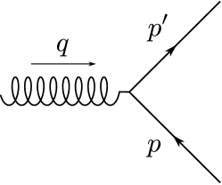
(a) Tree Level

(b) Self Energy

(c) Counter Term

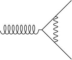
(d) Electromagnetic Vertex

(e) Contact

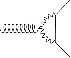
(f) Photon Polarization

Figure 2: The diagrams contributing to the radiative corrections to the stress-energy tensor. The curly line is the stress-energy tensor, the wavy line is the photon and the solid line is the fermion.

In order to evaluate the radiative corrections to gravitomagnetic moment at finite temperature we have to consider the renormalization of the stress-energy tensor at finite temperature and at first order on momentum transfer $q$. The zero temperature renormalization is performed with usual techniques and we do not discuss it here. To address thermal corrections to the matrix-element of stress-energy tensor we use the real-time formalism of thermal field theory. The major modification of QFT at finite temperature is the value of the vacuum of the theory, which is not empty but contain a number of bosons and fermions given respectively by the Bose-Einstein and the Fermi-Dirac distribution functions:

$$\widehat{a}_{\textup{B}}^{\dagger}\widehat{a}_{\textup{B}}(p)|0\rangle=n_{\textup{B}}(E)|0\rangle,\quad\widehat{a}_{\textup{F}}^{\dagger}\widehat{a}_{\textup{F}}(p)|0\rangle=n_{\textup{F}}(E)|0\rangle,$$

where as usual we indicate

$$n_{\textup{B}}(x)=\frac{1}{\exp(\beta x)-1},\quad n_{\textup{F}}(x)=\frac{1}{\exp(\beta x)+1}.$$

The resulting propagators of the gauge field and of the fermionic field in real-time formalism are

$$\begin{split}\mathrm{i}S_{F}(p)&=\left(\not{p}+m\right)\left[\frac{\mathrm{i}}{p^{2}-m^{2}}-2\pi\delta\left(p^{2}-m^{2}\right)n_{F}(p)\right],\\ \mathrm{i}D_{\mu\nu}(k)&=-\eta_{\mu\nu}\left[\frac{\mathrm{i}}{k^{2}}+2\pi\delta\left(k^{2}\right)n_{B}(k)\right].\end{split}$$

Perturbation theory and Feynman diagrams at finite temperature are unmodified compared to usual quantum field theory except for the previous propagators. We see that the propagators in real-time formalism are naturally separated into a temperature part and into a $T=0$ part. The $T=0$ part has been addressed as usual and from now on we just consider the thermal part. The diagrams responsible for radiative corrections to the stress-energy tensor matrix element

$$\langle p^{\prime},s^{\prime}|T^{\mu\nu}(0)|p,s\rangle=\frac{1}{\sqrt{Z_{2}(p)Z_{2}(p^{\prime})}}\bar{u}_{\beta}(p^{\prime})M_{\mu\nu}(p,p^{\prime})u_{\beta}(p),$$

are reported in Fig. 2. Furthermore, since we are only interested in the thermal part, each integrals corresponding to a Feynman diagram is weighted with a thermal function and it is therefore ultraviolet convergent and finite. All the divergent part are already been taken care of with the $T=0$ renormalization.

Note that we can distinguish between two different regimes of temperature. Indeed, finite-temperature modification may arise both from the boson or the photon propagators. However, for low temperatures such that $T\ll m$, the fermion distribution function is suppressed by a factor $\exp(-m/T)$, which is negligible compared to contributions of order $(T/m)^{2}$ coming from the photon distribution. In the opposite regime, when $T\gg m$, the photon contribution is still the same as low temperatures, while the fermion distribution can now also contribute with terms of order $(T/m)^{2}$. Therefore, as in the case of the pole of the propagator, we can expect two different values of AGM valid in the two regimes of low and high temperatures.

As first step, we need to identify the mass shift and the wave-function renormalization constant. These quantities are obtained starting from the self-energy of the fermion, which is discussed in Sec. A.1. We found that the self-energy can be written as $\Sigma(p)=a\not{p}+b\not{u}+c$ and that the full fermion propagator becomes

$$S(p)=\frac{(1-a)\not{p}-b\not{u}+m+c}{[(1-a)p-bu]^{2}-(m+c)^{2}},$$ (30)

which has a pole in $\omega^{2}=E_{\beta}^{2}=p_{s}^{2}+m_{p}^{2}$, with $m_{p}$ given by Eq. (27).

C.1 Thermal Dirac spinor

The Dirac equation in momentum space is modified according to the self-energy, which also include thermal modifications. The thermal Dirac spinors $u_{\beta}(p)$ satisfy the modified Dirac equation corresponding to the new propagator (30):

$$\left[\not{p}-m_{R}-\Sigma^{\beta}(p)\right]u_{\beta}(p)=\left[(1-a)\not{p}-b\not{u}-m_{R}-c\right]u_{\beta}(p)=0,$$

where $m_{R}$ indicates the zero temperature renormalized mass. The thermal spinor $u_{\beta}(p)$ satisfies the previous equation when $p$ is the pole of the propagator, i.e. such that $p\cdot u=E_{\beta}(p_{s})$. The thermal Dirac spinors are actually required to properly account for stress-energy tensor renormalization at finite temperature Donoghue et al. (1984); Weldon (1982b).

In thermal bath rest frame, we choose the normalization

$$u^{\dagger}_{\beta}(p)u_{\beta}(p)=1.$$

For convenience, we furthermore define a four vector and a scalar

$$p_{T}\equiv(1-a)p-bu,\quad m_{T}\equiv m_{R}+c,$$

so that the modified thermal Dirac equation is written as

$$\left[\not{p}_{T}-m_{T}\right]u_{\beta}(p)=0.$$

Therefore, it follows from the modified thermal Dirac equation that the thermal spinors satisfy the following identities:

$$\bar{u}_{\beta}(p,s)u_{\beta}(p,s)=\frac{m_{T}}{(1-a)E_{\beta}-b},\quad\bar{u}_{\beta}(p,s)\gamma_{\mu}u_{\beta}(p,s)=\frac{{p_{T}}_{\mu}}{(1-a)E_{\beta}-b},\quad\sum_{s}u_{\beta}(p,s)\bar{u}_{\beta}(p,s)=\frac{\not{p}_{T}+m_{T}}{2(1-a)E_{\beta}-2b}.$$

In the non relativistic limit and in the frame where $u=(1,\mathchoice{\mbox{\boldmath$\displaystyle\mathbf{0}$}}{\mbox{\boldmath$\textstyle\mathbf{0}$}}{\mbox{\boldmath$\scriptstyle\mathbf{0}$}}{\mbox{\boldmath$\scriptscriptstyle\mathbf{0}$}})$, we can also show the validity of the following identities:

$$\bar{u}_{\beta}(p^{\prime})\gamma_{0}u_{\beta}(p)=\xi^{\prime\dagger}\xi+\mathcal{O}(e^{2}),\quad\bar{u}_{\beta}(p^{\prime})\mathchoice{\mbox{\boldmath$\displaystyle\mathbf{\gamma}$}}{\mbox{\boldmath$\textstyle\mathbf{\gamma}$}}{\mbox{\boldmath$\scriptstyle\mathbf{\gamma}$}}{\mbox{\boldmath$\scriptscriptstyle\mathbf{\gamma}$}}u_{\beta}(p)=\xi^{\prime\dagger}\left[\frac{\mathchoice{\mbox{\boldmath$\displaystyle\mathbf{P}$}}{\mbox{\boldmath$\textstyle\mathbf{P}$}}{\mbox{\boldmath$\scriptstyle\mathbf{P}$}}{\mbox{\boldmath$\scriptscriptstyle\mathbf{P}$}}}{2m_{p}}+\mathrm{i}\frac{\mathchoice{\mbox{\boldmath$\displaystyle\mathbf{\sigma}$}}{\mbox{\boldmath$\textstyle\mathbf{\sigma}$}}{\mbox{\boldmath$\scriptstyle\mathbf{\sigma}$}}{\mbox{\boldmath$\scriptscriptstyle\mathbf{\sigma}$}}\wedge\mathchoice{\mbox{\boldmath$\displaystyle\mathbf{q}$}}{\mbox{\boldmath$\textstyle\mathbf{q}$}}{\mbox{\boldmath$\scriptstyle\mathbf{q}$}}{\mbox{\boldmath$\scriptscriptstyle\mathbf{q}$}}}{2m_{p}}\right]\xi+\mathcal{O}(e^{4}),$$

where $\xi$ is the two component spinor, normalized such that $\xi^{\dagger}\xi=1$. We used the identities above to compute the gravitational mass in Sec. A.3 and the gravitomagnetic moment in Sec. IV.

C.2 Wave-function renormalization constant $Z_{2}$

The wave-function renormalization constant $Z_{2}$ is obtained by requesting that the fermion field is properly renormalized

$$\psi_{\textup{R}}(x)=\frac{1}{\sqrt{Z_{2}}}\psi_{0}(x).$$

The temperature part of the wave-function renormalization constant is Donoghue and Holstein (1983); Mitra et al. (2001)

$${}^{\beta}Z_{2}(\omega,p_{s})=\frac{2\left[(1-a)E_{\beta}-b\right]}{\frac{\partial D}{\partial\omega}\Big{|}_{\omega=E_{\beta}}},$$

where $E_{\beta}$ is the pole of the propagator and $D$ is the denominator of the propagator (30)

$$D(\omega,p_{s})=(1-a)^{2}(\omega^{2}-p_{s}^{2})+b^{2}-2(1-a)b\omega-(m+c)^{2}.$$

At order $e^{2}$ we find

$$^{\beta}Z_{2}=1+\left(a+\frac{m^{2}}{\omega}\frac{\partial a}{\partial\omega}+\frac{\partial b}{\partial\omega}+\frac{m}{\omega}\frac{\partial c}{\partial\omega}\right)\Big{|}_{\omega=\sqrt{p_{s}^{2}+m^{2}}}.$$ (31)

For the computation of AGM we are interested to the quantity $(\sqrt{Z_{2}(p)Z_{2}(p^{\prime})})^{-1/2}$ in the limits of $q\to 0$ and of $P_{s}=\sqrt{(P\cdot u)^{2}-P^{2}}\to 0$. Therefore, we just have to evaluate $Z_{2}(p)$ with $p$ an on-shell momentum and then perform the $p_{s}\to 0$ limit. Using the prescription in Eq. (31) and the behavior of the functions $a,b,c$ we find:

$$\lim_{p_{s}\to 0}\,^{\beta}Z_{2}(p)=1-\frac{e^{2}T^{2}}{12m^{2}}+\frac{e^{2}}{2\pi^{2}}\int_{0}^{\infty}{\rm d}k\,\frac{n_{\textup{B}}(k)}{k}-\theta_{\textup{HT}}\frac{e^{2}T^{2}}{24m^{2}},$$

where the $\theta_{\textup{HT}}$ is defined such that it turns on the high temperatures contribution:

$$\theta_{\textup{HT}}\equiv\begin{cases}0&T\ll m\\ 1&T\gg m\end{cases}.$$

The low-temperature part is in agreement with Donoghue and Holstein (1983); Donoghue et al. (1984); Mitra et al. (2001). Therefore we have

$$\lim_{p_{s}\to 0}\frac{1}{\sqrt{\,{}^{\beta}Z_{2}(p)\,^{\beta}Z_{2}(p^{\prime})}}=1+\frac{e^{2}T^{2}}{12m^{2}}-\frac{e^{2}}{16\pi^{3}}I_{\textup{A}}+\theta_{\textup{HT}}\,\frac{e^{2}T^{2}}{24m^{2}},$$

where we denoted

$$I_{\textup{A}}\equiv 8\pi\int_{0}^{\infty}{\rm d}k\,\frac{n_{\textup{B}}(k)}{k}.$$

For future convenience, noticing that for $p_{s}=0$ we have $\omega_{P}=2m$, we can write the factor coming from wave-function renormalization constants using $\omega_{P}\equiv u\cdot P$ instead of the mass $m$:

$$\lim_{P_{s}\to 0}\lim_{q\to 0}\frac{1}{\sqrt{\,{}^{\beta}Z_{2}(p)\,^{\beta}Z_{2}(p^{\prime})}}=1+\frac{e^{2}T^{2}}{3\omega_{P}^{2}}-\frac{e^{2}}{16\pi^{3}}I_{\textup{A}}+\theta_{\textup{HT}}\,\frac{e^{2}T^{2}}{6\omega_{P}^{2}}.$$

C.3 Renormalization of stress-energy tensor at finite temperature

As last step to renormalize the stress-energy tensor we have to calculate the temperature contribution of the diagrams in Fig. 2. Here we write the general procedure and we leave the details in Appendix D.

First, we recap the notation used. We indicate with $q$ and $P$ the momenta

$$P=p^{\prime}+p,\quad q=p^{\prime}-p$$

where $p$ and $p^{\prime}$ are the momenta of external legs of the diagrams in Fig. 2. Notice that $q\cdot P=0$. Moreover, scattering theory imposes the conservation of the time component of $p$ and $p^{\prime}$ in the thermal bath rest frame, meaning $q\cdot u=0$. We are using this constraint when evaluating all the diagrams. It is then convenient to define the following scalar and four-vectors:

$$\omega_{P}=P\cdot u,\quad P_{s}=\sqrt{\omega_{P}^{2}-P^{2}},\quad\tilde{P}_{\mu}=(\eta_{\mu\nu}-u_{\mu}u_{\nu})P^{\nu}=P_{\mu}-\omega_{P}u_{\mu},\quad l^{\mu}=\epsilon^{\mu\nu\rho\sigma}u_{\nu}\tilde{P}_{\rho}q_{\sigma},\quad\hat{l}^{\mu}=\frac{l^{\mu}}{\sqrt{-l^{2}}},$$

we also denote with $a$ the ratio

$$a\equiv\frac{\sqrt{\omega_{P}^{2}-P^{2}}}{\omega_{P}}=\frac{P_{s}}{\omega_{P}},\quad 0<a<1.$$

Since we are considering 1-loop corrections, a generic diagrams of Fig. 2, which we label with $X$, can be written as

$$M_{\mu\nu}^{X}(p,p^{\prime})=\int\frac{{\rm d}^{4}k}{(2\pi)^{4}}\frac{f^{X}(p,p^{\prime},k)}{D^{X}(p,p^{\prime},k)}\bar{u}(p^{\prime})N^{X}_{\mu\nu}u(p),$$ (32)

where all the spinorial structure is contained inside the numerator $N^{X}$. Therefore $N^{X}$ can be simplified using Dirac equation and it can be decomposed in the following terms:

$$\begin{split}\bar{u}(p^{\prime})N^{X}_{\mu\nu}u(p)=&\bar{u}(p^{\prime})\Big{[}N_{kk}^{X}\not{k}\,k_{\mu}k_{\nu}+N_{Pk}^{X}\not{k}\,(P_{\mu}k_{\nu}+P_{\nu}k_{\mu})+\\ &+(N_{P\gamma}^{X(s)}+N_{P\gamma}^{X(k)}\not{k})(P_{\mu}\gamma_{\nu}+P_{\nu}\gamma_{\mu})+(N_{k\gamma}^{X(s)}+N_{k\gamma}^{X(k)}\not{k})(k_{\mu}\gamma_{\nu}+k_{\nu}\gamma_{\mu})+\cdots\Big{]}u(p)\end{split}$$ (33)

where each term $N_{yy}^{X}$ can depend on the scalars $\{k^{2},\,P^{2},\,q^{2},k\cdot P,\,k\cdot q,\,P\cdot q,\,m\}$ and the dots stands for terms that to do not contribute to AGM. Indeed, we show in App. B that the only terms that are relevant for AGM are

$$\begin{split}u_{\mu}\gamma_{\nu}+u_{\nu}\gamma_{\mu},&\quad P_{\mu}\gamma_{\nu}+P_{\nu}\gamma_{\mu},\quad\not{\hat{l}}\left(u_{\mu}\hat{l}_{\nu}+u_{\nu}\hat{l}_{\mu}\right),\quad\not{\hat{l}}\left(P_{\mu}\hat{l}_{\nu}+P_{\nu}\hat{l}_{\mu}\right).\end{split}$$

Using the orthogonal non-normalized basis $\{u,\,\tilde{P},\,q,\,\hat{l}\}$, the integration variable $k$ can be decomposed into:

$$\begin{split}k_{\mu}=&(k\cdot u)u_{\mu}+\frac{(k\cdot\tilde{P})}{\tilde{P}^{2}}\tilde{P}_{\mu}+\frac{(k\cdot q)}{q^{2}}q_{\mu}-(k\cdot\hat{l})\hat{l}_{\mu}\\ =&\left[(k\cdot u)-\frac{\omega_{P}(k\cdot\tilde{P})}{\tilde{P}^{2}}\right]u_{\mu}+\frac{(k\cdot\tilde{P})}{\tilde{P}^{2}}P_{\mu}+\frac{(k\cdot q)}{q^{2}}q_{\mu}-(k\cdot\hat{l})\hat{l}_{\mu}\\ \equiv&A_{u}\,u_{\mu}+A_{P}\,P_{\mu}+A_{q}\,q_{\mu}+A_{l}\,\hat{l}_{\mu}.\end{split}$$

This decomposition is used to write the diagrams in a covariant form. Consider the term $\bar{u}(p^{\prime})\not{k}u(p)v_{\mu}w_{\mu}$, where $v$ and $w$ are any vector between $\{u,P,q,l\}$, the term is decomposed into

$$\bar{u}(p^{\prime})\not{k}u(p)v_{\mu}w_{\nu}=\bar{u}(p^{\prime})\left[A_{u}\,\not{u}+A_{l}\,\not{\hat{l}}+2mA_{P}\right]u(p)v_{\mu}w_{\nu},$$

and for what we show in Sec. IV.2 only the term in $\not{l}$ can contribute to AGM:

$$\bar{u}(p^{\prime})\not{k}u(p)v_{\mu}w_{\nu}\to A_{l}\,\bar{u}(p^{\prime})\,\not{\hat{l}}\,v_{\mu}w_{\nu}\,u(p)\quad\text{ with }(v,w)=(u,l)\text{ or }(v,w)=(P,l).$$

With the same argument, we can select only the parts relevant to AGM of all the possible terms:

$$\begin{split}\bar{u}(p^{\prime})\not{k}u(p)\left(k_{\mu}v_{\nu}+k_{\nu}v_{\mu}\right)\to&\bar{u}(p^{\prime})\Big{[}A_{u}A_{l}\not{\hat{l}}(u_{\mu}v_{\nu}+u_{\nu}v_{\mu})+A_{P}A_{l}\not{\hat{l}}(P_{\mu}v_{\nu}+P_{\nu}v_{\mu})\Big{]}u(p)\text{ if }v=l\\ \to&\bar{u}(p^{\prime})\Big{[}A_{l}^{2}\not{\hat{l}}(\hat{l}_{\mu}v_{\nu}+\hat{l}_{\nu}v_{\mu})\Big{]}u(p)\text{ if }v=u\text{ or }v=P\\ \bar{u}(p^{\prime})\not{k}k_{\mu}k_{\nu}u(p)\to&\bar{u}(p^{\prime})\Big{[}A_{u}A_{l}^{2}\,\not{\hat{l}}(u_{\mu}\hat{l}_{\nu}+u_{\nu}\hat{l}_{\mu})+A_{P}A_{l}^{2}\,\not{\hat{l}}(P_{\mu}\hat{l}_{\nu}+P_{\nu}\hat{l}_{\mu})\Big{]}u(p).\end{split}$$

We then approximate the integrand to first order in $q$ and we perform the loop integral in $k$ decomposing its component along the tetrad $\{u,\tilde{P},q,l\}$. The results at first order in $q$ are (see Appendix D):

$$\begin{split}(Z_{2}(p)Z_{2}(p^{\prime}))^{-1/2}M_{\mu\nu}^{(0)}=&I^{Z}_{P\gamma}\left(P_{\mu}\gamma_{\nu}+P_{\nu}\gamma_{\mu}\right),\\ M_{\mu\nu}^{SE}+M_{\mu\nu}^{CT}=&I^{S}_{P\gamma}\left(P_{\mu}\gamma_{\nu}+P_{\nu}\gamma_{\mu}\right),\\ M_{\mu\nu}^{V}=&\left(I^{V}_{P\gamma}+\theta_{\textup{HT}}I^{V}_{P\gamma,f}\right)\left(P_{\mu}\gamma_{\nu}+P_{\nu}\gamma_{\mu}\right)+\left(I^{V}_{u\gamma}+\theta_{\textup{HT}}I^{V}_{u\gamma,f}\right)\left(u_{\mu}\gamma_{\nu}+u_{\nu}\gamma_{\mu}\right)\\ &+\left(I^{V}_{Pl}+\theta_{\textup{HT}}I^{V}_{Pl,f}\right)\not{\hat{l}}\left(P_{\mu}\hat{l}_{\nu}+P_{\nu}\hat{l}_{\mu}\right)+\theta_{\textup{HT}}I^{V}_{ul,f}\not{\hat{l}}\left(u_{\mu}\hat{l}_{\nu}+u_{\nu}\hat{l}_{\mu}\right),\\ M_{\mu\nu}^{C}=&\left(I^{C}_{P\gamma}+\theta_{\textup{HT}}I^{C}_{P\gamma,f}\right)\left(P_{\mu}\gamma_{\nu}+P_{\nu}\gamma_{\mu}\right)+\left(I^{C}_{u\gamma}+\theta_{\textup{HT}}I^{C}_{u\gamma,f}\right)\left(u_{\mu}\gamma_{\nu}+u_{\nu}\gamma_{\mu}\right),\\ M_{\mu\nu}^{P}=&I^{P}_{P\gamma}\left(P_{\mu}\gamma_{\nu}+P_{\nu}\gamma_{\mu}\right)+I^{P}_{u\gamma}\left(u_{\mu}\gamma_{\nu}+u_{\nu}\gamma_{\mu}\right)+\left(I^{P}_{Pl}+\theta_{\textup{HT}}I^{P}_{Pl,f}\right)\not{\hat{l}}\left(P_{\mu}\hat{l}_{\nu}+P_{\nu}\hat{l}_{\mu}\right)\\ &+\left(I^{P}_{ul}+\theta_{\textup{HT}}I^{P}_{ul,f}\right)\not{\hat{l}}\left(u_{\mu}\hat{l}_{\nu}+u_{\nu}\hat{l}_{\mu}\right).\end{split}$$

Here, the function

$$\theta_{\textup{HT}}\equiv\begin{cases}0&T\ll m\\ 1&T\gg m\end{cases}$$

turns on the fermionic contributions at high temperature and removes them for low temperatures; we also introduce the IR divergent integral

$$I_{\textup{A}}\equiv 8\pi\int_{0}^{\infty}{\rm d}k\frac{n_{\textup{B}}(k)}{k}.$$

The form factors of $P_{\mu}\gamma_{\nu}+P_{\nu}\gamma_{\mu}$ are

$$\begin{split}\lim_{P_{s}\to 0}\lim_{q\to 0}I^{Z}_{P\gamma}=&\frac{1}{4}+\frac{2+\theta_{\textup{HT}}}{24}\frac{e^{2}T^{2}}{\omega_{P}^{2}}-\frac{1}{4}\frac{e^{2}}{16\pi^{3}}I_{\textup{A}};\\ \lim_{P_{s}\to 0}\lim_{q\to 0}I^{S}_{P\gamma}=&-\frac{2+\theta_{\textup{HT}}}{12}\frac{e^{2}T^{2}}{\omega_{P}^{2}}+\frac{1}{2}\frac{e^{2}}{16\pi^{3}}I_{\textup{A}};\\ I^{V}_{P\gamma}=&-\frac{1}{18}\frac{e^{2}T^{2}}{\omega_{P}^{2}}\left[\frac{3}{2a^{3}}\log\left(\frac{1+a}{1-a}\right)-\frac{3}{a^{2}}\right]-\frac{1}{4}\frac{e^{2}}{16\pi^{3}}\frac{4m^{2}}{\omega_{P}^{2}}\frac{I_{A}}{1-a^{2}};\\ I^{V}_{P\gamma,f}=&-\frac{1}{36}\frac{e^{2}T^{2}}{\omega_{P}^{2}}\left[\frac{3}{2a^{3}}\log\left(\frac{1+a}{1-a}\right)-\frac{3}{a^{2}}\right];\\ I^{C}_{P\gamma}=&\frac{1}{18}\frac{e^{2}T^{2}}{\omega_{P}^{2}}\left[\frac{3}{2a^{3}}\log\left(\frac{1+a}{1-a}\right)-\frac{3}{a^{2}}\right];\\ I^{C}_{P\gamma,f}=&\frac{1}{36}\frac{e^{2}T^{2}}{\omega_{P}^{2}}\left[\frac{3}{2a^{3}}\log\left(\frac{1+a}{1-a}\right)-\frac{3}{a^{2}}\right];\\ I^{P}_{P\gamma}=&-\frac{1}{18}\frac{e^{2}T^{2}}{\omega_{P}^{2}}\left[\frac{3}{2a^{3}}\log\left(\frac{1+a}{1-a}\right)-\frac{3}{a^{2}}\right].\end{split}$$

The form factors of $u_{\mu}\gamma_{\nu}+u_{\nu}\gamma_{\mu}$ are

$$\begin{split}I^{V}_{u\gamma}=&-\frac{1}{9}\frac{e^{2}T^{2}}{\omega_{P}}\left[\frac{3}{2a^{3}}\log\left(\frac{1+a}{1-a}\right)-\frac{3}{a^{2}}\right];\\ I^{V}_{u\gamma,f}=&-\frac{1}{18}\frac{e^{2}T^{2}}{\omega_{P}}\left[\frac{3}{2a^{2}}-\frac{3(1-a^{2})}{4a^{3}}\log\left(\frac{1+a}{1-a}\right)\right];\\ I^{C}_{u\gamma}=&\frac{1}{9}\frac{e^{2}T^{2}}{\omega_{P}}\left[\frac{3}{2a^{2}}-\frac{3(1-a^{2})}{4a^{3}}\log\left(\frac{1+a}{1-a}\right)\right];\\ I^{C}_{u\gamma,f}=&\frac{1}{18}\frac{e^{2}T^{2}}{\omega_{P}}\left[\frac{3}{2a^{2}}-\frac{3(1-a^{2})}{4a^{3}}\log\left(\frac{1+a}{1-a}\right)\right];\\ I^{P}_{u\gamma}=&-\frac{1}{9}\frac{e^{2}T^{2}}{\omega_{P}}\left[\frac{3}{2a^{2}}-\frac{3(1-a^{2})}{4a^{3}}\log\left(\frac{1+a}{1-a}\right)\right].\end{split}$$

The form factors of $\not{\hat{l}}(P_{\mu}\hat{l}_{\nu}+P_{\nu}\hat{l}_{\mu})$ are

$$\begin{split}I^{V}_{Pl}=&\frac{1}{12}\frac{e^{2}T^{2}}{\omega_{P}^{2}}\left[\frac{3}{2a^{3}}\log\left(\frac{1+a}{1-a}\right)-\frac{3}{a^{2}}\right];\\ I^{V}_{Pl,f}=&\frac{7}{360}\frac{e^{2}T^{2}}{\omega_{P}^{2}}\left[\frac{12}{7}\frac{4m^{2}}{\omega_{P}^{2}}\left(\frac{5(3-2a^{2})}{2a^{4}(1-a^{2})}-\frac{15}{4a^{5}}\log\left(\frac{1+a}{1-a}\right)\right)-\frac{5}{7}\left(\frac{3}{2a^{3}}\log\left(\frac{1+a}{1-a}\right)-\frac{3}{a^{2}}\right)\right];\\ I^{P}_{Pl}=&I^{P}_{P\gamma}=-\frac{1}{18}\frac{e^{2}T^{2}}{\omega_{P}^{2}}\left[\frac{3}{2a^{3}}\log\left(\frac{1+a}{1-a}\right)-\frac{3}{a^{2}}\right];\\ I^{P}_{Pl,f}=&-\frac{1}{30}\frac{e^{2}T^{2}}{\omega_{P}^{2}}\frac{4m^{2}}{\omega_{P}^{2}}\left[\frac{15(3-a^{2})}{8a^{5}}\log\left(\frac{1+a}{1-a}\right)-\frac{45}{4a^{4}}\right].\end{split}$$

The form factors of $\not{\hat{l}}(u_{\mu}\hat{l}_{\nu}+u_{\nu}\hat{l}_{\mu})$ are

$$\begin{split}I^{V}_{ul,f}=&-\frac{1}{30}\frac{e^{2}T^{2}}{\omega_{P}}\left[-\frac{2}{3}\frac{4m^{2}}{\omega_{P}^{2}}\left(\frac{15(3-2a^{2})}{8a^{5}}\log\left(\frac{1+a}{1-a}\right)-\frac{45}{4a^{4}}\right)+\frac{5}{3}\left(\frac{3}{2a^{2}}-\frac{3(1-a^{2})}{4a^{3}}\log\left(\frac{1+a}{1-a}\right)\right)\right];\\ I^{P}_{ul}=&I^{P}_{u\gamma}=-\frac{1}{9}\frac{e^{2}T^{2}}{\omega_{P}}\left[\frac{3}{2a^{2}}-\frac{3(1-a^{2})}{4a^{3}}\log\left(\frac{1+a}{1-a}\right)\right];\\ I^{P}_{ul,f}=&-\frac{1}{45}\frac{e^{2}T^{2}}{\omega_{P}}\frac{4m^{2}}{\omega_{P}^{2}}\left[\frac{15(3-a^{2})}{8a^{5}}\log\left(\frac{1+a}{1-a}\right)-\frac{45}{4a^{4}}\right].\end{split}$$

These functions are written such that the quantity inside the square brackets is 1 for $a=0$, which correspond to the non relativistic particle limit ($P_{s}\to 0$). It is straightforward to check that by summing all these terms in the non-relativistic limit, one get the form factors quoted in Eq. (21).

Appendix D Radiative correction to the stress-energy tensor

In this appendix we evaluate the temperature modification of the diagrams in Fig. 2. The general strategy and the final results are written in Sec. C.3, in what follows we provide a detailed calculations of all the diagrams.

To perform the loop integration on the momentum $k$ in the generic diagram (32), since the set $\{u,\,\tilde{P},\,q,\,\hat{l}\}$ is a basis, we choose $k_{0}$ along $u$, $k_{z}$ along $q_{\mu}$ and $k_{x}$ along $\tilde{P}$ and $k_{y}$ along $l$; thus, defining

$$\epsilon=\sqrt{-q^{2}},\quad a=\frac{\sqrt{-\tilde{P}^{2}}}{\omega_{P}}=\frac{\sqrt{\omega_{P}^{2}-P^{2}}}{\omega_{P}},\quad 0<a<1,$$

we have

$$\begin{split}(k\cdot u)&=k_{0},\quad(k\cdot q)=-\epsilon\,k_{z},\quad(k\cdot\tilde{P})=-a\omega_{P}\,k_{x}\quad(k\cdot P)=\omega_{P}(k_{0}-ak_{x}),\quad(k\cdot\hat{l})=-k_{y}\\ A_{u}&=k_{0}-\frac{k_{x}}{a},\quad A_{P}=\frac{k_{x}}{a\omega_{P}},\quad A_{q}=\frac{k_{z}}{\epsilon},\quad A_{l}=k_{y}.\end{split}$$

At last we define the following unit vectors inside the $k$ integration:

$$\hat{k}_{x}=\frac{k_{x}}{|\mathchoice{\mbox{\boldmath$\displaystyle\mathbf{k}$}}{\mbox{\boldmath$\textstyle\mathbf{k}$}}{\mbox{\boldmath$\scriptstyle\mathbf{k}$}}{\mbox{\boldmath$\scriptscriptstyle\mathbf{k}$}}|}=\cos\phi\sin\theta,\quad\hat{k}_{y}=\frac{k_{y}}{|\mathchoice{\mbox{\boldmath$\displaystyle\mathbf{k}$}}{\mbox{\boldmath$\textstyle\mathbf{k}$}}{\mbox{\boldmath$\scriptstyle\mathbf{k}$}}{\mbox{\boldmath$\scriptscriptstyle\mathbf{k}$}}|}=\sin\phi\sin\theta,\quad\hat{k}_{z}=\frac{k_{z}}{|\mathchoice{\mbox{\boldmath$\displaystyle\mathbf{k}$}}{\mbox{\boldmath$\textstyle\mathbf{k}$}}{\mbox{\boldmath$\scriptstyle\mathbf{k}$}}{\mbox{\boldmath$\scriptscriptstyle\mathbf{k}$}}|}=\cos\theta.$$

For the fermionic part we only consider the high temperature limit, $T\gg m,P_{s},\omega_{p},q$. Every fermionic form factor at first order in $\epsilon$ can be written as

$$I=C\int\frac{{\rm d}k}{E_{k}}k^{l}n_{\textup{F}}(E_{k})\sum_{s=\pm}\int{\rm d}\Omega_{k}f_{s}(\hat{k},m,\omega_{p},a),$$

where $C$ is a numerical constant and $l$ an integer. Because of the Fermi-Dirac distribution function, the major contribution of the integral comes from $k\sim T$. Then in the integrand we can consider $m$ and $\omega_{P}$ to be small compared to $k$. To consider the relevant part of the integral we first replace

$$m=m_{r}ky,\quad\omega_{P}=\omega_{Pr}ky,\quad E_{k}=k\sqrt{1+m_{r}^{2}y^{2}},$$

where $y$ is a dummy variable to perform a Taylor series. Then we expand the integrand in series of $y$ around zero and we keep only the first terms. Then we replace back

$$y=1,\quad m_{r}=\frac{m}{k},\quad\omega_{Pr}=\frac{\omega_{P}}{k}.$$

In this way we can select the relevant contribution, which has the form

$$I\simeq C\int{\rm d}k\,n_{\textup{F}}(E_{k})\sum_{s=\pm}\int{\rm d}\Omega_{k}\tilde{f}_{s}(\hat{k},m,\omega_{p},a)=\frac{C\pi^{2}T^{2}}{12}\sum_{s=\pm}\int{\rm d}\Omega_{k}\tilde{f}_{s}(\hat{k},m,\omega_{p},a).$$

The last factor can be obtained by summing and integrating over the angles. The angular integrals have the form

$$I_{\Omega}(n_{x},n_{y},n_{z},n_{d})=\int{\rm d}\Omega_{k}\frac{2\hat{k}_{x}^{n_{x}}\hat{k}_{y}^{n_{y}}\hat{k}_{z}^{n_{z}}}{(1-a^{2}\hat{k}_{x}^{2})^{n_{d}}}$$

and their results are quoted in Sec. D.5.

D.1 Self-energy and Counter-terms

The fermion-self energy diagram, Fig. 2(b), is

$$M_{\mu\nu}^{SE}=\bar{u}(p^{\prime})\,^{\beta}\Sigma(p^{\prime})\mathrm{i}S_{F}(p^{\prime})V_{\mu\nu}(p^{\prime},p)u(p),$$

where $V_{\mu\nu}$ is the stress-energy tensor fermion coupling:

$$V_{\mu\nu}(p,p^{\prime})=\frac{1}{4}\left[\gamma_{\mu}(p+p^{\prime})_{\nu}+\gamma_{\nu}(p+p^{\prime})_{\mu}\right]-\frac{1}{2}\eta_{\mu\nu}\left[\not{p}-m+\not{p}^{\prime}-m\right].$$

Near the pole the self-energy can be written as

$${}^{\beta}\Sigma(p)=\left(1-\,^{\beta}Z_{2}(p)^{-1}\right)\left(\not{p}-m\right)+a\not{p}+b\not{u}+\delta m.$$

Most of this diagram is canceled by the counter-term in Fig. 2(c). Since the temperature dependent Dirac equation is

$$\left((1-a)\not{p}-b\not{u}-m_{\textup{T}}\right)u_{\beta}(p)=0,$$

we must use the finite temperature counter-term of the momentum Lagrangian

$$\delta\mathcal{L}=a\not{p}+b\not{u}+\delta m.$$

Therefore, the counter term is

$$\begin{split}M_{\mu\nu}^{CT}=&-\bar{u}(p^{\prime})\,\left(a\not{p^{\prime}}+b\not{u}+\delta m\right)\mathrm{i}S_{F}(p^{\prime})V_{\mu\nu}(p^{\prime},p)u(p).\end{split}$$

Considering both legs we have in total

$$\begin{split}M_{\mu\nu}^{SE}+M_{\mu\nu}^{CT}=&\left(2-\,^{\beta}Z_{2}(p)^{-1}-\,^{\beta}Z_{2}(p^{\prime})^{-1}\right)\bar{u}(p^{\prime})V_{\mu\nu}(p^{\prime},p)u(p),\end{split}$$

whose contribution to AGM is

$$\begin{split}M_{\mu\nu}^{SE}+M_{\mu\nu}^{CT}=&\frac{1}{4}\left(2-\,^{\beta}Z_{2}(p)^{-1}-\,^{\beta}Z_{2}(p^{\prime})^{-1}\right)\bar{u}(p^{\prime})\left(P_{\mu}\gamma_{\nu}+P_{\nu}\gamma_{\mu}\right)u(p)\\ =&I^{S}_{P\gamma}\bar{u}(p^{\prime})\left(P_{\mu}\gamma_{\nu}+P_{\nu}\gamma_{\mu}\right)u(p).\end{split}$$

In the limit $q\to 0$ and $P_{s}\to 0$ we have

$$\lim_{P_{s}\to 0}I^{S}_{P\gamma}=-\frac{e^{2}T^{2}}{6\omega_{P}^{2}}+\frac{1}{2}\frac{e^{2}}{16\pi^{3}}I_{\textup{A}}-\theta_{\textup{HT}}\,\frac{e^{2}T^{2}}{12\omega_{P}^{2}},$$

where $\theta_{\textup{HT}}$ is vanishing for $T\ll m$ and it goes to one for $T\gg m$.

D.2 Photon polarization diagram

Now we want to check if gravitomagnetic moment gets finite temperature corrections from the diagram of photon polarization Fig. 2(f):

$$M^{P}_{\mu\nu}(p,p^{\prime})=\int\frac{{\rm d}^{4}k}{(2\pi)^{4}}\bar{u}(p^{\prime})(-\mathrm{i}e\gamma_{\rho})\mathrm{i}S_{F}(p-k)(-\mathrm{i}e\gamma_{\sigma})u(p)T^{\alpha\beta}_{\mu\nu}(k,q+k)\mathrm{i}D^{\rho}_{\beta}(q+k)\mathrm{i}D^{\sigma}_{\alpha}(k)$$

where the stress-energy tensor-photon coupling vertex is

$$\begin{split}T^{\alpha\beta}_{\mu\nu}(k,p)=&-(\delta^{\alpha}_{\mu}\delta^{\beta}_{\nu}+\delta^{\alpha}_{\nu}\delta^{\beta}_{\mu})k\cdot p-g^{\alpha\beta}(k_{\mu}p_{\nu}+k_{\nu}p_{\mu})+(k_{\mu}\delta^{\beta}_{\nu}+k_{\nu}\delta^{\beta}_{\mu})p^{\alpha}+\\ &+(p_{\mu}\delta^{\alpha}_{\nu}+p_{\nu}\delta^{\alpha}_{\mu})k^{\beta}+g_{\mu\nu}(\delta^{\alpha\beta}k\cdot p-k^{\alpha}p^{\beta}).\end{split}$$

At low temperature $T\ll m$ we can neglect the part coming from the fermionic thermal distribution. The real part of the thermal contribution of the diagram is then

$$\begin{split}\text{Re}^{\beta}M^{P}_{\mu\nu}(p,p^{\prime})=&e^{2}\int\frac{{\rm d}^{4}k}{(2\pi)^{3}}\bar{u}(p^{\prime})\gamma_{\alpha}\,\frac{\not{p}-\not{k}+m}{(k-p)^{2}-m^{2}}\gamma_{\beta}u(p)T^{\alpha\beta}_{\mu\nu}(k,q+k)\times\\ &\times\left[\frac{\delta\left((q+k)^{2}\right)n_{B}(q+k)}{k^{2}}+\frac{\delta\left(k^{2}\right)n_{B}(k)}{(q+k)^{2}}\right].\end{split}$$

Making the changing of variables $k\to k-q$ in the first term we have

$$\begin{split}\text{Re}^{\beta}M^{P}_{\mu\nu}(p,p^{\prime})=&e^{2}\int\frac{{\rm d}^{4}k}{(2\pi)^{3}}\bar{u}(p^{\prime})\gamma_{\alpha}\Bigg{[}\frac{\not{p}-\not{k}+\not{q}+m}{(k-q-p)^{2}-m^{2}}\frac{T^{\alpha\beta}_{\mu\nu}(k-q,k)}{(k-q)^{2}}+\\ &+\frac{\not{p}-\not{k}+m}{(k-p)^{2}-m^{2}}\frac{T^{\alpha\beta}_{\mu\nu}(k,q+k)}{(q+k)^{2}}\Bigg{]}\gamma_{\beta}u(p)\delta\left(k^{2}\right)n_{B}(k)\\ \equiv&e^{2}\int\frac{{\rm d}^{4}k}{(2\pi)^{3}}\bar{u}(p^{\prime})\left[\frac{N_{1}}{D_{1}}+\frac{N_{2}}{D_{2}}\right]u(p)\delta\left(k^{2}\right)n_{B}(k).\end{split}$$ (34)

We are interested in linear order of $q$, therefore we are using the momenta $P$ and $q$:

$$\begin{cases}P=p^{\prime}+p,&p=\frac{1}{2}\left(P-q\right)\\ q=p^{\prime}-p,&p^{\prime}=\frac{1}{2}\left(P+q\right).\end{cases}$$

We can use gamma algebra to simplify the expressions of the numerators of the diagram in Eq. (34). Taking advantage of the Dirac equation and setting $k^{2}=0$ from the Dirac delta, we find:

$$\begin{split}\bar{u}(p^{\prime})N_{1}u(p)=\bar{u}(p^{\prime})\Big{\{}&\left(-4\not{k}-4m\right)k_{\mu}k_{\nu}+(k\cdot q)(P_{\mu}\gamma_{\nu}+P_{\nu}\gamma_{\mu})+2(k\cdot P)(k_{\mu}\gamma_{\nu}+k_{\nu}\gamma_{\mu})+\left(2m+2\not{k}\right)(k_{\mu}q_{\nu}+k_{\nu}q_{\mu})\\ &-(k\cdot P)(q_{\mu}\gamma_{\nu}+q_{\nu}\gamma_{\mu})+\left(-2m(k\cdot q)-(k\cdot P)\not{k}-(k\cdot q)\not{k}+q^{2}\not{k}\right)\eta_{\mu\nu}\Big{\}}u(p);\\ \bar{u}(p^{\prime})N_{2}u(p)=\bar{u}(p^{\prime})\Big{\{}&\left(-4\not{k}-4m\right)k_{\mu}k_{\nu}-(k\cdot q)(P_{\mu}\gamma_{\nu}+P_{\nu}\gamma_{\mu})+2(k\cdot P)(k_{\mu}\gamma_{\nu}+k_{\nu}\gamma_{\mu})-\left(2m+2\not{k}\right)(k_{\mu}q_{\nu}+k_{\nu}q_{\mu})\\ &+(k\cdot P)(q_{\mu}\gamma_{\nu}+q_{\nu}\gamma_{\mu})+\left(2m(k\cdot q)-(k\cdot P)\not{k}+(k\cdot q)\not{k}+q^{2}\not{k}\right)\eta_{\mu\nu}\Big{\}}u(p).\end{split}$$

Decomposing the four-vector $k$ with the tetrad $\{u,\tilde{P},q,\hat{l}\}$ we obtain:

$$\begin{split}\bar{u}(p^{\prime})N_{1}u(p)=&\bar{u}(p^{\prime})\Big{\{}\left(A_{u}\,\not{u}+A_{l}\,\not{\hat{l}}+m+2A_{p}\,m\right)\Big{[}-4A_{u}^{2}u_{\mu}u_{\nu}-4A_{P}^{2}P_{\mu}P_{\nu}-4A_{l}^{2}\hat{l}_{\mu}\hat{l}_{\nu}-4A_{u}A_{P}(u_{\mu}P_{\nu}+u_{\nu}P_{\mu})\\ &-4A_{u}A_{l}(u_{\mu}\hat{l}_{\nu}+u_{\nu}\hat{l}_{\mu})-4A_{P}A_{l}(P_{\mu}\hat{l}_{\nu}+P_{\nu}\hat{l}_{\mu})+(4A_{q}-4A_{q}^{2})q_{\mu}q_{\nu}+(2A_{u}-4A_{u}A_{q})(u_{\mu}q_{\nu}+u_{\nu}q_{\mu})\\ &+(2A_{P}-4A_{P}A_{q})(P_{\mu}q_{\nu}+P_{\nu}q_{\mu})+(2A_{l}-4A_{l}A_{q})(\hat{l}_{\mu}q_{\nu}+\hat{l}_{\nu}q_{\mu})\Big{]}+2(k\cdot P)A_{u}(u_{\mu}\gamma_{\nu}+u_{\nu}\gamma_{\mu})\\ &+\left[2(k\cdot P)A_{P}+(k\cdot q)\right](P_{\mu}\gamma_{\nu}+P_{\nu}\gamma_{\mu})+2(k\cdot P)A_{l}(\hat{l}_{\mu}\gamma_{\nu}+\hat{l}_{\nu}\gamma_{\mu})+\left[2(k\cdot P)A_{q}-(k\cdot P)\right](q_{\mu}\gamma_{\nu}+q_{\nu}\gamma_{\mu})\\ &-\left[2m(k\cdot q)+\left((k\cdot q)+(k\cdot P)-q^{2}\right)\left(A_{u}\,\not{u}+A_{l}\,\not{\hat{l}}+2mA_{P}\right)\right]\eta_{\mu\nu}\Big{\}}u(p);\end{split}$$

and

$$\begin{split}\bar{u}(p^{\prime})N_{2}u(p)=&\bar{u}(p^{\prime})\Big{\{}\left(A_{u}\,\not{u}+A_{l}\,\not{\hat{l}}+m+2A_{p}\,m\right)\Big{[}-4A_{u}^{2}u_{\mu}u_{\nu}-4A_{P}^{2}P_{\mu}P_{\nu}-4A_{l}^{2}\hat{l}_{\mu}\hat{l}_{\nu}-4A_{u}A_{P}(u_{\mu}P_{\nu}+u_{\nu}P_{\mu})\\ &-4A_{u}A_{l}(u_{\mu}\hat{l}_{\nu}+u_{\nu}\hat{l}_{\mu})-4A_{P}A_{l}(P_{\mu}\hat{l}_{\nu}+P_{\nu}\hat{l}_{\mu})+(4A_{q}-4A_{q}^{2})q_{\mu}q_{\nu}+(2A_{u}-4A_{u}A_{q})(u_{\mu}q_{\nu}+u_{\nu}q_{\mu})\\ &+(2A_{P}-4A_{P}A_{q})(P_{\mu}q_{\nu}+P_{\nu}q_{\mu})+(2A_{l}-4A_{l}A_{q})(\hat{l}_{\mu}q_{\nu}+\hat{l}_{\nu}q_{\mu})\Big{]}+2(k\cdot P)A_{u}(u_{\mu}\gamma_{\nu}+u_{\nu}\gamma_{\mu})\\ &+\left[2(k\cdot P)A_{P}-(k\cdot q)\right](P_{\mu}\gamma_{\nu}+P_{\nu}\gamma_{\mu})+2(k\cdot P)A_{l}(\hat{l}_{\mu}\gamma_{\nu}+\hat{l}_{\nu}\gamma_{\mu})+\left[2(k\cdot P)A_{q}+(k\cdot P)\right](q_{\mu}\gamma_{\nu}+q_{\nu}\gamma_{\mu})\\ &+\left[2m(k\cdot q)+\left((k\cdot q)-(k\cdot P)+q^{2}\right)\left(A_{u}\,\not{u}+A_{l}\,\not{\hat{l}}+2mA_{P}\right)\right]\eta_{\mu\nu}\Big{\}}u(p).\end{split}$$

For the denominators, using $k^{2}=0,\,P\cdot q=0,\,P^{2}=4m^{2}-q^{2}$, we find

$$\begin{split}D_{1}=&\left(P\cdot k+q\cdot k\right)\left(2q\cdot k-q^{2}\right)\\ D_{2}=&-\left(P\cdot k-q\cdot k\right)\left(2q\cdot k+q^{2}\right).\end{split}$$

Choosing the frame described at the beginning of this section to decompose the momentum $k$ we can write the denominators as:

$$\begin{split}D_{1}=&-2\omega_{P}k_{z}\epsilon\left(k_{0}-k_{x}a\right)+\epsilon^{2}\left(\omega_{P}(k_{0}-k_{x}a)+2k_{z}^{2}\right)-k_{z}\epsilon^{3}\\ D_{2}=&2\omega_{P}k_{z}\epsilon\left(k_{0}-k_{x}a\right)+\epsilon^{2}\left(\omega_{P}(k_{0}-k_{x}a)+2k_{z}^{2}\right)+k_{z}\epsilon^{3}.\end{split}$$

Since the denominators does not contains $k_{y}$ every term that is odd in $A_{l}=k_{y}$ is vanishing. Moreover, we can now select only the pieces that could give contribution to AGM, they are the following

$$\begin{split}\bar{u}(p^{\prime})N_{1}u(p)=\bar{u}(p^{\prime})\Big{\{}&-4A_{u}A_{l}^{2}\,\not{\hat{l}}(u_{\mu}\hat{l}_{\nu}+u_{\nu}\hat{l}_{\mu})-4A_{P}A_{l}^{2}\,\not{\hat{l}}(P_{\mu}\hat{l}_{\nu}+P_{\nu}\hat{l}_{\mu})+2(k\cdot P)A_{u}(u_{\mu}\gamma_{\nu}+u_{\nu}\gamma_{\mu})\\ &+\left[2(k\cdot P)A_{P}+(k\cdot q)\right](P_{\mu}\gamma_{\nu}+P_{\nu}\gamma_{\mu})\Big{\}}u(p),\end{split}$$

and

$$\begin{split}\bar{u}(p^{\prime})N_{2}u(p)=\bar{u}(p^{\prime})\Big{\{}&-4A_{u}A_{l}^{2}\,\not{\hat{l}}(u_{\mu}\hat{l}_{\nu}+u_{\nu}\hat{l}_{\mu})-4A_{P}A_{l}^{2}\,\not{\hat{l}}(P_{\mu}\hat{l}_{\nu}+P_{\nu}\hat{l}_{\mu})+2(k\cdot P)A_{u}(u_{\mu}\gamma_{\nu}+u_{\nu}\gamma_{\mu})\\ &+\left[2(k\cdot P)A_{P}-(k\cdot q)\right](P_{\mu}\gamma_{\nu}+P_{\nu}\gamma_{\mu})\Big{\}}u(p).\end{split}$$

For the term in $\not{l}(u_{\mu}\hat{l}_{\nu}+u_{\nu}\hat{l}_{\mu})$ at first order in $\epsilon$ we have

$$\begin{split}I^{P}_{ul}=&-e^{2}\int\frac{{\rm d}^{4}k}{(2\pi)^{3}}\left[\frac{4}{D_{1}}+\frac{4}{D_{2}}\right]A_{u}A_{l}^{2}\delta\left(k^{2}\right)n_{B}(k)\\ \simeq&\lim_{\epsilon\to 0}\frac{2e^{2}}{\omega_{P}^{2}}\int\frac{{\rm d}^{4}k}{(2\pi)^{3}}\left[\frac{\omega_{P}}{(k_{0}-ak_{x})(k_{z}^{2}-\epsilon^{2}/4)}+\frac{2}{(k_{0}-ak_{x})^{2}}\right](k_{0}-k_{x}/a)k_{y}^{2}\delta\left(k^{2}\right)n_{B}(k),\end{split}$$

integrating $k_{0}$ with the delta we find that the second term in square bracket is odd on $k_{x}$ and so vanishing; the first term becomes

$$\begin{split}I^{P}_{ul}=&\lim_{\epsilon\to 0}\frac{e^{2}}{\omega_{P}}\int\frac{{\rm d}\,k}{(2\pi)^{3}}k\,n_{B}(k)\int{\rm d}\Omega_{k}\frac{2(1-\hat{k}_{x}^{2})\hat{k}_{y}^{2}}{(1-a^{2}\hat{k}_{x}^{2})(\hat{k}_{z}^{2}-\epsilon^{2}/(4k^{2}))}.\end{split}$$

The angular integrals do not converge for $\epsilon=0$ but they have a finite result in the principal value sense:

$$\begin{split}\lim_{\tau\to 0}\int{\rm d}\Omega_{k}\frac{2\hat{k}_{y}^{2}}{(1-a^{2}\hat{k}_{x}^{2})(\hat{k}_{z}^{2}-\tau^{2})}=&-\frac{8\pi}{2a}\log\left(\frac{1+a}{1-a}\right),\\ \lim_{\tau\to 0}\int{\rm d}\Omega_{k}\frac{2\hat{k}_{x}^{2}\hat{k}_{y}^{2}}{(1-a^{2}\hat{k}_{x}^{2})(\hat{k}_{z}^{2}-\tau^{2})}=&-\frac{8\pi}{3}\left(\frac{3}{2a^{3}}\log\left(\frac{1+a}{1-a}\right)-\frac{3}{a^{2}}\right)\end{split}$$

and therefore

$$I^{P}_{ul}\equiv I^{P}_{u}=-\frac{e^{2}T^{2}}{9\omega_{P}}\left[\frac{3}{2a^{2}}-\frac{3(1-a^{2})}{4a^{3}}\log\left(\frac{1+a}{1-a}\right)\right].$$

For the term in $\not{\hat{l}}(P_{\mu}\hat{l}_{\nu}+P_{\nu}\hat{l}_{\mu})$ we have

$$\begin{split}I^{P}_{Pl}=&-e^{2}\int\frac{{\rm d}^{4}k}{(2\pi)^{3}}\left[\frac{4}{D_{1}}+\frac{4}{D_{2}}\right]A_{P}A_{l}^{2}\delta\left(k^{2}\right)n_{B}(k)\\ \simeq&\lim_{\epsilon\to 0}\frac{2e^{2}}{a\omega_{P}^{3}}\int\frac{{\rm d}^{4}k}{(2\pi)^{3}}\left[\frac{\omega_{P}}{(k_{0}-ak_{x})(k_{z}^{2}-\epsilon^{2}/4)}+\frac{2}{(k_{0}-ak_{x})^{2}}\right]k_{x}k_{y}^{2}\delta\left(k^{2}\right)n_{B}(k),\end{split}$$

integrating $k_{0}$ with the delta we find that the second term in square bracket is odd on $k_{x}$ and so vanishing; the first term becomes

$$\begin{split}I^{P}_{Pl}=&\lim_{\tau\to 0}\frac{e^{2}}{\omega_{P}^{2}}\int\frac{{\rm d}\,k}{(2\pi)^{3}}k\,n_{B}(k)\int{\rm d}\Omega_{k}\frac{2\hat{k}_{x}^{2}\hat{k}_{y}^{2}}{(1-a^{2}\hat{k}_{x}^{2})(\hat{k}_{z}^{2}-\tau^{2})}.\end{split}$$

After integration we obtain

$$I^{P}_{Pl}\equiv I^{P}_{P}=-\frac{e^{2}T^{2}}{18\omega_{P}^{2}}\left[\frac{3}{2a^{3}}\log\left(\frac{1+a}{1-a}\right)-\frac{3}{a^{2}}\right].$$

Consider now the part in $(u_{\mu}\gamma_{\nu}+u_{\nu}\gamma_{\mu})$. At linear order of $\epsilon$ the scalar part in front of it is

$$\begin{split}I_{u\gamma}^{P}=&e^{2}\int\frac{{\rm d}^{4}k}{(2\pi)^{3}}\left[\frac{1}{D_{1}}+\frac{1}{D_{2}}\right]2(k\cdot P)A_{u}\delta\left(k^{2}\right)n_{B}(k)\simeq e^{2}\int\frac{{\rm d}^{4}k}{(2\pi)^{3}}\left[\frac{2}{a\omega_{P}}\frac{k_{x}-ak_{0}}{k_{0}-ak_{x}}+\frac{k_{x}-ak_{0}}{ak_{z}^{2}}\right]\delta\left(k^{2}\right)n_{B}(k)\\ =&\frac{e^{2}}{2(2\pi)^{3}}\sum_{s=\pm}\int{\rm d}k\,k\,n_{B}(k)\int{\rm d}\Omega_{k}\left[\frac{2}{a\omega_{P}}\frac{\hat{k}_{x}-as}{s-a\hat{k}_{x}}+\frac{1}{k}\frac{\hat{k}_{x}-as}{a\hat{k}_{z}^{2}}\right]\\ =&\frac{e^{2}}{2(2\pi)^{3}}\int{\rm d}k\,k\,n_{B}(k)\int{\rm d}\Omega_{k}\left[-\frac{4}{\omega_{P}}\frac{1-\hat{k}_{x}^{2}}{1-a^{2}\hat{k}_{x}^{2}}+\frac{2}{k}\frac{\hat{k}_{x}}{a\hat{k}_{z}^{2}}\right]\\ =&-\frac{e^{2}}{\omega_{P}}\frac{1}{(2\pi)^{3}}\int{\rm d}k\,k\,n_{B}(k)\int{\rm d}\Omega_{k}\frac{2(1-\hat{k}_{x}^{2})}{(1-a^{2}\hat{k}_{x}^{2})}.\end{split}$$

Using the angular integrals

$$\begin{split}\int{\rm d}\Omega_{k}\frac{2}{1-a^{2}\hat{k}_{x}^{2}}=\frac{8\pi}{2a}\log\left(\frac{1+a}{1-a}\right),\quad\int{\rm d}\Omega_{k}\frac{2\hat{k}_{x}^{2}}{1-a^{2}\hat{k}_{x}^{2}}=\frac{8\pi}{3}\left(\frac{3}{2a^{3}}\log\left(\frac{1+a}{1-a}\right)-\frac{3}{a^{2}}\right)\end{split}$$

we obtain

$$I_{u\gamma}^{P}=I^{P}_{u}=-\frac{e^{2}T^{2}}{9\omega_{P}}\left(\frac{3}{2a^{2}}-\frac{3(1-a^{2})}{4a^{3}}\log\left(\frac{1+a}{1-a}\right)\right).$$

The part proportional to $(P_{\mu}\gamma_{\nu}+P_{\nu}\gamma_{\mu})$ at first order in $\epsilon$ is the integral

$$\begin{split}I_{P\gamma}^{P}=&e^{2}\int\frac{{\rm d}^{4}k}{(2\pi)^{3}}\left[\frac{\left(2(k\cdot\tilde{P})A_{P}+(k\cdot q)\right)}{D_{1}}+\frac{\left(2(k\cdot\tilde{P})A_{P}-(k\cdot q)\right)}{D_{2}}\right]\delta\left(k^{2}\right)n_{B}(k)\\ \simeq&e^{2}\int\frac{{\rm d}^{4}k}{(2\pi)^{3}}\left[\frac{1}{\omega_{P}}\frac{1}{k_{0}-ak_{x}}-\frac{2k_{x}}{a\omega_{P}^{2}(k_{0}-ak_{x})}-\frac{k_{x}}{a\omega_{P}k_{z}^{2}}\right]\delta\left(k^{2}\right)n_{B}(k)\\ =&\frac{e^{2}}{2\omega_{P}}\frac{1}{(2\pi)^{3}}\sum_{s=\pm}\int{\rm d}k\,k\,n_{B}(k)\int{\rm d}\Omega_{k}\left[\frac{1}{k}\frac{1}{s-a\hat{k}_{x}}-\frac{2\hat{k}_{x}}{a\omega_{P}(s-a\hat{k}_{x})}-\frac{1}{k}\frac{\hat{k}_{x}}{a\hat{k}_{z}^{2}}\right]\\ =&\frac{e^{2}}{2\omega_{P}}\frac{1}{(2\pi)^{3}}\int{\rm d}k\,k\,n_{B}(k)\int{\rm d}\Omega_{k}\left[\frac{1}{k}\frac{2a\hat{k}_{x}}{1-a^{2}\hat{k}_{x}^{2}}-\frac{4\hat{k}_{x}^{2}}{\omega_{P}(1-a^{2}\hat{k}_{x}^{2})}-\frac{2}{k}\frac{\hat{k}_{x}}{a\hat{k}_{z}^{2}}\right]\\ =&-\frac{e^{2}}{\omega_{P}^{2}}\frac{1}{(2\pi)^{3}}\int{\rm d}k\,k\,n_{B}(k)\int{\rm d}\Omega_{k}\frac{2\hat{k}_{x}^{2}}{(1-a^{2}\hat{k}_{x}^{2})},\end{split}$$

where we first integrated $k_{0}$ with the delta and then we performed the angular integration and removed the manifestly vanishing angular integrations. After integration we obtain:

$$I_{P\gamma}^{P}=I^{P}_{P}=-\frac{e^{2}T^{2}}{18\omega_{P}^{2}}\left(\frac{3}{2a^{3}}\log\left(\frac{1+a}{1-a}\right)-\frac{3}{a^{2}}\right).$$

Summing all the relevant terms we found that the diagram can be written as:

$$M^{P}_{\mu\nu}=I^{P}_{u}\left(u_{\mu}\gamma_{\nu}+u_{\nu}\gamma_{\mu}\right)+I^{P}_{P}\left(P_{\mu}\gamma_{\nu}+P_{\nu}\gamma_{\mu}\right)+I^{P}_{u}\not{\hat{l}}\left(u_{\mu}\hat{l}_{\nu}+u_{\nu}\hat{l}_{\mu}\right)+I^{P}_{P}\not{\hat{l}}\left(P_{\mu}\hat{l}_{\nu}+P_{\nu}\hat{l}_{\mu}\right).$$

Using this result, the contribution to gravitomagnetic moment from the photon polarization diagram at low temperatures is vanishing

$$g_{\Omega}^{P}=\lim_{a\to 0}4\left(I^{P}_{P\gamma}+\frac{I^{P}_{u\gamma}}{\omega_{P}}-I^{P}_{Pl}-\frac{I^{P}_{ul}}{\omega_{P}}\right)=0.$$

D.2.1 Fermionic part: High temperature

The fermionic part is negligible at low temperature but it is comparable to the bosonic part at high temperatures. We obtain the fermionic part from

$$\begin{split}\text{Re}^{\beta}M^{P}_{\mu\nu}(p,p^{\prime})=&-e^{2}\int\frac{{\rm d}^{4}k}{(2\pi)^{3}}\bar{u}(p^{\prime})\gamma_{\beta}\,\left(\not{p}-\not{k}+m\right)\gamma_{\alpha}u(p)T^{\alpha\beta}_{\mu\nu}(k,q+k)\frac{\delta\left((p-k)^{2}-m^{2}\right)n_{F}(p-k)}{(q+k)^{2}k^{2}}.\end{split}$$

Changing variables into $k\to p-k$ we have

$$\begin{split}\text{Re}^{\beta}M^{P}_{\mu\nu}(p,p^{\prime})=&-e^{2}\int\frac{{\rm d}^{4}k}{(2\pi)^{3}}\bar{u}(p^{\prime})\gamma_{\beta}\,\left(\not{k}+m\right)\gamma_{\alpha}u(p)T^{\alpha\beta}_{\mu\nu}(p-k,q+p-k)\frac{\delta\left(k^{2}-m^{2}\right)n_{F}(k)}{(q+p-k)^{2}(p-k)^{2}}\\ =&-e^{2}\int\frac{{\rm d}^{4}k}{(2\pi)^{3}}\frac{\bar{u}(p^{\prime})N^{P}u(p)}{D^{P}}\delta\left(k^{2}-m^{2}\right)n_{F}(k).\end{split}$$

The numerator can be simplified into:

$$\begin{split}\bar{u}(p^{\prime})N^{P}u(p)=\bar{u}(p^{\prime})\Big{\{}&\left(4\not{k}-8m\right)k_{\mu}k_{\nu}+\not{k}\,q_{\mu}q_{\nu}+\left[(k\cdot P)-2m^{2}\right](P_{\mu}\gamma_{\nu}+P_{\nu}\gamma_{\mu})-\not{k}P_{\mu}P_{\nu}+q^{2}(k_{\mu}\gamma_{\nu}+k_{\nu}\gamma_{\mu})\\ &-(k\cdot q)(q_{\mu}\gamma_{\nu}+q_{\nu}\gamma_{\mu})+2m(k_{\mu}P_{\nu}+k_{\nu}P_{\mu})+\left(4m^{3}-2(k\cdot P)m-mq^{2}\right)\eta_{\mu\nu}\Big{\}}u(p).\end{split}$$

and the part relevant to AGM at first order in $q$ is

$$\begin{split}\bar{u}(p^{\prime})N^{P}u(p)=\bar{u}(p^{\prime})\Big{\{}&4\not{k}\,k_{\mu}k_{\nu}+\left[(k\cdot P)-2m^{2}\right](P_{\mu}\gamma_{\nu}+P_{\nu}\gamma_{\mu})\Big{\}}u(p).\end{split}$$

and after $k$ decomposition the relevant part is

$$\begin{split}\bar{u}(p^{\prime})N^{P}u(p)=\bar{u}(p^{\prime})\Big{\{}&4A_{u}A_{l}^{2}\not{\hat{l}}(u_{\mu}\hat{l}_{\nu}+u_{\nu}\hat{l}_{\mu})+4A_{P}A_{l}^{2}\not{\hat{l}}(P_{\mu}\hat{l}_{\nu}+P_{\nu}\hat{l}_{\mu})+\left(k\cdot P-2m^{2}\right)(P_{\mu}\gamma_{\nu}+P_{\nu}\gamma_{\mu})\Big{\}}u(p).\end{split}$$

The denominator is

$$D^{P}=(q+p-k)^{2}(p-k)^{2}=\left(2m^{2}-(k\cdot P)\right)^{2}-(k\cdot q)^{2}=(2m^{2}-\omega_{P}(k_{0}-ak_{x}))^{2}-\epsilon^{2}k_{z}^{2}.$$

For the term in $\not{\hat{l}}(u_{\mu}\hat{l}_{\nu}+u_{\nu}\hat{l}_{\mu})$ we have

$$\begin{split}I^{P}_{ul,f}=&-e^{2}\int\frac{{\rm d}^{4}k}{(2\pi)^{3}}\frac{4A_{u}A_{l}^{2}}{D}\delta\left(k^{2}-m^{2}\right)n_{F}(k)\\ \simeq&-4e^{2}\int\frac{{\rm d}^{4}k}{(2\pi)^{3}}\frac{(k_{0}-k_{x}/a)k_{y}^{2}}{[\omega_{P}(k_{0}-ak_{x})-2m^{2}]^{2}}\delta\left(k^{2}-m^{2}\right)n_{F}(k)\\ =&-\frac{e^{2}}{4\pi^{3}\omega_{P}^{2}}\int{\rm d}k\frac{k^{3}}{E_{k}}\,n_{F}(E_{k})\sum_{s=\pm}\int{\rm d}\Omega_{k}\frac{(sE_{k}/k-\hat{k}_{x}/a)\hat{k}_{y}^{2}}{[(sE_{k}/k-a\hat{k}_{x})-\frac{2m^{2}}{k\omega_{P}}]^{2}}\end{split}$$

Using the high temperature expansion described at the beginning of this appendix we find:

$$\begin{split}I^{P}_{ul,f}\simeq&-\frac{e^{2}T^{2}m^{2}}{12\pi\omega_{P}^{3}}\left(I_{\Omega}(0,2,0,3)+3(a^{2}-1)I_{\Omega}(2,2,0,3)-a^{2}I_{\Omega}(4,2,0,3)\right)\end{split}$$

and at the end

$$I^{P}_{ul,f}\simeq-\frac{1}{45}\frac{e^{2}T^{2}}{\omega_{P}}\frac{4m^{2}}{\omega_{P}^{2}}\left[\frac{15(3-a^{2})}{8a^{5}}\log\left(\frac{1+a}{1-a}\right)-\frac{45}{4a^{4}}\right].$$

For the term in $(P_{\mu}\hat{l}_{\nu}+P_{\nu}\hat{l}_{\mu})$ we have

$$\begin{split}I^{P}_{Pl,f}=&-e^{2}\int\frac{{\rm d}^{4}k}{(2\pi)^{3}}\frac{4A_{P}A_{l}^{2}}{D}\delta\left(k^{2}-m^{2}\right)n_{F}(k)\\ \simeq&-\frac{4e^{2}}{a\omega_{P}}\int\frac{{\rm d}^{4}k}{(2\pi)^{3}}\frac{k_{x}k_{y}^{2}}{[\omega_{P}(k_{0}-ak_{x})-2m^{2}]^{2}}\delta\left(k^{2}-m^{2}\right)n_{F}(k)\\ =&-\frac{e^{2}}{4\pi^{3}a\omega_{P}^{3}}\int{\rm d}k\,\frac{k^{3}}{E_{k}}\,n_{F}(E_{k})\sum_{s=\pm}\int{\rm d}\Omega_{k}\frac{\hat{k}_{x}\hat{k}_{y}^{2}}{\left[(sE_{k}/k-a\hat{k}_{x})-\frac{2m^{2}}{k\omega_{P}}\right]^{2}}.\end{split}$$

At high temperatures it becomes

$$I^{P}_{Pl,f}=-\frac{e^{2}m^{2}T^{2}}{12\pi\omega_{P}^{4}}\left(3I_{\Omega}(2,2,0,3)+a^{2}I_{\Omega}(4,2,0,3)\right)$$

and hence

$$\begin{split}I^{P}_{Pl,f}=-\frac{1}{30}\frac{e^{2}T^{2}}{\omega_{P}^{2}}\frac{4m^{2}}{\omega_{P}^{2}}\left[\frac{15(3-a^{2})}{8a^{5}}\log\left(\frac{1+a}{1-a}\right)-\frac{45}{4a^{4}}\right].\end{split}$$

The part proportional to $(P_{\mu}\gamma_{\nu}+P_{\nu}\gamma_{\mu})$ at first order in $\epsilon$ is the integral

$$\begin{split}I_{P\gamma,f}^{P}=&-e^{2}\int\frac{{\rm d}^{4}k}{(2\pi)^{3}}\frac{(k\cdot P)-2m^{2}+A_{P}q^{2}}{D}\delta\left(k^{2}-m^{2}\right)n_{F}(k)\\ \simeq&-e^{2}\int\frac{{\rm d}^{4}k}{(2\pi)^{3}}\frac{1}{\omega_{P}(k_{0}-ak_{x})-2m^{2}}\delta\left(k^{2}-m^{2}\right)n_{F}(k)\\ =&-\frac{e^{2}}{16\pi^{3}\omega_{P}}\int{\rm d}k\frac{k}{E_{k}}\,n_{F}(E_{k})\sum_{s=\pm}\int{\rm d}\Omega_{k}\frac{1}{sE_{k}/k-a\hat{k}_{x}-\frac{2m^{2}}{k\omega_{P}}}.\end{split}$$

The high temperature expansion give a contribution of the form

$$I_{P\gamma,f}^{P}=\int{\rm d}k\,n_{F}(k)\sum_{n=1}k^{-n}f_{n}(a),$$

which gives logarithmic and sub-leading contributions in temperature that we can neglect. Notice that there is no IR divergence, because the previous integral is just an approximation for high $k$, at low $k$ when the divergence would occur the mass of the particle prevent the divergence.

Summing all the relevant terms we found that the diagram can be written as:

$$M^{P}_{\mu\nu,f}=I^{P}_{u,f}\not{\hat{l}}\left(u_{\mu}\hat{l}_{\nu}+u_{\nu}\hat{l}_{\mu}\right)+I^{P}_{P,f}\not{\hat{l}}\left(P_{\mu}\hat{l}_{\nu}+P_{\nu}\hat{l}_{\mu}\right),$$

with

$$\begin{split}I^{P}_{u,f}=&-\frac{4e^{2}T^{2}m^{2}}{45\omega_{P}^{3}}\left[\frac{15(3-a^{2})}{8a^{5}}\log\left(\frac{1+a}{1-a}\right)-\frac{45}{4a^{4}}\right],\\ I^{P}_{P,f}=&-\frac{2e^{2}m^{2}T^{2}}{15\omega_{P}^{4}}\left[\frac{5(3-2a^{2})}{2a^{4}(1-a^{2})}-\frac{15}{4a^{5}}\log\left(\frac{1+a}{1-a}\right)\right].\end{split}$$

Using this result to evaluate the amplitude $\mathcal{A}\propto M^{P}_{\mu\nu}u^{\mu}A_{g}^{\nu}$ we find that the gravitomagnetic moment coming from photon polarization diagram is

$$g_{\Omega}^{P}=-\lim_{P_{s}\to 0}\lim_{q\to 0}4\left(\frac{I^{P}_{u,f}}{\omega_{P}}+I^{P}_{P,f}\right)\theta_{\textup{HT}}=\frac{e^{2}T^{2}}{18m^{2}}\theta_{\textup{HT}}.$$

Only at high temperatures the polarization diagram contribute to AGM.

D.3 Electromagnetic vertex

From electromagnetic vertex correction, Fig. 2(d), we have

$$M_{\mu\nu}^{V}=\int\frac{{\rm d}^{4}k}{(2\pi)^{4}}\bar{u}(p^{\prime})(-\mathrm{i}e\gamma_{\alpha})\mathrm{i}S_{F}(p^{\prime}-k)V_{\mu\nu}(p-k,p^{\prime}-k)\mathrm{i}S_{F}(p-k)(-\mathrm{i}e\gamma_{\beta})\mathrm{i}D^{\alpha\beta}(k)u(p),$$

where $V_{\mu\nu}$ is the stress-energy tensor fermion coupling:

$$V_{\mu\nu}(p,p^{\prime})=\frac{1}{4}\left[\gamma_{\mu}(p+p^{\prime})_{\nu}+\gamma_{\nu}(p+p^{\prime})_{\mu}\right]-\frac{1}{2}\eta_{\mu\nu}\left[\not{p}-m+\not{p}^{\prime}-m\right].$$

As before, we evaluate the temperature part and the relevant part at low temperature is only given by the Bose distribution term:

$$\begin{split}{}^{\beta}M_{\mu\nu}^{V}=&-e^{2}\int\frac{{\rm d}^{4}k}{(2\pi)^{3}}\frac{\bar{u}(p^{\prime})\gamma_{\alpha}(\not{p}^{\prime}-\not{k}+m)V_{\mu\nu}(p-k,p^{\prime}-k)(\not{p}-\not{k}+m)\gamma^{\alpha}u(p)}{[(p^{\prime}-k)^{2}-m^{2}][(p-k)^{2}-m^{2}]}\delta\left(k^{2}\right)n_{B}(k)\\ \equiv&-e^{2}\int\frac{{\rm d}^{4}k}{(2\pi)^{3}}\frac{\bar{u}(p^{\prime})N^{V}u(p)}{D^{V}}.\end{split}$$

After simplification we obtain

$$\begin{split}\bar{u}(p^{\prime})N^{V}u(p)=-\bar{u}(p^{\prime})\Big{\{}&\left(4\not{k}+4m\right)\,k_{\mu}k_{\nu}+2\not{k}P_{\mu}P_{\nu}-\left(m+3\not{k}\right)(k_{\mu}P_{\nu}+k_{\nu}P_{\mu})\\ &+\left(m^{2}-q^{2}/2-(k\cdot P)\right)(P_{\mu}\gamma_{\nu}+P_{\nu}\gamma_{\mu})+\left(-2m^{2}+q^{2}+2(k\cdot P)\right)(k_{\mu}\gamma_{\nu}+k_{\nu}\gamma_{\mu})\\ &+2\left(m+\not{k}\right)(k\cdot P)\eta_{\mu\nu}\Big{\}}u(p).\end{split}$$

The denominator is

$$D^{V}=\left[(k\cdot P)+(k\cdot q)\right]\left[(k\cdot P)-(k\cdot q)\right]=\omega_{P}^{2}(k_{0}-ak_{x})^{2}-k_{z}^{2}\epsilon^{2}.$$

The part of the nominator that brings contribution to AGM is then

$$\begin{split}\bar{u}(p^{\prime})N^{V}u(p)=\bar{u}(p^{\prime})\Big{\{}&4\not{k}\,k_{\mu}k_{\nu}-3\not{k}(k_{\mu}P_{\nu}+k_{\nu}P_{\mu})+\left(m^{2}-q^{2}/2-(k\cdot P)\right)(P_{\mu}\gamma_{\nu}+P_{\nu}\gamma_{\mu})\\ &+\left(-2m^{2}+q^{2}+2(k\cdot P)\right)(k_{\mu}\gamma_{\nu}+k_{\nu}\gamma_{\mu})\Big{\}}u(p).\end{split}$$

After decomposing $k$ and removing odd terms in $A_{l}$, we have to consider:

$$\begin{split}\bar{u}(p^{\prime})N^{V}u(p)=\bar{u}(p^{\prime})\Big{\{}&4A_{u}A_{l}^{2}\not{\hat{l}}(u_{\mu}\hat{l}_{\nu}+u_{\nu}\hat{l}_{\mu})+(4A_{P}-3)A_{l}^{2}\not{\hat{l}}(P_{\mu}\hat{l}_{\nu}+P_{\nu}\hat{l}_{\mu})\\ &+\left[\left(m^{2}-q^{2}/2-(k\cdot P)\right)+\left(-2m^{2}+q^{2}+2(k\cdot P)\right)A_{P}\right](P_{\mu}\gamma_{\nu}+P_{\nu}\gamma_{\mu})\\ &+\left(-2m^{2}+q^{2}+2(k\cdot P)\right)A_{u}(u_{\mu}\gamma_{\nu}+u_{\nu}\gamma_{\mu})\Big{\}}u(p).\end{split}$$

The part in $\not{\hat{l}}(u_{\mu}\hat{l}_{\nu}+u_{\nu}\hat{l}_{\mu})$ is

$$\begin{split}I^{V}_{ul}=&-e^{2}\int\frac{{\rm d}^{4}k}{(2\pi)^{3}}\frac{4A_{u}A_{l}^{2}}{D^{V}}\delta\left(k^{2}\right)n_{B}(k)\simeq-4e^{2}\int\frac{{\rm d}^{4}k}{(2\pi)^{3}}\frac{(k_{0}-k_{x}/a)k_{y}^{2}}{\omega_{P}^{2}(k_{0}-ak_{x})^{2}}\delta\left(k^{2}\right)n_{B}(k)\\ =&-\frac{2e^{2}}{(2\pi)^{3}\omega_{P}^{2}}\int{\rm d}k\,k^{2}\,n_{B}(k)\sum_{s=\pm}\int{\rm d}\Omega_{k}\frac{(s-\hat{k}_{x}/a)\hat{k}_{y}^{2}}{(s-a\hat{k}_{x})^{2}}\\ =&-\frac{2e^{2}}{(2\pi)^{3}\omega_{P}^{2}}\int{\rm d}k\,k^{2}\,n_{B}(k)\int{\rm d}\Omega_{k}\frac{2\left(a^{2}\hat{k}_{x}^{3}-2a^{2}\hat{k}_{x}+\hat{k}_{x}\right)\hat{k}_{y}^{2}}{a(1-a^{2}\hat{k}_{x}^{2})^{2}}=0.\end{split}$$

The part in $\not{\hat{l}}(P_{\mu}\hat{l}_{\nu}+P_{\nu}\hat{l}_{\mu})$ is

$$\begin{split}I^{V}_{Pl}=&-e^{2}\int\frac{{\rm d}^{4}k}{(2\pi)^{3}}\frac{(4A_{P}-3)A_{l}^{2}}{D^{V}}\delta\left(k^{2}\right)n_{B}(k)\simeq e^{2}\int\frac{{\rm d}^{4}k}{(2\pi)^{3}}\frac{(3-4k_{x}/a\omega_{P})k_{y}^{2}}{\omega_{P}^{2}(k_{0}-ak_{x})^{2}}\delta\left(k^{2}\right)n_{B}(k)\\ =&\frac{e^{2}}{2(2\pi)^{3}\omega_{P}^{2}}\int{\rm d}k\,k\,n_{B}(k)\sum_{s=\pm}\int{\rm d}\Omega_{k}\frac{(3-4k\hat{k}_{x}/a\omega_{P})\hat{k}_{y}^{2}}{(s-a\hat{k}_{x})^{2}}=\frac{3e^{2}}{2(2\pi)^{3}\omega_{P}^{2}}\int{\rm d}k\,k\,n_{B}(k)\int{\rm d}\Omega_{k}\frac{2(1+a^{2}\hat{k}_{x}^{2})\hat{k}_{y}^{2}}{(1-a^{2}\hat{k}_{x}^{2})^{2}}\\ =&\frac{e^{2}T^{2}}{12\omega_{P}^{2}}\left[\frac{3}{2a^{3}}\log\left(\frac{1+a}{1-a}\right)-\frac{3}{a^{2}}\right].\end{split}$$

The term in $P_{\mu}\gamma_{\nu}+P_{\nu}\gamma_{\mu}$ gives

$$\begin{split}I^{V}_{P\gamma}\simeq&-e^{2}\int\frac{{\rm d}^{4}k}{(2\pi)^{3}}\left[\frac{m^{2}}{(k_{0}-ak_{x})^{2}}-\frac{\omega_{P}}{k_{0}-ak_{x}}\right]\frac{a\omega_{p}-2k_{x}}{a\omega_{P}^{3}}\delta\left(k^{2}\right)n_{B}(k)\\ =&-\frac{e^{2}}{2(2\pi)^{3}a\omega_{P}^{3}}\int{\rm d}k\,k\,n_{B}(k)\sum_{s=\pm}\int{\rm d}\Omega_{k}\left[\frac{m^{2}}{k^{2}}\frac{a\omega_{p}-2k\,\hat{k}_{x}}{(s-a\hat{k}_{x})^{2}}-\frac{\omega_{P}}{k}\frac{a\omega_{p}-2k\,\hat{k}_{x}}{s-a\hat{k}_{x}}\right]\\ =&-\frac{e^{2}}{16\pi^{3}a\omega_{P}^{3}}\int{\rm d}k\,k\,n_{B}(k)\int{\rm d}\Omega_{k}\left[\frac{m^{2}}{k^{2}}\frac{2(a\omega_{p}-2k\,\hat{k}_{x})(1+a^{2}\hat{k}_{x}^{2})}{(1-a^{2}\hat{k}_{x}^{2})^{2}}-\frac{\omega_{P}}{k}\frac{(a\omega_{p}-2k\,\hat{k}_{x})2a\hat{k}_{x}}{1-a^{2}\hat{k}_{x}^{2}}\right]\\ =&-\frac{e^{2}}{16\pi^{3}\omega_{P}^{2}}\int{\rm d}k\,k\,n_{B}(k)\int{\rm d}\Omega_{k}\left[\frac{m^{2}}{k^{2}}\frac{2(1+a^{2}\hat{k}_{x}^{2})}{(1-a^{2}\hat{k}_{x}^{2})^{2}}+2\frac{2\hat{k}_{x}^{2}}{1-a^{2}\hat{k}_{x}^{2}}\right]\\ =&-\frac{e^{2}}{16\pi^{3}\omega_{P}^{2}}\int{\rm d}\Omega_{k}\left[m^{2}\frac{I_{A}}{8\pi}\frac{2(1+a^{2}\hat{k}_{x}^{2})}{(1-a^{2}\hat{k}_{x}^{2})^{2}}+\frac{2\pi^{2}T^{2}}{6}\frac{2\hat{k}_{x}^{2}}{1-a^{2}\hat{k}_{x}^{2}}\right]\\ =&-\frac{e^{2}m^{2}}{16\pi^{3}\omega_{P}^{2}}\frac{I_{A}}{1-a^{2}}-\frac{e^{2}T^{2}}{18\omega_{P}^{2}}\left(\frac{3}{2a^{3}}\log\left(\frac{1+a}{1-a}\right)-\frac{3}{a^{2}}\right).\end{split}$$

The term in $u_{\mu}\gamma_{\nu}+u_{\nu}\gamma_{\mu}$ gives

$$\begin{split}I^{V}_{u\gamma}\simeq&2e^{2}\int\frac{{\rm d}^{4}k}{(2\pi)^{3}}\left[\frac{m^{2}}{(k_{0}-ak_{x})^{2}}-\frac{\omega_{P}}{k_{0}-ak_{x}}\right]\frac{k_{0}-k_{x}/a}{\omega_{P}^{2}}\delta\left(k^{2}\right)n_{B}(k)\\ =&\frac{e^{2}}{(2\pi)^{3}\omega_{P}^{2}}\int{\rm d}k\,k\,n_{B}(k)\sum_{s=\pm}\int{\rm d}\Omega_{k}\left[\frac{m^{2}}{k}\frac{(s-\hat{k}/a)}{(s-a\hat{k}_{x})^{2}}-\frac{\omega_{p}(s-\hat{k}_{x}/a)}{s-a\hat{k}_{x}}\right]\\ =&\frac{e^{2}}{(2\pi)^{3}\omega_{P}^{2}}\int{\rm d}k\,k\,n_{B}(k)\int{\rm d}\Omega_{k}\left[\frac{m^{2}}{k}\frac{2(\hat{k}_{x}-2a^{2}\hat{k}_{x}^{2}+a^{2}\hat{k}_{x}^{3}))}{a(1-a^{2}\hat{k}_{x}^{2})^{2}}-\omega_{P}\frac{2(1-\hat{k}_{x}^{2})}{1-a^{2}\hat{k}_{x}^{2}}\right]\\ =&-\frac{e^{2}}{(2\pi)^{3}\omega_{P}}\frac{\pi^{2}T^{2}}{6}\int{\rm d}\Omega_{k}\frac{2(1-\hat{k}_{x}^{2})}{1-a^{2}\hat{k}_{x}^{2}}\\ =&-\frac{e^{2}T^{2}}{9\omega_{P}}\left(\frac{3}{2a^{3}}\log\left(\frac{1+a}{1-a}\right)-\frac{3}{a^{2}}\right).\end{split}$$

Summing all the relevant terms we found that the diagram can be written as:

$$M^{V}_{\mu\nu}=I^{V}_{u\gamma}\left(u_{\mu}\gamma_{\nu}+u_{\nu}\gamma_{\mu}\right)+I^{V}_{P\gamma}\left(P_{\mu}\gamma_{\nu}+P_{\nu}\gamma_{\mu}\right)+I^{V}_{Pl}\not{\hat{l}}\left(P_{\mu}\hat{l}_{\nu}+P_{\nu}\hat{l}_{\mu}\right).$$

D.3.1 Fermionic part: High temperature

The fermionic part is:

$$\begin{split}\text{Re}^{\beta}M^{V}_{\mu\nu}(p,p^{\prime})=&e^{2}\int\frac{{\rm d}^{4}k}{(2\pi)^{3}}\frac{\bar{u}(p^{\prime})\gamma_{\alpha}(\not{p}^{\prime}-\not{k}+m)V_{\mu\nu}(p-k,p^{\prime}-k)(\not{p}-\not{k}+m)\gamma^{\alpha}u(p)}{k^{2}}\times\\ &\times\left[\frac{\delta\left((p-k)^{2}-m^{2}\right)}{(p^{\prime}-k)^{2}-m^{2}}n_{F}(p-k)+\frac{\delta\left((p^{\prime}-k)^{2}-m^{2}\right)}{(p-k)^{2}-m^{2}}n_{F}(p^{\prime}-k)\right].\end{split}$$

We change $k$ to $p-k$ in the first term and $k\to p^{\prime}-k$ in the second one:

$$\begin{split}\text{Re}^{\beta}M^{V}_{\mu\nu}(p,p^{\prime})=&e^{2}\int\frac{{\rm d}^{4}k}{(2\pi)^{3}}\bar{u}(p^{\prime})\gamma_{\alpha}\left[\frac{(\not{p}^{\prime}-\not{p}+\not{k}+m)V_{\mu\nu}(k,p^{\prime}-p+k)(\not{k}+m)}{[(p^{\prime}-p+k)^{2}-m^{2}](p-k)^{2}}\right.\\ &\left.+\frac{(\not{k}+m)V_{\mu\nu}(p-p^{\prime}+k,k)(\not{p}-\not{p}^{\prime}+\not{k}+m)}{[(p-p^{\prime}+k)^{2}-m^{2}](p^{\prime}-k)^{2}}\right]\gamma^{\alpha}u(p)\,n_{F}(k)\delta(k^{2}-m^{2})\\ \equiv&e^{2}\int\frac{{\rm d}^{4}k}{(2\pi)^{3}}\bar{u}(p^{\prime})\left[\frac{N^{V}_{1}}{D_{1}}+\frac{N^{V}_{2}}{D_{2}}\right]u(p)n_{F}(k)\delta(k^{2}-m^{2}).\end{split}$$

After simplification the relevant parts for numerators are

$$\begin{split}\bar{u}(p^{\prime})N^{V}_{1}u(p)=&\bar{u}(p^{\prime})\Big{\{}-4\not{k}\,k_{\mu}k_{\nu}-\not{k}(k_{\mu}P_{\nu}+k_{\nu}P_{\mu})+\left(k\cdot P+k\cdot q\right)(k_{\mu}\gamma_{\nu}+k_{\nu}\gamma_{\mu})\Big{\}}u(p);\\ \bar{u}(p^{\prime})N^{V}_{2}u(p)=&\bar{u}(p^{\prime})\Big{\{}-4\not{k}\,k_{\mu}k_{\nu}-\not{k}(k_{\mu}P_{\nu}+k_{\nu}P_{\mu})+\left(k\cdot P-k\cdot q\right)(k_{\mu}\gamma_{\nu}+k_{\nu}\gamma_{\mu})\Big{\}}u(p).\end{split}$$

After decomposing $k$ we only have to consider:

$$\begin{split}\bar{u}(p^{\prime})N^{V}_{1}u(p)=\bar{u}(p^{\prime})\Big{\{}&-4A_{u}A_{l}^{2}\not{\hat{l}}(u_{\mu}\hat{l}_{\nu}+u_{\nu}\hat{l}_{\mu})-(4A_{P}+1)A_{l}^{2}\not{\hat{l}}(P_{\mu}\hat{l}_{\nu}+P_{\nu}\hat{l}_{\mu})\\ &+\left(k\cdot P+k\cdot q\right)A_{P}(P_{\mu}\gamma_{\nu}+P_{\nu}\gamma_{\mu})+\left(k\cdot P+k\cdot q\right)A_{u}(u_{\mu}\gamma_{\nu}+u_{\nu}\gamma_{\mu})\Big{\}}u(p);\\ \bar{u}(p^{\prime})N^{V}_{2}u(p)=\bar{u}(p^{\prime})\Big{\{}&-4A_{u}A_{l}^{2}\not{\hat{l}}(u_{\mu}\hat{l}_{\nu}+u_{\nu}\hat{l}_{\mu})-(4A_{P}+1)A_{l}^{2}\not{\hat{l}}(P_{\mu}\hat{l}_{\nu}+P_{\nu}\hat{l}_{\mu})\\ &+\left(k\cdot P-k\cdot q\right)A_{P}(P_{\mu}\gamma_{\nu}+P_{\nu}\gamma_{\mu})+\left(k\cdot P-k\cdot q\right)A_{u}(u_{\mu}\gamma_{\nu}+u_{\nu}\gamma_{\mu})\Big{\}}u(p).\end{split}$$

The denominators are

$$\begin{split}D^{V}_{1}=&(4m^{2}-2k\cdot P)(k\cdot q)+2(k\cdot q)^{2}+q^{2}(2m^{2}-k\cdot P+k\cdot q)\\ =&2k_{z}\epsilon\left(\omega_{P}k_{0}-a\omega_{P}k_{x}-2m^{2}\right)+\epsilon^{2}\left(\omega_{P}(k_{0}-ak_{x})+2k_{z}^{2}-2m^{2}\right)+k_{z}\epsilon^{3};\\ D^{V}_{2}=&-(4m^{2}-2k\cdot P)(k\cdot q)+2(k\cdot q)^{2}+q^{2}(2m^{2}-k\cdot P-k\cdot q)\\ =&-2k_{z}\epsilon\left(\omega_{P}k_{0}-a\omega_{P}k_{x}-2m^{2}\right)+\epsilon^{2}\left(\omega_{P}(k_{0}-ak_{x})+2k_{z}^{2}-2m^{2}\right)-k_{z}\epsilon^{3}.\end{split}$$

Consider the term in $P_{\mu}\gamma_{\nu}+P_{\nu}\gamma_{\mu}$:

$$\begin{split}I^{V}_{P\gamma}=&e^{2}\int\frac{{\rm d}^{4}k}{(2\pi)^{3}}\left[\frac{\omega_{P}(k_{0}-k_{x}a)-k_{z}\epsilon}{D^{V}_{1}}+\frac{\omega_{P}(k_{0}-k_{x}a)+k_{z}\epsilon}{D^{V}_{2}}\right]\frac{k_{x}}{a\omega_{P}}\delta\left(k^{2}-m^{2}\right)n_{F}(k),\end{split}$$

after expanding at first order in $\epsilon$ and in high temperature, we find

$$\begin{split}I^{V}_{P\gamma}\simeq&-\frac{e^{2}T^{2}}{96\pi\omega_{P}^{2}}I_{\Omega}(2,0,0,1)\\ =&-\frac{e^{2}T^{2}}{36\omega_{P}^{2}}\left[\frac{3}{2a^{3}}\log\left(\frac{1+a}{1-a}\right)-\frac{3}{a^{2}}\right].\end{split}$$

Similarly the term in $u_{\mu}\gamma_{\nu}+u_{\nu}\gamma_{\mu}$ is

$$\begin{split}I^{V}_{u\gamma}\simeq&e^{2}\int\frac{{\rm d}^{4}k}{(2\pi)^{3}}\left[\frac{\omega_{P}(k_{0}-k_{x}a)-k_{z}\epsilon}{D^{V}_{1}}+\frac{\omega_{P}(k_{0}-k_{x}a)+k_{z}\epsilon}{D^{V}_{2}}\right](k_{0}-k_{x}/a)\delta\left(k^{2}-m^{2}\right)n_{F}(k),\end{split}$$

and at high temperature it becomes

$$\begin{split}I^{V}_{u\gamma}\simeq&-\frac{e^{2}T^{2}}{96\pi\omega_{P}}\left(I_{\Omega}(2,0,0,1)-I_{\Omega}(0,0,0,1)\right)\\ =&-\frac{e^{2}T^{2}}{18\omega_{P}}\left[\frac{3}{2a^{2}}-\frac{3(1-a^{2})}{4a^{3}}\log\left(\frac{1+a}{1-a}\right)\right].\end{split}$$

The term in $\not{l}(P_{\mu}\hat{l}_{\nu}+P_{\nu}\hat{l}_{\mu})$:

$$\begin{split}I^{V}_{Pl}\simeq&-e^{2}\int\frac{{\rm d}^{4}k}{(2\pi)^{3}}\left[\frac{1}{D^{V}_{1}}+\frac{1}{D^{V}_{2}}\right]\frac{(4k_{x}+a\omega_{P})k_{y}^{2}}{a\omega_{P}}\delta\left(k^{2}-m^{2}\right)n_{F}(k)\end{split}$$

at first order in $\epsilon$ and at high temperature is

$$\begin{split}I^{V}_{Pl}\simeq&\frac{e^{2}T^{2}}{192\pi\omega_{P}^{4}}\left(16m^{2}\left(3I_{\Omega}(2,2,0,3)+a^{2}I_{\Omega}(4,2,0,3)\right)+\omega_{P}^{2}\left(I_{\Omega}(0,2,0,3)+2I_{\Omega}(2,2,-2,3)-4a^{2}I_{\Omega}(4,2,-2,3)+\right.\right.\\ &\left.\left.-a^{4}I_{\Omega}(4,2,0,3)+2a^{4}I_{\Omega}(6,2,-2,3)\right)\right)\\ =&\frac{2e^{2}m^{2}T^{2}}{15\omega_{P}^{4}}\left[\frac{5(3-2a^{2})}{2a^{4}(1-a^{2})}-\frac{15}{4a^{5}}\log\left(\frac{1+a}{1-a}\right)\right]-\frac{e^{2}T^{2}}{72\omega_{P}^{2}}\left[\frac{3}{2a^{3}}\log\left(\frac{1+a}{1-a}\right)-\frac{3}{a^{2}}\right]\\ =&\frac{7}{360}\frac{e^{2}T^{2}}{\omega_{P}^{2}}\left[\frac{12}{7}\frac{4m^{2}}{\omega_{P}^{2}}\left(\frac{5(3-2a^{2})}{2a^{4}(1-a^{2})}-\frac{15}{4a^{5}}\log\left(\frac{1+a}{1-a}\right)\right)-\frac{5}{7}\left(\frac{3}{2a^{3}}\log\left(\frac{1+a}{1-a}\right)-\frac{3}{a^{2}}\right)\right].\end{split}$$

Lastly, the term in $\not{l}(u_{\mu}\hat{l}_{\nu}+u_{\nu}\hat{l}_{\mu})$:

$$\begin{split}I^{V}_{ul}\simeq&-e^{2}\int\frac{{\rm d}^{4}k}{(2\pi)^{3}}\left[\frac{1}{D^{V}_{1}}+\frac{1}{D^{V}_{2}}\right]4(k_{0}-k_{x}/a)k_{y}^{2}\delta\left(k^{2}-m^{2}\right)n_{F}(k)\end{split}$$

gives

$$\begin{split}I^{V}_{ul}\simeq&\frac{e^{2}T^{2}}{96\pi\omega_{P}^{3}}\left(8m^{2}\left(I_{\Omega}(0,2,0,3)+3(a^{2}-1)I_{\Omega}(2,2,0,3)-a^{2}I_{\Omega}(4,2,0,3)\right)+\omega_{P}^{2}\left(I_{\Omega}(0,2,-2,3)+\right.\right.\\ &\left.\left.-(1+2a^{2})I_{\Omega}(2,2,-2,3)+2a^{2}I_{\Omega}(4,2,-2,3)+a^{4}I_{\Omega}(4,2,-2,3)-a^{4}I_{\Omega}(6,2,-2,3)\right)\right)\\ =&\frac{4e^{2}m^{2}T^{2}}{45\omega_{P}^{3}}\left[\frac{15(3-2a^{2})}{8a^{5}}\log\left(\frac{1+a}{1-a}\right)-\frac{45}{4a^{4}}\right]-\frac{e^{2}T^{2}}{18\omega_{P}}\left[\frac{3}{2a^{2}}-\frac{3(1-a^{2})}{4a^{3}}\log\left(\frac{1+a}{1-a}\right)\right]\\ =&-\frac{1}{30}\frac{e^{2}T^{2}}{\omega_{P}}\left[-\frac{2}{3}\frac{4m^{2}}{\omega_{P}^{2}}\left(\frac{15(3-2a^{2})}{8a^{5}}\log\left(\frac{1+a}{1-a}\right)-\frac{45}{4a^{4}}\right)+\frac{5}{3}\left(\frac{3}{2a^{2}}-\frac{3(1-a^{2})}{4a^{3}}\log\left(\frac{1+a}{1-a}\right)\right)\right].\end{split}$$

D.4 Contact term

The contact diagram, Fig. 2(e), is

$$M_{\mu\nu}^{C}=\int\frac{{\rm d}^{4}k}{(2\pi)^{4}}e\,a_{\mu\nu\rho\kappa}\bar{u}(p^{\prime})\left[\gamma^{\kappa}\mathrm{i}S_{F}(p-k)(-\mathrm{i}e\gamma^{\alpha})\mathrm{i}D^{\rho}_{\alpha}(k)+(p^{\prime}\leftrightarrow p)\right]u(p),$$

where the contact vertex is:

$$a_{\mu\nu}^{\beta\rho}=\eta_{\mu\nu}\eta^{\beta\rho}-\frac{1}{2}\left(\eta^{\beta}_{\mu}\eta^{\rho}_{\nu}+\eta^{\beta}_{\nu}\eta^{\rho}_{\mu}\right).$$

The temperature part given by the Bose distribution is:

$$\begin{split}{}^{\beta}M_{\mu\nu}^{C}(p^{\prime},p)=&-e^{2}a_{\mu\nu\rho\kappa}\int\frac{{\rm d}^{4}k}{(2\pi)^{3}}\delta(k^{2})n_{B}(k)\bar{u}(p^{\prime})\left[\frac{\gamma^{\kappa}(\not{p}-\not{k}+m)\gamma^{\rho}}{(p-k)^{2}-m^{2}}+(p^{\prime}\leftrightarrow p)\right]u(p)\\ \equiv&-e^{2}\int\frac{{\rm d}^{4}k}{(2\pi)^{3}}\bar{u}(p^{\prime})\left[\frac{N_{1}^{C}}{D_{1}^{C}}+\frac{N_{2}^{C}}{D_{2}^{C}}\right]u(p)n_{B}(k)\delta(k^{2}).\end{split}$$

We refer to “1” as the first term and with “2” to the term with $p^{\prime}\leftrightarrow p$: The numerator of the Bose part:

$$\begin{split}\bar{u}(p^{\prime})N_{1}^{C}u(p)=&\bar{u}(p^{\prime})\Big{\{}-\frac{1}{2}\left(P_{\mu}\gamma_{\nu}+P_{\nu}\gamma_{\mu}\right)+(k_{\mu}\gamma_{\nu}+k_{\nu}\gamma_{\mu})+\frac{1}{2}\left(q_{\mu}\gamma_{\nu}+q_{\nu}\gamma_{\mu}\right)+\left(2m+\not{k}\right)\eta_{\mu\nu}\Big{\}}u(p),\\ \bar{u}(p^{\prime})N_{2}^{C}u(p)=&\bar{u}(p^{\prime})\Big{\{}-\frac{1}{2}\left(P_{\mu}\gamma_{\nu}+P_{\nu}\gamma_{\mu}\right)+(k_{\mu}\gamma_{\nu}+k_{\nu}\gamma_{\mu})-\frac{1}{2}\left(q_{\mu}\gamma_{\nu}+q_{\nu}\gamma_{\mu}\right)+\left(2m+\not{k}\right)\eta_{\mu\nu}\Big{\}}u(p),\end{split}$$

therefore the contribution to AGM is the same for the terms “1” and “2”:

$$\bar{u}(p^{\prime})N_{1}^{C}u(p)=\bar{u}(p^{\prime})N_{2}u(p)=\bar{u}(p^{\prime})\Big{\{}-\frac{1}{2}\left(P_{\mu}\gamma_{\nu}+P_{\nu}\gamma_{\mu}\right)+(k_{\mu}\gamma_{\nu}+k_{\nu}\gamma_{\mu})\Big{\}}u(p).$$

Decomposing $k$ in the numerators we have

$$\bar{u}(p^{\prime})N_{1}^{C}u(p)=\bar{u}(p^{\prime})N_{2}u(p)=\bar{u}(p^{\prime})\Big{\{}\left(A_{P}-\frac{1}{2}\right)\left(P_{\mu}\gamma_{\nu}+P_{\nu}\gamma_{\mu}\right)+A_{u}(u_{\mu}\gamma_{\nu}+u_{\nu}\gamma_{\mu})\Big{\}}u(p)$$

and the denominators are

$$\begin{split}D_{1}^{C}=&-\left[(k\cdot P)-(k\cdot q)\right]=-\omega_{P}(k_{0}-ak_{x})-k_{z}\epsilon,\\ D_{2}^{C}=&-\left[(k\cdot P)+(k\cdot q)\right]=-\omega_{P}(k_{0}-ak_{x})+k_{z}\epsilon.\end{split}$$

The part in $\left(P_{\mu}\gamma_{\nu}+P_{\nu}\gamma_{\mu}\right)$ at leading order in $\epsilon$ is

$$\begin{split}I_{P\gamma}^{C}=&-e^{2}\int\frac{{\rm d}^{4}k}{(2\pi)^{3}}\left[\frac{N_{1}^{C}}{D_{1}^{C}}+\frac{N_{2}^{C}}{D_{2}^{C}}\right]n_{B}(k)\delta(k^{2})\simeq-\frac{e^{2}}{\omega_{P}^{2}}\int\frac{{\rm d}^{4}k}{(2\pi)^{3}}\delta(k^{2})n_{B}(k)\frac{\omega_{P}-2k_{x}/a}{k_{0}-ak_{x}}\\ =&-\frac{e^{2}}{16\pi^{3}\omega_{P}^{2}}\int{\rm d}k\,k\,n_{B}(k)\sum_{s=\pm}\int{\rm d}\Omega_{k}\left[\frac{\omega_{P}}{k}\frac{1}{s-a\hat{k}_{x}}-\frac{2}{a}\frac{\hat{k}_{x}}{s-a\hat{k}_{x}}\right]\\ =&-\frac{e^{2}}{16\pi^{3}\omega_{P}^{2}}\int{\rm d}k\,k\,n_{B}(k)\int{\rm d}\Omega_{k}\left[\frac{\omega_{P}}{k}\frac{2a\hat{k}_{x}}{1-a^{2}\hat{k}_{x}^{2}}-2\frac{2\hat{k}_{x}^{2}}{1-a^{2}\hat{k}_{x}^{2}}\right].\end{split}$$

The first term in square bracket is vanishing and the second one gives

$$\begin{split}I_{P\gamma}^{C}=&+\frac{e^{2}}{16\pi^{3}\omega_{P}^{2}}2\frac{8\pi}{3}\left(\frac{3}{2a^{3}}\log\left(\frac{1+a}{1-a}\right)-\frac{3}{a^{2}}\right)\int{\rm d}k\,k\,n_{B}(k)\\ =&\frac{e^{2}T^{2}}{18\omega_{P}^{2}}\left(\frac{3}{2a^{3}}\log\left(\frac{1+a}{1-a}\right)-\frac{3}{a^{2}}\right).\end{split}$$

The part in $\left(u_{\mu}\gamma_{\nu}+u_{\nu}\gamma_{\mu}\right)$ at leading order in $\epsilon$ is

$$\begin{split}I_{u\gamma}^{C}\simeq&\frac{2e^{2}}{\omega_{P}}\int\frac{{\rm d}^{4}k}{(2\pi)^{3}}\delta(k^{2})n_{B}(k)\frac{k_{0}-k_{x}/a}{k_{0}-ak_{x}}=\frac{e^{2}}{8\pi^{3}\omega_{P}}\int{\rm d}k\,k\,n_{B}(k)\sum_{s=\pm}\int{\rm d}\Omega_{k}\frac{s-\hat{k}_{x}/a}{s-a\hat{k}_{x}}\\ =&\frac{e^{2}}{8\pi^{3}\omega_{P}}\int{\rm d}k\,k\,n_{B}(k)\int{\rm d}\Omega_{k}\frac{2(1-\hat{k}_{x}^{2})}{1-a^{2}\hat{k}_{x}^{2}}=\frac{e^{2}}{8\pi^{3}\omega_{P}}\frac{\pi^{2}T^{2}}{6}\frac{16\pi}{3}\left(\frac{3}{2a^{2}}-\frac{3(1-a^{2})}{4a^{3}}\log\left(\frac{1+a}{1-a}\right)\right)\\ =&\frac{e^{2}T^{2}}{9\omega_{P}}\left(\frac{3}{2a^{2}}-\frac{3(1-a^{2})}{4a^{3}}\log\left(\frac{1+a}{1-a}\right)\right).\end{split}$$

D.4.1 Fermionic part: High temperature

The temperature part given by the Fermi distribution is:

$$\begin{split}{}^{\beta}M_{\mu\nu}^{C}(p^{\prime},p)=&e^{2}a_{\mu\nu\rho\kappa}\int\frac{{\rm d}^{4}k}{(2\pi)^{3}}\delta(k^{2}-m^{2})n_{F}(k)\bar{u}(p^{\prime})\left[\frac{\gamma^{\kappa}(\not{k}+m)\gamma^{\rho}}{(p-k)^{2}}+(p^{\prime}\leftrightarrow p)\right]u(p)\\ =&e^{2}\int\frac{{\rm d}^{4}k}{(2\pi)^{3}}\delta(k^{2}-m^{2})n_{F}(k)\bar{u}(p^{\prime})\gamma^{\kappa}(\not{k}+m)\gamma^{\rho}\left[\frac{1}{(p-k)^{2}}+\frac{1}{(p^{\prime}-k)^{2}}\right]u(p)\\ \equiv&e^{2}\int\frac{{\rm d}^{4}k}{(2\pi)^{3}}\delta(k^{2}-m^{2})n_{F}(k)\bar{u}(p^{\prime})\left[\frac{N^{C}}{D_{1}^{C}}+\frac{N^{C}}{D_{2}^{C}}\right]u(p).\end{split}$$

The numerator is

$$N^{C}=-\left(\gamma_{\mu}k_{\nu}+\gamma_{\nu}k_{\mu}\right)\to N^{C}_{\textup{AGM}}=-A_{u}\left(u_{\mu}\gamma_{\nu}+u_{\nu}\gamma_{\mu}\right)-A_{P}\left(P_{\mu}\gamma_{\nu}+P_{\nu}\gamma_{\mu}\right).$$

The denominators are

$$\begin{split}D_{1}^{C}=&\left[2m^{2}-(k\cdot P)+(k\cdot q)\right]=2m^{2}-\omega_{P}(k_{0}-ak_{x})-k_{z}\epsilon,\\ D_{2}^{C}=&\left[2m^{2}-(k\cdot P)-(k\cdot q)\right]=2m^{2}-\omega_{P}(k_{0}-ak_{x})+k_{z}\epsilon.\end{split}$$

The part in $\left(P_{\mu}\gamma_{\nu}+P_{\nu}\gamma_{\mu}\right)$ at leading order in $\epsilon$ is

$$\begin{split}I_{P\gamma,f}^{C}\simeq&\frac{2e^{2}}{\omega_{P}^{2}a}\int\frac{{\rm d}^{4}k}{(2\pi)^{3}}\delta(k^{2}-m^{2})n_{F}(k)\frac{k_{x}}{k_{0}-ak_{x}-2m^{2}/\omega_{P}}\\ =&\frac{e^{2}}{8\pi^{3}\omega_{P}^{2}}\frac{1}{a}\int{\rm d}k\,\frac{k^{2}}{E_{k}}\,n_{F}(k)\sum_{s=\pm}\int{\rm d}\Omega_{k}\frac{\hat{k}_{x}}{s\frac{E_{k}}{k}-a\hat{k}_{x}-\frac{2m^{2}}{\omega_{P}k}}.\end{split}$$

At high temperature the leading term is

$$I_{P\gamma,f}^{C}\simeq\frac{e^{2}T^{2}}{96\pi\omega_{P}^{2}}I_{\Omega}(2,0,0,1)=\frac{1}{36}\frac{e^{2}T^{2}}{\omega_{P}^{2}}\left[\frac{3}{2a^{3}}\log\left(\frac{1+a}{1-a}\right)-\frac{3}{a^{2}}\right].$$

The part in $\left(u_{\mu}\gamma_{\nu}+u_{\nu}\gamma_{\mu}\right)$ at leading order in $\epsilon$ and expanding for high temperatures is

$$\begin{split}I_{u\gamma,f}^{C}\simeq&\frac{2e^{2}}{\omega_{P}}\int\frac{{\rm d}^{4}k}{(2\pi)^{3}}\delta(k^{2}-m^{2})n_{F}(k)\frac{k_{0}-k_{x}/a}{k_{0}-ak_{x}-2m^{2}/\omega_{P}}\\ =&\frac{e^{2}}{8\pi^{3}\omega_{P}}\int{\rm d}k\,n_{F}(k)\sum_{s=\pm}\int{\rm d}\Omega_{k}\,\frac{k^{2}}{E_{k}}\frac{sE_{k}/k-\hat{k}_{x}/a}{sE_{k}/k-a\hat{k}_{x}-\frac{2m^{2}}{\omega_{P}k}}\\ \simeq&\frac{e^{2}T^{2}}{96\pi\omega_{P}}\left(I_{\Omega}(0,0,0,1)-I_{\Omega}(2,0,0,1)\right)\\ =&\frac{1}{18}\frac{e^{2}T^{2}}{\omega_{P}}\left[\frac{3}{2a^{2}}-\frac{3(1-a^{2})}{4a^{3}}\log\left(\frac{1+a}{1-a}\right)\right].\end{split}$$

Summing all the relevant terms we found that the diagram can be written as:

$$M^{C}_{\mu\nu}=\left(I^{C}_{P\gamma}+\theta_{\textup{HT}}I^{C}_{P\gamma,f}\right)\left(P_{\mu}\gamma_{\nu}+P_{\nu}\gamma_{\mu}\right)+\left(I_{u\gamma}^{C}+\theta_{\textup{HT}}I^{C}_{u\gamma,f}\right)\left(u_{\mu}\gamma_{\nu}+u_{\nu}\gamma_{\mu}\right).$$

D.5 Angular integrals

Here, we report the results of the angular integrals we used to evaluate the diagrams:

$$\begin{split}\int{\rm d}\Omega_{k}\frac{2}{1-a^{2}\hat{k}_{x}^{2}}=&8\pi\left[\frac{1}{2a}\log\left(\frac{1+a}{1-a}\right)\right];\quad\int{\rm d}\Omega_{k}\frac{2\hat{k}_{x}^{2}}{1-a^{2}\hat{k}_{x}^{2}}=\frac{8\pi}{3}\left[\frac{3}{2a^{3}}\log\left(\frac{1+a}{1-a}\right)-\frac{3}{a^{2}}\right];\\ \int{\rm d}\Omega_{k}\frac{2}{(1-a^{2}\hat{k}_{x}^{2})^{2}}=&8\pi\left[\frac{1}{4a}\log\left(\frac{1+a}{1-a}\right)+\frac{1}{2(1-a^{2})}\right];\\ \int{\rm d}\Omega_{k}\frac{2\hat{k}_{x}^{2}}{(1-a^{2}\hat{k}_{x}^{2})^{2}}=&\frac{8\pi}{3}\left[\frac{6}{4(1-a^{2})a^{2}}-\frac{3}{4a^{3}}\log\left(\frac{1+a}{1-a}\right)\right];\end{split}$$

and the integrals involving $\hat{k}_{y}$ are

$$\begin{split}\int{\rm d}\Omega_{k}\frac{2\hat{k}_{y}^{2}}{(1-a^{2}\hat{k}_{x}^{2})^{2}}=&\frac{8\pi}{3}\left[\frac{3(1+a^{2})}{8a^{3}}\log\left(\frac{1+a}{1-a}\right)-\frac{3}{4a^{2}}\right],\\ \int{\rm d}\Omega_{k}\frac{2\hat{k}_{x}^{2}\hat{k}_{y}^{2}}{(1-a^{2}\hat{k}_{x}^{2})^{2}}=&\frac{8\pi}{15}\left[\frac{15(3-a^{2})}{8a^{5}}\log\left(\frac{1+a}{1-a}\right)-\frac{45}{4a^{4}}\right],\\ \int{\rm d}\Omega_{k}\frac{2\hat{k}_{y}^{2}}{(1-a^{2}\hat{k}_{x}^{2})^{3}}=&\frac{8\pi}{3}\left[\frac{3(3a^{2}-1)}{16a^{2}(1-a^{2})}+\frac{3(1+3a^{2})}{32a^{3}}\log\left(\frac{1+a}{1-a}\right)\right],\\ \int{\rm d}\Omega_{k}\frac{2\hat{k}_{x}^{2}\hat{k}_{y}^{2}}{(1-a^{2}\hat{k}_{x}^{2})^{3}}=&\frac{8\pi}{15}\left[\frac{15(3-a^{2})}{16a^{4}(1-a^{2})}-\frac{15(3+a^{2})}{32a^{5}}\log\left(\frac{1+a}{1-a}\right)\right],\\ \int{\rm d}\Omega_{k}\frac{2\hat{k}_{x}^{4}\hat{k}_{y}^{2}}{(1-a^{2}\hat{k}_{x}^{2})^{3}}=&\frac{8\pi}{35}\left[\frac{35(15-13a^{2})}{16a^{6}(1-a^{2})}+\frac{105(a^{2}-5)}{32a^{7}}\log\left(\frac{1+a}{1-a}\right)\right],\end{split}$$

and those involving $\hat{k}_{z}$ in the principal value sense are given by

$$\begin{split}\int{\rm d}\Omega_{k}\frac{2\hat{k}_{y}^{2}}{(1-a^{2}\hat{k}_{x}^{2})\hat{k}_{z}^{2}}=&\lim_{\tau\to 0}\int{\rm d}\Omega_{k}\frac{2\hat{k}_{y}^{2}}{(1-a^{2}\hat{k}_{x}^{2})(\hat{k}_{z}^{2}-\tau^{2})}=-8\pi\left[\frac{1}{2a}\log\left(\frac{1+a}{1-a}\right)\right];\\ \int{\rm d}\Omega_{k}\frac{2\hat{k}_{x}^{2}\hat{k}_{y}^{2}}{(1-a^{2}\hat{k}_{x}^{2})\hat{k}_{z}^{2}}=&\lim_{\tau\to 0}\int{\rm d}\Omega_{k}\frac{2\hat{k}_{x}^{2}\hat{k}_{y}^{2}}{(1-a^{2}\hat{k}_{x}^{2})(\hat{k}_{z}^{2}-\tau^{2})}=-\frac{8\pi}{3}\left[\frac{3}{2a^{3}}\log\left(\frac{1+a}{1-a}\right)-\frac{3}{a^{2}}\right];\\ \int{\rm d}\Omega_{k}\frac{2\hat{k}_{y}^{2}}{(1-a^{2}\hat{k}_{x}^{2})^{3}\hat{k}_{z}^{2}}=&-8\pi\left[\frac{3}{16a}\log\left(\frac{1+a}{1-a}\right)-\frac{3a^{2}-5}{8(1-a^{2})^{2}}\right],\\ \int{\rm d}\Omega_{k}\frac{2\hat{k}_{x}^{2}\hat{k}_{y}^{2}}{(1-a^{2}\hat{k}_{x}^{2})^{3}\hat{k}_{z}^{2}}=&-\frac{8\pi}{3}\left[\frac{3(1+a^{2})}{8a^{2}(1-a^{2})^{2}}-\frac{3}{16a^{3}}\log\left(\frac{1+a}{1-a}\right)\right],\\ \int{\rm d}\Omega_{k}\frac{2\hat{k}_{x}^{4}\hat{k}_{y}^{2}}{(1-a^{2}\hat{k}_{x}^{2})^{3}\hat{k}_{z}^{2}}=&-\frac{8\pi}{5}\left[\frac{15}{16a^{5}}\log\left(\frac{1+a}{1-a}\right)-\frac{5(3a-5a^{3})}{8a^{5}(1-a^{2})^{2}}\right],\\ \int{\rm d}\Omega_{k}\frac{2\hat{k}_{x}^{6}\hat{k}_{y}^{2}}{(1-a^{2}\hat{k}_{x}^{2})^{3}\hat{k}_{z}^{2}}=&-\frac{8\pi}{7}\left[\frac{105}{16a^{7}}\log\left(\frac{1+a}{1-a}\right)-\frac{7(15a-25a^{3}+8a^{5})}{8a^{7}(1-a^{2})^{2}}\right].\end{split}$$