Keep the Gradients Flowing: Using Gradient Flow to Study Sparse Network Optimization

Abstract

Training sparse networks to converge to the same performance as dense neural architectures has proved to be elusive. Recent work suggests that initialization is the key. However, while this direction of research has had some success, focusing on initialization alone appears to be inadequate. In this paper, we take a broader view of training sparse networks and consider the role of regularization, optimization, and architecture choices on sparse models. We propose a simple experimental framework, Same Capacity Sparse vs Dense Comparison (SC-SDC), that allows for a fair comparison of sparse and dense networks. Furthermore, we propose a new measure of gradient flow, Effective Gradient Flow (EGF), that better correlates to performance in sparse networks. Using top-line metrics, SC-SDC and EGF, we show that default choices of optimizers, activation functions and regularizers used for dense networks can disadvantage sparse networks. Based upon these findings, we show that gradient flow in sparse networks can be improved by reconsidering aspects of the architecture design and the training regime. Our work suggests that initialization is only one piece of the puzzle and taking a wider view of tailoring optimization to sparse networks yields promising results.

1 Introduction

Over the last decade, a “bigger is better” race in the number of model parameters has gripped the field of machine learning (Amodei et al., 2018; Thompson et al., 2020), primarily driven by overparameterized deep neural networks (DNNs). Additional parameters improve top-line metrics, but drive up the cost of training (Horowitz, 2014; Strubell et al., 2019) and increase the latency and memory footprint at inference time (Warden & Situnayake, 2019; Samala et al., 2018; Lane & Warden, 2018). Moreover, overparameterized networks are more prone to memorization (Zhang et al., 2016; Hooker et al., 2019).

To address some of these limitations, there has been a renewed focus on compression techniques that preserve top-line performance, while improving efficiency. A considerable amount of research focus has centred on pruning, where weights estimated to be unnecessary are removed from the network at the end of training (Louizos et al., 2017; Wen et al., 2016; Cun et al., 1990; Hassibi et al., 1993a; Ström, 1997; Hassibi et al., 1993b; Zhu & Gupta, 2017; See et al., 2016; Narang et al., 2017). Pruning has shown a remarkable ability to preserve top-line performance metrics, even when removing the majority of weights (Gale et al., 2019; Frankle & Carbin, 2019). Furthermore, pruned networks also have faster training (Dettmers & Zettlemoyer, 2019; Luo et al., 2017) and inference (Molchanov et al., 2016; Luo et al., 2017) times, while also being more robust to noise (Ahmad & Scheinkman, 2019). Even with the substantial benefits of pruning, most pruning techniques still require training a large, overparameterized model before pruning a subset of weights.

Due to the drawbacks of starting dense prior to introducing sparsity, there has been a recent focus on methods that allow networks that start sparse at initialization, to converge to similar performance as dense networks (Frankle & Carbin, 2019; Frankle et al., 2019b; Liu et al., 2018). These efforts have focused disproportionately on understanding the properties of initial sparse weight distributions that allow for convergence. However, while this work has had some success, focusing on initialization alone has proved to be inadequate (Frankle et al., 2020; Evci et al., 2019). Furthermore, certain aspects of sparse networks are poorly understood, such as their sensitivity to learning rates, notably higher ones (Frankle & Carbin, 2019; Liu et al., 2018; Frankle et al., 2019b). This hints to optimization in sparse networks not being well understood, even though it appears to be critical to designing well-performing sparse networks.

In this work, we take a broader view of why training sparse networks to converge to the same performance as dense networks has proved to be elusive. We reconsider many of the basic building blocks of the training process and ask whether they disadvantage sparse networks or not. Our work focuses on the behaviour of networks with random, fixed sparsity at initialization and we aim to gain further intuition into how these networks learn. Furthermore, we provide tooling tailored to the analysis of these networks.

To study sparse network optimization in a controlled environment, we propose an experimental framework, Same Capacity Sparse vs Dense Comparison (SC-SDC). Contrary to most prior work comparing sparse to dense networks, where overparameterized dense networks are compared to smaller sparse networks, SC-SDC compares sparse networks to their equivalent capacity dense networks (same number of active connections and depth). This ensures that the results are a direct result of sparse connections themselves and not due to having more or fewer weights (as is the case when comparing large, dense networks to smaller, sparse networks).

Historically, exploding and vanishing gradients were a common problem in neural networks (Hochreiter et al., 2001; Hochreiter, 1991; Bengio et al., 1994; Glorot & Bengio, 2010; Goodfellow et al., 2016). Recent work has suggested that poor gradient flow is an exacerbated issue in sparse networks (Wang et al., 2020; Evci et al., 2020). To this end, we go beyond simply comparing top-line metrics by also measuring the impact on gradient flow of each intervention. To accurately measure gradient flow in sparse networks, we propose a normalized measure of gradient flow, which we term Effective Gradient Flow (EGF) – this measure normalizes gradient flow by the number of active weights and is thus better suited to studying the training dynamics of sparse networks. We use this measure in conjunction with SC-SDC to see where sparse optimization fails, and consider where this failure could be due to poor gradient flow.

Contributions Our contributions are enumerated as follows:

1. New Tooling to Study Sparse Network Optimization We conduct large-scale experiments to evaluate the role of regularization, optimization and architecture choices on sparse models. We first introduce a new experimental framework — Same Capacity Sparse vs Dense Comparison (SC-SDC) — that fairly compares sparse networks to their equivalent capacity dense networks (same number of active connections, depth, and weight initialization). We also propose a new measure of gradient flow, Effective Gradient Flow (EGF), that we show to be a stronger predictor, in sparse networks, of top-line metrics such as accuracy and loss than current gradient flow formulations.

2. Batch Normalization Plays a Disproportionate Role in Stabilizing Sparse Networks We show that batch normalization (BatchNorm) (Ioffe & Szegedy, 2015) is statistically more critical for sparse networks than for dense networks, suggesting that gradient instability is a key obstacle to starting sparse.

3. Not All Optimizers and Regularizers Are Created Equal We show that optimizers that use an exponentially weighted moving average (EWMA) to obtain an estimate of the variance of the gradient, such as Adam (Kingma & Ba, 2014) and RMSProp (Hinton et al., 2012), are sensitive to higher gradient flow. This results in these methods, at times, having poor performance when used with $L2$ regularization or data augmentation.

4. Changing Activation Functions Can Benefit Sparse Networks We benchmark a wide set of activation functions, specifically ReLU (Nair & Hinton, 2010) and non-sparse activation functions, such as PReLU (He et al., 2015), Swish (Ramachandran et al., 2017), ELU (Clevert et al., 2015), SReLU (Jin et al., 2015) and Sigmoid (Neal, 1992). Our results show that Swish is a promising activation function when using adaptive optimization methods, while when using stochastic gradient descent (SGD), PReLU and Swish both show promise. We also show that due to Swish’s non-monotonic formulation, it leads to better gradient flow, which helps performance in the sparse regime.

Implications Our work is timely as sparse training dynamics are poorly understood. Most training algorithms and methods have been developed to suit training dense networks. Our work provides insight into the nature of sparse optimization. It suggests the need for a broader viewpoint beyond initialization to achieve better performing sparse networks. Our proposed approach provides a more accurate measurement of the training dynamics of sparse networks. This can be used to inform future work on the design of networks and optimization techniques that are tailored explicitly to sparsity.

2 Methodology

In this paper, we study sparse network optimization and measure which architecture and optimization choices favour sparse networks relative to dense networks. To this end, in the following sub-sections we introduce Same Capacity Sparse vs Dense Comparison (SC-SDC) , a framework that we use to fairly compare sparse and dense networks (Section 2.1) and Effective Gradient Flow (EGF), a better measure of gradient flow in sparse networks to study network optimization (Section 2.2). We use both SC-SDC and EGF in conjunction with test loss and accuracy to study the behaviour of these networks and better understand their training dynamics (Section 4).

2.1 Same Capacity Sparse vs Dense Comparison (SC-SDC)

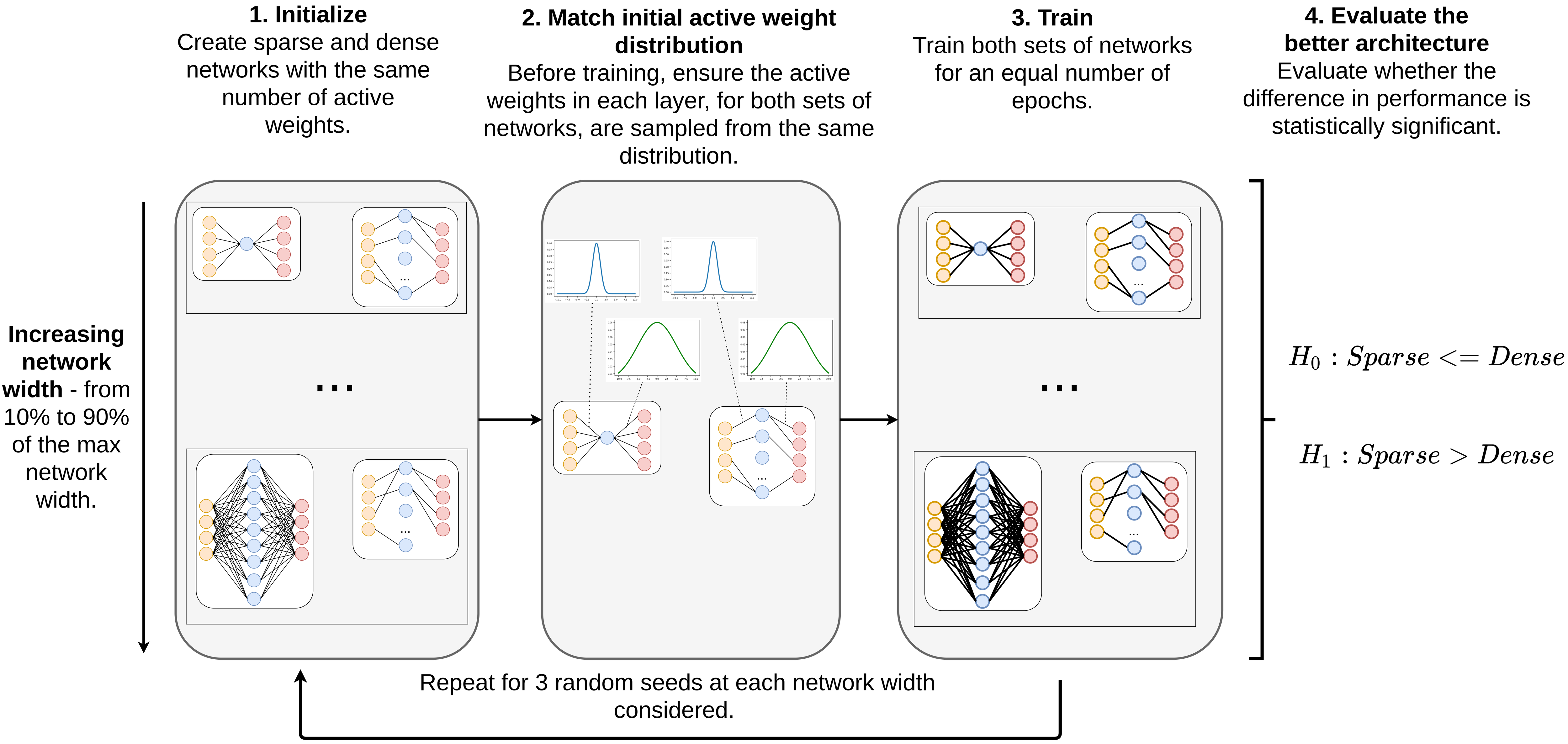
Figure 1: Same Capacity Sparse vs Dense Comparison (SC-SDC). SC-SDC is a simple framework that fairly compares sparse and dense networks. This is done by ensuring that the compared sparse and dense networks have the same number of active (nonzero) weights in each layer, and that these active weights are initially sampled from the same distribution.

To fairly compare sparse and dense networks, we propose Same Capacity Sparse vs Dense Comparison (SC-SDC), a simple framework that allows us to study sparse network optimization and identify which training configurations are not well suited for sparse networks.

SC-SDC can be summarized as follows (see Figure 1 for an overview):

1. Initialize For a chosen network depth (number of layers) $L$ and a maximum network width $N_{MW}$, we compare sparse network $S$ and dense network $D$ at various widths, while ensuring they have the same parameter count. Initially, we mask the weights ${\bm{\theta}}_{S}$ of sparse network $S$:

$${\bm{a}}_{S}^{l}={\bm{\theta}}_{S}^{l}\odot m^{l}\quad,\quad{\bm{a}}_{D}^{l}={\bm{\theta}}_{D}^{l},\quad\text{ for }\quad l=1,\ldots,L\quad,$$ (1)

where $\displaystyle{\bm{\theta}}_{S}^{l}\odot m^{l}$ denotes an element-wise product of the weights ${\bm{\theta}}_{S}$ of layer $l$ and the random binary matrix (mask) for layer $l$, $\displaystyle m^{l}$, $\displaystyle{\bm{a}}_{S}^{l}$ is the nonzero weights in layer $l$ of sparse network $S$, and $\displaystyle{\bm{a}}_{D}^{l}$ is the nonzero weights in layer $l$ of dense network $D$ (all the weights since no masking occurs).

For a fair comparison, we need to ensure the same number of nonzero weights for sparse network $S$ and dense network $D$ , across each layer $L$.

$$||{\bm{a}}_{S}^{l}||_{0}=||{\bm{a}}_{D}^{l}||_{0},\quad\text{ for }\quad l=1,\ldots,L$$ (2)

We provide more implementation details of how we achieve this in Appendix A.1.

2. Match active weight distributions Following prior work (Liu et al., 2018; Gale et al., 2019), we ensure that the nonzero weights at initialization of the sparse and dense networks are sampled from the same distribution at each layer as follows:

$${\bm{a}}_{S}^{l}\sim P^{l}\quad,\quad{\bm{a}}_{D}^{l}\sim P^{l},\quad\text{ for }\quad l=1,\ldots,L\quad,$$ (3)

where $P^{l}$ refers to the initial weight distribution at layer $l$. This ensures that both sets of active weights (sparse and dense) are initially sampled from the same distribution.

3. Train We then train the sparse and dense networks for the same number of epochs, allowing for convergence ($500$ epochs for Fashion-MNIST, $1000$ epochs for CIFAR-10 and CIFAR-100).

4. Evaluate the better architecture We gather the results across the different widths and conduct a paired, one-tail Wilcoxon signed-rank test (Wilcoxon, 1945) to evaluate the better architecture. We have a sample size of $30$ networks for each test configuration. This comprises of five different network widths $\times$ three independent training runs (different random seeds) $\times$ two architectures (sparse and dense variant).

Our null hypothesis ($H_{0}$) is that sparse networks have similar or worse test accuracy than dense networks (lower or the same median), while our alternative hypothesis ($H_{1}$) is that sparse networks have better test accuracy performance than dense networks of the same capacity (higher median). This can be formulated as:

$$H_{0}:Sparse<=Dense\quad,\quad H_{1}:Sparse>Dense$$ (4)

2.2 Measuring Gradient Flow

Gradient flow (GF) is used to study optimization dynamics and is typically approximated by taking the norm of the gradients of the network (Pascanu et al., 2013; Nocedal et al., 2002; Chen et al., 2018; Wang et al., 2020; Evci et al., 2020). Looking at gradient flow is particularly relevant in the context of sparse networks, since they are sensitive to poor gradient flow (Wang et al., 2020; Evci et al., 2020). Hence this would be a useful analysis tool for their optimization.

We consider a feedforward neural network $\displaystyle f:\mathbb{R}^{D}\rightarrow\mathbb{R}$, with function inputs $\displaystyle\mathbf{x}\in\mathbb{R}^{D}$ and network weights ${\bm{\theta}}$. The gradient norm is usually computed by concatenating all the gradients of a network into a single vector, ${\bm{g}}=\frac{\partial\mathcal{C}}{\partial{\bm{\theta}}}$ , where $C$ is our cost function. Then the vector norm is taken as follows:

$$gf_{p}=||{\bm{g}}||_{p}\quad,$$ (5)

where $p$ denotes the pth-norm and $gf_{p}$ is the gradient flow. Traditional gradient flow measures take the $L1$ or $L2$ norm of all the gradients (Chen et al., 2018; Pascanu et al., 2013; Evci et al., 2020). Unless gradients are masked before calculating the gradient flow, the standard gradient flow formulation could result in gradients of masked weights, which do not influence the forward pass, being included in the formulation. Furthermore, computing the $L1$ or $L2$ gradient norm by concatenating all the gradients into a single vector gives disproportionate influence to layers with more weights.

Effective Gradient Flow To address these shortcomings with the standard $gf_{p}$ measures, we propose a simple modification of Equation 5, which we term Effective Gradient Flow (EGF), that computes the average, masked gradient (only gradients of active weights) norm across all layers.

We calculate EGF as follows:

$${\bm{g}}=(\frac{\partial\mathcal{C}}{\partial{\bm{\theta}}^{1}}\odot m^{1},\frac{\partial\mathcal{C}}{\partial{\bm{\theta}}^{2}}\odot m^{2},\dots,\frac{\partial\mathcal{C}}{\partial{\bm{\theta}}^{L}}\odot m^{L})\quad,$$ (6)

$$EGF_{p}=\dfrac{\sum\limits_{n=1}^{L}{||{\bm{g}}_{n}||_{p}}}{L}\quad,$$ (7)

where $L$ is the number of layers. For every layer $l$, $\displaystyle\frac{\partial\mathcal{C}}{\partial\theta^{l}}\odot m^{l}$ denotes an element-wise product of the gradients of layer $l$, $\displaystyle\frac{\partial\mathcal{C}}{\partial\theta^{l}}$ , and the mask $\displaystyle m^{l}$ applied to the weights of layer $l$. For a fully dense network, $m^{l}$ is a matrix of all ones, since no gradients are masked.

EGF has the following favourable properties:

• Gradient Flow Is Evenly Distributed Across Layers EGF distributes the gradient norm across the layers equally. This prevents layers with many weights from dominating the measure, and prevents layers with vanishing gradients from being hidden in the formulation, as is the case with equation 5 (when all gradients are appended together).

• Only Gradients of Active Weights Are Used EGF ensures that for sparse networks, only gradients of active weights are used. Even though weights are masked, their gradients are not necessarily zero since the partial derivative of the weight w.r.t. the loss is influenced by other weights and activations. Therefore, even though the weight is zero, its gradient can be nonzero.

• Possibility for Application in Gradient-based Pruning Methods Tanaka et al. (2020) showed that gradient-based pruning methods like GRASP (Wang et al., 2020) and SNIP (Lee et al., 2018), disproportionately prune large layers and are susceptible to layer-collapse, which is when an algorithm prunes all the weights in a specific layer. Since EGF is evenly distributed across layers, maintaining EGF (as opposed to standard gradient norm) could be used as pruning criteria. Furthermore, current approaches measuring or approximating the change in gradient flow during pruning in sparse networks (Wang et al., 2020; Evci et al., 2020; Lubana & Dick, 2021), could benefit from this new formulation.

To evaluate EGF against other standard gradient norm measures, such as the $L1$ and $L2$ norm, we empirically compare these measures and their correlation to test loss and accuracy. We take the average of the absolute Kendall Rank correlation (Kendall, 1938), across the different experiment configurations. We follow a similiar approach to Jiang et al. (2019), but unlike their work which has focused on correlating network complexity measures to the generalization gap, we measure the correlation of gradient flow to performance (accuracy and loss). We measure gradient flow at points evenly spaced throughout training.

Our results from Table 1 show that in sparse networks, EGF consistently has a higher average absolute correlation to both test loss and accuracy. We see that EGF has similar correlation to standard gradient flow measures in dense networks. This shows that the benefits of using EGF are more apparent when used in conjunction with sparse networks, since EGF only considers the gradients of nonzero weights. Due to the comparative benefits of EGF in sparse networks, we use it for the remainder of the paper to measure the impact of interventions. We include experimental results using other gradient flow measures in Appendix B for completeness.

	Measure	Sparse		Dense
		Test Loss	Test Accuracy	Test Loss	Test Accuracy
FMNIST	$||{\bm{g}}||_{1}$	0.355	0.316	0.365	0.354
	$||{\bm{g}}||_{2}$	0.282	0.292	0.285	0.329
	$EGF_{1}$	0.419	0.373	0.365	0.354
	$EGF_{2}$	0.360	0.323	0.298	0.320
CIFAR-10	$||{\bm{g}}||_{1}$	0.440	0.327	0.380	0.251
	$||{\bm{g}}||_{2}$	0.447	0.308	0.355	0.290
	$EGF_{1}$	0.371	0.300	0.380	0.252
	$EGF_{2}$	0.451	0.332	0.363	0.287
CIFAR-100	$||{\bm{g}}||_{1}$	0.355	0.385	0.325	0.319
	$||{\bm{g}}||_{2}$	0.373	0.393	0.357	0.385
	$EGF_{1}$	0.358	0.320	0.325	0.319
	$EGF_{2}$	0.402	0.396	0.359	0.382

Table 1: The Average Correlation Between Gradient Flow Measures and Generalization Performance. We compare the average, absolute Kendall Rank correlation (Kendall, 1938) between different formulations of gradient flow and generalization (test loss and test accuracy). The subscripts ($1$ or $2$) denote the $p$-norm ($l1$ or $l2$ norm). We see that for sparse networks, our proposed measure, EGF (Equation 6), consistently has higher absolute correlation to performance compared to standard gradient flow measures ($||{\bm{g}}||_{1}$ and $||{\bm{g}}||_{2}$, Equation 5). For each dataset, we highlight the measure with the highest correlation to performance in bold.

Configuration	Variants
Optimizers	Adagrad, Adam, RMSProp, SGD and SGD with mom (0.9).
Regularization/Normalization	No Regularization (NR), Weight Decay (L2), Data Augmentation (DA), Skip Connections (SC) and BatchNorm (BN).
Number of hidden layers	1, 2 and 4.
Dense Width	308, 923, 1538, 2153 and 2768.
Activation functions	ReLU, PReLU, ELU, Swish, SReLU and Sigmoid.
Learning rate	0.001 and 0.1.
Datasets	Fashion-MNIST, CIFAR-10 and CIFAR-100.

Table 2: Network Configurations. Different network configurations for Sparse and Dense Comparisons.

3 Empirical Setting

3.1 Average EGF

To measure gradient flow, we use the Average EGF calculated at the end of 11 epochs, evenly spread throughout the training. This is done because it would be computationally costly to calculate gradient norms at the end of every epoch.

3.2 Architecture, Normalization, Regularization and Optimizer Variants

We briefly describe our key experiment variants below and also include for completeness all unique variants in Table 2.

1. Activation Functions ReLU networks (Nair & Hinton, 2010) are known to be more resilient to vanishing gradients than networks that use Sigmoid or Tanh activations, since they only result in vanishing gradients when the input is less than zero, while on active paths, due to ReLU’s linearity, the gradients flow uninhibited (Glorot et al., 2011). Although most experiments are run on ReLU networks, we also explore different activation functions, namely PReLU (He et al., 2015), ELU (Clevert et al., 2015), Swish (Ramachandran et al., 2017), SReLU (Jin et al., 2015) and Sigmoid (Neal, 1992).

2. Batch Normalization and Skip Connections We empirically explore the relative benefits of BatchNorm (Ioffe & Szegedy, 2015) and skip connections (Srivastava et al., 2015; He et al., 2016) across dense and sparse networks.

3. Regularization Techniques We evaluate various popular regularization methods: weight decay/$L2$ regularization ($\lambda$ = 0.0001) (Krogh & Hertz, 1992; Hanson & Pratt, 1989) and data augmentation (random crops and random horizontal flipping (Krizhevsky et al., 2012)).

4. Optimization Techniques We benchmark the impact of the most widely used optimizers such as minibatch stochastic gradient descent (SGD) (Robbins & Monro, 1951), minibatch stochastic gradient descent with momentum (momentum term - $0.9$) (Sutskever et al., 2013; Polyak, 1964), Adam (Kingma & Ba, 2014), Adagrad (Duchi et al., 2011) and RMSProp (Hinton et al., 2012).

3.3 SC-SDC MLP Setting

We firstly use the SC-SDC empirical setting (Section 2.1) to evaluate which choices of optimizer, regularization and architecture choices result in a statistically significant performance difference between sparse and dense networks. We train $600$ MLPs for 500 epochs on Fashion-MNIST (FMNIST) (Xiao et al., 2017) and over $10\,000$ MLPs for 1000 epochs on CIFAR-10 and CIFAR-100 (Krizhevsky et al., 2009). We compare sparse and dense networks across various widths, depths, learning rates, regularization and optimization methods as shown in Table 2.

Dense Width Following from SC-SDC, these networks are compared at various network widths, specifically a width of 308, 923, 1538, 2153, 2768 (10%, 30%, 50%, 70% and 90% of our maximum width $N_{MW}$(3076) when using CIFAR datasets) as shown in Table 2. We use the term dense width to refer to the width of a network if that network was dense. For example, when comparing sparse and dense networks at a Dense Width of 308, this means the dense network has a width of 308, while the sparse network has a width of $N_{MW}$ (3076), but has the same number of active connections as its dense counterpart. We provide more details on Dense Width and other components of the SC-SDC implementation in Appendix A.1.

3.4 Extended CNN Setting

We also extend our experiments to CNNs and train $200$ Wide ResNet-50 (WRN) models, specifically the WRN-28-10 variant (Zagoruyko & Komodakis, 2016) for $200$ epochs on CIFAR-100. We use the same network training parameters used in the original paper (an initial learning rate of $0.1$, dropped by $0.2$ at epochs 60,120 and 160, weight decay $\lambda$ set to $0.0005$ and a momentum term of $0.9$).

4 Results and Discussion

We present our results studying sparse network optimization in MLPs, using SC-SDC and EGF. Furthermore, we extend our results outside of SC-SDC, from MLPs to CNNs and from Random Pruning to Magnitude Pruning.

For brevity, we use a shorthand notation for our different regularization/normalization methods — no regularization (NR), weight decay (L2), data augmentation (DA), skip connections (SC) and BatchNorm (BN). When multiple of these methods are combined, we chain their abbreviations such as DA_BN, which represents data augmentation and BatchNorm combined. Furthermore, for our discussion, we make a distinction between optimization methods that use exponential weighted moving averages, also known as leaky averaging, for estimates of the variance of their gradients (EWMA optimizers) - specifically Adam and RMSProp, and methods which do not - Adagrad, SGD and SGD with momentum. We provide details on this distinction in Appendix C.

4.1 Comparison of Dense and Sparse Interventions Using SC-SDC

In this section, we use the results from SC-SDC to identify which optimization choices are currently well suited for sparse networks and which are not. Most of the results discussed are achieved using four hidden layers on CIFAR-100, while we provide the full set of results for Fashion-MNIST, CIFAR-10 and CIFAR-100 in Appendix E.

4.1.1 Batch Normalization plays a disproportionate role in stabilizing Sparse Networks

BatchNorm ensures that the distribution of the nonlinearity inputs remains stable as the network trains, which was hypothesized to help stabilize gradient propagation (gradients do not explode or vanish) (Ioffe & Szegedy, 2015).

In Non-EWMA Optimizers, BatchNorm Favours Sparse Networks From Table 3(c) and 3(c), we see that in non-EWMA optimizers (Adagrad, SGD and SGD with momentum), BatchNorm is statistically more significant for sparse network performance than it is for dense networks. Without BatchNorm (configurations NR, DA, L2 and SC), we see that sparse networks do not outperform their dense counterparts in test accuracy. With the addition of BatchNorm, across high and low learning rates and at most configurations (except in some cases where $L2$ is used), there is strong evidence that sparse networks outperform dense networks.

In EWMA Optimizers, BatchNorm Brings Sparse and Dense Networks Closer in Performance When Adam or RMSProp are used as optimization algorithms, we see that sparse networks outperform dense networks without BatchNorm (NR from Table 3(c) and 3(c)). When BatchNorm is added to these methods (BN), we see that sparse networks lose their advantage and they perform similarly or slightly better than their dense counterparts in test accuracy and gradient flow, as can be seen from Figure 2.

At Shallow Depths, BatchNorm is More Critical to Performance than Skip Connections Figures 2(a) and 2(c) show that BatchNorm (BN) is more critical in terms of test accuracy than skip connections (SC). Furthermore, we see that BatchNorm (BN) performs similarly, in terms of test accuracy, to skip connections and BatchNorm combined (SC_BN). This suggests that skip connections do not provide a performance benefit when applied with BatchNorm. We believe this is due to the shallow depth of these networks (four hidden layers), as skip connections have proved to be critical for deeper networks, even with BatchNorm (Balduzzi et al., 2017; Yang et al., 2019; Labatie, 2019).

BatchNorm Stabilizes Gradient Flow Across all optimizers and learning rates, we see that when BatchNorm is used, it results in a lower, more stable EGF (Figures 2(b) and 2(d)), compared to the original network without BatchNorm (comparing NR to BN, L2 to L2_BN, DA to DA_BN and SC to SC_BN). This further emphasizes the importance of BatchNorm in stabilizing gradient flow.

(a) Different Regularization Methods - Low learning rate (0.001)

	NR	DA	L2	SC	BN	DA_BN	L2_BN	SC_BN
Adagrad	1.000	1.000	0.998	0.239	0.006	0.002	0.001	0.003
Adam	0.000	0.055	0.198	0.003	0.079	0.051	0.254	0.166
RMSProp	0.001	0.000	0.300	0.166	0.117	0.021	0.914	0.541
SGD	1.000	1.000	1.000	0.248	0.000	0.000	0.001	0.003
Mom (0.9)	1.000	1.000	1.000	0.999	0.001	0.000	0.007	0.008

(b) Different Regularization Methods - High learning rate (0.1)

	BN	DA_BN	L2_BN	SC_BN	DA_SC_BN	DA_L2_SC_BN
Adagrad	0.000	0.002	0.963	0.002	0.023	0.014
Adam	0.070	0.002	0.043	0.004	0.191	0.377
RMSProp	0.002	0.027	0.008	0.562	0.894	0.002
SGD	0.001	0.000	0.048	0.005	0.001	0.013
Mom (0.9)	0.001	0.002	0.488	0.003	0.005	0.212

(c) Different Activation Functions - High learning rate (0.1)

	ReLU	Swish	PReLU	SReLU	Sigmoid	ELU
Adagrad	0.023	0.005	0.050	0.182	0.568	0.003
Adam	0.191	0.182	0.039	0.062	0.005	0.000
RMSProp	0.894	0.167	0.002	0.012	0.997	0.153
SGD	0.013	0.027	0.005	0.078	0.030	0.056
Mom (0.9)	0.212	0.013	0.001	0.078	0.001	0.973

Table 3: Wilcoxon Signed Rank Test Results for MLPs with Four Hidden Layers, Trained on CIFAR-100. We show the results using different optimization and regularization methods, across various sparsity levels as mentioned in Section 3.3. We use a $p$-value of 0.05, with the bold values indicating where we can be statistically confident that sparse networks perform better than dense (reject $H_{0}$ from 4). We also use a continuous colour scale to make the results more interpretable. This scale ranges from green (0 - likely that sparse networks perform better than dense) to yellow (0.5 - 50% chance that sparse networks perform better than dense) to red (1 - highly likely that sparse networks do not outperform dense - cannot reject $H_{0}$ from 4). The performance results for all these networks are present in Appendix E.

Colour Scale based on p-values : 0 .5 1 S $>$ D S $\leq$ D

NR - No Regularization, BN - Batchnorm, SC - Skip Connections, DA - Data Augmentation, L2- weight decay, D - Dense Networks and S - Sparse Networks.

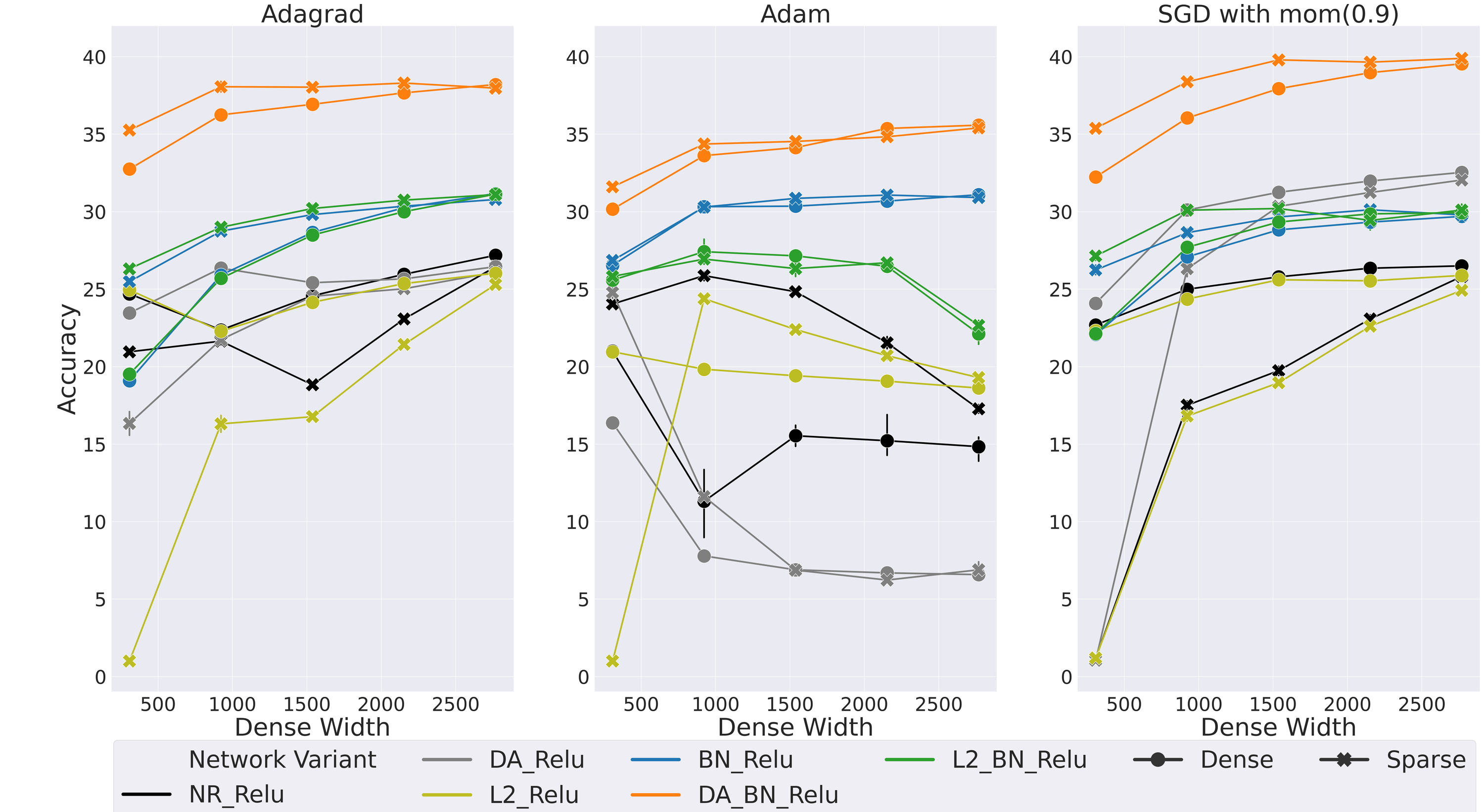
(a) Test Accuracy - Low learning rate (0.001)

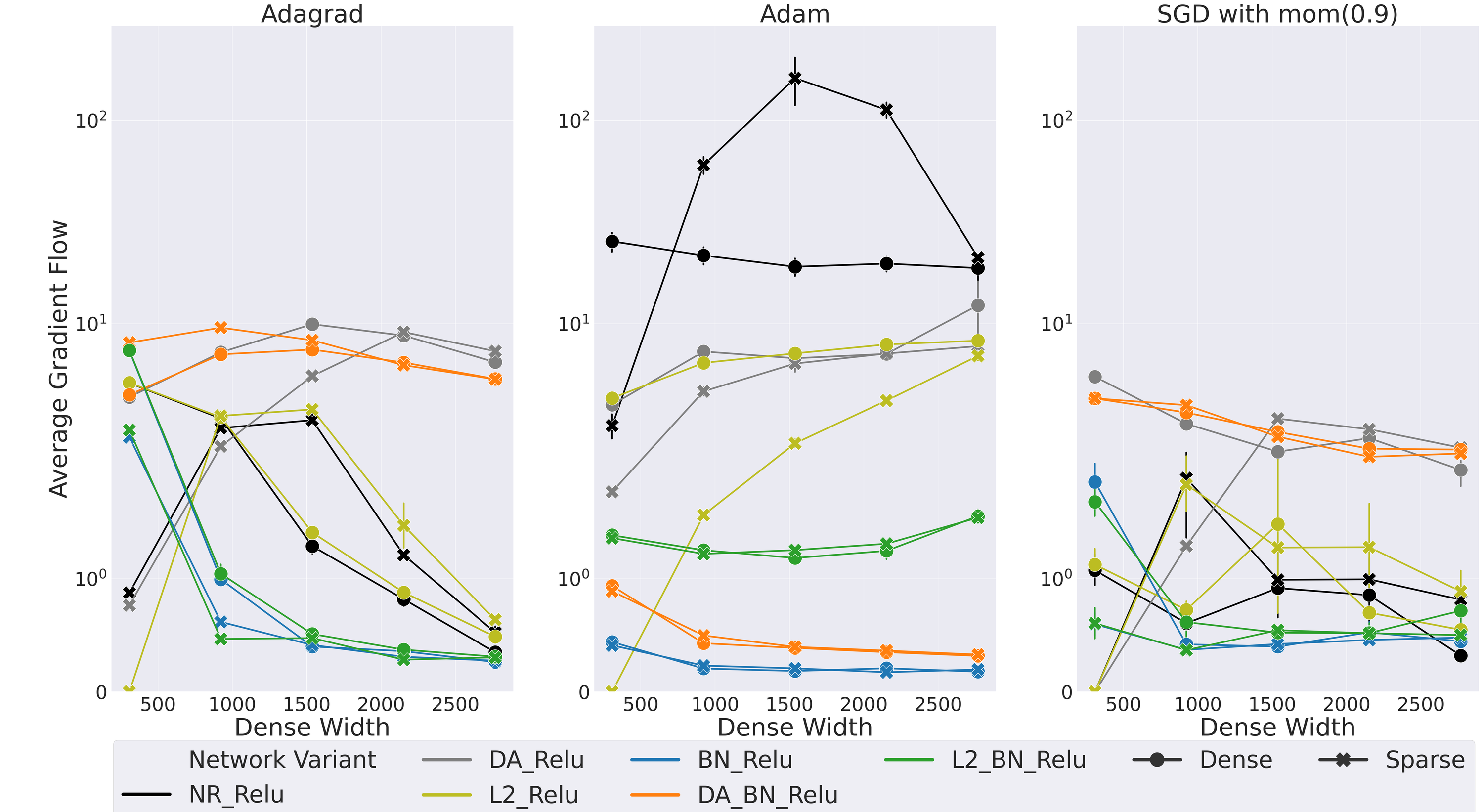
(b) Gradient Flow - Low learning rate (0.001)

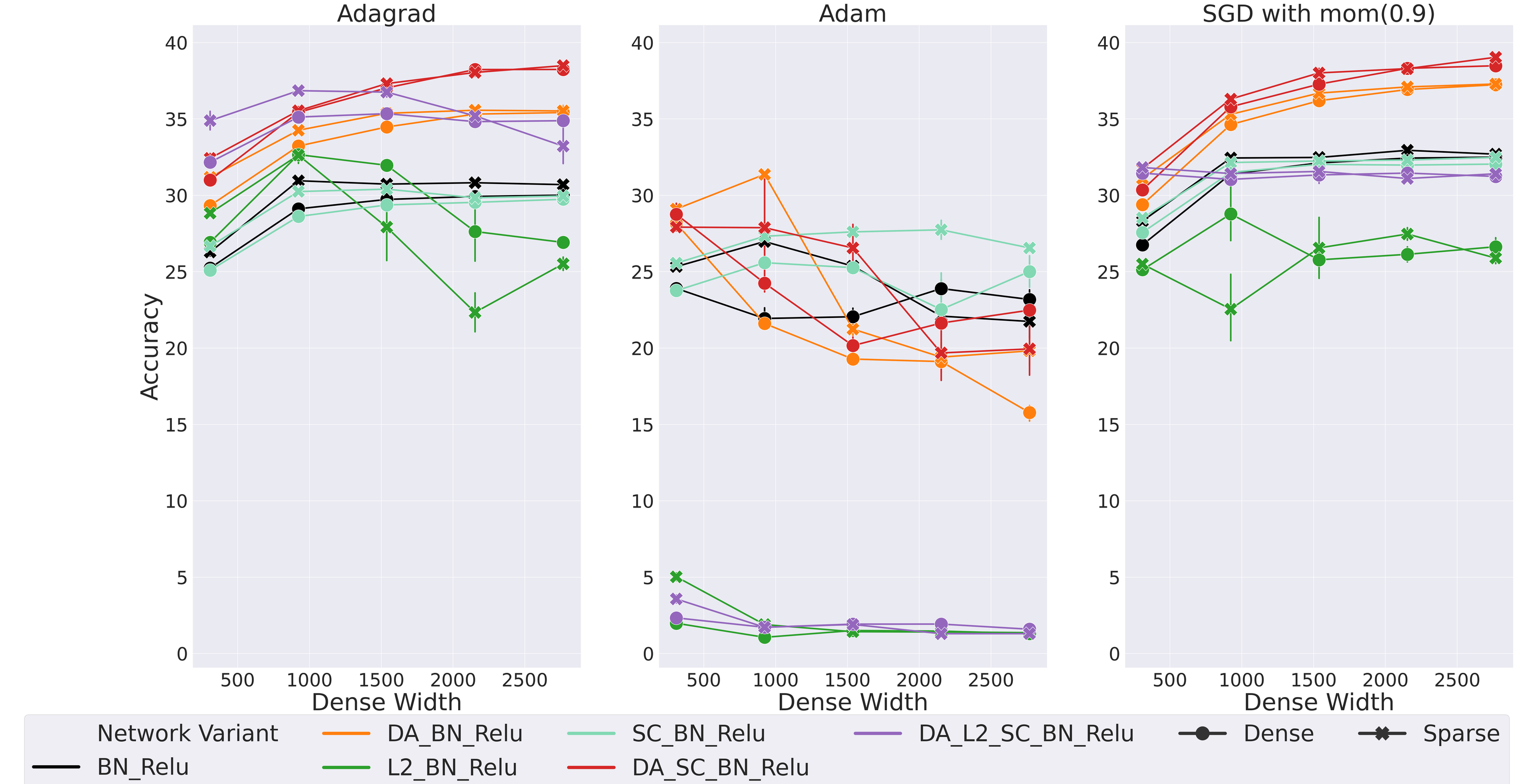
(c) Test Accuracy - High learning rate (0.1)

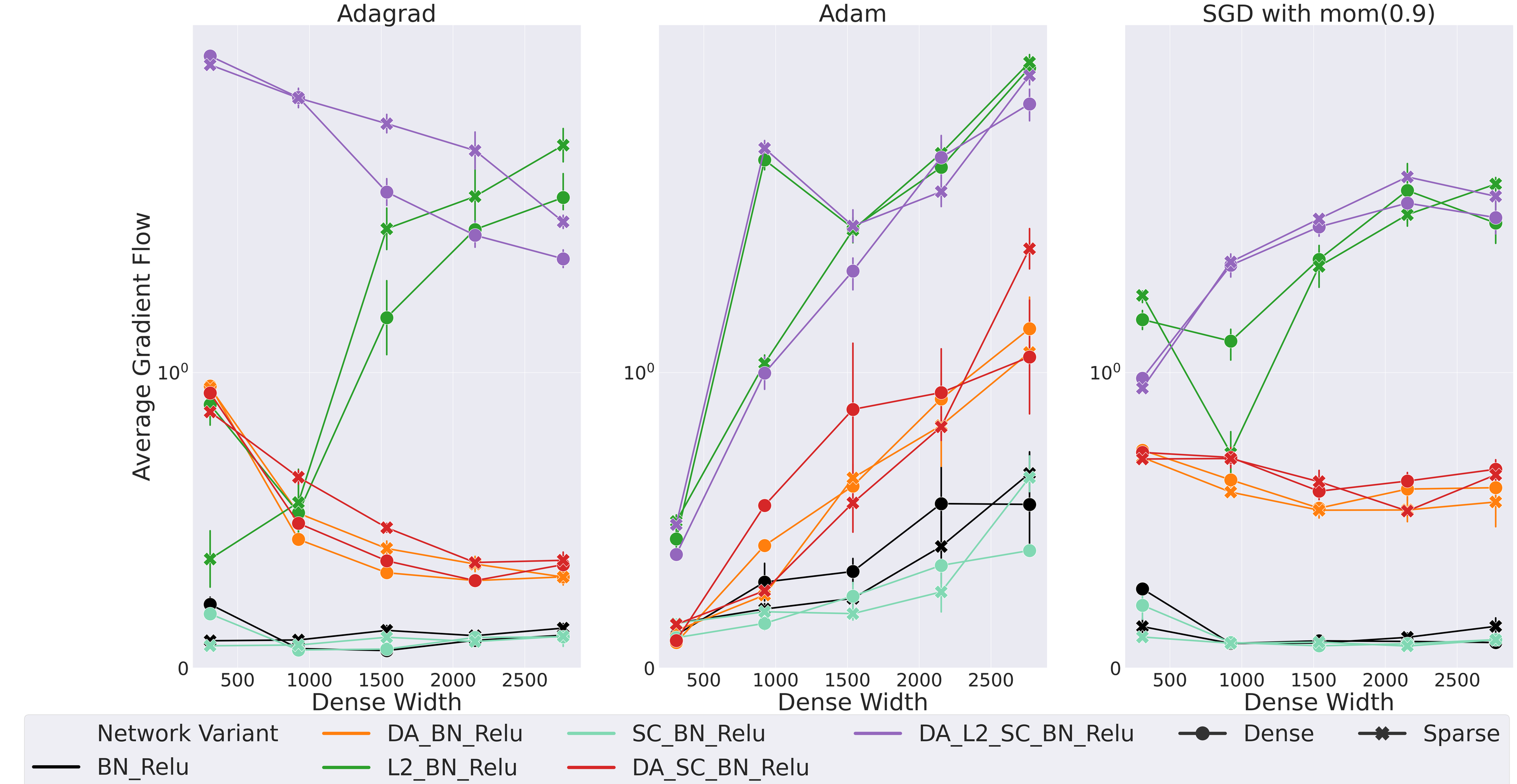
(d) Gradient Flow - High learning rate (0.1)

NR - No Regularization, BN - Batchnorm, SC - Skip Connections, DA - Data Augmentation and L2- weight decay.

Figure 2: Test Accuracy and Gradient Flow in Sparse and Dense MLPs. We study the effect of different regularization and optimization methods on test accuracy and average gradient flow, across different learning rates. We see that for Adam, a higher gradient flow tends to correlate to poor performance. The results for all optimizers can be found in Figures 19 and 21.

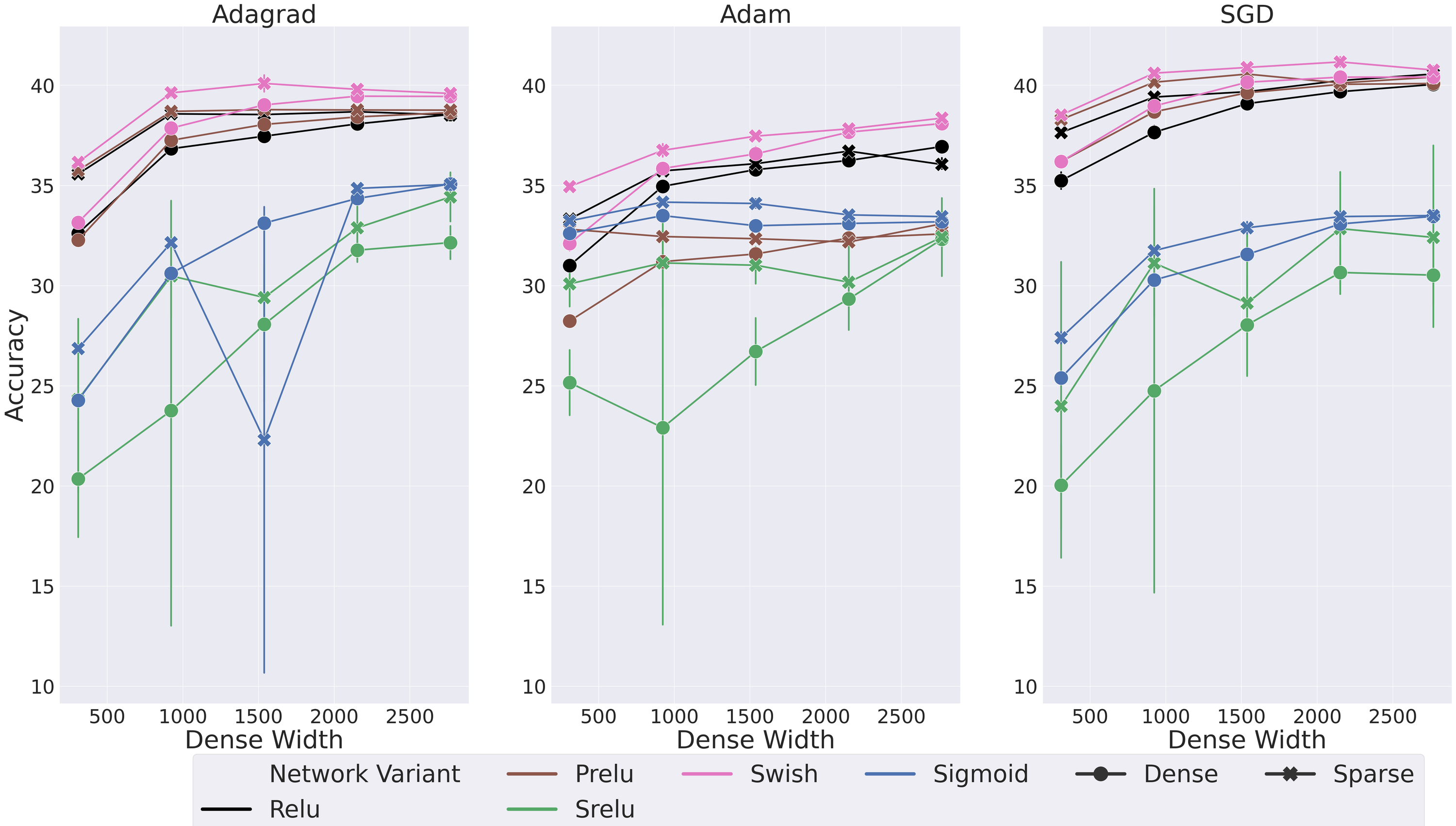
(a) Test Accuracy

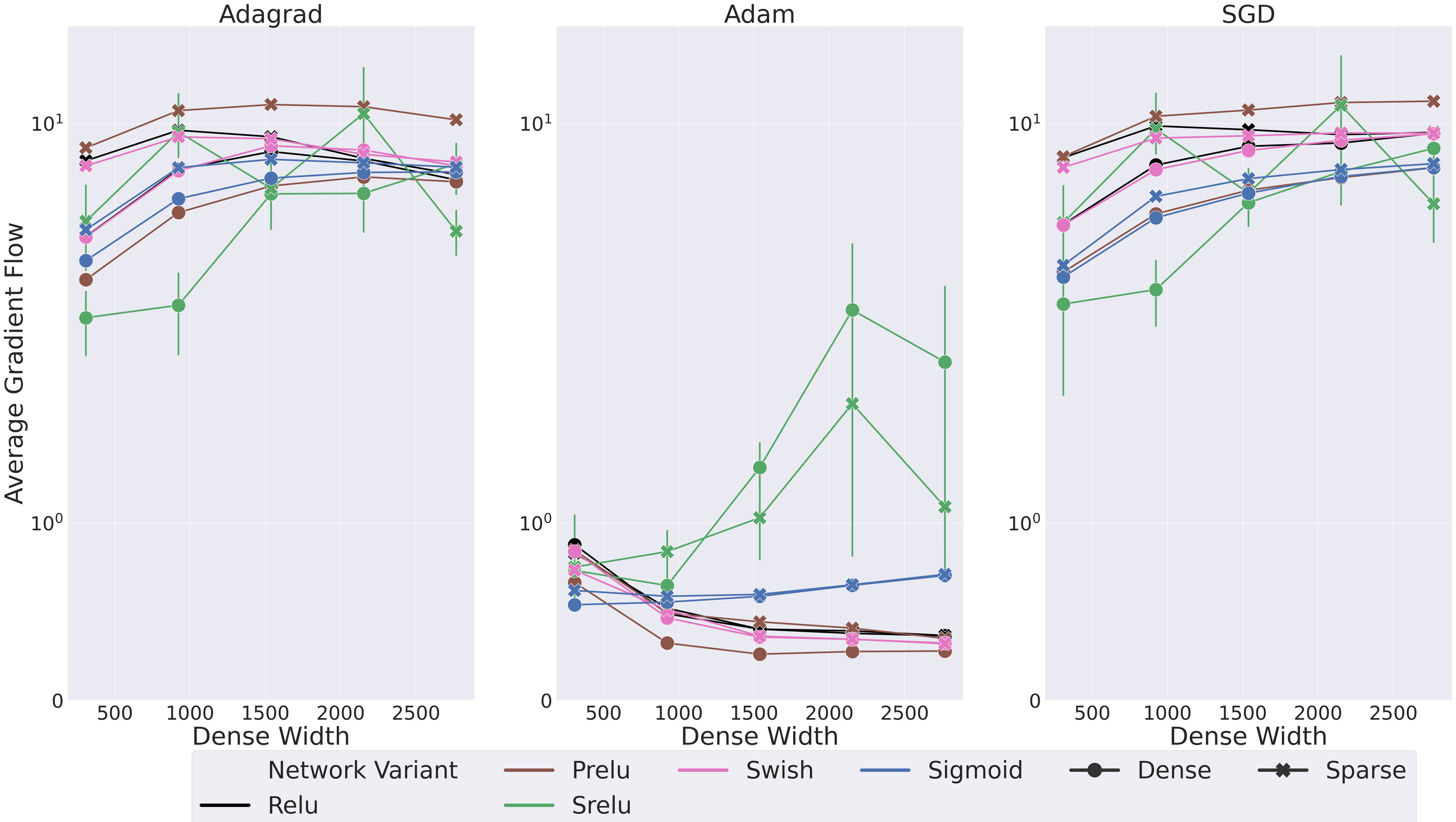
(b) Gradient Flow

Figure 3: Effect of Activation Functions on Accuracy and Gradient Flow on CIFAR-100, With a Low Learning Rate (0.001). We see that Swish is the most promising activation function across most optimizers. The results across all optimizers and learning rates are shown in Figure 20 and 22.

4.1.2 EWMA optimizers are sensitive to high gradient flow

In EWMA Optimizers, $L2$ Regularization can hurt Network Performance For networks without BatchNorm and with $L2$ regularization (configuration $L2$), we can see from Figure 2(a) that when using adaptive methods (Adagrad, Adam and RMSProp), $L2$ regularization mainly hurts sparse network performance. This occurs particularly at high sparsity levels (a dense width of less than 2153). Conversely, equivalent capacity and configured dense networks achieve a performance improvement with $L2$ regularization, compared to their base configuration (comparing NR to L2).

For networks with BatchNorm, trained with EWMA optimizers, $L2$ regularization adversely affects both sparse and dense network performance. From Figures 2(c) and 2(d), we see that the addition of $L2$ (configurations L2_BN and DA_L2_SC_BN) drastically decreases the accuracy of these networks. When we analyse their EGF, from Figure 2(d), we see that the addition of $L2$ consistently across all optimizers results in distinctively larger EGF values. This hints at EWMA optimizers being more sensitive to larger gradient norms than other optimizers.

The poor performance of adaptive methods with $L2$ regularization (specifically EWMA optimizers) agrees with Loshchilov & Hutter (2017). They proposed a different formulation of weight decay for Adam, named AdamW, since the current $L2$ regularization formulation for adaptive methods could lead to weights with large gradients being regularized less. We experimentally verified this in Figure 23, showing that the AdamW’s weight decay formulation has a lower EGF than the standard $L2$ formulation used in Adam, and this correlates to better network performance in AdamW.

Data Augmentation Favours Non-EWMA Optimizers When networks are trained with data augmentation and without BatchNorm (configuration DA), we see poor test accuracy for EWMA optimizers, across sparse and dense networks (Figure 2(a)). With the addition of BatchNorm (configuration BN_DA), when using a low learning rate, we see that data augmentation benefits all optimizers (Figure 2(a)). This behaviour differs when using a high learning rate (Figure 2(c)), where data augmentation results in a higher gradient flow in all optimizers (comparing BN to DA_BN). This then results in lower performance in EWMA optimizers, further emphasizing the sensitivity of these optimizers to higher gradient flow.

For non-EWMA optimizers, data augmentation consistently increases performance, even with a higher learning rate and higher EGF, which suggests data augmentation is better suited for these methods.

EWMA Optimizers Struggle with High Gradient Flow If we take a closer look at the gradient flow, through the average EGF (Figures 2(b) and 2(d)), we see that for EWMA optimizers the worst performing variants (L2, NR, DA, L2_BN and DA_L2_SC_BN) consistently have a relatively high EGF, while the best performing interventions (BN, BN_SC and DA_BN_SC) have a lower EGF. This is also true of different activation functions, where the worst performing activation function when using Adam, SReLU, also has the highest EGF (Figure 3).

In non-EWMA optimizers, a higher gradient flow does not consistently lead to poor performance. This hints that the higher effective learning rates of EWMA optimizers can be problematic during training, primarily when used in conjunction with methods that result in high EGF. The sensitivity of networks trained with EWMA optimizers, particularly sparse networks, to $L2$ and data augmentation suggests that, in their current formulation, these methods are not adequate for sparse networks.

4.1.3 The potential of non-sparse activation functions - Swish and PReLU

We also explore the impact of different activation functions - specifically PReLU (He et al., 2015), ELU (Clevert et al., 2015), Swish (Ramachandran et al., 2017), SReLU (Jin et al., 2015) and Sigmoid (Neal, 1992) - on network performance. The best regularization configuration for each optimizer was chosen.

From Table 3(c) and 6(b), we see that Swish and PReLU consistently favour sparse networks across most optimizers in a statistically significant manner. From the performance results shown in Figures 3(a), 20 and 22, we see that Swish and PReLU are the most promising activation functions, with Swish being the best performing activation function in adaptive methods, and PReLU achieving promising results for networks trained with SGD.

In Appendix D, we plot the different activation functions (Figure 14(a)) and their gradients (Figure 14(b)). We see that although most activation functions, apart from ReLU, are non-sparse (do not have zero gradients), Swish is the only activation function that allows for the flow of negative gradients due to its non-monotonicity. This leads to Swish having a lower, more stable gradient flow (Figures 3(b), 20 and 22), which could explain some of its success, particularly for EWMA optimizers. We continue to see a consistent trend in EWMA methods that higher EGF values, for example in SReLU, correspond to poor performance, while promising methods, such as Swish, result in a lower EGF.

We also see that the behaviours mentioned in this section are also present in CIFAR-10 and FMNIST (Table 4 and 5, Figures 15 and 19).

4.2 Generalization of results across architecture types - Wide ResNet-50

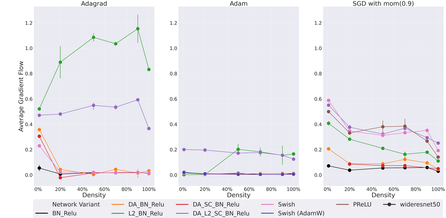
Figure 24: Wide ResNet-50 Gradient Flow on CIFAR-100. We illustrate the gradient flow of Wide ResNet-50 on CIFAR-100, with the density ranging from 1% to 100%. The accuracy results can be found in Figure 4.

We move on from SC-SDC and extend our results to more complicated, convolutional architectures. We train Wide ResNet-50 (the WRN-28-10 variant) (Zagoruyko & Komodakis, 2016) on CIFAR-100. We note from Figure 4 that most of our results from SC-SDC also hold on Wide ResNet-50, specifically that $L2$ regularization (even with BatchNorm) hurts performance for adaptive methods (Adagrad and Adam) and also results in higher EGF values (Figure 24). Furthermore, we see that Swish is a promising activation function for adaptive methods and leads to lower EGF (Figure 24). Finally, we see that the combination of Swish and AdamW (configuration Swish (AdamW)) achieve good performance for Adam, showing that the AdamW (weight decay) results from SC-SDC are also consistent in Wide ResNet-50. These results show that the SC-SDC results are not constrained to small scale experiments and that they can be used to learn about the dynamics of larger, more complicated networks.

4.3 Generalization of results from Random Pruning to Magnitude Pruning

We briefly validate if some of our results achieved through random pruning, extend to magnitude pruning (Zhu & Gupta, 2017; Han et al., 2015). For a comparable experimental setting to section 4.2, we train dense Wide ResNet-50 for 100 epochs (50% of the training time) and use magnitude pruning to achieve the desired sparsity, and then fine-tune for the remaining 100 epochs. From Figures 5(a) and 5(b), we see that although it appears magnitude pruned networks are more susceptible to vanishing gradients, these networks behave similarly to randomly pruned networks. In these networks, $L2$ regularization leads to high EGF values (L2_BN and DA_L2_SC_BN), which correlates to poor performance for EWMA optimizers (Adam). This provides evidence that some of the results achieved on random, sparse networks also extend to magnitude pruned networks.

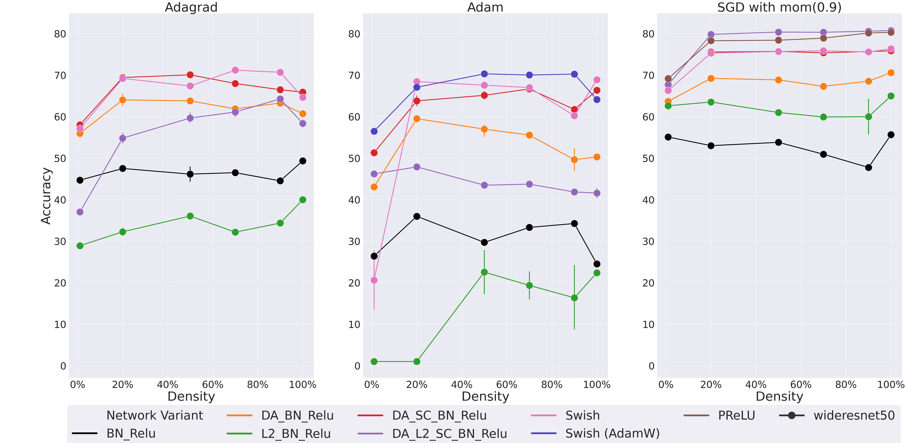
Figure 4: Wide ResNet-50 Test Accuracy on CIFAR-100. We see that the results achieved on MLPs, using SC-SDC, are also consistent in CNNs. The densities range from 1% to 100% (fully dense) and the gradient flow results can be found in Figure 24.

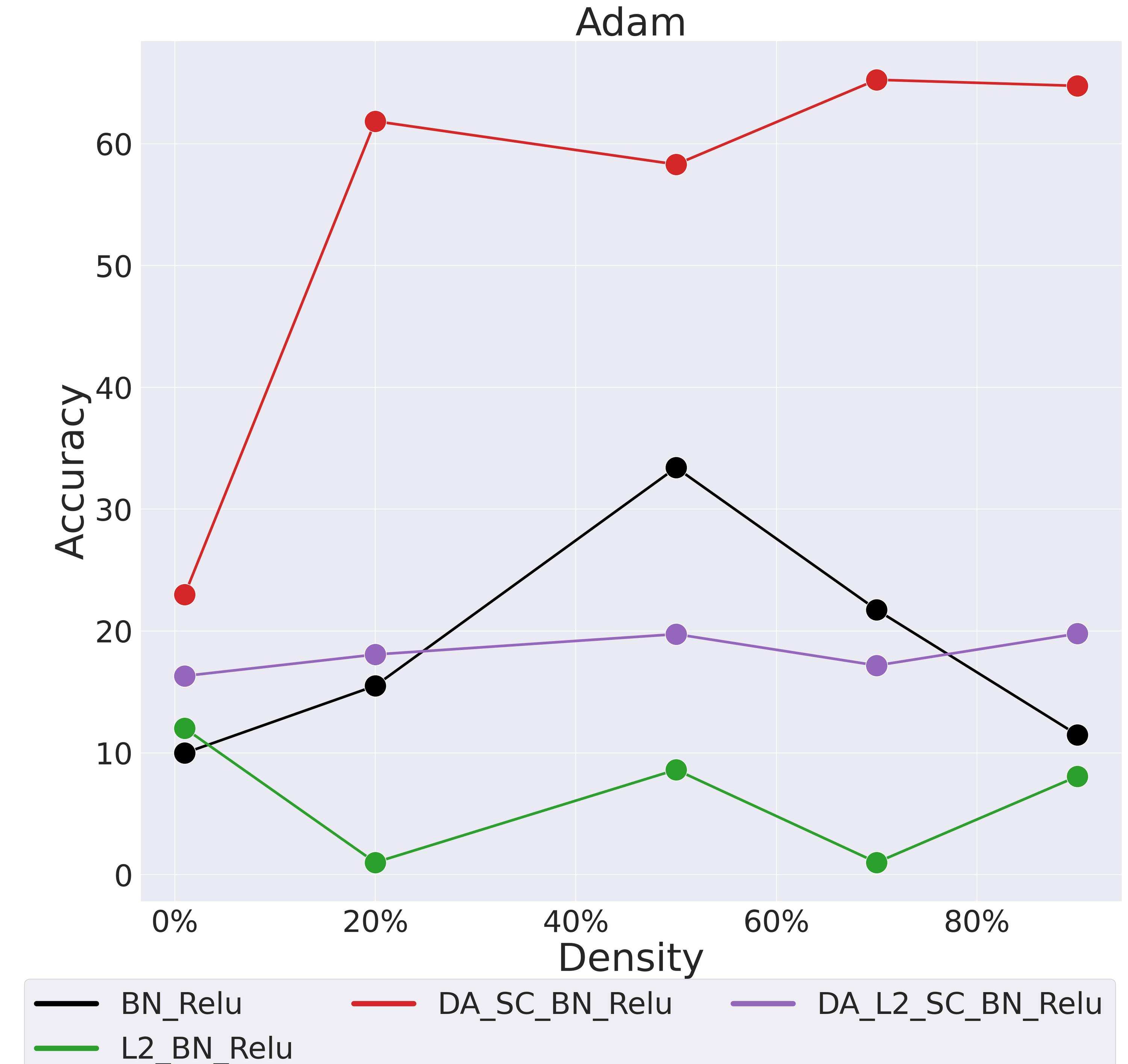
(a) Test Accuracy - Magnitude Pruning

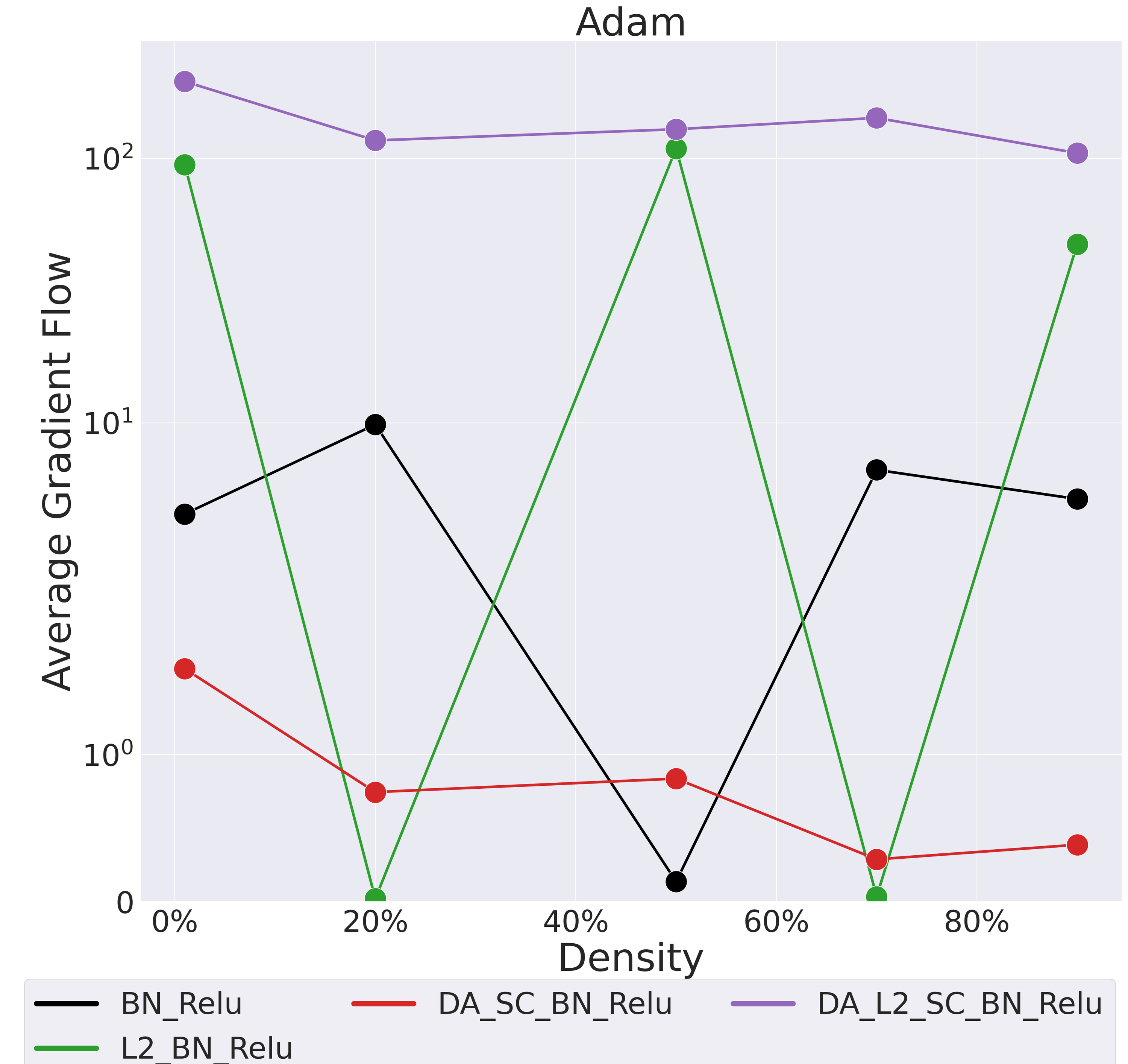
(b) Gradient Flow - Magnitude Pruning

Figure 5: Accuracy and Gradient Flow for Magnitude Pruning. We see that similarly to randomly pruned networks, magnitude pruned networks trained with Adam and $L2$ lead to high EGF and poor performance.

5 Related work

Pruning at Initialization Methods that prune at initialization aim to start sparse, instead of first pre-training an overparameterized network and then pruning. These methods use certain criteria to estimate which weights should remain active at initialization. This criteria includes using the connection sensitivity (Lee et al., 2018), gradient flow (via the Hessian vector product) (Wang et al., 2020) and conservation of synaptic saliency (Tanaka et al., 2020).

Pruning during Training Another branch of pruning is Dynamic Sparse Training, which uses information gathered during the training process, to dynamically update the sparsity pattern of these sparse networks (Mostafa & Wang, 2019; Bellec et al., 2017; Mocanu et al., 2018; Dettmers & Zettlemoyer, 2019; Evci et al., 2019). While our work is motivated by the same goal of improving the performance of sparse networks and allowing them to converge to the same performance as dense networks, we instead focus on the impact of optimization and regularization choices on sparse networks.

Sparse Network Optimization as Pruning Criteria Optimization in sparse networks has often been neglected in favour of studying network initialization. However, there has been work that has looked at sparse network optimization from different perspectives, mainly as a guide for pruning criteria. This includes using gradient information (Mozer & Smolensky, 1989; LeCun et al., 1989; Hassibi et al., 1993b; Karnin, 1990), approximates of gradient flow (Wang et al., 2020; Dettmers & Zettlemoyer, 2019; Evci et al., 2020), and Neural Tangent Kernel (NTK) (Liu & Zenke, 2020) to guide the introduction of sparsity.

Sparse Network Optimization to study Network Dynamics Apart from being used as pruning criteria, optimization information has been used to investigate aspects of sparse networks, such as their loss landscape (Evci et al., 2019), how they are impacted by SGD noise (Frankle et al., 2019a), the effect of different activation functions (Dubowski, 2020) and their weight initialization (Lee et al., 2019). Our work differs from these approaches as we consider more aspects of the optimization and regularization process in a controlled experimental setting (SC-SDC), while using EGF to reason about some of the results.

6 Conclusions and Future Work

In this work, we take a more comprehensive view of sparse optimization strategies and introduce appropriate tooling to measure the impact of architecture and optimization choices on sparse networks (EGF, SC-SDC).

Our results show that BatchNorm is critical to training sparse networks, more so than for dense networks, as it helps stabilize gradient flow. Furthermore, we show that EWMA optimizers (Adam (Kingma & Ba, 2014) and RMSProp (Hinton et al., 2012)) are sensitive to high gradient flow (EGF). This results in these optimizers, at times, performing poorly when used with $L2$ regularization or data augmentation. We also show the potential of non-sparse activation functions for sparse networks such as Swish (Ramachandran et al., 2017) and PReLU (He et al., 2015), with Swish’s non-monotonic formulation allowing for better gradient flow. Finally, we show that our results extend to more complicated models, like Wide ResNet-50 (Zagoruyko & Komodakis, 2016) and popular pruning methods, such as magnitude pruning (Zhu & Gupta, 2017; Han et al., 2015).

We trust that this work emphasizes that initialization is simply one piece of the sparse network puzzle and that a broader view of sparse network training is necessary for the benefits of sparsity to be fully realized. Needless to say, this research is simply the start at investigating sparse network optimization and does not cover all questions related to it. Future directions could include using EGF and SC-SDC to study other regularization methods, such as Dropout (Srivastava et al., 2014) or $L1$ regularization (Tibshirani, 1996), or other normalization methods, such as Layer Normalization (Ba et al., 2016). Furthermore, these tools could inspire novel pruning, regularization, or optimization techniques, that are grounded in stabilizing the gradient flow in sparse networks.

Appendix A SC-SDC

In this section, we provide more information about SC-SDC and its benefits.

A.1 SC-SDC implementation details

Wilcoxon Signed Rank Test SC-SDC uses the Wilcoxon Signed Rank Test as the statistical test to compare sparse and dense networks. This test is a non-parametric statistical test that compares dependent or paired samples, without assuming the differences between the paired experiments are normally distributed (McDonald, 2009; Demšar, 2006).

Random Sparsity Our work focuses on the training dynamics of random, sparse networks. We achieve random sparsity, by generating a random mask for each layer and then multiply the weights by this mask during each forward pass. The sparsity is distributed evenly across the network. For example, a 20% sparse MLP has 20% of the weights remaining in each layer.

Dense Width A critical component to how we specify our experiments is a term we define as dense width. In order to fairly compare sparse and dense networks, we need them to have the same number of active connections at each depth. In the case of sparse networks, this means ensuring they have the same number of active connections as the dense networks, while remaining sparse. Dense width refers to the width of a network if that network was dense. This process of comparing sparse and dense networks at different dense widths is illustrated in Figure 7.

Fair Comparison of Sparse and Dense Networks As can be seen from Figure 7, SC-SDC ensures the exact same active parameter count, but the sparse networks will be connected to more neurons. It is possible that the increased number of activations being used can lead to sparse networks having higher representational power. However, most work on expressivity of neural networks looks at this from a depth perspective and proves certain depths of networks are universal approximators (Eldan & Shamir, 2016; Hornik et al., 1989; Funahashi, 1989). To this end, we ensure these networks have the same depth, but we believe going forward an interesting direction would be ensuring they have a similar amount of active neurons.

SC-SDC Comparison Details For completeness, we provide more details of how we ensure sparse and dense networks are of the same capacity.

Following from Equation 2, to ensure the same number of weights in sparse and dense networks, we can ensure they have the same number of active weights at each layer as follows:

$$||{\bm{a}}_{S}^{l}||_{0}=||{\bm{a}}_{D}^{l}||_{0},\quad\text{ for }\quad l=1,\ldots,L\qquad,$$ (8)

where $\displaystyle{\bm{a}}_{S}^{l}$ is the nonzero weights in layer $l$ of sparse network $S$ and $\displaystyle{\bm{a}}_{D}^{l}$ is the nonzero weights in layer $l$ of dense network $D$ (all the weights since no masking occurs).

This is achieved by masking each of the weight layers of sparse network $S$:

$${\bm{a}}_{S}^{l}={\bm{\theta}}_{S}^{l}\odot m^{l}\quad\text{ for }\quad l=1,\ldots,L\qquad,$$ (9)

where $m^{l}$ is a random binary matrix (mask) for layer $l$, s.t. $||m^{l}||_{0}=||{\bm{a}}_{D}^{l}||_{0}$, where $||{\bm{a}}_{D}^{l}||_{0}$ is the number of active (nonzero) weights in the dense network and is determined by the chosen comparison width.

For SC-SDC, we need a maximum network width $N_{MW}$ and comparison width $N_{W}$. We choose a max network width $N_{MW}$ of $n+4$, where $n$ is the input dimension of the network. In the case of CIFAR, $n=3072$ and so our maximum width $N_{MW}=3076$. The choice of $n+4$ follows from Lu et al. (2017), where the authors prove a universal approximation theorem for width-bounded ReLU networks, with width bounded to $n+4$. Our comparison width, $N_{W}$, is equivalent to dense widths we vary in our experiments - 308, 923, 1538, 2153, 2768 (10%, 30%, 50%, 70% and 90% of our maximum width $N_{MW}$(3076) when using CIFAR datasets).

The dimensions of each of layers of the different networks, $S$ (sparse) and $D$ (dense), are as follows:

1. First Layer:

   $${\bm{\theta}}_{D}^{1}\in\mathbb{R}^{I\times N_{W}}\quad,\quad\displaystyle{\bm{\theta}}_{S}^{1}\in\mathbb{R}^{I\times N_{MW}}\quad,\quad m^{1}\in\{0,1\}^{I\times N_{MW}}\quad\quad\\$$ (10)

2. Intermediate Layers:

   $${\bm{\theta}}_{S}^{1}\in\mathbb{R}^{N_{W}\times N_{W}}\quad,\quad\displaystyle{\bm{\theta}}_{S}^{1}\in\mathbb{R}^{N_{MW}\times N_{MW}}\quad,\quad m^{\{2,\dots,L-1\}}\in\{0,1\}^{N_{MW}\times N_{MW}}$$ (11)

3. Final Layer:

   $${\bm{\theta}}_{S}^{L}\in\mathbb{R}^{N_{W}\times O}\quad,\quad\displaystyle{\bm{\theta}}_{S}^{L}\in\mathbb{R}^{N_{MW}\times O}\quad,\quad m^{L}\in\{0,1\}^{N_{MW}\times O}$$ (12)

, where $N_{MW}$ is maximum width of the sparse layer, $N_{W}$ is the comparison width, $I$ is the input dimension, $O$ is output dimension, $L$ is the number of layers in the network, $\displaystyle{\bm{\theta}}_{S}^{l}$ is the weights in layer $l$ of sparse network $S$ and $\displaystyle{\bm{\theta}}_{D}^{l}$ is the weights in layer $l$ of dense network $D$.

This process would be the same for convolutional layers, but there would be a third dimension to handle the different channels. In Figure 6, we provide an illustrative example showing how to ensure sparse and dense networks are compared fairly.

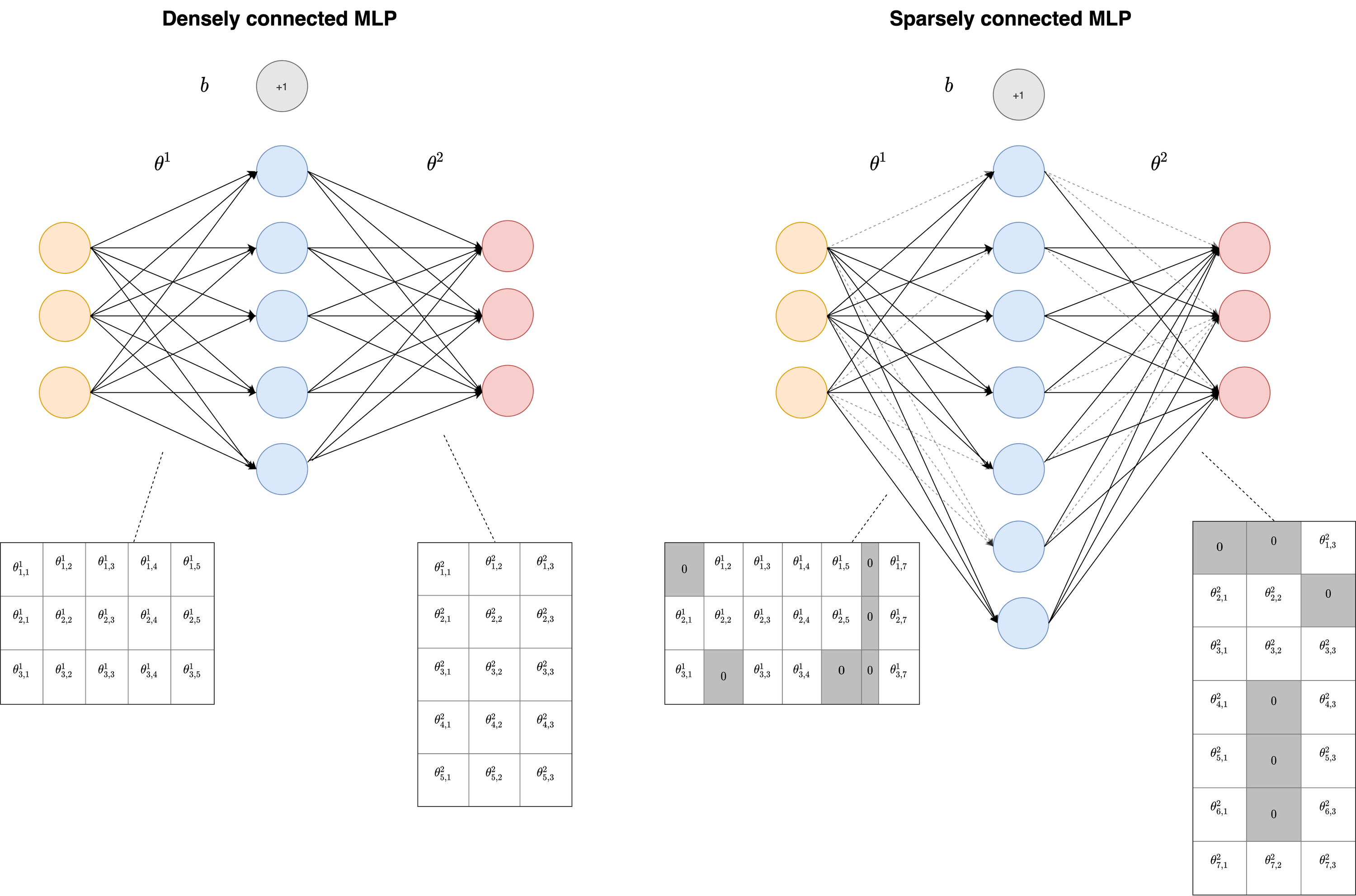
Figure 6: Fair Comparison of Sparse and Dense Networks. We fairly compare sparse and dense networks, by ensuring they have the same number of connections per layer and turning off the bias unit.

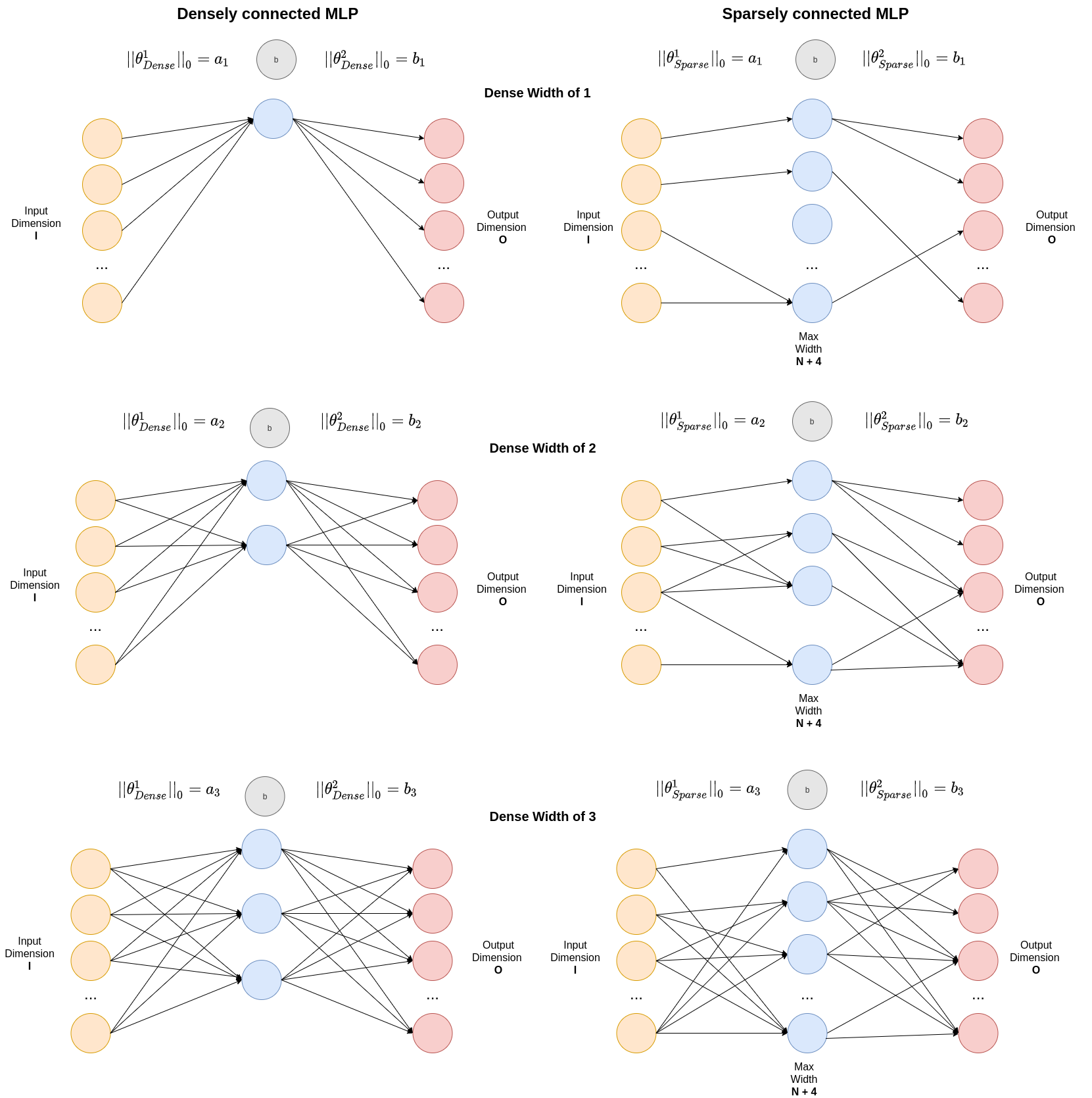
Figure 7: Fairly Comparing Sparse and Dense Networks at Different Widths. We show how we ensure that sparse and dense networks have the same parameter count, at different widths.

A.2 Benefits of SC-SDC

The benefits of SC-SDC can be summarized as follows:

• We can better understand sparse network optimization. SC-SDC allows us to identify which optimization or regularization methods are poorly suited to sparse networks in a controlled setting, ensuring the results are a direct result of the sparse connections themselves.

• Learn at what parameter and size budget, sparse networks are better than dense. Comparing sparse and dense networks of the same capacity allows us to see which architecture is better at different configurations. In configurations where sparse architectures perform better, we could exploit advances in sparse matrix computation and storage (Zhao et al., 2018; Merrill & Garland, 2016; Ma et al., 2019; Zhang et al., 2019b, 2020) to simply default to sparse architectures.

Appendix B Gradient Flow

In the main body of the paper, we use $EGF_{2}$ (Equation 6) as our notion of gradient flow for its comparative benefits with other measures of gradient flow. In this section, for completeness, we present the full set of results using the different formulations of gradient flow on CIFAR-100. Namely, we show $||{\bm{g}}||_{1}$ (Equation 5) (Figure 9 and 12) ,$||{\bm{g}}||_{2}$ (Equation 5) (Figure 10 and 13) and $EGF_{1}$ (Equation 6) (Figure 8 and 11).

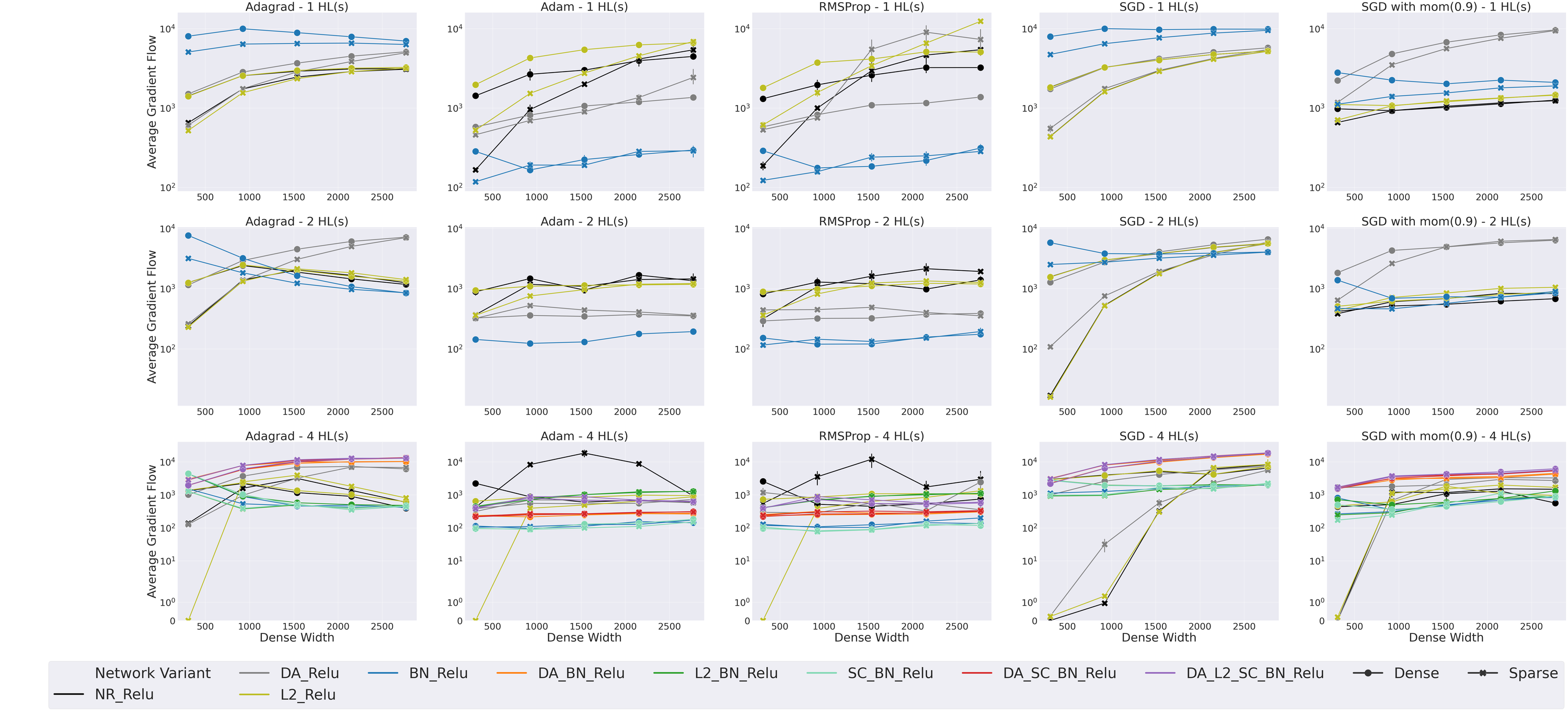
Figure 8: Gradient Flow in CIFAR-100 using $EGF_{1}$, with low learning rate (0.001)

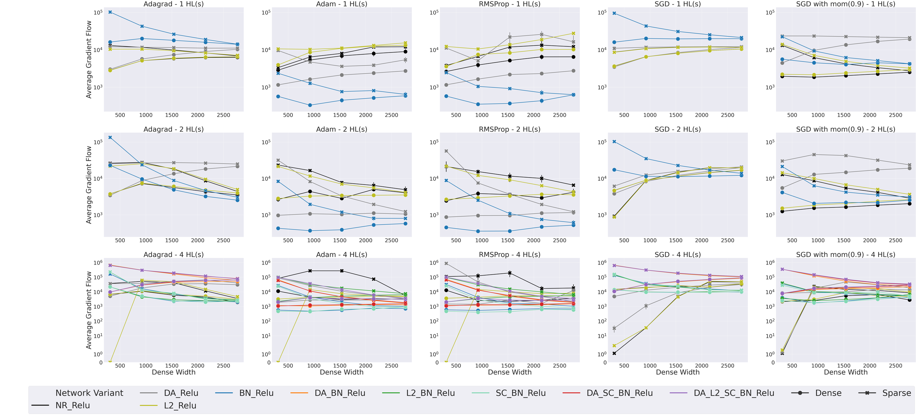
Figure 9: Gradient Flow in CIFAR-100 using $||{\bm{g}}||_{1}$, with low learning rate (0.001)

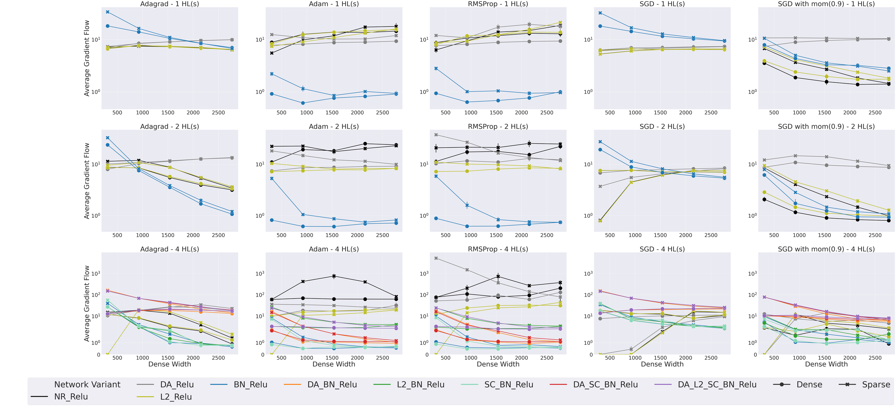
Figure 10: Gradient Flow in CIFAR-100 using $||{\bm{g}}||_{2}$ , with low learning rate (0.001)

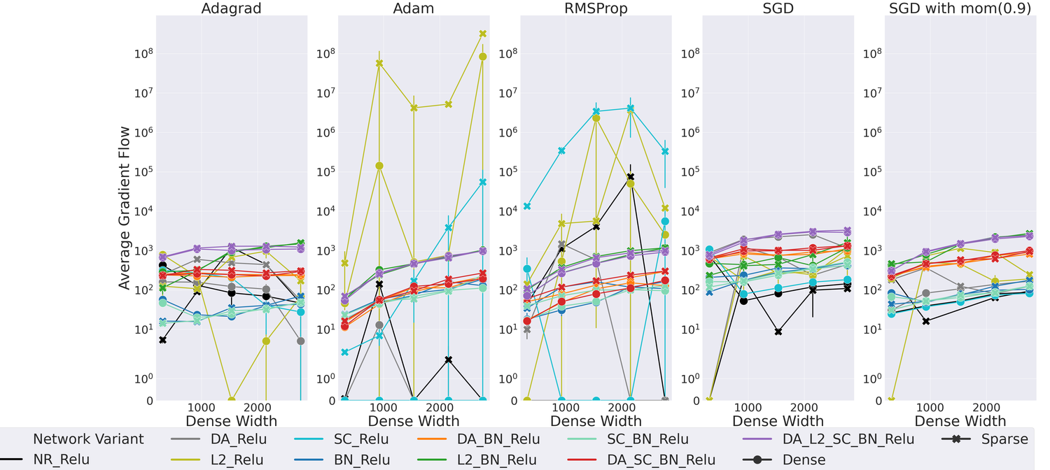
Figure 11: Gradient Flow in CIFAR-100 using $EGF_{1}$, with high learning rate (0.1)

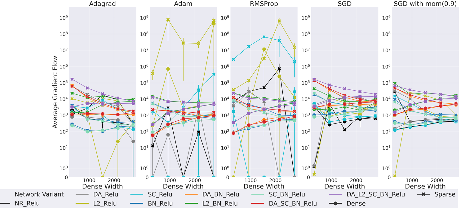
Figure 12: Gradient Flow in CIFAR-100 using $||{\bm{g}}||_{1}$, with high learning rate (0.1)

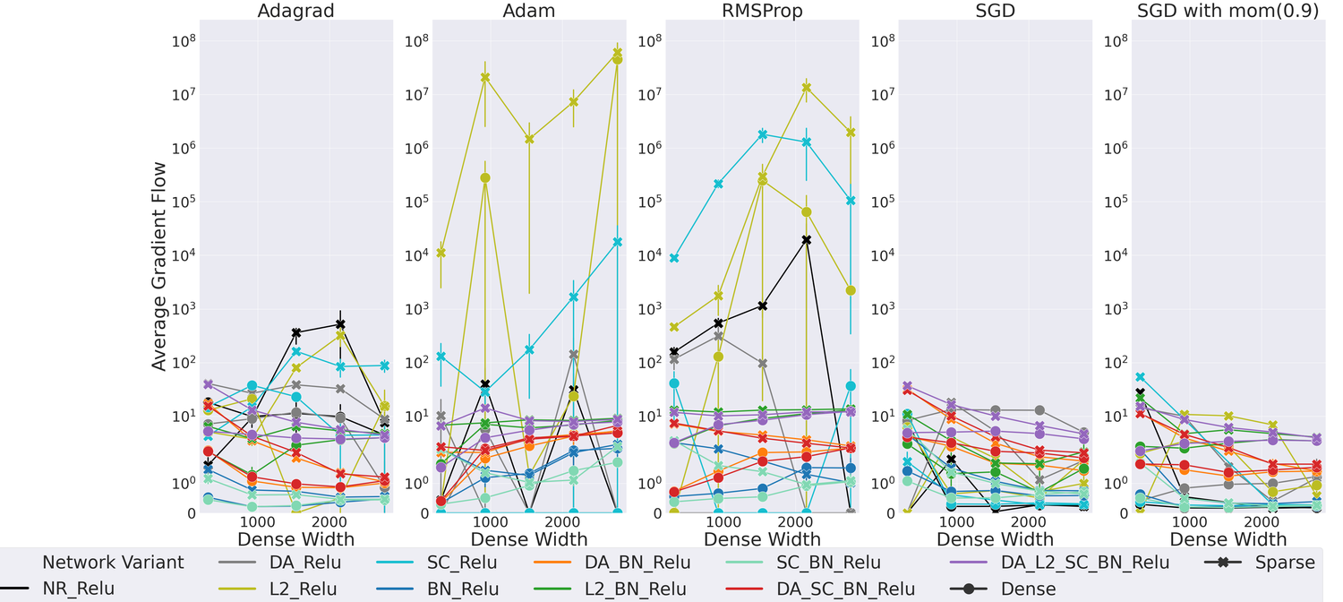
Figure 13: Gradient Flow in CIFAR-100 using $||{\bm{g}}||_{2}$ , with high learning rate (0.1)

Appendix C Adaptive Methods

Not all adaptive methods are created equally. We briefly show the different update rules of the adaptive learning rate methods we use in our experiments. In Equations 13, we highlight that Adam and RMSProp have the same second moment estimate $\displaystyle\mathbf{v}_{t}$, which uses an exponential weighted moving average (EWMA) of past squared gradients to obtain an estimate of the variance of the gradient, which differs from Adagrad’s $\displaystyle\mathbf{v}_{t}$.

$$\begin{array}[]{lll}\text{Adagrad}&\qquad\text{RMSProp}&\qquad\text{Adam}\\ \hbox{\pagecolor{orange}$\displaystyle\mathbf{v}_{t}=\mathbf{v}_{t-1}+\mathbf{g}_{t}^{2}$}&\qquad\hbox{\pagecolor{yellow}$\displaystyle\mathbf{v}_{t}=\gamma\mathbf{v}_{t-1}+(1-\gamma)\mathbf{g}_{t}^{2}$}&\qquad\mathbf{m}_{t}=\beta_{1}\mathbf{m}_{t-1}+\left(1-\beta_{1}\right)\mathbf{g}_{t}\\ \mathbf{w}_{t}=\mathbf{w}_{t-1}-\dfrac{\eta}{\sqrt{\mathbf{v}_{t}+\epsilon}}\odot\mathbf{g}_{t}&\qquad\mathbf{w}_{t}=\mathbf{w}_{t-1}-\dfrac{\eta}{\sqrt{\mathbf{v}_{t}+\epsilon}}\odot\mathbf{g}_{t}&\qquad\hbox{\pagecolor{yellow}$\displaystyle\mathbf{v}_{t}=\beta_{2}\mathbf{v}_{t-1}+\left(1-\beta_{2}\right)\mathbf{g}_{t}^{2}$}\\ &&\qquad\mathbf{m}_{t}=\dfrac{\mathbf{m}_{t}}{1-\beta_{1}}\\ &&\qquad\mathbf{v}_{t}=\dfrac{\mathbf{v}_{t}}{1-\beta_{2}}\\ &&\qquad\mathbf{g}_{t}^{\prime}=\dfrac{\eta\hat{\mathbf{m}}_{t}}{\sqrt{\hat{\mathbf{v}}_{t}}+\epsilon}\\ &&\qquad\mathbf{w}_{t}=\mathbf{w}_{t-1}-\mathbf{g}_{t}^{\prime}\\ \end{array}$$ (13)

where $\displaystyle\mathbf{g}_{t}$ are the gradients of a network, $\displaystyle\mathbf{m}_{t}$ is the estimate of the first moment of the gradient, $\displaystyle\mathbf{v}_{t}$ is the estimate of the second moment of the gradient, $\displaystyle\eta$ is the learning rate, $\displaystyle\beta_{1}$,$\displaystyle\beta_{2}$,$\displaystyle\gamma$ are weighting parameters.

This difference between EWMA optimizers (Adam and RMSProp) and Adagrad is two-fold:

1. Adagrad’s $\displaystyle\mathbf{v}_{t}$ is evenly weighted between the current squared gradient $\mathbf{{g}_{t}^{2}}$ and the previous value of $\mathbf{v}_{t}$. Adam and RMSProp’s $\displaystyle\mathbf{v}_{t}$ use $0.9$ (Hinton et al., 2012) or $0.999$ (Kingma & Ba, 2014) as a weighting parameter for the past $\mathbf{v}_{t}$, which weights past $\mathbf{v}_{t-1}$ more than $\mathbf{g}_{t}$.

2. Adagrad’s $\displaystyle\mathbf{v}_{t}$ grows almost linearly over time (Zhang et al., 2019a), which results in fast decline in learning rate (a higher $\mathbf{v}_{t}$ results in a smaller effective learning rate since $\eta$ is divided by $\mathbf{v}_{t}$). Since Adam and RMSProp’s $\displaystyle\mathbf{v}_{t}$ is multiplied by a weighting factor, this value decreases over time. This occurs even if we choose a weighting factor of $0.5$, since both $\mathbf{v}_{t}$ and $\mathbf{g}_{t}$ will be multiplied by $0.5$. A smaller $\displaystyle\mathbf{v}_{t}$, results in a higher effective learning rate, meaning learning rates stay higher for longer.

We believe the higher effective learning rate (point 2) is why Adam and RMSProp behave similarly in some contexts. Furthermore, it has been noted that at times, when the $\displaystyle\mathbf{v}_{t}$ estimate blows up, it can cause optimizers to fail to converge (Zaheer et al., 2018; Zhang et al., 2019a). $\displaystyle\mathbf{v}_{t}$ is also present in the formulation of Adadelta (Zeiler, 2012).

Appendix D Activation Functions

We plot the activation functions we used (Figure 14(a)) and their gradients (Figure 14(b)).

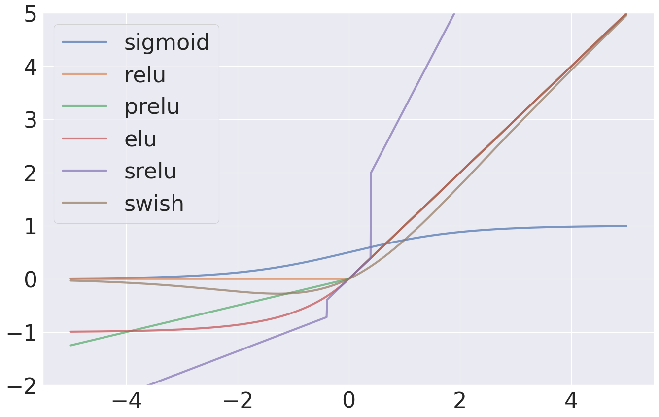
(a) Activation Function with inputs [-5,5]

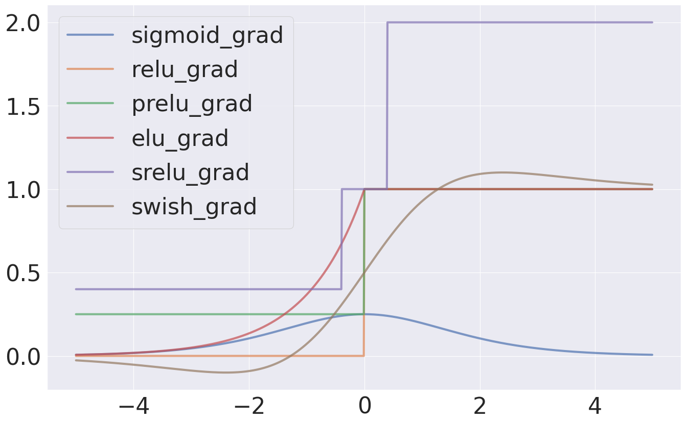
(b) Derivative of Activation Function with inputs [-5,5]

Figure 14: Plot of Activation Functions. We plot the activation functions we used and their derivatives. We see that Swish is the only activation function that allows for the flow of negative gradients, due its non-monotonicity.

Appendix E Detailed Results for SC-SDC

In this section, we present the detailed results for our experiments. For the tables, we use the following colour scale, depending on the p-value from the Wilcoxon Signed Rank Test.

Colour Scale based on p-values: 0 .5 1 S $>$ D S $\leq$ D

where $S$ refers to sparse networks and $D$ refers to dense networks.

E.1 Detailed Results

We present the detailed results as follows:

1. FMNIST

   1. All SC-SDC results for Four Hidden Layers with different regularization methods - Table 4.

   2. Effects of Regularization with a low learning rate (0.001) - Figure 15.

2. CIFAR-10

   1. All SC-SDC results for Four Hidden Layers with different regularization methods - Table 5.

   2. Effects of Regularization with a low learning rate (0.001) - Figure 16.

   3. Effects of Regularization with a high learning rate (0.1) - Figure 17.

   4. Effects of Activations with a low learning rate (0.001) - Figure 18.

3. CIFAR-100

   1. Detailed Results with a low learning rate (0.001)

      1. One, Two and Four hidden layers showing all forms of regularization - accuracy and gradient flow (Figure 19).

      2. Four Hidden Layers with different activation functions - accuracy and gradient flow (Figure 20).

      3. All SC-SDC results for Four Hidden Layers with different regularization and activation methods- Table 6.

   2. Detailed Results with a high learning rate (0.1)

      1. Four Hidden Layers with BatchNorm - accuracy and gradient flow (Figure 21).

      2. Four Hidden Layers with different activation functions - accuracy and gradient flow (Figure 22).

      3. Adam vs AdamW - accuracy and gradient flow (Figure 23).

      4. Gradient Flow for Wide ResNet-50 - Figure 24.

	NR_Relu	L2_Relu	DA_Relu	SC_Relu	BN_Relu	DA_SC_BN_Relu	DA_L2_SC_BN_Relu
Adagrad	0.993	0.992	1.000	0.941	0.001	0.001	0.000
Adam	0.170	0.995	0.088	0.012	0.020	0.000	0.076
Mom (0.9)	1.000	0.991	1.000	0.924	0.000	0.008	0.008

Table 4: Wilcoxon Signed Rank Test Results for MLPs With Four Hidden Layers, With a Low Learning Rate (0.001), trained on FMNIST.

Figure 15: Effect of Regularization on Accuracy and Gradient Flow for Dense and Sparse Networks, with Four Hidden Layers on FMNIST, with low learning rate (0.001)

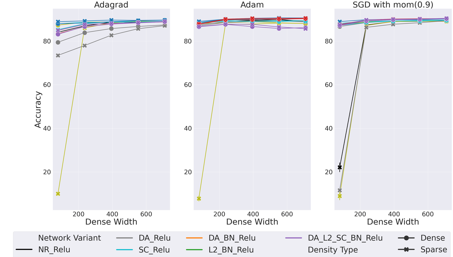
(a) Test Accuracy for Dense and Sparse Networks on FMNIST

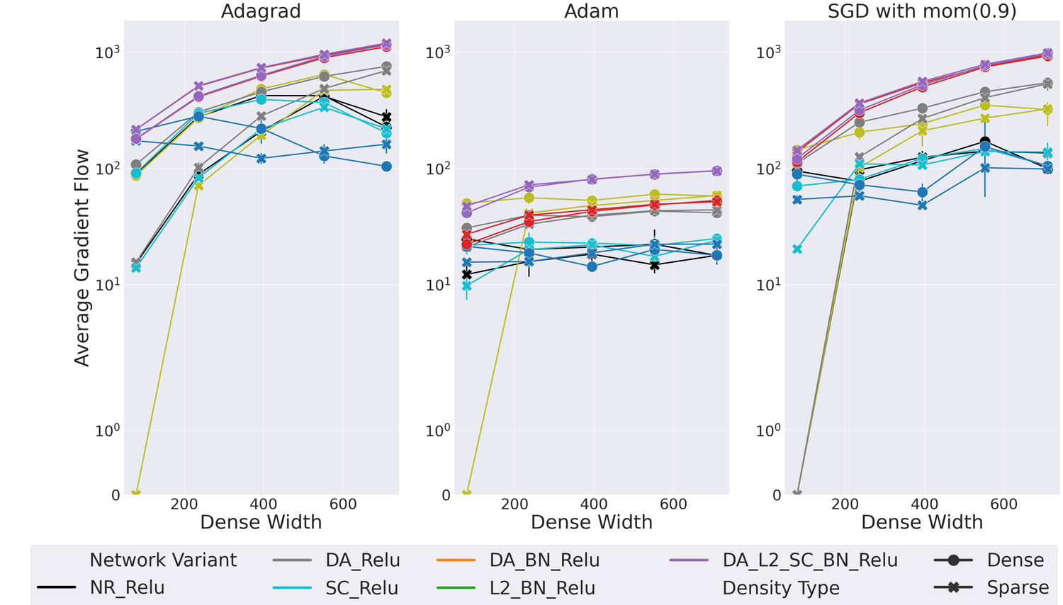
(b) Gradient Flow for Dense and Sparse Networks on FMNIST

(a) Different Regularization Methods - Low learning rate (0.001)

	NR	DA	L2	SC	BN
Adagrad	0.555	0.681	0.999	0.271	0.000
Adam	0.024	0.001	0.681	0.000	0.000
RMSProp	0.000	0.598	0.866	0.001	0.005
SGD	1.000	1.000	1.000	0.000	0.000
Mom (0.9)	1.000	0.862	1.000	0.995	0.001

(b) Different Regularization Methods - High learning rate (0.1)

	BN	DA_BN	L2_BN	SC_BN
Adagrad	0.001	0.063	0.953	0.000
Adam	0.009	0.001	0.074	0.000
RMSProp	0.227	0.375	0.219	0.037
SGD	0.000	0.500	0.289	0.000
Mom (0.9)	0.000	0.024	0.004	0.000

(c) Effect of Different Activation Functions - High learning rate (0.001)

	ReLU	SReLU	Swish	PReLU
Adam	0.004	0.006	0.002	0.005
Mom (0.9)	0.000	0.053	0.002	0.001

Table 5: Wilcoxon Signed Rank Test Results for MLPs with Four Hidden Layers, trained on CIFAR-10. Wilcoxon Signed Rank Test Results for CIFAR-10, using a $p$-value of 0.05, with the bold values indicating where we can be statistically confident that sparse networks perform better than dense (reject $H_{0}$ from 4). We also use a continuous colour scale to make the results more interpretable. This scale ranges from green (0 - likely that sparse networks perform better than dense) to yellow (0.5 - 50% chance that sparse networks perform better than dense) to red (1 - highly likely that sparse networks do not outperform dense - cannot reject $H_{0}$ from 4).

Figure 16: Effect of Regularization on Accuracy and Gradient Flow for Dense and Sparse Networks, on CIFAR-10, with low learning rate (0.001)

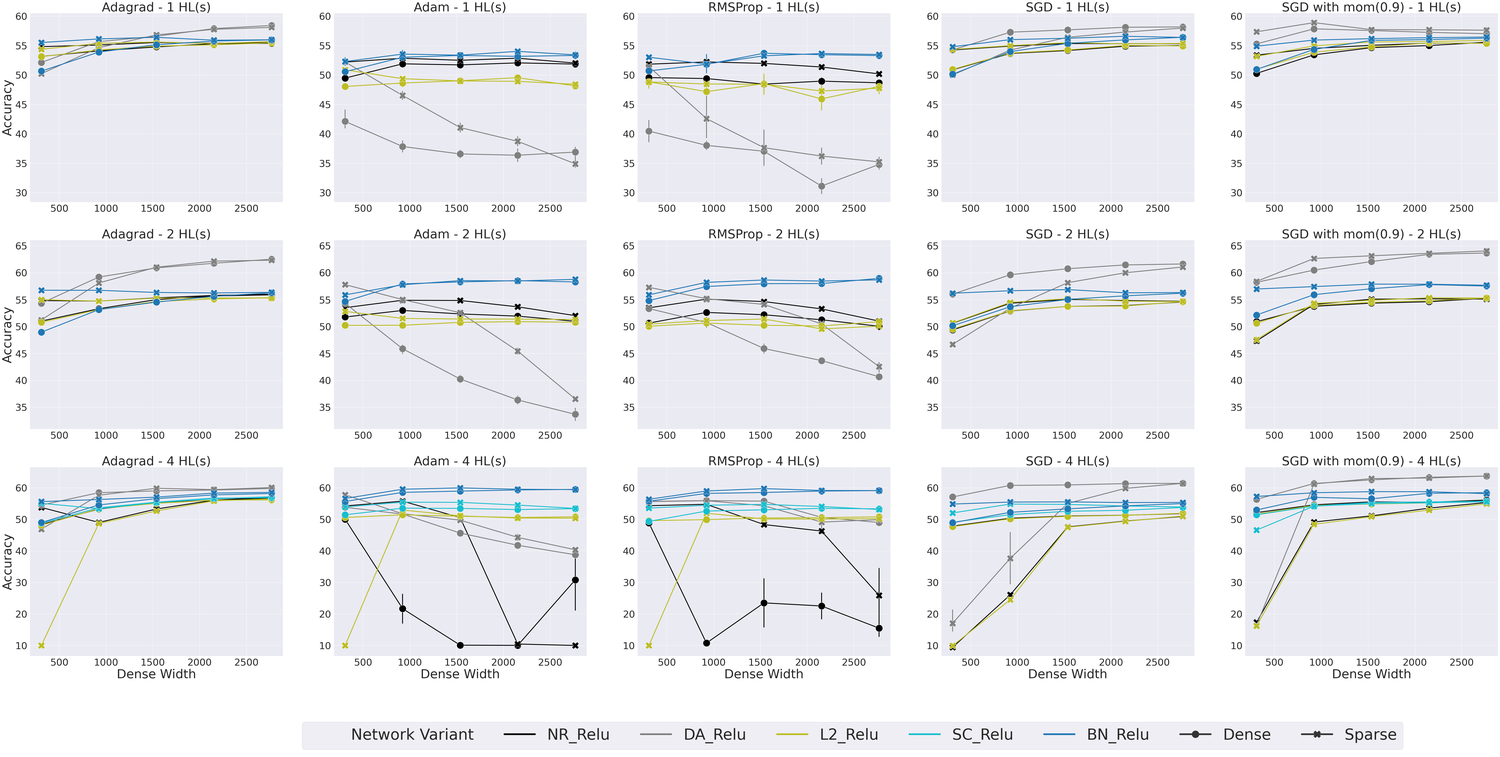
(d) Test Accuracy for Dense and Sparse Networks

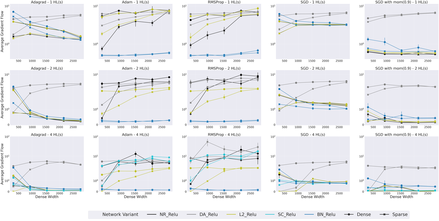
(e) Gradient Flow for Dense and Sparse Networks

Figure 17: Effect of Regularization on Accuracy and Gradient Flow for Dense and Sparse Networks, with Four Hidden Layers on CIFAR-10, with high learning rate (0.1)

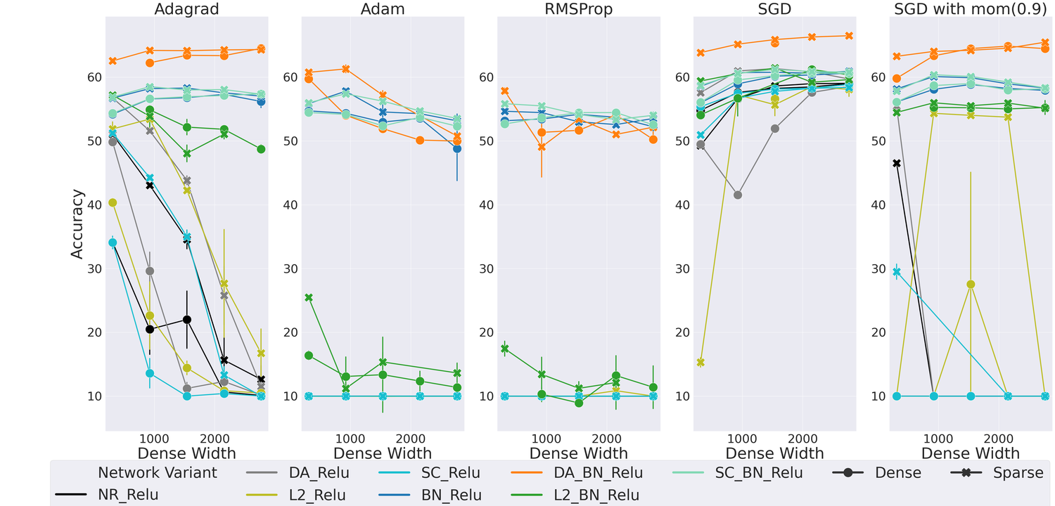
(f) Test Accuracy for Dense and Sparse Networks

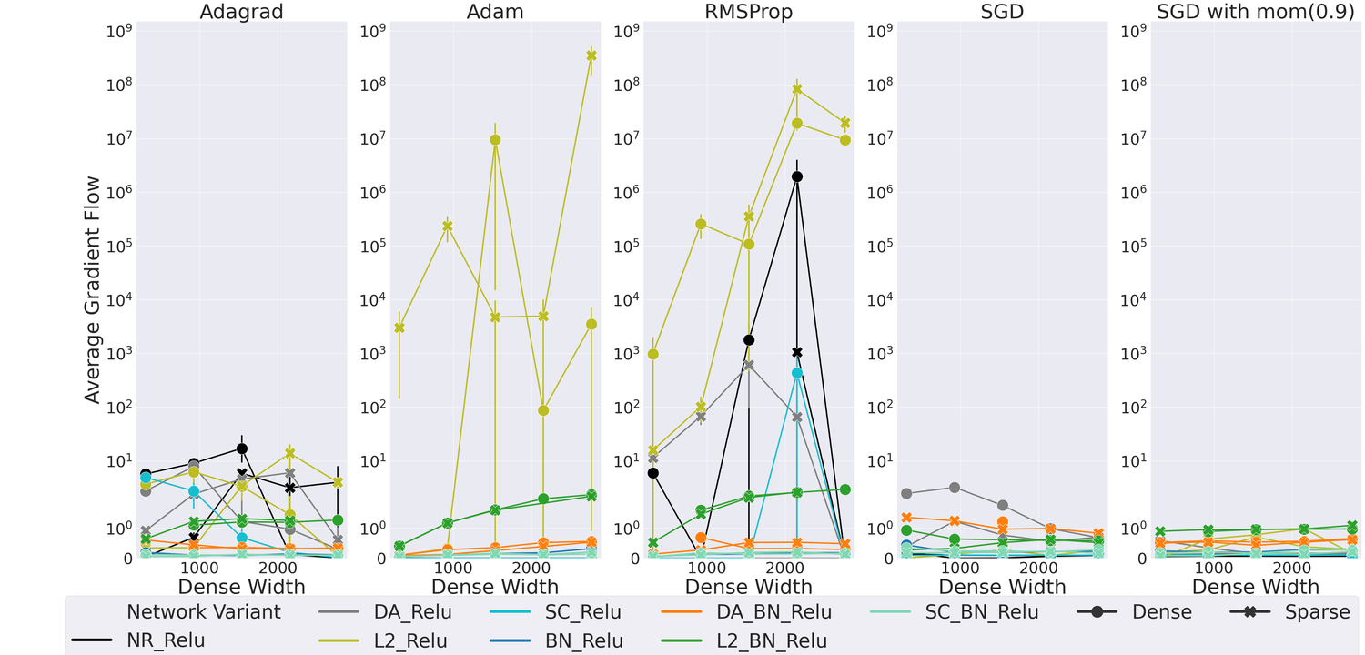
(g) Gradient Flow for Dense and Sparse Networks

Figure 18: Effect of Activation Functions on Accuracy and Gradient Flow for Dense and Sparse Networks with Four Hidden Layers on CIFAR-10, with low learning rate (0.001)

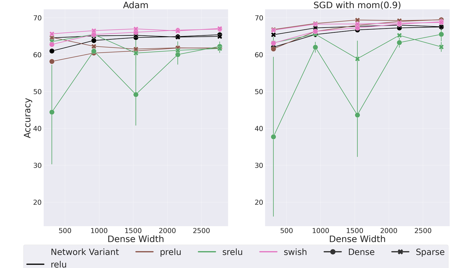
(a) Test Accuracy for Dense and Sparse Networks on CIFAR-10

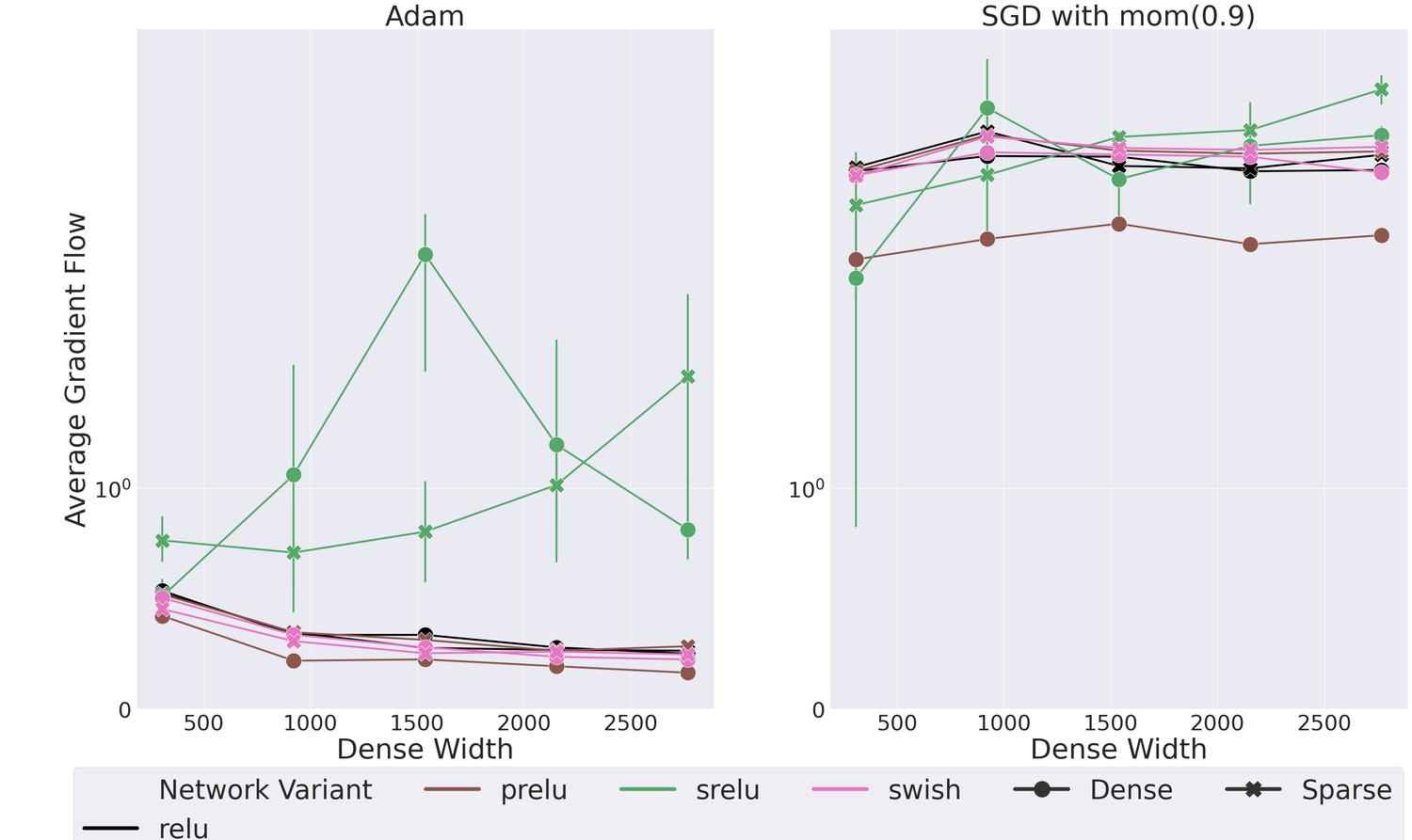
(b) Gradient Flow for Dense and Sparse Networks on CIFAR-10

Figure 19: Effect of Regularization on Accuracy and Gradient Flow for Dense and Sparse Networks with One, Two and Four Hidden Layers on CIFAR-100, with low learning rate (0.001)

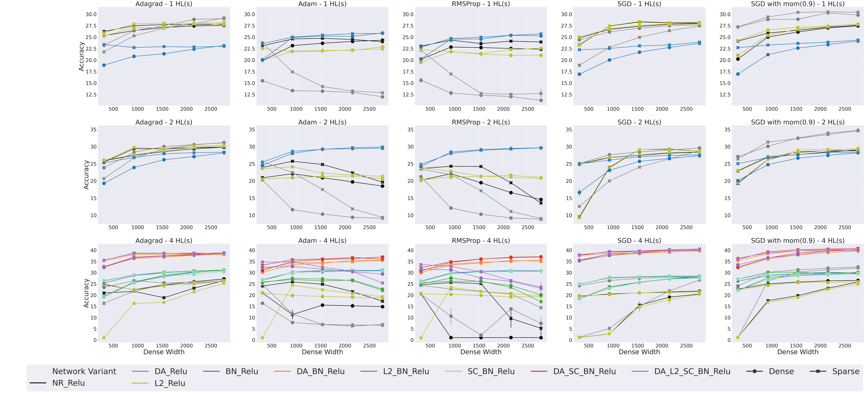
(h) Test Accuracy for Dense and Sparse Networks on CIFAR-100

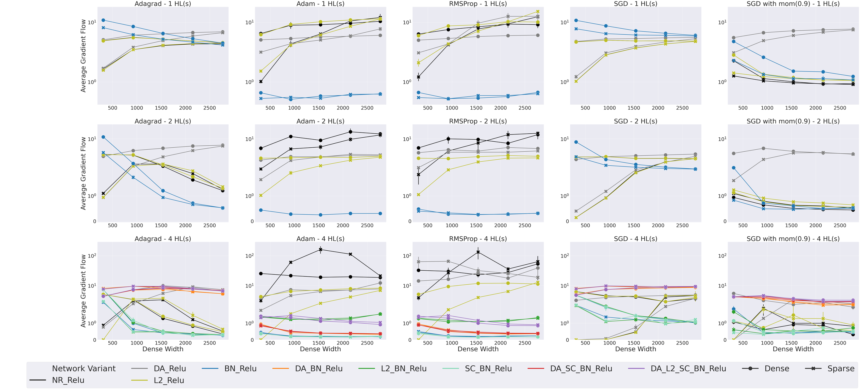
(i) Gradient Flow for Dense and Sparse Networks on CIFAR-100

Figure 20: Effect of Activation Functions on Accuracy and Gradient Flow for Dense and Sparse Networks with Four Hidden Layers on CIFAR-100, with low learning rate (0.001)

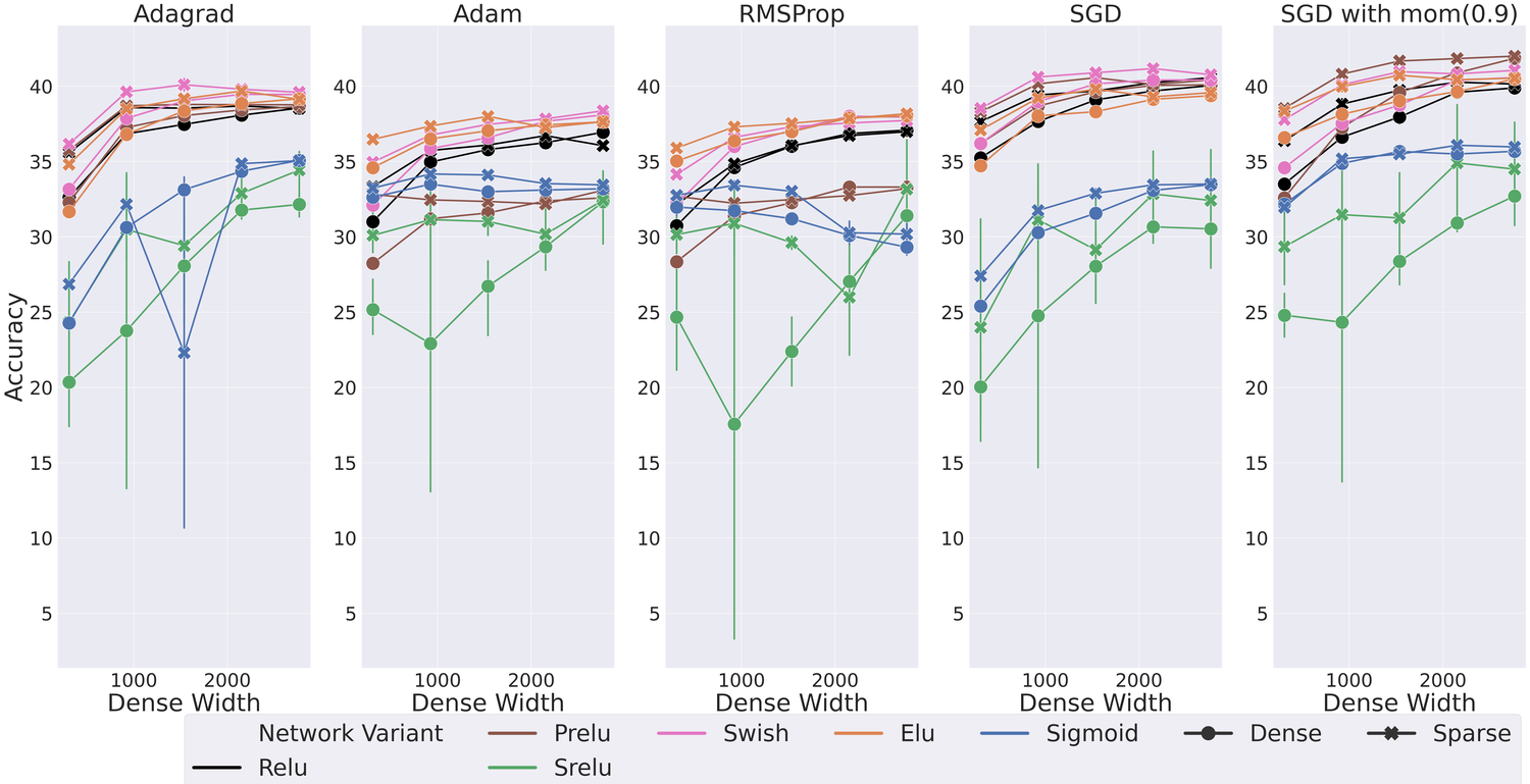
(j) Test Accuracy for Dense and Sparse Networks on CIFAR-100

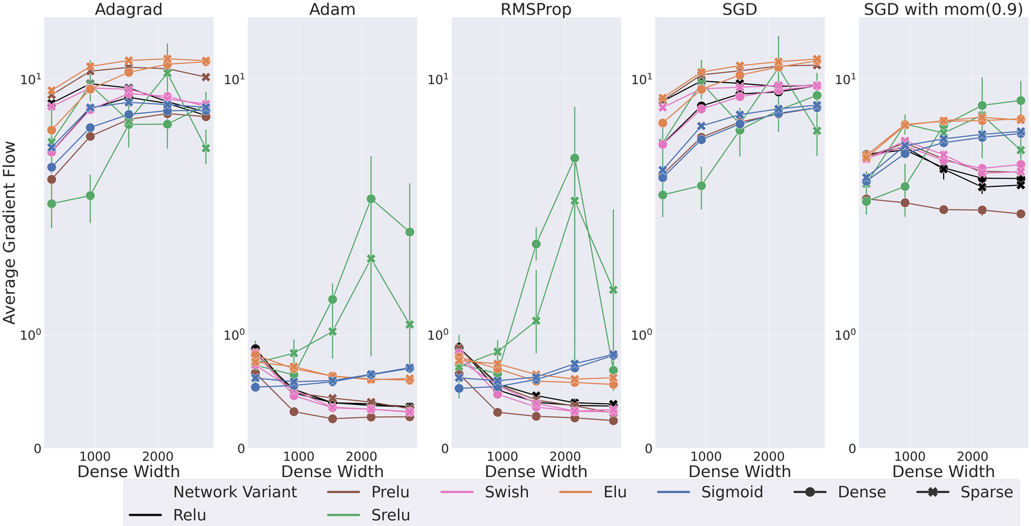
(k) Gradient Flow for Dense and Sparse Networks on CIFAR-100

(a) Effect of Different Regularization Methods

	NR	DA	L2	SC	BN	DA_BN	L2_BN	SC_BN	DA_SC_BN	DA_L2_SC_BN
Adagrad	1.000	1.000	0.998	0.239	0.006	0.002	0.001	0.003	0.001	0.004
Adam	0.000	0.055	0.198	0.003	0.079	0.051	0.254	0.166	0.039	0.118
RMSProp	0.001	0.000	0.300	0.166	0.117	0.021	0.914	0.541	0.096	0.023
SGD	1.000	1.000	1.000	0.248	0.000	0.000	0.001	0.003	0.001	0.004
Mom (0.9)	1.000	1.000	1.000	0.999	0.001	0.000	0.007	0.008	0.001	0.003

(b) Effect of Activation Functions

	relu	swish	srelu	prelu	elu	sigmoid
Adagrad	0.000	0.001	0.104	0.001	0.000	0.011
Adam	0.042	0.003	0.076	0.001	0.004	0.000
RMSProp	0.104	0.165	0.065	0.047	0.013	0.001
SGD	0.002	0.000	0.180	0.000	0.001	0.000
Mom (0.9)	0.001	0.000	0.054	0.000	0.000	0.054

Table 6: Wilcoxon Signed Rank Test Results for MLPs with Four Hidden Layers, with low learning rate (0.001), trained on CIFAR-100. Wilcoxon Signed Rank Test Results for CIFAR-100, using a low learning rate. We use a $p$-value of 0.05, with the bold values indicating where we can be statistically confident that sparse networks perform better than dense (reject $H_{0}$ from 4). We also use a continuous colour scale to make the results more interpretable. This scale ranges from green (0 - likely that sparse networks perform better than dense) to yellow (0.5 - 50% chance that sparse networks perform better than dense) to red (1 - highly likely that sparse networks do not outperform dense - cannot reject $H_{0}$ from 4).

Figure 21: Effect of Regularization (with BatchNorm) on Accuracy and Gradient Flow for Dense and Sparse Networks, with Four Hidden Layers on CIFAR-100, with high learning rate (0.1)

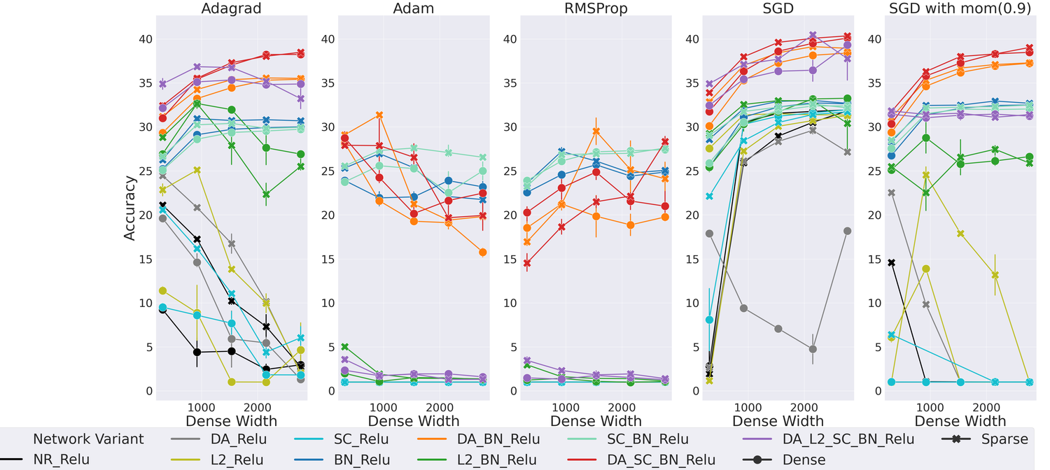
(c) Test Accuracy for Dense and Sparse Networks on CIFAR-100

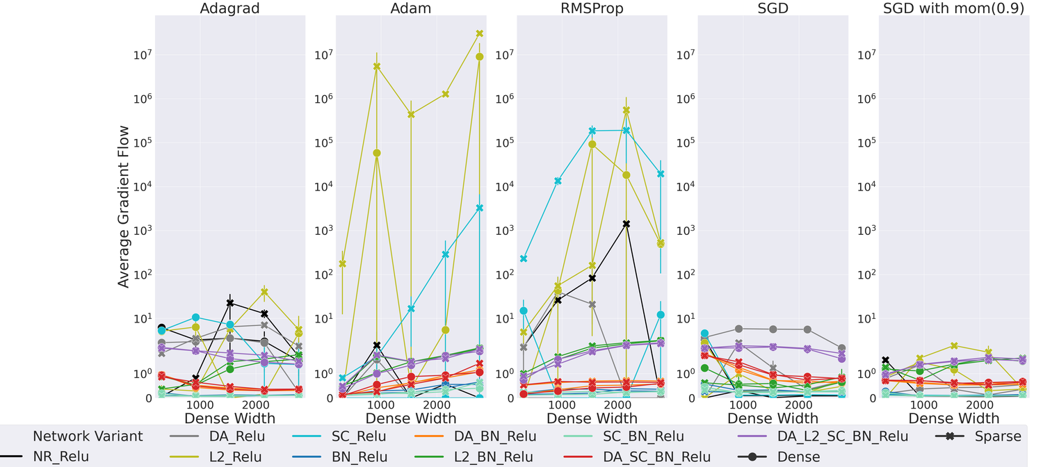
(d) Gradient Flow for Dense and Sparse Networks on CIFAR-100

Figure 22: Effect of Activation Functions on Accuracy and Gradient Flow for Dense and Sparse Networks with Four Hidden Layers on CIFAR-100, with high learning rate (0.1)

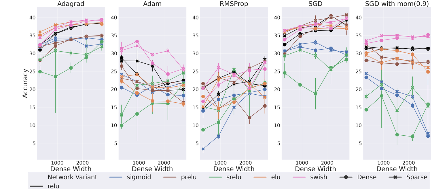
(e) Test Accuracy for Dense and Sparse Networks on CIFAR-100

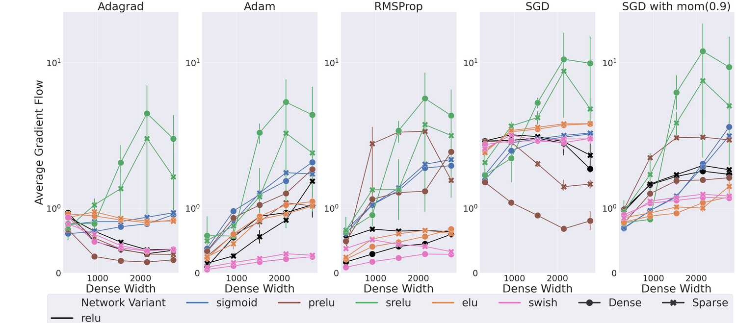
(f) Gradient Flow for Dense and Sparse Networks on CIFAR-100

Figure 23: Comparison of Adam and AdamW for Dense and Sparse Networks. We compare the performance of Adam and AdamW for dense and sparse Networks with four hidden layers on CIFAR-100, with a high learning rate (0.1). We see that AdamW’s weight decay formulation has a lower EGF than the standard L2 formulation used in Adam and this correlates to better network performance in AdamW

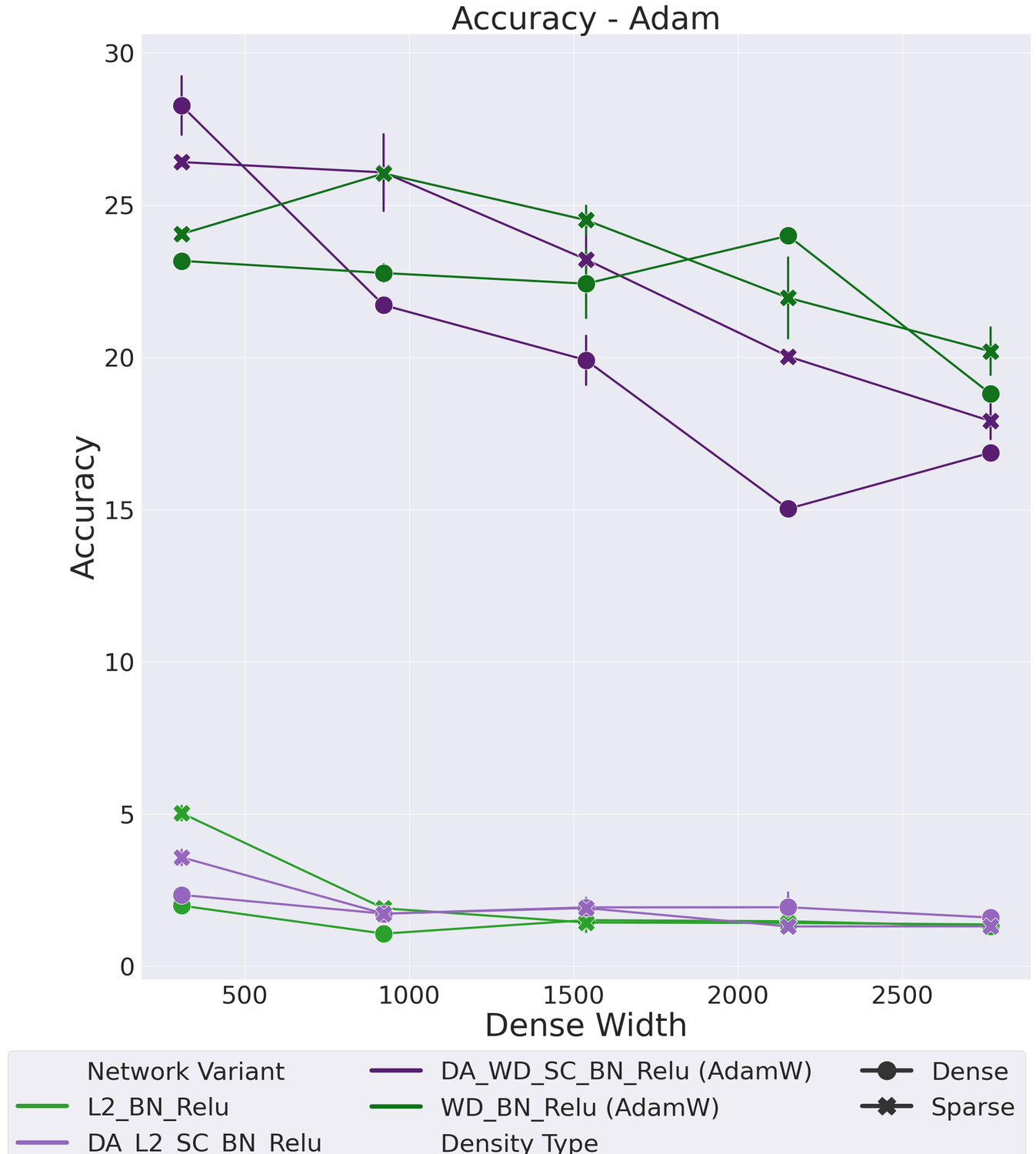
(a) Test Accuracy for Dense and Sparse Networks on CIFAR-100

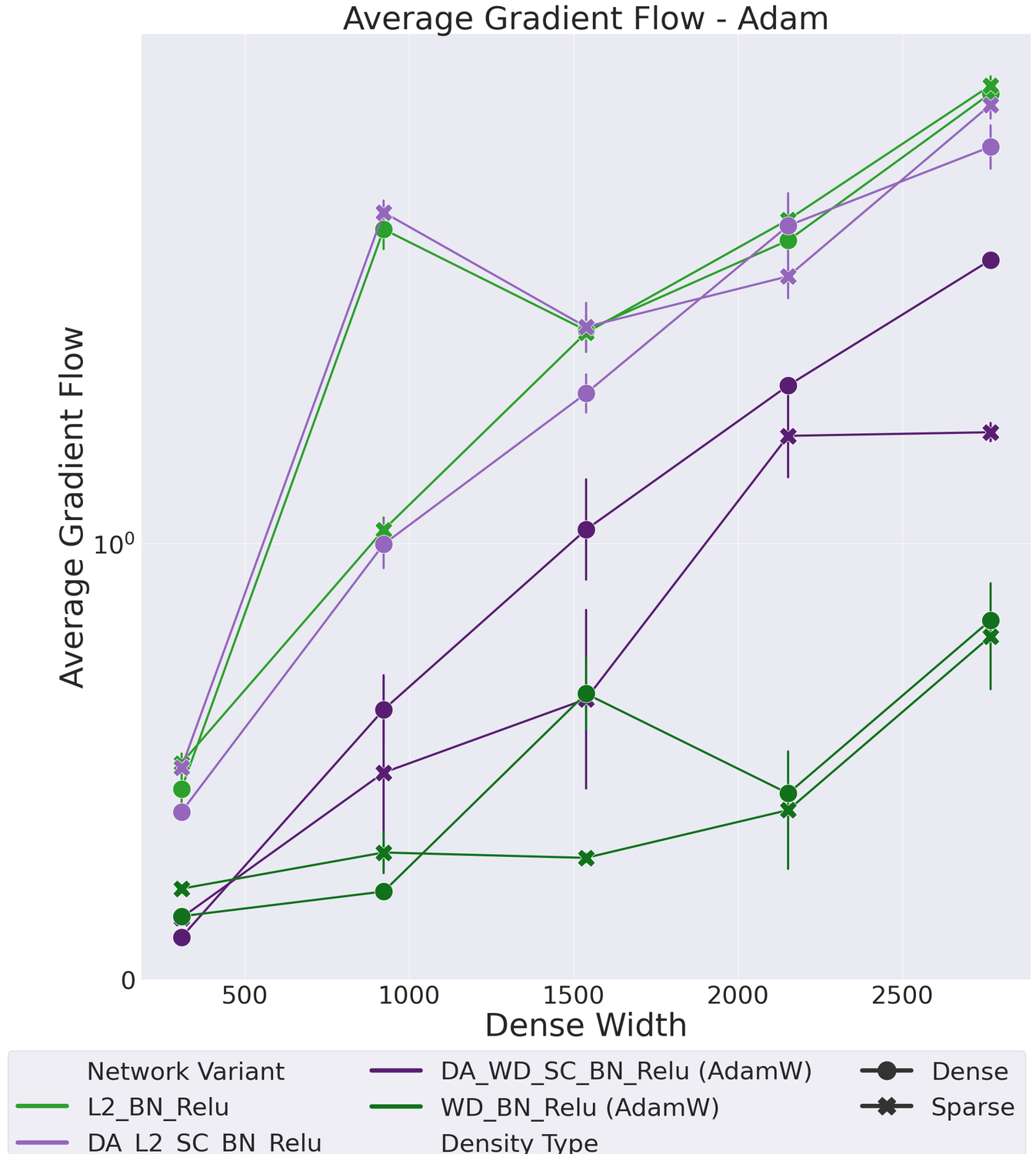
(b) Gradient Flow for Dense and Sparse Networks on CIFAR-100

References

- Ahmad & Scheinkman (2019) Subutai Ahmad and Luiz Scheinkman. How can we be so dense? the benefits of using highly sparse representations. arXiv preprint arXiv:1903.11257, 2019.
- Amodei et al. (2018) Dario Amodei, Danny Hernandez, Girish Sastry, Jack Clark, Greg Brockman, and Ilya Sutskever. Ai and compute, 2018. URL https://openai.com/blog/ai-and-compute/.
- Ba et al. (2016) Jimmy Lei Ba, Jamie Ryan Kiros, and Geoffrey E Hinton. Layer normalization. arXiv preprint arXiv:1607.06450, 2016.
- Balduzzi et al. (2017) David Balduzzi, Marcus Frean, Lennox Leary, JP Lewis, Kurt Wan-Duo Ma, and Brian McWilliams. The shattered gradients problem: If resnets are the answer, then what is the question? arXiv preprint arXiv:1702.08591, 2017.
- Bellec et al. (2017) Guillaume Bellec, David Kappel, Wolfgang Maass, and Robert Legenstein. Deep rewiring: Training very sparse deep networks. arXiv preprint arXiv:1711.05136, 2017.
- Bengio et al. (1994) Yoshua Bengio, Patrice Simard, and Paolo Frasconi. Learning long-term dependencies with gradient descent is difficult. IEEE transactions on neural networks, 5(2):157–166, 1994.
- Chen et al. (2018) Zhao Chen, Vijay Badrinarayanan, Chen-Yu Lee, and Andrew Rabinovich. Gradnorm: Gradient normalization for adaptive loss balancing in deep multitask networks. In International Conference on Machine Learning, pp. 794–803. PMLR, 2018.
- Clevert et al. (2015) Djork-Arné Clevert, Thomas Unterthiner, and Sepp Hochreiter. Fast and accurate deep network learning by exponential linear units (elus). arXiv preprint arXiv:1511.07289, 2015.
- Cun et al. (1990) Yann Le Cun, John S. Denker, and Sara A. Solla. Optimal brain damage. In Advances in Neural Information Processing Systems, pp. 598–605. Morgan Kaufmann, 1990.
- Demšar (2006) Janez Demšar. Statistical comparisons of classifiers over multiple data sets. Journal of Machine learning research, 7(Jan):1–30, 2006.
- Dettmers & Zettlemoyer (2019) Tim Dettmers and Luke Zettlemoyer. Sparse networks from scratch: Faster training without losing performance. arXiv preprint arXiv:1907.04840, 2019.
- Dubowski (2020) Adam Dubowski. Activation function impact on sparse neural networks. B.S. thesis, University of Twente, 2020.
- Duchi et al. (2011) John Duchi, Elad Hazan, and Yoram Singer. Adaptive subgradient methods for online learning and stochastic optimization. Journal of machine learning research, 12(7), 2011.
- Eldan & Shamir (2016) Ronen Eldan and Ohad Shamir. The power of depth for feedforward neural networks. In Conference on learning theory, pp. 907–940, 2016.
- Evci et al. (2019) Utku Evci, Trevor Gale, Jacob Menick, Pablo Samuel Castro, and Erich Elsen. Rigging the Lottery: Making All Tickets Winners. arXiv e-prints, art. arXiv:1911.11134, November 2019.
- Evci et al. (2019) Utku Evci, Fabian Pedregosa, Aidan Gomez, and Erich Elsen. The difficulty of training sparse neural networks. arXiv preprint arXiv:1906.10732, 2019.
- Evci et al. (2020) Utku Evci, Yani A Ioannou, Cem Keskin, and Yann Dauphin. Gradient flow in sparse neural networks and how lottery tickets win. arXiv preprint arXiv:2010.03533, 2020.
- Frankle & Carbin (2019) Jonathan Frankle and Michael Carbin. The lottery ticket hypothesis: Finding sparse, trainable neural networks. In International Conference on Learning Representations, 2019. URL https://openreview.net/forum?id=rJl-b3RcF7.
- Frankle et al. (2019a) Jonathan Frankle, Gintare Karolina Dziugaite, Daniel M Roy, and Michael Carbin. Linear mode connectivity and the lottery ticket hypothesis. arXiv preprint arXiv:1912.05671, 2019a.
- Frankle et al. (2019b) Jonathan Frankle, Gintare Karolina Dziugaite, Daniel M Roy, and Michael Carbin. Stabilizing the lottery ticket hypothesis. arXiv preprint arXiv:1903.01611, 2019b.
- Frankle et al. (2020) Jonathan Frankle, Gintare Karolina Dziugaite, Daniel M. Roy, and Michael Carbin. Pruning neural networks at initialization: Why are we missing the mark?, 2020.
- Funahashi (1989) Ken-Ichi Funahashi. On the approximate realization of continuous mappings by neural networks. Neural networks, 2(3):183–192, 1989.
- Gale et al. (2019) Trevor Gale, Erich Elsen, and Sara Hooker. The State of Sparsity in Deep Neural Networks. arXiv e-prints, art. arXiv:1902.09574, February 2019.
- Glorot & Bengio (2010) Xavier Glorot and Yoshua Bengio. Understanding the difficulty of training deep feedforward neural networks. In Proceedings of the thirteenth international conference on artificial intelligence and statistics, pp. 249–256, 2010.
- Glorot et al. (2011) Xavier Glorot, Antoine Bordes, and Yoshua Bengio. Deep sparse rectifier neural networks. In Proceedings of the fourteenth international conference on artificial intelligence and statistics, pp. 315–323, 2011.
- Goodfellow et al. (2016) Ian Goodfellow, Yoshua Bengio, Aaron Courville, and Yoshua Bengio. Deep learning, volume 1. MIT Press, 2016.
- Han et al. (2015) Song Han, Jeff Pool, John Tran, and William J. Dally. Learning both weights and connections for efficient neural networks. In Proceedings of the 28th International Conference on Neural Information Processing Systems - Volume 1, NIPS’15, pp. 1135–1143, Cambridge, MA, USA, 2015. MIT Press. URL http://dl.acm.org/citation.cfm?id=2969239.2969366.
- Hanson & Pratt (1989) Stephen José Hanson and Lorien Y Pratt. Comparing biases for minimal network construction with back-propagation. In Advances in neural information processing systems, pp. 177–185, 1989.
- Hassibi et al. (1993a) B. Hassibi, D. G. Stork, and G. J. Wolff. Optimal brain surgeon and general network pruning. In IEEE International Conference on Neural Networks, pp. 293–299 vol.1, March 1993a. doi: 10.1109/ICNN.1993.298572.
- Hassibi et al. (1993b) Babak Hassibi, David G. Stork, and Stork Crc. Ricoh. Com. Second order derivatives for network pruning: Optimal brain surgeon. In Advances in Neural Information Processing Systems 5, pp. 164–171. Morgan Kaufmann, 1993b.
- He et al. (2015) Kaiming He, Xiangyu Zhang, Shaoqing Ren, and Jian Sun. Delving deep into rectifiers: Surpassing human-level performance on imagenet classification. In Proceedings of the IEEE international conference on computer vision, pp. 1026–1034, 2015.
- He et al. (2016) Kaiming He, Xiangyu Zhang, Shaoqing Ren, and Jian Sun. Deep residual learning for image recognition. In Proceedings of the IEEE conference on computer vision and pattern recognition, pp. 770–778, 2016.
- Hinton et al. (2012) Geoffrey Hinton, Nitish Srivastava, and Kevin Swersky. Neural networks for machine learning lecture 6a overview of mini-batch gradient descent. Cited on, 14(8), 2012.
- Hochreiter (1991) Sepp Hochreiter. Untersuchungen zu dynamischen neuronalen netzen. Diploma, Technische Universität München, 91(1), 1991.
- Hochreiter et al. (2001) Sepp Hochreiter, Yoshua Bengio, Paolo Frasconi, Jürgen Schmidhuber, et al. Gradient flow in recurrent nets: the difficulty of learning long-term dependencies, 2001.
- Hooker et al. (2019) Sara Hooker, Aaron Courville, Gregory Clark, Yann Dauphin, and Andrea Frome. What Do Compressed Deep Neural Networks Forget? arXiv e-prints, art. arXiv:1911.05248, November 2019.
- Hornik et al. (1989) Kurt Hornik, Maxwell Stinchcombe, Halbert White, et al. Multilayer feedforward networks are universal approximators. Neural networks, 2(5):359–366, 1989.
- Horowitz (2014) M. Horowitz. 1.1 computing’s energy problem (and what we can do about it). In 2014 IEEE International Solid-State Circuits Conference Digest of Technical Papers (ISSCC), pp. 10–14, 2014.
- Ioffe & Szegedy (2015) Sergey Ioffe and Christian Szegedy. Batch normalization: Accelerating deep network training by reducing internal covariate shift. CoRR, abs/1502.03167, 2015. URL http://arxiv.org/abs/1502.03167.
- Jiang et al. (2019) Yiding Jiang, Behnam Neyshabur, Hossein Mobahi, Dilip Krishnan, and Samy Bengio. Fantastic generalization measures and where to find them. arXiv preprint arXiv:1912.02178, 2019.
- Jin et al. (2015) Xiaojie Jin, Chunyan Xu, Jiashi Feng, Yunchao Wei, Junjun Xiong, and Shuicheng Yan. Deep learning with s-shaped rectified linear activation units. arXiv preprint arXiv:1512.07030, 2015.
- Karnin (1990) Ehud D Karnin. A simple procedure for pruning back-propagation trained neural networks. IEEE transactions on neural networks, 1(2):239–242, 1990.
- Kendall (1938) Maurice G Kendall. A new measure of rank correlation. Biometrika, 30(1/2):81–93, 1938.
- Kingma & Ba (2014) Diederik P Kingma and Jimmy Ba. Adam: A method for stochastic optimization. arXiv preprint arXiv:1412.6980, 2014.
- Krizhevsky et al. (2009) Alex Krizhevsky, Vinod Nair, and Geoffrey Hinton. Cifar-10 and cifar-100 datasets. URl: https://www. cs. toronto. edu/kriz/cifar. html, 6:1, 2009.
- Krizhevsky et al. (2012) Alex Krizhevsky, Ilya Sutskever, and Geoffrey E Hinton. Imagenet classification with deep convolutional neural networks. In Advances in neural information processing systems, pp. 1097–1105, 2012.
- Krogh & Hertz (1992) Anders Krogh and John A Hertz. A simple weight decay can improve generalization. In Advances in neural information processing systems, pp. 950–957, 1992.
- Labatie (2019) Antoine Labatie. Characterizing well-behaved vs. pathological deep neural networks. In International Conference on Machine Learning, pp. 3611–3621. PMLR, 2019.
- Lane & Warden (2018) N. D. Lane and P. Warden. The deep (learning) transformation of mobile and embedded computing. Computer, 51(5):12–16, May 2018. ISSN 1558-0814. doi: 10.1109/MC.2018.2381129.
- LeCun et al. (1989) Yann LeCun, John S. Denker, and Sara A. Solla. Optimal Brain Damage. In NIPS, pp. 598–605. Morgan Kaufmann, 1989.
- Lee et al. (2018) Namhoon Lee, Thalaiyasingam Ajanthan, and Philip HS Torr. Snip: Single-shot network pruning based on connection sensitivity. arXiv preprint arXiv:1810.02340, 2018.
- Lee et al. (2019) Namhoon Lee, Thalaiyasingam Ajanthan, Stephen Gould, and Philip HS Torr. A signal propagation perspective for pruning neural networks at initialization. arXiv preprint arXiv:1906.06307, 2019.
- Liu & Zenke (2020) Tianlin Liu and Friedemann Zenke. Finding trainable sparse networks through neural tangent transfer. arXiv preprint arXiv:2006.08228, 2020.
- Liu et al. (2018) Zhuang Liu, Mingjie Sun, Tinghui Zhou, Gao Huang, and Trevor Darrell. Rethinking the value of network pruning. arXiv preprint arXiv:1810.05270, 2018.
- Loshchilov & Hutter (2017) Ilya Loshchilov and Frank Hutter. Decoupled weight decay regularization. arXiv preprint arXiv:1711.05101, 2017.
- Louizos et al. (2017) Christos Louizos, Max Welling, and Diederik P Kingma. Learning sparse neural networks through regularization. arXiv preprint arXiv:1712.01312, 2017.
- Lu et al. (2017) Zhou Lu, Hongming Pu, Feicheng Wang, Zhiqiang Hu, and Liwei Wang. The expressive power of neural networks: A view from the width. In Advances in neural information processing systems, pp. 6231–6239, 2017.
- Lubana & Dick (2021) Ekdeep Singh Lubana and Robert Dick. A gradient flow framework for analyzing network pruning. In International Conference on Learning Representations, 2021. URL https://openreview.net/forum?id=rumv7QmLUue.
- Luo et al. (2017) Jian-Hao Luo, Jianxin Wu, and Weiyao Lin. Thinet: A filter level pruning method for deep neural network compression. In Proceedings of the IEEE international conference on computer vision, pp. 5058–5066, 2017.
- Ma et al. (2019) Yuchen Ma, Jiajia Li, Xiaolong Wu, Chenggang Yan, Jimeng Sun, and Richard Vuduc. Optimizing sparse tensor times matrix on gpus. Journal of Parallel and Distributed Computing, 129:99–109, 2019.
- McDonald (2009) John H McDonald. Handbook of biological statistics, volume 2. sparky house publishing Baltimore, MD, 2009.
- Merrill & Garland (2016) Duane Merrill and Michael Garland. Merge-based parallel sparse matrix-vector multiplication. In SC’16: Proceedings of the International Conference for High Performance Computing, Networking, Storage and Analysis, pp. 678–689. IEEE, 2016.
- Mocanu et al. (2018) Decebal Constantin Mocanu, Elena Mocanu, Peter Stone, Phuong H Nguyen, Madeleine Gibescu, and Antonio Liotta. Scalable training of artificial neural networks with adaptive sparse connectivity inspired by network science. Nature communications, 9(1):1–12, 2018.
- Molchanov et al. (2016) P. Molchanov, S. Tyree, T. Karras, T. Aila, and J. Kautz. Pruning Convolutional Neural Networks for Resource Efficient Inference. ArXiv e-prints, November 2016.
- Mostafa & Wang (2019) Hesham Mostafa and Xin Wang. Parameter efficient training of deep convolutional neural networks by dynamic sparse reparameterization. arXiv preprint arXiv:1902.05967, 2019.
- Mozer & Smolensky (1989) Michael C Mozer and Paul Smolensky. Skeletonization: A technique for trimming the fat from a network via relevance assessment. In Advances in neural information processing systems, pp. 107–115, 1989.
- Nair & Hinton (2010) Vinod Nair and Geoffrey E Hinton. Rectified linear units improve restricted boltzmann machines. In ICML, 2010.
- Narang et al. (2017) Sharan Narang, Erich Elsen, Gregory Diamos, and Shubho Sengupta. Exploring Sparsity in Recurrent Neural Networks. arXiv e-prints, art. arXiv:1704.05119, Apr 2017.
- Neal (1992) Radford M Neal. Connectionist learning of belief networks. Artificial intelligence, 56(1):71–113, 1992.
- Nocedal et al. (2002) Jorge Nocedal, Annick Sartenaer, and Ciyou Zhu. On the behavior of the gradient norm in the steepest descent method. Computational Optimization and Applications, 22(1):5–35, 2002.
- Pascanu et al. (2013) Razvan Pascanu, Tomas Mikolov, and Yoshua Bengio. On the difficulty of training recurrent neural networks. In International conference on machine learning, pp. 1310–1318, 2013.
- Polyak (1964) Boris T Polyak. Some methods of speeding up the convergence of iteration methods. USSR Computational Mathematics and Mathematical Physics, 4(5):1–17, 1964.
- Ramachandran et al. (2017) Prajit Ramachandran, Barret Zoph, and Quoc V Le. Swish: a self-gated activation function. arXiv preprint arXiv:1710.05941, 7, 2017.
- Robbins & Monro (1951) Herbert Robbins and Sutton Monro. A stochastic approximation method. The annals of mathematical statistics, pp. 400–407, 1951.
- Samala et al. (2018) Ravi K Samala, Heang-Ping Chan, Lubomir M Hadjiiski, Mark A Helvie, Caleb Richter, and Kenny Cha. Evolutionary pruning of transfer learned deep convolutional neural network for breast cancer diagnosis in digital breast tomosynthesis. Physics in Medicine & Biology, 63(9):095005, may 2018. doi: 10.1088/1361-6560/aabb5b.
- See et al. (2016) Abigail See, Minh-Thang Luong, and Christopher D. Manning. Compression of Neural Machine Translation Models via Pruning. arXiv e-prints, art. arXiv:1606.09274, Jun 2016.
- Srivastava et al. (2014) Nitish Srivastava, Geoffrey Hinton, Alex Krizhevsky, Ilya Sutskever, and Ruslan Salakhutdinov. Dropout: a simple way to prevent neural networks from overfitting. The journal of machine learning research, 15(1):1929–1958, 2014.
- Srivastava et al. (2015) Rupesh Kumar Srivastava, Klaus Greff, and Jürgen Schmidhuber. Highway networks. arXiv preprint arXiv:1505.00387, 2015.
- Strubell et al. (2019) Emma Strubell, Ananya Ganesh, and Andrew McCallum. Energy and policy considerations for deep learning in nlp, 2019.
- Ström (1997) Nikko Ström. Sparse connection and pruning in large dynamic artificial neural networks, 1997.
- Sutskever et al. (2013) Ilya Sutskever, James Martens, George Dahl, and Geoffrey Hinton. On the importance of initialization and momentum in deep learning. In International conference on machine learning, pp. 1139–1147, 2013.
- Tanaka et al. (2020) Hidenori Tanaka, Daniel Kunin, Daniel LK Yamins, and Surya Ganguli. Pruning neural networks without any data by iteratively conserving synaptic flow. arXiv preprint arXiv:2006.05467, 2020.
- Thompson et al. (2020) Neil C. Thompson, Kristjan Greenewald, Keeheon Lee, and Gabriel F. Manso. The Computational Limits of Deep Learning. arXiv e-prints, art. arXiv:2007.05558, July 2020.
- Tibshirani (1996) Robert Tibshirani. Regression shrinkage and selection via the lasso. Journal of the Royal Statistical Society: Series B (Methodological), 58(1):267–288, 1996.
- Wang et al. (2020) Chaoqi Wang, Guodong Zhang, and Roger Grosse. Picking winning tickets before training by preserving gradient flow. arXiv preprint arXiv:2002.07376, 2020.
- Warden & Situnayake (2019) P. Warden and D. Situnayake. TinyML: Machine Learning with TensorFlow Lite on Arduino and Ultra-Low-Power Microcontrollers. O’Reilly Media, Incorporated, 2019. ISBN 9781492052043. URL https://books.google.com/books?id=sB3mxQEACAAJ.
- Wen et al. (2016) Wei Wen, Chunpeng Wu, Yandan Wang, Yiran Chen, and Hai Li. Learning structured sparsity in deep neural networks. arXiv preprint arXiv:1608.03665, 2016.
- Wilcoxon (1945) Frank Wilcoxon. Individual comparisons by ranking methods. Biometrics Bulletin, 1(6):80–83, 1945.
- Xiao et al. (2017) Han Xiao, Kashif Rasul, and Roland Vollgraf. Fashion-mnist: a novel image dataset for benchmarking machine learning algorithms. arXiv preprint arXiv:1708.07747, 2017.
- Yang et al. (2019) Greg Yang, Jeffrey Pennington, Vinay Rao, Jascha Sohl-Dickstein, and Samuel S Schoenholz. A mean field theory of batch normalization. arXiv preprint arXiv:1902.08129, 2019.
- Zagoruyko & Komodakis (2016) Sergey Zagoruyko and Nikos Komodakis. Wide residual networks. CoRR, abs/1605.07146, 2016. URL http://arxiv.org/abs/1605.07146.
- Zaheer et al. (2018) Manzil Zaheer, Sashank Reddi, Devendra Sachan, Satyen Kale, and Sanjiv Kumar. Adaptive methods for nonconvex optimization. In Advances in neural information processing systems, pp. 9793–9803, 2018.
- Zeiler (2012) Matthew D Zeiler. Adadelta: an adaptive learning rate method. arXiv preprint arXiv:1212.5701, 2012.
- Zhang et al. (2019a) Aston Zhang, Zachary C Lipton, Mu Li, and Alexander J Smola. Dive into deep learning. Unpublished Draft. Retrieved, 19:2019, 2019a.
- Zhang et al. (2016) Chiyuan Zhang, Samy Bengio, Moritz Hardt, Benjamin Recht, and Oriol Vinyals. Understanding deep learning requires rethinking generalization. arXiv preprint arXiv:1611.03530, 2016.
- Zhang et al. (2019b) Jie-Fang Zhang, Ching-En Lee, Chester Liu, Yakun Sophia Shao, Stephen W Keckler, and Zhengya Zhang. Snap: A 1.67—21.55 tops/w sparse neural acceleration processor for unstructured sparse deep neural network inference in 16nm cmos. In 2019 Symposium on VLSI Circuits, pp. C306–C307. IEEE, 2019b.
- Zhang et al. (2020) Zhekai Zhang, Hanrui Wang, Song Han, and William J Dally. Sparch: Efficient architecture for sparse matrix multiplication. In 2020 IEEE International Symposium on High Performance Computer Architecture (HPCA), pp. 261–274. IEEE, 2020.
- Zhao et al. (2018) Yue Zhao, Jiajia Li, Chunhua Liao, and Xipeng Shen. Bridging the gap between deep learning and sparse matrix format selection. In Proceedings of the 23rd ACM SIGPLAN symposium on principles and practice of parallel programming, pp. 94–108, 2018.
- Zhu & Gupta (2017) Michael Zhu and Suyog Gupta. To prune, or not to prune: exploring the efficacy of pruning for model compression. arXiv preprint arXiv:1710.01878, 2017.