Ubiquitous Dynamical Time Asymmetry in Measurements on Materials and Biological Systems

Abstract

Many measurements on soft condensed matter (e.g., biological and materials) systems track low-dimensional observables projected from the full system phase space as a function of time. Examples are dynamic structure factors, spectroscopic and rheological response functions, and time series of distances derived from optical tweezers, single-molecule spectroscopy and molecular dynamics simulations. In many such systems the projection renders the reduced dynamics non-Markovian and the observable is not prepared in, or initially sampled from and averaged over, a stationary distribution. We prove that such systems always exhibit non-equilibrium, time asymmetric dynamics. That is, they evolve in time with a broken time-translation invariance in a manner closely resembling aging dynamics. We identify the entropy associated with the breaking of time-translation symmetry that is a measure of the instantaneous thermodynamic displacement of latent, hidden degrees of freedom from their stationary state. Dynamical time asymmetry is a general phenomenon, independent of the underlying energy surface, and is frequently even visible in measurements on systems that have fully reached equilibrium. This finding has fundamental implications for the interpretation of many experiments on, and simulations of, biological and materials systems.

Introduction

Relaxation refers to the dynamics of approaching a stationary state (e.g. thermodynamic equilibrium) and is a hallmark of non-equilibrium physics, from condensed matter [1, 2, 3] to single-molecule systems [4] initially perturbed near [5, 6, 7, 3, 8, 9, 10, 11, 12, 13] or far [14, 15, 16, 17, 18, 19] from equilibrium. In extreme cases the non-stationary behavior of a system extends over all experimentally accessible time-scales – a phenomenon often referred to as “aging” [20, 21, 22, 23, 24]. Aging is typically assumed to occur in systems whose energy landscapes contain a large number (scaling exponentially with the system size) of meta-stable states [20, 21, 22, 23, 24, 25]. It has been observed in polymeric [26, 27], spin [28, 29] and colloidal glasses [30, 31], supercooled liquids [32, 33, 34, 35] and recently in protein internal dynamics [36, 37, 38, 39], where it may also affect biological function [40, 41, 42, 43].

Typical manifestations of aging are a complex, non-exponential relaxation spectrum and non-stationary correlation and response functions [26, 27, 44, 32, 33, 34, 28, 29, 30, 31, 36, 37, 38, 39, 45] that depend strongly and systematically on the time elapsed since the system was prepared [26, 15, 46, 47, 48] or, when derived from time-series measurements, on the duration of the observation [45, 39]. The temporal extent of apparent aging dynamics in experimental systems (e.g. spin glass materials), although very long, may be finite [29]. Throughout we will refer to aging systems with experimentally observable equilibration as “transiently aging” irrespective of the precise manner in which the relaxation time depends on the system size.

Theoretical studies on aging have focused mainly on non-stationary correlations and responses [46, 47, 48, 45, 49, 24, 50, 51, 52] as well as generalizations to aging systems of the fluctuation-dissipation relation [14, 15, 53, 54, 55]. Aging dynamics has frequently been associated with the existence of deep traps with unbounded depth in the potential energy function [21, 23], fractal properties of the underlying free energy landscape [36, 37, 56], the presence of disorder [48, 53], and other effects [46, 47, 57, 58, 25].

Recent efforts in understanding relaxation dynamics that are not limited to systems with unobservable stationary states focus on diverse aspects of the thermodynamics of relaxation, e.g. the rôle of initial conditions in the context of the so-called “Mpemba effect” (i.e. the phenomenon where a system can cool down faster when initiated at a higher temperature) [16, 17], asymmetries in the kinetics of relaxation from thermodynamically equidistant temperature quenches [19], a spectral duality between relaxation and first-passage processes [59, 60], so-called “frenetic” concepts [12, 13], and the statistics of the ’house-keeping’ heat [61, 62] and entropy production [63]. Important advances in understanding transients of relaxation also include information-theoretic bounds on the entropy production during relaxation far from equilibrium [18] and the so-called “thermodynamic uncertainty relation” for non-stationary initial conditions that bounds transient currents by means of the total entropy production [64].

Here, we look at non-stationary physical observables from a more general, “first principles” perspective. By directly analyzing the mathematical structure of the underlying multi-point probability density functions we reveal the universality of a broken time-translation invariance that we coin as dynamical time asymmetry (DTA). We prove the established linear aging correlation functions to be ambiguous indicators of broken time-translation invariance. DTA has many of the properties commonly associated with aging but, unlike theoretical models of aging [25, 21, 20, 23, 22, 24, 65], does not require any particular functional form of the dependence on the aging time nor that the relaxation time increases exponentially with system size and is therefore experimentally unobservable. Moreover, we here show that specific properties, such as deep traps in the potential energy function [21, 23], fractal properties of the underlying free energy landscape [36, 37, 56], or the presence of disorder [48, 53] that are often required for aging to occur, are not required for DTA dynamics, although they can amplify the breaking of time-translation invariance. In fact, DTA typically implies (transient) aging but the converse is not true. Instead, we prove DTA to emerge whenever (i) a physical observable corresponds to a lower-dimensional projection in configuration space that renders the reduced dynamics non-Markovian, and (ii) the projected physical observable is not prepared in, or initially sampled from and averaged over, a stationary distribution i.e., a distribution that does not change in time.

Most measurements on condensed matter correspond to projections of type (i), examples being structure factors in scattering experiments [56, 33, 34, 30, 31], spectroscopic response functions (e.g. magnetization [28, 29, 53] and dielectric responses [32, 49, 27]), the rheology of soft materials [66, 67], diverse empirical order parameters [46, 47, 45] and measurements of mechanical responses [26]. These projections also inevitably arise in single-particle tracking [34, 56, 45] and measurements of various reaction coordinates in all single-molecule experiments (e.g. internal distances) and simulations (e.g. projections onto dominant principal modes in Principal Component Analysis) [37, 41, 42, 43, 39, 68, 69, 38, 70, 71].

In these measurements (i) applies as soon as the latent degrees of freedom (DOF) (those being effectively integrated out) evolve on a time-scale similar to the monitored observable. In contrast, (i) does not apply when the latent DOF relax much faster than the observable, for example when neglecting inertia and integrating out solvent degrees of freedom of a colloidal particle in a low Reynolds number environment. Condition (ii) applies whenever the observable evolves from a non-stationary initial condition. This includes all experiments involving an instantaneous perturbation of the observable in equilibrium (e.g. magnetization or dielectric, rheological and mechanical response), and all experiments involving evolution from a quench, such as in temperature, pressure, or volume (which inter alia includes scattering experiments on supercooled liquids). Condition (ii) also holds in situations where the observable is neither perturbed nor quenched but is initially under-sampled from equilibrium, that is, when it is sampled from equilibrium with a limited number of repetitions (say $1-10^{3}$) such as in single-molecule FRET, AFM or optical tweezers experiment, as well as particle-based computer simulations. This yields a distribution that does not converge to the invariant measure. In fact, as regards DTA we prove quenching and the under-sampling of equilibrium to be qualitatively equivalent. Whenever both conditions (i) and (ii) are fulfilled, DTA emerges irrespective of the details of the dynamics.

In the main text and in the examples we focus on systems whose dynamics obey detailed balance and, as a whole, are initially prepared at equilibrium. The monitored lower-dimensional observable is assumed to evolve from some non-equilibrium initial distribution (i.e. not the marginalized equilibrium distribution ). Generalizations to a non-equilibrium preparation of the full system (e.g. by a temperature quench) are discussed in detail the Appendix.

Theory

We consider a mechanical system at least weakly coupled to a thermal reservoir, such that the full system’s dynamics (i.e. all degrees of freedom; Fig. 1a, red trajectory) obeys a time-homogeneous Markovian stochastic equation of motion [73] (for details see Appendix), which generates ergodic dynamics in phase space. That is, starting from any initial condition the system is assumed to evolve to a unique stationary distribution in a finite, but potentially extremely long, time that may or may not be reached during an observation. This assumption is true for a vast majority of soft matter and biological systems of interest and also includes glassy materials. To impose only the mildest of assumptions we consider that the full system is prepared in an equilibrium state at $t=0$, i.e. the full system was created at a time $t=-\infty$ and the initiation of an experiment or phenomenon imposes a time origin at $t=0$, whereas the actual observation starts after some time $t_{a}\geq 0$ (see Fig. 1b), where $t_{a}$ is the so-called aging (or waiting) time and the measurement time-window is the time delay $\tau=t-t_{a}$. The more restrictive assumption of a non-stationary preparation (e.g. a temperature quench [14, 19]) is treated in the Appendix B.2. In practice, a stationary preparation means that at $t=0$ the full system’s configuration is distributed according to a stationary, invariant probability measure. This refers either to the initial statistical ensemble of configurations in a bulk system or to the repeated sampling of individual initial configurations (say in a single molecule experiment), which are drawn randomly from the invariant probability measure. We assume that only the projected observable is being monitored at all times $t\geq 0$. The assumptions stated above suffice to prove our claims (for details see Appendix).

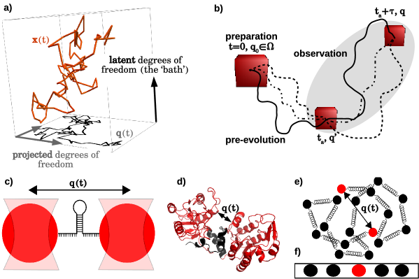
Figure 1: Schematics of projected observables, multi-point propagation and model systems. a) A physical observable corresponding to a simple lower-dimensional projection (shadow trajectory) of the full system’s trajectory (red line), defining projected and latent (hidden) degrees of freedom. b) Trajectories of length $t$ evolving from preparation, through an aging (or pre-evolution) period of length $t_{a}$, followed by the observation of duration $\tau=t-t_{a}$. c) Optical tweezers experimental set-up probing DNA-hairpin dynamics; d) Structure of the yeast PGK protein with the reduced coordinate represented by the arrow. e) Rouse model of a polymer chain, comprising Hookean springs with a zero rest-length immersed in a heat bath. The reduced coordinate corresponds to the end-to-end distance. f) Single file model with the tracer particle depicted in red.

For simplicity we use $\langle\cdot\rangle$ interchangeably to denote the average over an ensemble of trajectories at a given time and over time along a given trajectory, respectively, keeping in mind that they are identical only when the trajectory is much longer than the longest relaxation time $t_{\mathrm{rel}}$. The state of the observable is denoted by $q(t)\in\Xi$ (Fig. 1a, black trajectory), which we assume, without loss of generality, to be one dimensional (for the general case see the Appendix). Theoretically, each repetition of the experiment/process leads to an initial condition for $q(t)$ drawn randomly from the reduced stationary probability density $p_{\mathrm{inv}}(q_{0})$. In practice, however, this is not necessarily the case. For example, supercooled liquids [32, 33, 34] as well as polymeric [26, 27], spin [28, 29], and colloidal [30, 31] glasses are prepared by a quench in an external parameter (typically temperature) [26, 27, 28, 29, 30, 31], such that the observable $q(t)$ nominally attains a non-stationary initial condition. A process may also start with the observable internally constrained to a subdomain of $p_{\mathrm{inv}}(q_{0})$, e.g. a chaperone stabilizing a particular configuration of a folded protein, with the biological process starting upon unbinding of the chaperone [74]. In another example single-molecule enzyme experiments may monitor the statistics of substrate turnover, where $q(t)$ reflects the geometry of the catalytic site of an enzyme that is reactive only for a specific sub-ensemble of configurations [41, 42, 43]. Binding of a substrate molecule enforces an initial constraint on $q(t)$ thereby imposing non-stationary initial conditions on the chemical reaction. Alternatively, we may simply choose to initialize the experiment (i.e. reset our clock) a posteriori, such that $q(0)$ has a preset value, or we are dealing with a single, or a limited number of time-series [39] which do not sample $p_{\mathrm{inv}}(q_{0})$ sufficiently. In all these cases the observable is effectively not prepared in a stationary state, i.e. $p_{0}(q_{0})\neq p_{\mathrm{inv}}(q_{0})$.

The dynamics in aging systems is conventionally analyzed via the normalized two-time correlation function [28, 46, 47, 48, 45, 15]

$$C_{t_{a}}(\tau)=\frac{\langle q(\tau+t_{a})q(t_{a})\rangle-\langle q(\tau+t_{a})\rangle\langle q(t_{a})\rangle}{\langle q(t_{a})^{2}\rangle-\langle q(t_{a})\rangle^{2}}.$$ (1)

A system is often said to be aging if $C_{t_{a}}(\tau)$ strongly depends on $t_{a}$ in the sense that the relaxation of a system takes place on time-scales that grow with the age of the system $t_{a}$, and continue to do so beyond the largest times accessible within an experiment or simulation [21, 23, 24, 65, 25].

However, the analysis and interpretation of time-series of physical observables that show DTA require a fundamentally different approach irrespective of whether equilibrium is attainable in an experiment or not. We prove below that $C_{t_{a}}(\tau)$ cannot conclusively indicate whether time-translation invariance is broken (see Appendix C, Lemma 2); in particular it cannot disentangle broken time-translation invariance from “trivial” correlations with a non-stationary initial condition (i.e. from “weak” or “second order” non-stationarity [75]). This is particularly problematic if one uses Eq. (1) as a “definition of DTA” to infer whether a complex experimental system, such as an individual protein molecule [39, 38], evolves with broken time-translation invariance or not. Eq. (1) is nevertheless reasonable, albeit sub-optimal, for quantifying DTA in materials that are known to posses a broken time-translation invariance.

Our aim is to conclusively and unambiguously infer whether relaxation evolves with a broken time-translation invariance that is encoded in $G(q,t_{a}+\tau|q^{\prime},t_{a},q_{0}\!\in\!\Omega_{0})$, the probability density for the observable to be found in an infinitesimal volume element centered at $q$ at time $\tau+t_{a}$ given that it was at $q^{\prime}$ at time $t_{a}$ and started at $t=0$ somewhere in a subdomain $q_{0}\in\Omega_{0}\subset\Xi$ (Fig. 1b) with probability $p_{0}(q_{0})$. $\Omega_{0}$ is strictly non-empty and may be a point, an interval or a union of intervals.

The dynamics of an observable $q(t)$ is generally said to be time-translation invariant (mathematically referred to as “strictly stationary” [76, 75] or “well-aged” [77]) if the underlying (effective) equations of motion that govern the evolution of $q(t)$ do not explicitly depend on time. That is, the probability of a path $\{q(t)\}$ for $t\in[t_{a},t_{a}+\tau]$ does not depend on $t_{a}$. This is the case, e.g. in Newtonian dynamics or Langevin dynamics driven by Gaussian white noise [75] as well as generalized Langevin dynamics driven by stationary Gaussian colored noise [78, 79, 80]. Here $q(t)$ is said to be time-translation invariant if and only if (see also Definition 1 in Appendix C)

$$G(q,t_{a}+\tau|q^{\prime},t_{a},q_{0}\!\in\!\Omega_{0})=G(q,t^{\prime}+\tau|q^{\prime},t^{\prime},q_{0}\!\in\!\Omega_{0}),$$ (2)

holds for any $\tau$ and $t^{\prime}$ . Conversely, if time-translation invariance is broken we say that the system is dynamically time asymmetric. That is, time-translation invariance is broken if and only if the two-point conditioned Green’s function $G(q,t_{a}+\tau|q^{\prime},t_{a},q_{0}\!\in\!\Omega_{0})$ depends on $t_{a}$ (see also Definition 2 in Appendix C). The two-point conditioned Green’s function is defined as

$$G(q,t_{a}+\tau|q^{\prime},t_{a},q_{0}\!\in\!\Omega_{0})\equiv\frac{P(q,t_{a}+\tau,q^{\prime},t_{a},q_{0}\!\in\!\Omega_{0})}{P(q^{\prime},t_{a},q_{0}\!\in\!\Omega_{0})},$$ (3)

where $P(q,t_{a}+\tau,q^{\prime},t_{a},q_{0}\!\in\!\Omega_{0})$ denotes the joint density of $q(t)$ to be found initially within $\Omega_{0}$ and to pass $q^{\prime}$ at time $t_{a}$ and to end up in $q$ at time $t_{a}+\tau$, and $P(q^{\prime},t_{a},q_{0}\!\in\!\Omega_{0})$ the joint density of $q(t)$ to be found initially within $\Omega_{0}$ and to pass $q^{\prime}$ at time $t_{a}$.

Note that there seems to be some relation between DTA and aging. A system is typically said to be aging if $C_{t_{a}}(\tau)$ in Eq. (1) depends on $t_{a}$ (i.e. that $q(t)$ is weakly non-stationary) but in a specific manner, e.g. the so-called “slow”, non-stationary component of $C_{t_{a}}(\tau)$ must scale for all large $t_{a}$ as some power of $\tau/t_{a}$ [21, 23, 24] (for a rigorous discussion see [65]). However, this does not require that time-translation invariance (i.e. Eq. (2)) is broken [21, 23, 24]. So-called kinetically constrained models [25] and the spherical p-spin model [53, 52, 82], for example, have correlation functions Eq. (1) that show aging, but, when fully observed and not averaged over disorder (and only then), satisfy Eq. (2. Clearly, if time-translation invariance is broken (see also Definition 1 in the Appendix C) then $C_{t_{a}}(\tau)$ automatically depends on $t_{a}$. If the dynamics is furthermore such that $C_{t_{a}}(\tau)$ depends on $t_{a}$ as some power of $\tau/t_{a}$ (see Eq. (8) below as well as Eqs. (C7) and (C10) as well as [45, 83, 84]) and, in addition, equilibrium cannot be attained during an observation then DTA also implies aging dynamics. However, the converse is not true.

To connect the aging correlation function in Eq. (1) with Eq. (2) we note that the numerator in Eq. (1) involves averages

$$\langle q(t)\rangle\equiv\int_{\Xi}qG(q,t|q_{0}\!\in\!\Omega_{0})dq$$ (4)

$$\langle q(\tau+t_{a})q(t_{a})\rangle\equiv\!\!\int_{\Xi}\int_{\Xi}qq^{\prime}G(q,\tau+t_{a},q^{\prime},t_{a}|q_{0}\!\in\!\Omega_{0})dqdq^{\prime}$$

where the conditional density of the projected observable $G(q,t|q_{0}\!\in\!\Omega_{0})$ is discussed in [85, 19] and in Appendix B.2 (see Eq. (B2)). The three-point conditional probability density $G(q,\tau+t_{a},q^{\prime},t_{a}|q_{0}\!\in\!\Omega_{0})$ – the probability density for the observable to pass through an infinitesimal volume element centered at $q^{\prime}$ at time $t_{a}$ and end up in $q$ at time $\tau+t_{a}$ having started at $t=0$ in a subdomain $q_{0}\in\Omega_{0}\subset\Xi$ with probability $p_{0}(q_{0})$, is defined as (for details see Appendix B.2, Eq. (B20))

$$G(q,t_{a}+\tau,q^{\prime},t_{a}|q_{0}\!\in\!\Xi_{0})\equiv\frac{P(q,t_{a}+\tau,q^{\prime},t_{a},q_{0}\!\in\!\Omega_{0})}{P(q_{0}\!\in\!\Omega_{0})}.$$ (5)

Based on the mathematical properties of $G(q,t_{a}+\tau|q^{\prime},t_{a},q_{0}\!\in\!\Omega_{0})$ and $G(q,t_{a}+\tau,q^{\prime},t_{a}|q_{0}\!\in\!\Xi_{0})$ we prove in the Appendix C (see Theorem 1, Corollary 1.1 and, Lemma 2) that $C_{t_{a}}(\tau)$ in Eq. (1) can show a $t_{a}$-dependence even if Eq. (2) is satisfied, i.e. when the system is time-translation invariant. That is, if the system is dynamically time asymmetric then $C_{t_{a}}(\tau)$ depends on $t_{a}$, whereas the converse is not necessarily true. In turn this implies that one cannot determine on the basis of $C_{t_{a}}(\tau)$ derived from a time-series $q(t)$ whether time-translation invariance is broken, and a definitive and unambiguous indicator must be sought for.

We demonstrate this using the cleanest and most elementary example of a time-translation invariant system – a Brownian particle confined to a box of unit length (i.e. $L=1$) evolving from a a point $\Omega_{0}=x_{0}$ and from a uniform distribution within an interval $\Omega_{0}=[a,b]$ for some $0<a<b<1$. For this example the denominator in Eq. (3) is defined as $P(q^{\prime},t,q_{0}\!\in\!\Omega_{0})\equiv\int_{a}^{b}Q(q^{\prime},t|q_{0})dq_{0}$ and the numerator as $P(q,t_{a}+\tau,q^{\prime},t_{a},q_{0}\!\in\!\Omega_{0})\equiv Q(q,\tau+t_{a}|q^{\prime})P(q^{\prime},t_{a},q_{0}\!\in\!\Omega_{0})$, where $Q(x,t|x_{0})$ denotes the propagator of the confined Brownian particle. Plugging into Eq. (3) confirms the validity of Eq. (2) and hence time-translation invariance. Nevertheless, the very same system exhibits a $t_{a}$-dependence of the aging autocorrelation function defined in Eq. (1) over more than two orders of magnitude in time measured in units of the relaxation time $t_{\rm rel}=L^{2}/D\pi^{2}$ as depicted explicitly in Fig. 2. Note that by allowing the box to become macroscopic in size (i.e. $L\to\infty$) the relaxation time and thereby the extent of the $t_{a}$-dependence can become arbitrarily large when expressed in absolute units.

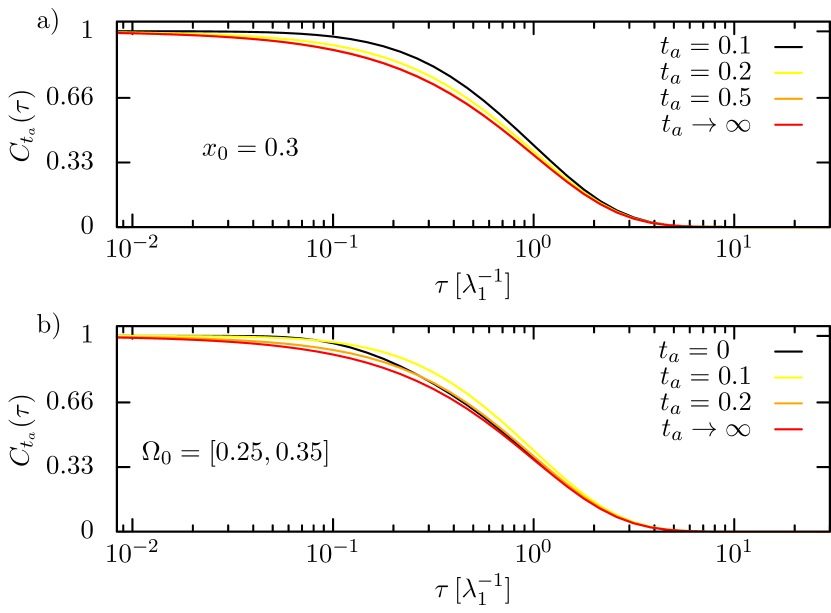
Figure 2: Aging correlation functions display fictitious dynamical time asymmetry in time-translation invariant systems. Analytical results for the aging correlation function $C_{t_{a}}(\tau)$ defined in Eq. (1) for a Brownian particle confined to a unit box evolving from a) the point $\Omega_{0}=0.3$ and b) the interval $\Omega_{0}=[0.25,0.35]$ for several values of the aging time $t_{a}$. Time $\tau$ is expressed in units of the relaxation time $\lambda_{1}^{-1}$.

A general mathematical analysis (see Appendix B.2) therefore necessarily ties DTA to the three-point (non-Markovian) conditional probability density, $G(q,\tau+t_{a},q^{\prime},t_{a}|q_{0}\in\Omega_{0})$. If the projected dynamics is Markovian it is in turn fully described by two-point conditional densities $G_{\mathrm{Markov}}(q,\tau+t_{a},q^{\prime},t_{a}|q_{0}\in\Omega_{0})=G(q,\tau|q^{\prime},0)G(q^{\prime},t_{a}|q_{0}\in\Omega_{0})$. If, on the other hand, the reduced dynamics is non-Markovian but the initial condition is sampled from the full (invariant) stationary density $p_{0}(q_{0})\to p_{\mathrm{inv}}(q_{0})$ (or equivalently, $\Omega_{0}=\Xi$), we have $G(q,\tau+t_{a},q^{\prime},t_{a}|q_{0}\in\Xi)=G(q,\tau|q^{\prime},0)p_{\mathrm{inv}}(q^{\prime})$. In both cases there is no DTA (see Appendix C). To quantify broken time-translation invariance on the level of reduced phase space probability densities we therefore define the time asymmetry index as

$$\Upsilon_{\Omega_{0}}(t_{a},\tau)\equiv\int_{\Omega}dq \int_{\Omega}dq^{\prime}\bigg{[}G(q,\tau+t_{a},q^{\prime},t_{a}|q_{0}\!\in\!\Omega_{0})\times$$

$$\ln\frac{G(q,\tau+t_{a},q^{\prime},t_{a}|q_{0}\!\in\!\Omega_{0})}{G(q,\tau|q^{\prime})G(q^{\prime},t_{a}|q_{0}\!\in\!\Omega_{0})}\bigg{]}$$ (6)

where for notational convenience we henceforth drop the explicit dependence on $\Omega_{0}$, i.e. $\Upsilon_{\Omega_{0}}(t_{a},\tau)\equiv\Upsilon(t_{a},\tau)$. The time asymmetry index measures the relative entropy between the actual evolution of the observable and a corresponding “fictitious” dynamics that has the same probability density of the intermediate point $q$ at time $t_{a}$ but where at time $t_{a}$ the latent degrees of freedom are instantaneously quenched to equilibrium. Broken time translation invariance reflects that the effective equations of motion that govern the evolution of $q(t)$ change in time as a result of the relaxation of the hidden DOF the observable is coupled to. That is, if one were e.g. to derive an effective generalized Langevin equation for $q(t)$ the latter would contain a memory kernel and noise that depend explicitly on the time elapsed since the preparation of the system (see e.g. [86]).

A broken time-translation invariance is evidently a clear signature of non-equilibrium dynamics and therefore intimately related to entropy production. $\Upsilon$ may thus also be given a thermodynamic interpretation as an entropy associated with the breaking of time-translation invariance in analogy to the “instantaneous excess free energy” – the relative entropy between $G(q,t|q_{0}\in\Omega_{0})$ and $p_{\mathrm{inv}}(q)$ [87, 88, 89, 19]. Therefore it appears that the entropy of breaking time-translation invariance measures the instantaneous thermodynamic displacement of latent degrees of freedom at time $t_{a}$ from their stationary state. Note that $\Upsilon(t_{a},\tau)>0$ also implies a violation of the fluctuation-dissipation theorem for non-Markovian system because it implies that the “bath” is non-stationary [90]. In general $\Upsilon$ is experimentally measurable simply by monitoring the time-series of the observable $q(t)$ (for details see Appendix D.4).

The relative entropy is a pseudo-metric and therefore the absolute value of the time asymmetry index (other than $\Upsilon(t_{a},\tau)=0$ implying time-translation invariance and $\Upsilon(t_{a},\tau)>0$ its violation) does not necessarily immediately allow for a quantitative comparison of DTA in different systems with disparate dimensionality. It is always meaningful when one considers a comparison of the same system and observable under different conditions (e.g. initial conditions, values of control parameters etc.). If one aims at comparing quantitatively DTA in different systems and/or observables one should instead consider a symmetrized version of the relative entropy (see e.g. [91]).

The time asymmetry index is constructed to detect and quantify conclusively broken time-translation invariance according to Eq. (2). It effectively measures the instantaneous relaxation of the latent degrees of freedom and is unaffected by spurious non-stationarity due to correlations between the value of the observable at time $t_{a}+\tau$ and the particular “initial” value at time $t_{a}$. These correlations are spurious because they exist for any $t_{a}$ and relax as a function of $\tau$ irrespective of whether a system is time-translation invariant or not.

By construction $\Upsilon(t_{a},\tau)\geq 0$ and is identically zero for any $t_{a}$ and $\tau$ if and only if $q(t)$ is time-translation invariant. In turn, the observable $q(t)$ is time-translation invariant if and only if it is Markovian and/or $q(t=0)$ is sampled from a distribution converging in law to the invariant measure (the proof is presented in the Appendix C, Theorem 2 and Corollary 1.1). As a result $\Upsilon(t_{a},\tau)$ is identically zero for all $\tau$ and $t_{a}$ for the time-translation invariant dynamics of a confined Brownian particle evolving from a non-equilibrium initial condition (see, however, the fictitious DTA due to weak non-stationarity that is implied by the aging autocorrelation function in Fig. 2). Moreover, the extent of DTA is limited by the relaxation time $t_{\mathrm{rel}}$ such that $\Upsilon(t_{a},\tau)\to 0$ whenever $t_{a}\gg t_{\mathrm{rel}}$ or $\tau\gg t_{\mathrm{rel}}$. Obviously, if the full system is initially quenched into any non-stationary initial condition (see e.g. [19]), then $\Upsilon(t_{a},\tau)>0$ as long as the projection renders the reduced dynamics non-Markovian. Therefore, as soon as $\Upsilon(t_{a},\tau)\neq 0$ for some values $t_{a}$ and $\tau$ smaller than $t_{\mathrm{rel}}$, the dynamics is time asymmetric, in specific cases with a self-similar scaling (see Appendix C, Propositions 1 & 2). In addition the following generic structure emerges:

$$C_{t_{a}}(\tau)=(1-\varphi)g_{1}(\tau)+\varphi g_{2}(\tau,t_{a}),$$ (7)

with $0<\varphi<1$ and $g_{1,2}$ depending on the details of the dynamics (see Appendix C, Theorem 3) in agreement with the properties of aging systems [46, 47, 48, 45, 49, 15, 28, 54]. These results are universal – they are independent of details of the dynamics, and, in particular, the underlying energy landscape.

Microscopically reversible dynamics in general allows for a spectral expansion of propagators and thus correlation and response functions (see e.g. Appendix B). Moreover, in specific cases the projection renders the observed dynamics self-similar with parameter $\alpha$, that is, a change of time-scale merely effects an $\alpha$-dependent renormalizion of the spectrum (for details see Definition 4 in the Appendix B.2). This arises, for example, when the observable corresponds to an internal distance within a single polymer molecule [92] (studied here in Figs. 3a and  4) or within individual protein molecules [93, 94], as well as in diffusion on fractal objects [95]. The aging correlation function in Eq. (1) then displays a power-law scaling for $\alpha>0$ (as in Fig. 3d and Eq. (C5) in the Appendix C) or, when $\alpha=0$ a logarithmic behavior (as observed in [38]; see also Eq. (C8) in the Appendix C). The latter is mathematically equivalent to the logarithmic relaxation found in [96]. For more details see Propositions 1 and 2 in the Appendix C, respectively. In particular for $\tau/t_{a}\gg 1$, in the glassy literature referred to as the “full aging” [49, 20, 97, 96] regime, we find (see Appendix C, Eqs. (C7) and (C10))

$$C_{t_{a}}(\tau)\simeq A+\begin{cases}B_{\alpha}\left(\frac{t_{a}}{\tau}\right)^{\alpha}&,\alpha>0,\\ B_{\alpha}\left(\frac{t_{a}}{\tau}\right)&,\alpha=0.\end{cases}$$ (8)

with constants $A$ and $B_{\alpha}$ that depend on the details of the dynamics. On a transient time-scale the asymptotic results in Eq. (8) agree with predictions of minimalistic “trap” models [21, 23, 24] as well as fractional dynamics and random walks with diverging waiting times [45, 98, 58] (for more details see also Remark 2.1 in the Appendix C). Fractional dynamics and random walks with long waiting times (that as well display DTA [83, 84, 98]) were in fact explicitly shown to arise as transients in projected dynamics when the latent degrees of freedom are orthogonal to $q(t)$ [85] and in the spatial coarse-graining of continuous dynamics on networks [99]. The phenomenology of systems displaying an algebraic scaling of $C_{t_{a}}(\tau)$ as in Eq. (8) is therefore by no means unique, and represents only a specific class of dynamical systems with a broken time-translation invariance. Dynamical time asymmetry is much more general.

Examples

It is not difficult to verify the above claims in practice as all corresponding quantities can readily be obtained from experimental or simulation-derived time-series. To that end we analyze DTA in four very different systems (see Fig. 1c-e): DNA hairpin dynamics measured by dual optical tweezers experiments, where $q(t)$ reflects the end-to-end distance (Fig. 1c and Appendix D.4.1) [68, 69], extensive MD simulations of internal motions of yeast PGK, where $q(t)$ corresponds to the inter-domain distance (Fig. 1d and Appendix D.4.2) [39], as well as two theoretical examples: the end-to-end distance fluctuations of a Rouse polymer chain [100] (Fig. 1e and Appendix D8) and tracer particle dynamics in a single file of impenetrable diffusing particles, where $q(t)$ reflects the position of the tracer particle [85, 101, 19] (Fig. 1f and Appendix D.3). The underlying energy landscapes of these four systems are fundamentally very different; the DNA-hairpin exhibits two well-defined metastable conformational states/ensembles [68, 69], the yeast PGK has a very rugged and apparently fractal energy landscape [39], that of the Rouse polymer is perfectly smooth and exactly parabolic, and that of the single file is flat with the tracer motion confined to a hyper-cone as a result of the non-crossing condition between particles. Yet, despite these striking differences, all systems display the same qualitative time asymmetric behavior, consistent with the proven universality of DTA.

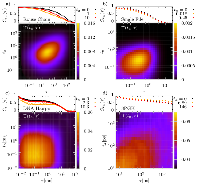
Figure 3: Aging two-point correlation function and time asymmetry index. $C_{t_{a}}(\tau)$ for different values of aging time $t_{a}$ and corresponding $\Upsilon(t_{a},\tau)$ for: a) the Rouse polymer chain with 50 beads with initial end-to-end distance in dimensionless units equal to $q_{0}=9.85$, which corresponds to the most likely end-to-end distance (the dimensionless relaxation time here corresponds to $t_{\mathrm{rel}}\simeq 253.38$); b) tracer-particle dynamics in a single file with $N=5$ confined to a box of unit length, tagging the central particle particle with initial condition $q_{0}=0.5$ (the relaxation time measured in natural units of the “collision time” of is $t_{\mathrm{rel}}\simeq 2.5$), c) the DNA-hairpin extension determined from a trajectory of length of $2.75\cdot 10^{4}$ ms sampled at $400\mathrm{kHz}$. The initial condition was taken at the absolute maximum of equilibrium probability density $q_{0}=2.0\pm 1$ nm, and $q$ refers to deviations from the mean distance $\langle d\rangle$, i.e. $q(t)=d(t)-\langle d\rangle$ (the relaxation time is $t_{\mathrm{rel}}\approx 15$ ms); The statistical error in determining $\Upsilon(t_{a},\tau)$ from the hairpin data is less than 1% (see Fig. D6 in the Appendix D.4.1); d) inter-domain motion between the centers of mass of the N-terminal (residues 1-185) and C-terminal domains (residues 200-389) in yeast PGK determined from a $200$ ns atomistic MD simulation sampled every $150$ ps. The initial condition was $q_{0}=0.01\pm 0.2$ nm relative to the average inter-domain distance $\langle d\rangle$, i.e. $q(t)=d(t)-\langle d\rangle$. c) was obtained from experimental data of Refs. [68, 69] and d) was determined from molecular dynamics simulations in Ref. [39]. Further details can be found in Appendix D. “Transient aging” in $C_{t_{a}}(\tau)$ arises whenever there is a region $(t_{a},\tau)$ where $\Upsilon(t_{a},\tau)>0$. In the case of PGK (panel d) $t_{\mathrm{rel}}$ is not reached within the simulation time, which renders the system virtually eternally time asymmetric and “forever aging” [39, 102].

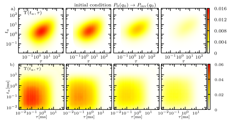
Figure 4: Attenuation and disappearance of dynamical time asymmetry upon approaching stationary initial conditions. Gradual vanishing of the time asymmetry index $\Upsilon(t_{a},\tau)$ when the initial distribution of the projected coordinate $p_{0}(q_{0})$ is sampled from a distribution being closer and closer to the density of the invariant measure, $p_{\mathrm{inv}}(q_{0})$ for: a) Rouse model of a polymer chain (the parameters are the same as in Fig. 3); The initial end-to-end distance is sampled from intervals (from left to right): $q_{0}=$9.85, $q_{0}\in[9-11]$, $q_{0}\in[7-13]$ and $q_{0}\in[4-16]$, respectively. b) experimental data for the DNA-hairpin. The initial conditions (relative to the mean value $\langle d\rangle$, that is, $d(t)=q(t)+\langle d\rangle$) are sampled (from left to right) from the following intervals: $q_{0}\in[1,3]$ nm, $q_{0}\in[-3,7]$ nm, $q_{0}\in[-6,10]$ and $q_{0}\in[-8,12]$ nm, respectively. When the initial condition is sampled from a distribution closer to the invariant measure, DTA vanishes confirming the claims of our theory.

The aging correlation functions $C_{t_{a}}(\tau)$ and time asymmetry indices $\Upsilon(t_{a},\tau)$ are shown in Fig. 3. With the exception of the PGK protein, which does not equilibrate within the duration of the trajectory, in agreement with previous findings [39], DTA is manifested as a transient phenomenon. The precise form of $C_{t_{a}}(\tau)$ depends on the details of the dynamics, which naturally vary between the systems. Moreover, the dependence of $C_{t_{a}}(\tau)$ on $t_{a}$ is non-monotonic. The generic form of $\Upsilon(t_{a},\tau)$ displays an initial increase towards a plateau, followed by a long-time decay to zero, which can be understood as follows. Irrespective of the details a finite time is required in order to allow for a build-up of memory, that is, of correlations between the instantaneous state of the projected observable and the initial condition of the latent variables. The memory at some point reaches a maximum. Afterwards, the memory of the preparation of the system is progressively lost as a result of the mixing of trajectories in full phase space during relaxation. Due to a relatively higher sampling frequency and sufficiently long sampling times that extend beyond the relaxation time all these effects are resolved in the experimental DNA-hairpin data but not in the case of the PGK simulation.

Moreover, a hallmark of aging is that at least part of the relaxation of a system takes place on time-scales that grow with the age of the system $t_{a}$, and continue to do so up to the largest times accessible within an experiment or simulation. Interestingly, Figs. 3 and 4 show that the relaxation time increases (at least transiently) with the aging time, i.e. $\Upsilon(t_{a},\tau)$ decays with $t$ more slowly as $t_{a}$ grows at least up to a threshold time. If an experiment or simulation does not reach this threshold time the breaking of time-translation invariance would seemingly take place on timescales that grow indefinitely, somewhat similar to the aging phenomenon. Note that the threshold time may become arbitrarily large in large systems (e.g. the relaxation time and thus the threshold time in natural units for the Rouse polymer and single file grow with the number of particles as $\propto N^{2}$ (see e.g. Fig. D2 in the Appendix D8); for any duration of an observation one may find a $N$ that makes DTA appear as everlasting).

One appreciates that $\Upsilon(t_{a},\tau)$ truly quantifies the degree of broken time-translation invariance and not correlations with the value of the observable at $t_{a}$. This is also the reason why $\Upsilon(t_{a},\tau)$ decays to zero on a time-scale shorter than $C_{t_{a}}(\tau)$. $C_{t_{a}}(\tau)$ starts at 1 and decays to zero as a result of “forgetting the initial condition”. Because the probability density of being found at a given point always depends trivially on $t_{a}\neq 0$ (see Eq. (5)) irrespective of whether time-translation invariance in Eq. (2) is broken or satisfied, $C_{t_{a}}(\tau)$ displays non-stationarity manifested in a $t_{a}$-dependence even for time-translation symmetric dynamics. Conversely, $\Upsilon(t_{a},\tau)$ is constructed to not be affected by such spurious non-stationarity. Instead, it reflects how far the latent degrees of freedom are displaced from equilibrium at time $t_{a}$. In other words, $\Upsilon(t_{a},\tau)$ compares the probability densities of the actual dynamics with those of fictitious dynamics that have the same probability density at time $t_{a}$ but in which at time $t_{a}$ the latent degrees of freedom are quenched to equilibrium (see Eq. (B25)).

One can look at $\Upsilon(t_{a},\tau)$ in two ways; as a function of $\tau$ at fixed $t_{a}$ and as a function of $t_{a}$ at fixed $\tau$. While the former intuitively reflects how the relaxation of the observable to equilibrium depends on the instantaneous (“initial”) state of the latent degrees of freedom at time $t_{a}$, the latter measures how the correlation of the value of the observable at two times separated by $\tau$ changes due to the relaxation of the latent degrees of freedom to equilibrium. The time asymmetry index therefore provides access to the dynamics of hidden degrees of freedom coupled to the observable through an analysis of time-series derived from measurements on the observable.

A verification that a breaking of time-translation invariance occurs whenever the distribution of initial conditions sampled by the experiment has not converged to the equilibrium distribution follows from inspection of $\Upsilon(t_{a},\tau)$ evolving from an ensemble of initial conditions being closer and closer to an equilibrium distribution, i.e. $\Omega_{0}\to\Xi$ (see Fig. 4 for the Rouse chain and DNA-hairpin). Indeed, $\Upsilon(t_{a},\tau)$ progressively vanishes when the initial condition becomes sampled from a distribution approaching the invariant measure, $p_{0}(q_{0})\to p_{\mathrm{inv}}(q_{0})$. In the Appendix C we prove that this is a general effect (Theorem 1), independent of any details of the dynamics.

Discussion

Non-stationary behavior of physical observables is traditionally considered as being important in systems with glassy, aging dynamics, such as polymer, spin or colloidal glasses, that attain glassy properties upon a quench in an external parameter [26, 27, 28, 29, 30, 31]. During, for example, a temperature quench, the system (e.g. a supercooled liquid or a set of spins) at some point cannot keep pace with rapid changes in the bath, and is pushed out of equilibrium [14]. After the quench at $t=0$ the observable is thus (at least weakly) non-stationary – it is sampled from and averaged over a non-equilibrium ensemble, i.e. $p_{0}(q_{0})\neq p_{\mathrm{inv}}(q_{0})$. The absence of such an obvious quench rendered the origin of non-stationary, apparent aging behavior in biological macromolecules somewhat mysterious [36, 37, 39, 40, 41, 42, 43]. However, in biological systems the observable can become quenched implicitly, e.g. by the ’locking in’ of a protein’s configuration by a chaperone [74], the configurational requirements for enzymatic catalysis [41, 42, 43], or simply by the under-sampling of equilibrium such as in single-molecule experiments and particle-based computer simulations [39], such that $p_{0}(q_{0})\neq p_{\mathrm{inv}}(q_{0})$. In an experiment one can check for non-stationarity of initial conditions, e.g. by inspecting whether histograms of the observable (also referred to as the “occupation time fraction” or “empirical density”) at $t=0$ and at all later times coincide [103].

Here, we highlight a more general and wide-spread aspect of out-of-equilibrium dynamics of physical observables – dynamical time asymmetry. The requirements for DTA to occur are much weaker than for aging, and it is manifested in a very broad variety of experimental situations, and in particular, one may also expect aging physical observables probed in many experiments to display DTA. Even measurements on polymer, spin and colloidal glasses have built-in underlying projections. For example, in tensile creep experiments in polymeric glasses the motion in a (cold) polymer is projected onto a local, effectively one-dimensional flow [26]. In supercooled liquids and colloidal glasses the dynamics is typically projected onto local particle displacements, pair correlation functions and structure factors [33, 34, 30, 31]. In bulk experiments with spin glasses and supercooled liquids one measures quantities such as the average single-spin auto-correlation function [21, 104] , magnetization, conductance or the dielectric constant, which correspond to projections of many-particle dynamics onto a scalar parameter [29, 32, 49]. In biological macromolecules the projection may correspond to [37, 39] or depend on [41, 42, 43] some internal distance within the macromolecule. These projections lead to non-Markovian observables evolving from non-stationary initial conditions which are in turn expected to show DTA. In fact we can appreciate that the physical origin of DTA in both, ’traditional’ glassy systems [26, 27, 28, 29, 30, 31] and biological matter [36, 37, 39, 40, 41, 42, 43], is qualitatively the same and simply results from non-stationary initial conditions of non-Markovian observables (see Observation 2 in the Appendix C). In most of these aforementioned systems the dynamics is also aging [26, 27, 28, 29, 30, 31, 36, 37, 39].

It is important to realize that it is not possible to infer from a finite measurement whether the observed process is genuinely non-ergodic (i.e. a result of some true localization phenomenon in phase space) or whether the observation is made on an ergodic system but on a time-scale shorter the relaxation time [85] (note that a comparison of the dynamics of PGK in Fig. 3d with a transient shorter than the relaxation time in any of the remaining examples in Fig. 3a-c shows no qualitative difference). A theoretical description of both scenarios on time-scales shorter than the relaxation time is in fact identical (for details see [85] as well as [24] in the context of glasses).

Although sporting characteristics commonly associated with aging, DTA and aging are not quite the same thing. DTA does not require the relaxation to take place on time-scales that grow indefinitely with the age of the system $t_{a}$ beyond the largest times accessible within an experiment or simulation, nor does it impose requirements on the precise form of the dependence on $t_{a}$. It is likely to be a ubiquitous phenomenon that is frequently observed in measurements of projected observables. In turn, aging does not imply a broken time-translation invariance according to Eq. (2).

Note, however, that many paradigmatic models of aging dynamics (e.g. continuous-time random walks with diverging mean waiting times and fractional diffusion [83, 84, 45]) display a (strongly) broken time-translation invariance. Furthermore, most experimental observations of aging dynamics monitor projected observables, e.g. magnetization, single-spin auto-correlation functions averaged over the sample and potentially also over disorder [26, 27, 28, 29, 30, 31, 36, 37, 39]. The dynamics of these observables is thus almost surely non-Markovian [85] and expected to display DTA.

The observation of $\Upsilon(t_{a},\tau)>0$ on a given scale of $t_{a}$ and $\tau$ implies that the dynamics of the observable $q(t)$ fundamentally changes in the course of time as a results of the relaxation of hidden DOF, and does not reflect correlations with the value of the observable at zero time $q(0)$. That is, the effective equations of motion for $q(t)$ truly change in time. In biological systems and in particular enzymes and other protein nanomachines non-stationary effects are thought to influence function, e.g. memory effects in catalysis [41, 42, 43]. This is particularly important because some larger proteins potentially never relax within their life-times, i.e. before they become degraded (note that relaxation corresponds to attaining the spontaneous unfolding-refolding equilibrium). This renders the dynamically time asymmetric regime virtually ’forever lasting’ and implies that the system is aging [39]. As proteins are produced in the cell in an ensemble of folded configurations under the surveillance of chaperones [74], our theory implies that DTA during function [41, 42, 43] should arise naturally and generically due to the memory of a protein’s preparation.

We expect DTA to be particularly pronounced in measurements on systems with entropy-dominated, temporally heterogeneous collective conformational dynamics involving (transient) local structure-formation where the background DOF evolve on the same time-scale as the observable [38], and we suggest the breaking of time-translation invariance to be closely related to the phenomenological notion of “dynamical disorder” in biomolecular dynamics [41, 42, 43, 71].

Our results have some intriguing implications. First, a quench in an external parameter and the mere under-sampling of equilibrium distributions give rise to qualitatively equivalent manifestations (but potentially with a largely different magnitude and duration) of DTA as soon as the observable follows a non-Markovian evolution (see Appendix C, Observation 2). This has important practical consequences in fields such as single-molecule spectroscopy and computer simulations of soft and biological matter, which often suffer from sampling constraints. Second, broken time-translation invariance is ’in the eye of the beholder’, insofar as its degree depends on the specific observable; there should exist a (potentially less) reduced coordinate, not necessarily accessible to experiment (e.g. when we follow all degrees of freedom), according to which the same system will exhibit virtually time-translation invariant dynamics. However, auto-correlation functions will show a $t_{a}$-dependence for essentially any non-stationary initial condition in any system.

A broken time-translation invariance was shown to be linked to a form of entropy embodied in a time asymmetry index that is a measure of the instantaneous thermodynamic displacement of latent, hidden degrees of freedom from their stationary state. The time asymmetry index may therefore be used to probe systematically the time-scale of dynamics of hidden, slowly relaxing degrees of freedom relative to the time-scale of the evolution of the observable. In particular, it may be useful as a practical tool to discriminate between situations where the hidden degrees of freedom evolve through a sequence of local equilibria that would yield small values of the time asymmetry index $\Upsilon$ from those cases where their evolution is transient and slow on the time-scale of the observable thus implying a significant $\Upsilon$. For example, $\Upsilon$ may potentially provide additional insight into the dominant folding mechanism of a protein from single-molecule force-spectroscopy data [105], in particular about the much debated heterogeneity of folding trajectories and its functional relevance [106, 107].

The present theory ties dynamical time asymmetry in a general setting to both the non-stationary preparation of an observable and its non-Markovian time evolution. Thereby it connects aspects of the better known phenomenology of aging of projected observables with the broken time-translation invariance observed in recent measurements on in soft and biological materials on a common footing. Moreover, dynamical time asymmetry is suggested to be a ubiquitous phenomenon in biological and materials systems.

APPENDIX

In this Appendix we present the main theorems needed for the article with the corresponding proofs. We treat the problem in a general setting, that is, not assuming that the full system is initially prepared in equilibrium. Further included are analytical results with details of calculations for the Rouse polymer and single file diffusion, all details of the numerical analyses of the DNA-hairpin and protein PGK data and further supporting results.

Contents

1. A Definitions, notation and preliminaries
2. B Dynamics of the projected lower-dimensional observable
   1. B.1 Spectral theory of projected dynamics
   2. B.2 Three-point dynamics and breaking of time-translation invariance
3. C Main theorems with proofs
4. D Physical models, experimental and simulation data
   1. D.1 Fictitious dynamical time asymmetry in a time-translation invariant system: the Brownian particle in a box
   2. D.2 Rouse polymer model
   3. D.3 Single file diffusion
   4. D.4 Analysis of experimental and simulation data
      1. D.4.1 DNA-hairpin
      2. D.4.2 Yeast 3-phosphoglycerate kinase (PGK)

Appendix A Definitions, notation and preliminaries

We consider a stable conservative mechanical system in a continuous domain $\Omega\in\mathbb{R}^{d}$ that is at least weakly coupled to a thermal bath with Gaussian statistics with the longest correlation time $\tau_{b}$ being much shorter than that of the system, $\tau_{s}$ (i.e. $\tau_{b}\ll\tau_{s}$) such that the bath can be considered as representing stationary white noise on the time-scale of the system’s dynamics [73]. The thermal bath is either external or the result of integrating out an additional subset of internal degrees of freedom that relaxes much faster than the system. At any time $t$ the state of the system is specified by a $d$-dimensional state (column) vector $\mathbf{x}_{t}\in\mathbb{R}^{d}$, whose entries are generalized coordinates $x_{t,i}$. Note that the dynamics in soft matter and biological systems is typically strongly overdamped which we also assume here. The extension to underdamped systems is conceptually straightforward (since we consider microscopically reversible dynamics) [108], but since a broken time-translation invariance in soft and biological matter is not tied to momenta, we omit these for convenience. We are strictly interested in the evolution of $\mathbf{x}_{t}$ for $t\gg\tau_{b}$. It is well known that under certain technical conditions imposed on the dynamics of the bath [73], which we will not further detail here but are strictly granted for the physical systems relevant to the discussion, $\mathbf{x}_{t}$ evolves according to the It$\mathrm{\hat{o}}$ equation

$$d\mathbf{x}_{t}=\mathbf{F}(\mathbf{x}_{t})dt+\boldsymbol{\sigma}d\mathbf{W}_{t}$$ (A1)

where $\mathbf{W}_{t}$ is a $d$-dimensional vector of independent Wiener processes whose increments have a Gaussian distribution with zero mean and variance $dt$, i.e. $\mathbb{E}[dW_{t,i}dW_{t^{\prime},j}]=\delta_{ij}\delta(t-t^{\prime})dt$, $\mathbb{E}[\cdot]$ denotes the expectation over the ensemble of Wiener increments and where $\boldsymbol{\sigma}$ is a $d\times d$ symmetric noise matrix. If momentum coordinates were included $\boldsymbol{\sigma}$ would be positive semi-definite with zeros in the sector of position variables and non-zero terms proportional to the friction constant $\gamma$ in the momentum sector, and is strictly positive definite with terms $\propto\gamma^{-1}$ for over-damped dynamics (i.e. for $\gamma\gg 1$) [108]). We focus on microscopically reversible dynamics, that is, we consider $d$-dimensional Markovian diffusion with a $d\times d$ symmetric positive-definite diffusion matrix $\mathbf{D}=\boldsymbol{\sigma}\boldsymbol{\sigma}^{T}/2$ and mobility tensor $\mathbf{M}=\mathbf{D}/k_{\mathrm{B}}T$ (with $\beta^{-1}\equiv k_{\mathrm{B}}T$ being the thermal energy) in a drift field $\mathbf{F}(\mathbf{x})$, such that $\mathbf{M}^{-1}\mathbf{F}(\mathbf{x})=-\nabla\varphi(\mathbf{x})$ is a gradient flow. The drift field $\mathbf{F}(\mathbf{x}):\mathbb{R}^{d}\to\mathbb{R}^{d}$, is either nominally confining (in this case $\Omega$ is open) or is accompanied by corresponding reflecting boundary conditions at $\partial\Omega$ (in this case $\Omega$ is closed) thus guaranteeing the existence of an invariant measure and hence ergodicity [73, 108].

On the level of probability measures in phase space the dynamics is governed by the (forward) Fokker-Planck operator $\hat{\mathcal{L}}:V\to V$, where $V$ is a complete normed linear vector space with elements $f\in C^{2}(\mathbb{R}^{d})$. In particular,

$$\hat{\mathcal{L}}=\nabla\cdot\mathbf{D}\nabla-\nabla\cdot\mathbf{F}(\mathbf{x}).$$ (A2)

$\mathbf{F}(\mathbf{x})$ is assumed to be sufficiently confining, i.e. $\lim_{\mathbf{x}\to\infty}P(\mathbf{x},t)=0,\forall t$ sufficiently fast to assure that $\hat{\mathcal{L}}$ corresponds to a coercive and densely defined operator on $V$ with a pure point spectrum [109, 110, 111]. $\hat{\mathcal{L}}$ propagates probability measures $\mu_{t}(\mathbf{x})$ in time, which will throughout be assumed to possess well-behaved probability density functions $P(\mathbf{x},t)$, i.e. $d\mu_{t}(\mathbf{x})=P(\mathbf{x},t)d\mathbf{x}$. The nullspace of $\hat{\mathcal{L}}$ (i.e. the solution of $\hat{\mathcal{L}}P_{\mathrm{eq}}(\mathbf{x})=0$) is the equilibrium (Maxwell-)Boltzmann-Gibbs distribution, $P_{\mathrm{eq}}(\mathbf{x})=Q^{-1}\mathrm{e}^{-\beta\varphi(\mathbf{x})}$, with partition function $Q=\int_{\Omega}d\mathbf{x}\mathrm{e}^{-\beta\varphi(\mathbf{x})}$. We define the (forward) propagator $\hat{U}(t)=\mathrm{e}^{\hat{\mathcal{L}}t}$ that is the generator of a semi-group $\hat{U}(t+t^{\prime})=\hat{U}(t)\hat{U}(t^{\prime})$. The formal solution of the Fokker-Planck equation $(\partial_{t}-\hat{\mathcal{L}})P(\mathbf{x},t)=0$ is thereby given as $P(\mathbf{x},t)=\hat{U}(t)P(\mathbf{x},0)$. The expectation over the ensemble of paths $\mathbf{x}_{t}$ will be denoted by $\langle\cdot\rangle$ and in the case of a physical observable $\mathcal{B}(\mathbf{x}_{t})$ is given by

$$\langle\mathcal{B}(\mathbf{x}_{t})\rangle\equiv\int\mathcal{B}(\mathbf{x})d\mu_{t}(\mathbf{x})\equiv\int_{\Omega}\mathcal{B}(\mathbf{x})P(\mathbf{x},t)d\mathbf{x}\equiv\int_{\Omega}\mathcal{B}(\mathbf{x})\hat{U}(t)P(\mathbf{x},0)d\mathbf{x}$$ (A3)

Part of the analysis will involve the use of spectral theory in Hilbert space, for which it is convenient to introduce the bra-ket notation; the ’ket’ $|g\rangle$ represents a vector in $V$ written in position basis as $g(\mathbf{x})\equiv\langle\mathbf{x}|g\rangle$, and the ’bra’ $\langle h|$ as the integral $\int d\mathbf{x}h^{\dagger}(\mathbf{x})$. The scalar product is defined with the Lebesgue integral $\langle h|g\rangle=\int d\mathbf{x}h^{\dagger}(\mathbf{x})g(\mathbf{x})$. In this notation we have the following evolution equation for the probability density function starting from an initial condition $|p_{0}\rangle$: $|p_{t}\rangle=\mathrm{e}^{\hat{\mathcal{L}}t}|p_{0}\rangle$. Since the process is ergodic we have $\lim_{t\to\infty}\mathrm{e}^{\hat{\mathcal{L}}t}|p_{0}\rangle=|\mathrm{eq}\rangle$, where $\langle\mathbf{x}|\mathrm{eq}\rangle=P_{\mathrm{eq}}(\mathbf{x})$. We also define the (typically non-normalizable) ’flat’ state $|\text{--}\rangle$, such that $\langle\mathbf{x}|\text{--}\rangle=1$ and $\langle\text{--}|p_{t}\rangle=1$. Hence, $\partial_{t}\langle\text{--}|p_{t}\rangle=0$ and $\langle\text{--}|\hat{\mathcal{L}}=0$.

Whereas $\hat{\mathcal{L}}$ by itself is not self-adjoint, it is orthogonally equivalent to a self-adjoint operator, i.e. the operator $\hat{\mathcal{L}}_{s}=\mathrm{e}^{\beta\varphi(\mathbf{x})/2}\hat{\mathcal{L}}\mathrm{e}^{-\beta\varphi(\mathbf{x})/2}$ is self-adjoint, and, moreover the operator $\mathrm{e}^{\beta\varphi(\mathbf{x})}\hat{\mathcal{L}}$ is self-adjoint (for a proof see [108]). Because any self-adjoint operator in Hilbert space is diagonalizable, $\hat{\mathcal{L}}$ is diagonalizable as well, but with a separate set of left and right bi-orthonormal eigenvectors $\langle\psi^{L}_{k}|$ and $|\psi^{R}_{k}\rangle$, respectively. That is, $\hat{\mathcal{L}}|\psi^{R}_{k}\rangle=-\lambda_{k}|\psi^{R}_{k}\rangle$ and $\langle\psi^{L}_{k}|\hat{\mathcal{L}}=-\lambda_{k}\langle\psi^{L}_{k}|$ with real eigenvalues $\lambda_{k}\geq 0$ (assured by detailed balance) and where $\lambda_{0}=0$, $|\psi^{R}_{0}\rangle=|\mathrm{eq}\rangle$, $\langle\psi^{L}_{0}|=\langle\text{--}|$, and $\langle\psi^{L}_{k}|\psi^{R}_{l}\rangle=\delta_{kl}$. Moreover, since $\mathrm{e}^{\beta\varphi(\mathbf{x})}\hat{\mathcal{L}}$ is self-adjoint it follows that that $|\psi^{L}_{k}\rangle=\mathrm{e}^{\beta\varphi(\mathbf{x})}|\psi^{R}_{k}\rangle$. The resolution of identity is given by $\mathbf{1}=\sum_{k}|\psi^{R}_{k}\rangle\langle\psi^{L}_{k}|$ and the propagator by $\hat{U}(t)=\sum_{k}|\psi^{R}_{k}\rangle\langle\psi^{L}_{k}|\mathrm{e}^{-\lambda_{k}t}$.

The Markovian Green’s function of the process $\mathbf{x}_{t}$ corresponds to the conditional probability density function for a localized initial condition $\langle\mathbf{x}|p_{0}\rangle=\delta(\mathbf{x}-\mathbf{x}_{0})$ and is defined as $Q(\mathbf{x},t|\mathbf{x}_{0},0)=\langle\mathbf{x}|\hat{U}(t)|\mathbf{x}_{0}\rangle$, such that the probability density starting from a general initial condition $|p_{0}\rangle$ becomes $P(\mathbf{x},t,p_{0})=\langle\mathbf{x}|\hat{U}(t)|p_{0}\rangle\equiv\int d\mathbf{x}_{0}p_{0}(\mathbf{x}_{0})Q(\mathbf{x},t|\mathbf{x}_{0},0)$. In the spectral representation the Green’s function reads

$$Q(\mathbf{x},t|\mathbf{x}_{0},0)=\sum_{k}\psi^{R}_{k}(\mathbf{x})\psi_{k}^{L}(\mathbf{x}_{0})\mathrm{e}^{-\lambda_{k}t},$$ (A4)

where the semi-group property means that $Q(\mathbf{x},\tau|\mathbf{x}_{0},0)=Q(\mathbf{x},t+\tau|\mathbf{x}_{0},t)$ is independent of $t$ as is easily verified via

$$\int_{\Omega}d\mathbf{x}^{\prime}Q(\mathbf{x},t|\mathbf{x}^{\prime},t^{\prime})Q(\mathbf{x}^{\prime},t^{\prime}|\mathbf{x}_{0},0)=\sum_{k,l}\psi^{R}_{k}(\mathbf{x})\langle\psi^{L}_{k}|\psi^{R}_{l}\rangle\psi^{L}_{l}(\mathbf{x}_{0})\mathrm{e}^{-\lambda_{k}(t-t^{\prime})-\lambda_{l}t^{\prime}}\equiv Q(\mathbf{x},t|\mathbf{x}_{0},0),$$ (A5)

where we have used that $\langle\psi^{L}_{k}|\psi^{R}_{l}\rangle=\delta_{k,l}$.

In the presence of a time-scale separation giving rise to local equilibrium the system’s dynamics may be coarse-grained further into a discrete-state Markov jump master equation (see e.g. [112, 113]). In this case the configuration space would be discrete and $d-$dimensional, $\hat{\mathcal{L}}$ would be replaced by a $d\times d$ symmetric stochastic matrix $\mathbf{M}$, and the Fokker-Planck equation by the master equation $\frac{d}{dt}Q=\mathbf{M}Q$. Since this situation corresponds to an approximate, lower-resolution dynamics of the system that is mathematically simpler and the mapping between the Fokker-Planck equation and Markov-state jump dynamics is well-known [112, 108, 103] and does not introduce any further conceptual changes (the complete spectral-theoretic approach in particular remains unchanged), we will without any loss of generality focus on the continuous scenario.

Appendix B Dynamics of the projected lower-dimensional observable

In order to describe the dynamics of the $r$-dimensional projected observable $\mathbf{q}=\boldsymbol{\Gamma}(\mathbf{x}):\mathbb{R}^{d}\to\mathbb{R}^{r}$ with $r<d$ and $\mathbf{q}$ lying in some orthogonal system in Euclidean space $\mathbf{q}\in\Xi(\mathbb{R}^{r})\subset\Omega(\mathbb{R}^{d})$, we define the operator $\hat{\mathcal{P}}_{\mathbf{x}}(\boldsymbol{\Gamma};\mathbf{q})$, such that, when applied to some function $Z(\mathbf{x})\in V$, $\hat{\mathcal{P}}_{\mathbf{x}}(\boldsymbol{\Gamma};\mathbf{q})$ gives (see [85])

$$\hat{\mathcal{P}}_{\mathbf{x}}(\boldsymbol{\Gamma};\mathbf{q})Z(\mathbf{x})\equiv\int_{\Omega}d\mathbf{x}\delta(\boldsymbol{\Gamma}(\mathbf{x})-\mathbf{q})Z(\mathbf{x}),$$ (B1)

where $\delta(\mathbf{y})$ is to be understood in the distributional sense. We can now define the (in general) non-Markovian two-point conditional probability density of projected dynamics starting from $\mathbf{q}_{0}\in\Xi_{0}$, where the subdomain $\Xi_{0}$ is not necessarily simply connected, with the extended operator $\hat{\mathcal{P}}_{\mathbf{x}}(\boldsymbol{\Gamma};\mathbf{q}\in\Xi_{0})=\int_{\Xi_{0}}d\mathbf{q}\hat{\mathcal{P}}_{\mathbf{x}}(\boldsymbol{\Gamma};\mathbf{q})$ in terms of the single-point and joint two-point density $P_{p_{0}}^{0}(\mathbf{q}_{0}\in\Xi_{0})$ and $P_{p_{0}}(\mathbf{q},t,\mathbf{q}_{0}\in\Xi_{0})$, respectively, as

$$G_{p_{0}}(\mathbf{q},t|\mathbf{q}_{0}\in\Xi_{0})=\frac{P_{p_{0}}(\mathbf{q},t,\mathbf{q}_{0}\in\Xi_{0})}{P_{p_{0}}^{0}(\mathbf{q}_{0}\in\Xi_{0})}\equiv\frac{\hat{\mathcal{P}}_{\mathbf{x}}(\Gamma;\mathbf{q})\hat{\mathcal{P}}_{\mathbf{x}_{0}}(\boldsymbol{\Gamma};\mathbf{q}_{0}\in\Xi_{0})Q(\mathbf{x},t|\mathbf{x}_{0},0)p_{0}(\mathbf{x}_{0})}{\hat{\mathcal{P}}_{\mathbf{x}_{0}}(\boldsymbol{\Gamma};\mathbf{q}_{0}\in\Xi_{0})p_{0}(\mathbf{x}_{0})}$$ (B2)

with the convention that $P_{p_{0}}(\mathbf{q},t,\mathbf{q}_{0})$ and $G_{p_{0}}(\mathbf{q},t|\mathbf{q}_{0})$ stand for $\Xi_{0}$ corresponding to a single point $\mathbf{q}_{0}$. The full system is said to have a stationary preparation if and only if $p_{0}(\mathbf{x}_{0})=P_{\mathrm{eq}}(\mathbf{x})$, whereas the projected observable is said to have a stationary preparation if and only if $\Xi_{0}=\Xi$. Note that $\lim_{t\to\infty}P_{p_{0}}(\mathbf{q},t,\mathbf{q}_{0}\in\Xi_{0})=P_{\mathrm{eq}}(\mathbf{q})\int_{\Xi_{0}}d\mathbf{q}_{0}P_{p_{0}}(\mathbf{q}_{0})$, where we have defined $P_{\mathrm{eq}}(\mathbf{q})\equiv\hat{\mathcal{P}}_{\mathbf{x}}(\Gamma;\mathbf{q})P_{\mathrm{eq}}(\mathbf{x})$ as well as $P_{p_{0}}(\mathbf{q}_{0})\equiv\hat{\mathcal{P}}_{\mathbf{x}_{0}}(\boldsymbol{\Gamma};\mathbf{q}_{0})p_{0}(\mathbf{x}_{0})$. In turn it follows that $\lim_{t\to\infty}G_{p_{0}}(\mathbf{q},t|\mathbf{q}_{0}\in\Xi_{0})=P_{\mathrm{eq}}(\mathbf{q})$. Eq. (B2) demonstrates that the entire time evolution of projected dynamics starting from a fixed condition $\mathbf{q}_{0}$ depends on the initial preparation of the full system $p_{0}(\mathbf{x}_{0})$ as denoted by the subscript, which is the first signature of the non-stationary nature of projected dynamics. In addition, the dynamics described by Eq. (B2) is, except for quite exotic projections $\boldsymbol{\Gamma}(\mathbf{x})$, non-Markovian (see [85]).
We can now define averages and two-point correlation functions of $\mathbf{q}(t)$. The $n$-th moment of the position averaged over an ensemble of all projected non-Markovian evolutions prepared in the point $\mathbf{q}_{0}$ while the full system at $t=0$ is prepared in the state $p_{0}(\mathbf{x}_{0})$ is given by

$$\langle\mathbf{q}(t)^{n}\rangle^{\Xi_{0}}_{p_{0}}\equiv\int_{\Xi}d\mathbf{q}\mathbf{q}^{n}G_{p_{0}}(\mathbf{q},t|\mathbf{q}_{0}\in\Xi_{0}),\quad\langle\mathbf{q}^{n}\rangle^{\Xi_{0}}_{p_{0}}\equiv\int_{\Xi_{0}}d\mathbf{q}_{0}\mathbf{q}_{0}^{n}P_{p_{0}}(\mathbf{q}_{0})$$ (B3)

where we are here only interested in $n=1,2$, whereas the most general tensorial two-point $(0,t)$ (non-aging) correlation (i.e. covariance) matrix is defined as

$$\mathbf{C}_{\Xi_{0}}(t;p_{0})\! \equiv \!\langle\mathbf{q}(t)\otimes\mathbf{q}(0)\rangle^{\Xi_{0}}_{p_{0}}-\langle\mathbf{q}(t)\rangle_{p_{0}}^{\Xi_{0}}\otimes\langle\mathbf{q}\rangle^{\Xi_{0}}_{p_{0}}$$ (B4)

$$= \!\!\int_{\Xi}\!d\mathbf{q}\!\int_{\Xi_{0}}\!d\mathbf{q}_{0}(\mathbf{q}\otimes\mathbf{q}_{0})P_{p_{0}}(\mathbf{q},t,\mathbf{q}_{0})-\langle\mathbf{q}(t)\rangle^{\Xi_{0}}_{p_{0}}\otimes\langle\mathbf{q}\rangle^{\Xi_{0}}_{p_{0}},$$

such that $\lim_{t\to\infty}\mathbf{C}(t;p_{0})=0,\forall p_{0}$, where from the scalar version is in turn obtained by taking the trace

$$C_{\Xi_{0}}(t;p_{0})\equiv\langle\mathbf{q}(t)\cdot\mathbf{q}(0)\rangle^{\Xi_{0}}_{p_{0}}-\langle\mathbf{q}(t)\rangle_{p_{0}}^{\Xi_{0}}\cdot\langle\mathbf{q}\rangle^{\Xi_{0}}_{p_{0}}=\mathrm{Tr}\mathbf{C}_{\Xi_{0}}(t;p_{0})$$ (B5)

with the convention $\mathbf{C}_{\Xi_{0}}(t;P_{\mathrm{eq}})=\langle\mathbf{q}(t)\cdot\mathbf{q}(0)\rangle^{\Xi_{0}}_{\mathrm{eq}}-\langle\mathbf{q}(t)\rangle_{\mathrm{eq}}^{\Xi_{0}}\cdot\langle\mathbf{q}\rangle^{\Xi_{0}}_{\mathrm{eq}}\equiv\mathbf{C}_{\Xi_{0}}(t)$. We can equivalently define the time-dependent variance of $\mathbf{q}(t)$ with $\mathbf{q}(0)=\mathbf{q}_{0}\in\Xi_{0}$ as

$$\sigma_{\Xi_{0}}^{2}(t;p_{0})\equiv\langle\mathbf{q}(t)^{2}\rangle^{\Xi_{0}}_{p_{0}}-(\langle\mathbf{q}(t)\rangle_{p_{0}}^{\Xi_{0}})^{2}$$ (B6)

B.1 Spectral theory of projected dynamics

We now use spectral theory of the Markovian Green’s function in Eq. (A4) to analyze the general properties of the non-Markovian time evolution of the projected lower-dimensional observable $\mathbf{q}(t)$. As the initial preparation of the full system $p_{0}(\mathbf{x}_{0})$ was found to determine the point-to-point propagation of the probability density of $\mathbf{q}$, we begin by expanding the initial condition of the full system $p_{0}(\mathbf{x}_{0})$ in the eigenbasis of $\hat{\mathcal{L}}$, i.e. $p_{0}(\mathbf{x}_{0})=\sum_{l}|\psi_{l}^{R}\rangle\left\langle\psi_{l}^{L}|p_{0}\right\rangle$. The only assumptions made for $p_{0}(\mathbf{x}_{0})$ are that it is normalized, Lebesgue integrable (such that $\left\langle\psi_{l}^{L}|p_{0}\right\rangle$ exists) and locally sufficiently compact to assure that the projection at time $t=0$ does not project onto an empty set of the observable $\mathbf{q}_{0}$. By further introducing the elements of the following infinite-dimensional matrices

$$\Psi_{kl}(\mathbf{q})=\langle\psi^{L}_{k}|\delta(\boldsymbol{\Gamma}(\mathbf{x})-\mathbf{q})|\psi^{R}_{l}\rangle,\quad\Psi_{kl}(\Xi_{0})=\int_{\Xi_{0}}d\mathbf{q}\langle\psi^{L}_{k}|\delta(\boldsymbol{\Gamma}(\mathbf{x})-\mathbf{q})|\psi^{R}_{l}\rangle$$ (B7)

where $\lim_{\Xi_{0}\to\mathbf{q}}\Psi_{kl}(\Xi_{0})=\Psi_{kl}(\mathbf{q})$, we can express $P_{p_{0}}(\mathbf{q},t|\mathbf{q}_{0}\in\Xi_{0})$ in Eq. (B2) as

$$P_{p_{0}}(\mathbf{q},t,\mathbf{q}_{0}\in\Xi_{0})=\sum_{k}\mathrm{e}^{-\lambda_{k}t}\Psi_{0k}(\mathbf{q})\sum_{l}\Psi_{kl}(\Xi_{0})\left\langle\psi_{l}^{L}|p_{0}\right\rangle$$ (B8)

and since the preparation of the projected observable is $P_{p_{0}}(\mathbf{q}_{0}\in\Xi_{0})=\sum_{l}\Psi_{0l}(\Xi_{0})\left\langle\psi_{l}^{L}|p_{0}\right\rangle$, the conditional non-Markovian two-point density as

$$G_{p_{0}}(\mathbf{q},t|\mathbf{q}_{0}\in\Xi_{0})=\frac{\sum_{k}\mathrm{e}^{-\lambda_{k}t}\Psi_{0k}(\mathbf{q})\sum_{l}\Psi_{kl}(\Xi_{0})\left\langle\psi_{l}^{L}|p_{0}\right\rangle}{\sum_{l}\Psi_{0l}(\Xi_{0})\left\langle\psi_{l}^{L}|p_{0}\right\rangle}.$$ (B9)

For a stationary preparation of the full system, i.e. $p_{0}(\mathbf{x}_{0})=P_{\mathrm{eq}}(\mathbf{x}_{0})$, we have that $\left\langle\psi_{l}^{L}|P_{\mathrm{eq}}\right\rangle=\delta_{l,0}$ and hence $P_{\mathrm{eq}}(\mathbf{q}\in\Xi_{0})=\Psi_{00}(\Xi_{0})$ as well as

$$G_{\mathrm{eq}}(\mathbf{q},t|\mathbf{q}_{0}\in\Xi_{0})=\frac{P_{\mathrm{eq}}(\mathbf{q},t,\mathbf{q}_{0}\in\Xi_{0})}{P_{\mathrm{eq}}(\mathbf{q}_{0}\in\Xi_{0})}=\frac{\sum_{k}\Psi_{0k}(\mathbf{q})\Psi_{k0}(\Xi_{0})\mathrm{e}^{-\lambda_{k}t}}{\Psi_{00}(\Xi_{0})}.$$ (B10)

As a result

$$\langle\mathbf{q}(t)\rangle^{\Xi_{0}}_{p_{0}} = \sum_{k}\mathrm{e}^{-\lambda_{k}t}\left(\int_{\Xi}d\mathbf{q}\mathbf{q}\Psi_{0k}(\mathbf{q})\right)\frac{\sum_{l}\Psi_{kl}(\Xi_{0})\left\langle\psi_{l}^{L}|p_{0}\right\rangle}{\sum_{l}\Psi_{0l}(\Xi_{0})\left\langle\psi_{l}^{L}|p_{0}\right\rangle}$$

$$\langle\mathbf{q}(t)\rangle^{\Xi_{0}}_{\mathrm{eq}} = \sum_{k}\mathrm{e}^{-\lambda_{k}t}\left(\int_{\Xi}d\mathbf{q}\mathbf{q}\Psi_{0k}(\mathbf{q})\right)\frac{\Psi_{k0}(\Xi_{0})}{\Psi_{00}(\Xi_{0})}.$$ (B11)

Furthermore, we find that

$$\lim_{\Xi_{0}\to\Xi}\Psi_{kl}(\Xi_{0})=\!\int_{\Xi}\!d\mathbf{q}\langle\psi^{L}_{k}|\delta(\boldsymbol{\Gamma}(\mathbf{x})-\mathbf{q})|\psi^{R}_{l}\rangle=\langle\psi^{L}_{k}|\int_{\Xi}\!d\mathbf{q}\delta(\boldsymbol{\Gamma}(\mathbf{x})-\mathbf{q})|\psi^{R}_{l}\rangle=\langle\psi_{k}^{L}|\psi^{R}_{l}\rangle=\delta_{k,l},$$ (B12)

where the order of integration can be exchanged since the delta function in the distributional sense is smooth (i.e. the limit to a ’true’ delta-function is taken after the integrals) and the domain of the $\mathbf{q}$ integration $\Xi$ by definition includes all mappings $\mathbf{q}=\boldsymbol{\Gamma}(\mathbf{x})$ such that $\int_{\Xi}d\mathbf{q}\delta(\boldsymbol{\Gamma}(\mathbf{x})-\mathbf{q})=1$. As a result $\lim_{\Xi_{0}\to\Xi}G_{\mathrm{eq}}(\mathbf{q},t|\mathbf{q}_{0}\in\Xi_{0})=\Psi_{00}(\mathbf{q})=P_{\mathrm{eq}}(\mathbf{q}),\forall t$. Using these spectral-theoretic results it follows immediately that the elements of the general tensorial second moment matrix read

$$\langle(\mathbf{q}(t)\otimes\mathbf{q}(0))_{ij}\rangle^{\Xi_{0}}_{p_{0}} = \sum_{k}\mathrm{e}^{-\lambda_{k}t}\left(\int_{\Xi_{i}}dq_{i}q_{i}\Psi_{0k}(q_{i})\right)\sum_{l}\left\langle\psi_{l}^{L}|p_{0}\right\rangle\left(\int_{\Xi_{0,j}}dq_{0,j}q_{0,j}\Psi_{kl}(q_{0,j})\right)$$

$$\langle(\mathbf{q}(t)\otimes\mathbf{q}(0))_{ij}\rangle^{\Xi_{0}}_{\mathrm{eq}} = \sum_{k}\mathrm{e}^{-\lambda_{k}t}\left(\int_{\Xi_{i}}dq_{i}q_{i}\Psi_{0k}(q_{i})\right)\left(\int_{\Xi_{j,0}}dq_{0,j}q_{0,j}\Psi_{k0}(q_{0,j})\right),$$ (B13)

which, once plugged into Eq. (B4) together with Eq. (B11) and the right member of Eq. (B3), yield the tensorial correlation (or covariance) matrix $\mathbf{C}(t;p_{0})$. The case treated in the main text, that is, when the projected coordinate is one-dimensional and the full-system’s preparation is stationary, follows trivially by appropriate simplification of Eq. (B1) and insertion into Eq. (B10), which leads to

$$\!\!\!\!\!\!\!\!\!C(t;\mathrm{eq}) \!\equiv \!\langle q(t)q(0)\rangle^{\Xi_{0}}_{\mathrm{eq}}-\langle q(t)\rangle^{\Xi_{0}}_{\mathrm{eq}}\langle q(0)\rangle_{\mathrm{eq}}^{\Xi_{0}}$$ (B14)

$$= \!\sum_{k}\mathrm{e}^{-\lambda_{k}t}\!\left(\int_{\Xi}\!\!dqq\Psi_{0k}(q)\right)\!\!\left(\!\!\int_{\Xi_{0}}dq_{0}q_{0}\Psi_{k0}(q_{0})-\frac{\Psi_{k0}(\Xi_{0})}{\Psi_{00}(\Xi_{0})}\int_{\Xi_{0}}\!\!dq_{0}q_{0}\Psi_{00}(q_{0})\right)\!\!.$$

As we now show in the following section dynamical time asymmetry (i.e. broken time-translation invariance) is inherently tied to non-Markovian three-point probability density functions of the projected observable.

B.2 Three-point dynamics and breaking of time-translation invariance

In order to describe dynamical time asymmetry we introduce two times, the so-called “aging” (or “waiting”) time, $t_{a}$, and the observation time window $\tau=t-t_{a}$. More precisely, we consider, as in the previous section, that the full system was prepared at $t=0$ in a general (not necessarily stationary) state $p_{0}(\mathbf{x}_{0})$, whereby the choice of time origin is dictated by the initiation of an experiment or the onset of a phenomenon. The actual observation starts at some later (aging) time $t_{a}\geq 0$ and is carried out until a time $t$ and hence has a duration $\tau=t-t_{a}$. An example of a non-stationary preparation of a full system would be a temperature quench of a system equilibrated at some different temperature. We assume, as before, that only the lower-dimensional observable $\mathbf{q}(t)$ is observed for all times $t\geq 0$.

We now define time-delayed, “aging” observables. The normalized tensorial aging correlation matrix is defined as

$$\hat{\mathbf{C}}^{\Xi_{0}}_{t_{a}}(\tau;p_{0})\equiv\frac{\mathbf{C}^{\Xi_{0}}_{t_{a}}(\tau;p_{0})}{\mathbf{C}^{\Xi_{0}}_{t_{a}}(0;p_{0})}=\frac{\langle\mathbf{q}(\tau+t_{a})\otimes\mathbf{q}(t_{a})\rangle^{\Xi_{0}}_{p_{0}}-\langle\mathbf{q}(\tau+t_{a})\rangle^{\Xi_{0}}_{p_{0}}\otimes\langle\mathbf{q}(t_{a})\rangle^{\Xi_{0}}_{p_{0}}}{\langle\mathbf{q}(t_{a})\otimes\mathbf{q}(t_{a})\rangle^{\Xi_{0}}_{p_{0}}-\langle\mathbf{q}(t_{a})\rangle_{p_{0}}^{\Xi_{0}}\otimes\langle\mathbf{q}(t_{a})\rangle^{\Xi_{0}}_{p_{0}}}$$ (B15)

such that $\hat{C}_{t_{a}}(\tau;p_{0})\equiv\mathrm{Tr}\hat{\mathbf{C}}_{t_{a}}(\tau;p_{0})$ and for the one-dimensional coordinate starting from a system prepared in a stationary state that is studied in the main paper

$$\hat{C}^{\Xi_{0}}_{t_{a}}(\tau,\mathrm{eq})\equiv\hat{C}^{\Xi_{0}}_{t_{a}}(\tau)\equiv\frac{C^{\Xi_{0}}_{t_{a}}(\tau)}{C^{\Xi_{0}}_{t_{a}}(0)}=\frac{\langle q(\tau+t_{a})q(t_{a})\rangle^{\Xi_{0}}-\langle q(\tau+t_{a})\rangle^{\Xi_{0}}\langle q(t_{a})\rangle^{\Xi_{0}}}{\langle q(t_{a})^{2}\rangle^{\Xi_{0}}-(\langle q(t_{a})\rangle^{\Xi_{0}})^{2}}.$$ (B16)

From the definitions of aging observables in Eqs. (B15-B16) it follows that these are inherently tied to three-point probability density functions at times $0,t_{a},$ and $t_{a}+\tau$. The full system’s dynamics, corresponding to a Hamiltonian dynamics coupled to a Markovian heat bath, is Markovian and time-translation invariant. The three-point joint density therefore reads

$$P^{p_{0}}_{\mathrm{full}}(\mathbf{x},t_{a}+\tau,\mathbf{x}^{\prime},t_{a},\mathbf{x}_{0})=Q(\mathbf{x},t_{a}+\tau|\mathbf{x}^{\prime},t_{a})Q(\mathbf{x}^{\prime},t|\mathbf{x}_{0},0)p_{0}(\mathbf{x}_{0}).$$ (B17)

Using the definitions from the previous section and introducing the shorthand notation $\mathbf{\hat{\mathcal{P}}}_{\mathbf{x},\mathbf{x}^{\prime},\mathbf{x}_{0}}(\boldsymbol{\Gamma};\mathbf{q},\mathbf{q}^{\prime},\mathbf{q}_{0}\in\Xi_{0})\equiv\hat{\mathcal{P}}_{\mathbf{x}}(\boldsymbol{\Gamma};\mathbf{q})\hat{\mathcal{P}}_{\mathbf{x}^{\prime}}(\boldsymbol{\Gamma};\mathbf{q}^{\prime})\hat{\mathcal{P}}_{\mathbf{x}_{0}}(\boldsymbol{\Gamma};\mathbf{q}_{0}\in\Xi_{0})$ the three-point joint density is defined as

$$P_{p_{0}}(\mathbf{q},t_{a}+\tau,\mathbf{q}^{\prime},t_{a},\mathbf{q}_{0}\in\Xi_{0}) \equiv \mathbf{\hat{\mathcal{P}}}_{\mathbf{x},\mathbf{x}^{\prime},\mathbf{x}_{0}}(\boldsymbol{\Gamma};\mathbf{q},\mathbf{q}^{\prime},\mathbf{q}_{0}\in\Xi_{0})P^{p_{0}}_{\mathrm{full}}(\mathbf{x},t_{a}+\tau,\mathbf{x}^{\prime},t_{a},\mathbf{x}_{0})$$ (B18)

$$= \sum_{k,l}\mathrm{e}^{-\lambda_{k}\tau-\lambda_{l}t_{a}}\Psi_{0k}(\mathbf{q})\Psi_{kl}(\mathbf{q}^{\prime})\sum_{m}\Psi_{lm}(\Xi_{0})\langle\psi_{m}^{L}|p_{0}\rangle.$$

Under the milder (as far as the non-stationarity of $\mathbf{q}(t)$ is concerned) assumption that the full system at $t=0$ is in equilibrium, that is $p_{0}(\mathbf{x}_{0})=P_{\mathrm{eq}}(\mathbf{x}_{0})$ as we have assumed in the main text, $\langle\psi_{m}^{L}|P_{\mathrm{eq}}\rangle=\delta_{m,0}$ and Eq. (B18) simplifies to

$$P_{\mathrm{eq}}(\mathbf{q},t_{a}+\tau,\mathbf{q}^{\prime},t_{a},\mathbf{q}_{0}\in\Xi_{0}) \equiv \mathbf{\hat{\mathcal{P}}}_{\mathbf{x},\mathbf{x}^{\prime},\mathbf{x}_{0}}(\boldsymbol{\Gamma};\mathbf{q},\mathbf{q}^{\prime},\mathbf{q}_{0}\in\Xi_{0})P^{P_{\mathrm{eq}}}_{\mathrm{full}}(\mathbf{x},t_{a}+\tau,\mathbf{x}^{\prime},t_{a},\mathbf{x}_{0})$$ (B19)

$$= \sum_{k,l}\mathrm{e}^{-\lambda_{k}\tau-\lambda_{l}t_{a}}\Psi_{0k}(\mathbf{q})\Psi_{kl}(\mathbf{q}^{\prime})\Psi_{l0}(\Xi_{0}).$$

The corresponding three-point conditional probability densities are in turn defined by

$$\!\!\!\!G_{p_{0}}(\mathbf{q},t_{a}+\tau,\mathbf{q}^{\prime},t_{a}|\mathbf{q}_{0}\in\Xi_{0}) \equiv \frac{P_{p_{0}}(\mathbf{q},t_{a}+\tau,\mathbf{q}^{\prime},t_{a},\mathbf{q}_{0}\in\Xi_{0})}{P_{p_{0}}(\mathbf{q}_{0}\in\Xi_{0})}$$ (B20)

$$= \frac{\sum_{k,l}\mathrm{e}^{-\lambda_{k}\tau-\lambda_{l}t_{a}}\Psi_{0k}(\mathbf{q})\Psi_{kl}(\mathbf{q}^{\prime})\sum_{m}\Psi_{lm}(\Xi_{0})\langle\psi_{m}^{L}|p_{0}\rangle}{\sum_{l}\Psi_{0l}(\Xi_{0})\left\langle\psi_{l}^{L}|p_{0}\right\rangle},$$

$$\!\!\!\!G_{\mathrm{eq}}(\mathbf{q},t_{a}+\tau,\mathbf{q}^{\prime},t_{a}|\mathbf{q}_{0}\in\Xi_{0}) \equiv \frac{P_{\mathrm{eq}}(\mathbf{q},t_{a}+\tau,\mathbf{q}^{\prime},t_{a},\mathbf{q}_{0}\in\Xi_{0})}{P_{\mathrm{eq}}(\mathbf{q}_{0}\in\Xi_{0})}$$ (B21)

$$= \frac{\sum_{k,l}\mathrm{e}^{-\lambda_{k}\tau-\lambda_{l}t_{a}}\Psi_{0k}(\mathbf{q})\Psi_{kl}(\mathbf{q}^{\prime})\Psi_{l0}(\Xi_{0})}{\Psi_{00}(\Xi_{0})}.$$

A broken time-translation invariance is, however, most explicitly visible by means of what we will refer to as the two-point conditioned Green’s function:

$$\!\!\!\!\tilde{G}_{p_{0}}(\mathbf{q},t_{a}+\tau|\mathbf{q}^{\prime},t_{a},\mathbf{q}_{0}\in\Xi_{0}) \equiv \frac{P_{p_{0}}(\mathbf{q},t_{a}+\tau,\mathbf{q}^{\prime},t_{a},\mathbf{q}_{0}\in\Xi_{0})}{P_{p_{0}}(\mathbf{q},t_{,}\mathbf{q}_{0}\in\Xi_{0})}$$ (B22)

$$= \frac{\sum_{k,l}\mathrm{e}^{-\lambda_{k}\tau-\lambda_{l}t_{a}}\Psi_{0k}(\mathbf{q})\Psi_{kl}(\mathbf{q}^{\prime})\sum_{m}\Psi_{lm}(\Xi_{0})\langle\psi_{m}^{L}|p_{0}\rangle}{\sum_{k}\mathrm{e}^{-\lambda_{k}t_{a}}\Psi_{0k}(\mathbf{q}^{\prime})\sum_{l}\Psi_{kl}(\Xi_{0})\left\langle\psi_{l}^{L}|p_{0}\right\rangle},$$

$$\!\!\!\!\tilde{G}_{\mathrm{eq}}(\mathbf{q},t_{a}+\tau|\mathbf{q}^{\prime},t_{a},\mathbf{q}_{0}\in\Xi_{0}) \equiv \frac{P_{\mathrm{eq}}(\mathbf{q},t_{a}+\tau,\mathbf{q}^{\prime},t_{a},\mathbf{q}_{0}\in\Xi_{0})}{P_{\mathrm{eq}}(\mathbf{q},t_{a},\mathbf{q}_{0}\in\Xi_{0})}$$ (B23)

$$= \frac{\sum_{k,l}\mathrm{e}^{-\lambda_{k}\tau-\lambda_{l}t_{a}}\Psi_{0k}(\mathbf{q})\Psi_{kl}(\mathbf{q}^{\prime})\Psi_{l0}(\Xi_{0})}{\sum_{k}\mathrm{e}^{-\lambda_{k}t_{a}}\Psi_{0k}(\mathbf{q}^{\prime})\Psi_{k0}(\Xi_{0})}.$$

By means of Eqs. (B20) and (B21) we can now determine aging expectation values entering Eq. (B15) and Eq. (B16), which, for a general matrix element $\langle q_{i}(\tau+t_{a})q_{j}(t_{a})\rangle$ read

$$\langle q_{i}(\tau+t_{a})q_{j}(t_{a})\rangle_{p_{0}}^{\Xi_{0}} = \int_{\Xi_{j}}dq_{i}\int_{\Xi_{j}}dq_{j}q_{i}q_{j}G_{p_{0}}(q_{i},t_{a}+\tau,q_{j},t_{a}|\mathbf{q}_{0}\in\Xi_{0})$$

$$\langle q_{i}(\tau+t_{a})q_{j}(t_{a})\rangle_{\mathrm{eq}}^{\Xi_{0}} = \int_{\Xi_{i}}dq_{i}\int_{\Xi_{j}}dq_{j}q_{i}q_{j}G_{\mathrm{eq}}(q_{i},t_{a}+\tau,q_{j},t_{a}|\mathbf{q}_{0}\in\Xi_{0})$$ (B24)

The dynamics of the projected observable $\mathbf{q}(t)$ is typically referred to as aging if correlation functions like $\hat{\mathbf{C}}_{t_{a}}(\tau;p_{0}),\hat{C}_{t_{a}}(\tau;p_{0})$ and/or $C_{t_{a}}(\tau)$ defined in Eqs. (B4-B5) depend on $t_{a}$. However, the observables in Eq.(B24) only capture linear correlations in systems with broken time-translation invariance, and moreover display a $t_{a}$-dependence even in Markovian systems which are time-translation invariant but evolve from a non-stationary initial condition (see Lemma 2 below). These correlation functions are therefore by no means conclusive indicators of broken time-translation invariance. We therefore propose the time asymmetry index, $\Upsilon$ – a new, conclusive (albeit not unique) indicator of broken time-translation invariance, which we define as

$$\Upsilon_{\Xi_{0}}(t_{a},\tau)\equiv\hat{\mathcal{D}}_{\mathbf{q},\mathbf{q}^{\prime}}\left[G_{p_{0}}(\mathbf{q},\tau+t_{a},\mathbf{q}^{\prime},t_{a}|\mathbf{q}_{0}\in\Xi_{0})||G_{p_{0}}(\mathbf{q},\tau|\mathbf{q}^{\prime})G_{p_{0}}(\mathbf{q}^{\prime},t_{a}|\mathbf{q}_{0}\in\Xi_{0})\right],$$ (B25)

where we have introduced the Kullback-Leibler divergence (or relative entropy)

$$\hat{\mathcal{D}}_{\textbf{y}_{1},\textbf{y}_{2}}[p||q]\equiv\iint\limits_{{\rm supp}\,p}d\mathbf{y}_{1}d\mathbf{y}_{2}p(\mathbf{y}_{1},\mathbf{y}_{2})\ln\frac{p(\mathbf{y}_{1},\mathbf{y}_{2})}{q(\mathbf{y}_{1},\mathbf{y}_{2})},$$ (B26)

which has the property $\hat{\mathcal{D}}_{\textbf{y}_{1},\textbf{y}_{2}}[p||q]\geq 0$ with the equality being true if and only if $p(\mathbf{y}_{1},\mathbf{y}_{2})$ is equal to $q(\mathbf{y}_{1},\mathbf{y}_{2})$ almost everywhere [114]. The rationale behind this choice is that it is defined to measure exactly the existence and degree of broken time-translation invariance and we will use this property in the following section to assert the necessary and sufficient conditions for the emergence of dynamical time asymmetry. We are now in a position to prove the central claims in the manuscript.

Appendix C Main theorems with proofs

Definition 1.

Time-translation invariance [115, 76]. The dynamics of the observable $\mathbf{q}(t)$ resulting from the projection defined in Eq. (B1) of the full Markovian dynamics $\mathbf{x}_{t}$ evolving according to Eq. (A1) is said to relax to equilibrium in a time-translation invariant manner (i.e. stationary) if and only if the two-point conditioned Green’s function in Eqs. (B22-B23) does not depend on $t_{a}$, that is

$$\tilde{G}_{p_{0}}(\mathbf{q},t_{a}+\tau|\mathbf{q}^{\prime},t_{a},\mathbf{q}_{0}\in\Xi_{0})=\tilde{G}_{p_{0}}(\mathbf{q},t^{\prime}+\tau|\mathbf{q}^{\prime},t^{\prime},\mathbf{q}_{0}\in\Xi_{0}),\forall\tau,t^{\prime}>0.$$

Definition 2.

Dynamical time asymmetry. The dynamics of the projected observable $\mathbf{q}(t)$ is said to be dynamically time asymmetric if its relaxation to equilibrium is not time-translation invariant.

Definition 3.

Trivial non-stationarity. The dynamics of the projected observable $\mathbf{q}(t)$ is said to be trivially non-stationary if the relaxation is time-translation invariant but evolves from a non-equilibrium initial condition of the full system, $p_{0}(\mathbf{x}_{0})\neq P_{\mathrm{eq}}(\mathbf{x}_{0})$.

Theorem 1.

The dynamics of the observable $\mathbf{q}(t)$ resulting from the projection defined in Eq. (B1) of the full Markovian dynamics $\mathbf{x}_{t}$ evolving according to Eq. (A1) is time-translation invariant if and only if at least one of the following is true:
(1) the projected dynamics $\mathbf{q}(t)$ is Markovian
(2) the full system and projected observable are both prepared in and sampled from equilibrium, that is $p_{0}(\mathbf{x}_{0})=P_{\mathrm{eq}}(\mathbf{x})$, $\Xi_{0}\to\Xi$ such that $\lim_{\Xi_{0}\to\Xi}P_{\mathrm{eq}}(\mathbf{q}_{0}\in\Xi_{0})\to 1$.
If either of these two assumptions is true $\Upsilon_{\Xi_{0}}(t_{a},\tau)=0,\forall t_{a},\tau>0$.

Proof.

We first prove sufficiency. If the projection $\hat{\mathcal{P}}$ is such that 1. above holds then $G_{p_{0}}(\mathbf{q},\tau+t_{a},\mathbf{q}^{\prime},t_{a}|\mathbf{q}_{0}\in\Xi_{0})=G_{p_{0}}(\mathbf{q},\tau|\mathbf{q}^{\prime})G_{p_{0}}(\mathbf{q}^{\prime},t_{a}|\mathbf{q}_{0}\in\Xi_{0})$ for any $\tau,t_{a},\mathbf{q},\mathbf{q}^{\prime},\mathbf{q}_{0},\Xi_{0}$ and $p_{0}(\mathbf{x}_{0})$, such that the logarithmic term in Eq. (B26) is identically zero everywhere and hence $\Upsilon_{\Xi_{0}}(t_{a},\tau)=0,\forall t_{a},\tau$. Conversely, if 2. is true then due to Eq. (B12) we have $G_{\mathrm{eq}}(\mathbf{q},t|\mathbf{q}_{0}\in\Xi)=\Psi_{00}(\mathbf{q})=P_{\mathrm{eq}}(\mathbf{q}),\forall t$ and according to Eq. (B20) also $G_{p_{0}}(\mathbf{q},t_{a}+\tau,\mathbf{q}^{\prime},t_{a}|\mathbf{q}_{0}\in\Xi)=G_{p_{0}}(\mathbf{q},\tau|\mathbf{q}^{\prime})$, such that the logarithmic term in Eq. (B26) is again identically zero everywhere and hence $\Upsilon_{\Xi_{0}}(t_{a},\tau)=0,\forall t_{a},\tau$. This proves sufficiency.

To prove necessity we first recall that $\hat{\mathcal{D}}_{\textbf{y}_{1},\textbf{y}_{2}}[p||q]=0$ if and only if $p(\mathbf{y}_{1},\mathbf{y}_{2})$ is equal to $q(\mathbf{y}_{1},\mathbf{y}_{2})$ almost everywhere [114]. In addition, as a result of Eq. (B7) and irrespective of the projection (as long as it does not project onto an empty set) the time evolution of $G_{p_{0}}(\mathbf{q},\tau+t_{a},\mathbf{q}^{\prime},t_{a}|\mathbf{q}_{0}\in\Xi_{0})$ in Eq. (B20) and Eq. (B21) as well as $G_{p_{0}}(\mathbf{q},\tau|\mathbf{q}^{\prime})$ and $G_{p_{0}}(\mathbf{q}^{\prime},t_{a}|\mathbf{q}_{0}\in\Xi_{0})$ in Eq. (B9) is smooth and continuous $\forall t_{a}>0,\tau>0$. Moreover, $\Psi_{0k}(\mathbf{q})\neq\Psi_{lk}(\mathbf{q})$ for $l\neq 0$ except for potentially on a set of $\mathbf{q}$ with zero measure because of Eq. (B7) and since $\langle\psi^{L}_{0}|$ and $\langle\psi^{L}_{l}|$ are linearly independent. Therefore, because $G_{p_{0}}(\mathbf{q},\tau+t_{a},\mathbf{q}^{\prime},t_{a}|\mathbf{q}_{0}\in\Xi_{0})\geq 0,\forall\tau,t_{a},\mathbf{q},\mathbf{q}^{\prime},\mathbf{q}_{0},\Xi_{0}$ and $p_{0}(\mathbf{x}_{0})$ the Kullback-Leibler divergence in Eq. (B26) cannot not be zero almost everywhere except if either one or both of the statements 1. or 2. above are true. This completes the proof of necessity. ∎

Corollary 1.1.

The dynamics of the projected observable $\mathbf{q}(t)$ displays a dynamical time asymmetry as soon as the projection $\hat{\mathcal{P}}$ renders it non-Markovian and it is initially not prepared in, and averaged over, an equilibrium initial condition, i.e. $P_{p_{0}}(\mathbf{q}_{0}\in\Xi_{0})\neq P_{\mathrm{eq}}(\mathbf{q}_{0}\in\Xi)=1$. If this is true then $\Upsilon_{\Xi_{0}}(t_{a},\tau)>0$ at least on a dense set of $t_{a}$ and $\tau$ with non-zero measure.

Proof.

The proof follows immediately from a straightforward extension of the proof of Theorem 1. ∎

Lemma 2.

Aging correlation functions like $\hat{\mathbf{C}}_{t_{a}}(\tau;p_{0}),\hat{C}_{t_{a}}(\tau;p_{0})$ and/or $C_{t_{a}}(\tau)$ defined in Eqs. (B4-B5) are not conclusive indicators of the dynamical time asymmetry because they cannot discriminate between trivial non-stationarity and broken time-translation invariance, that is, they can display a dependence on $t_{a}$ even if the relaxation to equilibrium is time-translation invariant.

Proof.

A simple example suffices to prove this claim. Consider that the observable $\mathbf{y}_{t}$ is evolving according to Markov dynamics (for conditions imposed on $\hat{\mathcal{P}}$ for this to occur please see [85]) with Green’s function $Q(\mathbf{y},t|\mathbf{y}_{0})$. It is not difficult to show that the relaxation to equilibrium is time-translation invariant. Namely, consider, the probability density of $\mathbf{y}$ at a time $\tau+t_{a}$ given that at time $t_{a}$ the system was found in a point $\mathbf{q}^{\prime}$ whereby it evolved there from an initial probability density $p_{0}(\mathbf{y})$:

$$\tilde{G}_{p_{0}}(\mathbf{y},\tau+t_{a}|\mathbf{y}^{\prime},t_{a},\mathbf{y}_{0}) \equiv \frac{\int_{\Xi_{0}}d\mathbf{y}_{0}Q(\mathbf{y},\tau+t_{a}|\mathbf{y}^{\prime},t_{a})Q(\mathbf{y}^{\prime},t_{a}|\mathbf{y}_{0})p_{0}(\mathbf{y}_{0})}{\int_{\Xi_{0}}d\mathbf{y}_{0}Q(\mathbf{y}^{\prime},t_{a}|\mathbf{y}_{0})p_{0}(\mathbf{y}_{0})}$$ (C1)

$$= Q(\mathbf{y},\tau+t_{a}|\mathbf{y}^{\prime},t_{a})=Q(\mathbf{y},\tau|\mathbf{y}^{\prime}),$$

where we allow (redundantly) and under-sampling of $p_{0}$ by setting $\Xi_{0}\neq\Xi$. Clearly, and expectedly, the relaxation process $\mathbf{y}(t_{a})\to\mathbf{y}(t_{a}+\tau)$ is time-translation invariant – it depends only on $\mathbf{y}^{\prime}=\mathbf{y}(t_{a})$ but does not depend on how this state was reached. Analogously to Eq. (B20) we also define the three-point joint probability density of $\mathbf{y}$ evolving from an initial probability density $p_{0}(\mathbf{y})$

$$G_{p_{0}}(\mathbf{y},\tau+t_{a},\mathbf{y}^{\prime},t_{a}|\Xi_{0}) \equiv \frac{\int_{\Xi_{0}}d\mathbf{y}_{0}Q(\mathbf{y},\tau+t_{a}|\mathbf{y}^{\prime},t_{a})Q(\mathbf{y}^{\prime},t_{a}|\mathbf{y}_{0})p_{0}(\mathbf{y}_{0})}{\int_{\Xi_{0}}d\mathbf{y}_{0}p_{0}(\mathbf{y}_{0})}$$ (C2)

$$= Q(\mathbf{y},\tau|\mathbf{y}^{\prime})Q(\mathbf{y}^{\prime},t_{a}|\Xi_{0}),$$

where the propagation from $\mathbf{y}^{\prime}=\mathbf{q}(t_{a})\to\mathbf{q}(t_{a}+\tau)$ only depends on $\mathbf{q}(t_{a})$ but not on how this state was reached. It follows immediately that the time asymmetry index $\Upsilon$ for this process is identically zero (See Theorem 1 and Corollary 1.1). Nevertheless, because $G_{p_{0}}(\mathbf{y},\tau+t_{a},\mathbf{y}^{\prime},t_{a}|\Xi_{0})$ in Eq. (C2) depends on the probability that the system is found at time $t_{a}$ in $\mathbf{q}^{\prime}$ (but not on how it got there) the aging correlation function obtained from Eq. (C2) would display a dependence on $t_{a}$ as long as $p_{0}(\mathbf{y}_{0})\neq P_{\mathrm{eq}}$ and $\Xi_{0}\neq\Xi$, which implies non-stationarity in a trivial sense (i.e. this would equally well be the case even simple Brownian diffusion of a particle in a box, which is manifestly time-translation invariant).

Conversely, it is also possible that the relaxation is indeed not translationally invariant according to Definition 1 but a dependence on $t_{a}$ only arises in the evolution of higher order (even or odd) correlation functions and is not visible in first order correlations in Eqs. (B15-B16). ∎

Observation 1.

Characteristic scaling of aging correlation functions. An interesting and very common observation in the existing literature on glassy, aging dynamics is an irreducible structure $C_{t_{a}}(\tau;p_{0})=f(\tau+t_{a},t_{a})$ (see e.g. [116, 117, 47, 46]) frequently accompanied by a characteristic power-law scaling of aging autocorrelation functions [46, 47, 39, 117]. A particularly striking observation is the frequently observed so-called ’full aging’ regime where the observation time window $\tau$ becomes much longer than the aging time $t_{a}$, $\tau\gg t_{a}$, and the following simple scaling emerges $C_{t_{a}}(\tau;p_{0})\propto t_{a}/\tau$ [20, 96, 49, 97]. Below we explain the emergence of irreducible structure as well as power-law-decaying aging autocorrelation functions incl. the full aging within the context of our spectral-theoretic approach.

Theorem 3.

A representation result. Let $\varphi$ be a positive real number smaller than 1, $0<\varphi<1$, and the functions $g_{1}(t):\mathbb{R}^{+}\to\mathbb{R}$ and $g_{2}(\tau,t):\mathbb{R}^{+}\times\mathbb{R}^{+}\to\mathbb{R}$ be smooth for $t>0$ and $t,\tau>0$, respectively. A matrix element of aging correlation functions, $C_{t_{a},i,j}(\tau;p_{0})$ or $C_{t_{a}}(\tau;p_{0})$, defined in Eqs. (B15-B16) has the following irreducible structure in the form of a stationary contribution $g_{1}(t)$ and a non-stationary contribution $g_{2}(\tau,t)$:

$$C_{t_{a},i,j}(\tau;p_{0})=(1-\varphi)g_{1}(\tau)+\varphi g_{2}(\tau,t_{a}).$$

Proof.

We recall the definition of aging expectation values in Eq. (B24) and simply split the double sum in Eqs. (B20) and (B21) into two parts $\sum_{k\geq 0}\sum_{l\geq 0}\to\sum_{k\geq 0;l=0}+\sum_{k\geq 0}\sum_{l\geq 1}$. The second term in the numerator of Eqs. (B15-B16) is nominally non-stationary (i.e. depends on both $\tau=t-t_{a}$ and $t_{a}$). Collecting terms we obtain the representation stated in the theorem. ∎

Definition 4.

Self-similar dynamics. Let us write a general non-aging correlation function in Eq. (B4) as

$$\mathbf{C}_{ij}(t;p_{0})=\sum_{k>0}w^{ij}_{k}(\Xi_{0};p_{0})\mathrm{e}^{-\lambda_{k}t}.$$

The dynamics of the projected observable $\mathbf{q}(t)$ is said to be (transiently) self-similar on a time-scale $0<t\lesssim\lambda_{k_{\mathrm{min}}}^{-1}$ (see e.g. [118]) if a time-scale change $t\to t\delta$ does not change the relaxation beyond a renormalization of the weights, $w^{ij}_{k}\to\tilde{w}^{ij}_{k}(\delta)$. That is if $\lambda_{k}$ and $w_{k}$ are not independent, such that $\exists k_{\mathrm{min}}\in\mathbb{Z}^{+}$ and constants $(\tau_{0},\alpha,\delta,y)\in\mathbb{R}^{+}$ with $0<\delta<1$ and $y<1$ such that for $k\in\mathbb{Z}^{+}>k_{\mathrm{min}}$ we have $\lambda_{k}=(\delta^{k}\tau_{0})^{-1}$ and $w_{k}=\delta^{-\alpha k}y$. Then we have, on the time-scale $0<\tau_{0}\ll t\lesssim\lambda_{k_{\mathrm{min}}}^{-1}$

$$\mathbf{C}_{ij}(t;p_{0}) = \sum_{0<k<k_{\mathrm{min}}}w^{ij}_{k}(\Xi_{0};p_{0})\mathrm{e}^{-\lambda_{k}t}+\sum_{k\geq k_{\mathrm{min}}}^{\infty}w^{ij}_{k}(\Xi_{0};p_{0})\mathrm{e}^{-\lambda_{k}t}$$ (C3)

$$\simeq \mathrm{const}+y\int_{k_{\mathrm{min}}}^{\infty}dx\delta^{-\alpha x}\mathrm{e}^{-t\delta^{-x}/\tau_{0}}$$

$$= \mathrm{const}+\frac{y}{\ln\delta^{-1}}\left(\frac{t}{\tau_{0}}\right)^{-\alpha}\Gamma\left(\alpha,\lambda_{k_{\mathrm{min}}}t\right)$$

$$= \mathrm{const}+\frac{y}{\ln\delta^{-1}}\left[\Gamma(\alpha)\left(\frac{t}{\tau_{0}}\right)^{-\alpha}-\mathcal{O}\left(\frac{\delta^{-\alpha k_{\mathrm{min}}}}{\alpha}\right)\right]$$

where $\Gamma(\alpha)$ and $\Gamma(\alpha,z)$ denote the complete and upper incomplete Gamma functions, respectively, and $\simeq$ stands for asymptotic equality, that is that the fraction of the left and the right hand side converges to 1 for $0<\tau_{0}\ll t\lesssim\lambda_{k_{\mathrm{min}}}^{-1}$. $\mathbf{C}_{ij}(t;p_{0})$ thus transiently decays asymptotically according to a power-law with exponent $\alpha$.

Proposition 1.

Self-similar time asymmetric dynamics. Let us write the non-normalized aging correlation function, i.e. the numerator in Eqs. (B15-B16), compactly as

$$\mathbf{C}_{t_{a},ij}(t;p_{0})=\sum_{k>0}\sum_{l>0}\left(w^{ij}_{kl}(\Xi_{0};p_{0})\mathrm{e}^{-\lambda_{k}(t-t_{a})-\lambda_{l}t_{a}}-\tilde{w}^{ij}_{kl}(\Xi_{0};p_{0})\mathrm{e}^{-\lambda_{k}t-\lambda_{l}t_{a}}\right).$$ (C4)

We now extend the idea of self-similar scaling in Definition 4 to aging correlations. Let $C_{1},C_{2},C_{4}\in\mathbb{R}^{+}$, $C_{3}\in\mathbb{R}$, $\lambda_{k}=(\delta_{1}^{k}\tau_{0})^{-1}$, $w_{kl}=\delta_{1}^{-\alpha k}\delta_{2}^{-\alpha l}y_{1}$, $\tilde{w}_{kl}=\delta_{3}^{-\alpha k}\delta_{2}^{-\alpha l}y_{1}$ for suitably chosen $0<\delta_{1},\delta_{2},\delta_{3}<1$, $y_{1}<1$, $\tau=t-t_{a}$ and $(\tau_{0},\alpha,k_{\mathrm{min}})$ as in Definition 4. Then we have, for $0<\tau_{0}\ll t,\tau,t_{a}\lesssim\lambda_{k_{\mathrm{min}}}^{-1}$ asymptotically

$$\mathbf{C}_{t_{a},ij}(t;p_{0}) \simeq C_{1}\!+y_{1}\Gamma(\alpha)\left[\frac{C_{2}}{\ln\delta_{1}^{-1}}\left(\frac{\tau}{\tau_{0}}\right)^{-\alpha}\!\!\!-\frac{C_{4}}{\ln\delta_{3}^{-1}}\left(\frac{t}{\tau_{0}}\right)^{-\alpha}\right]$$ (C5)

$$+ \frac{y_{1}\Gamma(\alpha)}{\ln\delta_{2}^{-1}}\left(\frac{t_{a}}{\tau_{0}}\right)^{-\alpha}\left[C_{3}+\frac{\Gamma(\alpha)}{\ln\delta_{1}^{-1}}\left(\frac{\tau}{\tau_{0}}\right)^{-\alpha}-\frac{\Gamma(\alpha)}{\ln\delta_{3}^{-1}}\left(\frac{t}{\tau_{0}}\right)^{-\alpha}\right]+\!\mathcal{O}(\kappa_{\mathrm{max}})$$

where $\kappa_{\mathrm{max}}\equiv\displaystyle{\alpha^{-1}\max\left(\frac{C_{2}\delta_{1}^{-\beta_{\mathrm{min}}}}{\ln\delta_{1}^{-1}},\frac{C_{4}\delta_{3}^{-\beta_{\mathrm{min}}}}{\ln\delta_{3}^{-1}},\frac{C_{3}\delta_{2}^{-\beta_{\mathrm{min}}}}{\ln\delta_{2}^{-1}},\frac{\Gamma(\alpha)(\delta_{1}\delta_{2})^{-\beta_{\mathrm{min}}}}{\ln\delta_{1}\ln\delta_{2}},\frac{\Gamma(\alpha)(\delta_{3}\delta_{2})^{-\beta_{\mathrm{min}}}}{\ln\delta_{3}\ln\delta_{2}}\right)}$ and $\beta_{\mathrm{min}}=\alpha k_{\mathrm{min}}$. On a “good” scale of $t_{a}$, i.e. where $y_{1}\Gamma(\alpha)C_{3}(\tau_{0}/t_{a})^{\alpha}/\ln\delta^{-1}_{1}\simeq{\rm const}\equiv B$ is effectively constant (that is, varies slowly) with respect to $(t_{a}/t)^{\alpha}$ then

$$\mathbf{C}_{t_{a},ij}(t;p_{0})\simeq C_{1}+B\left[1+\frac{C_{2}\ln\delta_{2}}{C_{3}\ln\delta_{1}}\left(\frac{t_{a}}{\tau}\right)^{\alpha}-\frac{C_{4}\ln\delta_{3}}{C_{3}\ln\delta_{1}}\left(\frac{t_{a}}{\tau+t_{a}}\right)^{\alpha}\right]+\mathcal{O}\left(\left[\frac{\tau_{0}^{2}}{t_{a}\tau}\right]^{\alpha}\right)$$ (C6)

Moreover, when $\tau\gg t_{a}$ we have the the “anomalous full aging” scaling

$$\mathbf{C}_{t_{a},ij}(t;p_{0}) \simeq C_{1}+B\left[1+\frac{C_{2}\ln\delta_{2}-C_{4}\ln\delta_{3}}{C_{3}\ln\delta_{1}}\left(\frac{t_{a}}{\tau}\right)^{\alpha}+\alpha\frac{C_{4}\ln\delta_{3}}{C_{3}\ln\delta_{1}}\left(\frac{t_{a}}{\tau}\right)^{\alpha+1}\right]+\mathcal{O}\left(\left[\frac{t_{a}}{\tau}\right]^{\alpha+2}\right)$$ (C7)

$$= B_{1}+B_{2}\left(\frac{t_{a}}{\tau}\right)^{\nu}+\mathcal{O}\left(\left[\frac{t_{a}}{\tau}\right]^{\alpha+2}\right)$$

where $\nu=\alpha$ if $C_{2}\ln\delta_{2}\neq C_{4}\ln\delta_{3}$ and $\nu=\alpha+1$ otherwise.

Proof.

To prove the proposition we split each of the double sums as

$$\sum_{k>0}\sum_{l>0}=\sum_{0<k<k_{\mathrm{min}}}\sum_{0<l<k_{\mathrm{min}}}+\sum_{k\geq k_{\mathrm{min}}}\sum_{0<l<k_{\mathrm{min}}}+\sum_{0<k<k_{\mathrm{min}}}\sum_{l\geq k_{\mathrm{min}}}+\sum_{k\geq k_{\mathrm{min}}}\sum_{l\geq k_{\mathrm{min}}}$$

and note that $\int_{0}^{k_{\mathrm{min}}}dx\delta^{-\alpha x}\mathrm{e}^{-t/(\delta^{x}\tau_{0})}\simeq\mathrm{const}$ for $t\lesssim\lambda_{k_{\mathrm{min}}}^{-1}$. The rest follows directly from the computation in Definition 4 upon rearranging and collecting terms. To the the “anomalous full aging” scaling we expand $(t_{a}[\tau+t_{a}])^{\alpha}=(1+\tau/t_{a})^{-\alpha}=(t_{a}/\tau)^{\alpha}(1-\alpha\tau/t_{a}+\mathcal{O}((t_{a}/\tau)^{2})$ and collect terms. Upon identifying the constants $B_{1}$ and $B_{2}$ we arrive at Eq. (C7) which completes the proof. ∎

Remark 1.1.

Note that the scaling-from in Definition 4 arises, for example, when the observable corresponds to an internal distance within a single macromolecule (such e.g as the Rouse chain) [92] or within individual protein molecules [93, 94], as well as in diffusion on fractal objects [95].

Proposition 2.

Logarithmic relaxation and ’full aging’. Let $\mathbf{C}_{t_{a},ij}(t;p_{0})$ be written as in Eq. (C4) in Proposition 1 and let $\alpha=0$, $\delta_{1}=\delta_{3}$ and $C_{2}=C_{4}=C\in\mathbb{R}^{+}$ (i.e. $1/f$ self-similar scaling with logarithmic relaxation [96, 49, 20]; in fact a simple change of integration variable $x\to\delta^{-x}$ in Eqs. (C3)-(C5) with $\alpha=0$ shows that this case is mathematically equivalent to the analysis in [96, 49]). Then we have, for $0<\tau_{0}\ll t,\tau,t_{a}\lesssim\lambda_{k_{\mathrm{min}}}^{-1}$ asymptotically

$$\mathbf{C}_{t_{a},ij}(t;p_{0}) \simeq C_{1}\!+\frac{C_{2}y_{1}}{\ln\delta_{1}^{-1}}\ln\!\left(\frac{\tau+t_{a}}{\tau}\right)+\frac{y_{1}}{\ln\delta_{2}^{-1}}\ln\!\left(\frac{1}{\lambda_{k_{\mathrm{min}}}t_{a}}\right)\!\left[C_{3}+\ln\!\left(\frac{\tau+t_{a}}{\tau}\right)\right]\!+\!\mathcal{O}(\kappa)$$ (C8)

where $\kappa=\max\left(\lambda_{k_{\mathrm{min}}}t,\lambda_{k_{\mathrm{min}}}\tau,\lambda_{k_{\mathrm{min}}}t_{a}\right)$. Moreover, in te limit $\tau\gg t_{a}$ we find

$$\mathbf{C}_{t_{a},ij}(t;p_{0})\simeq C_{1}+\frac{y_{1}}{\ln\delta_{1}^{-1}}\!\left(C_{2}+\frac{\ln\delta_{1}^{-1}}{\ln\delta_{2}^{-1}}\ln\!\left(\frac{1}{\lambda_{k_{\mathrm{min}}}t_{a}}\right)\right)\frac{t_{a}}{\tau}+\frac{C_{3}y_{1}}{\ln\delta_{2}^{-1}}\ln\!\left(\frac{1}{\lambda_{k_{\mathrm{min}}}t_{a}}\right)\!+\!\mathcal{O}(\kappa),$$ (C9)

such that when $\lambda_{k_{\mathrm{min}}}t_{a}=\mathcal{O}(1)$ we recover the so-called ’full aging’ scaling [96, 49, 97]

$$\mathbf{C}_{t_{a},ij}(t;p_{0})\simeq C_{1}+C_{2}\frac{t_{a}}{\tau}$$ (C10)

Proof.

The proof of the proposition is straightforward and follows from noticing that in the limit $x\ll 1$ we have $\Gamma(0,x)=-\ln(x)+\gamma+\mathcal{O}(x)$. Plugging into the expression in Proposition 1 we find, upon elementary manipulations, the result in Proposition 2. The ’full aging’ scaling is further obtained by Taylor expanding the logarithm to first order. ∎

Remark 2.1.

The representation of $C_{t_{a},i,j}(\tau;p_{0})$ given in Theorem 3 is indeed frequently observed in experiments on glassy systems [117], while self-similar aging dynamics with a power law scaling as in Proposition 1 has been observed both in glassy systems [116, 47, 117] as well as in individual protein molecules [39] and, in a similar form, emerges in the case of phenomenological so-called continuous time random walk models with diverging waiting times [119]. Notably, in the specific case of $1/f$ self-similar dynamics our analysis also recovers the well-known, yet puzzling, “full aging” limiting scaling of $C_{t_{a},i,j}(\tau;p_{0})$ (see Eq. (C10) [20, 96, 49, 97], and in particular the presence of the logarithmic correction in $t_{a}$ to the full aging scaling in Eq. (C9) may potentially explain the observation that a perfect $f(t_{a}/\tau)$ collapse is only observed for a specific “good” range values of the aging time $t_{a}$ [97]. Moreover, the power-law aging in Eq. (C7) for $t\gg t_{a}$ agrees with the “renewal aging” in fractional dynamics [45] (since $z^{\alpha}$ is the leading order term of the expansion of the incomplete Beta function, $B(z,\alpha,1-\alpha)$, as $z\to 0$). These specific results, as wall as others, therefore emerge as special cases of the framework presented in this work.

Observation 2.

With respect to dynamical time asymmetry, the under-sampling of equilibrium is equivalent to a temperature quench. Let $P^{T}_{\mathrm{eq}}(\mathbf{x})$ be the equilibrium probability density function of the full system at a temperature $T$ prior to a quench in temperature, that is different from the ambient temperature $T_{0}$, i.e. $T>T_{0}$. Expanding $P^{T}_{\mathrm{eq}}(\mathbf{x})$ in the eigenbasis of $\hat{\mathcal{L}}$ (at the ambient temperature) we find $P^{T}_{\mathrm{eq}}(\mathbf{x})=\sum_{l}|\psi_{l}^{R}\rangle\left\langle\psi_{l}^{L}|P^{T}_{\mathrm{eq}}\right\rangle$, where $\lim_{T\to T_{0}}\left\langle\psi_{l}^{L}|P^{T}_{\mathrm{eq}}\right\rangle=\delta_{l0}$. Let us further assume that the observable $\mathbf{q}$ is fully sampled from $P^{T}_{\mathrm{eq}}(\mathbf{x})$ (like in the case of a supercooled liquid), i.e. $\Xi_{0}=\Xi$, such that according to Eq. (B12) we have $\Psi_{kl}(\Xi)=\delta_{kl}$.

$$G_{P^{T}_{\mathrm{eq}}}(\mathbf{q},t|\mathbf{q}_{0}\in\Xi) = \sum_{k}\mathrm{e}^{-\lambda_{k}t}\Psi_{0k}(\mathbf{q})\left\langle\psi_{k}^{L}|P^{T}_{\mathrm{eq}}\right\rangle$$

$$G_{P^{T}_{\mathrm{eq}}}(\mathbf{q},t_{a}+\tau,\mathbf{q}^{\prime},t_{a}|\mathbf{q}_{0}\in\Xi) = \sum_{k,l}\mathrm{e}^{-\lambda_{k}\tau-\lambda_{l}t_{a}}\Psi_{0k}(\mathbf{q})\Psi_{kl}(\mathbf{q}^{\prime})\langle\psi_{l}^{L}|P^{T}_{\mathrm{eq}}\rangle.$$

since $\Psi_{kk}(\Xi)=\left.\langle\text{--}|P^{T}_{\mathrm{eq}}\right\rangle=1$. According to Theorem 1 and Corollary 1.1 a temperature quench gives rise to broken time-translation invariance as longs as the projection renders the dynamics non-Markovian. Now consider an system prepared in equilibrium $p_{0}(\mathbf{x})=P_{\mathrm{eq}}(\mathbf{x})$ but with the projected observable undersampled from said equilibrium, i.e. for a domain $\mathbf{q}_{0}\in\Xi_{0}\subset\Xi$ such that $P_{\mathrm{eq}}(\mathbf{q}_{0}\in\Xi_{0})\neq 1$. Then (see Eq. (B10) and Eq. (B21))

$$G_{\mathrm{eq}}(\mathbf{q},t|\mathbf{q}_{0}\in\Xi_{0}) = \sum_{k}\mathrm{e}^{-\lambda_{k}t}\Psi_{0k}(\mathbf{q})\frac{\Psi_{k0}(\Xi_{0})}{\Psi_{00}(\Xi_{0})}$$

$$G_{\mathrm{eq}}(\mathbf{q},t_{a}+\tau,\mathbf{q}^{\prime},t_{a}|\mathbf{q}_{0}\in\Xi_{0}) = \sum_{k,l}\mathrm{e}^{-\lambda_{k}\tau-\lambda_{l}t_{a}}\Psi_{0k}(\mathbf{q})\Psi_{kl}(\mathbf{q}^{\prime})\frac{\Psi_{l0}(\Xi_{0})}{\Psi_{00}(\Xi_{0})},$$

which has a broken time-translation invariance as long as the projection renders the dynamics non-Markovian according to Theorem 1 and Corollary 1.1. Clearly, the only difference between the two non-Markovian time evolutions is in the factor $\psi_{l}^{L}|P^{T}_{\mathrm{eq}}\rangle$ versus $\Psi_{l0}(\Xi_{0})/\Psi_{00}(\Xi_{0})$, which demonstrates that the effect of temperature quench and under-sampling of equilibrium are indeed (qualitatively) virtually indistinguishable as stated in the observation.

Appendix D Physical models, experimental and simulation data

D.1 Fictitious dynamical time asymmetry in a time-translation invariant system: the Brownian particle in a box

Consider the propagator (i.e. the probability density) of a Browninan particle with diffusion coefficient $D1$ confined in a box of unit length $L$, $G(x,t|x_{0},0)$ (without loss of generality we express length in units of $L$ and time in units of $L^{2}/D$ such that $x\to x/L$ and $t\to tD/L^{2}$) with $x\in[0,1]$, evolving according the Fokker-Planck equation

$$\partial_{t}G(x,t|x_{0},0)=\partial_{x}^{2}G(x,t|x_{0},0),\quad\partial_{x}G|_{x=0}=\partial_{x}G|_{x=1}=0,$$ (D1)

with initial condition $G(x,0|x_{0})=\delta(x-x_{0})$. The spectral expansion of the Green’s function of the problem reads

$$G(x,t|x_{0},0)=\sum_{k=0}^{\infty}\psi_{k}(x)\psi_{k}(x_{0})\mathrm{e}^{-\lambda_{k}t},\quad\psi_{k}(x)=\sqrt{2-\delta_{0,k}}\cos(k\pi x),\,\lambda_{k}=k^{2}\pi^{2},$$ (D2)

where we note that the problem is self-adjoint and hence $\psi_{k}^{R}(x)=\psi_{k}^{L}(x)=\psi_{k}(x)$. Let us define

$$I_{k} \equiv 2^{-\delta_{k0}}+(1-\delta_{k0})\sqrt{2}(\cos(k\pi)-1)/k^{2}\pi^{2}$$

$$J_{k,l} \equiv 2^{-\delta_{k0}\delta_{l0}}+I_{k}\delta_{l0}+I_{l}\delta_{k0}+\delta_{kl}/2k\pi+2(1-\delta_{kl})(k^{2}+l^{2})[\cos(k\pi)\cos(l\pi)-1]/[(k^{2}-l^{2})\pi]^{2}.$$ (D3)

Then we have

$$\langle x(t)\rangle=\int_{0}^{1}dxG(x,t|x_{0},0)x=\sum_{k=0}^{\infty}I_{k}\psi_{k}(x_{0})\mathrm{e}^{-\lambda_{k}t}$$

$$\langle x(\tau+t_{a})x(t_{a})\rangle=\int_{0}^{1}dx\int_{0}^{1}dx_{1}G(x,\tau+t_{a}|x_{1},t_{a})G(x_{1},t_{a}|x_{0},0)xx_{1}=\sum_{k=0}^{\infty}I_{k}\mathrm{e}^{-\lambda_{k}(\tau+t_{a})}\sum_{l=0}^{\infty}J_{k,l}\psi_{l}(x_{0})\mathrm{e}^{-\lambda_{l}t_{a}},$$ (D4)

which enter the definition of the aging correlation function

$$C_{t_{a},x_{0}}(\tau)=\frac{\langle x(\tau+t_{a})x(t_{a})\rangle-\langle x(\tau+t_{a})\rangle\langle x(t_{a})\rangle}{\langle x(t_{a})x(t_{a})\rangle-\langle x(t_{a})\rangle^{2}}.$$ (D5)

When the initial distribution is not a point but is sampled from a flat distribution between $a$ and $b$ (as in the example in the main text), i.e. uniformly from a domain $\Omega_{0}=[a,b]$, we instead define

$$L_{k}(b,a)=\delta_{k0}+(1-\delta_{k0})\sqrt{2}[\sin(k\pi b)-\sin(k\pi a)]/k\pi(b-a)$$ (D6)

and then

$$\langle x(t)\rangle_{\Omega_{0}} = \int_{0}^{1}dx\int_{\Omega_{0}}dx_{0}G(x,t|x_{0},0)P_{0}(x_{0})x=\sum_{k=0}^{\infty}I_{k}L_{k}(b,a)\mathrm{e}^{-\lambda_{k}t}$$

$$\langle x(\tau+t_{a})x(t_{a})\rangle_{\Omega_{0}} = \!\!\int_{0}^{1}dx\int_{0}^{1}dx_{1}\int_{\Omega_{0}}dx_{0}G(x,\tau+t_{a}|x_{1},t_{a})G(x_{1},t_{a}|x_{0},0)P_{0}(x_{0})xx_{1}$$ (D7)

$$= \sum_{k=0}^{\infty}I_{k}\mathrm{e}^{-\lambda_{k}(\tau+t_{a})}\sum_{l=0}^{\infty}J_{k,l}L_{l}(b,a)\mathrm{e}^{-\lambda_{l}t_{a}}.$$

Once inserted in Eq. (D5) Eq. (D7) deliver the aging autocorrelation function shown in Fig. 2 in the main text that displays fictitious dynamical time asymmetry (i.e. trivial dependence on $t_{a}$). In the meantime, the relaxation dynamics is time-translation invariant according to Definition 1 as a result of Theorem 1 (see also Eq. (2) in the main text), since it is Markovian and thus satisfies the Chapman-Kolmogorov semi-group property (see Lemma 2). The fictitious dynamical time asymmetry is thus a result of trivial non-stationarity in Definition 3.

D.2 Rouse polymer model

The Rouse polymer chain [120, 121] is a flexible macromolecule consisting of harmonic springs of zero rest-length. The potential energy of the macromolecule with $N+1$ point-like units (here referred to as ’beads’) with a configuration $\mathbf{R}\in\mathbb{R}^{3(N+1)}\equiv\{\mathbf{R}_{i}\}$, where $\mathbf{R}_{i}\in\mathbb{R}^{3}$ is given by $U(\mathbf{R})=\sum_{i=1}^{N}\frac{3}{\beta b^{2}}|\mathbf{R}_{i+1}-\mathbf{R}_{i}|^{2}$, where $b$ is the so-called Kuhn length describing the size of a chain segment (i.e. the characteristic distance between two beads) and will for convenience (and without any loss of generality) here be set to $b=\sqrt{3}$. The dynamics is assumed to evolve according to overdamped diffusion (with all beads having a equal diffusion coefficient $D$) in a heat bath with zero mean Gaussian white noise, i.e. according to the system of coupled It$\mathrm{\hat{o}}$ equations

$$d\mathbf{R}_{t}=-\beta D\underline{\mathbf{M}}\mathbf{R}_{t}dt+\sqrt{2D}d\hat{\mathbf{W}}_{t},$$ (D8)

where $\hat{\mathbf{W}}_{t}$ denotes for a $3(N+1)$-dimensional vector of independent Wiener processes whose increments have a Gaussian distribution with zero mean and variance $dt$: $\mathbb{E}[d\hat{W}_{t,i}d\hat{W}_{t^{\prime},j}]=\delta_{ij}\delta(t-t^{\prime})dt$. $\mathbb{E}[\cdot]$ denotes the expectation over the ensemble of Wiener increments. The interaction matrix $\underline{\mathbf{M}}$ is the $3(N+1)\times 3(N+1)$ tridiagonal Rouse super-matrix whose elements are $\mathbf{M}_{ij}\mathbbm{1}$ (where $\mathbbm{1}$ denotes the $3\times 3$ unit matrix) and the $(N+1)\times(N+1)$ matrix $\mathbf{M}$ has elements $\mathbf{M}_{ii}=(2-1^{\delta_{i1}}-1^{\delta_{iN}})$ and $\mathbf{M}_{ii+1}=\mathbf{M}_{ii-1}=-1$. On the level of a probability density function the It$\mathrm{\hat{o}}$ process Eq. (D8) corresponds to the $N$-body Fokker-Planck equation, which, introducing the operator $\boldsymbol{\nabla}\equiv\{\nabla_{i}\}$ reads

$$\partial_{t}P(\mathbf{R},t)=D\left(\boldsymbol{\nabla}^{T}\boldsymbol{\nabla}+\beta\boldsymbol{\nabla}^{T}\underline{\mathbf{M}}\mathbf{R}\right)P(\mathbf{R},t),$$ (D9)

which has the structure of Eq. (A2) and can be decoupled as follows. We first rotate the coordinate system to normal coordinates $\mathbf{Q}\in\mathbb{R}^{3(N+1)}=\{\mathbf{Q}_{i}\},\forall i\in[0,N]$ , i.e. $\mathbf{R}_{i}=\mathbf{S}\mathbf{Q}_{i}$ ($\mathbf{Q}_{i}\in\mathbb{R}^{3}$) and $\nabla_{i}=\mathbf{S}\nabla_{\mathbf{Q}_{i}}$ with the $(N+1)\times(N+1)$ orthogonal matrix $\mathbf{S}$, $\mathbf{S}^{-1}=\mathbf{S}^{T}$, which diagonalizes the Rouse matrix, $\boldsymbol{\Lambda}=\mathbf{S}^{T}\mathbf{M}\mathbf{S}$, where

$$\boldsymbol{\Lambda}_{ik}=4\sin^{2}\left(\frac{k\pi}{2(N+1)}\right)\delta_{ik}\equiv\lambda_{k}\delta_{ik},\quad\mathbf{S}_{ik}=\sqrt{\frac{2}{N+1}}\cos\left(\frac{(2i-1)k\pi}{2(N+1)}\right),\forall k>0,$$ (D10)

and $\mathbf{S}_{i0}=(N+1)^{-1/2},\forall i$ (which is not required; see footnote). Introducing the $3(N+1)\times 3(N+1)$ super-matrix $\underline{\mathbf{S}}$, whose elements are $\mathbf{S}_{ik}\mathbbm{1}$, the transformation to normal coordinates is found to decouple the Fokker-Planck equation Eq. (D9):

$$\partial_{t}P(\mathbf{Q},t) = D\left(\boldsymbol{\nabla}^{T}\underline{\mathbf{S}}^{T}\underline{\mathbf{S}}\boldsymbol{\nabla}+\beta\boldsymbol{\nabla}^{T}\underline{\mathbf{S}}^{T}\underline{\mathbf{M}}\underline{\mathbf{S}}\mathbf{Q}\right)P(\mathbf{Q},t)$$ (D11)

$$= D\sum_{i=1}^{N}\left[\partial^{2}_{\mathbf{Q}_{i}}+\beta\lambda_{i}\partial_{\mathbf{Q}_{i}}\mathbf{Q}_{i}\right]P(\mathbf{Q},t),$$

whose structure implies that the solution factorizes $P(\mathbf{Q},t)=\prod_{i=1}^{N}P(\mathbf{Q}_{i},t)$ and $P(\mathbf{Q}_{i},t)$ is simply the well-known solution of a 3-dimensional Ornstein-Uhlenbeck process. In particular, the density of the invariant measure and Green’s function read

$$P_{\mathrm{eq}}(\mathbf{Q}) = \prod_{i=1}^{N}\left(\frac{\lambda_{i}}{2\pi}\right)^{3/2}\mathrm{e}^{-\lambda_{i}\mathbf{Q}_{i}^{2}/2}$$ (D12)

$$Q(\mathbf{Q},t|\mathbf{Q}^{\prime},t^{\prime}) = \prod_{i=1}^{N}\left(\frac{\lambda_{i}}{2\pi(1-\mathrm{e}^{-2\lambda_{i}(t-t^{\prime})})}\right)^{3/2}\exp\left(-\frac{\lambda_{i}(\mathbf{Q}_{i}-\mathbf{Q}_{i}^{\prime}\mathrm{e}^{-\lambda_{i}(t-t^{\prime})})^{2}}{2(1-\mathrm{e}^{-2\lambda_{i}(t-t^{\prime})})}\right).$$ (D13)

The Gaussian structure of the solution will permit explicit results not requiring a spectral decomposition of the Fokker-Planck operator (which, however, is well-known [120]).

We are here interested in the dynamics of the end-to-end distance of the polymer, $q(t)\equiv|\mathbf{q}(t)|=|\mathbf{R}_{N+1}(t)-\mathbf{R}_{1}(t)|$, which would be typically probed in a single-molecule FRET or optical tweezers experiment. To make minimal assumptions we assume a stationary initial preparation of the full system, i.e. $P_{0}(\mathbf{R})=P_{\mathrm{eq}}(\mathbf{R})$. Since $q(t)$ at any instance depends on all other degrees of freedom $\mathbf{R}_{k}(t),\forall k\in[2,N]$ its dynamics is strongly non-Markovian. In normal coordinates this corresponds to

$$q(t)=\sum_{i=1}^{N}|\mathcal{A}_{i}\mathbf{Q}_{i}|=\sum_{i=1}^{N}\sqrt{\frac{2}{N+1}}\left|\left[\cos\left(\frac{(2N-1)k\pi}{2(N+1)}\right)-\cos\left(\frac{k\pi}{2(N+1)}\right)\right]\mathbf{Q}_{i}\right|,$$ (D14)

having defined $\mathcal{A}_{i}$ in Eq. (D14), such that introducing $d\mathbf{Q}\equiv\prod_{i=1}^{N}d\mathbf{Q}_{i}$ the projection operator Eq. (B1) can be shown to correspond to

$$\hat{\mathcal{P}}_{\mathbf{Q}}(\boldsymbol{\Gamma};q)=q^{2}\int_{0}^{2\pi}\!\!d\varphi\int_{0}^{\pi}\!\!d\theta\int_{\Omega}d\mathbf{Q}\delta\left(\sum_{i=1}^{N}\mathcal{A}_{i}\mathbf{Q}_{i}-\mathbf{q}(q,\varphi,\theta)\right),$$ (D15)

and the non-Markovian conditional two-point probability density is calculated according to Eq. (B2) and leads, upon a lengthy but straightforward computation via a Fourier transform $\mathrm{FT}\{\mathbf{q}\to\mathbf{v}\}$, i.e. $\hat{\mathcal{P}}_{\mathbf{Q}}(\boldsymbol{\Gamma};q)f(\mathbf{Q})\xrightarrow{\mathrm{FT}}\tilde{f}(\mathbf{v})\xrightarrow{\mathrm{FT}^{-1}}f(\mathbf{q})\xrightarrow{\int\!\!d\varphi\!\int\!\!d\theta}f(q)$, to

$$G_{\mathrm{eq}}(q,t|q_{0})=\frac{1}{\sqrt{\pi\gamma}}\frac{\phi(t)^{-1}}{\sqrt{1-\phi(t)^{2}}}\frac{q}{q_{0}}\exp\left(-\frac{q^{2}+q_{0}^{2}}{4\gamma(1-\phi(t)^{2})}+\frac{q_{0}^{2}}{4\gamma}\right)\sinh\left(\frac{qq_{0}\phi(t)}{2\gamma(1-\phi(t)^{2})}\right),$$ (D16)

where we have defined

$$\phi(t)=\sum_{i=1}^{N}\frac{\mathcal{A}_{i}^{2}}{2\lambda_{i}}\mathrm{e}^{-\lambda_{i}t},\quad\gamma=\phi(0).$$ (D17)

The (non-aging) autocorrelation function in Eq. (B5), $C(t)=\langle q(t)q(0)\rangle-\langle q(t)\rangle\langle q(0)\rangle$, can in turn be shown to be given by

$$C(t)=\frac{4\gamma}{\pi}\left[3+\left(\frac{1}{\phi(t)}+2\right)\arctan\left(\frac{\phi(t)}{\sqrt{1-\phi(t)^{2}}}\right)\right]-\frac{16\gamma}{\pi},$$ (D18)

which decays to zero as $t\to\infty$. We now address the three-point conditional probability density Eq. (B21) and aging autocorrelation function Eq. (B16), which are much more challenging. As such a complex calculation has, to the best of our knowledge, not been performed before for any stochastic system, we here present a more detailed derivation.
We start with Eq. (B17), plug in Eqs. (D12) and use Eq. (D15) to first calculate the three-point joint density of the vectorial counterpart, i.e. $P_{\mathrm{eq}}(\mathbf{q},t_{a}+\tau,\mathbf{q}^{\prime},t_{a},\mathbf{q}_{0})$. We now perform a triple Fourier transform

$$\tilde{P}_{\mathrm{eq}}(\mathbf{u},t_{a}+\tau,\mathbf{v},t_{a},\mathbf{w})\equiv\!\int\!\!d\mathbf{q}\mathrm{e}^{-i\mathbf{u}\cdot\mathbf{q}}\!\int\!\!d\mathbf{q}^{\prime}\mathrm{e}^{-i\mathbf{v}\cdot\mathbf{q}^{\prime}}\!\int\!\!d\mathbf{q}_{0}\mathrm{e}^{-i\mathbf{w}\cdot\mathbf{q}_{0}}P_{\mathrm{eq}}(\mathbf{q},t_{a}+\tau,\mathbf{q}^{\prime},t_{a},\mathbf{q}_{0})$$ (D19)

and carry out all integrations over $\mathbf{Q},\mathbf{Q}^{\prime}$ and $\mathbf{Q}_{0}$ (a total of $3N$ integrals each) and introduce the short-hand notation $S_{t}=\phi(t)$ to find

$$\tilde{P}_{\mathrm{eq}}(\mathbf{u},t_{a}+\tau,\mathbf{v},t_{a},\mathbf{w})=\frac{1}{(2\pi)^{9}}\exp\left(-\gamma(\mathbf{w}^{2}-\mathbf{v}^{2}-\mathbf{u}^{2})-2S_{t_{a}}\mathbf{w}^{T}\mathbf{v}-2S_{t}\mathbf{u}^{T}\mathbf{w}-2S_{\tau}\mathbf{u}^{T}\mathbf{v}\right).$$ (D20)

We now invert back all three Fourier transforms and introduce auxiliary functions $\mathcal{X}_{\tau,t_{a}}\equiv\gamma^{3}-\gamma(S_{t_{a}}^{2}-S_{t}^{2}-S^{2}_{\tau})+2S_{t_{a}}S_{t}S_{\tau}$ as well as $\mathcal{Y}_{\tau,t_{a}}\equiv\gamma S_{t}-S_{t_{a}}S_{\tau}$ and $\mathcal{Z}_{\tau,t_{a}}\equiv\gamma S_{\tau}-S_{t}S_{t_{a}}$ (keeping in mind that $t=\tau+t_{a}$) to find

$$\!\!\!\!\!P_{\mathrm{eq}}(\mathbf{q},t,\mathbf{q}^{\prime},t_{a},\mathbf{q}_{0}) = (4^{3}\pi^{3}\mathcal{X}_{\tau,t_{a}})^{-3/2}$$ (D21)

$$\times \exp\left(-\frac{(\gamma\mathcal{X}_{\tau,t_{a}}+\mathcal{Y}_{\tau,t_{a}})\mathbf{q}_{0}^{2}+(\gamma\mathcal{X}_{\tau,t_{a}}+\mathcal{Z}_{\tau,t_{a}})\mathbf{q}^{\prime 2}+(\gamma^{2}-S_{t_{a}}^{2})^{2}\mathbf{q}^{2}}{4(\gamma^{2}-S_{t_{a}}^{2})\mathcal{X}_{\tau,t_{a}}}\right)$$

$$\times \exp\left(-\frac{(S_{t_{a}}\mathcal{X}_{\tau,t_{a}}+\mathcal{Y}_{\tau,t_{a}}\mathcal{Z}_{\tau,t_{a}})}{2(\gamma^{2}-S_{t_{a}}^{2})\mathcal{X}_{\tau,t_{a}}}\mathbf{q}^{\prime T}\mathbf{q}_{0}+\frac{\mathcal{Y}_{\tau,t_{a}}}{2\mathcal{X}_{\tau,t_{a}}}\mathbf{q}^{T}\mathbf{q}_{0}+\frac{\mathcal{Z}_{\tau,t_{a}}}{2\mathcal{X}_{\tau,t_{a}}}\mathbf{q}^{T}\mathbf{q}^{\prime}\right)\!.$$

Before we perform the angular integrations, $(qq^{\prime}q_{0})^{2}\int_{0}^{2\pi}\!\!d\varphi\int_{0}^{\pi}\!\!d\theta\int_{0}^{2\pi}\!\!d\varphi^{\prime}\int_{0}^{\pi}\!\!d\theta^{\prime}\int_{0}^{2\pi}\!\!d\varphi_{0}\int_{0}^{\pi}\!\!d\theta_{0}$, we introduce the final set of auxiliary functions (i.e. the third in the hierarchy of our notation):

$$\Lambda_{1}^{\tau,t_{a}}\equiv\frac{S_{t_{a}}\mathcal{X}_{\tau,t_{a}}-\mathcal{Y}_{\tau,t_{a}}\mathcal{Z}_{\tau,t_{a}}}{2(\gamma^{2}-S_{t_{a}}^{2})\mathcal{X}_{\tau,t_{a}}},\quad\Lambda_{2}^{\tau,t_{a}}\equiv\frac{\mathcal{Y}_{\tau,t_{a}}}{2\mathcal{X}_{\tau,t_{a}}},\quad\Lambda_{3}^{\tau,t_{a}}\equiv\frac{\mathcal{Z}_{\tau,t_{a}}}{2\mathcal{X}_{\tau,t_{a}}},$$

$$\Omega_{\boldsymbol{\Lambda}_{\tau,t_{a}}}{q\,\,q^{\prime}\,q_{0}\choose a\,\,b\,\,c}\equiv\mathrm{erfi}\left(\frac{a\Lambda_{1}^{\tau,t_{a}}\Lambda_{3}^{\tau,t_{a}}q^{\prime}+b\Lambda_{2}^{\tau,t_{a}}|\Lambda_{1}^{\tau,t_{a}}q_{0}+c\Lambda_{3}^{\tau,t_{a}}q|}{\sqrt{2\Lambda_{1}^{\tau,t_{a}}\Lambda_{2}^{\tau,t_{a}}\Lambda_{3}^{\tau,t_{a}}}}\right),$$ (D22)

which, after a long and laborious computation leads to the exact result

$$P_{\mathrm{eq}}(q,\tau+t_{a},q^{\prime},t_{a},q_{0})=\displaystyle{\frac{qq^{\prime}q_{0}}{16\pi}\left(\frac{\gamma^{2}-S_{t_{a}}^{2}}{[S_{t_{a}}\mathcal{X}_{\tau,t_{a}}-\mathcal{Y}_{\tau,t_{a}}\mathcal{Z}_{\tau,t_{a}}]\mathcal{Y}_{\tau,t_{a}}\mathcal{Z}_{\tau,t_{a}}}\right)^{1/2}}$$

$$\times\exp\left(-\frac{S_{t_{a}}(\gamma^{2}-S_{t_{a}}^{2})q^{2}}{4(S_{t_{a}}\mathcal{X}_{\tau,t_{a}}-\mathcal{Y}_{\tau,t_{a}}\mathcal{Z}_{\tau,t_{a}})}-\frac{(\gamma+S_{t_{a}}\frac{\mathcal{Z}_{\tau,t_{a}}}{\mathcal{Y}_{\tau,t_{a}}})q^{\prime 2}+(\gamma+S_{t_{a}}\frac{\mathcal{Y}_{\tau,t_{a}}}{\mathcal{Z}_{\tau,t_{a}}})q_{0}^{2}}{4(\gamma^{2}-S_{t_{a}}^{2})}\right)$$

$$\times\Bigg{\{}\displaystyle{\Omega_{\boldsymbol{\Lambda}_{\tau,t_{a}}}{q\,\,q^{\prime}\,q_{0}\choose-+-}-\Omega_{\boldsymbol{\Lambda}_{\tau,t_{a}}}{q\,\,q^{\prime}\,q_{0}\choose++-}+\Omega_{\boldsymbol{\Lambda}_{\tau,t_{a}}}{q\,\,q^{\prime}\,q_{0}\choose+-+}+\Omega_{\boldsymbol{\Lambda}_{\tau,t_{a}}}{q\,\,q^{\prime}\,q_{0}\choose+++}}\Bigg{\}}.$$ (D23)

The conditional three-point density is in turn obtained from Eq. (D.2) by

$$G_{\mathrm{eq}}(q,\tau+t_{a},q^{\prime},t_{a}|q_{0})=P_{\mathrm{eq}}(q,\tau+t_{a},q^{\prime},t_{a},q_{0})/P_{\mathrm{eq}}(q_{0}).$$ (D24)

Having obtained all quantities required for the computation of the aging correlation function and the time asymmetry index $\Upsilon$, the remaining integrals

$$C_{t_{a}}(\tau)=\int_{0}^{\infty}\!\!\!dq\int_{0}^{\infty}\!\!\!dq^{\prime}qq^{\prime}G_{\mathrm{eq}}(q,\tau+t_{a},q^{\prime},t_{a}|q_{0})-\!\int_{0}^{\infty}\!\!\!dqqG_{\mathrm{eq}}(q,\tau+t_{a}|q_{0})\int_{0}^{\infty}\!\!\!dqqG_{\mathrm{eq}}(q,t_{a}|q_{0})$$ (D25)

as well as

$$\Upsilon_{q_{0}}(t_{a},\tau)=\int_{0}^{\infty}dq\int_{0}^{\infty}dq^{\prime}G_{\mathrm{eq}}(q,\tau+t_{a},q^{\prime},t_{a}|q_{0})\log\left(\frac{G_{\mathrm{eq}}(q,\tau+t_{a},q^{\prime},t_{a}|q_{0})}{G_{\mathrm{eq}}(q,\tau|q^{\prime})G_{\mathrm{eq}}(q^{\prime},t_{a}|q_{0})}\right)$$ (D26)

are performed using an adaptive Gauss-Kronrod routine [123]. The results for a Rouse chain with $N=50$ beads are presented in Fig. D1 and the corresponding time asymmetry index $\Upsilon_{q_{0}}(t_{a},\tau)$ in Fig. 3a in the manuscript.

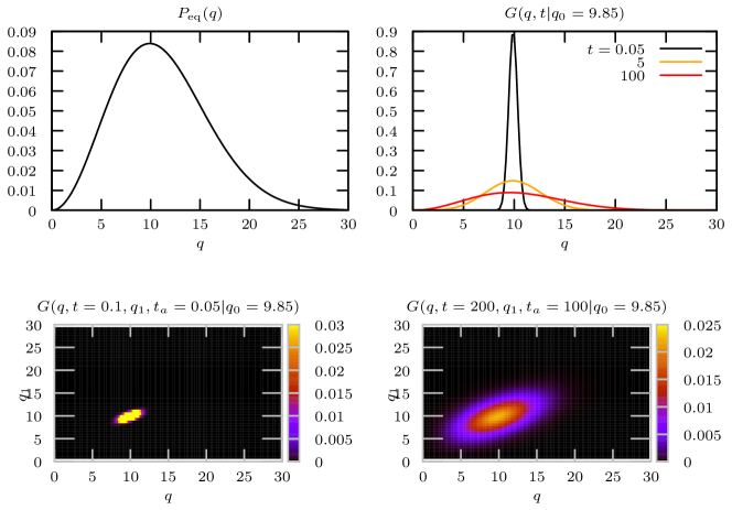
Figure D1: The top left panel shows the density of the invariant measure $P_{\mathrm{eq}}(q)$, while the top right panel depicts the conditional two-point density $G_{\mathrm{eq}}(q,t|q_{0})$ in Eq. (D16) for $q_{0}=9.85$ and three different $t$. The bottom panels show the conditional three-point probability density function $G_{\mathrm{eq}}(q,\tau+t_{a},q^{\prime},t_{a}|q_{0})$ in Eq. (D24) for two combinations of $t=\tau+t_{a}$ and $t_{a}$.

The density of the invariant measure of the end-to-end distance, $P_{\mathrm{eq}}(q)$ (Fig. D1, top left) is concentrated in the regime $0<q<30$ with a maximum at $q_{\mathrm{peak}}=9.85\approx 10$. The evolution of the conditional two-point conditional probability density for an ensemble of trajectories starting at the typical distance $q_{\mathrm{peak}}$, $G_{\mathrm{eq}}(q,t|q_{\mathrm{peak}})$ (Fig. D1, top right) evolves smoothly towards $P_{\mathrm{eq}}(q)$ with a relaxation time $t_{\mathrm{rel}}=\lambda_{1}^{-1}\approx 253.4$. Notably, the corresponding three-point density $G_{\mathrm{eq}}(q,t,q^{\prime},t_{a}|q_{\mathrm{peak}})$ (Fig. D1, bottom) shows strong long-time correlations in the evolution of $q(t)$, e.g. even for aging times $t_{a}=100$ (which are already of the order of, but still smaller than, $t_{\mathrm{rel}}$) the value of $q$ at time $t=2t_{a}$ is strongly correlated with its value $q^{\prime}$ at $t_{a}$ (Fig. D1, bottom right). This long-lasting correlations, which are the result of the projection of the full $3(N+1)$-dimensional dynamics of the polymer onto a single distance coordinate $q(t)$, are responsible for the dynamical time asymmetry.

Note that the relaxation time scales quadratically with the length of the chain, in.e. $t_{\mathrm{rel}}\propto N^{2}$ and therefore the dynamical time asymmetry extends, for long polymers $N\gtrsim 10^{4}$ over many orders in time. However, for such long chains the computation or $\Upsilon$ at short $t_{a},\tau$ becomes numerically unstable. In Fig. D2 we demonstrate the quadratic growth of relaxation time-scales displaying dynamical time asymmetry with increasing $N$.

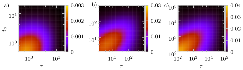
Figure D2: $\Upsilon(t_{a},\tau)$ for a) $N=10$, b) $N=10^{2}$, and c) $N=10^{3}$ portraying a growing time-scale of dynamical time asymmetry.

D.3 Single file diffusion

The single file model refers to the overdamped Brownian motion of a system of $N$ particles with hard core exclusion interactions, which for simplicity (and because the finite-size scenario is obtained by a simple re-scaling of space) we assume to be point-like and confined to an interval of unit length $L=1$ [124, 125, 101]. We express length in units of $L$ and time in units of $\tau=D/L^{2}$, where $D$ corresponds to the diffusion coefficient which is assumed to be equal for all particles. The state of the system is completely described with the vector of particle positions $\mathbf{x}=(x_{1},\ldots,x_{N})$. We are interested in tagged-particle dynamics and therefore our projected observable corresponds to the position of the $i$-th particle, $q(t)=x_{i}(t)$. The full system’s dynamics is driven solely by entropic driving forces because the potential energy is strictly zero. In turn, the free energy landscape (i.e. the potential of the mean force acting on the tagged particle) corresponds to the entropic landscape, whereas the potential energy hypersurface is perfectly flat.

The Fokker-Planck equation for the Green’s function with initial condition $Q(\mathbf{x},t=0|\mathbf{x}_{0})$ describing the dynamics of $N$ reads

$$(\partial_{t}-\sum_{i}\partial^{2}_{x_{i}})Q(\mathbf{x},t|\mathbf{x}_{0})=0,\quad Q(\mathbf{x},t=0|\mathbf{x}_{0})=\prod_{i=1}^{N}\delta(x_{i,0}-x_{i}),$$ (D27)

which is solved under $N-1$ non-crossing boundary conditions

$$\lim_{x_{i+1}\to x_{i}}(\partial_{x_{0,i+1}}-\partial_{x_{0,i}})Q(\mathbf{x},t|\mathbf{x}_{0})=0,\quad\forall i.$$ (D28)

The system is exactly solvable with the coordinate Bethe ansatz, which yields explicit results for the spectral expansion of $Q(\mathbf{x},t|\mathbf{x}_{0})$ [125, 101], i.e. $Q(\mathbf{x},t|\mathbf{x}_{0})=\sum_{\mathbf{k}}\psi_{\mathbf{k}}^{R}(\mathbf{x})\psi_{\mathbf{k}}^{L}(\mathbf{x}_{0})\mathrm{e}^{-\lambda_{\mathbf{k}}t}$ according to Eq. (A4), where we introduced the $N$-tuple $\mathbf{k}=(k_{1},\ldots,k_{N}),k_{i}\in\mathbb{N},\forall i$. Expressions for the eigenfunctions $\psi_{\mathbf{k}}^{R}(\mathbf{x}),\psi_{\mathbf{k}}^{L}(\mathbf{x})$ are given in [125, 101] and the eignevalues corresponding to $\lambda_{\mathbf{k}}=\sum_{i=1}^{N}k_{i}\pi^{2}$. Note that the relaxation time $t_{\rm rel}=1/\lambda_{\mathbf{1}}$ once re-scaled to natural units in terms of the collision time (i.e. $t_{\rm col}=(L/N)^{2}/D$ scales as $\propto N^{2}$.

The projection operator is turn defined by Eq. (B1) with $\delta(x_{i}-q)$, which according to Eq. (B7) yields, upon some tedious algebra, $G_{\mathrm{eq}}(q,t|q_{0}\in\Xi_{0})$ in Eq. (B10) and $G_{\mathrm{eq}}(q,t,q^{\prime},t_{a}|q_{0}\in\Xi_{0})$ in Eq. (B21) with matrix elements

$$\Psi_{\mathbf{kl}}(x)=\frac{\mathbf{m_{l}}!}{N_{L}!N_{R}!}\sum_{\{n_{i}\}}T_{j}(x)\prod_{i=1}^{j-1}L_{i}(x)\prod_{i=j+1}^{N}R_{i}(x)$$ (D29)

where $\mathbf{m_{l}}!=\prod_{i}m_{k_{i}}$ is the multiplicity of the eigenstate with $m_{k_{i}}$ corresponds to the number of times a particular value of $k_{1}$ appears in the tuple and $N_{L},N_{R}$ are the number of particles to the left and right from the tagged particle, respectively. The sum $\sum_{\{n_{i}\}}$ is over all permutations of the elements of the $N$-tuple $\mathbf{k}$. For the equilibrium density we find $P_{\mathrm{eq}}(q)=\frac{N!}{N_{L}!N_{R}!}q^{N_{L}}(1-q)^{N_{R}}$. In Eq. (D29) we have defined the auxiliary functions

$$T_{j}(x) = \begin{cases}1\quad\lambda_{k}=\lambda_{l}=0\\ \displaystyle{\sqrt{2}\cos(\lambda_{k/l}\pi x)}\quad\lambda_{k}=0\,\text{or}\,\lambda_{l}=0\\ \displaystyle{2\cos(\lambda_{k}\pi x)\cos(\lambda_{l}\pi x)}\quad\text{otherwise}\\ \end{cases}$$ (D30)

$$L_{j}(x) = \begin{cases}x\quad\lambda_{k}=\lambda_{l}=0\\ \displaystyle{\sqrt{2}\frac{\sin(\lambda_{k/l}\pi x)}{\lambda_{k/l}\pi}\quad\lambda_{k}=0}\,\text{or}\,\lambda_{l}=0\\ \displaystyle{x+\frac{\sin(2\lambda_{k}\pi x)}{2\lambda_{k}\pi x}}\quad\lambda_{k}=\lambda_{l}\\ \displaystyle{2\frac{\lambda_{k}\cos(\lambda_{l}\pi x)\sin(\lambda_{k}\pi x)-\lambda_{l}\cos(\lambda_{k}\pi x)\sin(\lambda_{l}\pi x)}{\pi(\lambda_{k}^{2}-\lambda_{l}^{2})}}\quad\text{otherwise}\\ \end{cases}$$ (D32)

$$R_{j}(x) = \begin{cases}\displaystyle{1-x}\quad\lambda_{k}=\lambda_{l}=0\\ \displaystyle{-\sqrt{2}\frac{\sin(\lambda_{k/l}\pi x)}{\lambda_{k/l}\pi}}\quad\lambda_{k}=0\,\text{or}\,\lambda_{l}=0\\ \displaystyle{1-x-\frac{\sin(2\lambda_{k}\pi x)}{2\lambda_{k}\pi x}}\quad\lambda_{k}=\lambda_{l}\\ \displaystyle{2\frac{-\lambda_{k}\cos(\lambda_{l}\pi x)\sin(\lambda_{k}\pi x)+\lambda_{l}\cos(\lambda_{k}\pi x)\sin(\lambda_{l}\pi x)}{\pi(\lambda_{k}^{2}-\lambda_{l}^{2})}}\quad\text{otherwise}\\ \end{cases}$$ (D33)

The autocorrelation functions $C(t)$ and $C_{t_{a}}(\tau)$ can now be calculated using Eqs. (B14) and (B16), respectively, where trivially $\langle q(t)\rangle=(N_{l}+1)/(N+1)$ and $\langle q(0)^{2}\rangle=(N_{L}+2)(N_{L}+1)/[(N+2)(N+1)]$. As it was impossible to carry out this final step analytically, we carried out the integrals in Eqs. (B14) and (B16) depicted in Fig. 3b in the main text numerically according to the trapezoidal rule.

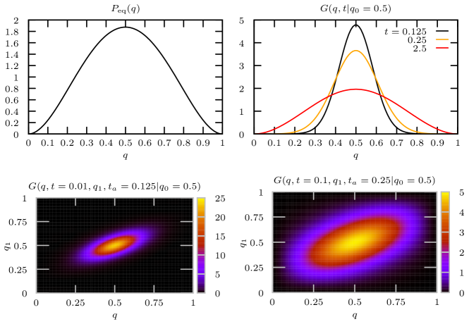
Figure D3: Single file. The top left panel depicts the density of the equilibrium measure $P_{\mathrm{eq}}(q)$ of the third particle in a single file of five particles, $q(t)=x_{3}(t)$. The top right panel shows a two-point conditional probability density function $G(q,t|q_{0})$ for different values of $t$, where $q_{0}=0.5$ (i.e. the maximum of the $P_{\mathrm{eq}}(q)$). The bottom panels depict the three-point density $G(q,t,q^{\prime},t_{a}|q_{0})$ at different $\tau$ and $t_{a}$ evolving from the same initial condition. To produce $G(q,t,q^{\prime},t_{a}|q_{0})$ the spectral expansion Eq. (A4) was truncated at maximum Bethe eigenvalue $225\pi^{2}$.

The computation of the time asymmetry index $\Upsilon$ in Eq. (B25), which was as well performed using the trapezoidal rule on a grid of 100 points, is extremely challenging even for moderate values of $N$. By repeating the integration using a smaller grid of 50 points we double-checked that the integration routine converged to a sufficient degree. The results for a single file of $N=5$ particles tagging the third particle are presented in Fig. 3b in the main text and in Fig. D3.

The density of the invariant measure of the tagged central particle (Fig. D3, top left) peaks in the center of the unit box, $q_{\mathrm{peak}}=0.5$, and decays towards the borders due to the entropic repulsion with the neighbors. The evolution of the conditional two-point conditional probability density for an ensemble of trajectories starting at the typical distance $q_{\mathrm{peak}}$, $G_{\mathrm{eq}}(q,t|q_{\mathrm{peak}})$ (Fig. D3, top right) evolves smoothly towards $P_{\mathrm{eq}}(q)$ with a relaxation time $t_{\mathrm{rel}}=\lambda_{1}^{-1}\approx 2.5$.

Similar to the end-to-end distance of the Rouse polymer the corresponding three-point density of the tagged particle, $G_{\mathrm{eq}}(q,t,q^{\prime},t_{a}|q_{\mathrm{peak}})$ (Fig. D3, bottom) shows strong long-time correlations in the evolution of $q(t)$, e.g. even for aging times $t_{a}=0.125$ (which are already of the order of, but still smaller than, $t_{\mathrm{rel}}$) the value of $q$ at time $t=2t_{a}$ is strongly correlated with its value $q^{\prime}$ at $t_{a}$ (Fig. D1, bottom right). This long-lasting correlation reflects prolonged entropic bottlenecks (i.e. ’traffic-jams’), which require collective rearrangements of many particles and thus decorrelate slowly, giving rise to strong memory effects and dynamical time asymmetry (see Fig. 3b in the main text) as soon as $q_{0}$ is initially not sampled from $P_{\mathrm{eq}}(q_{0})$.

D.4 Analysis of experimental and simulation data

We now consider the time series of a low-dimensional projected observable sampled at discrete time steps that is frequently encountered in the analysis of experimental data. Therefore we first translate all definitions in Sec. B to discrete time series and explain in detail how to carry out the complete analysis of aging dynamics for such systems. To ease the application of these new concepts we also provide a C++ routine TSymmetryFinder that will be made available on GitHub.

We consider a discrete time series of length $N$ – in our case a one-dimensional physical observable $q(t_{i})$ – sampled at constant time intervals with spacing $t_{i+1}-t_{i}=\Delta t,\forall i$. We pre-process the data by evaluating the mean value over the time series $\overline{q}=N^{-1}\sum_{i=1}^{N}q(t_{i})$ and then center the data by subtracting the mean value, $q(t_{i})\to q(t_{i})-\overline{q}$. In the first stage we determine the (non-aging) autocorrelation function

$$C(\tau=n_{\tau}\Delta t)=\frac{1}{(N-n_{\tau})\Delta t}\sum_{i=1}^{N-n_{\tau}}q(t_{i+n_{\tau}})q(t_{i})\Delta t,\qquad n_{\tau}\ll N$$ (D34)

and determine the relaxation time as $t_{r}:\displaystyle{\min_{t_{i}}}[\mathcal{C}(t_{i})/\mathcal{C}(0)<\epsilon]$, where we choose $\epsilon=0.05$. All data are henceforth analyzed such that $n_{\mathrm{max}}\equiv n_{\tau_{max}}\approx n_{r}=t_{r}/(\Delta t)$ in order to assure sufficient sampling when evaluating sliding averages.

Next we determine the equilibrium probability density function and two-point conditional probability density (Eq. (B2)) as a histogram taken over the data. We introduce bins $\mathcal{B}_{i}$ centered at $q_{i}$ with a width $\delta q$ and define the characteristic function of a bin $\mathbbm{1}_{\mathcal{B}_{i}}[q(t_{i})]=1$ if $q_{i}-\delta q/2\leq q(t_{i})<q_{i}+\delta q/2$ and zero otherwise and let $\mathbbm{1}_{\Xi_{0}}[q]$ be the indicator function of the initial condition. Let us further define $n_{l}(n_{\tau})=\displaystyle{\max_{i}q(t_{i})\in\Xi_{0}}:n_{l}+n_{\tau}\leq N$. The equilibrium probability density function is then determined as

$$P_{\mathrm{eq}}(q_{i})=(N\delta q)^{-1}\sum_{i=1}^{N}\mathbbm{1}_{\mathcal{B}_{i}}[q(t_{i})]$$ (D35)

and the 2-point conditional probability density as

$$G(q_{i},n_{\tau}|q_{0}\in\Xi_{0}) = \frac{\sum_{i=1}^{n_{l}(n_{\tau})}\mathbbm{1}_{\mathcal{B}_{i}}[q(t_{i+n_{\tau}})]\mathbbm{1}_{\Xi_{0}}[q(t_{i})]}{\delta q\sum_{i=1}^{n_{l}(n_{\tau})}\mathbbm{1}_{\Xi_{0}}[q(t_{i})]},$$ (D36)

$$G(q_{i},n_{\tau}|q_{j}) = \frac{\sum_{i=1}^{n_{l}(n_{\tau})}\mathbbm{1}_{\mathcal{B}_{i}}[q(t_{i+n_{\tau}})]\mathbbm{1}_{\mathcal{B}_{j}}[q(t_{i})]}{\delta q\sum_{i=1}^{n_{l}(n_{\tau})}\mathbbm{1}_{\Xi_{0}}[q(t_{i})]},$$ (D37)

The three-point conditional density Eq. (B21) is defined for $n_{\tau^{\prime}}\leq n_{\tau}$ analogously as

$$G(q_{i},n_{\tau},q_{j},n_{\tau^{\prime}}|q_{0}\in\Xi_{0})=\frac{\sum_{i=1}^{n_{l}(n_{\tau})}\mathbbm{1}_{\mathcal{B}_{i}}[q(t_{i+n_{\tau}})]\mathbbm{1}_{\mathcal{B}_{j}}[q(t_{i+n_{\tau^{\prime}}})]\mathbbm{1}_{\Xi_{0}}[q(t_{i})]}{\delta q^{2}\sum_{i=1}^{n_{l}(n_{\tau})}\mathbbm{1}_{\Xi_{0}}[q(t_{i})]}.$$ (D38)

Introducing $\delta n=n_{\tau}-n_{a}$ the time-asymmetry index is in turn determined as a double sum

$$\Upsilon_{\Xi_{0}}(t_{a},\tau)=\delta q^{2}\sum_{i,j}G(q_{i},\delta n+n_{a},q_{j},n_{a}|q_{0}\in\Xi_{0})\log\frac{G(q_{i},\delta n+n_{a},q_{j},n_{a}|q_{0}\in\Xi_{0})}{G(q_{i},\delta n+n_{a}|q_{j})G(q_{i},n_{a}|q_{0}\in\Xi_{0})},$$ (D39)

whereas the normalized aging correlation function (Eq. (B16) is determined according to

$$\hat{C}_{t_{a}}(\tau) = \frac{\langle q(t_{\delta n+n_{a}})q(t_{n_{a}})\rangle-\langle q(t_{\delta n+n_{a}})\rangle\langle q(t_{n_{a}})\rangle}{\langle q^{2}(t_{n_{a}})\rangle-\langle q(t_{n_{a}})\rangle^{2}},$$ (D40)

$$\langle q(t_{\delta n+n_{a}})q(t_{n_{a}})\rangle \equiv \sum_{i,j}q_{i}q_{j}G(q_{i},\delta n+n_{a},q_{j},n_{a}|q_{0}\in\Xi_{0}),$$ (D41)

$$\langle q(t_{i})\rangle \equiv \sum_{i,j}q_{i}G(q_{i},n_{i}|q_{0}\in\Xi_{0}),$$ (D42)

where $\tau=\delta n\Delta t$ and $t_{a}=n_{a}\Delta t$ and we note that by construction (i.e. due to the centering of data) $\langle q(t_{i})\rangle=0,\forall i$. 100 bins in $q(t_{\delta n+n_{a}})$ and 100 bins in $q(t_{n_{a}})$ were used for each combination of $\tau$ and $t_{a}$ to determine $G(q_{i},\delta n+n_{a},q_{j},n_{a}|q_{0}\in\Xi_{0}),G(q_{i},\delta n+n_{a}|q_{j})$ and $G(q_{i},n_{a}|q_{0}\in\Xi_{0})$ and in turn $\Upsilon_{\Xi_{0}}(t_{a},\tau)$.

D.4.1 DNA-hairpin

Dual optical tweezers data of the DNA hairpin were kindly provided by the Woodside group [69] in the form of a constant trap measurements of the DNA hairpin 30R50T4, sampled at $400$ kHz, for trap stiffness $0.63pN/nm$ in one optical trap and $1.1pN/nm$ in the other. The time series was $2.75\cdot 10^{4}\mathrm{ms}$ long. The normalized aging correlation function $C_{t_{a}}(\tau)$ and dynamical time asymmetry index $\Upsilon$ are depicted in Figs. 3c and 4b in the manuscript. Here, we additionally present in Fig. D4, for illustrative purposes and for the sake of completeness, the density of the invariant (equilibrium) measure $P_{\mathrm{eq}}(q)$ and exemplary two-point conditional probability $G(q,t|q_{0}\in\Xi_{0})$ and the three-point conditional density $G(q,\tau+t_{a},q^{\prime},t_{a}|q_{0}\in\Xi_{0})$, respectively, for various $t$. The histograms in the relative deviations $q(t_{i})=q_{\mathrm{raw}}(t_{i})-\overline{q}$ were determined by binning the interval from -25 nm to +15 nm into 100 bins and $\overline{q}=3.47$ nm. These probability density functions are shown in Fig. D4.

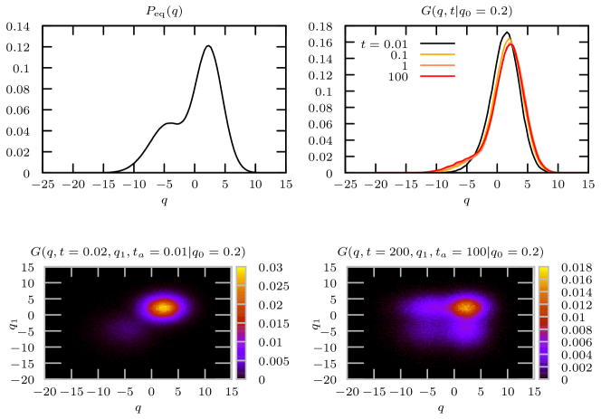
Figure D4: DNA Hairpin. In the top left panel depicts the density of the equilibrium measure $P_{\mathrm{eq}}(q)$ of the centered time series $q(t_{i})=q_{\mathrm{raw}}(t_{i})-\overline{q}$, while the top right shows a two-point conditional probability density function $G(q,t|q_{0}\in\Xi_{0})$ for different values of $t$, where $\Xi_{0}=[0.2-0.2,0.2+0.2]$ nm. The bottom panels depict the three-point density $G(q,t,q^{\prime},t_{a}|q_{0}\in\Xi_{0})$ at different $\tau$ and $t_{a}$ evolving from the same initial condition.

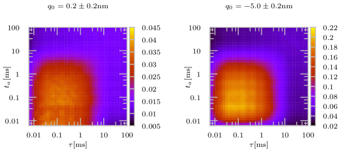
Figure D5: DNA Hairpin, second example. The time asymmetry index for the DNA hairpin data as in Fig. D4 but with the initial condition $\Xi_{0}=[-5-0.2,-5+0.2]$ nm.

The density of the invariant measure of the extension of the hairpin is bimodal, reflecting the existence of two long-lived conformational states (Fig. D5, top left). The evolution of the conditional two-point conditional probability density for an ensemble of trajectories starting at the typical distance $q_{\mathrm{peak}}$, $G_{\mathrm{eq}}(q,t|q_{\mathrm{peak}})$ (Fig. D5, top right) evolves smoothly towards $P_{\mathrm{eq}}(q)$ with a relaxation time $t_{\mathrm{rel}}=\lambda_{1}^{-1}\approx 15ms$, and nicely depicts the onset of conformational transitions (see red line).

Another striking feature of hairpin dynamics is seen in the corresponding three-point density, $G_{\mathrm{eq}}(q,t,q^{\prime},t_{a}|q_{\mathrm{peak}})$ (Fig. D5, bottom), which depicts, alongside the linear correlations along and near the diagonal $q=q^{\prime}$ that were also present in the Rouse polymer and tagged-particle diffusion in a single-file, prominent non-linear correlations (see off-diagonal peaks). This readily reveals that temporal correlations in the motion persist beyond the time-scale of conformational transitions, that is, the hairpin relaxation dynamics post transition remembers the configurations prior to the transition even on time-scales of $\gtrsim 200$ ms, which reflects a very long range of broken Markovianity. However, a comparison with the corresponding time asymmetry index in Fig. 3c in the main text shows that at aging times $t_{a}=100$ ms the dynamics is already time-translation invariant. This is a nice and clear practical demonstration of the important conceptual difference between the notion of relaxation with a broken time-translation invariance and memory effects in time-translation invariant relaxation of a low-dimensional physical observable.

In order to demonstrate the robustness of these observations with respect to specific the initial condition $q_{0}=1(0)$ (as long as $p_{0}(q_{0})\neq P_{\mathrm{eq}}(q_{0})$ that is) we also present in Fig. D5 the results for a different set of initial conditions. The results in Fig. D5 show qualitatively the same features and are fully consistent with the statements in the manuscript.

Finally, we asses the statistical uncertainty of determining $\Upsilon$ from the experimental time-series. We do so by performing the analysis on an ensemble of trajectories obtained by randomly removing 10 (from the total of 50, i.e. $20$% of the data) trajectories and averaging over 20 repetitions of a data-set created in this manner. We quantify the statistical error by determining the local standard deviation of $\Upsilon$, i.e. $\sigma_{\Upsilon}=\sqrt{N_{i}^{-1}\sum_{i=1}^{N_{i}}\Upsilon_{i}^{2}-(N_{i}^{-1}\sum_{i=1}^{N_{i}}\Upsilon_{i})^{2}}$ where $N_{i}$=20. The results are shown in Fig. D6 and depict a local error that is smaller than 1%.

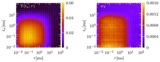
Figure D6: Statistical error in the DNA-hairpin analysis. a) average $\Upsilon(\tau,t_{a})$ determined from an ensemble with forced under-sampling (i.e. by omiting 20% of the data); b) the standard deviation of the local $\Upsilon(\tau,t_{a})$.

D.4.2 Yeast 3-phosphoglycerate kinase (PGK)

Atomistic Molecular Dynamics (MD) simulation of yeast PGK were carried out by Hu et al. [39], starting from the PDB structure 3PGK with a duration of $1.71\cdot 10^{5}\mathrm{ps}$. The observable $q(t_{i})$ refers here to the distance between the center of mass of the N-terminal domain (residues 1-185) and the center of mass of C-terminal domain (residues 200-389). In Fig. D7 we depict the density of the invariant (equilibrium) measure $P_{\mathrm{eq}}(q)$ and exemplary two-point conditional probability $G(q,t|q_{0}\in\Xi_{0})$ and the three-point conditional density $G(q,\tau+t_{a},q^{\prime},t_{a}|q_{0}\in\Xi_{0})$, respectively, for various $t$. The histograms in the relative deviations $q(t_{i})=q_{\mathrm{raw}}(t_{i})-\overline{q}$ were determined by binning the interval from -0.2 nm to +0.3 nm into 100 bins and $\overline{q}=0.67$ nm.

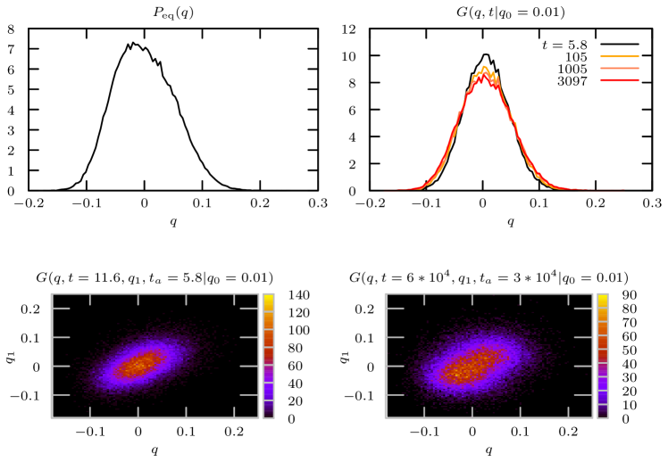
Figure D7: PGK. The top left panel depicts the density of the equilibrium measure $P_{\mathrm{eq}}(q)$ of the centered time series $q(t_{i})=q_{\mathrm{raw}}(t_{i})-\overline{q}$, while the top right shows a two-point conditional probability density function $G(q,t|q_{0}\in\Xi_{0})$ for different values of $t$, where $\Xi_{0}=[0.01-0.005,0.01+0.005]$ nm. The bottom panels depict the three-point density $G(q,t,q^{\prime},t_{a}|q_{0}\in\Xi_{0})$ at different $\tau$ and $t_{a}$ evolving from the same initial condition.

The density of the invariant measure $P_{\mathrm{eq}}(q)$ (Fig. D7, top left) is unimodal and effects of a poorer statistics are readily discernable through the roughness of the curve. The evolution of the conditional two-point conditional probability density for an ensemble of trajectories starting at the typical distance $q_{\mathrm{peak}}$, $G_{\mathrm{eq}}(q,t|q_{\mathrm{peak}})$ is shown in Fig. D7 (top right panel) and reveals that the the dynamics along $q$ is strongly localized (i.e. $G_{\mathrm{eq}}(q,t|q_{\mathrm{peak}}$ barely changes between $t=100$ ps and $t=3000$). Note that PGK did not relax within the duration of the trajectory. The corresponding three-point density, $G_{\mathrm{eq}}(q,t,q^{\prime},t_{a}|q_{\mathrm{peak}})$ (Fig. D7, bottom), shows that the observable almost does not relax at all within $6\times 10^{4}$ ps (compare left and right panel). As in the case of the Rouse polymer $G_{\mathrm{eq}}(q,t,q^{\prime},t_{a}|q_{\mathrm{peak}})$ shows strong and long-lasting correlations between positions, and comparison with the dynamical time asymmetry index in Fig. 3d in the main text reveals that the dynamics has a strongly time-translation invariance. These findings corroborate the original analysis of Hu et al. [39] who observed aging effects.

Similar to the DNA hairpin we also present in Fig. D8 the results for the dynamical time asymmetry index for a different set of initial conditions and two different choices of the observable $q(t)$ for PGK, which demonstrate the robustness of the results.

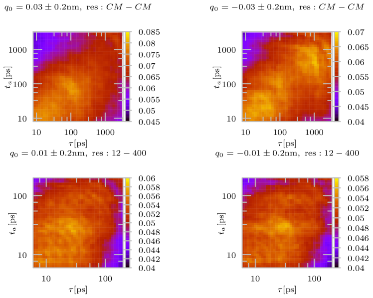
Figure D8: PGK, second example. Top: dynamical time asymmetry index for yeast PGK when $q(t)$ corresponds to distance between the center of masses of the N- and C- terminal domains (respectively residues 1-185 and 200-389) for a pair different initial conditions. Bottom: dynamical time asymmetry index for yeast PGK when $q(t)$ corresponds to the distance between two specific residues (the 12th and the 400th) for two different initial conditions.

PGK obviously does not relax within the duration of the trajectory and more generally it is conceivable that larger, complex proteins do not relax at all during their life-time [39], which makes them virtually ’forever aging’ [126], which may have important consequences for their biological function. Such aging effects on function were observabed in single-enzyme turnover statistics [41, 42, 43] and have so-far been rationalized only with ad-hoc phenomenological models [42, 43]. The present theoretical framework provides a unifying mechanistic understanding dynamics with broken time-translation invariance in soft and biological matter and will pave the way for deeper and more systematic investigations of the potential biological relevance of memory and dynamical time asymmetry for enzymatic catalysis.

References

- Farhan et al. [2013] A. Farhan, P. M. Derlet, A. Kleibert, A. Balan, R. V. Chopdekar, M. Wyss, J. Perron, A. Scholl, F. Nolting, and L. J. Heyderman, Direct Observation of Thermal Relaxation in Artificial Spin Ice, Phys. Rev. Lett. 111, 057204 (2013).
- Dattagupta [2012] S. Dattagupta, Relaxation phenomena in condensed matter physics (Elsevier, 2012).
- Kubo et al. [1991] R. Kubo, M. Toda, and N. Hashitsume, Statistical Physics II (Springer Berlin Heidelberg, 1991).
- Chen et al. [2007] H. Chen, E. Rhoades, J. S. Butler, S. N. Loh, and W. W. Webb, Dynamics of equilibrium structural fluctuations of apomyoglobin measured by fluorescence correlation spectroscopy, Proc. Natl. Acad. Sci. USA 104, 10459–10464 (2007).
- Onsager [1931a] L. Onsager, Reciprocal relations in irreversible processes. i., Phys. Rev. 37, 405 (1931a).
- Onsager [1931b] L. Onsager, Reciprocal relations in irreversible processes. ii., Phys. Rev. 38, 2265 (1931b).
- Kubo et al. [1957] R. Kubo, M. Yokota, and S. Nakajima, Statistical-mechanical theory of irreversible processes. ii. response to thermal disturbance, J. Phys. Soc. Jpn. 12, 1203–1211 (1957).
- Metzler et al. [1999] R. Metzler, E. Barkai, and J. Klafter, Anomalous diffusion and relaxation close to thermal equilibrium: A fractional fokker-planck equation approach, Phys. Rev. Lett. 82, 3563 (1999).
- Maes et al. [2011] C. Maes, K. Netočný, and B. Wynants, Monotonic Return to Steady Nonequilibrium, Phys. Rev. Lett. 107, 010601 (2011).
- Baiesi and Maes [2013] M. Baiesi and C. Maes, New J. Phys. 15, 013004 (2013).
- Polettini and Esposito [2013] M. Polettini and M. Esposito, Nonconvexity of the relative entropy for Markov dynamics: A Fisher information approach, Phys. Rev. E 88, 012112 (2013).
- Maes [2017] C. Maes, Phys. Rev. Lett. 119, 160601 (2017).
- Maes [2020] C. Maes, Frenesy: Time-symmetric dynamical activity in nonequilibria, Phys. Rep. 850, 1 (2020).
- Kurchan [2005] J. Kurchan, In and out of equilibrium, Nature 433, 222–225 (2005).
- Cugliandolo et al. [1997] L. F. Cugliandolo, D. S. Dean, and J. Kurchan, Fluctuation-dissipation theorems and entropy production in relaxational systems, Phys. Rev. Lett. 79, 2168 (1997).
- Lu and Raz [2017] Z. Lu and O. Raz, Nonequilibrium thermodynamics of the Markovian Mpemba effect and its inverse, Proc. Natl. Acad. Sci. USA 114, 5083 (2017).
- Klich et al. [2019] I. Klich, O. Raz, O. Hirschberg, and M. Vucelja, Phys. Rev. X 9, 021060 (2019).
- Shiraishi and Saito [2019] N. Shiraishi and K. Saito, Information-Theoretical Bound of the Irreversibility in Thermal Relaxation Processes, Phys. Rev. Lett. 123, 110603 (2019).
- Lapolla and Godec [2020] A. Lapolla and A. Godec, Faster uphill relaxation in thermodynamically equidistant temperature quenches, Phys. Rev. Lett. 125, 110602 (2020).
- Bouchaud [1992] J. P. Bouchaud, Weak ergodicity breaking and aging in disordered systems, J. de Physique I 2, 1705–1713 (1992).
- [21] E. Vincent, J. Hammann, M. Ocio, J.-P. Bouchaud, and L. F. Cugliandolo, Slow dynamics and aging in spin glasses, Lecture Notes in Physics , 184–219.
- Bouchaud et al. [1997] J.-P. Bouchaud, L. F. Cugliandolo, J. Kurchan, and M. Mézard, Out of equilibrium dynamics in spin-glasses and other glassy systems, in Spin Glasses and Random Fields (World Scientific, 1997) pp. 161–223.
- Monthus and Bouchaud [1996] C. Monthus and J.-P. Bouchaud, Models of traps and glass phenomenology, J. Phys. A: Math. Gen. 29, 3847–3869 (1996).
- J.-P. Bouchaud and D.S. Dean [1995] J.-P. Bouchaud and D.S. Dean, Aging on parisi’s tree, J. Phys. I France 5, 265 (1995).
- Ritort and Sollich [2003] F. Ritort and P. Sollich, Glassy dynamics of kinetically constrained models, Adv. Phys. 52, 219 (2003).
- Hodge [1995] I. M. Hodge, Physical aging in polymer glasses, Science 267, 1945–1947 (1995).
- Oukris and Israeloff [2009] H. Oukris and N. E. Israeloff, Nanoscale non-equilibrium dynamics and the fluctuation–dissipation relation in an ageing polymer glass, Nat. Phys. 6, 135–138 (2009).
- Hérisson and Ocio [2002a] D. Hérisson and M. Ocio, Fluctuation-dissipation ratio of a spin glass in the aging regime, Phys. Rev. Lett. 88, 257202 (2002a).
- Kenning et al. [2006] G. G. Kenning, G. F. Rodriguez, and R. Orbach, End of aging in a complex system, Phys. Rev. Lett. 97, 057201 (2006).
- Mattsson et al. [2009] J. Mattsson, H. M. Wyss, A. Fernandez-Nieves, K. Miyazaki, Z. Hu, D. R. Reichman, and D. A. Weitz, Soft colloids make strong glasses, Nature 462, 83–86 (2009).
- Cipelletti et al. [2000] L. Cipelletti, S. Manley, R. C. Ball, and D. A. Weitz, Universal aging features in the restructuring of fractal colloidal gels, Phys. Rev. Lett. 84, 2275 (2000).
- Lunkenheimer et al. [2005] P. Lunkenheimer, R. Wehn, U. Schneider, and A. Loidl, Glassy aging dynamics, Phys. Rev. Lett. 95, 055702 (2005).
- Lubchenko and Wolynes [2007] V. Lubchenko and P. G. Wolynes, Theory of structural glasses and supercooled liquids, Annu. Rev. Phys. Chem. 58, 235 (2007).
- Castillo and Parsaeian [2006] H. E. Castillo and A. Parsaeian, Local fluctuations in the ageing of a simple structural glass, Nat. Phys. 3, 26–28 (2006).
- Utz et al. [2000] M. Utz, P. G. Debenedetti, and F. H. Stillinger, Atomistic simulation of aging and rejuvenation in glasses, Phys. Rev. Lett. 84, 1471 (2000).
- Frauenfelder et al. [1991] H. Frauenfelder, S. Sligar, and P. Wolynes, The energy landscapes and motions of proteins, Science 254, 1598–1603 (1991).
- Brujić et al. [2006] J. Brujić, R. I. Hermans Z., K. A. Walther, and J. M. Fernandez, Single-molecule force spectroscopy reveals signatures of glassy dynamics in the energy landscape of ubiquitin, Nat. Phys. 2, 282–286 (2006).
- Morgan et al. [2020] I. L. Morgan, R. Avinery, G. Rahamim, R. Beck, and O. A. Saleh, Glassy dynamics and memory effects in an intrinsically disordered protein construct, Phys. Rev. Lett. 125, 058001 (2020).
- Hu et al. [2015] X. Hu, L. Hong, M. Dean Smith, T. Neusius, X. Cheng, and J. Smith, The dynamics of single protein molecules is non-equilibrium and self-similar over thirteen decades in time, Nat. Phys. 12, 171–174 (2015).
- Xue and Yeung [1995] Q. Xue and E. S. Yeung, Differences in the chemical reactivity of individual molecules of an enzyme, Nature 373, 681–683 (1995).
- Lu et al. [1998] H. P. Lu, L. Xun, and X. S. Xie, Single-molecule enzymatic dynamics, Science 282, 1877 (1998).
- van Oijen et al. [2003] A. M. van Oijen, P. C. Blainey, D. J. Crampton, C. C. Richardson, T. Ellenberger, and X. S. Xie, Single-molecule kinetics of exonuclease reveal base dependence and dynamic disorder, Science 301, 1235 (2003).
- English et al. [2005] B. P. English, W. Min, A. M. van Oijen, K. T. Lee, G. Luo, H. Sun, B. J. Cherayil, S. C. Kou, and X. S. Xie, Ever-fluctuating single enzyme molecules: Michaelis-menten equation revisited, Nat. Chem. Biol. 2, 87–94 (2005).
- Keim et al. [2019] N. C. Keim, J. D. Paulsen, Z. Zeravcic, S. Sastry, and S. R. Nagel, Memory formation in matter, Rev. Mod. Phys. 91, 035002 (2019).
- Burov et al. [2010] S. Burov, R. Metzler, and E. Barkai, Aging and nonergodicity beyond the khinchin theorem, Proc. Natl. Acad. Sci. 107, 13228 (2010).
- Franz and Hertz [1995] S. Franz and J. Hertz, Glassy transition and aging in a model without disorder, Phys. Rev. Lett. 74, 2114 (1995).
- Ritort [1995] F. Ritort, Glassiness in a model without energy barriers, Phys. Rev. Lett. 75, 1190 (1995).
- Cugliandolo et al. [1996] L. F. Cugliandolo, J. Kurchan, and P. Le Doussal, Large time out-of-equilibrium dynamics of a manifold in a random potential, Phys. Rev. Lett. 76, 2390 (1996).
- Amir et al. [2012] A. Amir, Y. Oreg, and Y. Imry, On relaxations and aging of various glasses, Proc. Natl. Acad. Sci. 109, 1850 (2012).
- Cugliandolo and Kurchan [1993] L. F. Cugliandolo and J. Kurchan, Analytical solution of the off-equilibrium dynamics of a long-range spin-glass model, Phys. Rev. Lett. 71, 173 (1993).
- Cugliandolo and Kurchan [1994] L. F. Cugliandolo and J. Kurchan, On the out-of-equilibrium relaxation of the sherrington-kirkpatrick model, J. Phys. A: Math. Gen. 27, 5749 (1994).
- Folena et al. [2020] G. Folena, S. Franz, and F. Ricci-Tersenghi, Rethinking mean-field glassy dynamics and its relation with the energy landscape: The surprising case of the spherical mixed -spin model, Phys. Rev. X 10, 031045 (2020).
- Franz et al. [1998] S. Franz, M. Mézard, G. Parisi, and L. Peliti, Measuring equilibrium properties in aging systems, Phys. Rev. Lett. 81, 1758 (1998).
- Mayer et al. [2006] P. Mayer, S. Léonard, L. Berthier, J. P. Garrahan, and P. Sollich, Activated aging dynamics and negative fluctuation-dissipation ratios, Phys. Rev. Lett. 96, 030602 (2006).
- Dechant et al. [2014] A. Dechant, E. Lutz, D. A. Kessler, and E. Barkai, Scaling green-kubo relation and application to three aging systems, Phys. Rev. X 4, 011022 (2014).
- Charbonneau et al. [2014] P. Charbonneau, J. Kurchan, G. Parisi, P. Urbani, and F. Zamponi, Fractal free energy landscapes in structural glasses, Nat. Commun. 5, 10.1038/ncomms4725 (2014).
- Cugliandolo et al. [1995] L. F. Cugliandolo, J. Kurchan, G. Parisi, and F. Ritort, Matrix models as solvable glass models, Phys. Rev. Lett. 74, 1012 (1995).
- Barkai [2003a] E. Barkai, Aging in subdiffusion generated by a deterministic dynamical system, Phys. Rev. Lett. 90, 104101 (2003a).
- Hartich and Godec [2018] D. Hartich and A. Godec, Duality between relaxation and first passage in reversible markov dynamics: rugged energy landscapes disentangled, New J. Phys. 20, 112002 (2018).
- Hartich and Godec [2019] D. Hartich and A. Godec, Interlacing relaxation and first-passage phenomena in reversible discrete and continuous space markovian dynamics, J. Stat. Mech. Theor. Exp. 2019, 024002 (2019).
- Speck and Seifert [2005] T. Speck and U. Seifert, Integral fluctuation theorem for the housekeeping heat, J. Phys. A: Math. Gen. 38, L581 (2005).
- Chétrite et al. [2019] R. Chétrite, S. Gupta, I. Neri, and É. Roldán, Martingale theory for housekeeping heat, EPL 124, 60006 (2019).
- Chun and Noh [2019] H.-M. Chun and J. D. Noh, Universal property of the housekeeping entropy production, Phys. Rev. E 99, 012136 (2019).
- Liu et al. [2020] K. Liu, Z. Gong, and M. Ueda, Thermodynamic uncertainty relation for arbitrary initial states, Phys. Rev. Lett. 125, 140602 (2020).
- Bovier and Faggionato [2005] A. Bovier and A. Faggionato, Spectral characterization of aging: The rem-like trap model, Ann. Appl. Probab. 15, 1997 (2005).
- Fielding et al. [2000] S. M. Fielding, P. Sollich, and M. E. Cates, Aging and rheology in soft materials, J. Rheol. 44, 323 (2000).
- Sollich et al. [1997] P. Sollich, F. m. c. Lequeux, P. Hébraud, and M. E. Cates, Rheology of soft glassy materials, Phys. Rev. Lett. 78, 2020 (1997).
- Neupane et al. [2017] K. Neupane, F. Wang, and M. T. Woodside, Direct measurement of sequence-dependent transition path times and conformational diffusion in dna duplex formation, Proc. Natl. Acad. Sci. 114, 1329 (2017).
- Neupane et al. [2018] K. Neupane, N. Q. Hoffer, and M. T. Woodside, Measuring the local velocity along transition paths during the folding of single biological molecules, Phys. Rev. Lett. 121, 018102 (2018).
- Solanki et al. [2014] A. Solanki, K. Neupane, and M. T. Woodside, Single-molecule force spectroscopy of rapidly fluctuating, marginally stable structures in the intrinsically disordered protein -synuclein, Phys. Rev. Lett. 112, 158103 (2014).
- Hyeon et al. [2014] C. Hyeon, M. Hinczewski, and D. Thirumalai, Evidence of disorder in biological molecules from single molecule pulling experiments, Phys. Rev. Lett. 112, 138101 (2014).
- Note [1] From a thermodynamic point of view such systems are characterized by a transiently positive entropy production that vanishes upon reaching equilibrium.
- Freidlin and Wentzell [2012] M. I. Freidlin and A. D. Wentzell, Random Perturbations of Dynamical Systems (Springer Berlin Heidelberg, 2012).
- Hartl et al. [2011] F. U. Hartl, A. Bracher, and M. Hayer-Hartl, Molecular chaperones in protein folding and proteostasis, Nature 475, 324–332 (2011).
- Pavliotis [2014] G. A. Pavliotis, Stochastic Processes and Applications (Springer New York, 2014).
- Reichl [1998] L. E. Reichl, A Modern Course in Statistical Physics, 2nd Ed. (John Wiley & Sons, 1998).
- Keizer [1987] J. Keizer, Statistical Thermodynamics of Nonequilibrium Processes (Springer New York, 1987).
- Hänggi [1989] P. Hänggi, Path integral solutions for non-markovian processes, Z. Physik B Cond. Mat. 75, 275–281 (1989).
- Hänggi and Jung [2007] P. Hänggi and P. Jung, Colored noise in dynamical systems, Adv. Chem. Phys. , 239–326 (2007).
- Fox [1977] R. F. Fox, The generalized langevin equation with gaussian fluctuations, J. Math. Phys. 18, 2331 (1977), https://doi.org/10.1063/1.523242 .
- Note [2] Generally speaking “strict stationarity” and Definition 1 in Appendix C are equivalent only if is a Gaussian process. If this is not the case Definition 1 imposes a milder condition on time-translation symmetry.
- Arous et al. [2001] G. B. Arous, A. Dembo, and A. Guionnet, Aging of spherical spin glasses, Probab. Theory Relat. Fields 120, 1–67 (2001).
- Barkai [2003b] E. Barkai, Aging in subdiffusion generated by a deterministic dynamical system, Phys. Rev. Lett. 90, 104101 (2003b).
- Barkai and Cheng [2003] E. Barkai and Y.-C. Cheng, Aging continuous time random walks, J. Chem. Phys. 118, 6167 (2003).
- Lapolla and Godec [2019] A. Lapolla and A. Godec, Manifestations of projection-induced memory: General theory and the tilted single file, Front. Phys. 7, 182 (2019).
- Robertson [1966] B. Robertson, Equations of motion in nonequilibrium statistical mechanics, Phys. Rev. 144, 151 (1966).
- Lebowitz and Bergmann [1957] J. L. Lebowitz and P. G. Bergmann, Ann. Phys. 1, 1 (1957).
- Mackey [1989] M. C. Mackey, The dynamic origin of increasing entropy, Rev. Mod. Phys. 61, 981–1015 (1989).
- Qian [2013] H. Qian, A decomposition of irreversible diffusion processes without detailed balance, J. Math. Phys. 54, 053302 (2013).
- Medina-Noyola and Del Rio-Correa [1987] M. Medina-Noyola and J. Del Rio-Correa, The fluctuation-dissipation theorem for non-markov processes and their contractions: The role of the stationarity condition, Physica A 146, 483 (1987).
- Nielsen [2019] F. Nielsen, On the jensen–shannon symmetrization of distances relying on abstract means, Entropy 21, 10.3390/e21050485 (2019).
- Tang and Marcus [2006] J. Tang and R. A. Marcus, Chain dynamics and power-law distance fluctuations of single-molecule systems, Phys. Rev. E 73, 022102 (2006).
- Granek and Klafter [2005] R. Granek and J. Klafter, Fractons in proteins: Can they lead to anomalously decaying time autocorrelations?, Phys. Rev. Lett. 95, 098106 (2005).
- Glöckle and Nonnenmacher [1995] W. Glöckle and T. Nonnenmacher, A fractional calculus approach to self-similar protein dynamics, Biophys. J. 68, 46–53 (1995).
- Kigami and Lapidus [1993] J. Kigami and M. L. Lapidus, Weyl’s problem for the spectral distribution of laplacians on p.c.f. self-similar fractals, Commun. Math. Phys. 158, 93–125 (1993).
- Amir et al. [2009] A. Amir, Y. Oreg, and Y. Imry, Slow relaxations and aging in the electron glass, Phys. Rev. Lett. 103, 10.1103/physrevlett.103.126403 (2009).
- Rodriguez et al. [2003] G. F. Rodriguez, G. G. Kenning, and R. Orbach, Full aging in spin glasses, Phys. Rev. Lett. 91, 10.1103/physrevlett.91.037203 (2003).
- Schulz et al. [2014] J. H. P. Schulz, E. Barkai, and R. Metzler, Aging renewal theory and application to random walks, Phys. Rev. X 4, 011028 (2014).
- Hartich and Godec [2020] D. Hartich and A. Godec, Emergent memory and kinetic hysteresis in strongly driven networks (2020), arXiv:2011.04628 [cond-mat.stat-mech] .
- Pyun and Fixman [1965a] C. W. Pyun and M. Fixman, Intrinsic viscosity of polymer chains, J. Chem. Phys. 42, 3838 (1965a).
- Lapolla and Godec [2021] A. Lapolla and A. Godec, Bethesf: Efficient computation of the exact tagged-particle propagator in single-file systems via the bethe eigenspectrum, Comput. Phys. Commun. 258, 107569 (2021).
- Metzler [2015a] R. Metzler, Forever ageing, Nat. Phys. 12, 113 (2015a).
- Lapolla et al. [2020] A. Lapolla, D. Hartich, and A. Godec, Spectral theory of fluctuations in time-average statistical mechanics of reversible and driven systems, Phys. Rev. Research 2, 043084 (2020).
- Buhot and Garrahan [2002] A. Buhot and J. P. Garrahan, Fluctuation-dissipation relations in the activated regime of simple strong-glass models, Phys. Rev. Lett. 88, 225702 (2002).
- Woodside and Block [2014] M. T. Woodside and S. M. Block, Reconstructing folding energy landscapes by single-molecule force spectroscopy, Annu. Rev. Biophys. 43, 19 (2014), https://doi.org/10.1146/annurev-biophys-051013-022754 .
- Englander and Mayne [2017] S. W. Englander and L. Mayne, The case for defined protein folding pathways, Proc. Natl. Acad. Sci. 114, 8253–8258 (2017).
- Eaton and Wolynes [2017] W. A. Eaton and P. G. Wolynes, Theory, simulations, and experiments show that proteins fold by multiple pathways, Proc. Natl. Acad. Sci. 114, E9759–E9760 (2017).
- Risken [1989] H. Risken, The Fokker-Planck Equation (Springer Berlin Heidelberg, 1989).
- Helffer and Nier [2005] B. Helffer and F. Nier, Hypoelliptic Estimates and Spectral Theory for Fokker-Planck Operators and Witten Laplacians (Springer, Berlin, Heidelberg, Heidelberg, 2005).
- Chupin [2010] L. Chupin, Fokker-Planck equation in bounded domain, Ann. Inst. Fourier. 60, 217 (2010).
- Reed and Simon [1972] M. Reed and B. Simon, Methods of Modern Mathematical Physics I: Functional Analysis (Academic Press, New York, 1972).
- KAMPEN [2007] N. V. KAMPEN, Chapter v - the master equation, in Stochastic Processes in Physics and Chemistry (Third Edition), North-Holland Personal Library, edited by N. van Kampen (Elsevier, Amsterdam, 2007) third edition ed., pp. 96 – 133.
- Weber and Frey [2017] M. F. Weber and E. Frey, Master equations and the theory of stochastic path integrals, Rep. Prog. Phys. 80, 046601 (2017).
- Kullback and Leibler [1951] S. Kullback and R. Leibler, On information and sufficiency, Ann. Math. Statist 22, 79 (1951).
- Noether [1918] E. Noether, Invariante variationsprobleme, Nachrichten von der Gesellschaft der Wissenschaften zu Göttingen, Mathematisch-Physikalische Klasse 1918, 235 (1918).
- Hérisson and Ocio [2002b] D. Hérisson and M. Ocio, Fluctuation-dissipation ratio of a spin glass in the aging regime, Phys. Rev. Lett. 88, 10.1103/physrevlett.88.257202 (2002b).
- Rubí and Pérez-Vicente [1997] M. Rubí and C. Pérez-Vicente, Complex Behaviour of Glassy Systems (Springer Berlin Heidelberg, 1997).
- Montroll and Shlesinger [1982] E. W. Montroll and M. F. Shlesinger, On 1/f noise and other distributions with long tails, Proc. Natl. Acad. Sci. 79, 3380 (1982), https://www.pnas.org/content/79/10/3380.full.pdf .
- Barkai and Sokolov [2007] E. Barkai and I. M. Sokolov, Multi-point distribution function for the continuous time random walk, J. Stat. Mech. Theor. Exp. 2007, P08001 (2007).
- Pyun and Fixman [1965b] C. W. Pyun and M. Fixman, Intrinsic viscosity of polymer chains, J. Chem. Phys. 42, 3838 (1965b), https://doi.org/10.1063/1.1695848 .
- Wilemski and Fixman [1974] G. Wilemski and M. Fixman, Diffusion‐controlled intrachain reactions of polymers. I Theory, J. Chem. Phys. 60, 866 (1974).
- Note [3] Note that corresponds to the center of mass, which does not affect the dynamics of internal coordinates.
- boo [2019] https://www.boost.org/doc/libs/1_71_0/libs/math/doc/html/quadrature.html (20/09/2019) (2019).
- Lizana and Ambjörnsson [2008] L. Lizana and T. Ambjörnsson, Single-File Diffusion in a Box, Phys. Rev. Lett. 100, 200601 (2008).
- Lapolla and Godec [2018] A. Lapolla and A. Godec, Unfolding tagged particle histories in single-file diffusion: exact single- and two-tag local times beyond large deviation theory, New J. Phys. 20, 113021 (2018).
- Metzler [2015b] R. Metzler, Forever ageing, Nat. Phys. 12, 113 (2015b).