Internal-wave billiards in
trapezoids and similar tables

Abstract

We call internal-wave billiard the dynamical system of a point particle that moves freely inside a planar domain (the table) and is reflected by its boundary according to this nonstandard rule: the angles that the incident and reflected velocities form with a fixed direction (representing gravity) are the same. These systems are point particle approximations for the motion of internal gravity waves in closed containers, hence the name. For a class of tables similar to rectangular trapezoids, but with the slanted leg replaced by a general curve with downward concavity, we prove that the dynamics has only three asymptotic regimes: (1) there exist a global attractor and a global repellor, which are periodic and might coincide; (2) there exists a beam of periodic trajectories, whose boundary (if any) comprises an attractor and a repellor for all the other trajectories; (3) all trajectories are dense (that is, the system is minimal). Furthermore, in the prominent case where the table is an actual trapezoid, we study the sets in parameter space relative to the three regimes. We prove in particular that the set for (1) has positive measure (giving a rigorous proof of the existence of Arnol’d tongues for internal-wave billiards), whereas the sets for (2) and (3) are non-empty but have measure zero.

1 Introduction

When an incompressible fluid is stably stratified by a linear increase of density in the direction of gravity, a periodic perturbation can generate gravity waves whose direction of propagation is dictated only by the frequency of the forcing [26]. These internal waves appear ubiquitously in oceans and in the atmosphere, where they play a key role in mixing processes and energy dissipation [25]. Sometimes the stratification in density is due to a centrifugal force or other inertial effects. In such cases the resulting internal waves are also called inertial waves [24].

When internal waves encounter a rigid body, they are reflected according to this nonstandard rule [18, 23]:

• the angles that the incident and reflected velocities make with the vertical direction are equal or supplementary (in other words, the two vectors belong to the boundary of the same vertical cone);

• the orthogonal projections of the incident and reflected velocities on the normal to the body at the reflection point are opposite to each other;

• the orthogonal projections of the incident and reflected velocities on the direction orthogonal to both the normal and the vertical direction are the same;

• if, given an incident velocity, the conditions (a)-(c) do not determine a unique reflected velocity (which is the general case), out of the two vectors which satisfy (a)-(c), the reflected velocity is the one whose projection on the plane generated by the normal and the vertical is not the opposite of the projection of the incident velocity on the same plane.

Observe that the standard (Fresnel) reflection rule is the same as the above except that (a) is replaced by the condition that the angles of incidence and of reflection relative to the normal are the same, and (d) becomes redundant. It can be checked that with the above rule, which we refer to as the internal-wave reflection rule, the moduli of the incident and reflected velocities are in general not the same [23, Sect. 2.2] — with the Fresnel rule they are.

It is also easy to see that the internal-wave reflection rule causes a beam of parallel rays to expand and/or contract its section, in general, at every reflection. In their seminal paper [20], Maas and Lam predicted that, in a closed container, the contraction effect prevails in certain parts of phase space so as to generate a periodic attractor for the waves. This internal wave attractor, as it was dubbed, is determined solely by the geometry of the container and the frequency of the periodic perturbation. This prediction was soon confirmed experimentally [19] and later other laboratories [14, 13, 12, 3] and numerical simulations [10, 4] verified and extended the findings of [19]. (Here and in the rest of this paper we do not pretend to cite the entire literature on the subject of internal waves, which is massive: we only reference the publications that are closest to our work.)

From a theoretical point of view, the first step towards understanding the structure of internal waves in closed containers consists in studying its ray dynamics [20, 19, 21, 18, 17, 14, 13, 23, 5], which is defined by the free motion of a point particle inside the container, subject to the internal-wave reflection law at its boundary. This dynamics has been studied mostly in two-dimensional domains, which one thinks of as vertical, relative to gravity. In this case the velocity of the particle can only assume four directions. If we indicate a direction by means of the angle $\vartheta$ it forms with the direction of gravity, the four possibilities are: $\theta,\pi-\theta,\pi+\theta,-\theta$, where $\theta$ is an angular parameter that is related to the external forcing in the original wave system. (In this paper $\theta$ will play the equivalent role of a certain initial direction of the motion, see below.)

We denote the domain by $\Omega$ and assume that its boundary $\partial\Omega$ is piecewise smooth. When the particle hits a point $P\in\partial\Omega$, its velocity changes instantaneously and takes the unique direction, among the 4 possibilities, that points towards the interior of $\Omega$ and is not the opposite of the incoming direction. (This rule is ambiguous when the slope of $\partial\Omega$ at $P$ is either undefined or in one of the four special directions. We discard these trajectories, which amount to a Lebesgue zero-measure set in four-dimensional phase space.) As for the modulus of the outgoing velocity, this is a function of the incoming velocity and the slope of $\partial\Omega$ at $P$ [23, Sect. 2.2]: we do not recall it here because it will soon become irrelevant. Thus, there are two types of reflections: vertical reflections, where the direction of the velocity turns from a given $\vartheta$ to $-\vartheta$, and horizontal reflections, where the direction turns from $\vartheta$ to $\pi-\vartheta$.

We call internal-wave billiard any system like the above, with the difference that the speed of the particle, i.e, the modulus of the velocity, is constantly equal to 1. This reparametrization of time naturally changes the dynamical system, so the ray dynamics in $\Omega$ is not the internal-wave billiard in $\Omega$, but if one is only interested in combinatorial/topological properties (say, periodicity or density of the trajectories, attractors, etc.), the two systems are equivalent.

Internal-wave billiards are special cases of a larger class of billiard-like systems sometimes called chess billiards; see [11, 22] and references therein. In the rest of the paper we only deal with internal-wave billiards, referring to $\Omega$ as the (billiard) table.

Different tables have been investigated [20, 21, 1], showing the ubiquity of internal wave attractors, but the rectangular trapezoid, which was the shape chosen in the first actual experiment with internal waves [19], emerged as a prototypical example. When $\Omega$ is a rectangular trapezoid with horizontal bases and a vertical leg, reflections are always of horizontal type at the bases and of vertical type at the vertical leg. As for the slanted leg, let us look at Fig. 1(b) to define the angles $\alpha$ and $\theta$, the latter denoting the initial direction of the particle, conventionally taken at the vertical leg (we may also assume $\theta\in[0,\pi/2]$, which is no loss of generality, as will be made clear later): reflections at the slanted leg are horizontal for $0<\theta<\alpha$ and vertical for $\alpha<\theta<\pi/2$. We do not consider the cases $\theta\in\{0,\alpha,\pi/2\}$ because they are formally ill-defined and/or trivial. The case $0<\theta<\alpha$ is also simple: all trajectories converge to the rightmost corner of the trapezoid. It is for $\alpha<\theta<\pi/2$ that the dynamics gets interesting: previous work suggests that only three scenarios are possible: (1) there exist a unique global attractor and a unique global repellor (a.k.a. backward attractor), which might possibly coincide: they are periodic with the same number of bounces off the boundary of $\Omega$; (2) all trajectories are periodic with the same number of bounces off the boundary; (3) all trajectories are dense. While the first and second scenarios have been routinely observed in the physical literature, little is known about the occurrence of the third one.

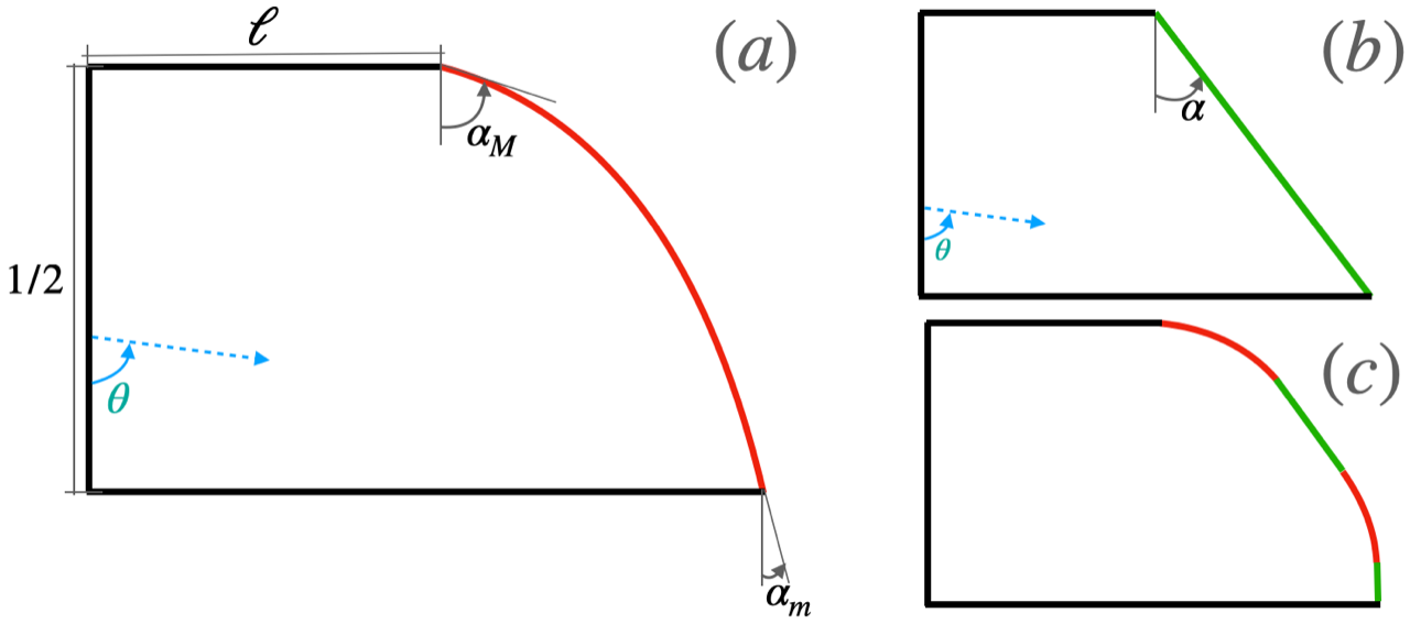
Figure 1: Examples of billiard tables $\Omega$.

In this paper we give rigorous results for the internal-wave billiards in a class of tables which includes the rectangular trapezoid. Specifically, we allow the slanted leg of the trapezoid to be replaced by a piecewise smooth curve with downward concavity; see Fig. 1 for examples of tables in this class and Section 2 for a precise definition of it. Our main result gives a comprehensive description of the asymptotic behavior of all trajectories of the system. In particular, it is proven that there are only three possibilities, with subcases:

• There exist a unique global attractor and a unique global repellor, which are periodic with the same number of bounces off the boundary of the table, and might possibly coincide.

• There exists a beam of periodic trajectories.

  • If the beam is non-degenerate, its boundary consists of two periodic trajectories, which are, respectively, the attractor and the repellor of all trajectories outside of the beam; otherwise

  • the beam may reduce to a single periodic trajectory, which acts as both a global attractor and a global repellor; or

  • the beam may comprise all trajectories, resulting in the case where all trajectories are periodic with the same number of bounces off the boundary.

• All trajectories are dense.

Furthermore, if the slanted side of $\Omega$ does not contain any segment, case (2) coincides with subcase (b); if the slanted side of $\Omega$ is a segment (i.e., $\Omega$ is a rectangular trapezoid), case (2) coincides with subcase (c). All these statements are direct consequences of Theorem 2.2, which describes the dynamics of a suitable Poincaré map for the billiard. Section 2 is devoted to introducing, stating and proving Theorem 2.2.

In Section 3 we study the trapezoidal case in depth, finding in particular that, in parameter space, case (1) has full measure, and case (2) (which is the same as subcase (c) here) and case (3) are non-empty with zero measure. The statement about case (1) is important, we believe, because it is the first mathematical proof — to our knowledge — of the existence of Arnol’d tongues (definition in Section 3) for internal-wave billiards. The statement about case (3) is also interesting, because it explains why this regime was hardly observed in experiments and numerical simulations.

Acknowledgments.

We thank Thierry Dauxois for useful discussions in the early stage of this work and Selim Ghazouani for helping us correct a mistake in an earlier version of this manuscript. The present research was partially supported by the PRIN Grant 2017S35EHN, MUR, Italy. It is also part of the authors’ activity within the UMI Group DinAmicI and the Gruppo Nazionale di Fisica Matematica, INdAM.

2 Reduction to one-dimensional dynamics

We study the internal-wave billiard in a table $\Omega$ that is a generalization of a rectangular trapezoid, like the examples shown in Fig. 1. In suitable units, $\Omega$ has height 1/2 and is completely specified by the position and shape of its rightmost boundary $\partial_{R}\Omega$, which we assume to be the graph of a piecewise $C^{1}$, strictly decreasing, concave function, possibly with the addition of a vertical segment attached to its lower end. Fig. 1(a) defines three important parameters for the dynamics, the angles $\alpha_{m}$, $\alpha_{M}$ and $\theta$. In particular, $\theta\in(0,\pi/2)\cup(\pi/2,\pi)$ is the particle’s initial direction, having assumed (without loss of generality) an initial position on $\partial_{L}\Omega$, the vertical side of $\Omega$. We do not consider horizontal or vertical initial directions for the reasons explained earlier.

If $\theta\in(0,\alpha_{m})\cup(\pi-\alpha_{m},\pi)$, it is easily verified that all reflections at $\partial_{R}\Omega$ are horizontal (as per the definition given in the introduction), implying that every trajectory converges to the lower endpoint of $\partial_{R}\Omega$. If $\theta\in[\alpha_{m},\alpha_{M}]\cup[\pi-\alpha_{M},\pi-\alpha_{m}]$, $\partial_{R}\Omega$ is generally split into two parts, which give rise to horizontal and vertical reflections, respectively. This is the more complicated case, which we do not study at the present time, as we intend to keep our mathematical machinery to a minimum. Moreover, when $\Omega$ is a trapezoid, which a case of interest here, the dynamics for $\theta=\alpha$ is ill-defined.

In this paper we restrict to the case $\theta\in(\alpha_{M},\pi/2)\cup(\pi/2,\pi-\alpha_{M})$ to ensure that all reflections at $\partial_{R}\Omega$ are vertical. Since the particle’s velocity can only assume 4 values, it is convenient to represent the dynamics on $\Omega$ as a linear flow on $\Omega_{4}$, the 4-fold copy of $\Omega$ represented in Fig. 2 as a subset of $\mathbb{R}^{2}$. The linear flow on $\Omega_{4}$ is defined as a fixed-velocity motion on it, with the provision that a trajectory hitting a boundary point continues on the opposite boundary point with the same velocity. Two boundary points of $\Omega_{4}$ are said to be opposite to each other if they belong to the upper/lower boundaries of $\Omega_{4}$ and have the same abscissa, or to the left/right boundaries and have the same ordinate. Fig. 2 also displays a trajectory of the linear flow, together with its projection on $\Omega$. The defining parameter of the linear flow is the angle $\theta$ introduced earlier, which we also call the direction of the flow. We convene that the speed of the flow is 1. It is apparent that the natural projection $\Omega_{4}\longrightarrow\Omega$ maps trajectories of the flow into trajectories of the billiard. The procedure whereby one passes from the internal-wave billiard on $\Omega$ to the linear flow on $\Omega_{4}$ is also called billiard unfolding. (This technique has been applied very fruitfully to polygonal (ordinary) billiards; see, e.g., the reference list of [6].)

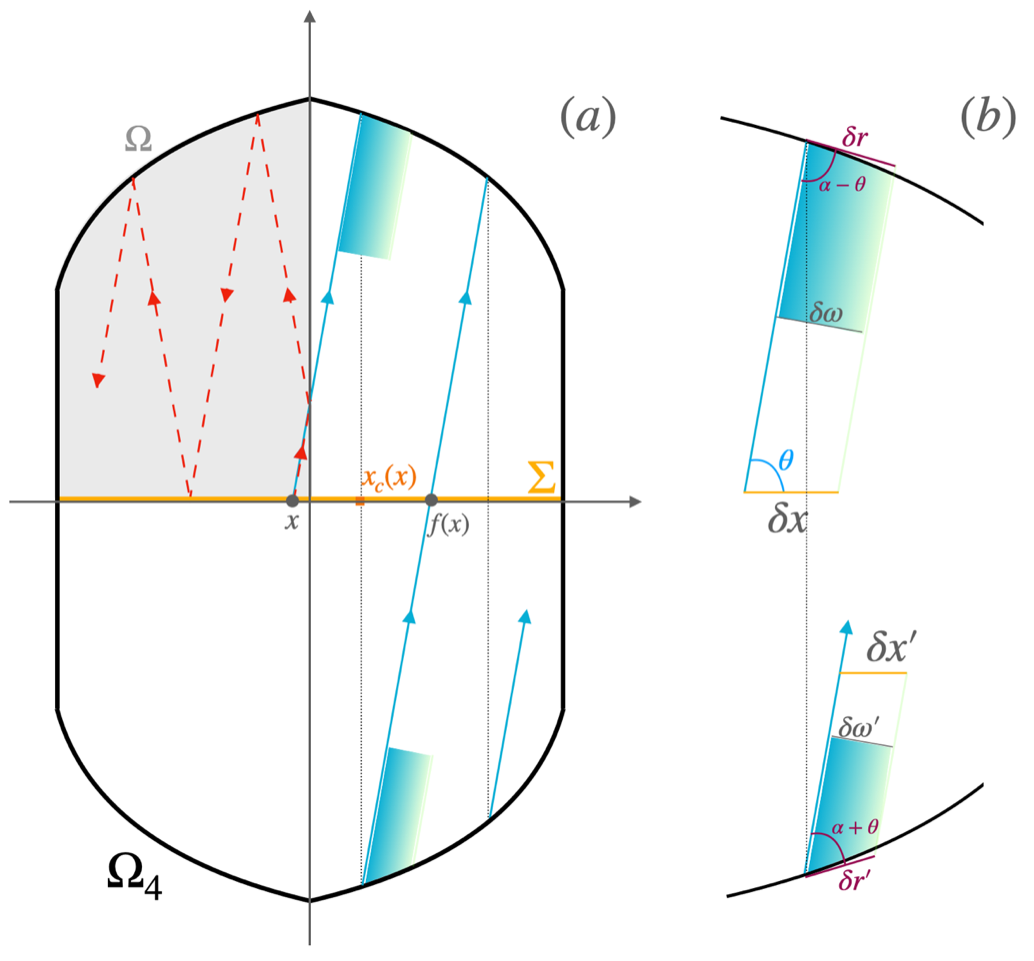
Figure 2: A trajectory of the linear flow in $\Omega_{4}$, together with the corresponding orbit for the Poincaré map $f:\Sigma\longrightarrow\Sigma$. The definition of $x_{c}(x)$, cf. Lemma 2.1, is also illustrated.

Our assumptions on the billiard table $\Omega$, given at the beginning of this section, can be restated as assumptions on $\Omega_{4}$ as follows: the upper boundary of $\Omega_{4}$ is the graph of a function $b:[-1/2,1/2]\longrightarrow\mathbb{R}^{+}$, which is even, piecewise $C^{1}$, concave, and (not necessarily strictly) decreasing on $[0,1/2]$. Set $\alpha(x):=\arctan(b^{\prime}(x))$. This expression fails to be defined in at most countably many points of $(-1/2,1/2)$. The assumptions show that $\alpha$ is a (not necessarily strictly) decreasing odd function with $\alpha(-1/2)=\alpha_{M}$ and $\alpha(1/2)=-\alpha_{M}$. In particular, when $b^{\prime}(x)$ is defined, $x\leq 0$ implies that $\alpha(x)\geq 0$ and $x\geq 0$ implies that $\alpha(x)\leq 0$.

Identifying opposite boundary points of $\Omega_{4}$, which we henceforth do, we regard $\Omega_{4}$ as a surface homeomorphic to a torus. The metric of $\mathbb{R}^{2}$ induces on this surface a metric which is defined and flat everywhere except for a closed curve (which, in topological terms, is a simple, non-contractible loop). The linear flow is the geodesic flow for this metric, subject to a non-isometric identification rule between the two sides of the closed curve.

A convenient way to study the elementary properties of a flow is by means of a suitable Poincaré map. In our case, a good choice is to take the first-return map to the horizontal segment $\Sigma$ shown in Fig. 2(a). We denote it $f:\Sigma\longrightarrow\Sigma$. As per our boundary identifications, $\Sigma$ has the topology of a circle. In any case, with the units that we have chosen, its length is 1. Observe that points on this Poincaré section correspond to the particle being on $\partial_{L}\Omega$ with velocity directed as $\theta$ or $\pi-\theta$. In other words, $\Sigma$ is in 2-to-1 correspondence with the set of initial positions we chose for our dynamics. This fact and the symmetry of $\Omega_{4}$ show that it is no loss of generality to restrict the directions of the linear flow to $\theta\in(\alpha_{M},\pi/2)$. Identifying $\Sigma$ with $\mathbb{S}^{1}:=\mathbb{R}/\mathbb{Z}$ in the natural way, we also regard $f$ as a homeomorphism of $\mathbb{S}^{1}$.

Lemma 2.1

Let us denote by $x_{c}(x)$ the abscissa of the first collision point of the trajectory starting from $x\in\Sigma$ with the upper boundary of $\Omega_{4}$ (see Fig. 2(a)). For all $x\in\Sigma$ such that $\alpha(x_{c}(x))$ is defined, we have

$$f^{\prime}(x)=\frac{\sin(\theta+\alpha(x_{c}(x)))}{\sin(\theta-\alpha(x_{c}(x)))}.$$

Proof. This proof will be illustrated by Fig. 2(b). Given $x\in\Sigma$ such that $\alpha(x_{c}(x))$ is well defined in a neighborhood of $x$, let us take $\delta x$ so small that such neighborhood contains $[x,x+\delta x]$ (having chosen $\delta x>0$ without loss of generality). The beam of (parallel) trajectories stemming from $[x,x+\delta x]$ has width $\delta w=\delta x\sin\theta$ and thus projects on the upper boundary of $\Omega_{4}$ an arc of length

$$\delta r=\frac{\delta w}{\sin(\theta-\alpha)}+o(\delta x)=\delta x\,\frac{\sin\theta}{\sin(\theta-\alpha)}+o(\delta x),\quad\mbox{ as }\delta x\to 0.$$ (2.1)

Here, with a slight abuse of notation, we have denoted $\alpha:=\alpha(x_{c}(x))$. The beam then continues from the opposite arc, on the lower boundary of $\Omega_{4}$. The length of this arc is clearly $\delta r^{\prime}=\delta r$ but, reversing the previous reasoning, its width is $\delta w^{\prime}=\delta r^{\prime}\sin(\theta+\alpha)+o(\delta x)$. The first intersection of this beam with $\Sigma$ is the segment $[f(x),f(x+\delta x)]$, whose length is

$$f(x+\delta x)-f(x)=\frac{\delta w^{\prime}}{\sin\theta}=\delta x\,\frac{\sin(\theta+\alpha)}{\sin(\theta-\alpha)}+o(\delta x),\quad\mbox{ as }\delta x\to 0.$$ (2.2)

Dividing the above by $\delta x$ and taking the limit proves the lemma. Q.E.D.

Another property of $f$ is that, for $x,x_{1}\in\Sigma$,

$$x_{1}=f(x)\quad\Longleftrightarrow\quad-x=f(-x_{1}).$$ (2.3)

In other words, the graph of $f$, as represented in $\mathbb{R}^{2}$, is symmetric around the bisectrix of the second and fourth quadrants. This is easily seen by drawing a first-return segment of a trajectory of the linear flow on $\Omega_{4}$ and rotating $\Omega_{4}$ by 180 degrees, equivalently, by exploiting the fact that the billiard dynamics commutes with time-inversion.

In order to study the topological/combinatorial properties of the internal-wave billiard, it suffices to study the corresponding properties of $f$ on $\mathbb{S}^{1}$. There exists a well-developed theory of circle homeomorphisms, dating back from Poincaré, who introduced the notion of rotation number, which we briefly recall. Let $F:\mathbb{R}\longrightarrow\mathbb{R}$ be a lift of $f$, i.e., a homeomorphism of $\mathbb{R}$ which is well defined on the equivalence classes of $\mathbb{R}/\mathbb{Z}$ (this turns out to be the same as the property $F(x+k)=F(x)+k$, for all $x\in\mathbb{R}$ and $k\in\mathbb{Z}$) and acts like $f$ there. Then the quantity

$$\rho(f):=\lim_{n\to\infty}\frac{F^{n}(x)-x}{n}$$ (2.4)

does not depend on $x$. If taken mod 1, as is customary, it is also independent of the choice of $F$. One calls $\rho(f)$ the rotation number of $f$. In this paper, unless otherwise stated, we represent it as a number in $[0,1)$. Standard references in this area are, e.g., [7, Chap. 1] and [16, §11]. Using only basic results, the next theorem describes the asymptotic behavior of all the orbits of $f$.

Notation.

In what follows we will need to use cyclic indices, namely, elements of $\mathbb{Z}_{q}:=\mathbb{Z}/q\mathbb{Z}$, for some $q\in\mathbb{Z}^{+}$. We can think of them as elements of $\{0,1,\ldots,q-1\}$ with the understanding that the sum of any such element with an integer is intended mod $q$.

Theorem 2.2

Let $\rho(f)\in[0,1)$ denote the rotation number of $f:\mathbb{S}^{1}\longrightarrow\mathbb{S}^{1}$.

• If $\rho(f)\not\in\mathbb{Q}$, $f$ is topologically equivalent (i.e., conjugated via homeomorphism) to the rotation $x\mapsto x+\rho(f)\ (\mathrm{mod}\ 1)$ on $\mathbb{S}^{1}$. In particular, $f$ is minimal, i.e., all orbits are dense.

• If $\rho(f)\in\mathbb{Q}$, we write $\rho(f)=p/q$, where, if $\rho(f)>0$, $p$ and $q$ are coprime positive integers, or else $p=0$ and $q=1$. There exist two sets

  $$\mathcal{P}^{\pm}:=\bigcup_{i=0}^{q-1}\mathcal{P}_{i}^{\pm},$$

  where the $\mathcal{P}_{i}^{\pm}$ are closed intervals. All points in $\mathcal{P}^{\pm}$ are $q$-periodic and such that, for all $i\in\mathbb{Z}_{q}$ and $n\in\mathbb{N}$,

  $$f^{n}\!\left(\mathcal{P}_{i}^{\pm}\right)=\mathcal{P}_{i+pn}^{\pm}.$$

  All points in $\mathbb{S}^{1}\setminus(\mathcal{P}^{+}\cup\mathcal{P}^{-})$ are non-periodic.

  Only two possibilities are given:

  • Each $\mathcal{P}_{i}^{\pm}$ reduces to a point, which we denote $x_{i}^{\pm}$. These points are ordered as follows, according to the orientation of $\mathbb{S}^{1}$:

    $$x_{0}^{-}\leq x_{0}^{+}\leq x_{1}^{-}\leq x_{1}^{+}\leq\cdots\leq x_{q-1}^{-}\leq x_{q-1}^{+}\leq x_{0}^{-}.$$

    So $\mathcal{O}^{\pm}:=\mathcal{P}^{\pm}=\{x_{0}^{\pm},x_{1}^{\pm},\ldots,x_{q-1}^{\pm}\}$ are two (possibly coinciding) periodic orbits such that $f^{n}(x_{i}^{\pm})=x_{i+pn}^{\pm}$, for all $i\in\mathbb{Z}_{q}$ and $n\in\mathbb{N}$. As for the other points:

    $$\forall x\in\left(x_{i}^{-}\,,x_{i}^{+}\right),\qquad f^{n}(x)\in\left(x_{i+pn}^{-}\,,x_{i+pn}^{+}\right)\mbox{ and}$$

    $$\lim_{n\to+\infty}f^{nq}(x)=x_{i}^{+}\,,\quad\lim_{n\to-\infty}f^{nq}(x)=x_{i}^{-}\,;$$

    $$\forall x\in\left(x_{i}^{+}\,,x_{i+1}^{-}\right),\qquad f^{n}(x)\in\left(x_{i+pn}^{+}\,,x_{i+1+pn}^{-}\right)\mbox{ and}$$

    $$\lim_{n\to+\infty}f^{nq}(x)=x_{i}^{+}\,,\quad\lim_{n\to-\infty}f^{nq}(x)=x_{i+1}^{-}\,.$$

    Hence $\mathcal{O}^{+}$, respectively $\mathcal{O}^{-}$, is the global attractor, respectively repellor, of the system.

  • All $\mathcal{P}_{i}^{\pm}$ are non-degenerate intervals, with $\mathcal{P}_{i}^{+}=\mathcal{P}_{i}^{-}$, for all $i\in\mathbb{Z}_{q}$. Denoting any such interval $[x_{i}^{L},x_{i}^{R}]:=\mathcal{P}_{i}^{+}=\mathcal{P}_{i}^{-}$, we have

    $$x_{0}^{L}<x_{0}^{R}\leq x_{1}^{L}<x_{1}^{R}\leq\cdots\leq x_{q-1}^{L}<x_{q-1}^{R}\leq x_{0}^{L},$$

    with the property that $x_{i}^{R}<x_{i+1}^{L}$ holds for some $i\in\mathbb{Z}_{q}$ if, and only if, it holds for all $i\in\mathbb{Z}_{q}$.

    • If $x_{i}^{R}<x_{i+1}^{L}$ for all $i$ then, for all $i\in\mathbb{Z}_{q}$ and $n\in\mathbb{N}$, $f^{n}(\mathcal{P}_{i}^{\pm})=\mathcal{P}_{i+pn}^{\pm}$ and

      $$\forall x\in\left(x_{i}^{R}\,,x_{i+1}^{L}\right),\qquad f^{n}(x)\in\left(x_{i+pn}^{R}\,,x_{i+1+pn}^{L}\right)\mbox{ and}$$

      $$\lim_{n\to+\infty}f^{nq}(x)=x_{i}^{R}\,,\quad\lim_{n\to-\infty}f^{nq}(x)=x_{i+1}^{L}\,.$$

      Therefore $\mathcal{O}^{+}:=\{x_{0}^{R},x_{1}^{R},\ldots,x_{q-1}^{R}\}$ and $\mathcal{O}^{-}:=\{x_{0}^{L},x_{1}^{L},\ldots,x_{q-1}^{L}\}$ are, respectively, the unique (but not global) attractor and repellor of the system.

    • If $x_{i}^{R}=x_{i+1}^{L}$ for all $i$, all orbits are periodic.

  Under the additional assumption that $\partial_{R}\Omega$ does not contain any segment (equivalently, the function $b$ whose graph is the upper boundary of $\Omega_{4}$ is strictly concave), case (b) cannot occur.

Remark 2.3

Since an orbit of $f$ is dense/periodic/attracting/repelling if, and only if, the corresponding flow trajectory in $\Omega_{4}$ is, all the statements of Theorem 2.2 are immediately translated to statements about the internal-wave billiard in $\Omega$. In particular, this proves the claim made in the introduction about the three sole possibilities for the asymptotics of the trajectories.

Proof of Theorem 2.2. Poincaré’s classical theory of circle homeomorphisms [7, Sect. I.1] states that, for any orientation-preserving $f:\mathbb{S}^{1}\longrightarrow\mathbb{S}^{1}$, the following dichotomy holds:

1. If no periodic orbit exists, then $f$ is topologically semiconjugate to an irrational rotation [7, Thm. 1.1], which must necessarily be the rotation by $\rho(f)\not\in\mathbb{Q}$.

2. If a periodic orbit exists and $q$ is its (primitive) period, then necessarily $\rho(f)=p/q$, where $p$ is either 0 or coprime to $q$. Let $x_{0},x_{1},\ldots,x_{q-1}$ be an orientation-preserving labeling of the points of the periodic orbit. By definition of rotation number, for all $i\in\mathbb{Z}_{q}$ and $n\in\mathbb{N}$, one has

   $$f^{n}(x_{i})=x_{i+pn}$$ (2.5)

   (recall the convention on cyclic indices). Therefore

   $$f^{n}\!\left([x_{i},x_{i+1})\right)=[x_{i+pn},x_{i+1+pn}).$$ (2.6)

   Necessarily, then, if $x^{\prime}$ is another periodic point, its combinatorics is the same as that of $x$, that is, its period is $q$ and, for any orientation-preserving labeling $x^{\prime}_{0},x^{\prime}_{1},\ldots,x^{\prime}_{q-1}$ of its orbit, the analogue of (2.5) holds.

To establish (i) it suffices to verify that, for our particular $f$, the topological semiconjugacy of case 1 is in fact a topological conjugacy. This is exactly the assertion of Denjoy’s Theorem for certain circle diffeomorphisms [7, Sect. I.2]. As explained in [7, Rmk on p. 38], Denjoy’s Theorem also holds for homeomorphisms $f$ that are piecewise differentiable and such that $\log|f^{\prime}|$ can be extended to a map with bounded variation. Our $f$ falls in this category, as shown momentarily.

Let us call break point of $f^{\prime}$ any $x\in\mathbb{S}^{1}$ such that

$$\Delta f^{\prime}(x):=\lim_{s\to x^{+}}f^{\prime}(s)-\lim_{s\to x^{-}}f^{\prime}(s)\neq 0,$$ (2.7)

provided the limits exist. A break point $x$ of $f^{\prime}$ is said to be of increase or decrease if $\Delta f^{\prime}(x)>0$ or $\Delta f^{\prime}(x)<0$, respectively.

Lemma 2.4

The homeomorphism $f$ defined earlier is such that $\lim_{s\to x^{\pm}}f^{\prime}(s)$ exists at all $x\in\mathbb{S}^{1}$; $f^{\prime}$ has exactly one break point of increase, denoted $a_{0}$, and at most countably many break points of decrease, denoted $\{a_{i}\}_{i\geq 1}$. This implies that $f^{\prime}$ is continuous on $\mathbb{S}^{1}\setminus\{a_{i}\}_{i\geq 0}$ with positive one-sided limits everywhere. Furthermore, $f$ is concave on the arc $\mathbb{S}^{1}\setminus\{a_{0}\}$. Finally, $\log f^{\prime}$ can be extended to a map with bounded variation.

Proof of Lemma 2.4. By construction of the function $b:\mathbb{S}^{1}\longrightarrow\mathbb{R}^{+}$ introduced earlier, $b^{\prime}$ has exactly one break point of increase $\bar{a}_{0}$ (with $\bar{a}_{0}=-1/2$, in the identification $\mathbb{S}^{1}\cong[-1/2,1/2)$) and at most countably many break points of decrease $\{\bar{a}_{i}\}_{i\geq 1}$. In all other points of $\mathbb{S}^{1}$, $b^{\prime}$ is continuous. Also, $b^{\prime}$ is decreasing (not necessarily strictly) on $\mathbb{S}^{1}\setminus\{\bar{a}_{0}\}$.

On the other hand, Lemma 2.1 states that $f^{\prime}=g_{\theta}\circ\arctan\circ\,b^{\prime}\circ x_{c}$, where

$$g_{\theta}(\alpha):=\frac{\sin(\theta+\alpha)}{\sin(\theta-\alpha)}$$ (2.8)

defines a strictly increasing continuous function $[-\alpha_{M},\alpha_{M}]\longrightarrow\mathbb{R}^{+}$ and $x_{c}:\mathbb{S}^{1}\longrightarrow\mathbb{S}^{1}$ is the map defined in the statement of Lemma 2.1, which is easily seen to be an orientation-preserving homeomorphism. Therefore, there is a bijective correspondence between the break points of $b^{\prime}$ and those of $f^{\prime}$, such that the two functions have the same monotonicity properties between corresponding pairs of break points. This proves all the assertions of Lemma 2.4, except for the last one.

As for the last assertion, let us observe that, by definition, the function $f^{\prime}$ is not defined at its break points, so let us extend it to the whole of $\mathbb{S}^{1}$ by setting $f^{\prime}(a_{i}):=\lim_{s\to a_{i}^{+}}f^{\prime}(s)$ (having employed the common abuse of notation whereby the extension has the same name as the extended function). It is evident that $\mathrm{Var}_{\mathbb{S}^{1}\setminus\{a_{0}\}}(\log f^{\prime})=\Delta\log f^{\prime}(a_{0})$, whence $\mathrm{Var}_{\mathbb{S}^{1}}(\log f^{\prime})=2\,\Delta\log f^{\prime}(a_{0})<\infty$. (Here $\mathrm{Var}_{\mathbb{S}^{1}\setminus\{a_{0}\}}(\cdot)$ is the variation of a real-valued function on the arc $\mathbb{S}^{1}\setminus\{a_{0}\}$ and $\mathrm{Var}_{\mathbb{S}^{1}}(\cdot)$ is the variation on the whole torus, amounting to the former variation plus the variation at $a_{0}$.) Q.E.D.

Now for the statements (ii) of Theorem 2.2. By Poincaré’s dichotomy, if $\rho(f)=p/q$ as in (ii), $f$ has at least a periodic orbit of cardinality $q$, that is, $f^{q}$ has at least $q$ fixed points. The previous proposition and the identity

$$(f^{q})^{\prime}(x)=\prod_{k=0}^{q-1}f^{\prime}(f^{k}(x))$$ (2.9)

show that $(f^{q})^{\prime}$ has at most $q$ break points of increase (namely $\{f^{-k}(a_{0})\}_{k=0}^{q-1}$, keeping in mind that some of these points may coincide), outside of which $f^{q}$ is piecewise $C^{1}$ and concave. For the rest of this proof we refer to this property as the ‘concavity property of $f^{q}$’. Identifying $\mathbb{S}^{1}$ with $[-1/2,1/2)$, the graph of $f^{q}$ can only look like one of the cases depicted in Fig. 3.

Figure 3: Possible graphs of the map $f^{q}$, when a $q$-periodic orbit of $f$ exists.

In particular, the set of fixed points of $f^{q}$ comprises at most $2q$, possibly degenerate, closed intervals $\mathcal{P}_{i}^{\pm}$. By the concavity property of $f^{q}$, the number of such intervals is $2q$ if, and only if, each $\mathcal{P}_{i}^{\pm}$ is a singleton $\{x_{i}^{\pm}\}$. In this case we label $x_{i}^{-}$, respectively, $x_{i}^{+}$, the repelling, respectively, attracting fixed points. Since, relative to the orientation of $\mathbb{S}^{1}$, they alternate, the labelling can be done so that

$$x_{0}^{-}<x_{0}^{+}<x_{1}^{-}<x_{1}^{+}<\cdots<x_{q-1}^{-}<x_{q-1}^{+}<x_{0}^{-}.$$ (2.10)

Thus, by the second part of Poincaré’s dichotomy, $f^{n}(x_{i}^{\pm})=x_{i+pm}^{\pm}$, for all $i\in\mathbb{Z}_{q}$ and $n\in\mathbb{N}$. This the case of Fig. 3(a).

If the graph of $f^{q}$ touches the bisectrix of the first and third quadrants in a single point of abscissa $x$ then, if the graph touches “from below” (Fig. 3(b)), $x$ is a fixed point of $f^{q}$ which is repelling on the left and attracting on the right; if the graph touches “from above” (Fig. 3(c)), $x$ is attracting on the left and repelling on the right. The same must therefore happen for all points of the $f$-periodic orbit $\{f^{i}(x)\}_{i\in\mathbb{Z}_{q}}$, which must be distinct, by part 2 of Poincaré’s dichotomy. The concavity property of $f^{q}$ shows that each of these points must belong to one and only one concave part of $f^{q}$, proving that there can be no other periodic orbits of $f$. Following their orientation on $\mathbb{S}^{1}$, we label $x_{0}^{-},x_{1}^{-},\ldots,x_{q-1}^{-}$ the points of the aforementioned periodic orbit. In the case of left-repelling and right-attracting points (Fig. 3(b)), we also set $x_{i}^{+}:=x_{i}^{-}$; in the case of left-attracting and right-repelling points (Fig. 3(c)), we set $x_{i}^{+}:=x_{i+1}^{-}$. In either case, we finally denote $\mathcal{P}_{i}^{\pm}:=\{x_{i}^{\pm}\}$.

The above considerations prove all the assertions of Theorem 2.2(ii)(a), when the sets $\mathcal{P}_{i}^{\pm}$ are singletons. If $\mathcal{P}^{+}\cup\mathcal{P}^{-}$ is not made up of isolated points, then it must include a closed interval, as we have seen. Take the largest interval (or, in case of a tie, one of the largest intervals) within $\mathcal{P}^{+}\cup\mathcal{P}^{-}$. There can only be two cases: either this closed interval is a proper subset of $\mathbb{S}^{1}$, in which case, without loss of generality, we denote it $\mathcal{P}_{0}^{+}:=[x_{0}^{L},x_{0}^{R}]$; or it is the whole of $\mathbb{S}^{1}$, in which case we choose any point $x_{0}^{L}\in\mathbb{S}^{1}$ and set $x_{0}^{R}:=f(x_{0}^{L})$, $\mathcal{P}_{0}^{+}:=[x_{0}^{L},x_{0}^{R}]$. In the former case, since $f$ is a homeomorphism and preserves the property of being or not an $f^{q}$-periodic point, we see that the sets $\{f^{i}(\mathcal{P}_{0}^{+})\}_{i\in\mathbb{Z}_{q}}$ are pairwise disjoint, closed intervals; they are also distinct, since all $f$-periodic orbits must have period $q$, cf. Fig. 3(d). The concavity property of $f^{q}$ shows that there can be no more periodic points. In the latter case, since the points $\{f^{i}(x_{0}^{L})\}_{i\in\mathbb{Z}_{q}}$ are distinct, we have that the sets $[f^{i}(x_{0}^{L}),f^{i}(x_{0}^{R})]$, $i\in\mathbb{Z}_{q}$, cover $\mathbb{S}^{1}$ and intersect only at their endpoints. See Fig. 3(e).

In either case, we denote $\mathcal{P}_{0}^{+},\mathcal{P}_{1}^{+},\ldots,\mathcal{P}_{q-1}^{+}$ the intervals $\{f^{i}(\mathcal{P}_{0}^{+})\}_{i\in\mathbb{Z}_{q}}$, ordered according to the orientation of $\mathbb{S}^{1}$, and $\mathcal{P}_{i}^{-}:=\mathcal{P}_{i}^{+}$ for all $i$. The above facts prove all the claims of part (ii)(b) of the theorem. In particular, Fig. 3(d) corresponds to case (ii)(b)(1) and Fig. 3(e) corresponds to case (ii)(b)(2).

Lastly, observe that if the function $b$ is strictly concave, (2.9) shows that $f^{q}$ is strictly concave in each of its concavity intervals, whence $\mathcal{P}^{+}\cup\mathcal{P}^{-}$ can only contain isolated points, forcing the case (ii)(a). Q.E.D.

3 The trapezoid

In this section we consider the case where $\Omega$ is the rectangular trapezoid of Fig. 1(b). We improve the general results of Theorem 2.2 and study the sets of parameters for which each of the only possible three cases happens: (1) there exist a global attractor and a global repellor; (2) all orbits are periodic with the same period; (3) all orbits are dense.

We recall that the height of the trapezoid was fixed to 1/2 and that in this case the two equal angles $\alpha_{M}=\alpha_{m}$ are denoted $\alpha$. Let us fix the length of the shorter base to a certain value $\ell>0$ and the direction of the flow to some angle $\theta\in(\alpha,\pi/2)$: this completely determines the homeomorphism $f:\mathbb{S}^{1}\longrightarrow\mathbb{S}^{1}$ introduced in Section 2. Lemma 2.1 shows that the derivative $f^{\prime}$ only takes the values $\Lambda$ and $\Lambda^{-1}$, where

$$\Lambda:=\frac{\sin(\theta+\alpha)}{\sin(\theta-\alpha)}>1.$$ (3.1)

In order to simplify the ensuing computations, we impose the extra condition

$$\theta\geq\arctan(2\ell+\tan\alpha).$$ (3.2)

The left out values of $\theta$ are qualitatively the same as the ones described below. Recalling that the graph of $f$ is symmetric around the bisectrix of the second and fourth quadrants of the square $[-1/2,1/2)^{2}$, we conclude that it must look like the one shown in Fig. 4. More in detail, using the notation of Lemma 2.4, let us call $a_{0}$ and $a_{1}$, respectively, the break points of increase and decrease of $f^{\prime}$. Simple calculations based on Fig. 2 show that

$$a_{0}=\frac{\tan\theta-2\ell}{2\tan\theta}\in\left(0,\frac{1}{2}\right),\qquad a_{1}=-\frac{2\ell+\tan\alpha}{2\tan\theta}\in\left(-\frac{1}{2},0\right),$$ (3.3)

and $f(a_{j})=-a_{j}$, for $j=0,1$.

Figure 4: The graph of $f$ in the case where $\Omega$ is a rectangular trapezoid.

In case our $f$ has a rational rotation number, we can give more precise statements than Theorem 2.2.

Proposition 3.1

Let $f:\mathbb{S}^{1}\longrightarrow\mathbb{S}^{1}$ be as defined above. Assume $\rho(f)=p/q$, with $p,q$ coprime positive integers, or $p=0$, $q=1$. If $q$ is even then $f^{q}=\mathrm{Id}$, that is, all orbits are periodic with primitive period $q$; moreover, $a_{0}$ and $a_{1}$ are in the same periodic orbit. If $q$ is odd then, for any non-degenerate interval $I\subset\mathbb{S}^{1}$, $f^{q}|_{I}\neq\mathrm{Id}|_{I}$; also $a_{0}$ and $a_{1}$ are not in the same periodic orbit.

Proof. We first consider the case where $q$ is even. Let $x_{0}\in\mathbb{S}^{1}$ be a periodic point with (primitive) period $q$ and denote by $x_{0},x_{1},\ldots,x_{q-1}$ the points of its orbit, labeled according to the orientation of $\mathbb{S}^{1}$.

By absurd, we assume that $a_{0}$ and $a_{1}$ are not periodic points. As explained in the proof of Theorem 2.2, in this case $f^{q}$ is piecewise linear with $2q$ break points of $(f^{q})^{\prime}$, which correspond to the points in the backward orbits of $a_{0}$ and $a_{1}$ up to time $-q+1$. In other words, since $a_{0}$ and $a_{1}$ are not periodic points, the graph of $f^{q}$ falls in the case of Fig. 3(a); more precisely, it is a polyline made up of $2q$ segments each of which crosses the bisectrix of the first and third quadrants. So, for all $i\in\mathbb{Z}_{q}$, there are exactly two break points between $x_{i}$ and $x_{i+1}$: one in the orbit of $a_{1}$ and one in the orbit of $a_{0}$ (recall that $i$ is a cyclic index, whence $x_{q}\equiv x_{0}$).

For all points $x\in\mathbb{S}^{1}$ such that $(f^{q})^{\prime}(x)$ exists, we can write $(f^{q})^{\prime}(x)=\Lambda^{n_{+}-n_{-}}$, where $n_{+}=n_{+}(x)$ and $n_{-}=n_{-}(x)$ are the number of times the orbit of $x$ up to time $q-1$ falls in a set where $f^{\prime}$ is $\Lambda$ and $\Lambda^{-1}$, respectively. Clearly, $n_{+}+n_{-}=q$, which is even, so $n_{+}-n_{-}$ is also even. As $x$ varies from $x_{0}$ to $x_{1}$, $(f^{q})^{\prime}(x)$ varies at the two break points in the interval $(x_{0},x_{1})$: it is immediate to verify that passing through the point in the orbit of $a_{0}$ the effect is that $n_{+}$ increases by one and $n_{-}$ decreases by one, and the opposite happens passing through the point in the orbit of $a_{1}$. Therefore, if $(f^{q})^{\prime}(x_{0})\geq\Lambda^{2}$, then $(f^{q})^{\prime}(x)\geq 1$ for all $x\in(x_{0},x_{1}]$ except for two break points. The last two inequalities are in contradiction with $f^{q}(x_{0})=x_{0}$ and $f^{q}(x_{1})=x_{1}$. Analogously, if $(f^{q})^{\prime}(x_{0})\leq\Lambda^{-2}$, then $(f^{q})^{\prime}(x)\leq 1$ for all $x\in[x_{0},x_{1}]$ except for two break points, again a contradiction. Thus, $(f^{q})^{\prime}(x_{0})=1$. But this implies that $(f^{q})^{\prime}(x)=1$ for all $x\in[x_{0},\bar{a})$, where $\bar{a}$ denotes the first break point to the right of $x_{0}$. All such points, then, including $\bar{a}$, are periodic, which is a contradiction, because $\bar{a}$ is in the orbit of $a_{0}$ or $a_{1}$.

We conclude that $a_{0}$ or $a_{1}$ must be periodic points, that is, we are in the cases (b), (c) or (e) of Fig. 3 (case (d) is not achievable with a polyline of $2q$ segments). Let us assume for now that there exist periodic break points of $(f^{q})^{\prime}$, that is, we are not in case (e). Let $x_{0}$ be a periodic break point. One can use essentially the same arguments as in the previous paragraph to prove that $(f^{q})^{\prime}(x_{0}+\varepsilon)=1$ for all small $\varepsilon>0$. (In fact, it is not possible that $x_{0}$ and $x_{1}$ are periodic points, $(f^{q})^{\prime}(x)\geq 1$ for all but one $x$ in $(x_{0},x_{1})$, and $(f^{q})^{\prime}(x_{0}+\varepsilon)>1$ for a small $\varepsilon>0$; the same goes for the analogous statement with reversed inequalities.) But this is incompatible with cases (b) and (c) of Fig. 3.

So only case (e) is possible, i.e., $f^{q}=\mathrm{Id}$. This implies in particular that $a_{0}$ and $a_{1}$ belong to the same periodic orbit. In fact, if not, $(f^{q})^{\prime}$ would have a positive jump at $a_{0}$, contradicting $(f^{q})^{\prime}\equiv 1$.

Finally, let us consider the case where $q$ is odd. In this case $(f^{q})^{\prime}(x)\neq 1$ for all $x$, since there is no choice for $n_{+}$ and $n_{-}$ defined above to satisfy $n_{+}=n_{-}$ and $n_{+}+n_{-}=q$. One also sees that $a_{0}$ and $a_{1}$ are not in the same periodic orbit, otherwise there would be no break points of $(f^{q})^{\prime}$. Q.E.D.

In the rest of the section it will often be convenient to study our homeomorphisms by means of their lifts (cf. Section 2). For a given $f$ as described at the beginning of Section 3, we consider the lift $F:\mathbb{R}\longrightarrow\mathbb{R}$ uniquely defined by the conditions

$$f(x)=F(x)-\left\lfloor F(x)+\frac{1}{2}\right\rfloor,\quad\forall x\in\left[-\frac{1}{2},\frac{1}{2}\right);$$ (3.4)

$$F(a_{1})=-a_{1}.$$ (3.5)

This implies in particular that $F(a_{0})=1-a_{0}$ (recall that $f(a_{j})=-a_{j}$). The last two equalities, together with the knowledge of the slope of $F$ before and after $a_{0}$ and $a_{1}$, cf. (3.1), allow one to derive an expression for $F$:

$$F(x)=\left\{\begin{array}[]{ll}\displaystyle-a_{1}+\Lambda^{-1}(x-a_{1}),&\text{if }x\in[a_{1},a_{0}];\\[4.0pt] 1-a_{0}+\Lambda(x-a_{0}),&\text{if }x\in[a_{0},a_{1}+1];\\[4.0pt] F(x+k)-k,&\text{if }x+k\in[a_{1},a_{1}+1]\text{ with }k\in\mathbb{Z}.\end{array}\right.$$ (3.6)

An example of $F$ is shown in Fig. 5.

Figure 5: Graph of the lift $F$ corresponding to the map of Fig. 4. The short dashed lines have equations $y=-x$, $y=-x+1$ and $y=-x+2$ in coordinates $(x,y)$.

The main result of this part of the paper is that the typical $f$ for a trapezoidal billiard has a rational rotation number. Here ‘typical’ is intended in the strongest sense, that of measure theory.

Theorem 3.2

Let $f_{\ell,\alpha,\theta}:\mathbb{S}^{1}\longrightarrow\mathbb{S}^{1}$ be the map introduced earlier, for a given choice of the parameters $\ell>0$, $0<\alpha<\theta<\pi/2$. Then, for every $\ell$ and Lebesgue-a.e. $(\alpha,\theta)$,

$$\rho(f_{\ell,\alpha,\theta})\in\mathbb{Q}.$$

The proof of this theorem, which uses more sophisticated techniques than the rest of the paper, is postponed to Appendix A.

A finer analysis of the properties of $\rho(f)$, as $f$ varies, comes from considering one-parameter families of maps. More specifically, we assume to be given a continuous strictly increasing family $(f_{u})_{u\in[u_{1},u_{2}]}$ of homeomorphisms of our type. This means that, for every $u\in[u_{1},u_{2}]$, there exists a lift $F_{u}$ of $f_{u}$ such that the family $(F_{u})$ has the following properties:

• $u\mapsto F_{u}$ is continuous in the sup norm of $\mathbb{R}$;

• for all $x\in\mathbb{R}$, $u\mapsto F_{u}(x)$ is strictly increasing;

cf. [16, §11.1]. A quick look at Fig. 5 convinces one that a family of circle homeomorphisms in our class is continuous and strictly increasing if, and only if, the coordinates of the two break points $a_{j}$ of $f^{\prime}_{u}$ are continuous and strictly decreasing functions of $u$ (observe that the corner points of $F_{u}$ are constrained to lie on the lines $y=-x+k$, with $k\in\mathbb{Z}$). For example, employing again the notation $f_{\ell,\alpha,\theta}$, it follows from (3.3) that

$$(f_{\ell,\alpha,\theta})_{\ell\in[\ell_{1},\ell_{2}]},\qquad(f_{\ell,\alpha,-\theta})_{\theta\in[\theta_{1},\theta_{2}]},\qquad(f_{u,\kappa u,\theta})_{u\in[u_{1},u_{2}]},$$ (3.7)

with $\kappa>0$, are continuous strictly increasing families whenever they are defined.

Theorem 3.3

Let $(f_{u})_{u\in[u_{1},u_{2}]}$ be a continuous strictly increasing family of circle homeomorphism of the type $f_{\ell,\alpha,\theta}$, with $\rho_{1}:=\rho(f_{u_{1}})<\rho_{2}:=\rho(f_{u_{2}})$. Here $\rho(f_{u})$ is intended as the actual r.h.s. of (2.4) with $F=F_{u}$; in other words, $\rho(f_{u})$ can take all real values. Then the function

$$\rho:[u_{1},u_{2}]\longrightarrow\mathbb{R},\quad\rho(u):=\rho(f_{u}),$$

is an increasing devil’s staircase (namely, an increasing, continuous, non-constant function that is constant on each interval of a family with dense union). This implies in particular that each rotation number in $[\rho_{1},\rho_{2}]$ is realized by at least one $f_{u}$. Moreover, $\rho$ is constant on an interval if, and only if, the constant is 0 or $p/q$, with $p,q$ coprime integers and $q$ odd.

Proof. It is a known fact that the function $f\mapsto\rho(f)$ is continuous and increasing in the space of orientation-preserving circle homeomorphisms. This means that the r.h.s. of (2.4), as an element of $\mathbb{R}$, is a continuous function of $F$, w.r.t the sup norm, which does not decrease if $F$ is increased pointwise; more details in [16, §11.1]. Hence, $u\mapsto\rho(u)$ is continuous and increasing. Moreover, by general results (see, e.g., [16, Prop. 11.1.9]), it is strictly increasing at irrational values, i.e., if $\rho(u)\not\in\mathbb{Q}$ then, for all sufficiently close $u_{-}<u<u_{+}$, $\rho(u_{-})<\rho(u)<\rho(u_{+})$.

The next proposition is a corollary of Proposition 3.1. We will use it to prove Theorem 3.3, but the results are of independent interest as well.

Proposition 3.4

Denote by $Q_{o}$ the set of all rationals that can be written as $p/q$, with $p$ and $q$ coprime and $q$ odd (by convention, $0=0/1\in Q_{o}$). Then:

• for all $r\in Q_{o}$, $\rho^{-1}(r)$ is a non-degenerate closed interval and, for all $u\in\rho^{-1}(r)$, $f_{u}$ is not topologically equivalent to a rotation;

• for all $r\in\mathbb{R}\setminus Q_{o}$, $\rho^{-1}(r)$ is a point $u_{r}$ and $f_{u_{r}}$ is topologically equivalent to the rotation by $\rho(f_{u_{r}})$.

Proof of Proposition 3.4. Let us first observe that, since $F_{u}(x)$ is strictly increasing both in $u$ and $x$, the graphs of $F_{u}^{q}$ are strictly increasing in $u$, for all $q\in\mathbb{Z}^{+}$, i.e., $(f_{u}^{q})_{u\in[u_{1},u_{2}]}$ is also a strictly increasing continuous family of circle homeomorphisms.

If, for a given $u_{r}$, $\rho(f_{u_{r}})=r\in Q_{o}$, Proposition 3.1 shows that $f_{u_{r}}$ falls in the case (ii)(a) of Theorem 2.2 and so it cannot be conjugate to a rotation (an attractor exists). Moreover, by the continuity of $(f_{u}^{q})_{u}$, a left and/or right perturbation in $u$ preserves the $q$ intersections between the graph of $f_{u}^{q}$ and the bisectrix of the first and third quadrants in $[-1/2,1/2)^{2}$. So, for such $u$, $\rho(f_{u})=r$. This ends the proof of part (i).

As for part (ii), we first consider $r\in\mathbb{Q}\setminus Q_{o}$ and then $r\in\mathbb{R}\setminus\mathbb{Q}$. If $\rho(f_{u})=r\in\mathbb{Q}\setminus Q_{o}$, Proposition 3.1 gives $f_{u}^{q}=\mathrm{Id}$. By the strict monotonicity and $u$-continuity of $f_{u}^{q}$, any arbitrarily small perturbation in $u$ will produce a positive distance between the graph of $f_{u}^{q}$ and the bisectrix of the first and third quadrants, making $\rho(f_{u})$ arbitrarily close to an integer $p$, but unequal to $p$. Since it is a general fact that $\rho(f^{q})=q\rho(f)$ mod 1, it follows that $\rho(f_{u})$ must vary, whence $\rho^{-1}(r)=\{u_{r}\}$. Moreover, it is a general fact that if $f^{q}=\mathrm{Id}$ then $f$ is topologically equivalent to the rotation by $p/q$, for some $p$. (Here is a sketch of its proof. By Poincaré duality, $\rho(f)=p/q$, with $p$ coprime to $q$. Given a periodic orbit $\{x_{0},x_{1},\cdots,x_{q-1}\}$, labeled according to the orientation of $\mathbb{S}^{1}$, one defines $\phi|_{[x_{0},x_{1}]}$ to be any orientation-preserving homeomorphism $[x_{0},x_{1}]\longrightarrow[0,1/q]$. Then, for $x\in[x_{i},x_{i+1}]$, $i\in\mathbb{Z}_{q}$, one chooses $n$ such that $np=i$ mod $q$ and defines $\phi(x):=\phi(f^{-np}(x))+i/q$. This gives a homeomorphism $[x_{i},x_{i+1}]\longrightarrow[i/q,(i+1)/q]$. It is easy to verify that, for $r\in[0,1)$, $\phi\circ f\circ\phi^{-1}(r)=r+p/q$ mod 1.)

Finally, if $\rho(f_{u_{r}})=r\in\mathbb{R}\setminus\mathbb{Q}$, the fact that $\rho^{-1}(r)=\{u_{r}\}$ follows from the strict monotonicity of $\rho$ at irrational values, as recalled earlier, and the fact that $f_{u_{r}}$ is topologically equivalent to the corresponding rotation follows from Theorem 2.2(i). Q.E.D.

A standard result of the theory of rotation numbers, cf. [16, Prop. 11.1.11], states that, if $(f_{u})_{u\in[u_{1},u_{2}]}$ is a continuous monotonic family of orientation-preserving circle homeomorphisms such that $\rho(f_{u})$ is non-constant, and there exists a dense $S\subset\mathbb{Q}$ such that, whenever $\rho(f_{u})\in S$, $f_{u}$ is not topologically equivalent to a rotation, then $u\mapsto\rho(f_{u})$ is a devil’s staircase. We apply this result with $S:=Q_{o}$ as in the statement of Proposition 3.4. This is obviously a dense subset of the rationals. Since $\rho$ is non-constant by assumption, we conclude that $\rho$ is a devil’s staircase, whose claimed properties have been proved earlier. This ends the proof of Theorem 3.3. Q.E.D.

We give some final comments on the significance of the above results for the dynamics of internal-wave billiards in rectangular trapezoids.

The set of all rectangular trapezoids has 3 degrees of freedom, so the set of all internal-wave billiard flows with unit speed in a rectangular trapezoid has 4 degrees of freedom. On the other hand, as for all billiard dynamics, a rescaling of the table gives rise to the same flow up to a rescaling of time. Moreover, an internal-wave billiard has another symmetry: a vertical or horizontal dilation of the table also leads to the same flow up to a rescaling of time. So the effective degrees of freedom in this problem are 2. We can choose to fix $\ell>0$ and represent the set of all flows as the parameter space $\mathcal{T}:=\left\{(\alpha,\theta)\>\left|\>0<\alpha<\theta<\pi/2\right.\!\right\}$.

Our results prove a few facts that were already observed, to a larger or smaller extent, in the physical literature:

1. The parameter space is made up almost entirely by Arnol’d tongues. An Arnol’d tongue is the set of parameters for which the rotation number of the Poincaré map $f$ assumes a given rational value, provided it has positive measure in parameter space. Theorem 3.2 implies that almost every $(\alpha,\theta)\in\mathcal{T}$ is part of a tongue. Theorem 3.3, applied to all families $(f_{\ell,\alpha,-\theta})_{\theta\in(-\pi/2,-\alpha)}$, for $\alpha\in(0,\pi/2)$, shows that only rotation numbers with odd denominators (in simplest terms) possess a tongue. This was already observed in [19]. In view of Proposition 3.1, the above result proves that, for almost all choices of the parameters, the billiard flow has a global attractor and a global repellor.

2. The set of parameters $(\alpha,\theta)$ for which all trajectories are part of the same periodic beam is given by a countable number of smooth curves in $\mathcal{T}$. In fact, Proposition 3.1 shows that this case occurs if, and only if, $\rho(f)=p/q$, with $q$ even (as a reduced fraction). It also shows that such condition is equivalent to

   $$F_{\ell,\alpha,\theta}^{q}(a_{0})=a_{0}+p,$$ (3.8)

   where $F_{\ell,\alpha,\theta}$ is the lift of $f=f_{\ell,\alpha,\theta}$. By way of (3.3) and (3.6), equation (3.8) is turned into a finite number of disjoint quadratic equations in the variables $\ell$, $\tan\alpha,\tan\theta$.

3. The set of parameters $(\alpha,\theta)$ for which all trajectories are dense is a zero-measure Cantor set, where a Cantor set is an uncountable set with no interior points. The nullity of the measure is a consequence of Theorem 3.2. The Cantor property comes from the proof of Theorem 3.3, applied to the same families as in point 1: for all $\alpha$, no interval in the parameter $\theta$ may correspond only to irrational rotation numbers.

4. All rotation numbers in $[0,1)$ — or, if we think of rotation numbers as taking values in the whole of $\mathbb{R}$, all rotation numbers in $\mathbb{R}^{+}$ — are realized. In fact, it is easy to see that $F_{\ell,\alpha,\theta}$ converges to the identity, as $\theta\to\pi/2^{-}$, for all $\alpha$; whereas, for $\theta\to 0^{+}$, $F_{\ell,\theta/2,\theta}\approx T_{\Delta}$, where $T_{\Delta}:\mathbb{R}\longrightarrow\mathbb{R}$ is the translation by $\Delta:=2\ell/\tan\theta$ (all convergences are in the sup norm of $\mathbb{R}$). With reference to point 1 above, this proves in particular that all rotation numbers with odd denominators (in simplest terms) possess Arnol’d tongues in $\mathcal{T}$.

Remark 3.5

The trapezoidal billiards considered in [19] depend on two parameters, $d$ and $\tau$, where $\tau>0$ is the height of the trapezoid (in our case it is 1/2) and $d\in(-1,1)$ is such that the shorter base is $1+d$ (in our case it is $\ell$). In keeping with the fact that two parameters are enough to describe all internal-billiard flows, Maas et al choose to fix the longer base of the trapezoid to be 2 and $\theta=\pi/4$. The return map $\tilde{f}$ they use is then defined on $\tilde{\Sigma}=[-\tau,\tau)$. It follows that $\tilde{f}=\phi\circ f\circ\phi^{-1}$, where $\phi:[-1/2,1/2)\longrightarrow[-\tau,\tau)$ is given by $\phi(x)=2\tau x$ and $f$ is the map of Section 3 with parameters

$$\ell=1+d,\qquad\alpha=\arctan(2(1-d)),\qquad\theta=\arctan(2\tau).$$ (3.9)

All results we prove for $f$ hold for $\tilde{f}$ with the corresponding parameters. In Fig. 6 we draw some Arnol’d tongues, computed rigorously with our methods, over the figure [19, Fig. 2], which describes simulations by Maas et al. More in detail, for some pairs $(p,q)$ of coprime integers, same-colored curves in Fig. 6 represent the boundary of the region in $(d,\tau)$-space where the rotation number equals $p/q$. The curves are computed as follows. The proof of Theorem 3.3 shows that the boundary of the mentioned region corresponds to the case where $a_{0}$ or $a_{1}$ are periodic orbits with rotation number $p/q$. These two occurrences are respectively equivalent to the two equations

$$F^{q}(a_{j})=a_{j}+p,\qquad j=0,1.$$ (3.10)

Proposition 3.1 states that the two occurrences, and thus the two equations, are distinct when $q$ is odd and the same when $q$ is even. As seen in point 2 above, each equation amounts to a finite number of disjoint equations in $\ell,\alpha,\theta$, which are then turned into disjoint equations in $d,\tau$ via (3.9). For example, in the case $(p,q)=(2,3)$, the lower and upper boundaries of the tongue are given respectively by

$$\tau=\frac{1}{4}\!\left(d+5+\sqrt{9d^{2}+10d+17}\right),\qquad\tau=\frac{1}{2}\!\left(d+2+\sqrt{d^{2}+8}\right).$$ (3.11)

In the case $(p,q)=(1,4)$, to give an example with even denominator, the tongue degenerates to a single curve of equation

$$\tau=d+3+2\sqrt{2+2d}.$$ (3.12)

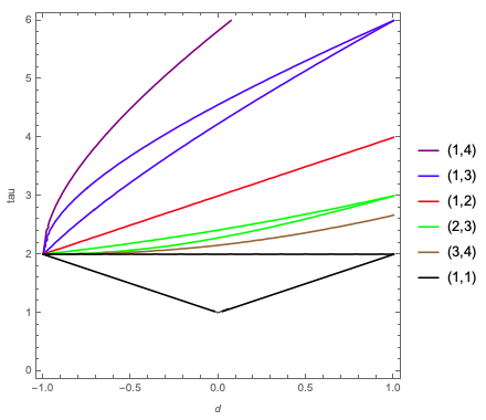
Figure 6: Arnol’d tongues in $(d,\tau)$-space. The figure shows the boundaries of some tongues relative to rotation numbers $p/q$, with $q$ odd, represented as curves of the same color. For $q$ even, each tongue degenerates to a single curve. The label of a tongue or a curve is the pair $(p,q)$. Compare with Fig. 2 of [19].

Appendix A Appendix: Piecewise linear circle homeomorphisms with two break points and dilation surfaces

In this appendix we prove Theorem 3.2 by mapping our problem into an analogous problem in the context of dilation surfaces [8, 2, 9]. Our arguments will be adaptations of arguments found in [2]. For this reason, and also to avoid a very cumbersome appendix, we will not give every last detail of each proof, referring the reader to the explanations of [2].

Figure 7: Dilation surface $\Omega^{\prime}\equiv\Omega^{\prime}_{m}$, with $m\in[1/2,1)$. The gray vertical sides, of length 1, are identified by means of a translation. The blue sides, of lengths $m$ and $1-m$ respectively, are identified by means of an affine transformation. Same for the red sides. Points marked with the same symbol are identified and represent a singular point of $\Omega^{\prime}$. The curve $\Sigma^{\prime}$, a topological circle, is the bottom side of the square.

The central idea is to view our maps $f_{\ell,\alpha,\theta}$ as first-return maps for the linear flow on the dilation surface $\Omega^{\prime}$ illustrated in Fig. 7; see caption for a complete definition of $\Omega^{\prime}\equiv\Omega^{\prime}_{m}$, for $m\in[1/2,1)$. More in detail, in view of Fig. 7, consider the flow on $\Omega^{\prime}$ defined by the constant vector field of direction $\psi\in(0,\pi/2]$. We refer to it as the linear flow of direction $\psi$. The curve $\Sigma^{\prime}$ has the topology of a circle and is clearly a cross-section for the linear flow. We call $g_{m,\psi}:\Sigma^{\prime}\longrightarrow\Sigma^{\prime}$ the corresponding Poincaré map, where $m\in[1/2,1)$ is the parameter indicated in Fig. 7.

Now, to the triple of parameters $(\ell,\alpha,\theta)$, with $\ell>0$ and $0<\alpha<\theta\leq\pi/2$, we associate the pair $(m,\psi)\in[1/2,1)\times(0,\pi/2]$ with

$$m:=\frac{1}{2}+\frac{\tan\alpha}{2\tan\theta},\qquad\psi:=\arctan\left[\left(\frac{2\ell}{\tan\theta}+m-1\right)^{-1}\right].$$ (A.1)

We claim that, up to conjugation, $g_{m,\psi}$ acts on $\Sigma^{\prime}$ as $f_{\ell,\alpha,\theta}$ acts on $\Sigma$. First observe that, by (A.1) and (3.3), $m=a_{0}-a_{1}$. This is actually the reason behind the definition of $m$. Also, cf. (3.1) and Fig. 4,

$$\Lambda=\frac{a_{0}-a_{1}}{1-a_{0}+a_{1}}=\frac{m}{1-m}.$$ (A.2)

Redrawing Fig. 2 for the case where $\Omega_{4}$ is a hexagon (corresponding to $\Omega$ being our rectangular trapezoid) shows that, up to a rotation of $\Sigma$, the action of $f_{\ell,\alpha,\theta}$ is completely determined by the fact that an arc of length $1-m$ (the arc $[a_{0},a_{1}]$ in Fig. 4) is uniformly expanded by a factor $\Lambda=m/(1-m)$ and its left endpoint is moved to the right by quantity $2\ell/\tan\theta$ (here left and right are relative to the orientation of $\Sigma$). The complementary arc, of length $m$, follows suit: it is uniformly contracted by a factor $\Lambda^{-1}$ and its left endpoint is moved to the right by a quantity $(2\ell+\tan\alpha)/\tan\theta$. On the other hand, by construction, $g_{m,\psi}$ uniformly expands an arc of length $1-m$ by a factor $m/(1-m)=\Lambda$ and moves its left endpoint to the right by a quantity $1/\tan\psi+1-m$. Again, the complementary arc, of length $m$, follows suit: it is uniformly contracted by a factor $\Lambda^{-1}$ and its left endpoint is moved to the right by a quantity $1/\tan\psi+m$. So, for any isometric identification $\Sigma\cong\Sigma^{\prime}$, $f_{\ell,\alpha,\theta}$ coincides with $g_{m,\psi}$ up to a conjugation by rotation if, and only if,

$$\frac{2\ell}{\tan\theta}=\frac{1}{\tan\psi}+1-m,$$ (A.3)

which is exactly the second relation of (A.1).

In the remainder, we will simplify the notation by introducing the new parameter

$$s:=\frac{1}{\tan\psi}=\frac{2\ell}{\tan\theta}+m-1=\frac{4\ell+\tan\alpha}{2\tan\theta}-\frac{1}{2}$$ (A.4)

and rewriting $g_{s}:=g_{m,\psi}:\mathbb{S}^{1}\longrightarrow\mathbb{S}^{1}$ (via the natural identification $\Sigma^{\prime}\cong\mathbb{S}^{1}$). The latter change of notation is convenient because we are interested in fixing $\ell,m$ and varying $s$. The main goal of this appendix is to show that the rotation number of $g_{s}$ is irrational for a.e. $s$.

Theorem A.1

For all $m\in[1/2,1)$ and Lebesgue-a.e. $s\in[0,+\infty)$, $\rho(g_{s})\in\mathbb{Q}$.

Proof. Here is where non-trivial geometric tools for dilation surfaces come into play. We will see that it is useful to consider the action that the group of orientation-preserving affine diffeomorphisms of $\Omega^{\prime}$ has on the directional foliations of that surface. A directional foliation of $\Omega^{\prime}$ is simply the collection of all the trajectories of a given linear flow on $\Omega^{\prime}$. For such an action, obviously, the translational part of an affine diffeomorphism is irrelevant, as is any scaling factor in the linear part. In other words, the relevant information is stored in $V_{\Omega^{\prime}}$, the Veech group of $\Omega^{\prime}$, which is defined to be the group of the linear parts of all orientation-preserving affine diffeomorphisms of $\Omega^{\prime}$, modulo multiplicative factors. Having chosen a reference system for $\Omega^{\prime}$ (in the present case, the one implicit in Fig. 7), $V_{\Omega^{\prime}}$ is regarded as a subgroup of $SL(2,\mathbb{R})$.

It turns out, cf. [2, Thm. 4], that $V_{\Omega^{\prime}}$ is the group generated by the matrices

$$A=\begin{pmatrix}1&1\\ 0&1\end{pmatrix},\qquad B=\begin{pmatrix}1&0\\ 1/(m-m^{2})&1\end{pmatrix},\qquad-I=\begin{pmatrix}-1&0\\ 0&-1\end{pmatrix}.$$ (A.5)

In the interest of an accessible exposition we show, by means of Figs 8 and 9, that $A,B\in V_{\Omega^{\prime}}$ (the fact that $-I\in V_{\Omega^{\prime}}$ is obvious). We do not prove, however, that the group generated by $A,B,-I$ is the entire Veech group, because the forthcoming arguments work as well if one replaces $V_{\Omega^{\prime}}$ with $\langle A,B,-I\rangle$.

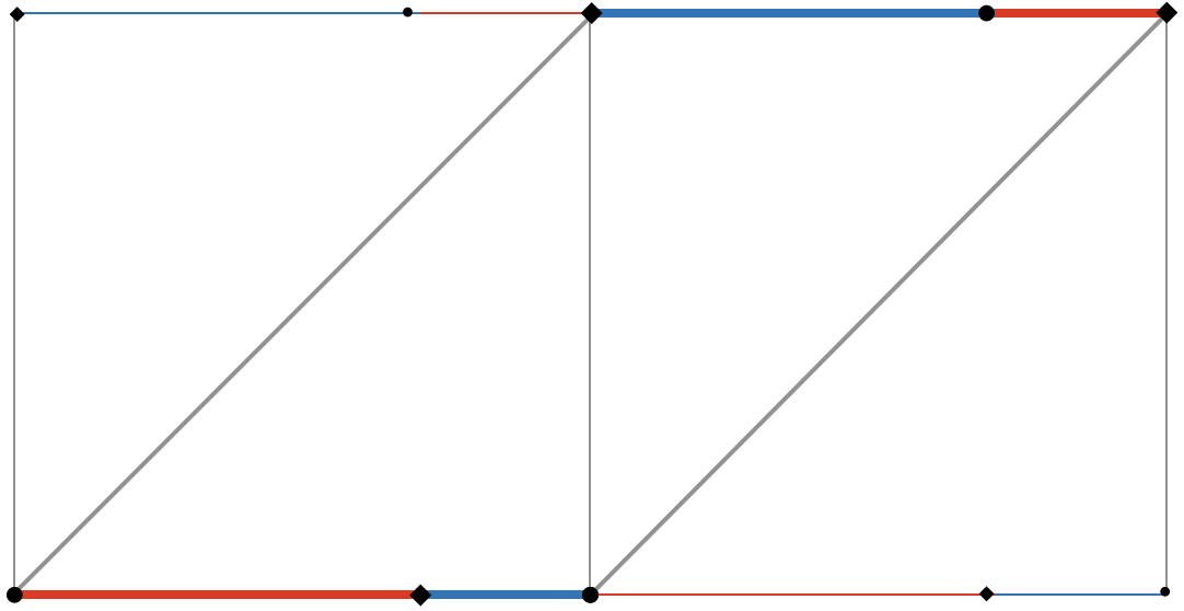
Figure 8: The action of $A$ on $\Omega^{\prime}$. More precisely, by way of a two-fold cover of $\Omega^{\prime}$, the figure shows the action of an orientation-preserving affine diffeomorphism of $\Omega^{\prime}$ whose linear part is $A$.

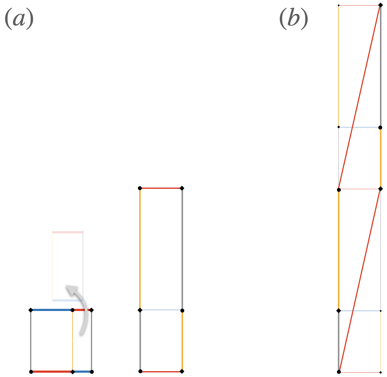
Figure 9: The action of $B$ on $\Omega^{\prime}$. As in Fig. 8, part (b) shows the action of an orientation-preserving affine diffeomorphism of $\Omega^{\prime}$ whose linear part is $B$, but here we are using another planar representation of $\Omega^{\prime}$, constructed in part (a).

We parametrize the directional foliations by means of the variable $s=1/\tan\psi$, where we extend the domain of $\psi$ to $[0,\pi)$. This means that we regard $s$ as a projective variable in $\mathbb{R}P^{1}\cong\mathbb{R}\cup\{\infty\}$. Notice that, in so doing, we are only considering directional foliations with a non-negative vertical component or, more truthfully, we are considering foliations up to their orientation. To see how an element

$$M=\begin{pmatrix}a&b\\ c&d\end{pmatrix}$$ (A.6)

of $V_{\Omega^{\prime}}$ acts on the foliation parametrized by $s$, consider a vector $v=(r,r\tan\psi)=(r,r/s)$, $r\in\mathbb{R}\setminus\{0\}$, in the direction of such foliation (modulo orientation). In the coordinate $s$, the action of $M$ is clearly

$$s=\frac{r}{r/s}\mapsto\frac{ar+b(r/s)}{cr+d(r/s)}=\frac{as+b}{cs+d}.$$ (A.7)

With a slight abuse of notation, we denote the above r.h.s. by $M(s)\in\mathbb{R}P^{1}$. Obviously, $s\mapsto M(s)$ is the Möbius transformation given by the matrix $M$, regarded as an element of $PSL(2,\mathbb{R})$ (with the standard abuse).

We call $\Gamma_{\Omega^{\prime}}$ the projection of $V_{\Omega^{\prime}}$ into $PSL(2,\mathbb{R})$. Thus, $\Gamma_{\Omega^{\prime}}$ is the Fuchsian group generated by $A$ and $B$. In this spirit, for $M\in\Gamma_{\Omega^{\prime}}$, we extend the definition of $M(z):=(az+b)/(cz+d)$ to $z\in\mathbb{H}$, the hyperbolic upper half plane. In this way, $\Gamma_{\Omega^{\prime}}$ acts on $\mathbb{H}$, so its action on $\mathbb{R}P^{1}$ can be studied as its action on the “boundary at infinity” of $\mathbb{H}$.

It is shown in [2, §3.3] that the maximal set of $\mathbb{R}P^{1}$ where the action of $\Gamma_{\Omega^{\prime}}$ is properly discontinuous is a set $D_{\Gamma}$ of full Lebesgue measure and that $D_{\Gamma}/\Gamma_{\Omega^{\prime}}$ has the topology of a circle. A corresponding fundamental domain $J_{\Gamma}$ can be found by taking the “boundary at infinity” of a fundamental domain $\mathcal{F}_{\Gamma}$ for the action of $\Gamma_{\Omega^{\prime}}$ on $\mathbb{H}$. An example of $\mathcal{F}_{\Gamma}$, calculated by means of $A$ and $B$, is depicted in Fig. 10, together with its corresponding

$$J_{\Gamma}=\left[\frac{1}{-2+1/(m-m^{2})}\,,\,\frac{1}{2}\right].$$ (A.8)

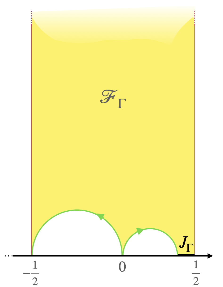
Figure 10: The fundamental domains $\mathcal{F}_{\Gamma}$ and $J_{\Gamma}$.

Lemma A.2

Every map $g_{s}$ with $s\in J_{\Gamma}$ has a fixed point.

Proof of Lemma A.2. The statement is true for a larger interval of directions, namely, $[1-m,m]\supset J_{\Gamma}$. In fact, as in Fig. 11, one can draw the cone of half-lines that homothetically projects that upper red segment into the lower red segment of $\Omega^{\prime}$. The directions defined by this cone, in the projective coordinate $s$, are exactly $[1-m,m]$. It is easily seen that the intersection of every half-line of the cone with $\Omega^{\prime}$ is a closed trajectory for the linear flow defined by the corresponding direction $s$, with the property that the trajectory closes up at the first return to $\Sigma^{\prime}$. In other words, the trajectory corresponds to a fixed point of $g_{s}$. Q.E.D.

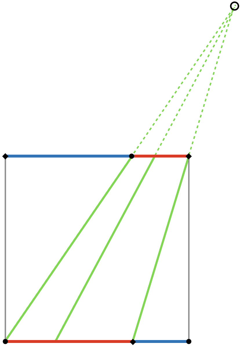
Figure 11: Closed leaves for $s\in[1-m,m]$.

Lemma A.3

For $s\in\mathbb{R}P^{1}$ and $M\in\Gamma_{\Omega^{\prime}}$, $g_{s}$ has a periodic orbit if, and only if, $g_{M(s)}$ has a periodic orbit.

Proof of Lemma A.3. The proof is immediate: $g_{s}$ has a periodic orbit if, and only, if the foliation labeled by $s$ has a closed leaf. Now, $M\in\Gamma_{\Omega^{\prime}}$ means that there exists an orientation-preserving affine diffeomorphism $\tau_{M}$ of $\Omega^{\prime}$ whose linear part, up to factors, is $M$. By definition of $M(s)$, cf. (A.7), $\tau_{M}$ transform the foliation labeled by $s$ into the foliation labeled by $M(s)$ and the closed leaf for the former into a closed leaf for the latter, and viceversa. Q.E.D.

We are now in a position to quickly finish the proof of Theorem A.1. By Poincaré’s classical theory (see proof of Theorem 2.2), $\rho(g_{s})\in\mathbb{Q}$ if, and only, if $g_{s}$ has a periodic orbit. The previous statements imply that, for every $s\in D_{\Gamma}$, there exists an $M\in\Gamma_{\Omega^{\prime}}$ such that $M(s)\in J_{\Gamma}$. By Lemmas A.2 and A.3, $\rho(g_{s})\in\mathbb{Q}$. Restricting $s$ to $D_{\Gamma}\cap[0,+\infty)$ yields the theorem. Q.E.D.

Proof of Theorem 3.2. Take $\ell>0$ constant. Fixing $m\in[1/2,1)$ means fixing the ratio $\tan\alpha/\tan\theta=2m-1\in[0,1)$, cf. the first relation of (A.1). By (A.4), an almost sure property in terms of $s$ translates in an almost sure property in terms of $\tan\theta$. So, in every half-line of the strip

$$\left(\tan\theta,\frac{\tan\alpha}{\tan\theta}\right)\in(0,+\infty)\times[0,1),$$ (A.9)

the property $\rho(f_{\ell,\alpha,\theta})\in\mathbb{Q}$ occurs Lebesgue-almost everywhere. Since the transformation $(\alpha,\theta)\mapsto(\tan\theta,\tan\alpha/\tan\theta)$ has positive Jacobian, the same property holds Lebesgue-almost everywhere in the triangle $\mathcal{T}:=\left\{(\alpha,\theta)\>\left|\>0<\alpha<\theta<\pi/2\right.\!\right\}$. Q.E.D.

Remark A.4

Thinking of the directional foliations of $\Omega^{\prime}$ as oriented upwards, observe that the proof of Lemma A.2 provides a repelling fixed point of $g_{s}$. One can improve the lemma by also drawing the cone joining the two blue sides. The directions defined by this cone are again $[1-m,m]$, but all half-lines in it produce an attractive closed trajectory. Therefore, every map $g_{s}$ with $s\in[1-m,m]$ has an attractive and a repelling fixed point. This allows us to improve the statement of Theorem 3.2 as well. In fact, the proof of Theorem A.1 now shows that, for a.e. $s\in\mathbb{R}P^{1}$, $g_{s}$ has an attracting and a repelling periodic orbit. Thus, by way of Proposition 3.1, the proof of Theorem 3.2 implies that, for all $\ell>0$ and a.e. $(\alpha,\theta)$, $\rho(f_{\ell,\alpha,\theta})$ can be written in the form $p/q$, with $q$ odd. This result is also established by other methods at the end of Section 3.

References

- [1] J. Bajars, J. Frank and L. R. M. Maas, On the appearance of internal wave attractors due to an initial or parametrically excited disturbance, J. Fluid Mech. 714 (2013), 283–311.
- [2] A. Boulanger, C. Fougeron and S. Ghazouani, Cascades in the dynamics of affine interval exchange transformations, Ergodic Theory Dynam. Systems 40 (2020), no. 8, 2073–2097.
- [3] C. Brouzet, E. Ermanyuk, S. Joubaud, G. Pillet and T. Dauxois, Internal wave attractors: different scenarios of instability, J. Fluid Mech. 811 (2017), 544–568.
- [4] C. Brouzet, I. N. Sibgatullin, H. Scolan, E. V. Ermanyuk and T. Dauxois, Internal wave attractors examined using laboratory experiments and 3D numerical simulations, J. Fluid Mech. 793 (2016), 109–131.
- [5] Y. Colin de Verdière and L. Saint-Raymond, Attractors for two-dimensional waves with homogeneous Hamiltonians of degree 0, Comm. Pure Appl. Math. 73 (2020), no. 2, 421–462.
- [6] M. Degli Esposti, G. Del Magno and M. Lenci, Escape orbits and ergodicity in infinite step billiards, Nonlinearity 13 (2000), no. 4, 1275–1292.
- [7] W. de Melo and S. van Strien, One-dimensional dynamics, Ergebnisse der Mathematik und ihrer Grenzgebiete (3), 25. Springer-Verlag, Berlin, 1993.
- [8] E. Duryev, C. Fougeron and S. Ghazouani, Dilation surfaces and their Veech groups, J. Mod. Dyn. 14 (2019), 121–151.
- [9] S. Ghazouani, Teichmüller dynamics, dilation tori and piecewise affine homeomorphisms of the circle, Comm. Math. Phys. 383 (2021), no. 1, 201–222.
- [10] N. Grisouard, C. Staquet and I. Pairaud, Numerical simulation of a two-dimensional internal wave attractor, J. Fluid Mech. 614 (2008), 1–14.
- [11] C. R. H. Hanusa and A. V. Mahankali, A billiards-like dynamical system for attacking chess pieces, European J. Combin. 95 (2021), 103341.
- [12] J. Hazewinkel, N. Grisouard and S. B. Dalziel, Comparison of laboratory and numerically observed scalar fields of an internal wave attractor, Eur. J. Mech. B Fluids 30 (2011), 51–56.
- [13] J. Hazewinkel, C. Tsimitri, L. R. M. Maas and S. B. Dalziel, Observations on the robustness of internal wave attractors to perturbations, Phys. Fluids 22 (2010), 107102, 9 pp.
- [14] J. Hazewinkel, P. van Breevoort, S. Dalziel and L. R. M. Maas, Observations on the wavenumber spectrum and evolution of an internal wave attractor, J. Fluid Mech. 598 (2008), 373–382.
- [15] M.-R. Herman, Sur la conjugaison différentiable des difféomorphismes du cercle à des rotations, Inst. Hautes Études Sci. Publ. Math. 49 (1979), 5–233.
- [16] A. Katok and B. Hasselblatt, Introduction to the modern theory of dynamical systems, Encyclopedia of Mathematics and its Applications, 54. Cambridge University Press, Cambridge, 1995.
- [17] F.-P. A. Lam and L. R. M. Maas, Internal wave focusing revisited; a reanalysis and new theoretical links, Fluid Dynam. Res. 40 (2008), no. 2, 95–122.
- [18] L. R. M. Maas, Wave attractors: linear yet nonlinear, Internat. J. Bifur. Chaos Appl. Sci. Engrg. 15 (2005), no. 9, 2557–2782.
- [19] L. R. M. Maas, D. Benielli, J. Sommeria and F.-P. A. Lam, Observation of an internal wave attractor in a confined, stably stratified fluid, Nature 388 (1997), 557–561.
- [20] L. R. M. Maas and F.-P. A. Lam, Geometric focusing of internal waves, J. Fluid Mech. 300 (1995), 1–41.
- [21] A. M. M. Manders, J. J. Duistermaat and L. R. M. Maas, Wave attractors in a smooth convex enclosed geometry, Phys. D 186 (2003), no. 3-4, 109–132.
- [22] A. Nogueira and S. Troubetzkoy, Chess billiards, preprint (2020), arXiv:2007.14773.
- [23] G. Pillet, L. R. M. Maas and T. Dauxois, Internal wave attractors in 3D geometries: a dynamical systems approach, Eur. J. Mech. B Fluids 77 (2019), 1–16.
- [24] I. N. Sibgatullin and E. V. Ermanyuk, Internal and inertial wave attractors: a review, J. Appl. Mech. Tech. Phys. 60 (2019), no. 2, 284–302.
- [25] B. R. Sutherland, Internal gravity waves, Cambridge University Press, Cambridge, 2010.
- [26] J. S. Turner, Buoyancy effects in fluids, Cambridge University Press, Cambridge, 1973.