The conforming virtual element method for polyharmonic and elastodynamics problems: a review

Abstract

In this paper we review recent results on the conforming virtual element approximation of polyharmonic and elastodynamics problems. The structure and the content of this review is motivated by three paradigmatic examples of applications: classical and anisotropic Cahn-Hilliard equation and phase field models for brittle fracture, that are briefly discussed in the first part of the paper. We present and discuss the mathematical details of the conforming virtual element approximation of linear polyharmonic problems, the classical Cahn-Hilliard equation and linear elastodynamics problems.

1 Introduction

In the recent years, there has been a tremendous interest to numerical methods that approximate partial differential equations (PDEs) on computational meshes with arbitrarily-shaped polytopal elements. One of the most successful method is the virtual element method (VEM), originally proposed in [14] for second-order elliptic problems and then extended to a wide range of applications. The VEM was originally developed as a variational reformulation of the nodal mimetic finite difference (MFD) method [21, 34, 73] for solving diffusion problems on unstructured polygonal meshes. A survey on the MFD method can be found in the review paper [70] and the research monograph [22]. The VEM inherits the flexibility of the MFD method with respect to the admissible meshes and this feature is well reflected in the many significant applications using polytopal meshes that have been developed so far, see, for example, [51, 5, 40, 18, 17, 83, 93, 25, 76, 30, 82, 24, 26, 45, 46]. Meanwhile, the mixed VEM for elliptic problems were introduced in setting a la‘ Raviart-Thomas in [16] and in a BDM-like setting in [35]. The nonconforming formulation for diffusion problems was proposed in [12] as the finite element reformulation of [69] and later extended to general elliptic problems [44, 29], Stokes problem [41], eigenvalue problems [60], and the biharmonic equation [8, 94]. equation [8]. Moreover, the connection between the VEM and the finite elements on polygonal/polyhedral meshes is thoroughly investigated in [74, 43], between VEM and discontinuous skeletal gradient discretizations in [52], and between the VEM and the BEM-based FEM method in [42]. The VEM was originally formulated in [14] as a conforming FEM for the Poisson problem. Then, it was later extended to convection-reaction-diffusion problems with variable coefficients in [17].

The virtual element method combines a great flexibility in using polytopal meshes with a great versatility and easiness in designing approximation spaces with high-order continuity properties on general polytopal meshes. These two features turn out to be essential in the numerical treatment of the classical plate bending problem, for which a $C^{1}$-regular conforming virtual element approximation has been introduced in [36, 50]. Virtual elements with $C^{1}$- regularity have been proposed to solve elliptic problems on polygonal meshes [24] and polyedral meshes in [20], the transmission eigenvalue problem in [78], the vibration problem of Kirchhoff plates in [77], the buckling problem of Kirchhoff-Love plates in [79]. The use of $C^{1}$-virtual elements has also been employed in the conforming approximation of the Cahn-Hilliard problem  [5] and the von Kármán equations [72], and in the context of residual based a posteriori error estimators for second-order elliptic problems [25].

Higher-order of regularity of the numerical approximation is also required when addressing PDEs with differential operators of order higher than two as the already mentioned biharmonic problem and the more general case of the polyharmonic equations. An example of the latter is found in the work of Reference [9].

In this paper we consider three paradigmatic examples of applications where the conforming discretization requires highly regular approximation spaces. The first two examples are the the classical and the anisotropic Cahn-Hilliard equations, that are used in modeling a wide range of problems such as the tumor growth, the origin of the Saturn rings, the separation of di-block copolymers, population dynamics, crystal growth, image processing and even the clustering of mussels, see [5] and the references therein. The third example highlights the importance of coupling phase field equations with the elastodynamic equation in the context of modeling fracture propagation (see also [3] for a phase-field based VEM and the references therein). These three examples motivate the structure of this review, where we consider the conforming virtual approximation of the polyharmonic equation, the classical Cahn-Hilliard equation and the time-dependent elastodynamics equation.

Historically, the numerical approximation of polyharmonic problems dates back to the eighties [32], and more recently, this problem has been addressed in the context of the finite element method by [13, 64, 91, 88, 59]. The conforming virtual element approximation of the biharmonic problem has been addressed in [36, 50]. while a non-conforming approximation has been proposed in [94, 8, 95]. In Section 2, we review the conforming virtual element approximation of polyharmonic problems following [9]. A nonconforming approximation is studied in [49].

The Cahn-Hilliard equation involves fourth-order spatial derivatives and the conforming finite element method is not really popular approach because primal variational formulations of fourth-order operators requires the use of finite element basis functions that are piecewise-smooth and globally $C^{1}$- continuous. Only a few finite element formulations exists with the $C^{1}$-continuity property, see for example [57, 53], but in general, these methods are not simple and easy to implement. This high-regularity issue has successfully been addressed in the framework of isogeometric analysis [62]. The virtual element method provides a very effective framework for the design and development of highly regular conforming approximation, and in Section 3 we review the method proposed in [5].

Alternative approaches are offered by nonconforming methods [54] or discontinuous methods [92]), but these methods do not provide $C^{1}$-regular approximations. Another common strategy employed in practice to solve the Cahn-Hilliard equation by finite elements resorts to mixed methods; see, e.g., [55, 56] and [65] for the continuous and discontinuous setting, respectively. Recently, mixed based discretization schemes on polytopal meshes have been addressed in [47] in the context of the Hybrid High Order Method, and in [71] in the context of the mixed Virtual Element Method. However, mixed finite element methods requires a bigger number of degrees of freedom, which implies, as a drawback, an increased computational cost.

Very popular strategies for numerically solving the time-dependent elastodynamics equations in the displacement formulation are based on spectral elements [66, 58], discontinuous Galerkin and discontinuous Galerkin spectral elements [86, 4, 11]. High-order DG methods for elastic and elasto-acoustic wave propagation problems have been extended to arbitrarily-shaped polygonal/polyhedral grids [10, 6] to further enhance the geometrical flexibility of the discontinuous Galerkin approach while guaranteeing low dissipation and dispersion errors. Recently, the lowest-order Virtual Element Method has been applied for the solution of the elastodynamics equation on nonconvex polygonal meshes [80, 81]. See also [15] for the approximation of the linear elastic problem, [23] for elastic and inelastic problems on polytopal meshes, [90] for virtual element approximation of hyperbolic problems. In Section 4, we review the conforming virtual element method of arbitrary order of accuracy proposed in [7].

1.1 Notation and technicalities

Throughout the paper, we consider the usual multi-index notation. In particular, if $v$ is a sufficiently regular bivariate function and $\alpha=(\alpha_{1},\alpha_{2})$ a multi-index with $\alpha_{1}$, $\alpha_{2}$ nonnegative integer numbers, the function $D^{\alpha}v=\partial^{|\alpha|}v/{\partial x_{1}^{\alpha_{1}}\partial x_{2}^{\alpha_{2}}}$ is the partial derivative of $v$ of order $|\alpha|=\alpha_{1}+\alpha_{2}>0$. For $\alpha=(0,0)$, we adopt the convention that $D^{\alpha}v$ coincides with $v$. Also, for the sake of exposition, we may use the shortcut notation $\partial_{x}v$, $\partial_{y}v$, $\partial_{xx}v$, $\partial_{xy}v$, $\partial_{yy}v$, to denote the first- and second-order partial derivatives along the coordinate directions $x$ and $y$; $\partial_{n}v$, $\partial_{t}v$, $\partial_{nn}v$, $\partial_{nt}v$, $\partial_{tt}v$ to denote the first- and second-order normal and tangential derivatives along a given mesh edge; and $\partial^{m}_{n}v$ and $\partial^{m}_{t}v$ to denote the normal and tangential derivative of $v$ of order $m$ along a given mesh edge. Finally, let $\mathbf{n}=(n_{x},n_{y})$ and $\bm{\tau}=(\tau_{x},\tau_{y})$ be the unit normal and tangential vectors to a given edge $e$ of an arbitrary polygon P, respectively. We recall the following relations between the first derivatives of $v$:

$$\partial_{n}v\nabla v^{T}\textbf{n}=n_{x}\partial_{x}v+n_{y}\partial_{y}v,\quad\partial_{\tau}v=\nabla v^{T}\bm{\tau}=\tau_{x}\partial_{x}v+\tau_{y}\partial_{y}v,$$ (1)

and the second derivatives of $v$:

$$\partial_{nn}v=\textbf{n}^{T}\mathsf{H}(v)\textbf{n},\quad\partial_{n\tau}v=\textbf{n}^{T}\mathsf{H}(v)\bm{\tau},\quad\partial_{\tau\tau}v=\bm{\tau}^{T}\mathsf{H}(v)\bm{\tau},$$ (2)

respectively, where the matrix $\mathsf{H}(v)$ is the Hessian of $v$, i.e., $\mathsf{H}_{11}(v)=\partial_{xx}v$, $\mathsf{H}_{12}(v)=\mathsf{H}_{21}(v)=\partial_{xy}v$, $\mathsf{H}_{22}(v)=\partial_{yy}v$.

We use the standard definitions and notation of Sobolev spaces, norms and seminorms [1]. Let $k$ be a nonnegative integer number. The Sobolev space $H^{k}(\omega)$ consists of all square integrable functions with all square integrable weak derivatives up to order $k$ that are defined on the open bounded connected subset $\omega$ of $\mathbbm{R}^{2}$. As usual, if $k=0$, we prefer the notation $L^{2}(\omega)$. Norm and seminorm in $H^{k}(\omega)$ are denoted by $||\cdot||_{k,\omega}$ and $|\cdot|_{k,\omega}$, respectively, and $(\cdot,\cdot)_{\omega}$ denote the $L^{2}$-inner product. We omit the subscript $\omega$ when $\omega$ is the whole computational domain $\Omega$.

Given the mesh partitioning $\Omega_{h}=\{\textsf{P}\}$ of the domain $\Omega$ into elements P, we define the broken (scalar) Sobolev space for any integer $k>0$

$$H^{k}(\Omega_{h})=\prod_{\textsf{P}\in\Omega_{h}}H^{k}(\textsf{P})=\big{\{}\,v\in L^{2}(\Omega)\,:\,{v}_{|{\textsf{P}}}\in H^{k}(\textsf{P})\,\big{\}},$$

which we endow with the broken $H^{k}$-norm

$$||v||_{k,h}^{2}=\sum_{\textsf{P}\in\Omega_{h}}||v||_{k,\textsf{P}}^{2}\qquad\forall\,v\in H^{k}(\Omega_{h}),$$ (3)

and, for $k=1$, with the broken $H^{1}$-seminorm

$$|v|_{1,h}^{2}=\sum_{\textsf{P}\in\Omega_{h}}||\nabla v||_{0,\textsf{P}}^{2}\qquad\forall\,v\in H^{1}(\Omega_{h}).$$ (4)

We denote the linear space of polynomials of degree up to $\ell$ defined on $\omega$ by $\mathbbm{P}_{\ell}(\omega)$, with the useful conventional notation that $\mathbbm{P}_{-1}(\omega)=\{0\}$. We denote the space of two-dimensional vector polynomials of degree up to $\ell$ on $\omega$ by $\big{[}\mathbbm{P}_{\ell}(\omega)\big{]}^{2}$; the space of symmetric $2\times 2$-sized tensor polynomials of degree up to $\ell$ on $\omega$ by $\mathbbm{P}_{\ell,\textrm{sym}}^{2\times 2}(\omega)$. Space $\mathbbm{P}_{\ell}(\omega)$ is the span of the finite set of scaled monomials of degree up to $\ell$, that are given by

$$\mathcal{M}_{\ell}(\omega)=\bigg{\{}\,\left(\frac{\mathbf{x}-\mathbf{x}_{\omega}}{h_{\omega}}\right)^{\alpha}\textrm{~{}with~{}}|\alpha|\leq\ell\,\bigg{\}},$$

where

• $\mathbf{x}_{\omega}$ denotes the center of gravity of $\omega$ and $h_{\omega}$ its characteristic length, as, for instance, the edge length or the cell diameter for $d=1,2$;

• $\alpha=(\alpha_{1},\alpha_{2})$ is the two-dimensional multi-index of nonnegative integers $\alpha_{i}$ with degree $|\alpha|=\alpha_{1}+\alpha_{2}\leq\ell$ and such that $\mathbf{x}^{\alpha}=x_{1}^{\alpha_{1}}x_{2}^{\alpha_{2}}$ for any $\mathbf{x}\in\mathbbm{R}^{2}$.

We will also use the set of scaled monomials of degree exactly equal to $\ell$, denoted by $\mathcal{M}_{\ell}^{*}(\omega)$ and obtained by setting $|\alpha|=\ell$ in the definition above.

Finally, we use the letter $C$ in the estimates below to denote a strictly positive constant whose value can change at any instance but that is independent of the discretization parameters such as the mesh size $h$. Note that $C$ may depend on the the polynomial order, on the constants of the model equations or the variational problem, like the coercivity and continuity constants, or even constants that are uniformly defined for the family of meshes of the approximation while $h\to 0$, such as the mesh regularity constant, the stability constants of the discrete bilinear forms, etc. Whenever it is convenient, we will simplify the notation by using expressions like $x\lesssim y$ and $x\gtrsim y$ to mean that $x\leq Cy$ and $x\geq Cy$, respectively, $C$ being the generic constant in the sense defined above.

1.2 Mesh assumptions

Throughout the paper we assume that $\mathcal{T}=\big{\{}\Omega_{h}\big{\}}_{h}$ is a family of decompositions of the computational domain $\Omega$, where each mesh $\Omega_{h}$ is a collection of nonoverlapping polygonal elements P with boundary $\partial\textsf{P}$, such that $\bar{\Omega}=\Cup_{\textsf{P}\in\Omega_{h}}\bar{\textsf{P}}$. Each mesh is labeled by the mesh size $h$, the diameter of the mesh, defined as usual by $h=\max_{\textsf{P}\in\Omega_{h}}h_{\textsf{P}}$, where $h_{\textsf{P}}=\sup_{\mathbf{x},\mathbf{y}\in\textsf{P}}\left|\mathbf{x}-\mathbf{y}\right|$. We assume the mesh sizes of family $\mathcal{T}$ form a countable subset of $\mathcal{H}=(0,\infty)$ having zero as its unique accumulation point. We denote the set of mesh vertices $\mathsf{v}$ by $\mathcal{V}_{h}$ and the set of mesh edges $e$ by $\mathcal{E}_{h}$ Moreover, the symbol $h_{\mathsf{v}}$ is a characteristic length associated with each vertex; more precisely, $h_{\mathsf{v}}$ is the average of the diameters of the polygons sharing vertex $\mathsf{v}$. We consider the following mesh regularity assumptions:

(M) There exists a positive constant $\gamma$, mesh regularity constant, which is independent of $h$ (and P) and such that for $K\in\Omega_{h}$ there hold:

• (M1) P is star-shaped with respect to every point of a ball of radius $\gamma h_{\textsf{P}}$, where $h_{\textsf{P}}$ is the diameter of P;

• (M2) for every edge $e$ of the cell boundary $\partial\textsf{P}$ of every cell P of $\Omega_{h}$, it holds that $h_{e}\geq\gamma h_{\textsf{P}}$, where $h_{e}$ denotes the length of $e$.

All the results contained in the rest of the paper are obtained under assumptions (M1)-(M2).

2 The virtual element method for the polyharmonic problem

2.1 The continuous problem

Let $\Omega\subset\mathbbm{R}^{2}$ be a open, bounded, convex domain with polygonal boundary $\Gamma$. For any integer $p\geq 1$, we introduce the conforming virtual element method for the approximation of the following problem:

$$(-\Delta)^{p}u =f\phantom{0}\qquad\text{in~{}}\Omega,$$ (5a)

$$\partial^{j}_{n}u =0\phantom{f}\qquad\text{for~{}}j=0,\ldots,p-1\text{~{}on~{}}\Gamma,$$ (5b)

(recall the conventional notation $\partial^{0}_{n}u=u$). Let

$$V\equiv H^{p}_{0}(\Omega)=\big{\{}v\in H^{p}(\Omega):\partial^{j}_{n}v=0\text{~{}on~{}}\Gamma,\,j=0,\ldots,p-1\big{\}}.$$

Denoting the duality pairing between $V$ and its dual $V^{\prime}$ by $\big{<}\cdot,\cdot\big{>}$, the variational formulation of the polyharmonic problem (5) reads as: Find $u\in V$ such that

$$a(u,v)=\big{<}f,v\big{>}\qquad\forall v\in V,$$ (6)

where, for any nonnegative integer $\ell$, the bilinear form is given by:

$$a(u,v)=\begin{cases}\,\int_{\Omega}\nabla\Delta^{\ell}u\cdot\nabla\Delta^{\ell}v\,\,d\mathbf{x}&\mbox{for~{}$p=2\ell+1$},\\[10.00002pt] \,\int_{\Omega}\Delta^{\ell}u\,\Delta^{\ell}v\,\,d\mathbf{x}&\mbox{for~{}$p=2\ell$}.\end{cases}$$ (7)

Whenever $f\in L^{2}(\Omega)$ we have

$$\big{<}f,v\big{>}=(f,v)=\int_{\Omega}fv\,dV\,\,d\mathbf{x}.$$ (8)

where $(\cdot,\cdot)$ denotes the $L^{2}$-inner product. The existence and uniqueness of the solution to (6) follows from the Lax-Milgram Theorem because of the continuity and coercivity of the bilinear form $a(\cdot,\cdot)$ with respect to $\|\cdot\|_{V}=|\cdot|_{p,\Omega}$ which is a norm on $H^{p}_{0}(\Omega)$. Moreover, since $\Omega$ is a convex polygon, from [61] we know that $u\in H^{2p-m}(\Omega)\cap H^{p}_{0}(\Omega)$ if $f\in H^{-m}(\Omega)$, $m\leq p$ and it holds that $||u||_{2p-m}\leq C||f||_{-m}$. In the following, we denote the coercivity and continuity constants of $a(\cdot,\cdot)$ by $\alpha$ and $M$, respectively.

Let P be a polygonal element and set

$$a_{\textsf{P}}(u,v)=\begin{cases}\,\int_{\textsf{P}}\nabla\Delta^{\ell}u\cdot\nabla\Delta^{\ell}v\,\,d\mathbf{x}&\mbox{for~{}$p=2\ell+1$},\\[10.00002pt] \,\int_{\textsf{P}}\Delta^{\ell}u\,\Delta^{\ell}v\,\,d\mathbf{x}&\mbox{for~{}$p=2\ell$}.\end{cases}$$

For an odd $p$, i.e., $p=2\ell+1$, a repeated application of the integration by parts formula yields

$$a_{\textsf{P}}(u,v)= -\int_{\textsf{P}}\Delta^{p}u\,v\,\,d\mathbf{x}+\int_{\partial\textsf{P}}\partial_{n}(\Delta^{\ell}u)\,\Delta^{\ell}v\,ds$$

$$+\sum_{i=1}^{\ell}\left(\int_{\partial\textsf{P}}\partial_{n}(\Delta^{p-i}u)\,\Delta^{i-1}v\,ds-\int_{\partial\textsf{P}}\Delta^{p-i}u\,\partial_{n}(\Delta^{i-1}v)\,ds\right),$$ (9)

while, for an even $p$, i.e., $p=2\ell$, we have

$$a_{\textsf{P}}(u,v) =\int_{\textsf{P}}\Delta^{p}u\,v\,\,d\mathbf{x}$$

$$\phantom{=}+\sum_{i=1}^{\ell}\left(\int_{\partial\textsf{P}}\partial_{n}(\Delta^{p-i}u)\,\Delta^{i-1}v\,\,ds-\int_{\partial\textsf{P}}\Delta^{p-i}u\,\partial_{n}(\Delta^{i-1}v)\,\,ds\right).$$ (10)

2.2 The conforming virtual element approximation

The conforming virtual element discretization of problem (6) hinges upon three mathematical objects: (1) the finite dimensional conforming virtual element space $V^{p}_{h,r}\subset V$; (2) the continuous and coercive discrete bilinear form $a_{h}(\cdot,\cdot)$; (3) the linear functional $\big{<}f_{h},\cdot\big{>}$.

Using such objects, we formulate the virtual element method as: Find $u_{h}\in V^{p}_{h,r}$ such that

$$a_{h}(u_{h},v_{h})=\big{<}f_{h},v_{h}\big{>}\quad\forall v_{h}\in V^{p}_{h,r}.$$ (11)

The existence and uniqueness of the solution $u_{h}$ is again a consequence of the Lax-Milgram theorem.[33, Theorem 2.7.7, page 62].

2.2.1 Virtual element spaces

For $p\geq 1$ and $r\geq 2p-1$, the local Virtual Element space on element P is defined by

$$V^{p}_{h,r}(\textsf{P})=\Big{\{}v_{h}\in H^{p}(\textsf{P}):\,\Delta^{p}v_{h}\in\mathbbm{P}_{r-2p}(\textsf{P}),\,v_{h}\in\mathbbm{P}_{r}(e),\,\partial^{i}_{n}v_{h}\in\mathbbm{P}_{r-i}(e),\,\\ i=1,\ldots,p-1~{}\forall e\in\partial\textsf{P}\Big{\}},$$

with the conventional notation that $\mathbbm{P}_{-1}(\textsf{P})=\{0\}$. The virtual element space $V^{p}_{h,r}(\textsf{P})$ contains the space of polynomials $\mathbbm{P}_{r}(\textsf{P})$, for $r\geq 2p-1$. Moreover, for $p=1$, it coincides with the conforming virtual element space for the Poisson equation [14], and for $p=2$, it coincides with the conforming virtual element space for the biharmonic equation [36]. The requirement $v_{h}\in H^{p}(\textsf{P})$ implies that suitable compatibility conditions for $v_{h}$ and its derivatives up to order $p-1$ must hold at the vertices of the polygon (see, e.g., [63, Theorems 1.5.2.4 and 1.5.7.8] and [27, Section 5]).

We characterize the functions in $V^{p}_{h,r}(\textsf{P})$ through the following set of degrees of freedom:

(D1) $h_{\mathsf{v}}^{|\nu|}D^{\nu}v_{h}(\mathsf{v})$, $\left|\nu\right|\leq p-1$ for any vertex $\mathsf{v}$ of the polygonal boundary $\partial\textsf{P}$;

(D2) $\displaystyle h_{e}^{-1}\int_{e}qv_{h}\,ds$ for any $q\in\mathbbm{P}_{r-2p}(e)$ and any edge $e$ of the polygonal boundary $\partial\textsf{P}$;

(D3) $\displaystyle h_{e}^{-1+j}\int_{e}q\partial^{j}_{n}v_{h}\,ds$ for any $q\in\mathbbm{P}_{r-2p+j}(e)$, $j=1,\ldots,p-1$ and any edge $e$ of $\partial\textsf{P}$;

(D4) $\displaystyle h_{\textsf{P}}^{-2}\int_{\textsf{P}}q_{h}v_{h}\,\,d\mathbf{x}$ for any $q\in\mathbbm{P}_{r-2p}(\textsf{P})$.

Here, as usual, we assume that $\mathbbm{P}_{-n}(\cdot)=\{0\}$ for $n\geq 1$. Figure 1 illustrates the degrees of freedom on a given edge $e$ for $p=1,2,3$ (Laplace, biharmonic, and triharmonic case) and $r=2p-1,2p$; the corresponding internal degrees of freedom (D4) are absent in the case $r=2p-1$, while reduce to a single one in the case $r=2p$.

$p=1,\,r=1$	$p=1,\,r=2$
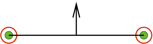
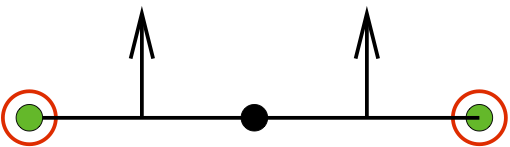
$p=2,\,r=3$	$p=2,\,r=4$
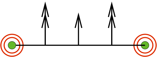
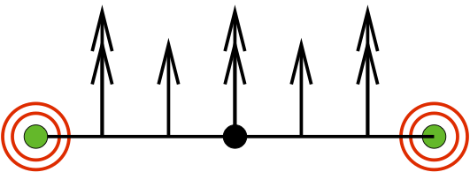
$p=3,\,r=5$	$p=3,\,r=6$

Figure 1: [Taken from [9]]. Edge degrees of freedom of the virtual element space $V^{p}_{h,r}(\textsf{P})$ for the polyharmonic problem with $p=1$ (top panels, Laplace operator), $p=2$ (middle panels, bi-harmonic operator), $p=3$ (bottom panels, triharmonic operator). Here, $p$ is the order of the partial differential operator; $r=1,2,\ldots,6$ are the integer parameters that specify the degree of the polynomial subspace $\mathbbm{P}_{r}(\textsf{P})$ of the VEM space $V_{h,r}^{3}(\textsf{P})$. The (green) dots at the vertices represent the vertex values and each (red) vertex circle represents an order of derivation. The (black) dot on the edge represents the moment of ${v_{h}}_{|{e}}$; the arrows represent the moments of ${\partial_{n}v_{h}}_{|{e}}$; the double arrows represent the moments of ${\partial_{nn}v_{h}}_{|{e}}$. The corresponding internal degrees of freedom (D4) are absent in the case $r=2p-1$, while reduce to a single one in the case $r=2p$.

Finally, we note that in general the internal degrees of freedom (D4) make it possible to define the $L^{2}$-orthogonal polynomial projection of $v_{h}$ onto the space of polynomial of degree $r-2p$.

The dimension of $V^{p}_{h,r}(\textsf{P})$ is

$$d(V^{p}_{h,r}(\textsf{P})) =\frac{p(p+1)}{2}N^{\mathcal{P}}+N^{\mathcal{P}}\sum_{j=0}^{p-1}(r-2p+j+1)+\frac{(r-2p+1)(r-2p+2)}{2},$$

where $N^{\mathcal{P}}$ is the number of vertices, which equals the number of edges, of P.

In [9], it is proved that the above choice of degrees of freedom is unisolvent in $V^{p}_{h,r}(\textsf{P})$.

Building upon the local spaces $V^{p}_{h,r}(\textsf{P})$ for all $\textsf{P}\in\Omega_{h}$, the global conforming virtual element space $V^{p}_{h,r}$ is defined on $\Omega$ as

$$V^{p}_{h,r}=\Big{\{}v_{h}\in H^{p}_{{0}}(\Omega)\,:\,{v_{h}}_{|{\textsf{P}}}\in V^{p}_{h,r}(\textsf{P})\,\,\forall\textsf{P}\in\Omega_{h}\Big{\}}.$$ (12)

We remark that the associated global space is made of $H^{p}(\Omega)$ functions. Indeed, the restriction of a virtual element function $v_{h}$ to each element P belongs to $H^{p}(\textsf{P})$ and glues with $C^{p-1}$-regularity across the internal mesh faces. The set of global degrees of freedom inherited by the local degrees of freedom are:

• $h_{\mathsf{v}}^{|\nu|}D^{\nu}v_{h}(\mathsf{v})$, $\left|\nu\right|\leq p-1$ for every interior vertex $\mathsf{v}$ of $\Omega_{h}$;

• $\displaystyle h_{e}^{-1}\int_{e}qv_{h}\,ds$ for any $q\in\mathbbm{P}_{r-2p}(e)$ and every interior edge $e\in\mathcal{E}_{h}$;

• $\displaystyle h_{e}^{-1+j}\int_{e}q\partial^{j}_{n}v_{h}\,ds$ for any $q\in\mathbbm{P}_{r-2p+j}(e)$ $j=1,\ldots,p-1$ and every interior edge $e\in\mathcal{E}_{h}$;

• $\displaystyle h_{\textsf{P}}^{-2}\int_{\textsf{P}}qv_{h}\,d\mathbf{x}$ for any $q\in\mathbbm{P}_{r-2p}(\textsf{P})$ and every $\textsf{P}\in\Omega_{h}$.

2.2.2 Modified lowest order virtual element spaces

In this section, we briefly discuss the possibility of introducing modified lowest order virtual element spaces with a reduced number of degrees of freedom with respect to the corresponding lowest order ones that were introduced previously. The price we pay is a reduced order of accuracy since the polynomial functions included in such modified spaces has a lower degree.

For the sake of presentation we start from the case $p=3$, while we refer the reader to [36] for the case of $p=2$ and Section 3.2.1 where the reduced virtual space is employed in the context of the approximation of the Cahn-Hilliard problem. Consider the modified local virtual element space:

$$\tilde{V}_{h,5}^{3}(\textsf{P})=\Big{\{}v_{h}\in H^{3}(\textsf{P})\,:\,\Delta^{3}v_{h}=0,v_{h}\in\mathbbm{P}_{5}(e),\,\partial_{n}v_{h}\in\mathbbm{P}_{3}(e),\,\\[5.0pt] \partial_{nn}v_{h}\in\mathbbm{P}_{2}(e)~{}\forall e\in\partial\textsf{P}\Big{\}}$$

with associated degrees of freedom:

(D1’) $h_{\mathsf{v}}^{|\nu|}D^{\nu}v_{h}(\mathsf{v})$, $\left|\nu\right|\leq 2$ for any vertex $\mathsf{v}$ of $\partial\textsf{P}$;

(D2’) $\displaystyle h_{e}\int_{e}\partial_{nn}v_{h}\,ds$ for any edge $e$ of $\partial\textsf{P}$.

In Ref. [9], we proved that the degrees of freedom (D1’) and (D2’) are unisolvent in $\tilde{V}_{h,5}^{3}(\textsf{P})$ and this space contains the linear subspace of polynomials of degree up to $4$. Moreover, the associated global space obtained by gluing together all the elemental spaces $\tilde{V}_{h,5}^{3}(\textsf{P})$ reads as:

$$\tilde{V}_{h,5}^{3}=\Big{\{}v_{h}\in H^{3}_{0}(\Omega)\,:\,v_{h}|_{\textsf{P}}\in\tilde{V}_{h,5}^{3}(\textsf{P})\,\,\forall\textsf{P}\in\Omega_{h}\Big{\}},$$ (13)

is made of $H^{3}(\Omega)$ functions.

Analogously, in the general case we can build the modified lowest order spaces containing the space of polynomials of degree up to $2p-2$:

$$\tilde{V}^{p}_{h,2p-1}(\textsf{P})=\Big{\{}v_{h}\in H^{p}(\textsf{P}):\,\Delta^{p}v_{h}=0,v_{h}\in\mathbbm{P}_{2p-1}(e),\,\partial^{i}_{n}v_{h}\in\mathbbm{P}_{2p-2-i}(e),\\[5.0pt] \,i=1,\ldots,p-1~{}\forall e\in\partial\textsf{P}\Big{\}},$$

with associated degrees of freedom:

(D1’) $h_{\mathsf{v}}^{|\nu|}D^{\nu}v_{h}(\mathsf{v})$, $\left|\nu\right|\leq p-1$ for any vertex $\mathsf{v}$ of $\partial\textsf{P}$;

(D2’) $\displaystyle h_{e}^{-1+j}\int_{e}q\partial_{n}^{i}v_{h}\,ds$ for any $q\in\mathbbm{P}_{j-2}(e)$ and edge $e$ of $\partial\textsf{P}$, $j=1,\ldots,p-1$.

2.2.3 Discrete bilinear form

To define the elliptic projection $\Pi^{\nabla,\textsf{P}}_{r}:V^{p}_{h,r}(\textsf{P})\to\mathbbm{P}_{r}(\textsf{P})$, we first need to introduce the vertex average projector $\widehat{\Pi}^{\textsf{P}}:V^{p}_{h,r}(\textsf{P})\to\mathbbm{P}_{0}(\textsf{P})$, which projects any smooth enough function defined on P onto the space of constant polynomials. To this end, consider the continuous function $\psi$ defined on P. The vertex average projection of $\psi$ onto the constant polynomial space is given by:

$$\widehat{\Pi}^{\textsf{P}}\psi=\frac{1}{N^{\mathcal{P}}}\sum_{\mathsf{v}\in\partial\textsf{P}}\psi(\mathsf{v}).$$ (14)

Finally, we define the elliptic projection $\Pi^{\nabla,\textsf{P}}_{r}:V^{p}_{h,r}(\textsf{P})\to\mathbbm{P}_{r}(\textsf{P})$ as the solution of the following finite dimensional variational problem

$$a_{\textsf{P}}(\Pi^{\nabla,\textsf{P}}_{r}v_{h},q) =a_{\textsf{P}}(v_{h},q)\phantom{\widehat{\Pi}^{\textsf{P}}D^{\nu}v_{h}}\forall q\in\mathbbm{P}_{r}(\textsf{P}),$$ (15)

$$\widehat{\Pi}^{\textsf{P}}D^{\nu}\Pi^{\nabla,\textsf{P}}_{r}v_{h} =\widehat{\Pi}^{\textsf{P}}D^{\nu}v_{h}\phantom{a_{\textsf{P}}(v_{h},q)}\left|\nu\right|\leq{p-1}.$$ (16)

According to Reference [9], such operator has two important properties:

• it is a polynomial-preserving operator in the sense that $\Pi^{\nabla,\textsf{P}}_{r}q=q$ for every $q\in\mathbbm{P}_{r}(\textsf{P})$;

• $\Pi^{\nabla,\textsf{P}}_{r}v_{h}$ is computable using only the degrees of freedom of $v_{h}$.

We write the symmetric bilinear form $a_{h}:V^{p}_{h,r}\times V^{p}_{h,r}\to\mathbbm{R}$ as the sum of local terms

$$a_{h}(u_{h},v_{h})=\sum_{\textsf{P}\in\Omega_{h}}a_{h,\textsf{P}}(u_{h},v_{h}),$$ (17)

where each local term $a_{h,\textsf{P}}:V^{p}_{h,r}(\textsf{P})\times V^{p}_{h,r}(\textsf{P})\to\mathbbm{R}$ is a symmetric bilinear form. We set

$$a_{h,\textsf{P}}(u_{h},v_{h})=a_{\textsf{P}}(\Pi^{\nabla,\textsf{P}}_{r}u_{h},\Pi^{\nabla,\textsf{P}}_{r}v_{h})+S^{\textsf{P}}(u_{h}-\Pi^{\nabla,\textsf{P}}_{r}u_{h},v_{h}-\Pi^{\nabla,\textsf{P}}_{r}v_{h}),$$ (18)

where $S^{\textsf{P}}:V^{p}_{h,r}(\textsf{P})\times V^{p}_{h,r}(\textsf{P})\to\mathbbm{R}$ is a symmetric positive definite bilinear form such that

$$\sigma_{*}a_{\textsf{P}}(v_{h},v_{h})\leq S^{\textsf{P}}(v_{h},v_{h})\leq\sigma^{*}a_{\textsf{P}}(v_{h},v_{h})\qquad\forall v_{h}\in V^{p}_{h,r}(\textsf{P})\textrm{~{}with~{}}\Pi^{\nabla,\textsf{P}}_{r}v_{h}=0,$$ (19)

for two some positive constants $\sigma_{*}$, $\sigma^{*}$ independent of $h$ and P. The bilinear form $a_{h,\textsf{P}}(\cdot,\cdot)$ has the two fundamental properties of $r$-consistency and stability [9]:

$(i)$

$r$-Consistency: for every polynomial $q\in\mathbbm{P}_{r}(\textsf{P})$ and function $V^{p}_{h,r}(\textsf{P})$ we have:

$$a_{h,\textsf{P}}(v_{h},q)=a_{\textsf{P}}(v_{h},q);$$ (20)

$(ii)$

Stability: there exist two positive constants $\alpha_{*}$, $\alpha^{*}$ independent of $h$ and P such that for every $v_{h}\in V^{p}_{h,r}(\textsf{P})$ it holds:

$$\alpha_{*}a_{\textsf{P}}(v_{h},v_{h})\leq a_{h,\textsf{P}}(v_{h},v_{h})\leq\alpha^{*}a_{\textsf{P}}(v_{h},v_{h}).$$ (21)

2.2.4 Discrete load term

We denote by $f_{h}$ the piecewise polynomial approximation of $f$ on $\Omega_{h}$ given by

$${f_{h}}_{|{\textsf{P}}}=\Pi^{0,\textsf{P}}_{r-p}f,$$ (22)

for $r\geq 2p-1$ and $\textsf{P}\in\Omega_{h}$. Then, we set

$$\big{<}f_{h},v_{h}\big{>}=\sum_{\textsf{P}\in\Omega_{h}}\int_{\textsf{P}}f_{h}v_{h}\,\,d\mathbf{x}$$ (23)

which implies, using the $L^{2}$-orthogonal projection, that

$$\big{<}f_{h},v_{h}\big{>}=\sum_{\textsf{P}\in\Omega_{h}}\int_{\textsf{P}}\Pi^{0,\textsf{P}}_{r-p}\,f\Pi^{0,\textsf{P}}_{r-p}v_{h}\,\,d\mathbf{x}=\sum_{\textsf{P}\in\Omega_{h}}\int_{\textsf{P}}f\,\Pi^{0,\textsf{P}}_{r-p}v_{h}\,\,d\mathbf{x}.$$ (24)

The right-hand side of (24) is computable by a combined use of the degrees of freedom (D1)-(D4) and the enhanced approach of Reference [2].

2.2.5 VEM spaces with arbitrary degree of continuity

In this section we briefly sketch the construction of global virtual element spaces with arbitrary high order of continuity. More precisely, we consider the local virtual element space defined as before, for $r\geq 2p-1$:

$$V^{p}_{h,r}(\textsf{P})=\Big{\{}v_{h}\in H^{p}(\textsf{P}):\,\Delta^{p}v_{h}\in\mathbbm{P}_{r-2p}(\textsf{P}),\,v_{h}\in\mathbbm{P}_{r}(e),\,\partial^{j}_{n}v_{h}\in\mathbbm{P}_{r-j}(e),\,\\[5.0pt] j=1,\ldots,p-1~{}\forall e\in\partial\textsf{P}\big{\}}.$$

Differently from the previous section, we make the degrees of freedom depend on a given parameter $t$ with $0\leq t\leq p-1$. For a given value of $t$ we choose the degrees of freedom as follows

(D1) $h_{\mathsf{v}}^{|\nu|}D^{\nu}v_{h}(\mathsf{v})$, $\left|\nu\right|\leq p-1$ for any vertex $\mathsf{v}$ of P;

(D2) $\displaystyle h_{e}^{-1}\int_{e}v_{h}q\,ds$ for any $q\in\mathbbm{P}_{r-2p}(e)$,  for any edge $e$ of $\partial\textsf{P}$;

(D3) $\displaystyle h_{e}^{-1+j}\int_{e}\partial^{j}_{n}v_{h}q\,ds$ for any $q\in\mathbbm{P}_{r-2p+j}(e)$ and edge $e\in\partial\textsf{P}$, $j=1,\ldots,p-1$;

(D4’) $\displaystyle h_{\textsf{P}}^{-2}\int_{\textsf{P}}qv_{h}\,\,d\mathbf{x}$ for any $q\in\mathbbm{P}_{r-2(p-t)}(\textsf{P})$;

where as usual we assume $\mathbbm{P}_{-n}(\cdot)=\{0\}$ for $n=1,2,3,\ldots$.

This set of degrees is still unisolvent, cf. [9]. Moreover, for $r\geq 2p-1$ it holds that $\mathbbm{P}_{r}(\textsf{P})\subset V^{p}_{h,r}(\textsf{P})$. Finally, it is worth noting that the choice (D4’), if compared with (D4), still guarantees that the associated global space is made of $C{p-1}$ functions.

However, in this latter case we can use the degrees of freedom (D1)-(D4’) to solve a differential problem involving the $\Delta^{p-t}$ operator and $C^{p-1}(\Omega)$ basis functions. For the sake of exposition, let us consider the following two examples, in the context of the Laplacian and the Bilaplacian problem.

1. Choosing $p$ and $t$ such that $p-t=1$ we obtain a $C^{p-1}$-conforming virtual element method for the solution of the Laplacian problem. For example, for $p=3$, $t=2$ and $r=5$, the local space $V^{3}_{h,5}(\textsf{P})$ endowed with the corresponding degrees of freedom (D1)-(D4’) can be employed to build a global space made of $C^{2}$ functions. It is also worth mentioning that the new choice (D4’), differently from the original choice (D4), is essential for the computability of the elliptic projection, see (15)-(16), with respect to the bilinear form $a_{\textsf{P}}(\cdot,\cdot)=\int_{\textsf{P}}\nabla(\cdot)\nabla(\cdot)\,\,d\mathbf{x}$.

2. Choosing $p$ and $t$ such that $p-t=2$ we have a $C^{p-1}$-conforming virtual element method for the solution of the Bilaplacian problem. For example, for $p=3$, $t=1$ and $r=5$, similarly to the previous case, the space $V^{3}_{h,5}(\textsf{P})$ together with (D1)-(D4’) provides a global space of $C^{2}$ functions that can be employed for the solution of the biharmonic problem.

It is worth remembering that $C^{1}$-regular virtual element basis function has been employed, e.g., in [25] to study residual based a posteriori error estimators for the virtual element approximation of second order elliptic problems. Moreover, the solution of coupled elliptic problems of different order can take advantage from this flexibility of the degree of continuity of the basis functions. Indeed, for the sake of clarity consider the conforming virtual element approximation of the following simplified situation:

$$-\Delta u_{1} =f_{1}\phantom{f_{2}u_{1}\partial_{n}u_{2}0}\text{in~{}}\Omega_{1},$$

$$\Delta^{2}u_{2} =f_{2}\phantom{f_{1}u_{1}\partial_{n}u_{2}0}\text{in~{}}\Omega_{2},$$

$$u_{1} =u_{2}\phantom{f_{1}f_{2}\partial_{n}u_{2}0}\text{on~{}}\Gamma=\Omega_{1}\cap\Omega_{2},$$

$$\partial_{n}u_{1} =\partial_{n}u_{2}\phantom{f_{1}f_{1}u_{1}0}\text{on~{}}\Gamma,$$

$$u_{1} =0\phantom{f_{1}f_{2}u_{2}\partial_{n}u_{2}}\text{on~{}}\partial\Omega_{1}\setminus\Gamma,$$

$$u_{2} =0\phantom{f_{1}f_{2}u_{2}\partial_{n}u_{2}}\text{on~{}}\partial\Omega_{2}\setminus\Gamma,$$

$$\partial_{n}u_{2} =0\phantom{f_{1}f_{2}u_{2}\partial_{n}u_{2}}\text{on~{}}\partial\Omega_{2}\setminus\Gamma.$$

Handling the coupling conditions on $\Gamma$ asks for the use of $C^{1}$-regular virtual basis functions not only in $\Omega_{2}$ where the bilaplacian problem is defined, but also in $\Omega_{1}$, where the second order elliptic problem is defined. Indeed, a simple use of $C^{0}$-basis functions in $\Omega_{1}$, which would be natural given the second order of the problem, would not allow the imposition (or at least a simple imposition) of the gluing condition on the normal derivatives.

2.2.6 Convergence results

The following convergence result in the energy norm holds (see [9] for the proof).

Theorem 2.1

Let $f\in H^{r-p+1}(\Omega)$ be the forcing term at the right-hand side, $u$ the solution of the variational problem (6) and $u_{h}\in V^{p}_{h,r}$ the solution of the virtual element method (11). Then, it holds that

$$\left|\!\left|u-u_{h}\right|\!\right|_{\mathsf{v}}\leq Ch^{r-(p-1)}\big{(}|u|_{r+1}+|f|_{r-p+1}\big{)}.$$ (25)

Moreover, the following convergence results in lower order norms can established [9].

Theorem 2.2 (Even $p$, even norms)

Let $f\in H^{r-p+1}(\Omega)$, $u$ the solution of the variational problem (6) with $p=2\ell$ and $v_{h}\in V^{p}_{h,r}$ the solution of the virtual element method (11). Then, there exists a positive constant $C$ independent of $h$ such that

$$|u-u_{h}|_{2i}\leq Ch^{r+1-2i}\Big{(}|u|_{r+1}+|f|_{r-(p-1)}\Big{)},$$ (26)

for every integer $i=0,\ldots,\ell-1$.

Theorem 2.3 (Even $p$, odd norms)

Let $f\in H^{r-p+1}(\Omega)$, and $u$ the solution of the variational problem (6) with $p=2\ell$ and $u_{h}\in V^{p}_{h,r}$ the solution of the virtual element method (11). Then, there exists a positive constant $C$ independent of $h$ such that

$$|u-u_{h}|_{2i+1}\leq Ch^{(r+1)-(2i+1)}\Big{(}|u|_{r+1}+|f|_{r-(p-1)}\Big{)},$$ (27)

for every integer $i=0,\ldots,\ell-1$.

Theorem 2.4 (Odd $p$, even norms)

Let $u$ be the solution of the variational problem (6) and $u_{h}\in V^{p}_{h,r}$ the solution of the virtual element method (11). Then, there exists a positive constant $C$ independent of $h$ such that

$$|u-u_{h}|_{2i}\leq Ch^{(r+1)-2i}\Big{(}|u|_{r+1}+|f|_{r-(p-1)}\Big{)},$$ (28)

for every integer $i=0,\ldots,\ell-1$.

Theorem 2.5 (Odd $p$, odd norms)

Let $u$ be the solution of the variational problem (6) and $u_{h}\in V^{p}_{h,r}$ the solution of the virtual element method (11). Then, there exists a positive constant $C$ independent of $h$ such that

$$|u-u_{h}|_{2i+1}\leq Ch^{(r+1)-(2i+1)}\Big{(}|u|_{r+1}+|f|_{r-(p-1)}\Big{)},$$ (29)

for every integer $i=0,\ldots,\ell-1$.

3 The virtual element method for the Cahn-Hilliard problem

3.1 The continuous problem

Let $\Omega\subset\mathbbm{R}^{2}$ be an open, bounded domain with polygonal boundary $\Gamma$, $\psi:\mathbbm{R}\to\mathbbm{R}$ with $\psi(x)=(1-x^{2})^{2}/4$ and $\phi(x)=\psi^{\prime}(x)$. We consider the Cahn-Hilliard problem: Find $u(x,t):\Omega\times[0,T]\rightarrow\mathbbm{R}$ such that:

$$\dot{u}-\Delta\big{(}\phi(u)-\gamma^{2}\Delta u\big{)}=0\phantom{u_{0}(\cdot)} \quad\textrm{in~{}}\Omega\times[0,T],$$ (30a)

$$u(\cdot,0)=u_{0}(\cdot)\phantom{0} \quad\textrm{in~{}}\Omega,$$ (30b)

$$\partial_{n}u=\partial_{n}\big{(}\phi(u)-\gamma^{2}\Delta u\big{)}=0\phantom{u_{0}(\cdot)} \quad\textrm{on~{}}\partial\Omega\times[0,T],$$ (30c)

where $\partial_{n}$ denotes the (outward) normal derivative and $\gamma\in\mathbbm{R}^{+}$, $0<\gamma\ll 1$, represents the interface parameter. On the domain boundary we impose a no flux-type condition on $u$ and the chemical potential $\phi(u)-\gamma^{2}\Delta u$.

To define the variational formulation of problem (30a)-(30c) we introduce the three bilinear forms:

$$a^{\Delta}(v,w) =\int_{\Omega}(\nabla^{2}v):(\nabla^{2}w)\,d\mathbf{x} \quad\forall v,w\in H^{2}(\Omega),$$

$$a^{\nabla}(v,w) =\int_{\Omega}\nabla v\cdot\nabla w\,d\mathbf{x} \quad\forall v,w\in H^{1}(\Omega),$$

$$a^{0}(v,w) =\int_{\Omega}v\,w\,d\mathbf{x} \quad\forall v,w\in L^{2}(\Omega),$$

($\nabla^{2}$ being the Hessian operator) and the semi-linear form

$$r(z;v,w)=\int_{\Omega}\phi^{\prime}(z)\nabla v\cdot\nabla w\,d\mathbf{x}\quad\forall z,v,w\in H^{2}(\Omega).$$

Finally, introducing the functional space

$$V=\big{\{}v\in H^{1}(\Omega)\,:\,\partial_{n}{v}=0\textrm{~{}on~{}}\Gamma\big{\}},$$ (31)

which is a subspace of $H^{1}(\Omega)$.

The weak formulation of problem (30a)-(30c) reads as: Find $u(\cdot,t)\in V$ such that

$$a^{0}(\dot{u},v)+\gamma^{2}a^{\Delta}(u,v)+r(u;u,v)=0\quad\forall v\in V,$$ (32a)

$$u(\cdot,0)=u_{0}.$$ (32b)

3.2 The conforming Virtual Element approximation

In this section, we introduce the main building blocks for the conforming virtual discretization of the Cahn-Hilliard equation, report a convergence result and collect some numerical results assessing the theoretical properties of the proposed scheme.

3.2.1 A $C^{1}$ Virtual Element space

We briefly recall the construction of the virtual element space ${W}_{h}\subset H^{2}(\Omega)$ that we use to discretize (32a)-(32b); see [5] for more details.

Given an element $\textsf{P}\in\Omega_{h}$, the augmented local space $\widetilde{V}_{h|\textsf{P}}$ is defined by

$$\widetilde{V}_{h|\textsf{P}}=\Big{\{}v\in H^{2}(\textsf{P})\,:\, \Delta^{2}v\in\mathbbm{P}_{2}(\textsf{P}),{v}_{|{\partial\textsf{P}}}\in C^{0}(\partial\textsf{P}),{v}_{|{e}}\in\mathbbm{P}_{3}(e)\quad\forall e\in\partial\textsf{P},$$

$${\nabla v}_{|{\partial\textsf{P}}}\in\big{[}C^{0}(\partial\textsf{P})\big{]}^{2},\partial_{n}{v}_{|{e}}\in\mathbbm{P}_{1}(e)\quad\forall e\in\partial\textsf{P}\Big{\}},$$ (33)

with $\partial_{n}$ denoting the (outward) normal derivative.

Remark 3.1

The space $\widetilde{V}_{h|\textsf{P}}$ corresponds to the space $\tilde{V}^{p}_{h,2p-1}(\textsf{P})$ with $p=2$ introduced in Section 2.2.2.

We consider the two sets of linear operators from $\widetilde{V}_{h|\textsf{P}}$ into $\mathbb{R}$ denoted by (D1) and (D2) and defined as follows:

(D1) contains linear operators evaluating $v_{h}$ at the $n=n(\textsf{P})$ vertices of P;

(D2) contains linear operators evaluating $\nabla v_{h}$ at the $n=n(\textsf{P})$ vertices of P.

The output values of the two sets of operators (D1) and (D2) are sufficient to uniquely determine $v_{h}$ and $\nabla v_{h}$ on the boundary of P (cf. Section 2.2.2).

We use of the following local bilinear forms for all $\textsf{P}\in\Omega_{h}$

$$a_{\textsf{P}}^{\Delta}(v,w) =\int_{\textsf{P}}(\nabla^{2}v):(\nabla^{2}w)\,d\mathbf{x}\phantom{\int_{\textsf{P}}v\,w\,d\mathbf{x}}\forall v,w\in H^{2}(\textsf{P}),$$ (34)

$$a_{\textsf{P}}^{\nabla}(v,w) =\int_{\textsf{P}}\nabla v\cdot\nabla w\,d\mathbf{x}\quad\forall v,w\in H^{1}(\textsf{P}),$$ (35)

$$a_{\textsf{P}}^{0}(v,w) =\int_{\textsf{P}}v\,w\,d\mathbf{x}\phantom{\int_{\textsf{P}}(\nabla^{2}v):(\nabla^{2}w)\,d\mathbf{x}}\forall v,w\in L^{2}(\textsf{P}).$$ (36)

Now, we introduce the elliptic projection operator $\Pi^{\Delta,\textsf{P}}_{2}\colon\widetilde{V}_{h|\textsf{P}}\rightarrow\mathbbm{P}_{2}(\textsf{P})$ defined by

$$a_{\textsf{P}}^{\Delta}(\Pi^{\Delta,\textsf{P}}_{2}v_{h},q) =a_{\textsf{P}}^{\Delta}(v_{h},q)\phantom{(\!(v_{h},q)\!)_{\textsf{P}}}\forall q\in\mathbbm{P}_{2}(\textsf{P}),$$ (37)

$$(\!(\Pi^{\Delta,\textsf{P}}_{2}v_{h},q)\!)_{\textsf{P}} =(\!(v_{h},q)\!)_{\textsf{P}}\phantom{a_{\textsf{P}}^{\Delta}(v_{h},q)}\forall q\in\mathbbm{P}_{1}(\textsf{P}),$$ (38)

for all $v_{h}\in\widetilde{V}_{h|\textsf{P}}$ where $(\!(\cdot,\cdot)\!)_{\textsf{P}}$ is the Euclidean scalar product acting on the vectors that collect the vertex function values, i.e.

$$(\!(v_{h},w_{h})\!)_{\textsf{P}}=\sum_{\mathsf{v}\in\mathcal{V}_{\textsf{P}}}\!\!v_{h}(\mathsf{v})\>w_{h}(\mathsf{v})\quad\forall v_{h},w_{h}\in C^{0}(\textsf{P}).$$

As shown in [5], the operator $\Pi^{\Delta,\textsf{P}}_{2}\colon\widetilde{V}_{h|\textsf{P}}\rightarrow\mathbbm{P}_{2}(\textsf{P})$ is well defined and uniquely determined on the basis of the information carried by the linear operators in (D1) and (D2).

Hinging upon the augmented space $\widetilde{V}_{h|\textsf{P}}$ and employing the projector $\Pi^{\Delta,\textsf{P}}_{2}$ we define our virtual local space

$$W_{h|\textsf{P}}=\big{\{}v\in\widetilde{V}_{h|\textsf{P}}\,:\,a_{\textsf{P}}^{0}(\Pi^{\Delta,\textsf{P}}_{2}(v),q)=a_{\textsf{P}}^{0}(v,q)\quad\forall q\in\mathbbm{P}_{2}(\textsf{P})\big{\}}.$$ (39)

Since $W_{h|\textsf{P}}\subset\widetilde{V}_{h|\textsf{P}}$, operator $\Pi^{\Delta,\textsf{P}}_{2}$ is well defined on $W_{h|\textsf{P}}$ and computable by using the values provided by (D1) and (D2). Moreover, the set of operators (D1) and (D2) constitutes a set of degrees of freedom for the space $W_{h|\textsf{P}}$. Finally, there holds $\mathbbm{P}_{2}(\textsf{P})\subseteq W_{h|\textsf{P}}$.

We now introduce two further projectors on the local space $W_{h|\textsf{P}}$, namely $\Pi^{0,\textsf{P}}_{2}$ and $\Pi^{\nabla,\textsf{P}}_{2}$, that will be employed together with the above projector $\Pi^{\Delta,\textsf{P}}_{2}$ to build the discrete counterparts of the bilinear forms in (34). Operator $\Pi^{0,\textsf{P}}_{2}:W_{h|\textsf{P}}\rightarrow\mathbbm{P}_{2}(\textsf{P})$ is the standard $L^{2}$ projector on the space of quadratic polynomials in P. This is computable by means of the values of the degrees of freedom (D1) and (D2) (cf. [5]). To define $\Pi^{\nabla,\textsf{P}}_{2}:W_{h|\textsf{P}}\rightarrow\mathbbm{P}_{2}(\textsf{P})$ we need the additional bilinear form $a^{\nabla}(\cdot,\cdot):W_{h|\textsf{P}}\times W_{h|\textsf{P}}\to\mathbbm{R}$ that is given by

$$a^{\nabla}(v,w)=\int_{\Omega}\nabla v\cdot\nabla w\,d\mathbf{x}\quad\forall v,w\in H^{1}(\Omega).$$

Operator $\Pi^{\nabla,\textsf{P}}_{2}$ is the elliptic projection defined with respect to $a^{\nabla}(\cdot,\cdot)$:

$$a_{\textsf{P}}^{\nabla}(\Pi^{\nabla,\textsf{P}}_{2}v_{h},q) =a_{\textsf{P}}^{\nabla}(v_{h},q)\quad\forall q\in\mathbbm{P}_{2}(\textsf{P}),$$ (40a)

$$\int_{\textsf{P}}\Pi^{\nabla,\textsf{P}}_{2}v_{h}d\mathbf{x} =\int_{\textsf{P}}v_{h}\,d\mathbf{x}.$$ (40b)

Such operator is well defined and uniquely determined by the values of (D1) and (D2) [5].

We are now ready to introduce the global virtual element space, which defined as follows

$${W}_{h}=\big{\{}v\in V\,:\,{v}_{|{\textsf{P}}}\in W_{h|\textsf{P}}\quad\forall\textsf{P}\in\Omega_{h}\big{\}}.$$

The virtual element functions in ${W}_{h}$ and their gradients are continuous fields on $\Omega$, so this functional space is a conforming subspace of $H^{2}(\Omega)$. The global degrees of freedom of ${W}_{h}$ are obtained by collecting the elemental degrees of freedom, so the dimension of ${W}_{h}$ is three times the number of the mesh vertices, and every virtual element function $v_{h}$ defined on $\Omega$ is uniquely determined by

• $(i)$ its values at the mesh vertices;

• $(ii)$ its gradient values at the mesh vertices.

Finally, we recommended to scale the degrees of freedom (D2) by some local characteristic mesh size $h_{\mathsf{v}}$ in order to obtain a better condition number of the final system.

3.2.2 Virtual element bilinear forms

We start by introducing the discrete versions of the elemental bilinear form forms in (34). Let $\textsf{P}\in\Omega_{h}$ be a generic mesh element and $s_{\textsf{P}}(\cdot,\cdot):W_{h|\textsf{P}}\times W_{h|\textsf{P}}\to\mathbbm{R}$ the positive definite bilinear form given by:

$$s_{\textsf{P}}(v_{h},w_{h})=\sum_{\mathsf{v}\in\mathcal{V}_{\textsf{P}}}\!\!\Big{(}v_{h}(\mathsf{v})\>w_{h}(\nu)+h_{\mathsf{v}}^{2}\>\nabla v_{h}(\mathsf{v})\cdot\nabla w_{h}(\mathsf{v})\Big{)}\quad\forall v_{h},w_{h}\in W_{h|\textsf{P}},$$

where $h_{\mathsf{v}}$ is a characteristic mesh size length associated with node $\mathsf{v}$, e.g., the maximum diameter among the elements having $\mathsf{v}$ as a vertex.

Recalling (34), we consider the virtual element bilinear forms:

$$a_{h,\textsf{P}}^{\Delta}(v_{h},w_{h}) =a_{\textsf{P}}^{\Delta}(\Pi^{\Delta,\textsf{P}}_{2}v_{h},\Pi^{\Delta,\textsf{P}}_{2}w_{h})+h_{\textsf{P}}^{-2}s_{\textsf{P}}\big{(}v_{h}-\Pi^{\Delta,\textsf{P}}_{2}v_{h},w_{h}-\Pi^{\Delta,\textsf{P}}_{2}w_{h}\big{)},$$ (41)

$$a_{h,\textsf{P}}^{\nabla}(v_{h},w_{h}) =a_{\textsf{P}}^{\nabla}(\Pi^{\nabla,\textsf{P}}_{2}v_{h},\Pi^{\nabla,\textsf{P}}_{2}w_{h})+s_{\textsf{P}}\big{(}v_{h}-\Pi^{\nabla,\textsf{P}}_{2}v_{h},w_{h}-\Pi^{\nabla,\textsf{P}}_{2}w_{h}),$$ (42)

$$a_{h,\textsf{P}}^{0}(v_{h},w_{h}) =a_{\textsf{P}}^{0}(\Pi^{0,\textsf{P}}_{2}v_{h},\Pi^{0,\textsf{P}}_{2}w_{h})+h_{\textsf{P}}^{2}s_{\textsf{P}}\big{(}v_{h}-\Pi^{0,\textsf{P}}_{2}v_{h},w_{h}-\Pi^{0,\textsf{P}}_{2}w_{h}\big{)}$$ (43)

for all $v_{h}$, $w_{h}\in W_{h|\textsf{P}}$. Under the mesh regularity conditions of Section 1.2, we can prove the consistency and stability of the discrete bilinear forms. Let the symbol $\dagger$ stands for “$\Delta$”, “$\nabla$” or “$0$”. We have:

• (A) (polynomial consistency) $a_{h,\textsf{P}}^{\dagger}(p,v_{h})=a_{\textsf{P}}^{\dagger}(p,v_{h})\quad\forall p\in\mathbbm{P}_{2}(\textsf{P}),\,v_{h}\in W_{h|\textsf{P}}$;

• (B) (stability) there exist two positive constants $c_{*}$ and $c^{*}$ independent of $h$ and the element $\textsf{P}\in\Omega_{h}$ such that

  $$c_{*}a_{\textsf{P}}^{\dagger}(v_{h},v_{h})\leq a_{h,\textsf{P}}^{\dagger}(v_{h},v_{h})\leq c^{*}a_{\textsf{P}}^{\dagger}(v_{h},v_{h})\quad\forall v_{h}\in W_{h|\textsf{P}}.$$

A consequence of the above properties is that the bilinear form $a_{h,\textsf{P}}^{\dagger}(\cdot,\cdot)$ is continuous with respect to the relevant norm, which is $H^{2}$ for (41), $H^{1}$ for (42), and $L^{2}$ for (43). For every choice of $\dagger$, the corresponding global bilinear form is

$$a_{h}^{\dagger}(v_{h},w_{h})=\sum_{\textsf{P}\in\Omega_{h}}a_{h,\textsf{P}}^{\dagger}(v_{h},w_{h})\quad\forall v_{h},w_{h}\in{W}_{h}.$$

(30a)-(30c)

We now turn our attention to the semilinear form $r(\cdot;\cdot,\cdot)$, which we can also write as the sum of elemental contributions:

$$r(z;v,w)=\sum_{\textsf{P}\in\Omega_{h}}r_{\textsf{P}}(z;v,w)\quad\forall z,vw\in H^{2}(\Omega)$$

where

$$r_{\textsf{P}}(z;v,w)=\int_{\textsf{P}}(3z^{2}-1)\nabla v\cdot\nabla wd\mathbf{x}\quad\forall\textsf{P}\in\Omega_{h}.$$

On each element P, we approximate the term $z(x)^{2}$ by means of its cell average, which we compute using the $L^{2}(\textsf{P})$ bilinear form $a_{h,\textsf{P}}^{0}(\cdot,\cdot)$:

$${z_{h}^{2}}_{|{\textsf{P}}}\approx\left|\textsf{P}\right|^{-1}a_{h,\textsf{P}}^{0}(z_{h},z_{h}),$$

where we recall that $\left|\textsf{P}\right|$ is the area of element P. This approach has the correct approximation properties and preserves the positivity of $z^{2}$.

We therefore propose the following approximation of the local nonlinear forms

$$r_{h,\textsf{P}}(z_{h};v_{h},w_{h})={\widehat{\phi^{\prime}(z_{h})}}_{|{\textsf{P}}}\>a_{h,\textsf{P}}^{\nabla}(v_{h},w_{h})\quad\forall z_{h},v_{h},w_{h}\in W_{h|\textsf{P}},$$

where ${\widehat{\phi^{\prime}(z_{h})}}_{|{\textsf{P}}}=3\left|\textsf{P}\right|^{-1}a_{h,\textsf{P}}^{0}(z_{h},z_{h})-1$. The global form is then assembled as

$$r_{h}(z_{h};v_{h},w_{h})=\sum_{\textsf{P}\in\Omega_{h}}r_{h,\textsf{P}}(z_{h};v_{h},w_{h})\quad\forall z_{h},v_{h}w_{h}\in{W}_{h}.$$

3.2.3 The discrete problem

The virtual element discretization of problem (32a)(32b) follows a Galerkin approach in space combined with a backward Euler time-stepping scheme. Consider the functional space

$${W}_{h}^{0}={W}_{h}\cap V=\big{\{}v\in{W}_{h}\,:\,\partial_{n}v=0\textrm{~{}on~{}}\partial\Omega\big{\}},$$

which includes the boundary conditions. Then, we introduce the the semi-discrete approximation: Find $u_{h}(\cdot,t)$ in ${W}_{h}^{0}$ such that

$$a_{h}^{0}(\dot{u_{h}},v_{h})+\gamma^{2}a_{h}^{\Delta}(u_{h},v_{h})+r_{h}(u_{h};u_{h},v_{h}) =0\quad\forall v_{h}\in{W}_{h}^{0},$$ (44)

$$u_{h}(0,\cdot)=u_{0,h}(\cdot),$$ (45)

where $u_{0,h}$ is a suitable approximation of $u_{0}$ in ${W}_{h}^{0}$ and $a_{h}^{0}(\cdot,\cdot)$, $a_{h}^{\Delta}$ and $r_{h}$ are the virtual element bilinear forms defined in the previous section.

To formulate the fully discrete scheme, we subdivide the time interval $[0,T]$ into $N$ uniform sub-intervals of length $k=T/N$ by means of the time nodes $0=t_{0}<t_{1}<\ldots<t_{N-1}<t_{N}=T$, and denote the virtual element approximation of the solution $u(\cdot,t)$ at $u(\cdot,t^{i})$ in ${W}_{h}^{0}$ by $u_{h,k}^{i}$. The fully discrete problem reads as: Given $u_{hk}^{0}=u_{0,h}\in{W}_{h}^{0}$, find $u_{hk}^{i}\in{W}_{h}^{0}$, $i=1,\ldots,N$ such that

$$k^{-1}a_{h}^{0}(u_{hk}^{i}-u_{hk}^{i-1},v_{h})+\gamma^{2}a_{h}^{\Delta}(u_{hk}^{i},v_{h})+r_{h}(u_{hk}^{i},u_{hk}^{i};v_{h})=0\quad\forall v_{h}\in{W}_{h}^{0}.$$ (46)

The semidiscrete Virtual Element formulation given in (44)-(45) converges to the exact solution of problem (32a)-(32b) according to the result stated in this theorem and proved in [5].

Theorem 3.2

Let $u$ be the solution of problem (32a)-(32b). Let $u_{h}$ be the virtual element approximation provided by (44)-(45) and assume that

$$||u_{h}||_{L^{\infty}(\Omega)}\leq C$$

for all $t\in(0,T]$ and some positive constant $C$ independent of $h$. Then, it holds that

$$\left|\left|u-u_{h}\right|\right|_{L^{2}(\Omega)}\lesssim h^{2}$$

for every $t\in[0,T]$.

3.3 Numerical results

In this test, taken from [5] we study the convergence of our VEM discretization applied to the Cahn-Hilliard problem with a load term $f$ obtained by enforcing as exact solution $u(x,y,t)=t\cos(2\pi x)\cos(2\pi y)$. The parameter $\gamma$ is set to $1/10$ and the time step size $\Delta t$ is $1e-7$. The $H^{2}$, $H^{1}$ and $L^{2}$ errors are computed at $t=0.1$ on four quadrilateral meshes discretizing the unit square. The time discretization is performed by the Backward Euler method. The resulting non-linear system (46) at each time step is solved by the Newton method, using the $l^{2}$ norm of the relative residual as a stopping criterion. The tolerance for convergence is $1e-6$.

Table 1: $H^{2}$, $H^{1}$ and $L^{2}$ errors and convergence rates $\alpha$ computed on four quadrilateral meshes discretizing the unit square [5].

$h$	$|u-u_{h}|_{H^{2}(\Omega)}$	$\alpha$	$|u-u_{h}|_{H^{1}(\Omega)}$	$\alpha$	$\left|\left|u-u_{h}\right|\right|_{L^{2}(\Omega)}$	$\alpha$
1/16	1.35e-1	–	8.57e-2	–	8.65e-2	–
1/32	5.86e-2	1.20	2.20e-2	1.96	2.20e-2	1.97
1/64	2.79e-2	1.07	5.53e-3	1.99	5.52e-3	1.99
1/128	1.38e-2	1.02	1.37e-3	2.01	1.37e-3	2.01

The results reported in Table 1 show that the VEM method converges is convergent with a convergence rate close to $2$ in the $L^{2}$ norm as expected from Theorem 3.2. In the $H^{2}$ and $H^{1}$ seminorms, the method converges with order $1$ and $2$ respectively, as we can expect from the FEM theory and the approximation properties of the virtual element space. Finally, in Figure 2 we report the results of a spinoidal decomposition. For completeness, we recall that spinoidal decomposition is a physical phenomenon consisting of the separation of a mixture of two or more components to bulk regions of each, which occurs when a high-temperature mixture of different components is rapidly cooled. We employ an initial datum $u_{0}$ chosen to be a uniformly distributed random perturbation between $-1$ and $1$. Results are consistent with the literature, cf. [5].

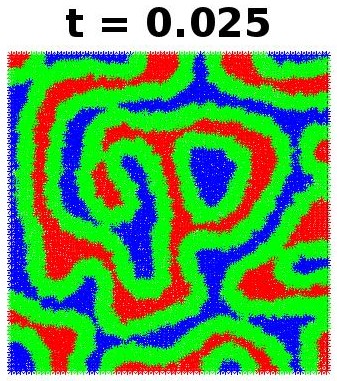
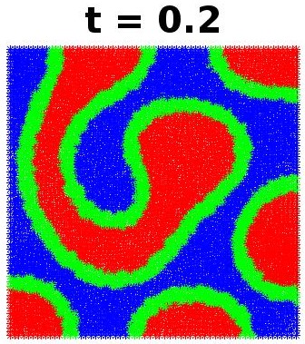
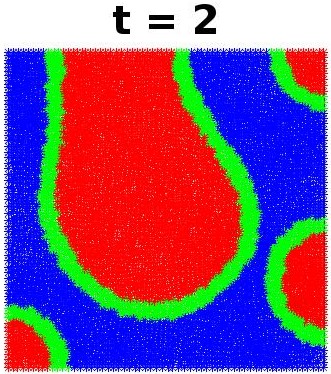
Figure 2: Spinoidal decomposition on the unit square at three temporal frames for a Voronoi polygonal mesh of 4096 elements.

4 The virtual element method for the elastodynamics problem

4.1 The continuous problem

We consider an elastic body occupying the open, bounded polygonal domain $\Omega\subset\mathbbm{R}^{2}$ with Lipschitz boundary $\Gamma$. We assume that boundary $\Gamma$ can be split into the two disjoint subsets $\Gamma_{D}$ and $\Gamma_{N}$, so that $\Gamma=\Gamma_{D}\cup\Gamma_{N}$ and with the one-dimensional Lebesgue measure (length) $\left|\Gamma_{D}\cap\Gamma_{N}\right|=0$. For the well-posedness of the mathematical model, we further require length of $\Gamma_{D}$ is nonzero, i.e., $\left|\Gamma_{D}\right|>0$. Let $T>0$ denote the final time. We consider the external load $\mathbf{f}\in L^{2}\big{(}0,T;[L^{2}(\Omega)]^{2}\big{)}$, the boundary function $\mathbf{g}_{N}\in C^{1}\big{(}0,T;[H^{1/2}_{0,\Gamma_{N}}]^{2}\big{)}$, and the initial functions $\mathbf{u}_{0}\in[H^{1}_{0,\Gamma_{D}}(\Omega)]^{2}$, $\mathbf{u}_{1}\in[L^{2}(\Omega)]^{2}$. For such time-dependent vector fields, we may indicate the dependence on time explicitly, e.g., $\mathbf{f}(t):=\mathbf{f}(\cdot,t)\in[L^{2}(\Omega)]^{2}$, or drop it out to ease the notation when it is obvious from the context.

The equations governing the two-dimensional initial/boundary-value problem of linear elastodynamics for the displacement vector $\mathbf{u}:\Omega\times[0,T]\to\mathbbm{R}^{2}$ are:

$$\rho\ddot{\mathbf{u}}-\nabla\cdot{\bm{\sigma}}(\mathbf{u}) =\mathbf{f}\phantom{\mathbf{0}\mathbf{g}_{N}\mathbf{u}_{0}\mathbf{u}_{1}}\textrm{in}~{}\Omega\times(0,T],$$ (47)

$$\mathbf{u} =\mathbf{0}\phantom{\mathbf{f}\mathbf{g}_{N}\mathbf{u}_{0}\mathbf{u}_{1}}\textrm{on}~{}\Gamma_{D}\times(0,T],$$ (48)

$${\bm{\sigma}}(\mathbf{u})\mathbf{n} =\mathbf{g}_{N}\phantom{\mathbf{f}\mathbf{0}\mathbf{u}_{0}\mathbf{u}_{1}}\textrm{on}~{}\Gamma_{N}\times(0,T],$$ (49)

$$\mathbf{u} =\mathbf{u}_{0}\phantom{\mathbf{f}\mathbf{0}\mathbf{g}_{N}\mathbf{u}_{1}}\textrm{in}~{}\Omega\times\{0\},$$ (50)

$$\dot{\mathbf{u}} =\mathbf{u}_{1}\phantom{\mathbf{f}\mathbf{0}\mathbf{g}_{N}\mathbf{u}_{0}}\textrm{in}~{}\Omega\times\{0\}.$$ (51)

Here, $\rho$ is the mass density, which we suppose to be a strictly positive and uniformly bounded function and ${\bm{\sigma}}(\mathbf{u})$ is the stress tensor. In (48) we assume homogeneous Dirichlet boundary conditions on $\Gamma_{D}$. This assumption is made only to ease the exposition and the analysis, as our numerical method is easily extendable to nonhomogeneous Dirichlet boundary conditions.

We denote the space of the symmetric, $2\times 2$-sized, real-valued tensors by $\mathbb{R}^{2\times 2}_{\textrm{sym}}$ and assume that the stress tensor ${\bm{\sigma}}:\Omega\times[0,T]\to\mathbb{R}^{2\times 2}_{\textrm{sym}}$ is expressed, according to Hooke’s law, by ${\bm{\sigma}}(\mathbf{u})=\mathcal{D}{\bm{\varepsilon}}(\mathbf{u})$, where, ${\bm{\varepsilon}}(\mathbf{u})$ denotes the symmetric gradient of $\mathbf{u}$ , i.e., ${\bm{\varepsilon}}(\mathbf{u})=\big{(}\nabla\mathbf{u}+(\nabla\mathbf{u})^{T}\big{)}/{2}$, and $\mathcal{D}=\mathcal{D}(\mathbf{x})\,\,:\mathbb{R}^{2\times 2}_{\textrm{sym}}\longrightarrow\mathbb{R}^{2\times 2}_{\textrm{sym}}$ is the stiffness tensor

$$\mathcal{D}\bm{\tau}=2\mu\bm{\tau}+\lambda\textrm{tr}(\bm{\tau})\mathsf{I}$$ (52)

for all $\bm{\tau}\in\mathbb{R}^{2\times 2}_{\textrm{sym}}$. In this definition, $\mathsf{I}$ and $\textrm{tr}(\cdot)$ are the identity matrix and the trace operator; $\lambda$ and $\mu$ are the first and second Lamé coefficients, which we assume to be in $L^{\infty}(\Omega)$ and nonnegative. The compressional (P) and shear (S) wave velocities of the medium are respectively obtained through the relations $c_{P}=\sqrt{(\lambda+2\mu)/\rho}$ and $c_{S}=\sqrt{\mu/\rho}$.

Let $\mathbf{V}=\big{[}H^{1}_{\Gamma_{D}}(\Omega)\big{]}^{2}$ be the space of $H^{1}$ vector-valued functions with null trace on $\Gamma_{D}$. We consider the two bilinear forms $m(\cdot,\cdot),\,a(\cdot,\cdot)\,:\,\mathbf{V}\times\mathbf{V}\to\mathbb{R}$ defined as

$$m(\mathbf{w},\mathbf{v}) = \int_{\Omega}\rho\mathbf{w}\cdot\mathbf{v}\,d\mathbf{x}\quad\forall\mathbf{w},\,\mathbf{v}\in\mathbf{V},$$ (53)

$$a(\mathbf{w},\mathbf{v}) = \int_{\Omega}{\bm{\sigma}}(\mathbf{w}):{\bm{\varepsilon}}(\mathbf{v})\,d\mathbf{x}\quad\forall\mathbf{w},\,\mathbf{v}\in\mathbf{V},$$ (54)

and the linear functional $F(\cdot)\,:\,\mathbf{V}\to\mathbb{R}$ defined as

$$F(\mathbf{v})=\int_{\Omega}\mathbf{f}\cdot\mathbf{v}\,d\mathbf{x}+\int_{\Gamma_{N}}\mathbf{g}_{N}\cdot\mathbf{v}\,ds\quad\forall\mathbf{v}\in\mathbf{V}.$$ (55)

The variational formulation of the linear elastodynamics equations reads as: For all $t\in(0,T]$ find $\mathbf{u}(t)\in\mathbf{V}$ such that for $t=0$ it holds that $\mathbf{u}(0)=\mathbf{u}_{0}$ and $\dot{\mathbf{u}}(0)=\mathbf{u}_{1}$ and

$$m(\ddot{\mathbf{u}},\mathbf{v})+a(\mathbf{u},\mathbf{v}) =F(\mathbf{v})\qquad\forall\mathbf{v}\in\mathbf{V}.$$ (56)

As shown, for example, by Raviart and Thomas (see Theorem 8-3.1 [85]) the variational problem (56) is well posed and its unique solution satisfies $\mathbf{u}\in C^{0}\big{(}0,T;\mathbf{V}\big{)}\cap C^{1}\big{(}0,T;[L^{2}(\Omega)]^{2}\big{)}$.

4.2 The conforming Virtual Element approximation

In this section we introduce the main building blocks for the conforming virtual element discretization of the elastodynamics equation, report stability and convergence results and collect some numerical results assessing the theoretical properties of the proposed scheme.

4.2.1 Virtual element spaces

Let $k\geq 1$ be an integer number. The global virtual element space is defined as

$$\textbf{V}^{h}_{k}:=\Big{\{}\mathbf{v}\in\mathbf{V}\,:\,\mathbf{v}_{|_{\textsf{P}}}\in\textbf{V}^{h}_{k}(\textsf{P})\,\textrm{for~{}every~{}}\textsf{P}\in\Omega_{h}\Big{\}}$$ (57)

where $\textbf{V}^{h}_{k}(\textsf{P})=\big{[}V^{h}_{k}(\textsf{P})\big{]}^{2}$, with

$$V^{h}_{k}(\textsf{P}):=\Big{\{}v_{h}\in H^{1}(\textsf{P})\,:\, v_{h|_{\partial\textsf{P}}}\in C(\partial\textsf{P}),\,v_{h|_{e}}\in\mathbbm{P}_{k}(e)\,\,\forall e\in\partial\textsf{P},\,\,\Delta v_{h}\in\mathbbm{P}_{k}(\textsf{P}),$$

$$\big{(}v_{h}-\Pi^{\nabla}_{k}v_{h},\mu_{h}\big{)}_{\textsf{P}}=0\,\,\forall\mu_{h}\in\mathbbm{P}_{k}(\textsf{P})\backslash{\mathbbm{P}_{k-2}(\textsf{P})}\Big{\}},$$ (58)

where $\Pi^{\nabla}_{k}:H^{1}(\textsf{P})\cap C^{0}(\overline{\textsf{P}})\to\mathbbm{P}_{k}(\textsf{P})$ is the usual elliptic projection of a function $v_{h}$ on the space of polynomials of degree $k$, cf. (15)-(16).

Each virtual element function $v_{h}\in V^{h}_{k}(\textsf{P})$ is uniquely characterized by

(C1) the values of $v_{h}$ at the vertices of P;

(C2) the moments of $v_{h}$ of order up to $k-2$ on each one-dimensional edge $e\in\partial\textsf{P}$:

$$\frac{1}{\left|e\right|}\int_{e}v_{h}\,m\,ds,\,\,\forall m\in\mathcal{M}_{k-2}(e),\,\forall e\in\partial\textsf{P};$$ (59)

(C3) the moments of $v_{h}$ of order up to $k-2$ on P:

$$\frac{1}{\left|\textsf{P}\right|}\int_{\textsf{P}}v_{h}\,m\,d\mathbf{x},\,\,\forall m\in\mathcal{M}_{k-2}(\textsf{P}).$$ (60)

As usual, the degrees of freedom of the global space $\textbf{V}^{h}_{k}$ are provided by collecting all the local degrees of freedom (which allow the computation of the elliptic projection $\Pi^{\nabla}_{k}$), and their unisolvence is an immediate consequence of the unisolvence of the local degrees of freedom for the elemental spaces $V^{h}_{k}(\textsf{P})$.

4.2.2 Discrete bilinear forms

In the virtual element setting, we define the bilinear forms $m_{h}(\cdot,\cdot)$ and $a_{h}(\cdot,\cdot)$ as the sum of elemental contributions, which are respectively denoted by $m_{h,\textsf{P}}(\cdot,\cdot)$ and $a_{h,\textsf{P}}(\cdot,\cdot)$:

$$m_{h}(\cdot,\cdot) \,:\,\textbf{V}^{h}_{k}\times\textbf{V}^{h}_{k}\to\mathbbm{R},\quad\textrm{with}\quad m_{h}(\mathbf{v}_{h},\mathbf{w}_{h})=\sum_{\textsf{P}\in\Omega_{h}}m_{h,\textsf{P}}(\mathbf{v}_{h},\mathbf{w}_{h}),$$

$$a_{h}(\cdot,\cdot) \,:\,\textbf{V}^{h}_{k}\times\textbf{V}^{h}_{k}\to\mathbbm{R},\quad\textrm{with}\quad a_{h}(\mathbf{v}_{h},\mathbf{w}_{h})=\sum_{\textsf{P}\in\Omega_{h}}a_{h,\textsf{P}}(\mathbf{v}_{h},\mathbf{w}_{h}).$$

The local bilinear form $m_{h,\textsf{P}}(\cdot,\cdot)$ is given by

$$m_{h,\textsf{P}}(\mathbf{v}_{h},\mathbf{w}_{h})=\int_{\textsf{P}}\rho\Pi^{0}_{k}\mathbf{v}_{h}\cdot\Pi^{0}_{k}\mathbf{w}_{h}\,dV+S^{\textsf{P}}_{m}(\mathbf{v}_{h},\mathbf{w}_{h}),$$ (61)

where $S^{\textsf{P}}_{m}(\cdot,\cdot)$ is the local stabilization term. The bilinear form $m_{h,\textsf{P}}$ depends on the orthogonal projections $\Pi^{0}_{k}\mathbf{v}_{h}$ and $\Pi^{0}_{k}\mathbf{w}_{h}$, which are computable from the degrees of freedom of $\mathbf{v}_{h}$ and $\mathbf{w}_{h}$. The local form $S^{\textsf{P}}_{m}(\cdot,\cdot)\,:\,\textbf{V}^{h}_{k}\times\textbf{V}^{h}_{k}\to\mathbbm{R}$ can be any symmetric and coercive bilinear form that is computable from the degrees of freedom and for which there exist two strictly positive real constants $\sigma_{*}$ and $\sigma^{*}$ such that

$$\sigma_{*}m_{\textsf{P}}(\mathbf{v}_{h},\mathbf{v}_{h})\leq S^{\textsf{P}}_{m}(\mathbf{v}_{h},\mathbf{v}_{h})\leq\sigma^{*}m_{\textsf{P}}(\mathbf{v}_{h},\mathbf{v}_{h})\quad\mathbf{v}_{h}\in\textrm{ker}\big{(}\Pi^{0}_{k}\big{)}\cap\textbf{V}^{h}_{k}(\textsf{P}).$$ (62)

Computable stabilizations $S^{\textsf{P}}_{m}(\cdot,\cdot)$ are provided by resorting to the two-dimensional stabilizations of the effective choices for the scalar case proposed in the literature[75, 51]. The local bilinear form $a_{h,\textsf{P}}$ is given by

$$a_{h,\textsf{P}}(\mathbf{v}_{h},\mathbf{w}_{h})=\int_{\textsf{P}}\mathsf{D}\Pi^{0}_{k-1}({\bm{\varepsilon}}(\mathbf{v}_{h})):\Pi^{0}_{k-1}({\bm{\varepsilon}}(\mathbf{w}_{h}))\,dV+S^{\textsf{P}}_{a}(\mathbf{v}_{h},\mathbf{w}_{h}),$$ (63)

where $S^{\textsf{P}}_{a}(\cdot,\cdot)$ is the local stabilization term. The bilinear form $a_{h,\textsf{P}}$ depends on the orthogonal projections $\Pi^{0}_{k-1}\nabla\mathbf{v}_{h}$ and $\Pi^{0}_{k-1}\nabla\mathbf{w}_{h}$, which are computable from the degrees of freedom of $\mathbf{v}_{h}$ and $\mathbf{w}_{h}$. On its turn, $S^{\textsf{P}}_{a}(\cdot,\cdot)\,:\,\textbf{V}^{h}_{k}\times\textbf{V}^{h}_{k}\to\mathbbm{R}$ can be any symmetric and coercive bilinear form that is computable from the degrees of freedom and for which there exist two strictly positive real constants $\overline{\sigma}_{*}$ and $\overline{\sigma}^{*}$ such that

$$\overline{\sigma}_{*}a_{\textsf{P}}(\mathbf{v}_{h},\mathbf{v}_{h})\leq S^{\textsf{P}}_{m}(\mathbf{v}_{h},\mathbf{v}_{h})\leq\overline{\sigma}^{*}a_{\textsf{P}}(\mathbf{v}_{h},\mathbf{v}_{h})\quad\mathbf{v}_{h}\in\textrm{ker}\big{(}\Pi^{0}_{k}\big{)}\cap\textbf{V}^{h}_{k}(\textsf{P}).$$ (64)

Moreover, the bilinear form $S^{\textsf{P}}_{a}(\cdot,\cdot)$ must scale with respect to $h$ like $a_{\textsf{P}}(\cdot,\cdot)$, i.e., as $\mathcal{O}(1)$. As before, we can define computable stabilizations $S^{\textsf{P}}_{a}(\cdot,\cdot)$ by resorting to the two-dimensional stabilizations for the scalar case proposed in the literature [75, 51]. As usual, the discrete bilinear forms $a_{h,\textsf{P}}(\cdot,\cdot)$ and $m_{h,\textsf{P}}(\cdot,\cdot)$ satisfy the $k$-consistency and stability properties. The stability constants may depend on physical parameters and the polynomial degree $k$ [18, 7].

4.2.3 Discrete load term

We approximate the right-hand side (67) of the variational formulation by means of the linear functional $F_{h}(\cdot):\textbf{V}^{h}_{k}\to\mathbbm{R}^{2}$ given by

$$F_{h}(\mathbf{v}_{h})=\int_{\Omega}\mathbf{f}\cdot\Pi^{0}_{k-2}(\mathbf{v}_{h})\,dV+\sum_{e\in\Gamma_{N}}\int_{{e}}\mathbf{g}_{N}\cdot{{\mathbf{v}_{h}}}\,ds\quad\forall\mathbf{v}_{h}\in\textbf{V}^{h}_{k}.$$ (65)

The linear functional $F_{h}(\cdot)$ is clearly computable since the edge trace ${\mathbf{v}_{h}}_{|{e}}$ is a known polynomial and $\Pi^{0}_{k}(\mathbf{v}_{h})$ is computable from the degrees of freedom of $\mathbf{v}_{h}$. Moreover, $F_{h}(\cdot)$ is a bounded functional. In fact, when $\mathbf{g}_{N}=0$ using the stability of the projection operator and the Cauchy-Schwarz inequality, we note that

$$\left|F_{h}(\mathbf{v}_{h})\right| \leq\left|\int_{\Omega}\mathbf{f}(t)\cdot\Pi^{0}_{k-2}(\mathbf{v}_{h})\,dV\right|\leq\left|\left|\mathbf{f}(t)\right|\right|_{0}\left|\left|\Pi^{0}_{k-2}(\mathbf{v}_{h})\right|\right|_{0}$$

$$\leq\left|\left|\mathbf{f}(t)\right|\right|_{0}\left|\left|\mathbf{v}_{h}\right|\right|_{0}\quad\forall t\in[0,T].$$ (66)

This estimate is used in the proof of the stability of the semi-discrete virtual element approximation (see Theorem 4.1).

4.2.4 The discrete problem

The semi-discrete virtual element approximation of (56) reads as: For all $t\in(0,T]$ find $\mathbf{u}_{h}(t)\in\textbf{V}^{h}_{k}$ such that for $t=0$ it holds that $\mathbf{u}_{h}(0)=(\mathbf{u}_{0})_{\footnotesize{I}}$ and $\dot{\mathbf{u}}_{h}(0)=(\mathbf{u}_{1})_{\footnotesize{I}}$ and

$$m_{h}(\ddot{\mathbf{u}}_{h},\mathbf{v}_{h})+a_{h}(\mathbf{u}_{h},\mathbf{v}_{h})=F_{h}(\mathbf{v}_{h})\quad\forall\mathbf{v}_{h}\in\textbf{V}^{h}_{k}.$$ (67)

Here, $\mathbf{u}_{h}(t)$ is the virtual element approximation of $\mathbf{u}$ and $\mathbf{v}_{h}$ is the generic test function in $\textbf{V}^{h}_{k}$, while $(\mathbf{u}_{0})_{\footnotesize{I}}$ and $(\mathbf{u}_{1})_{\footnotesize{I}}$ are the virtual element interpolants of the initial solution functions $\mathbf{u}(0)$ and $\dot{\mathbf{u}}(0)$.

We carry out the time integration by applying the leap-frog time marching scheme [84] to the second derivative in time $\ddot{\mathbf{u}}_{h}$. To this end, we subdivide the interval $(0,T]$ into $N_{T}$ subintervals of amplitude $\Delta t=T/{N_{T}}$ and at every time level $t^{n}=n\Delta t$ we consider the variational problem for $n\geq 1$:

$$m_{h}(\mathbf{u}_{h}^{n+1},\mathbf{v}_{h})-2m_{h}(\mathbf{u}_{h}^{n},\mathbf{v}_{h})+m_{h}(\mathbf{u}_{h}^{n-1},\mathbf{v}_{h})+\Delta t^{2}a_{h}(\mathbf{u}_{h}^{n},\mathbf{v}_{h})\\[5.0pt] =\Delta t^{2}F_{h}^{n}(\mathbf{v}_{h})\quad\forall\mathbf{v}_{h}\in\textbf{V}^{h}_{k},$$ (68)

and initial step

$$m_{h}(\mathbf{u}_{h}^{1},\mathbf{v}_{h})-m_{h}(\mathbf{u}_{0},\mathbf{v}_{h})-\Delta tm_{h}(\mathbf{u}_{1},\mathbf{v}_{h})+\frac{\Delta t^{2}}{2}a_{h}(\mathbf{u}_{0},\mathbf{v}_{h})\\[5.0pt] =\frac{\Delta t^{2}}{2}F_{h}^{0}(\mathbf{v}_{h})\quad\forall\mathbf{v}_{h}\in V^{h}_{k}.$$

The leap-frog scheme is second-order accurate, explicit and conditionally stable. [84] It is straightforward to show that these properties are inherited by the fully-discrete scheme (68).

4.2.5 Stability and convergence analysis for the semi-discrete problem

We employ the energy norm

$$\left|\left|\left|\mathbf{v}_{h}(t)\right|\right|\right|^{2}=\left|\left|\rho^{\frac{1}{2}}\dot{\mathbf{v}}_{h}(t)\right|\right|_{0}^{2}+|\mathbf{v}_{h}(t)|_{1}^{2},\qquad t\in[0,T],$$ (69)

which is defined for all $\mathbf{v}_{h}\in\textbf{V}^{h}_{k}$. The local stability property of the bilinear forms $m_{h}(\cdot,\cdot)$ and $a_{h}(\cdot,\cdot)$ implies the equivalence relation

$$m_{h}(\dot{\mathbf{v}}_{h},\dot{\mathbf{v}}_{h})+a_{h}(\mathbf{v}_{h},\mathbf{v}_{h})\lesssim\left|\left|\left|\mathbf{v}_{h}(t)\right|\right|\right|^{2}\lesssim m_{h}(\dot{\mathbf{v}}_{h},\dot{\mathbf{v}}_{h})+a_{h}(\mathbf{v}_{h},\mathbf{v}_{h})$$ (70)

for all time-dependent virtual element functions $\mathbf{v}_{h}(t)$ with square integrable derivative $\dot{\mathbf{v}}_{h}(t)$.

The hidden constants in (70) are independent of the mesh size parameter $h$ [7]. However, they may depend on the stability parameters, the physical parameters and the polynomial degree $k$ [19]. It is worth noting that the dependence on $k$ does not seem to have a relevant impact on the optimality of the convergence rates in the numerical experiments of Section 4.3. The following stability result has been proved in [7].

Theorem 4.1

Let $\mathbf{f}\in L^{2}\big{(}0,T;[L^{2}(\Omega)]^{2}\big{)}$ and let $\mathbf{u}_{h}\in C^{2}\big{(}0,T;\textbf{V}^{h}_{k}\big{)}$ be the solution of (67). Then, it holds

$$\left|\left|\left|\mathbf{u}_{h}(t)\right|\right|\right|\lesssim\left|\left|\left|(\mathbf{u}_{0})_{I}\right|\right|\right|+\int_{0}^{t}\left|\left|\mathbf{f}(\tau)\right|\right|_{0,\Omega}d\tau.$$ (71)

The hidden constant in $\lesssim$ is independent of $h$, but may depend on the model parameters and approximation constants and the polynomial degree $k$.

We point out that in the case of $\mathbf{f}$ null external force, i.e. $\mathbf{f}=\mathbf{0}$, the above bound reduces to

$$\left|\left|\left|\mathbf{u}_{h}(t)\right|\right|\right|\lesssim\left|\left|\left|(\mathbf{u}_{0})_{I}\right|\right|\right|$$

that is the virtual element approximation is dissipative.

Now, we recall [7] the convergence of the semi-discrete virtual element approximation in the energy norm (69).

Theorem 4.2

Let $\mathbf{u}\in C^{2}\big{(}0,T;[H^{m+1}(\Omega)]^{2}\big{)}$, $m\in\mathbbm{N}$, be the exact solution of problem (56). Let $\mathbf{u}_{h}\in\textbf{V}^{h}_{k}$ be the solution of the semi-discrete problem (67). For $\mathbf{f}\in L^{2}\big{(}(0,T);\big{[}H^{m-1}(\Omega)\big{]}^{2}\big{)}$ we have that

$$\sup_{0<t\leq T}\left|\left|\left|\mathbf{u}(t)-\mathbf{u}_{h}(t)\right|\right|\right|\lesssim\frac{h^{\mu}}{k^{m}}\sup_{0<t\leq T}\Big{(}\left|\left|\dot{\mathbf{u}}(t)\right|\right|_{m+1}+\left|\left|\mathbf{u}(t)\right|\right|_{m+1}\Big{)}$$

$$\qquad+\int_{0}^{T}\left(\frac{h^{\mu+1}}{k^{m}}\left(\left|\left|\ddot{\mathbf{u}}(\tau)\right|\right|_{m+1}+\left|\left|\dot{\mathbf{u}}(\tau)\right|\right|_{m+1}\right)+\frac{h^{\mu}}{k^{m}}\big{(}\left|\left|\ddot{\mathbf{u}}(\tau)\right|\right|_{m+1}+\left|\left|\dot{\mathbf{u}}(\tau)\right|\right|_{m+1}\big{)}\right)\,d\tau$$

$$\qquad+\int_{0}^{T}h\Big{|}\Big{|}\hskip 0.56905pt\big{(}I-\Pi^{0}_{k-2}\big{)}\mathbf{f}(\tau)\hskip 0.56905pt\Big{|}\Big{|}_{0}\,d\tau,$$ (72)

where $\mu=\min(k,m)$. The hidden constant in “$\lesssim$“ is independent of $h$, but may depend on the model parameters and approximation constants, the polynomial degree $k$, and the final observation time $T$.

Finally, we state the convergence result in the $L^{2}$ norm, whose proof is again found in [7].

Theorem 4.3

Let $\mathbf{u}$ be the exact solution of problem (56) under the assumption that domain $\Omega$ is $H^{2}$-regular and $\mathbf{u}_{h}\in\textbf{V}^{h}_{k}$ the solution of the virtual element method stated in (67). If $\mathbf{u},\dot{\mathbf{u}},\ddot{\mathbf{u}}\in L^{2}\big{(}0,T;\big{[}H^{m+1}(\Omega)\cap H^{1}_{0}(\Omega)\big{]}^{2}\big{)}$, with integer $m\geq 0$, then the following estimate holds for almost every $t\in[0,T]$ by setting $\mu=\min(m,k)$:

$$\left|\left|\mathbf{u}(t)-\mathbf{u}_{h}(t)\right|\right|_{0}\lesssim \left|\left|\mathbf{u}_{h}(0)-\mathbf{u}_{0}\right|\right|_{0}+\left|\left|\dot{\mathbf{u}}_{h}(0)-\mathbf{u}_{1}\right|\right|_{0}+\frac{h^{\mu+1}}{{k^{m+1}}}\Big{(}\left|\left|\ddot{\mathbf{u}}\right|\right|_{L^{2}(0,T;[H^{m+1}(\Omega)]^{2})}$$

$$+\left|\left|\dot{\mathbf{u}}\right|\right|_{L^{2}(0,T;[H^{m+1}(\Omega)]^{2})}+\left|\left|\mathbf{u}\right|\right|_{L^{2}(0,T;[H^{m+1}(\Omega)]^{2})}\Big{)}$$

$$+\int_{0}^{T}\Big{|}\Big{|}\hskip 0.56905pt\big{(}1-\Pi^{0}_{k-2}\big{)}\mathbf{f}(\tau)\hskip 0.56905pt\Big{|}\Big{|}_{0}^{2}d\tau.$$ (73)

The hidden constant in “$\lesssim$“ is independent of $h$, but may depend on the model parameters and approximation constants $\varrho$, $\mu^{*}$, and the polynomial degree $k$, and the final observation time $T$.

4.3 Numerical Results

In this section, we report from [7] a set of numerical results assessing the convergence properties of the virtual element discretization by using a manufactured solution on three different mesh families, each one possessing some special feature.

\begin{overpic}[scale={0.2}]{fig09}\end{overpic}	\begin{overpic}[scale={0.2}]{fig10}\end{overpic}	\begin{overpic}[scale={0.2}]{fig11}\end{overpic}
\begin{overpic}[scale={0.2}]{fig12}\end{overpic}	\begin{overpic}[scale={0.2}]{fig13}\end{overpic}	\begin{overpic}[scale={0.2}]{fig14}\end{overpic}
Mesh 1	Mesh 2	Mesh 3

Figure 3: Base meshes (top row) and first refined meshes (bottom row) of the following mesh families from left to right: randomized quadrilateral mesh; mainly hexagonal mesh; nonconvex octagonal mesh [7].

\begin{overpic}[scale={0.325}]{fig15}\put(-5.0,9.0){\begin{sideways}{$\mathbf{L^{2}}$ relative approximation error}\end{sideways}} \put(32.0,-2.0){{Mesh size $\mathbf{h}$}} \put(68.0,82.0){{2}} \put(68.0,62.0){{3}} \put(68.0,47.0){{4}} \put(68.0,30.0){{5}} \end{overpic}

\begin{overpic}[scale={0.325}]{fig16}\put(-5.0,9.0){\begin{sideways}{$\mathbf{H^{1}}$ relative approximation error}\end{sideways}} \put(32.0,-2.0){{Mesh size $\mathbf{h}$}} \put(68.0,86.0){{1}} \put(68.0,69.0){{2}} \put(68.0,50.0){{3}} \put(68.0,30.0){{4}} \end{overpic}

Figure 4: Convergence plots for the virtual element approximation of Problem (47)-(51) with exact solution (76) using family Mesh 1 of randomized quadrilateral meshes. Error curves are computed using the $L^{2}$ norm (left panels) and $H^{1}$ norm (right panels) and are plot versus the number of degrees of freedom [7].

\begin{overpic}[scale={0.325}]{fig17}\put(-5.0,9.0){\begin{sideways}{$\mathbf{L^{2}}$ relative approximation error}\end{sideways}} \put(32.0,-2.0){{Mesh size $\mathbf{h}$}} \put(69.0,82.0){{2}} \put(69.0,63.0){{3}} \put(69.0,47.0){{4}} \put(69.0,32.0){{5}} \end{overpic}

\begin{overpic}[scale={0.325}]{fig18}\put(-5.0,9.0){\begin{sideways}{$\mathbf{H^{1}}$ relative approximation error}\end{sideways}} \put(32.0,-2.0){{Mesh size $\mathbf{h}$}} \put(68.0,86.0){{1}} \put(68.0,69.0){{2}} \put(68.0,51.0){{3}} \put(68.0,32.0){{4}} \end{overpic}

Figure 5: Convergence plots for the virtual element approximation of Problem (47)-(51) with exact solution (76) using family Mesh 2 of mainly hexagonal meshes. Error curves are computed using the $L^{2}$ norm (left panels) and $H^{1}$ norm (right panels) and are plot versus the number of degrees of freedom [7].

\begin{overpic}[scale={0.325}]{fig19}\put(-5.0,9.0){\begin{sideways}{$\mathbf{L^{2}}$ relative approximation error}\end{sideways}} \put(32.0,-2.0){{Mesh size $\mathbf{h}$}} \put(69.0,86.0){{2}} \put(69.0,69.0){{3}} \put(68.0,51.0){{4}} \put(65.0,31.0){{5}} \end{overpic}

\begin{overpic}[scale={0.325}]{fig20}\put(-5.0,9.0){\begin{sideways}{$\mathbf{H^{1}}$ relative approximation error}\end{sideways}} \put(32.0,-2.0){{Mesh size $\mathbf{h}$}} \put(68.0,86.0){{1}} \put(68.0,69.0){{2}} \put(68.0,51.0){{3}} \put(64.0,31.0){{4}} \end{overpic}

Figure 6: Convergence plots for the virtual element approximation of Problem (47)-(51) with exact solution (76) using family Mesh 3 of nonconvex octagonal meshes. Error curves are computed using the $L^{2}$ norm (left panels) and $H^{1}$ norm (right panels) and are plot versus the number of degrees of freedom [7].

\begin{overpic}[scale={0.325}]{fig21}\put(-5.0,11.0){\begin{sideways}{$\mathbf{L^{2}}$ relative approximation error}\end{sideways}} \put(20.0,-2.0){{\#degrees of freedom}} \end{overpic}

\begin{overpic}[scale={0.325}]{fig22}\put(-5.0,11.0){\begin{sideways}{$\mathbf{H^{1}}$ relative approximation error}\end{sideways}} \put(20.0,-2.0){{\#degrees of freedom}} \end{overpic}

Figure 7: Convergence plots for the virtual element approximation of Problem (47)-(51) with exact solution (76) using family Mesh 1 of randomized quadrilateral meshes. Error curves are computed using k-refinement the $L^{2}$ norm (left panel) and $H^{1}$ norm (right panel) and are plot versus the number of degrees of freedom by performing a refinement of type “p” on a $5\times 5$ mesh. Each plot shows the two convergence curves that are obtained using monomials (circles) and orthogonalized polynomials (squares) [7].

In particular, we let $\Omega=(0,1)^{2}$ for $t\in[0,T]$, $T=1$, and consider initial condition $\mathbf{u}_{0}$, boundary condition $\mathbf{g}$ and forcing term $\mathbf{f}$ determined from the exact solution:

$$\mathbf{u}(x,y,t)=\cos\left(\frac{2\pi\,t}{T}\right)\left(\begin{array}[]{c}\sin^{2}(\pi x)\sin(2\pi y)\\[5.0pt] \sin(2\pi x)\sin^{2}(\pi y)\end{array}\right).$$ (76)

To this end, we consider three different mesh partitionings, denoted by:

• Mesh 1, randomized quadrilateral mesh;

• Mesh 2, mainly hexagonal mesh with continuously distorted cells;

• Mesh 3, nonconvex octagonal mesh.

The base mesh and the first refined mesh of each mesh sequence are shown in Figure 3.

The discretization in time is given by applying the leap-frog method with $\Delta t=10^{-4}$ and carried out for $10^{4}$ time cycles in order to reach time $T=1$.

For these calculations, we used the VEM approximation based on the conforming space $V^{h}_{k}$ with $k=1,2,3,4$ and the convergence curves for the three mesh sequences above are reported in Figures 4, 5 and 6. The expected rate of convergence is shown in each panel by the triangle closed to the error curve and indicated by an explicit label. The results are in agreement with the theoretical estimates. To conclude, Figure 7 shows the semilog error curves obtained through a“p”-type refinement calculation for the previous benchmark, i.e. for a fixed $5\times 5$ mesh of type $I$ the order of the virtual element space is increased from $k=1$ to $k=10$. We employ two different implementations, namely in the first case the space of polynomials of degree $k$ is generated by the standard scaled monomials, while in the second one we consider an orthogonal polynomial basis. The behavior of the VEM when using nonorthogonal and orthogonal polynomial basis shown in Figure 7 is in accordance with the literature, see, e.g., [28, 75].

References

- [1] R. A. Adams and J. J. F. Fournier. Sobolev spaces. Pure and Applied Mathematics. Academic Press, 2 edition, 2003.
- [2] B. Ahmad, A. Alsaedi, F. Brezzi, L. D. Marini, and A. Russo. Equivalent projectors for virtual element methods. Comput. Math. Appl., 66(3):376–391, 2013.
- [3] F. Aldakheel, B. Hudobivnik, A. Hussein, and P. Wriggers. Phase-field modeling of brittle fracture using an efficient virtual element scheme. Comput. Methods Appl. Mech. Engrg., 341:443–466, 2018.
- [4] P. F. Antonietti, B. Ayuso de Dios, I. Mazzieri, and A. Quarteroni. Stability analysis of discontinuous Galerkin approximations to the elastodynamics problem. J. Sci. Comput., 68(1):143–170, 2016.
- [5] P. F. Antonietti, L. Beirão da Veiga, S. Scacchi, and M. Verani. A virtual element method for the Cahn-Hilliard equation with polygonal meshes. SIAM J. Numer. Anal., 54(1):34–56, 2016.
- [6] P. F. Antonietti, F. Bonaldi, and I. Mazzieri. A high-order discontinuous Galerkin approach to the elasto-acoustic problem. Comput. Methods Appl. Mech. Engrg., 358:112634, 29, 2020.
- [7] P. F. Antonietti, G. Manzini, I. Mazzieri, H. Mourad, and M Verani. The virtual element method for linear elastodynamics models. Convergence, stability and dissipation-dispersion analysis. arXiv:1912.07122, 2020. accepted on International Journal for Numerical Methods in Engineering.
- [8] P. F. Antonietti, G. Manzini, and M. Verani. The fully nonconforming virtual element method for biharmonic problems. Math. Models Methods Appl. Sci., 28(2):387–407, 2018.
- [9] P. F. Antonietti, G. Manzini, and M. Verani. The conforming virtual element method for polyharmonic problems. Comput. Math. Appl., 79(7):2021–2034, 2020.
- [10] P. F. Antonietti and I. Mazzieri. High-order discontinuous Galerkin methods for the elastodynamics equation on polygonal and polyhedral meshes. Comput. Methods Appl. Mech. Engrg., 342:414–437, 2018.
- [11] P. F. Antonietti, I. Mazzieri, A. Quarteroni, and F. Rapetti. Non-conforming high order approximations of the elastodynamics equation. Comput. Methods Appl. Mech. Engrg., 209/212:212–238, 2012.
- [12] B. Ayuso de Dios, K. Lipnikov, and G. Manzini. The non-conforming virtual element method. ESAIM Math. Model. Numer., 50(3):879–904, 2016.
- [13] J. W. Barrett, S. Langdon, and R. Nürnberg. Finite element approximation of a sixth order nonlinear degenerate parabolic equation. Numer. Math., 96(3):401–434, 2004.
- [14] L. Beirão da Veiga, F. Brezzi, A. Cangiani, G. Manzini, L. D. Marini, and A. Russo. Basic principles of virtual element methods. Math. Models Methods Appl. Sci., 23(1):199–214, 2013.
- [15] L. Beirão da Veiga, F. Brezzi, and L. D. Marini. Virtual elements for linear elasticity problems. SIAM J. Numer. Anal., 51(2):794–812, 2013.
- [16] L. Beirão da Veiga, F. Brezzi, L. D. Marini, and A. Russo. Mixed virtual element methods for general second order elliptic problems on polygonal meshes. ESAIM: Mathematical Modelling and Numerical Analysis, 50(3):727–747, 2016.
- [17] L. Beirão da Veiga, F. Brezzi, L. D. Marini, and A. Russo. Virtual element methods for general second order elliptic problems on polygonal meshes. Math. Models Methods Appl. Sci., 26(4):729–750, 2016.
- [18] L. Beirão da Veiga, A. Chernov, L. Mascotto, and A. Russo. Basic principles of virtual elements on quasiuniform meshes. Math. Models Methods Appl. Sci., 26(8):1567–1598, 2016.
- [19] L. Beirão da Veiga, A. Chernov, L. Mascotto, and A. Russo. Exponential convergence of the virtual element method in presence of corner singularities. Numer. Math., 138(3):581–613, 2018.
- [20] L. Beirão da Veiga, F. Dassi, and A. Russo. A virtual element method on polyhedral meshes. Comput. Math. Appl., 79(7):1936–1955, 2020.
- [21] L. Beirão da Veiga, K. Lipnikov, and G. Manzini. Arbitrary order nodal mimetic discretizations of elliptic problems on polygonal meshes. SIAM J. Numer. Anal., 49(5):1737–1760, 2011.
- [22] L. Beirão da Veiga, K. Lipnikov, and G. Manzini. The Mimetic Finite Difference Method, volume 11 of MS&A. Modeling, Simulations and Applications. Springer, I edition, 2014.
- [23] L. Beirão da Veiga, C. Lovadina, and D. Mora. A virtual element method for elastic and inelastic problems on polytope meshes. Comput. Methods Appl. Mech. Engrg., 295:327–346, 2015.
- [24] L. Beirão da Veiga and G. Manzini. A virtual element method with arbitrary regularity. IMA J. Numer. Anal.,, 34(2):782–799, 2014. DOI: 10.1093/imanum/drt018, (first published online 2013).
- [25] L. Beirão da Veiga and G. Manzini. Residual a posteriori error estimation for the virtual element method for elliptic problems. ESAIM Math. Model. Numer. Anal., 49(2):577–599, 2015.
- [26] E. Benvenuti, A. Chiozzi, G. Manzini, and N. Sukumar. Extended virtual element method for the Laplace problem with singularities and discontinuities. Comput. Methods Appl. Mech. Engrg., 356:571 – 597, 2019.
- [27] C. Bernardi, M. Dauge, and Y. Maday. Polynomials in the Sobolev world. Technical report, HAL, 2007. hal-00153795,.
- [28] S. Berrone and A. Borio. Orthogonal polynomials in badly shaped polygonal elements for the virtual element method. Finite Elem. Anal. Des., 129:14–31, 2017.
- [29] S. Berrone, A. Borio, and Manzini. SUPG stabilization for the nonconforming virtual element method for advection–diffusion–reaction equations. Comput. Methods Appl. Mech. Engrg., 340:500–529, 2018.
- [30] S. Berrone, S. Pieraccini, S. Scialò, and F. Vicini. A parallel solver for large scale DFN flow simulations. SIAM J. Sci. Comput., 37(3):C285–C306, 2015.
- [31] M. J. Borden, T. J. R. Hughes, C. M. Landis, and C. V. Verhoosel. A higher-order phase-field model for brittle fracture: formulation and analysis within the isogeometric analysis framework. Comput. Methods Appl. Mech. Engrg., 273:100–118, 2014.
- [32] J. H. Bramble and R. S. Falk. A mixed-Lagrange multiplier finite element method for the polyharmonic equation. RAIRO Modél. Math. Anal. Numér., 19(4):519–557, 1985.
- [33] S. C. Brenner and R. Scott. The mathematical theory of finite element methods, volume 15. Springer Science & Business Media, 2008.
- [34] F. Brezzi, A. Buffa, and K. Lipnikov. Mimetic finite differences for elliptic problems. M2AN Math. Model. Numer. Anal., 43:277–295, 2009.
- [35] F. Brezzi, R. S. Falk, and L. D. Marini. Basic principles of mixed virtual element methods. ESAIM Math. Model. Numer. Anal., 48(4):1227–1240, 2014.
- [36] F. Brezzi and L. D. Marini. Virtual element methods for plate bending problems. Comput. Methods Appl. Mech. Engrg., 253:455–462, 2013.
- [37] J. W. Cahn. On spinodal decomposition. Acta Metall., 9:795–801, 1961.
- [38] J. W. Cahn and J. E. Hilliard. Free energy of a nonuniform system. I. Interfacial free energy. The Journal of Chemical Physics, 28:258–0, 1958.
- [39] J. W. Cahn and J. E. Hilliard. Free energy of a nonuniform system. III. nucleation in a two-component incompressible fluid. The Journal of Chemical Physics, 31:688–, 1959.
- [40] A. Cangiani, E. H. Georgoulis, T. Pryer, and O. J. Sutton. A posteriori error estimates for the virtual element method. Numer. Math., 137:857–893, 2017.
- [41] A. Cangiani, V. Gyrya, and G. Manzini. The non-conforming virtual element method for the Stokes equations. SIAM J. Numer. Anal., 54(6):3411–3435, 2016.
- [42] A. Cangiani, V. Gyya, G. Manzini, and Sutton. O. Chapter 14: Virtual element methods for elliptic problems on polygonal meshes. In K. Hormann and N. Sukumar, editors, Generalized Barycentric Coordinates in Computer Graphics and Computational Mechanics, pages 1–20. CRC Press, Taylor & Francis Group, 2017.
- [43] A. Cangiani, G. Manzini, A. Russo, and N. Sukumar. Hourglass stabilization of the virtual element method. Internat. J. Numer. Methods Engrg., 102(3-4):404–436, 2015.
- [44] A. Cangiani, G. Manzini, and O. Sutton. Conforming and nonconforming virtual element methods for elliptic problems. IMA J. Numer. Anal.,, 37:1317–1354, 2017. (online August 2016).
- [45] O. Certik, F. Gardini, G. Manzini, L. Mascotto, and G. Vacca. The p- and hp-versions of the virtual element method for elliptic eigenvalue problems. Comput. Math. Appl., 79(7):2035–2056, 2020.
- [46] O. Certik, F. Gardini, G. Manzini, and G. Vacca. The virtual element method for eigenvalue problems with potential terms on polytopic meshes. Applications of Mathematics, 63(3):333–365, 2018.
- [47] F. Chave, D. A. Di Pietro, F. Marche, and F. Pigeonneau. A hybrid high-order method for the Cahn-Hilliard problem in mixed form. SIAM J. Numer. Anal., 54(3):1873–1898, 2016.
- [48] F. Chen and J. Shen. Efficient energy stable schemes with spectral discretization in space for anisotropic Cahn-Hilliard systems. Communications in Computational Physics, 13(5):1189–1208, 2013.
- [49] L. Chen and X. Huang. Nonconforming virtual element method for th order partial differential equations in . Math. Comp., 89(324):1711–1744, 2020.
- [50] C. Chinosi and L. D. Marini. Virtual element method for fourth order problems: -estimates. Comput. Math. Appl., 72(8):1959–1967, 2016.
- [51] F. Dassi and L. Mascotto. Exploring high-order three dimensional virtual elements: bases and stabilizations. Comput. Math. Appl., 75(9):3379–3401, 2018.
- [52] D. A. Di Pietro, J. Droniou, and G. Manzini. Discontinuous skeletal gradient discretisation methods on polytopal meshes. J. Comput. Phys., 355:397–425, 2018.
- [53] C. M. Elliott and D. A. French. Numerical studies of the Cahn-Hilliard equation for phase separation. IMA J. Appl. Math., 38(2):97–128, 1987.
- [54] C. M. Elliott and D. A. French. A nonconforming finite-element method for the two-dimensional Cahn-Hilliard equation. SIAM J. Numer. Anal., 26(4):884–903, 1989.
- [55] C. M. Elliott, D. A. French, and F. A. Milner. A second-order splitting method for the Cahn-Hilliard equation. Numer. Math., 54(5):575–590, 1989.
- [56] C. M. Elliott and S. Larsson. Error estimates with smooth and nonsmooth data for a finite element method for the Cahn-Hilliard equation. Math. Comp., 58(198):603–630, S33–S36, 1992.
- [57] C. M. Elliott and Z. Songmu. On the Cahn-Hilliard equation. Arch. Rational Mech. Anal., 96(4):339–357, 1986.
- [58] E. Faccioli, F. Maggio, A. Quarteroni, and A. Taghan. Spectral‐domain decomposition methods for the solution of acoustic and elastic wave equations. The Leading Edge, 61:1160–1174, 07 1996. Faccioli1996.
- [59] D. Gallistl. Stable splitting of polyharmonic operators by generalized Stokes systems. Math. Comp., 86(308):2555–2577, 2017.
- [60] F. Gardini, G. Manzini, and G. Vacca. The nonconforming virtual element method for eigenvalue problems. ESAIM Math. Model. Numer., 53:749–774, 2019. Accepted for publication: 29 November 2018. DOI-DUMMY: 10.1051/m2an/2018074.
- [61] F. Gazzola, H.-C. Grunau, and G. Sweers. Polyharmonic boundary value problems, volume 1991 of Lecture Notes in Mathematics. Springer-Verlag, Berlin, 2010. Positivity preserving and nonlinear higher order elliptic equations in bounded domains.
- [62] H. Gómez, V. M. Calo, Y. Bazilevs, and T. J. R. Hughes. Isogeometric analysis of the Cahn-Hilliard phase-field model. Comput. Methods Appl. Mech. Engrg., 197(49-50):4333–4352, 2008.
- [63] P. Grisvard. Elliptic problems in nonsmooth domains, volume 24 of Monographs and Studies in Mathematics. Pitman (Advanced Publishing Program), Boston, MA, 1985.
- [64] T. Gudi and M. Neilan. An interior penalty method for a sixth-order elliptic equation. IMA J. Numer. Anal., 31(4):1734–1753, 2011.
- [65] D. Kay, V. Styles, and E. Süli. Discontinuous Galerkin finite element approximation of the Cahn-Hilliard equation with convection. SIAM J. Numer. Anal., 47(4):2660–2685, 2009.
- [66] D. Komatitsch and J. Tromp. Introduction to the spectral element method for three-dimensional seismic wave propagation. Geophysical Journal International, 139(3):806–822, 1999.
- [67] D. J. Korteweg. Sur la forme que prenent les équations du mouvements des fluides si l’on tient compte des forces capilaires causées par des variations de densité considérables mains continues et sur la théorie de la capillarité dans l’hypothése d’une varation continue de la densité. Arch. Néerl Sci. Exactes Nat. Ser. II, 1901.
- [68] L. D. Landau. On the theory of superconductivity. In D. ter Haar, editor, Collected papers of L. D. Landau, pages 546–568. Pergamon, 1965.
- [69] K. Lipnikov and G. Manzini. A high-order mimetic method for unstructured polyhedral meshes. J. Comput. Phys., 272:360–385, 2014.
- [70] K. Lipnikov, G. Manzini, and M. Shashkov. Mimetic finite difference method. J. Comput. Phys., 257 – Part B:1163–1227, 2014.
- [71] X. Liu and Z. Chen. A virtual element method for the Cahn-Hilliard problem in mixed form. Appl. Math. Lett., 87:115–124, 2019.
- [72] C. Lovadina, D. Mora, and I. Velásquez. A virtual element method for the von Kármán equations. Technical report, Preprint CI2MA:2019-36, 2019.
- [73] G. Manzini, K. Lipnikov, J. D. Moulton, and M. Shashkov. Convergence analysis of the mimetic finite difference method for elliptic problems with staggered discretizations of diffusion coefficients. SIAM J. Numer. Anal., 55(6):2956–2981, 2017.
- [74] G. Manzini, A. Russo, and N. Sukumar. New perspectives on polygonal and polyhedral finite element methods. Math. Models Methods Appl. Sci, 24(8):1621–1663, 2014.
- [75] L. Mascotto. Ill-conditioning in the virtual element method: stabilizations and bases. Numer. Methods Partial Differential Equations, 34(4):1258–1281, 2018.
- [76] D. Mora, G. Rivera, and R. Rodríguez. A virtual element method for the Steklov eigenvalue problem. Math. Methods Appl. Sci., 25(08):1421–1445, 2015.
- [77] D. Mora, G. Rivera, and I. Velásquez. A virtual element method for the vibration problem of Kirchhoff plates. ESAIM Math. Model. Numer. Anal., 52(4):1437–1456, 2018.
- [78] D. Mora and I. Velásquez. A virtual element method for the transmission eigenvalue problem. Math. Models Methods Appl. Sci., 28(14):2803–2831, 2018.
- [79] D. Mora and I. Velásquez. Virtual element for the buckling problem of Kirchhoff-Love plates. Comput. Methods Appl. Mech. Engrg., 360:112687, 22, 2020.
- [80] K. Park, H. Chi, and G. H. Paulino. On nonconvex meshes for elastodynamics using virtual element methods with explicit time integration. Comput. Methods Appl. Mech. Engrg., 356:669–684, 2019.
- [81] K. Park, H. Chi, and G. H. Paulino. Numerical recipes for elastodynamic virtual element methods with explicit time integration. Internat. J. Numer. Methods Engrg., 121(1):1–31, 2020.
- [82] G. H. Paulino and A. L. Gain. Bridging art and engineering using Escher-based virtual elements. Struct. and Multidisciplinary Optim., 51(4):867–883, 2015.
- [83] I. Perugia, P. Pietra, and A. Russo. A plane wave virtual element method for the Helmholtz problem. ESAIM Math. Model. Num., 50(3):783–808, 2016.
- [84] A. Quarteroni, R. Sacco, and F. Saleri. Numerical Mathematics, volume Vol. 37 of Texts in Applied Mathematics. Springer, 2007.
- [85] P.-A. Raviart and J.-M. Thomas. Introduction à l’analyse numérique des équations aux dérivées partielles. Collection Mathématiques Appliquées pour la Maîtrise. [Collection of Applied Mathematics for the Master’s Degree]. Masson, Paris, 1983.
- [86] B. Rivière and M. F. Wheeler. Discontinuous finite element methods for acoustic and elastic wave problems. In Current trends in scientific computing (Xi’an, 2002), volume 329 of Contemp. Math., pages 271–282. Amer. Math. Soc., Providence, RI, 2003.
- [87] J. S. Rowlinson. Translation of J. D. van der Waals’ “The thermodynamic theory of capillarity under the hypothesis of a continuous variation of density”. J. Statist. Phys., 20(2):197–244, 1979.
- [88] M. Schedensack. A new discretization for th-Laplace equations with arbitrary polynomial degrees. SIAM J. Numer. Anal., 54(4):2138–2162, 2016.
- [89] S. Torabi, J. Lowengrub, A. Voigt, and S. Wise. A new phase-field model for strongly anisotropic systems. Proc. R. Soc. Lond. Ser. A Math. Phys. Eng. Sci., 465(2105):1337–1359, 2009. With supplementary material available online.
- [90] G. Vacca. Virtual element methods for hyperbolic problems on polygonal meshes. Comput. Math. Appl., 74(5):882–898, 2017.
- [91] M. Wang and J. Xu. Minimal finite element spaces for -th-order partial differential equations in . Math. Comp., 82(281):25–43, 2013.
- [92] G. N. Wells, E. Kuhl, and K. Garikipati. A discontinuous Galerkin method for the Cahn-Hilliard equation. J. Comput. Phys., 218(2):860–877, 2006.
- [93] P. Wriggers, W. T. Rust, and B. D. Reddy. A virtual element method for contact. Comput. Mech., 58(6):1039–1050, 2016.
- [94] J. Zhao, S. Chen, and B. Zhang. The nonconforming virtual element method for plate bending problems. Math. Models Methods Appl. Sci., 26(9):1671–1687, 2016.
- [95] J. Zhao, B. Zhang, S. Chen, and S. Mao. The Morley-type virtual element for plate bending problems. J. Sci. Comput., 76(1):610–629, 2018.