D2D-Aided Multi-Antenna Multicasting under Generalized CSIT

Abstract

Multicasting, where a base station (BS) wishes to convey the same message to several user equipments (UEs), represents a common yet highly challenging wireless scenario. In fact, guaranteeing decodability by the whole UE population proves to be a major performance bottleneck since the UEs in poor channel conditions ultimately determine the achievable rate. To overcome this issue, two-phase cooperative multicasting schemes, which use conventional multicasting in a first phase and leverage device-to-device (D2D) communications in a second phase to effectively spread the message, have been extensively studied. However, most works are limited either to the simple case of single-antenna BS or to a specific channel state information at the transmitter (CSIT) setup. This paper proposes a general two-phase framework that is applicable to the cases of perfect, statistical, and topological CSIT in the presence of multiple antennas at the BS. The proposed method exploits the precoding capabilities at the BS, which enable targeting specific UEs that can effectively serve as D2D relays towards the remaining UEs, and maximize the multicast rate under some outage constraint. Numerical results show that our schemes bring substantial gains over traditional single-phase multicasting and overcome the worst-UE bottleneck behavior in all the considered CSIT configurations.

Index terms—Cooperative communications, device-to-device communications, multicasting, multiple-input multiple-output, statistical precoding.

I Introduction

Multicast services, where a base station (BS) needs to convey a common valuable message to a set of user equipments (UEs), arise naturally in many wireless scenarios [3, 4, 5, 6, 7, 8]. Notable examples are wireless edge caching, where popular media are cached during off-peak hours and subsequently streamed via multicasting [9, 10], and the broadcasting of mission-critical messages in vehicular networks [11]. However, it is well known that multicasting over wireless channels is hindered by the worst-user-kills-all effect, whereby the multicast capacity vanishes as the number of UEs $K$ increases for a fixed number of BS antennas [3, 4]. In fact, since the message transmitted by the BS must be decoded by all the UEs, the multicast capacity is limited by the UEs with the smallest fading gain and the latter tends to decrease with the system dimension. In particular, for the case of i.i.d. Rayleigh fading channels, the multicast capacity vanishes quickly as it scales inversely proportional to $K$ [3].

To overcome this issue, different approaches have been considered in the literature (e.g., [3, 12, 13, 14, 5, 6, 7, 15, 8, 16, 17, 18]), which can be roughly classified into three groups. In the first group, a subset of UEs in good channel conditions is selected to be served, whereas the UEs in poor channel conditions are neglected [12, 13]. However, not only does such an approach result in limited network coverage, but it also implies solving a combinatorial problem to find the best subset of UEs. The second group exploits multiple antennas at the transmitter and the resulting channel hardening to mitigate the variance of the individual received signal power as the number of UEs increases [3, 14]. However, such an approach is based on the assumption of i.i.d. Rayleigh fading channels and requires that the number of BS antennas grows at least as $\log(K)$. Lastly, the third group builds on the UE cooperation enabled by device-to-device (D2D) links. Indeed, D2D communications hold the potential to counteract the performance limitations of several emerging applications in fifth-generation (5G) wireless systems such as multicasting, machine-to-machine communication, and cellular-offloading [19, 20, 21, 22, 23]. In the relevant case of multicasting, D2D communications between the UEs can be leveraged to overcome the vanishing behavior of the multicast capacity by dividing the total transmission time in two phases. Here, conventional multicasting occurs only in the first phase, where the BS transmits at such a rate that the common message is received by a subset of UEs in favorable channel conditions. Then, these UEs act as opportunistic relays and cooperatively retransmit the message in the second phase. This approach has been extensively studied in the literature under specific channel state information at the transmitter (CSIT) assumptions and by focusing on the simple case of single-antenna transmitter [5, 6, 7, 15, 8, 16, 17, 18], as detailed next.

Theoretical analysis of two-phase cooperative multicasting can be found in [5, 6, 7, 15, 18]. More specifically, [5] established the multicast capacity by using a two-phase cooperative scheme for a simple network with i.i.d. Rayleigh fading channels. The multicast scaling was analyzed in [6] for two different network models, where the multicast capacity was shown to grow as $\log(\log(K))$ in the case of dense network (i.e., a scenario in which the number of receivers increases over a fixed network area) with spatially i.i.d. channels. Recently, [18] characterized the multicast scaling for a more general network topology (capturing the pathloss) and showed that, with statistical CSIT, the average multicast rate increases as $\log(\log(K))$. A similar analysis can be found in [7] for IEEE 802.16-based wireless metropolitan area networks. Furthermore, [15] characterized the achievable multicast rate of an interactive scheme based on full-duplex and non-orthogonal cooperation links. Another two-phase scheme was presented in [8], which focused on minimizing the total power consumption while guaranteeing a certain coverage under perfect CSIT. On the other hand, [16] considered a two-layer multicast message structure with a high-priority, low-rate part and a low-priority, high-rate part, such that the UEs who are able to decode the entire message assist the others by acting as opportunistic relays. The time allocation between the two phases was investigated in [17], which showed that more time should be dedicated to the second phase as the UEs move away from the BS. Finally, a similar two-phase cooperative scheme with multiple antennas at the BS was proposed in [24] in the context of broadcasting under perfect CSIT. By exploiting rate splitting, this scheme forms a virtual common message to be multicast in the first phase and retransmitted via opportunistic relaying in the second phase.

In summary, existing works have demonstrated the benefits of two-phase cooperative schemes either for specific CSIT configurations or for the simple case of single-antenna BS. This motivates us to study the two-phase cooperative multicasting by exploiting multiple antennas at the BS under various CSIT configurations ranging from perfect CSIT to topological CSIT, where only the map of the network area and the UE distribution are available at the BS.

I-A Contribution

In this paper, we propose a general two-phase cooperative multicasting framework that leverages both multi-antenna transmission at the BS and D2D communications between the UEs. In particular, we highlight how endowing the BS with multiple antennas radically transforms the problem of cooperative multicasting. Indeed, the precoding capabilities at the BS introduce additional degrees of freedom for spatial selectivity that, exploited together with the D2D links, modify the nature and the performance of the two-phase schemes described in the previous section. However, this implies the joint optimization of the precoding strategy at the BS and the multicast rate, which is, at first glance, highly complex to tackle: to the best of our knowledge, this is the first work that addresses such a scenario.

We consider a general system model (in terms of both channel model and network topology) and explicitly optimize the precoding strategy at the BS and the multicast rate over the two phases. More specifically, we propose several schemes to tackle different CSIT configurations, namely: i) perfect CSIT, where the instantaneous channels are perfectly known; ii) statistical CSIT, where only the long-term channel statistics are available; and iii) topological CSIT, where only the map of the network area and the UE distribution are accessible. Note that statistical CSIT applies to scenarios with a large number of UEs or limited feedback in frequency-division duplex mode, while topological CSIT applies to scenarios where neither instantaneous nor statistical CSIT is available and only the UE distribution across the network can be considered for the optimization (see, e.g., [25]). In addition, following [18], we use the notion of target outage in the optimization of the multicast service, by which the multicast rate is maximized while guaranteeing decodability by most UEs up to the desired success level. In this way, we strategically avoid wasting resources on a small amount of UEs with particularly unfavorable channel conditions [26]. Numerical results show that the proposed schemes significantly outperform conventional single-phase multi-antenna multicasting in all the considered CSIT configurations. Remarkably, they allow to effectively overcome the vanishing behavior of the multicast rate and achieve an increasing performance as the UE population grows large.

The contributions of this paper are summarized as follows:

• Assuming a general channel model and network topology, we propose a two-phase cooperative multicasting framework with multi-antenna transmission at the BS. We tackle the joint optimization of the precoding strategy at the BS and the multicast rate subject to some outage constraint. This framework is particularized to three different CSIT configurations, i.e., perfect, statistical, and topological CSIT. An interesting feature of our algorithms is to provide, as by-product, a selection of the UEs that are best positioned to serve as D2D relays to the remaining UEs without the need for any explicit relay selection scheme.

• For the case of perfect CSIT, we propose a low-complexity iterative algorithm that jointly selects a subset of UEs to be served by the BS in the first phase and optimizes the multicast rate while guaranteeing the desired success level. This algorithm, referred to as D2D-MAM, is shown to converge to a locally optimal solution.

• For the case of statistical CSIT, we propose a low-complexity algorithm that relies on long-term channel statistics without requiring costly instantaneous CSIT, which is a major advantage in scenarios with a large number of UEs or limited feedback. For this algorithm, referred to as D2D-SMAM, we study the scaling of the resulting multicast rate as a function of the number of UEs and BS antennas and show that this is non-vanishing in the case of dense network.

• For the case of topological CSIT, we propose an algorithm based on Monte Carlo sampling that relies uniquely on the map of the network area and the probability density function (pdf) of the UE locations. This approach is desirable in scenarios where neither instantaneous nor statistical CSIT is available and only the UE distribution across the network can be considered for the optimization. The proposed algorithm, referred to as D2D-TMAM, runs the D2D-MAM algorithm on several sets of UE locations and channels generated according to the UE distribution, and the outputs are averaged to obtain the actual precoding strategy at the BS and multicast rate.

• We present a comprehensive numerical evaluation of the proposed schemes showing substantial gains compared to the reference single-phase multi-antenna multicasting in the three different CSIT configurations.

I-B Outline and Notation

The rest of the paper is organized as follows. Section II describes the system model. Section III deals with the case of perfect CSIT and introduces the D2D-MAM algorithm. Section IV tackles the case of statistical CSIT and presents the D2D-SMAM algorithm. Section V considers the case of topological CSIT and proposes the D2D-TMAM algorithm. Then, Section VI provides numerical results assessing the performance of the proposed schemes in the various CSIT configurations. Finally, Section VII summarizes our contributions and draws some concluding remarks.

Throughout the paper, scalars are denoted by italic letters, while (column) vectors and matrices are denoted by boldface lowercase and uppercase letters, respectively. $\mathbb{C}$ represents the set of complex numbers, whereas $\mbox{$\mathbb{C}$}^{N\times M}$ denotes the set of $(N\times M)$-dimensional complex matrices. $(\cdot)^{\mathrm{T}}$, $(\cdot)^{\mathrm{H}}$, and $(\cdot)^{*}$ are the transpose, Hermitian transpose, and conjugate operators, respectively. $\mathbf{1}$ and $\mathbf{0}$ represent the all-one vector and the all-zero matrix, respectively, of proper dimensions. The $N$-dimensional identity matrix is denoted by $\mathbf{I}_{N}$, whereas $\mathbf{e}_{n}$ indicates its $n$th column. $\|\cdot\|$ represents the Euclidean norm for vectors, whereas $\mathbb{E}[\,\cdot\,]$ and and $\mathbbm{1}[\,\cdot\,]$ are the expectation operator and the indicator function, respectively. Furthermore, $[a_{1},\ldots,a_{N}]$ denotes horizontal concatenation, whereas $\{a_{1},\ldots,a_{N}\}$ or $\{a_{n}\}_{n\in\mathcal{N}}$ denote the set of elements in the argument. Lastly, $X\underset{}{\overset{\mathbb{P}}{\to}}\bar{X}$ denotes convergence in probability of the random variable $X$, whereas $f(\epsilon)\underset{\epsilon\to 0}{\sim}g(\epsilon)$ means that $\lim_{\epsilon\to 0}\frac{f(\epsilon)}{g(\epsilon)}=1$.

II System Model

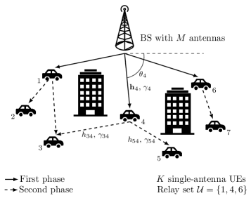
Figure 1: A BS equipped with $M$ antennas multicasts a common message to a subset of UEs with a properly designed precoding strategy in the first phase (solid lines). The UEs who successfully decode the message in the first phase retransmit it in the second phase to the remaining UEs via D2D links (dashed lines).

II-A Two-Phase Cooperative Multicasting

We consider a wireless network where a BS equipped with $M$ antennas aims at transmitting a common valuable message to a set of single-antenna UEs $\mathcal{K}\triangleq\{1,\ldots,K\}$, where $\mathbf{h}_{k}\in\mbox{$\mathbb{C}$}^{M\times 1}$ denotes the downlink channel between the BS and UE $k$. The UEs are also connected to each other via D2D links in half-duplex mode, where $h_{jk}\in\mbox{$\mathbb{C}$}$ denotes the D2D channel between UEs $j$ and $k$. We adopt a dense network scenario, i.e., where the number of receivers increases over a fixed network area, and we assume that $K\gg M$. For the sake of simplicity, we follow [5, 6] and focus on a cooperative scheme divided into two phases of equal length. Such a scheme is depicted in Fig. 1 and the two phases are described next.

• First phase. The BS transmits the message $\mathbf{x}\in\mbox{$\mathbb{C}$}^{M\times 1}$ at rate $r$, referred to as multicast rate, and with transmit covariance $\mathbf{\Gamma}\triangleq\mathbb{E}[\mathbf{x}\mathbf{x}^{\mathrm{H}}]$, with $\mathrm{tr}(\mathbf{\Gamma})\leq 1$. The receive signal at UE $k$ in the first phase is given by

  $$y_{k,1}\triangleq\sqrt{\xi_{0}}\mathbf{h}_{k}^{\mathrm{H}}\mathbf{x}+n_{k}\in\mbox{$\mathbb{C}$}$$ (1)

  where $\xi_{0}$ is the transmit power at the BS and, since we assume the additive white Gaussian noise (AWGN) noise term $n_{k}$ to be distributed as $\mathcal{CN}(0,1)$, it can be interpreted as the transmit signal-to-noise-ratio (SNR) at the BS. The message is decoded by UE $k$ if its achievable rate in the first phase is greater than or equal to the multicast rate $r$, i.e., if $\log_{2}(1+\xi_{0}\mathbf{h}_{k}^{\mathrm{H}}\mathbf{\Gamma}\mathbf{h}_{k})\geq r$. We define the subset of UEs whose achievable rate in the first phase is at least $r$ for a given transmit covariance as

  $$\mathcal{U}\triangleq\big{\{}k\in\mathcal{K}:\log_{2}(1+\xi_{0}\mathbf{h}_{k}^{\mathrm{H}}\mathbf{\Gamma}\mathbf{h}_{k})\geq r\big{\}}.$$ (2)

• Second phase. The UEs who were able to decode the message in the first phase jointly retransmit the message in an isotropic fashion, thus acting as opportunistic relays. Hence, the receive signal at UE $k$ in the second phase is a non-coherent sum of the D2D transmit signals and is given by

  $$y_{k,2}=\sum_{j\in\mathcal{U}}\sqrt{\xi_{j}}h_{jk}x_{j}+n_{k}\in\mbox{$\mathbb{C}$},\quad\forall k\in\mathcal{K}\setminus\mathcal{U}$$ (3)

  where $\xi_{j}$ is the transmit power at UE $j$ and can be interpreted as the transmit SNR at UE $j$ (cf. (1)); moreover, $x_{j}$ is the message transmitted by UE $j$, with $\mathbb{E}[|x_{j}|^{2}]=1$. The message is successfully decoded by UE $k$ if its achievable rate in the second phase is greater than or equal to $r$, i.e., if $\log_{2}\big{(}1+|\sum_{j\in\mathcal{U}}\sqrt{\xi_{j}}h_{jk}|^{2}\big{)}\geq r$.

II-B Single-Phase Multicasting

As a special case of the above, we describe a single-phase multicasting scheme, which we refer to as baseline scheme. This will serve as a means to assess the benefits brought by adding a second phase of D2D communications to traditional multi-antenna multicasting. In this scheme, the BS simply transmits the common message aiming at reaching all the UEs. The receive signal at UE $k$ is the same as (1) and the multicast capacity is given by (see [3])

$$C(\mathbf{H}) \triangleq\max_{\mathbf{\Gamma}\succeq\mathbf{0}\;:\;\mathrm{tr}(\mathbf{\Gamma})\leq 1}\min_{k\in\mathcal{K}}\log_{2}(1+\xi_{0}\mathbf{h}_{k}^{\mathrm{H}}\mathbf{\Gamma}\mathbf{h}_{k})$$ (4)

$$=\log_{2}\Big{(}1+\xi_{0}\max_{\mathbf{\Gamma}\succeq\mathbf{0}\;:\;\mathrm{tr}(\mathbf{\Gamma})\leq 1}\min_{k\in\mathcal{K}}\mathbf{h}_{k}^{\mathrm{H}}\mathbf{\Gamma}\mathbf{h}_{k}\Big{)}$$ (5)

where $\mathbf{H}=[\mathbf{h}_{1},\ldots,\mathbf{h}_{K}]\in\mbox{$\mathbb{C}$}^{M\times K}$. Although a closed-form expression of the multicast capacity is not available, $C(\mathbf{H})$ is convex in $\mathbf{\Gamma}$ and, therefore, it can be computed via semidefinite programming. The main drawback of this single-phase scheme is that the multicast capacity is limited by the UE with the worst channel conditions. In particular, for the case of i.i.d. Rayleigh fading channels and when the number of BS antennas $M$ is fixed, the multicast capacity scales as $K^{-1/M}$ [3].

II-C Channel Model

Following the millimeter wave (mmWave) one-ring channel model (see, e.g., [27] and references therein), let us express the direct channel to UE $k$ as

$$\mathbf{h}_{k}\triangleq\eta_{k}\sqrt{\gamma_{k}}\mathbf{a}_{k}\in\mbox{$\mathbb{C}$}^{M\times 1}$$ (6)

where $\eta_{k}\sim\mathcal{C}\mathcal{N}(0,1)$ is the small-scale fading coefficient, $\gamma_{k}$ is the average channel power gain, and $\mathbf{a}_{k}\in\mbox{$\mathbb{C}$}^{M\times 1}$ is the array response vector at the BS for the steering angle $\theta_{k}$, with $||\mathbf{a}_{k}||^{2}=M$. Here, we have $\gamma_{k}=d_{k}^{-\alpha}$ in case of line-of-sight (LoS) conditions and $\gamma_{k}=d_{k}^{-\beta}$ in case of non-line-of-sight (NLoS) conditions, where $d_{k}$ denotes the distance between the BS and UE $k$ and $\alpha$ (resp. $\beta$) is the LoS (resp. NLoS) pathloss exponent. For simplicity, we assume that the BS is equipped with a uniform linear array (ULA), such that

$$\mathbf{a}_{k}=[1,e^{-j2\pi\delta\cos(\theta_{k})},\ldots,e^{-j2\pi\delta(M-1)\cos(\theta_{k})}]^{\mathrm{T}}\in\mbox{$\mathbb{C}$}^{M\times 1}$$ (7)

where $\delta=0.5$ is the ratio between the antenna spacing and the signal wavelength. On the other hand, the D2D channel between UEs $k$ and $j$ is represented as

$$h_{jk}\triangleq\eta_{jk}\sqrt{\gamma_{jk}}\in\mbox{$\mathbb{C}$}$$ (8)

where $\eta_{kj}\sim\mathcal{CN}(0,1)$ is the small-scale fading coefficient and $\gamma_{jk}$ is the average channel power gain. Here, we have $\gamma_{jk}=d_{kj}^{-\alpha}$ in case of LoS conditions and $\gamma_{jk}=d_{kj}^{-\beta}$ in case of NLoS conditions, where $d_{jk}$ denotes the distance between UEs $k$ and $j$ (cf. (6)).

II-D CSIT Configurations

In this paper, we consider several configurations of CSIT that may be available at the BS under different application scenarios.

• Perfect CSITSection III. The knowledge of both the direct channels, i.e., $\{\mathbf{h}_{k}\}_{k\in\mathcal{K}}$, and the D2D channels, i.e., $\{h_{jk}\}_{k,j\in\mathcal{K}}$, is assumed.

• Statistical CSITSection IV. The knowledge of the UE locations is assumed. From this information, the BS can extract long-term statistics such as the average channel power gains of both the direct channels, i.e., $\{\gamma_{k}\}_{k\in\mathcal{K}}$, and the D2D channels, i.e., $\{\gamma_{jk}\}_{k,j\in\mathcal{K}}$, together with the steering angles $\{\theta_{k}\}_{k\in\mathcal{K}}$.

• Topological CSITSection V. The knowledge of the map of the network area, i.e., the location and size of the obstacles (such as buildings) within its coverage area, and of the pdf of the UE locations is assumed.

The above configurations correspond to settings with decreasing requirements on the information available at the BS. While configuration i) is relevant for the case of moderate (or finite) number of UEs and low mobility, configuration iii) is relevant for the case of large number of UE and high mobility: for instance, these features arise in vehicular networks, where the BS multi-antenna beam pattern ought to be designed on the basis of a city map and road traffic distribution. Lastly, configuration ii) can be considered as an intermediate case between i) and iii).

II-E Performance Metrics

We propose two different performance metrics in terms of service reliability. In order to reflect the inherent difficulty to guarantee a given data rate in a wireless setting with uncertainties on the channel conditions across the UEs, we introduce the target outage $\epsilon\in[0,1)$, which describes the trade-off between the multicast rate and the reliability level at which we can maintain such a rate. Furthermore, let $\mathrm{P}_{k,1}(r,\mathbf{\Gamma})$ and $\mathrm{P}_{k,2}(r,\mathbf{\Gamma})$ denote the probabilities that UE $k$ successfully decodes in the first and in the second phase, respectively.

• Average multicast rate. We define the average success probability as the probability that a randomly chosen UE successfully decodes over the two phases, which is given by

  $$\mathrm{P}_{\mathrm{A}}(r,\mathbf{\Gamma})\triangleq\frac{1}{K}\sum_{k\in\mathcal{K}}\big{[}\mathrm{P}_{k,1}(r,\mathbf{\Gamma})+\big{(}1-\mathrm{P}_{k,1}(r,\mathbf{\Gamma})\big{)}\mathrm{P}_{k,2}(r,\mathbf{\Gamma})\big{]}.$$ (9)

  Hence, the average multicast rate is defined as the maximum transmission rate at which a randomly chosen UE successfully decodes with probability at least $1-\epsilon$ over the two phases, which can be expressed as

  $$\mathrm{R}_{\mathrm{A}}(r,\mathbf{\Gamma})\triangleq\frac{1}{2}r\quad\textrm{with}~{}r~{}\textrm{solution to}~{}\mathrm{P}_{\mathrm{A}}(r,\mathbf{\Gamma})\geq 1-\epsilon.$$ (10)

• Outage multicast rate. Let us introduce the binary variables $z_{k,1}(r,\mathbf{\Gamma})$ and $z_{k,2}(r,\mathbf{\Gamma})$, which are equal to $1$ if UE $k$ successfully decodes in the first and in the second phase, respectively, and to $0$ otherwise. Furthermore, let $\mathbf{z}_{1}(r,\mathbf{\Gamma})\triangleq[z_{1,1}(r,\mathbf{\Gamma})\ldots z_{K,1}(r,\mathbf{\Gamma})]$. We define the joint success probability as the probability that all the UEs successfully decode over the two phases, which is given by

  $$\mathrm{P}_{\mathrm{J}}(r,\mathbf{\Gamma})\triangleq\mathbb{E}\bigg{[}\prod_{k\in\mathcal{K}}\mathbb{P}\bigg{[}\log_{2}\bigg{(}1+\bigg{\rvert}\sum_{j\neq k}\xi_{j}h_{kj}\bigg{\rvert}^{2}\bigg{)}\geq r\big{(}1-z_{k,1}(r,\mathbf{\Gamma})\big{)}\bigg{\rvert}\mathbf{z}_{1}(r,\mathbf{\Gamma})\bigg{]}\bigg{]}.$$ (11)

  Hence, the outage multicast rate is defined as the maximum transmission rate at which all the UEs successfully decode with probability at least $1-\epsilon$ over the two phases, which can be expressed as

  $$\mathrm{R}_{\mathrm{O}}(r,\mathbf{\Gamma})\triangleq\frac{1}{2}r\quad\textrm{with}~{}r~{}\textrm{solution to}~{}\mathrm{P}_{\mathrm{J}}(r,\mathbf{\Gamma})\geq 1-\epsilon.$$ (12)

II-F Problem Formulation

Our objective is to jointly optimize the multicast rate $r$ and the transmit covariance $\mathbf{\Gamma}$ under one of the above outage constraints over the two phases. Such a problem can be formalized as

$$\begin{array}[]{cl}\displaystyle\max_{r>0,\mathbf{\Gamma}\succeq\mathbf{0}}&\displaystyle\frac{1}{2}r\\ \mathrm{s.t.}&\mathrm{tr}(\mathbf{\Gamma})\leq 1,\\ &\mathrm{P}_{\mathrm{T}}(r,\mathbf{\Gamma})\geq 1-\epsilon\end{array}$$ (16)

where $\mathrm{T}\in\{\mathrm{A},\mathrm{J}\}$. Hence, when $\mathrm{T}=\mathrm{A}$, we recover the average multicast rate $\mathrm{R}_{\mathrm{A}}(r,\mathbf{\Gamma})$ defined in (10) and, when $\mathrm{T}=\mathrm{J}$, we recover the outage multicast rate $\mathrm{R}_{\mathrm{O}}(r,\mathbf{\Gamma})$ defined in (12). Note that problem (16) is non-convex in both optimization variables due to the non-convex outage constraint and is thus highly complex to solve. In the following, we detail our proposed methods to tackle problem (16) in the three CSIT configurations described in Section II-D.

III D2D-Aided Multi-Antenna Multicasting with Perfect CSIT

In this section, we consider the case where all the direct channels, i.e., $\{\mathbf{h}_{k}\}_{k\in\mathcal{K}}$, and all the D2D channels, i.e., $\{h_{jk}\}_{k,j\in\mathcal{K}}$, are perfectly known at the BS. For each UE $k$, let us define the binary variables

$$z_{k,1}(r,\mathbf{\Gamma}) \triangleq\mathbbm{1}\big{[}\log_{2}(1+\xi_{0}\mathbf{h}_{k}^{\mathrm{H}}\mathbf{\Gamma}\mathbf{h}_{k})\geq r\big{]},$$ (17)

$$z_{k,2}(r,\mathbf{\Gamma}) \triangleq\mathbbm{1}\bigg{[}\log_{2}\bigg{(}1+\bigg{|}\sum_{j\in\mathcal{K}\setminus\{k\}}z_{j,1}(r,\mathbf{\Gamma})\sqrt{\xi_{j}}h_{jk}\bigg{|}^{2}\bigg{)}\geq r\bigg{]}$$ (18)

which are equal to $1$ if the UE successfully decodes in the first and in the second phase, respectively, and to $0$ otherwise. Hence, the probabilities that UE $k$ successfully decodes in the first and in the second phase are given by

$$\mathrm{P}_{k,1}(r,\mathbf{\Gamma})=z_{k,1}(r,\mathbf{\Gamma}),$$ (19)

$$\mathrm{P}_{k,2}(r,\mathbf{\Gamma})=z_{k,2}(r,\mathbf{\Gamma})$$ (20)

respectively: these stem from the fact that, with perfect CSIT, the decodability of each UE in each phase is deterministic. In this context, the average success probability in (9) can be written as

$$\mathrm{P}_{\mathrm{A}}(r,\mathbf{\Gamma})=\frac{1}{K}\sum_{k\in\mathcal{K}}\big{(}z_{k,1}(r,\mathbf{\Gamma})+\big{(}1-z_{k,1}(r,\mathbf{\Gamma})\big{)}z_{k,2}(r,\mathbf{\Gamma})\big{)}.$$ (21)

On the other hand, the joint success probability in (11) becomes a product of binary variables, which is equal to $0$ if even a single UE does not decode the message over the two phases: hence, it is not suited to accommodate any target outage in the case of perfect CSIT. For this reason, in the rest of the section, we focus on maximizing the average multicast rate in (10).

III-A Multi-Antenna Multicasting (MAM) Algorithm

Considering the single-phase baseline scheme described in Section II-B, problem (16) with $\mathrm{T}=\mathrm{A}$ and perfect CSIT can be solved by selecting the best subset of $\mathcal{K}$ with size $(1-\epsilon)K$ to be served by the BS and computing the transmit covariance that maximizes the multicast rate over such a subset of UEs. Note that, in this case, the outage constraint in (16) can be simply expressed as $\sum_{k\in\mathcal{K}}z_{k,1}(r,\mathbf{\Gamma})\geq(1-\epsilon)K$. While this problem formulation is also novel, it mainly serves as a benchmark to demonstrate the gains obtained by the adding a second phase of UE cooperation enabled by D2D links in Section VI. However, the problem of deriving the optimal UE selection strategy is NP-hard since it requires to evaluate all possible subsets of $\mathcal{K}$ with size $(1-\epsilon)K$. To reduce the complexity, we build on the intuition described in the following lemma to derive a suboptimal UE selection scheme.

Lemma 1.

For a class of channels satisfying $\mathbb{E}[\mathbf{h}_{k}\mathbf{h}_{k}^{\mathrm{H}}]=\gamma_{k}\mathbf{I}_{M}$, $\forall k\in\mathcal{K}$, which includes (6), the optimal UE selection strategy with statistical channel knowledge is the one choosing the $(1-\epsilon)K$ UEs with the highest average channel power gains among $\{\gamma_{k}\}_{k\in\mathcal{K}}$.

Proof:

If $\{\gamma_{k}>0\}_{k\in\mathcal{K}}$ are known at the BS, we have

$$\max_{\mathcal{U}\subset\mathcal{K}\;:\;|\mathcal{U}|=(1-\epsilon)K}\mathbb{E}\Big{[}\max_{\mathbf{\Gamma}\succeq\mathbf{0}\;:\;\mathrm{tr}(\mathbf{\Gamma})\leq 1}\min_{k\in\mathcal{U}}\mathbf{h}_{k}^{\mathrm{H}}\mathbf{\Gamma}\mathbf{h}_{k}\Big{]}$$

$$\leq\max_{\mathcal{U}\subset\mathcal{K}\;:\;|\mathcal{U}|=(1-\epsilon)K}\;\max_{\mathbf{\Gamma}\succeq\mathbf{0}\;:\;\mathrm{tr}(\mathbf{\Gamma})\leq 1}\min_{k\in\mathcal{U}}\mathbb{E}[\mathbf{h}_{k}^{\mathrm{H}}\mathbf{\Gamma}\mathbf{h}_{k}]$$ (22)

$$=\max_{\mathcal{U}\subset\mathcal{K}\;:\;|\mathcal{U}|=(1-\epsilon)K}\;\max_{\mathbf{\Gamma}\succeq\mathbf{0}\;:\;\mathrm{tr}(\mathbf{\Gamma})\leq 1}\min_{k\in\mathcal{U}}\mathrm{tr}\big{(}\mathbf{\Gamma}\mathbb{E}[\mathbf{h}_{k}\mathbf{h}_{k}^{\mathrm{H}}]\big{)}$$ (23)

$$=\max_{\mathcal{U}\subset\mathcal{K}\;:\;|\mathcal{U}|=(1-\epsilon)K}\min_{k\in\mathcal{U}}\gamma_{k}$$ (24)

where (22) follows from the concavity of $\min_{k\in\mathcal{U}}\mathbf{h}_{k}^{\mathrm{H}}\mathbf{\Gamma}\mathbf{h}_{k}$ and (24) is due to the fact that the optimal $\mathbf{\Gamma}$ satisfies $\mathrm{tr}(\mathbf{\Gamma})=1$. Finally, the solution presented in the lemma readily follows from (24). ∎

Lemma 1 states that, if the channels can be ordered statistically based on the average channel power gains $\{\gamma_{k}\}_{k\in\mathcal{K}}$, the exhaustive search over all possible subsets of $\mathcal{K}$ with size $(1-\epsilon)K$ reduces to choosing the $(1-\epsilon)K$ UEs with the highest $\gamma_{k}$. Motivated by this observation, we thus propose to apply such a UE selection strategy to the case of perfect CSIT and obtain the multi-antenna multicasting (MAM) algorithm. More specifically, we build $\mathcal{U}\subset\mathcal{K}$ by selecting the $(1-\epsilon)K$ UEs with the highest channel power gain $\|\mathbf{h}_{k}\|^{2}$ and compute the transmit covariance that achieves the multicast capacity over $\mathcal{U}$, i.e.,

$$\mathbf{\Gamma}_{1}=\operatornamewithlimits{argmax}_{\mathbf{\Gamma}\succeq\mathbf{0}\;:\;\mathrm{tr}(\mathbf{\Gamma})\leq 1}\min_{k\in\mathcal{U}}\mathbf{h}_{k}^{\mathrm{H}}\mathbf{\Gamma}\mathbf{h}_{k}.$$ (25)

Since the whole time resource is dedicated to the first phase, the resulting average multicast rate is given by

$$r_{1}=\log_{2}\Big{(}1+\xi_{0}\min_{k\in\mathcal{U}}\mathbf{h}_{k}^{\mathrm{H}}\mathbf{\Gamma}_{1}\mathbf{h}_{k}\Big{)}.$$ (26)

III-B D2D-Aided Multi-Antenna Multicasting (D2D-MAM) Algorithm

To solve problem (16) with $\mathrm{T}=\mathrm{A}$ and perfect CSIT, we resort to the alternating optimization of the multicast rate $r$ and the transmit covariance $\mathbf{\Gamma}$. In this respect, we propose an efficient iterative algorithm whose goal is to serve a subset of UEs (which are suitably selected by means of precoding at the BS) in the first phase such that the multicast rate is maximized. At each iteration $n$, the transmit covariance $\mathbf{\Gamma}^{(n)}$ that achieves the multicast capacity over a predetermined subset $\mathcal{U}^{(n-1)}\subset\mathcal{K}$ is computed (see (4)–(5)). Then, the multicast rate $r^{(n)}$ is obtained as the maximum rate that guarantees the outage constraint over the two phases given the transmit covariance computed in the previous step, i.e., such that $\mathrm{P}_{\mathrm{A}}(r^{(n)},\mathbf{\Gamma}^{(n)})\geq 1-\epsilon$. The new $r^{(n)}$ yields an updated $\mathcal{U}^{(n)}$ of UEs that are able to decode in the first phase and, therefore, an improved transmit covariance can be obtained by optimizing over $\mathcal{U}^{(n)}$. This procedure is iterated until the multicast rate converges. The proposed algorithm is referred to as D2D-aided multi-antenna multicasting (D2D-MAM) algorithm and is formally described in Algorithm 1. The D2D-MAM algorithm has the key advantage of not requiring any tuning parameter selection. Furthermore, it converges to a local optimum of problem (16) with $\mathrm{T}=\mathrm{A}$, as formalized in the following theorem.

   Data: Direct channels $\{\mathbf{h}_{k}\}_{k\in\mathcal{K}}$ and D2D channels $\{h_{jk}\}_{k,j\in\mathcal{K}}$. Fix $\mathcal{U}^{(0)}=\mathcal{K}$ and $n=1$.

• Optimize the transmit covariance as

  $$\mathbf{\Gamma}^{(n)}=\operatornamewithlimits{argmax}_{\mathbf{\Gamma}\succeq\mathbf{0}\;:\;\mathrm{tr}(\mathbf{\Gamma})\leq 1}\min_{k\in\mathcal{U}^{(n-1)}}\mathbf{h}_{k}^{\mathrm{H}}\mathbf{\Gamma}\mathbf{h}_{k}.$$

• Maximize the multicast rate as

  $$r^{(n)}=\max\big{\{}r:\mathrm{P}_{\mathrm{A}}(r,\mathbf{\Gamma}^{(n)})=1-\epsilon\big{\}}.$$

• Update the subset of UEs successfully decoding in the first phase as

  $$\mathcal{U}^{(n)}=\big{\{}k:\log_{2}(1+\xi_{0}\mathbf{h}_{k}^{\mathrm{H}}\mathbf{\Gamma}^{(n)}\mathbf{h}_{k})\geq r^{(n)}\big{\}}.$$

• If $r^{(n)}=r^{(n-1)}$: fix $\mathbf{\Gamma}=\mathbf{\Gamma}^{(n)}$ and $r=r^{(n)}$; Stop.

• Else: $n\leftarrow n+1$; Go to (S.1).

Algorithm 1 (D2D-MAM)

Theorem 1.

The D2D-MAM algorithm converges to a local optimum of problem (16) with $\mathrm{T}=\mathrm{A}$.

Proof:

Since step (S.1) of Algorithm 1 optimizes $\mathbf{\Gamma}^{(n)}$ over $\mathcal{U}^{(n-1)}$, we have

$$\min_{k\in\mathcal{U}^{(n-1)}}\mathbf{h}_{k}^{\mathrm{H}}\mathbf{\Gamma}^{(n)}\mathbf{h}_{k}\geq\min_{k\in\mathcal{U}^{(n-1)}}\mathbf{h}_{k}^{\mathrm{H}}\mathbf{\Gamma}^{(n-1)}\mathbf{h}_{k}$$ (27)

i.e., the minimum rate achievable by the UEs in $\mathcal{U}^{(n-1)}$ increases with the new transmit covariance $\mathbf{\Gamma}^{(n)}$. Furthermore, at each iteration $n$ of the D2D-MAM algorithm, the following holds:

$$r^{(n)} \geq\log_{2}\Big{(}1+\rho\min_{k\in\mathcal{U}^{(n-1)}}\mathbf{h}_{k}^{\mathrm{H}}\mathbf{\Gamma}^{(n)}\mathbf{h}_{k}\Big{)}$$ (28)

$$\geq\log_{2}\Big{(}1+\rho\min_{k\in\mathcal{U}^{(n-1)}}\mathbf{h}_{k}^{\mathrm{H}}\mathbf{\Gamma}^{(n-1)}\mathbf{h}_{k}\Big{)}$$ (29)

$$\geq r^{(n-1)}$$ (30)

where (28) follows from step (S.2) of Algorithm 1 (by which it is possible to increase the multicast rate as long as the outage constraint is guaranteed), (29) is a direct consequence of (27), and (30) stems from the fact that $\mathcal{U}^{(n-1)}$ contains the UEs whose achievable rate in the first phase is at least $r^{(n-1)}$. Hence, the multicast rate cannot decrease between consecutive iterations. Finally, if $\mathcal{U}^{(n)}=\mathcal{U}^{(n-1)}$, then it is not possible to further increase the multicast rate, i.e., $r^{(n)}=r^{(n-1)}$, which implies that convergence is reached. ∎

Regarding the optimization of the multicast rate in step (S.2) of Algorithm 1, we have

$$r^{(n)}\in\Big{[}r^{(n-1)},\log_{2}\Big{(}1+\rho\max_{k\in\mathcal{U}^{(n-1)}}\mathbf{h}_{k}^{\mathrm{H}}\mathbf{\Gamma}^{(n)}\mathbf{h}_{k}\Big{)}\Big{]}$$ (31)

where the lower bound follows from Theorem 1 and the upper bound is necessary to guarantee that at least one UE is served in the first phase: thus, $r^{(n)}$ can be efficiently computed by means of bisection over the above interval. Accordingly, every iteration of the D2D-MAM algorithm requires the solution of a convex problem in step (S.1) and a linear search in step (S.2); in addition, for the settings considered for our simulations in Section VI, convergence is reached after a small number of iterations. Hence, the D2D-MAM algorithm provides a locally optimal solution of problem (16) with $\mathrm{T}=\mathrm{A}$ with very low complexity.

IV D2D-Aided Multi-Antenna Multicasting with Statistical CSIT

In this section, we consider the case where only the UE locations are known at the BS. From this information, the BS can extract long-term statistics such as the average channel power gains of both the direct channels, i.e., $\{\gamma_{k}\}_{k\in\mathcal{K}}$, and the D2D channels, i.e., $\{\gamma_{jk}\}_{k,j\in\mathcal{K}}$, together with the steering angles $\{\theta_{k}\}_{k\in\mathcal{K}}$. On the other hand, the BS has no knowledge of the small-scale fading coefficients, i.e., $\{\eta_{k}\}_{k\in\mathcal{K}}$ and $\{\eta_{jk}\}_{k,j\in\mathcal{K}}$. Under statistical CSIT, we characterize the service reliability in terms of the joint success probability in (11) and, accordingly, we maximize the outage multicast rate in (12). To alleviate the task of dealing with the involved expression of the joint success probability, we derive its deterministic equivalent in the following proposition.

Proposition 1.

Assuming that all (direct and D2D) channels are independent, we have

$$\mathrm{P}_{\mathrm{J}}(r,\mathbf{\Gamma})\underset{K\to\infty}{\overset{\mathbb{P}}{\to}}\bar{\mathrm{P}}_{\mathrm{J}}(r,\mathbf{\Gamma})$$ (32)

where

$$\bar{\mathrm{P}}_{\mathrm{J}}(r,\mathbf{\Gamma}) \triangleq\mathrm{exp}\bigg{(}-\sum_{k\in\mathcal{K}}\frac{(2^{r}-1)\big{(}1-\mathrm{P}_{k,1}(r,\mathbf{\Gamma})\big{)}}{\sum_{j\in\mathcal{K}\setminus\{k\}}\mathrm{P}_{j,1}(r,\mathbf{\Gamma})\gamma_{jk}\xi_{j}}\bigg{)}$$ (33)

is the deterministic equivalent of $\mathrm{P}_{\mathrm{J}}(r,\mathbf{\Gamma})$ in (11).

Proof:

The proof follows similar steps as the proof of [18, Thm. 4] and is thus omitted. ∎

Note that, with statistical CSIT, the probability that UE $k$ successfully decodes in the first phase is given by

$$\mathrm{P}_{k,1}(r,\mathbf{\Gamma}) =\mathbb{P}\big{[}z_{k,1}(r,\mathbf{\Gamma})=1\big{]}$$ (34)

$$=\mathbb{P}\big{[}\log_{2}(1+\xi_{0}\gamma_{k}|\eta_{k}|^{2}\mathbf{a}^{\mathrm{H}}_{k}\mathbf{\Gamma}\mathbf{a}_{k})\geq r\big{]}$$ (35)

$$=\exp\bigg{(}-\frac{2^{r}-1}{\xi_{0}\gamma_{k}\mathbf{a}^{\mathrm{H}}_{k}\mathbf{\Gamma}\mathbf{a}_{k}}\bigg{)}.$$ (36)

with $z_{k,1}(r,\mathbf{\Gamma})$ defined in (17) and where (36) follows from the exponential distribution of $|\eta_{k}|^{2}$. In the rest of the section, we replace $\mathrm{P}_{\mathrm{J}}(r,\mathbf{\Gamma})$ with its deterministic equivalent $\bar{\mathrm{P}}_{\mathrm{J}}(r,\mathbf{\Gamma})$ in (33).

IV-A Statistical Multi-Antenna Multicasting (SMAM) Algorithm

Considering the single-phase baseline scheme described in Section II-B, problem (16) with $\mathrm{T}=\mathrm{J}$ and statistical CSIT can be solved by computing the transmit covariance that maximizes the outage multicast rate. Note that, in this case, the outage constraint in (16) can be simply expressed as $\prod_{k\in\mathcal{K}}\mathrm{P}_{k,1}(r,\mathbf{\Gamma})\geq 1-\epsilon$. Since this problem is convex in $\mathbf{\Gamma}$ for a fixed $r$ and vice versa, we decouple the optimization over the two variables in the following way. For a given transmit covariance $\mathbf{\Gamma}_{1}$, the outage multicast rate, denoted in this context by $R_{\mathrm{O},1}(r_{1},\mathbf{\Gamma}_{1})$, is maximized when the outage constraint is satisfied with equality, leading to

$$R_{\mathrm{O},1}(r_{1},\mathbf{\Gamma}_{1})=\log_{2}\bigg{(}1+\xi_{0}\log\bigg{(}\frac{1}{1-\epsilon}\bigg{)}\bigg{(}\sum_{k\in\mathcal{K}}\frac{1}{\gamma_{k}\mathbf{a}_{k}^{\mathrm{H}}\mathbf{\Gamma}_{1}\mathbf{a}_{k}}\bigg{)}^{-1}\bigg{)}.$$ (37)

Then, the optimal transmit covariance is obtained by solving

$$\begin{array}[]{cl}\displaystyle\min_{\mathbf{\Gamma}_{1}\succeq\mathbf{0}}&\displaystyle\sum_{k\in\mathcal{K}}\frac{1}{\gamma_{k}\mathbf{a}_{k}^{\mathrm{H}}\mathbf{\Gamma}_{1}\mathbf{a}_{k}}\\ \mathrm{s.t.}&\mathrm{tr}(\mathbf{\Gamma}_{1})\leq 1\end{array}$$ (40)

by means of semidefinite programming. As in Section III-A, this problem formulation mainly serves for the comparative purposes in Section VI. The resulting algorithm is referred to as statistical multi-antenna multicasting (SMAM) algorithm.

The following proposition derives a tractable expression of $\mathbf{\Gamma}_{1}$ and will be useful in the next section.

Proposition 2.

Assume that $\mathcal{K}$ consists of $M$ UEs exhibiting mutually orthogonal array responses, i.e.,

$$\sum_{k\in\mathcal{K}}\mathbf{a}_{k}\mathbf{a}_{k}^{\mathrm{H}}=M\mathbf{I}_{M}.$$ (41)

Then, the optimal transmit covariance for problem (40) can be written in closed form as

$$\mathbf{\Gamma}_{1}=\frac{1}{M\nu_{\mathcal{K}}}\sum_{k\in\mathcal{K}}\frac{1}{\sqrt{\gamma_{k}}}\mathbf{a}_{k}\mathbf{a}_{k}^{\mathrm{H}}$$ (42)

with $\nu_{\mathcal{K}}\triangleq\sum_{k\in\mathcal{K}}\frac{1}{\sqrt{\gamma_{k}}}$.

Proof:

See Appendix A. ∎

A set of array response vectors satisfying (41) can be obtained as the columns of the $M$-dimensional discrete Fourier transform (DFT) matrix or, alternatively, it can be constructed along specific virtual angles as described in [28].

IV-B D2D-Aided Statistical Multi-Antenna Multicasting (D2D-SMAM) Algorithm

To solve problem (16) with $\mathrm{T}=\mathrm{J}$ and statistical CSIT, we use the deterministic equivalent derived in Proposition 1 and, to further reduce the complexity, we decouple the optimization across the two phases in the following way. First, we carefully select a subset $\mathcal{U}\subset\mathcal{K}$ of UEs with favorable statistical properties to be served in the first phase by the BS. In particular, assuming large $K$ and uniform UE distribution in the angular domain, we build on Proposition 2 and construct $\mathcal{U}$ by selecting $M$ UEs satisfying the condition in (41): by doing so, the BS spreads its transmit power along a set of orthogonal directions spanning the whole angular domain. In this setting, the transmit covariance that maximizes the multicast rate over $\mathcal{U}$ is given by $\mathbf{\Gamma}_{1}$ in (42). Next, we fix the joint success probability in the first phase over $\mathcal{U}$ to a given value $1-\epsilon_{1}$ and obtain the corresponding multicast rate $r(\epsilon_{1})$ from (37). Finally, we optimize $\epsilon_{1}$ in order to obtain the desired joint success probability $1-\epsilon$ over the two phases.

Let us first focus on maximizing the outage multicast rate over $\mathcal{U}$ in the first phase, i.e.,

$$\begin{array}[]{cl}\displaystyle\max_{r(\epsilon_{1})>0,\mathbf{\Gamma}\succeq\mathbf{0}}&\displaystyle r(\epsilon_{1})\\ \mathrm{s.t.}&\mathrm{tr}(\mathbf{\Gamma})\leq 1,\\ &\displaystyle\exp\bigg{(}-\sum_{k\in\mathcal{U}}\frac{2^{r(\epsilon_{1})}-1}{\xi_{0}\gamma_{k}\mathbf{a}^{\mathrm{H}}_{k}\mathbf{\Gamma}\mathbf{a}_{k}}\bigg{)}\geq 1-\epsilon_{1}.\end{array}$$ (46)

Since the outage constraint is convex in $\mathbf{\Gamma}$, we can solve problem (46) by decoupling the optimization of $r(\epsilon_{1})$ and $\mathbf{\Gamma}$. Letting the outage constraint be satisfied with equality, we have that the multicast rate becomes

$$r(\epsilon_{1})=\log_{2}\bigg{(}1+\xi_{0}\log\bigg{(}\frac{1}{1-\epsilon_{1}}\bigg{)}\bigg{(}\sum_{k\in\mathcal{U}}\frac{1}{\gamma_{k}\mathbf{a}^{\mathrm{H}}_{k}\mathbf{\Gamma}\mathbf{a}_{k}}\bigg{)}^{-1}\bigg{)}$$ (47)

and problem (46) reduces to finding the transmit covariance $\mathbf{\Gamma}$ by solving

$$\begin{array}[]{cl}\displaystyle\min_{\mathbf{\Gamma}\succeq\mathbf{0}}&\displaystyle\sum_{k\in\mathcal{U}}\frac{1}{\gamma_{k}\mathbf{a}_{k}^{\mathrm{H}}\mathbf{\Gamma}\mathbf{a}_{k}}\\ \mathrm{s.t.}&\mathrm{tr}(\mathbf{\Gamma})\leq 1.\end{array}$$ (50)

From Proposition 2, the transmit covariance resulting from the above problem is known to have a simple closed-form expression when $|\mathcal{U}|=M$ and the UEs in $\mathcal{U}$ exhibit orthogonal array response vectors, i.e.,

$$\sum_{k\in\mathcal{U}}\mathbf{a}_{k}\mathbf{a}_{k}^{\mathrm{H}}=M\mathbf{I}_{M}.$$ (51)

Since $K$ is large, we assume that it is always possible to build $\mathcal{U}$ by selecting $M$ UEs satisfying the condition in (51). In this case, the optimal transmit covariance is given by

$$\mathbf{\Gamma}=\sum_{j\in\mathcal{U}}w_{j}\mathbf{a}_{j}\mathbf{a}_{j}^{\mathrm{H}}$$ (52)

with weights given by

$$w_{j}\triangleq\frac{1}{M\bar{\gamma}_{\mathcal{U}}}\frac{1}{\sqrt{\gamma_{j}}}\quad\forall j\in\mathcal{U}$$ (53)

and where we have defined $\bar{\gamma}_{\mathcal{U}}\triangleq\sum_{k\in\mathcal{U}}\frac{1}{\sqrt{\gamma_{k}}}$. Finally, plugging (52) and (53) into (47), we obtain

$$r(\epsilon_{1}) =\log_{2}\bigg{(}1+\xi_{0}\log\bigg{(}\frac{1}{1-\epsilon_{1}}\bigg{)}\frac{M}{\bar{\gamma_{\mathcal{U}}}^{2}}\bigg{)}.$$ (54)

Let us now focus on deriving $\epsilon_{1}$ that achieves the desired joint success probability $1-\epsilon$ over the two phases. This can be done by solving the following expression for $\epsilon_{1}\in[0,1)$ (e.g., by means of bisection):

$$(2^{r(\epsilon_{1})}-1)\sum_{k\in\mathcal{K}}\frac{1-\mathrm{exp}\big{(}-\frac{2^{r(\epsilon_{1})}-1}{\xi_{0}\gamma_{k}\mathbf{a}_{k}^{\mathrm{H}}\mathbf{\Gamma}\mathbf{a}_{k}}\big{)}}{\sum_{j\in\mathcal{K}\setminus\{k\}}\mathrm{exp}\big{(}-\frac{2^{r(\epsilon_{1})}-1}{\xi_{0}\gamma_{k}\mathbf{a}_{k}^{\mathrm{H}}\mathbf{\Gamma}\mathbf{a}_{k}}\big{)}\gamma_{jk}\xi_{j}}\leq\log\bigg{(}\frac{1}{1-\epsilon}\bigg{)}.$$ (55)

The proposed algorithm is referred to as D2D-aided statistical multi-antenna multicasting (D2D-SMAM) algorithm and is formally described in Algorithm 2. In the next section, we illustrate a possible way to derive an approximation of the optimal $\epsilon_{1}$.

   Data: Build $\mathcal{U}$ by selecting $M$ UEs such that (51) holds.

• Compute the transmit covariance as in (52) with weights given in (53).

• Find $\epsilon_{1}$ by solving (55).

• Compute the multicast rate as in (54).

Algorithm 2 (D2D-SMAM)

IV-C Asymptotic Behavior of the D2D-SMAM Algorithm

Let us assume that $\epsilon\to 0$ and, consequently, that $\epsilon_{1}\to 0$. By applying the Taylor approximation $\mathrm{exp}\left(-\frac{2^{r(\epsilon_{1})-1}}{\xi_{0}\gamma_{k}\mathbf{a}_{k}^{\mathrm{H}}\mathbf{\Gamma}\mathbf{a}_{k}}\right)\approx 1-\frac{2^{r(\epsilon_{1})-1}}{\xi_{0}\gamma_{k}\mathbf{a}_{k}^{\mathrm{H}}\mathbf{\Gamma}\mathbf{a}_{k}}$ to (55), we have

$$\epsilon_{1}\underset{\epsilon\to 0}{\sim}1-\mathrm{exp}\Bigg{(}-\frac{\bar{\gamma}_{\mathcal{U}}^{2}}{M\xi_{0}}\sqrt{\frac{\log\big{(}\frac{1}{1-\epsilon}\big{)}}{\sum_{k\in\mathcal{K}}\frac{1}{\xi_{0}\gamma_{k}\mathbf{a}_{k}^{\mathrm{H}}\mathbf{\Gamma}\mathbf{a}_{k}}\big{(}\sum_{j\in\mathcal{K}\setminus\{k\}}\gamma_{jk}\xi_{j}\big{)}^{-1}}}\Bigg{)}$$ (56)

and, hence

$$r \underset{\epsilon\to 0}{\sim}\frac{1}{2}\log_{2}\Bigg{(}1+\sqrt{\frac{\xi_{0}\log\big{(}\frac{1}{1-\epsilon}\big{)}}{\sum_{k\in\mathcal{K}}\frac{1}{\gamma_{k}\mathbf{a}_{k}^{\mathrm{H}}\mathbf{\Gamma}\mathbf{a}_{k}}\big{(}\sum_{j\in\mathcal{K}\setminus\{k\}}\gamma_{jk}\xi_{j}\big{)}^{-1}}}\Bigg{)}$$ (57)

$$\ \triangleq\ \tilde{r}.$$ (58)

Now, assume that $d_{k}\in[R_{\min},R_{\max}]$, $\forall k\in\mathcal{K}$, where $R_{\min}$ and $R_{\max}$ denote the minimum and maximum distance, respectively, between each UE and the BS. It follows that the average channel power gains can be bounded as

$$\gamma_{k} \in[R_{\max}^{-\beta},R_{\min}^{-\alpha}],\hskip 68.8556pt\forall k\in\mathcal{K},$$ (59)

$$\gamma_{jk} \in\big{[}(2R_{\max})^{-\beta},(2R_{\min})^{-\alpha}],\quad\forall k,j\in\mathcal{K}.$$ (60)

In this setting, we have

$$\mathbf{a}_{k}^{\mathrm{H}}\mathbf{\Gamma}\mathbf{a}_{k} =\frac{1}{M\bar{\gamma}_{\mathcal{U}}}\sum_{j\in\mathcal{U}}\frac{1}{\sqrt{\gamma_{j}}}|\mathbf{a}_{k}^{\mathrm{H}}\mathbf{a}_{j}|^{2}$$ (61)

$$\geq\frac{M}{\bar{\gamma}_{\mathcal{U}}}R_{\min}^{\alpha/2}$$ (62)

where (62) follows from assuming that all the UEs in $\mathcal{U}$ are at distance $R_{\min}$ from the BS, i.e., $\{\gamma_{j}=R_{\min}^{-\alpha}\}_{j\in\mathcal{U}}$. Hence, we have that $\tilde{r}$ defined in (57)–(58) can be lower bounded as

$$\tilde{r}\geq\log_{2}\Bigg{(}1+\sqrt{\frac{\xi_{0}\xi_{\textnormal{\tiny{UE}}}(K-1)M\log\big{(}\frac{1}{1-\epsilon}\big{)}R_{\mathrm{min}}^{\alpha/2}}{\bar{\gamma}_{\mathcal{U}}^{2}(2R_{\mathrm{max}})^{\beta}R_{\mathrm{min}}^{\alpha/2}+2^{\beta}\bar{\gamma}_{\mathcal{U}}R_{\mathrm{max}}^{2\beta}(K-M)}}\Bigg{)}$$ (63)

where, for simplicity, we have assumed that $\{\xi_{k}=\xi_{\textnormal{\tiny{UE}}}\}_{k\in\mathcal{K}}$ (i.e., all the UEs have the same transmit SNR in the second phase). Finally, we consider the asymptotic behavior of $\tilde{r}$ in the case where both $K$ and $M$ increase with fixed ratio $c\triangleq\frac{K}{M}>1$ as well as in the case where $K$ increases for a fixed $M$. Hence, (63) behaves as

$$\tilde{r}\underset{K\to\infty}{\to}\begin{cases}\log_{2}\bigg{(}1+\sqrt{\frac{\xi_{0}\xi_{\textnormal{\tiny{UE}}}M\log\big{(}\frac{1}{1-\epsilon}\big{)}R_{\mathrm{min}}^{\alpha/2}}{2^{\beta}\bar{\gamma}_{\mathcal{U}}R_{\mathrm{max}}^{2\beta}}}\bigg{)}&\textrm{for fixed}~{}M\\ \log_{2}\bigg{(}1+\sqrt{\frac{\xi_{0}\xi_{\textnormal{\tiny{UE}}}\log\big{(}\frac{1}{1-\epsilon}\big{)}R_{\mathrm{min}}^{\alpha/2}}{2^{\beta}\bar{\gamma}_{\mathcal{U}}R_{\mathrm{max}}^{2\beta}(c-1)}K}\bigg{)}&\textrm{for}~{}M=\frac{K}{c},~{}\textrm{with}~{}c>1\end{cases}$$ (64)

which is non-vanishing in the first case as in [18] and increasing as $\log_{2}\big{(}1+\sqrt{K}\big{)}$ in the second case.

V D2D-Aided Multi-Antenna Multicasting with Topological CSIT

In this section, we consider the case where only the map of the network area, i.e., the location and size of the obstacles (such as buildings) within its coverage area, and the pdf of the UE locations are known at the BS. Such pdf can be obtained on the basis of the city map and long-term information on the traffic distribution. This setting describes a scenario with a high density of UEs (e.g, cars or terminals) where it may not be feasible to design a precoding solution that adapts instantaneously to the channels or, in the longer term, to the channel statistics. In this case, it is meaningful to derive the precoding strategy at the BS based solely on the network topology and on the UE distribution.

First, we slightly adapt the channel model described in Section II-C to express all the parameters as functions of the possible UE locations within the map. Let $\mathcal{A}\subset\mbox{$\mathbb{R}$}^{2}$ denote the continuous set of points representing the network area and let $\mathbf{p}=(\theta,\rho)$ be a random variable denoting a possible position within $\mathcal{A}$ in which a UE can be located, where $\theta$ and $\rho$ represent the steering angle and the distance from the BS, respectively. In this setting, we use $f(\mathbf{p})$ to denote the pdf of the UE locations, which describes the probability of finding a UE in the position identified by $\mathbf{p}$. Focusing on the first phase, let us write the direct channel to position $\mathbf{p}$ as (cf. (6))

$$\mathbf{h}(\mathbf{p})=\eta\sqrt{\gamma(\mathbf{p})}\,\mathbf{a}(\theta)$$ (65)

where $\eta\sim\mathcal{CN}(0,1)$ is the small-scale fading coefficient, $\gamma(\mathbf{p})$ is the average channel power gain at position $\mathbf{p}$, and $\mathbf{a}(\theta)$ is the array response vector at the BS for the steering angle $\theta$. Here, we have $\gamma(\mathbf{p})=\rho^{-\alpha}$ in case of LoS conditions and $\gamma(\mathbf{p})=\rho^{-\beta}$ in case of NLoS conditions. The receive SNR at position $\mathbf{p}$ in the first phase can be expressed as

$$\mathrm{SNR}_{1}(\mathbf{p},\mathbf{\Gamma})\triangleq|\eta|^{2}\gamma(\mathbf{p})\xi_{0}\mathbf{a}^{\mathrm{H}}(\theta)\mathbf{\Gamma}\mathbf{a}(\theta).$$ (66)

Note that, if position $\mathbf{p}$ falls within the area occupied by an obstacle (e.g., a building), the corresponding receive SNR is zero. Hence, the probability that a UE located at position $\mathbf{p}$ successfully decodes in the first phase is given by

$$\mathrm{P}_{1}(\mathbf{p},r,\mathbf{\Gamma}) \triangleq\mathbb{P}\big{[}\log_{2}\big{(}1+\mathrm{SNR}_{1}(\mathbf{p},\mathbf{\Gamma})\big{)}\geq r\big{]}$$ (67)

$$=\mathrm{exp}\bigg{(}-\frac{(2^{r}-1)}{\gamma(\mathbf{p})\xi_{0}\mathbf{a}^{\mathrm{H}}(\theta)\mathbf{\Gamma}\mathbf{a}(\theta)}\bigg{)}.$$ (68)

Focusing on the second phase, let us write the D2D channel between positions $\mathbf{p}$ and $\mathbf{p}^{\prime}$ as (cf. (8))

$$h(\mathbf{p},\mathbf{p}^{\prime})=\eta\sqrt{\gamma(\mathbf{p},\mathbf{p}^{\prime})}$$ (69)

where $\gamma(\mathbf{p},\mathbf{p}^{\prime})$ is the average channel power gain. Here, we have $\gamma(\mathbf{p},\mathbf{p}^{\prime})=d(\mathbf{p},\mathbf{p}^{\prime})^{-\alpha}$ in case of LoS conditions and $\gamma(\mathbf{p},\mathbf{p}^{\prime})=d(\mathbf{p},\mathbf{p}^{\prime})^{-\beta}$ in case of NLoS conditions, where $d(\mathbf{p},\mathbf{p}^{\prime})$ denotes the distance between positions $\mathbf{p}$ and $\mathbf{p}^{\prime}$. For simplicity, let us assume that all the UEs in any position within $\mathcal{A}$ have the same transmit SNR $\xi_{\textnormal{\tiny{UE}}}$ in the second phase. Furthermore, let $\mathcal{U}\subset\mathcal{A}$ be the subset of positions where a potential UE could successfully decode in the first phase. Hence, the probability that a UE located at position $\mathbf{p}$ successfully decodes the message in the second phase is given by

$$\mathrm{P}_{2}(\mathbf{p},r,\mathbf{\Gamma}) \triangleq\mathbb{P}\Bigg{[}\log_{2}\Bigg{(}1+\bigg{\rvert}\underset{\mathcal{U}}{\int}\sqrt{\xi_{\textnormal{\tiny{UE}}}}f(\mathbf{p}^{\prime})h(\mathbf{p},\mathbf{p}^{\prime})\mathrm{d}\mathbf{p}^{\prime}\bigg{\rvert}^{2}\bigg{)}\geq r\bigg{]}$$ (70)

$$=\mathbb{E}\bigg{[}\mathrm{exp}\bigg{(}-\frac{2^{r}-1}{\xi_{\textnormal{\tiny{UE}}}\underset{\mathcal{U}}{\int}f(\mathbf{p}^{\prime})\gamma(\mathbf{p},\mathbf{p}{\prime})\mathrm{d}\mathbf{p}^{\prime}}\bigg{)}\bigg{]}$$ (71)

where the expectation is over all the possible combinations of $\mathcal{U}$.

In the context of topological CSIT, the average success probability in (9) can be written as

$$\mathrm{P}_{\mathrm{A}}(r,\mathbf{\Gamma})=\underset{\mathcal{A}}{\int}f(\mathbf{p})\big{(}\mathrm{P}_{1}(\mathbf{p},r,\mathbf{\Gamma})+(1-\mathrm{P}_{1}(\mathbf{p},r,\mathbf{\Gamma}))\mathrm{P}_{2}(\mathbf{p},r,\mathbf{\Gamma})\big{)}\mathrm{d}\mathbf{p}.$$ (72)

On the other hand, the joint success probability in (11) turns out to be impractical when $\mathcal{A}$ is connected, i.e., when the network area contains infinite points. For this reason, in the rest of the section, we focus on maximizing the average multicast rate in (10). Since (72) is quite difficult to handle even for simple UE distribution models (e.g., uniform), in the next section, we detail a heuristic approach to maximize the average multicast rate based on the Monte Carlo sampling of $f(\mathbf{p})$.

   Data: Map of the network area and pdf of the UE locations $f(\mathbf{p})$. Fix $l=1$.

   For $l=1,\ldots,L$:

• Generate $T$ test points together with the corresponding direct and D2D channels according to (65) and (69), respectively.

• Execute Algorithm 1 with the channels generated in step (S.1) as input data and obtain the multicast rate $r^{(\ell)}$ and the transmit covariance $\mathbf{\Gamma}^{(\ell)}$ as output data.

   End

• Fix $r=\frac{1}{L}\sum_{\ell=1}^{L}r^{(\ell)}$ and $\mathbf{\Gamma}=\frac{1}{L}\sum_{\ell=1}^{L}\mathbf{\Gamma}^{(\ell)}$.

Algorithm 3 (D2D-TMAM)

V-A D2D-Aided Topological Multi-Antenna Multicasting (D2D-TMAM) Algorithm

To solve problem (16) with $\mathrm{T}=\mathrm{A}$ and topological CSIT, we resort to the Monte Carlo sampling of the pdf of the UE locations to generate a set of test points within the map and the corresponding artificial channels, which are subsequently used to run the D2D-MAM algorithm described in Algorithm 1 (see Section III-B). More specifically, we produce $L$ batches of $T$ test points each, where $T$ is a random variable that describes the number of UEs and whose distribution depends on $f(\mathbf{p})$. For each batch $\ell$, we artificially generate the direct channels for each test point according to (65) as well as the D2D channels for each pair of test points according to (69). Then, such channels are used as input data to Algorithm 1, which produces the multicast rate $r^{(\ell)}$ and the transmit covariance $\mathbf{\Gamma}^{(\ell)}$ as output data. Finally, the final multicast rate and transmit covariance are obtained by averaging the output data of the $L$ batches, i.e., $r=\frac{1}{L}\sum_{\ell=1}^{L}r^{(\ell)}$ and $\mathbf{\Gamma}=\frac{1}{L}\sum_{\ell=1}^{L}\mathbf{\Gamma}^{(\ell)}$, which provides an approximate solutions to problem (16) with $\mathrm{T}=\mathrm{A}$. The proposed algorithm is referred to as D2D-aided topological multi-antenna multicasting (D2D-TMAM) algorithm and is formally described in Algorithm 3. Evidently, evaluating more batches of test points allows to achieve a more precise representation of the long-term network statistics, which produces a more accurate result in terms of average success probability. Since the D2D-TMAM algorithm involves $L$ instances of Algorithm 1, its computational complexity may be quite high. However, it is worth observing that this procedure is based on slowly varying network statistics and needs to be updated only when the UE distribution changes significantly. Therefore, it can be conveniently executed offline using a large value of $L$.

VI Numerical Results

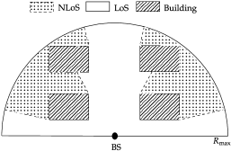
Figure 2: Evaluation scenario: the white area and the dotted areas are in LoS and NLoS conditions, respectively, whereas the UEs are not admitted in the regions occupied by the buildings.

In this section, we present numerical results to validate the proposed algorithms in the three different CSIT configurations, i.e., perfect CSIT (described in Section III), imperfect CSIT (described in Section IV), and topological CSIT (described in Section V). Unless otherwise stated, the considered network topology consists of a semicircular area with radius $R_{\mathrm{\max}}=100$ m where four rectangular buildings are positioned in a Manhattan-like grid, as shown in Fig. 2. We assume that the UEs are distributed uniformly within the network area with the exception of the regions occupied by the buildings and with a minimum distance from the BS of $R_{\mathrm{min}}=5$ m. The direct and D2D links whose line of sight is obstructed by one or more buildings are considered to be in NLoS conditions both in the first and in the second phase. The LoS and NLoS pathloss exponents are fixed to $\alpha=2$ and $\beta=4$, respectively. For simplicity, we assume that all the UEs have the same transmit SNR in the second phase, i.e., $\{\xi_{k}=\xi_{\textnormal{\tiny{UE}}}\}_{k\in\mathcal{K}}$, and we set $\xi_{0}=30$ dB and $\xi_{\textnormal{\tiny{UE}}}=20$ dB. Moreover, unless otherwise stated, the BS is equipped with $M=32$ antennas and the target outage is fixed to $\epsilon=0.1$. Lastly, all the numerical results are averaged over $5\times 10^{3}$ independent UE drops.

VI-A Perfect CSIT

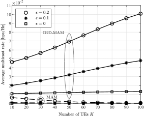
(a) Average multicast rate against the number of UEs with $M=32$ and for different values of $\epsilon$.

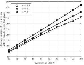
(b) Average number of UEs who are able to decode in the first phase against the number of UEs with $M=32$ and for different values of $\epsilon$.

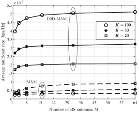
(c) Average multicast rate against the number of BS antennas with $\epsilon=0.1$ and for different values of $K$.

Figure 3: Perfect CSIT: D2D-MAM algorithm versus MAM algorithm.

In the case of perfect CSIT, we evaluate the performance of the proposed D2D-MAM algorithm in Algorithm 1 versus the single-phase MAM algorithm described in Section III-A. Interestingly, the D2D-MAM algorithm converges in very few iterations (typically between $3$ and $10$) even for large values of $K$. Fig. 3(a) plots the average multicast rate against the number of UEs for different values of $\epsilon$. Indeed, the second phase of D2D communications brings substantial gains with respect to traditional multi-antenna multicasting. In particular, the average multicast rate obtained with the D2D-MAM algorithm increases with $K$, whereas that resulting from the MAM algorithm quickly vanishes. Hence, the D2D-MAM algorithm effectively overcomes the worst-UE bottleneck behavior of conventional single-phase multicasting and remarkably achieves an increasing trend of the multicast rate. In the same setting of Fig. 3(a), Fig. 3(b) shows that the average number of UEs who are able to decode in the first phase varies between $35\%$ and $50\%$ of the total UEs depending on the target outage. Lastly, Fig. 3(c) illustrates the average multicast rate against the number of BS antennas for different values of $K$. Evidently, the BS can better focus its transmit power as $M$ increases, which results in an overall improved performance. Here, the lowest value corresponds to $M=1$, i.e., when the BS has no beamforming capability and can only transmit in an isotropic fashion in the first phase.

VI-B Statistical CSIT

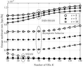
(a) Outage multicast rate against the number of UEs for different values of $c=\frac{K}{M}$.

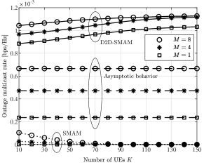
(b) Outage multicast rate against number of UEs for different values $M$.

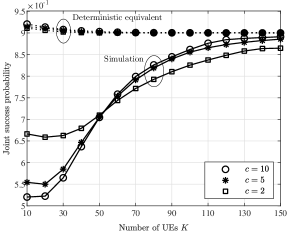
(c) Joint success probability in (11) and its deterministic equivalent in (33) for different values of $c=\frac{K}{M}$.

Figure 4: Statistical CSIT: D2D-SMAM algorithm versus SMAM algorithm.

In the case of statistical CSIT, we evaluate the performance of the proposed D2D-SMAM algorithm in Algorithm 2 versus the single-phase SMAM described in Section IV-A. In addition, we compare the asymptotic expressions obtained in Section IV-C with numerical simulations. For the D2D-SMAM algorithm, we build the set $\mathcal{U}$ by identifying $M$ UEs whose steering angles satisfy the condition in (41), while their distance from the BS is uniformly distributed. We consider two cases of interest, i.e., where both the number of UEs $K$ and the number of BS antennas $M$ increase with a fixed ratio $c=\frac{K}{M}>1$ and where $K$ increases for a fixed $M$. The first case is depicted in Fig. 4(a), which shows that the outage multicast rate always grows as long as $M$ grows together with $K$. The second case is illustrated in Fig. 4(b), which shows how increasing $M$ is always beneficial for any given number of UEs $K$. Here, the outage multicast rate obtained with the D2D-SMAM algorithm grows with $K$ and reaches a constant value for large $K$: this is confirmed by its asymptotic behavior, which is constant with $K$. On the contrary, the SMAM algorithm produces a vanishing outage multicast rate and even increasing $M$ does not fundamentally solve this issue. Lastly, Fig. 4(c) compares the joint success probability in (11) with its deterministic equivalent in (33) for different values of $c$. Here, the approximation is tight for sufficiently large values of $K$.

VI-C Topological CSIT

(a) Evaluation scenario.

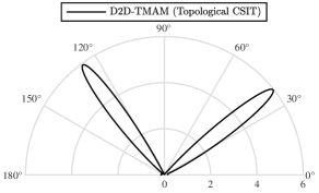
(b) Antenna diagram of the transmit covariance with $M=32$.

Figure 5: Toy example with topological CSIT: the UEs are admitted only in the two white sectors.

In the case of topological CSIT, we evaluate the performance of the proposed D2D-TMAM algorithm in Algorithm 3 versus the D2D-MAM algorithm in Algorithm 1, where the latter is based on the assumption of perfect CSIT. Although unfair to the D2D-TMAM algorithm, this comparison demonstrates how the proposed approach with topological CSIT can accurately sample the long-term network statistics. In turn, this enables to effectively design the precoding strategy at the BS with minimal CSIT requirements and no training overhead without excessively compromising the performance. Let $A$ denote the area of the network excluding the regions occupied by the buildings (expressed in m²) and let us consider a uniform UE distribution with density $\lambda$ (expressed in UEs/m²). In this setting, we assume that each UE drop consists of $K$ UEs, where $K$ is a Poisson random variable with mean $\bar{K}=\lambda A$. Recall that, for the D2D-TMAM algorithm, the transmit covariance and the multicast rate are computed offline by averaging the output of the D2D-MAM algorithm over $L$ batches of $T$ test points, where we fix $L=10^{3}$; on the other hand, the D2D-MAM algorithm is executed for each UE drop.

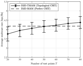
(a) Average multicast rate against number of test points with $M=32$.

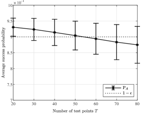
(b) Average success probability against number of test points with $M=32$.

Figure 6: Topological CSIT applied to the toy example in Fig. 5(a): D2D-TMAM algorithm versus D2D-MAM algorithm, where the latter relies on perfect CSIT.

• Toy example. As a first experiment to verify the effectiveness of the proposed method, we consider the simplified network topology depicted in Fig. 5(a), with $R_{\mathrm{max}}=20$ m and where only two sectors admit the presence of UEs. In this setting, we have $A=100$ m² and, fixing $\lambda=0.5$ UEs/m², the average number of UEs in the network is $\bar{K}=50$; moreover, we assume that all the links are in LoS conditions. Fig. 5(b) shows the antenna diagram of the transmit covariance obtained with the D2D-TMAM algorithm with $T=\bar{K}$ test points for each batch: as expected, the multi-antenna beam pattern uniformly covers the two sectors in which the UEs are concentrated. Now, we evaluate the average multicast rate and the average success probability as $T$ varies in order to verify which value gives the best performance. Fig. 6 shows that, when $T$ is too small, the algorithm is overcautious and selects a low multicast rate corresponding to an average success probability above the target; on the other hand, when $T$ is too large, the algorithm is overaggressive and selects a high multicast rate corresponding to an average success probability below the target. As expected, the target outage is reached for $T=\bar{K}$ and the corresponding mean value of the average multicast rate is very close to that obtained with the D2D-MAM algorithm (which relies on perfect CSIT).

Now, let us go back to the original evaluation scenario depicted in Fig. 2 and compare the proposed D2D-TMAM algorithm with the D2D-MAM algorithm. Fig. 7(a) illustrates the average multicast rate against the UE density for different values of $\epsilon$. First of all, we observe that both schemes benefit from increasing the number of UEs, thus effectively overcoming the worst-UE bottleneck behavior of conventional single-phase multicasting. Furthermore, the performance gap between the D2D-TMAM algorithm and the D2D-MAM algorithm is remarkably small despite the huge difference in the CSIT requirements of the two schemes. Lastly, Fig. 7(b) plots the average success probability against the UE density for different values of $\epsilon$, showing that the target success probability is achieved more accurately by the D2D-TMAM algorithm as the UE density increases.

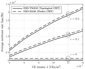
(a) Average multicast rate against UE density with $M=32$ and for different values of $\epsilon$.

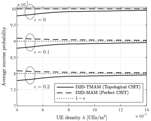
(b) Average success probability against UE density with $M=32$ and for different values of $\epsilon$.

Figure 7: Topological CSIT applied to the evaluation scenario in Fig. 2: D2D-TMAM algorithm versus D2D-MAM algorithm, where the latter relies on perfect CSIT.

VII Conclusion

This paper proposes a general two-phase cooperative multicasting framework that leverages both multi-antenna transmission at the BS and D2D communications between the UEs. We explicitly optimize the precoding strategy at the BS and the multicast rate over the two phases subject to some outage constraint. In particular, we devise efficient algorithms to tackle three different CSIT configurations, i.e., perfect CSIT, statistical CSIT, and topological CSIT. Numerical results show that the proposed schemes significantly outperform conventional single-phase multi-antenna multicasting in all the considered CSIT configurations. Remarkably, they allow to effectively overcome the vanishing behavior of the multicast rate and achieve an increasing performance as the UE population grows large.

Appendix A Proof of Proposition 2

Since problem (40) is convex, a given $\mathbf{\Gamma}_{1}$ is optimal if and only if it satisfies the Karush–Kuhn– Tucker (KKT) conditions. Let us define the Lagrangian and its gradient as

$${\cal L}(\mathbf{\Gamma}_{1},\mu,\mathbf{\Psi}) \triangleq\sum_{k\in\mathcal{K}}\frac{1}{\gamma_{k}\mathbf{a}_{k}^{\mathrm{H}}\mathbf{\Gamma}_{1}\mathbf{a}_{k}}+\mu\big{(}\mathrm{tr}(\mathbf{\Gamma}_{1})-1\big{)}-\mathrm{tr}(\mathbf{\Psi}\mathbf{\Gamma}_{1}),$$ (73)

$$\nabla{\cal L}(\mathbf{\Gamma}_{1},\mu,\mathbf{\Psi}) \triangleq-\sum_{k\in\mathcal{K}}\frac{1}{\gamma_{k}(\mathbf{a}_{k}^{\mathrm{H}}\mathbf{\Gamma}_{1}\mathbf{a}_{k})^{2}}\mathbf{a}_{k}\mathbf{a}_{k}^{\mathrm{H}}+\mu\mathbf{I}_{M}-\mathbf{\Psi}$$ (74)

respectively, where we have introduced the dual variables $\mu\in\mbox{$\mathbb{R}$}$ and $\mathbf{\Psi}\in\mbox{$\mathbb{C}$}^{M\times M}$. The KKT conditions of problem (40) can be written as

$$\sum_{k\in\mathcal{K}}\frac{1}{\gamma_{k}(\mathbf{a}_{k}^{\mathrm{H}}\mathbf{\Gamma}_{1}\mathbf{a}_{k})^{2}}\mathbf{a}_{k}\mathbf{a}_{k}^{\mathrm{H}}=\mu\mathbf{I}_{M}-\mathbf{\Psi},$$ (75a)

$$\mathrm{tr}(\mathbf{\Gamma}_{1})\leq 1,\ \mathbf{\Gamma}_{1}\succeq\mathbf{0},$$ (75b)

$$\mu\geq 0,\ \mathbf{\Psi}\succeq\mathbf{0},$$ (75c)

$$\mu\big{(}\mathrm{tr}(\mathbf{\Gamma}_{1})-1\big{)}=0,\ \mathbf{\Psi}\mathbf{\Gamma}_{1}=\mathbf{0}.$$ (75d)

The condition in (75a) suggests that the transmit covariance has the structure

$$\mathbf{\Gamma}_{1}=\sum_{k\in\mathcal{K}}w_{k}\mathbf{a}_{k}\mathbf{a}_{k}^{\mathrm{H}}$$ (76)

where $\sum_{k\in\mathcal{K}}w_{k}=1/M$ implies $\mathrm{tr}(\mathbf{\Gamma}_{1})=1$ and $\{w_{k}\geq 0\}_{k\in\mathcal{K}}$ implies $\mathbf{\Gamma}_{1}\succeq\mathbf{0}$. From (76), we can write

$$\mathbf{a}_{k}^{\mathrm{H}}\mathbf{\Gamma}_{1}\mathbf{a}_{k} =\sum_{j\in\mathcal{K}}w_{j}\phi_{kj}$$ (77)

where we have defined $\phi_{kj}\triangleq|\mathbf{a}_{k}^{\mathrm{H}}\mathbf{a}_{j}|^{2}$, with $\mathbf{\Phi}\triangleq[\phi_{kj}]_{k,j\in\mathcal{K}}\in\mbox{$\mathbb{C}$}^{K\times K}$ being a symmetric matrix with diagonal elements equal to $M^{2}$. Plugging (76) into (75), the KKT conditions become

$$\sum_{k\in\mathcal{K}}\frac{1}{\gamma_{k}\big{(}\sum_{j\in\mathcal{K}}w_{j}\phi_{kj}\big{)}^{2}}\mathbf{a}_{k}\mathbf{a}_{k}^{\mathrm{H}}=\mu\mathbf{I}_{M}-\mathbf{\Psi},$$ (78a)

$$\sum_{k\in\mathcal{K}}w_{k}=\frac{1}{M},\ \{w_{k}\geq 0\}_{k\in\mathcal{K}},$$ (78b)

$$\mu\geq 0,\ \mathbf{\Psi}\succeq\mathbf{0},$$ (78c)

$$\mu\bigg{(}\sum_{k\in\mathcal{K}}w_{k}-\frac{1}{M}\bigg{)}=0,\ \mathbf{\Psi}\sum_{k}w_{k}\mathbf{a}_{k}\mathbf{a}_{k}^{\mathrm{H}}=\mathbf{0}.$$ (78d)

Let us define $\mathbf{w}\triangleq[w_{1},\ldots,w_{K}]^{\mathrm{T}}\in\mbox{$\mathbb{R}$}^{K\times 1}$. Choosing the weights that satisfy (78b) allows us to set $\mathbf{\Psi}=\mathbf{0}$ and, from (78a), we can show that

$$\mathbf{w}=\frac{1}{\sqrt{\mu M}}\mathbf{\Phi}^{-1}\mathbf{b}$$ (79)

where we have defined

$$\mathbf{b}\triangleq\bigg{[}\frac{1}{\sqrt{\gamma_{1}\mathbf{1}^{\mathrm{T}}\mathbf{\Phi}^{-1}\mathbf{e}_{1}}},\ldots,\frac{1}{\sqrt{\gamma_{K}\mathbf{1}^{\mathrm{T}}\mathbf{\Phi}^{-1}\mathbf{e}_{K}}}\bigg{]}^{\mathrm{T}}.$$ (80)

On the other hand, $\mu$ can be obtained by plugging (79) into the first condition in (78d), i.e.,

$$\mu =M(\mathbf{1}^{\mathrm{T}}\mathbf{\Phi}^{-1}\mathbf{b})^{2}$$ (81)

and, by plugging (81) into (79), we obtain

$$w_{k}=\frac{\mathbf{e}_{k}^{\mathrm{T}}\mathbf{\Phi}^{-1}\mathbf{b}}{M\mathbf{1}^{\mathrm{T}}\mathbf{\Phi}^{-1}\mathbf{b}},\quad\forall k\in\mathcal{K}.$$ (82)

Finally, choosing $\{w_{k}\}_{k\in\mathcal{K}}$ as in (82), $\mu$ as in (81), and $\mathbf{\Psi}=\mathbf{0}$ readily satisfies (78b)–(78d), whereas (78a) yields

$$\sum_{k\in\mathcal{K}}(\mathbf{1}^{\mathrm{T}}\mathbf{\Phi}^{-1}\mathbf{e}_{k})\mathbf{a}_{k}\mathbf{a}_{k}^{\mathrm{H}}=\frac{1}{M}\mathbf{I}_{M}.$$ (83)

The latter is satisfied when $\mathbf{\Phi}=M^{2}\mathbf{I}_{K}$, i.e., when $K=M$ and the steering angles of the UEs are such that $\mathbf{a}_{k}^{\mathrm{H}}\mathbf{a}_{j}=0$, $\forall k\neq j$ (see, e.g., [28] for more details). In this setting, it follows from (82) that $w_{k}=1/(M\sqrt{\gamma_{k}}\nu_{\mathcal{K}})$, from which we obtain the expression of the optimal transmit covariance in (42). ∎

References

- [1] P. Mursia, I. Atzeni, D. Gesbert, and M. Kobayashi, “D2D-aided multi-antenna multicasting,” in Proc. IEEE Int. Conf. Commun. (ICC), Shanghai, China, May 2019.
- [2] P. Mursia, I. Atzeni, M. Kobayashi, and D. Gesbert, “D2D-aided multi-antenna multicasting in a dense network,” in Proc. Asilomar Conf. Signals, Syst., and Comput. (ASILOMAR), Pacific Grove, USA, Nov. 2019.
- [3] N. Jindal and Z.-Q. Luo, “Capacity limits of multiple antenna multicast,” in Proc. IEEE Int. Symp. Inf. Theory (ISIT), Barcelona, Spain, July 2006.
- [4] N. D. Sidiropoulos, T. N. Davidson, and Z.-Q. Luo, “Transmit beamforming for physical-layer multicasting,” IEEE Trans. Signal Process., vol. 54, no. 6, pp. 2239–2251, June 2006.
- [5] A. Khisti, U. Erez, and G. Wornell, “Fundamental limits and scaling behavior of cooperative multicasting in wireless networks,” IEEE Trans. Inf. Theory, vol. 52, no. 6, pp. 2762–2770, June 2006.
- [6] B. Sirkeci-Mergen and M. C. Gastpar, “On the broadcast capacity of wireless networks with cooperative relays,” IEEE Trans. Inf. Theory, vol. 56, no. 8, pp. 3847–3861, July 2010.
- [7] F. Hou, L. X. Cai, P. Ho, X. Shen, and J. Zhang, “A cooperative multicast scheduling scheme for multimedia services in IEEE 802.16 networks,” IEEE Trans. Wireless Commun., vol. 8, no. 3, pp. 1508–1519, Mar. 2009.
- [8] Y. Zhou, H. Liu, Z. Pan, L. Tian, J. Shi, and G. Yang, “Two-stage cooperative multicast transmission with optimized power consumption and guaranteed coverage,” IEEE J. Sel. Areas Commun., vol. 32, no. 2, pp. 274–284, Feb. 2014.
- [9] M. A. Maddah-Ali and U. Niesen, “Fundamental limits of caching,” IEEE Trans. Inf. Theory, vol. 60, no. 5, pp. 2856–2867, May 2014.
- [10] G. Paschos, E. Baştuğ, I. Land, G. Caire, and M. Debbah, “Wireless caching: Technical misconceptions and business barriers,” IEEE Commun. Mag., vol. 54, no. 8, pp. 16–22, Aug. 2016.
- [11] G. Araniti, C. Campolo, M. Condoluci, A. Iera, and A. Molinaro, “LTE for vehicular networking: A survey,” IEEE Commun. Mag., vol. 51, no. 5, pp. 148–157, May 2013.
- [12] V. Ntranos, N. D. Sidiropoulos, and L. Tassiulas, “On multicast beamforming for minimum outage,” IEEE Trans. Wireless Commun., vol. 8, no. 6, pp. 3172–3181, June 2009.
- [13] O. Mehanna, N. D. Sidiropoulos, and G. B. Giannakis, “Joint multicast beamforming and antenna selection,” IEEE Trans. Signal Process., vol. 61, no. 10, pp. 2660–2674, May 2013.
- [14] K.-H. Ngo, S. Yang, and M. Kobayashi, “Scalable content delivery with coded caching in multi-antenna fading channels,” IEEE Trans. Wireless Commun., vol. 17, no. 1, pp. 548–562, Jan. 2018.
- [15] V. Exposito, S. Yang, and N. Gresset, “An information-theoretic analysis of the Gaussian multicast channel with interactive user cooperation,” IEEE Trans. Wireless Commun., vol. 17, no. 2, pp. 899–913, Feb. 2018.
- [16] L. Yang, Q. Ni, L. Lv, J. Chen, X. Xue, H. Zhang, and H. Jiang, “Cooperative non-orthogonal layered multicast multiple access for heterogeneous networks,” IEEE Trans. Commun., vol. 67, no. 2, pp. 1148–1165, Feb. 2019.
- [17] C. Yin, Y. Wang, W. Lin, and J. Xu, “Device-to-device assisted two-stage cooperative multicast with optimal resource utilization,” in Proc. IEEE Global Commun. Conf. (GLOBECOM), Austin, TX, USA, Dec. 2014.
- [18] T. V. Santana, R. Combes, and M. Kobayashi, “Performance analysis of device-to-device aided multicasting in general network topologies,” IEEE Trans. Commun., vol. 68, no. 1, pp. 137–149, Oct. 2020.
- [19] A. Asadi, Q. Wang, and V. Mancuso, “A survey on device-to-device communication in cellular networks,” IEEE Commun. Surveys Tutorials, vol. 16, no. 4, pp. 1801–1819, 4th quarter 2014.
- [20] M. N. Tehrani, M. Uysal, and H. Yanikomeroglu, “Device-to-device communication in 5G cellular networks: Challenges, solutions, and future directions,” IEEE Commun. Mag., vol. 52, no. 5, pp. 86–92, May 2014.
- [21] F. Boccardi, R. W. Heath, A. Lozano, T. L. Marzetta, and P. Popovski, “Five disruptive technology directions for 5G,” IEEE Commun. Mag., vol. 52, no. 2, pp. 74–80, Feb. 2014.
- [22] E. Baştuğ, M. Bennis, and M. Debbah, “Living on the edge: The role of proactive caching in 5G wireless networks,” IEEE Commun. Mag., vol. 52, no. 8, pp. 82–89, Aug. 2014.
- [23] A. Gupta and R. K. Jha, “A survey of 5G network: Architecture and emerging technologies,” IEEE Access, vol. 3, pp. 1206–1232, July 2015.
- [24] Y. Mao, B. Clerckx, J. Zhang, V. O. Li, and M. Arafah, “Max-min fairness of -user cooperative rate-splitting in MISO broadcast channel with user relaying,” IEEE Trans. Wireless Commun., vol. 19, no. 10, pp. 6362–6376, Oct. 2020.
- [25] J. Harri, F. Filali, and C. Bonnet, “Mobility models for vehicular ad hoc networks: A survey and taxonomy,” IEEE Commun. Surveys Tuts., vol. 11, no. 4, pp. 19–41, Dec. 2009.
- [26] A. Destounis, G. S. Paschos, and D. Gesbert, “Selective fair scheduling over fading channels,” in Proc. Int. Symp. Model. and Optim. in Mobile, Ad Hoc and Wireless Netw. (WiOpt), May 2018.
- [27] A. N. Uwaechia and N. M. Mahyuddin, “A comprehensive survey on millimeter wave communications for fifth-generation wireless networks: Feasibility and challenges,” IEEE Access, vol. 8, pp. 62 367–62 414, Mar. 2020.
- [28] A. M. Sayeed, “Deconstructing multiantenna fading channels,” IEEE Trans. Signal Process., vol. 50, no. 10, pp. 2563–2579, Nov. 2002.