Bosonic data hiding: power of linear vs non-linear optics

Abstract

We show that the positivity of the Wigner function of Gaussian states and measurements provides an elegant way to bound the discriminating power of “linear optics”, which we formalise as Gaussian measurement operations augmented by classical (feed-forward) communication (GOCC). This allows us to reproduce and generalise the result of Takeoka and Sasaki [PRA 78:022320, 2008], which tightly characterises the GOCC norm distance of coherent states, separating it from the optimal distinguishability according to Helstrom’s theorem.

Furthermore, invoking ideas from classical and quantum Shannon theory we show that there are states, each a probabilistic mixture of multi-mode coherent states, which are exponentially reliably discriminated in principle, but appear exponentially close judging from the output of GOCC measurements. In analogy to LOCC data hiding, which shows an irreversibility in the preparation and discrimination of states by the restricted class of local operations and classical communication (LOCC), we call the present effect GOCC data hiding.

We also present general bounds in the opposite direction, guaranteeing a minimum of distinguishability under measurements with positive Wigner function, for any bounded-energy states that are Helstrom distinguishable. We conjecture that a similar bound holds for GOCC measurements.

I Introduction

One of the most basic problems of quantum information theory is the discrimination of two alternatives (“hypotheses”), each of which represents the possible state of a system, $\rho_{0}$ or $\rho_{1}$. Under the formalism of quantum mechanics, this calls for the design of a measurement and a decision rule to choose between the two options based on the measurement outcome. The measurement is a binary resolution of unity, also called a positive operator valued measure (POVM), $(M_{0}=M,M_{1}={\openone}-M)$ of two semidefinite operators $M_{0}\,M_{1}\geq 0$ summing to $M_{0}+M_{1}={\openone}$. The outcome $M_{\hat{i}}$ of the measurement is intended to correspond to the estimate $\hat{i}$ of the true state $\rho_{i}$. For simplicity, we will assume that the two hypotheses come with equal (uniform) prior probabilities, so the error probability is

$$\begin{split}P_{e}&=\frac{1}{2}\operatorname{Tr}\rho_{0}({\openone}-M)+\frac{1}{2}\operatorname{Tr}\rho_{1}M\\ &=\frac{1}{2}\bigl{(}1-\operatorname{Tr}(\rho_{0}-\rho_{1})M\bigr{)}.\end{split}$$ (1)

The minimum error over all quantum mechanically allowed POVMs gives rise to the trace norm,

$$\min_{0\leq M\leq{\openone}}P_{e}=\frac{1}{2}\left(1-\frac{1}{2}\|\rho_{0}-\rho_{1}\|_{1}\right),$$ (2)

which formula is nowadays known as Helstrom bound Helstrom ; Helstrom:book or Holevo-Helstrom bound Holevo:dist , since it was initially only proved for projective measurements and subsequently for generalised measurements.

However, from the beginning of quantum detection theory, it was understood that – depending on the physical system – the Helstrom optimal measurement may not be easily implemented. Indeed, the very example of discrimination of to coherent states of an optical mode was already considered by Helstrom Helstrom:coherent , who contrasted the absolutely minimum error probability with the performance of reasonable practical measurements. Mathematically, this means that the minimisation on the l.h.s. of Eq. (2) is performed over a smaller set of POVMs, the restriction an expression of what is deemed physically feasible. Consequently, the error probability becomes larger, in some interesting cases close to $\frac{1}{2}$ even for orthogonal, i.e. ideally perfectly distinguishable, states. This phenomenon was first observed in bipartite systems under the restriction of local operations and classical communication (LOCC), and dubbed data hiding Terhal-datahiding ; DiVincenzo-datahiding , which has been generalised to multi-party settings EggelingWerner , and analysed extensively MWW ; LW ; W:eff .

In the present paper we will look at a different kind of restriction, in Bosonic quantum systems, motivated by the distinction between phase-space linear (aka Gaussian) and non-linear (i.e. non-Gaussian) operations, see also KKVV . It is well-known that a process that starts from a Gaussian state and proceeds only via Gaussian operations, including Gaussian measurements and classical feed-forward (GOCC, see below), is in a certain sense very far away from the full complexity of quantum mechanics: indeed, such a process can be simulated efficiently on a classical computer bartlett ; mari and hence, unless BQP=BPP, is not quantum computationally universal. In other words, non-Gaussianity is a resource for computation, which it becomes quite explicitly in proposals of optical quantum computing such as the Knill-Laflamme-Milburn scheme KLM that relies on photon detection and otherwise passive linear optics.

Here we show that non-Gaussianity is a resource for the basic task of binary hypothesis testing. In particular we show how to leverage simple properties of the Wigner function to prove not only a limitation of the power of Gaussian operations, but construct data hiding with respect to GOCC.

To conclude the introduction, a word on terminology: we refer to Gaussian states and channels as “linear”, because the latter are described by linear transformations in the phase space of the canonical variables $x$ and $p$. Conversely, “non-linear” is anything outside the Gaussian set. Note however that in parts of quantum optics a narrower concept is used, whereby only channels are considered linear that are built with passive Gaussian unitaries, and perhaps admitting displacement operators.

The rest of paper is structured as follows: In the next section (II) we recall the necessary formalism and notation of quantum harmonic oscillators and Gaussian Bosonic states and operations; for our purposes in particular useful will be the phase space methods based on Wigner functions. Then, in Section III we specialise the general framework of restricted measurements to Gaussian quantum operations and arbitrary classical computations (GOCC), and the important relaxation of this class to measurements with non-negative Wigner functions (W+). We use these in Section IV to analyze the optimal GOCC measurement to distinguish two coherent states, reproducing (with a conceptually much simpler proof) a result of Takeoka and Sasaki TakeokaSasaki . The GOCC distinguishability of any two distinct coherent states is always a little, but always strictly worse than the optimal distingishability according to Helstrom Helstrom ; Holevo:dist . Motivate by this, in Section V we exhibit examples of multimode states, each a mixture of coherent states (hence “classical” in the quantum-optical sense Glauber ; Sudarshan and in particular preparable by GOCC), whose GOCC distinguishability is exponentially small while they are almost perfectly distinguishable under the optimal Holevo-Helstrom measurement. From the other side, there are lower limits to how indistinguishable two orthogonal states on $n$ quantum harmonic modes and with bounded energy can be, which we show for W+ measurements and conjecture for GOCC measurements (Section VI). We conclude in Section VII.

II Bosonic Gaussian formalism

We briefly review the formalism of Bosonic systems and Gaussian states, which has been laid out in many review articles and textbooks, such as Weedbrook-et-al and Barnett ; KokLovett , which two emphasise the quantum information aspect. For our particular choice of normalisations, see cahill .

Each elementary system, called a (harmonic) mode, is characterised by a pair of canonical variables $x$ and $p$, satisfying the canonical commutation relation (CCR) $[x,p]=i$ (customarily choosing units where $\hbar=1$) and generating the CCR algebra of Heisenberg and Weyl. By the Stone-von-Neumann theorem, each irreducible representation of this algebra on a separable Hilbert space $\mathcal{H}$ is isomorphic to the usual position and momentum operators $x$ and $p$, respectively.

It is convenient to introduce the annihilation and creation operators

$$a=\frac{x+ip}{\sqrt{2}},\quad a^{\dagger}=\frac{x-ip}{\sqrt{2}},$$ (3)

respectively. They can be used to define the number operator,

$$N=a^{\dagger}a=\frac{1}{2}(x^{2}+p^{2})-\frac{1}{2}=\sum_{n=0}^{\infty}n\,|n\rangle\!\langle n|,$$ (4)

which up to the energy shift of $-\frac{1}{2}$ to bring the ground state energy to zero, is equivalent to the quantum harmonic Hamiltonian (at fixed frequency), and has precisely the non-negative integers as eigenvalues; the eigenstates are known as Fock states or number states, $|n\rangle$. In the number basis,

$$a=\sum_{n=0}^{\infty}\sqrt{n}\,|n\!-\!1\rangle\!\langle n|,\quad a^{\dagger}=\sum_{n=0}^{\infty}\sqrt{n}\,|n\rangle\!\langle n\!-\!1|.$$ (5)

All these operators are unbounded, and one might have justified hesitations against the algebraic operations performed above. The established solution to all of the potential problems associated to the unboundedness and associated restricted domains is to pass to the displacement operators,

$$D(\alpha)=e^{\alpha a^{\dagger}-\overline{\alpha}a},\text{ for }\alpha\in{{\mathbb{C}}},$$ (6)

which are bona fide unitaries, hence bounded operators.

So far, we have discussed our quantum system at hand as if it were a single mode, but we can of course consider multi-mode systems, which again by the Stone-von-Neumann theorem are characterised uniquely as irreducible representations of the CCR algebra generated by $x_{1},\ldots,x_{m}$ and $p_{1},\ldots,p_{m}$ such that $[x_{j},p_{k}]=i\delta_{jk}$. This means that its Hilbert space can be identified with $\mathcal{H}_{1}\otimes\cdots\otimes\mathcal{H}_{m}$, where $\mathcal{H}_{j}$ is the Hilbert space of the $j$-th mode, carrying the representation of $x_{j}$ and $p_{j}$. In particular, each mode has its own annihilation operator $a_{j}$ and displacement operator $D(\alpha)$; for an $m$-tuple $\underline{\alpha}=(\alpha_{1},\ldots,\alpha_{m})$ of displacements, we write $D(\underline{\alpha})=D(\alpha_{1})\otimes\cdots\otimes D(\alpha_{m})$ for the $m$-mode displacement operator. The subspace spanned by these operators is dense in the bounded operators $\mathcal{B}(\mathcal{H})$ on the Hilbert space.

For a general density operator $\rho\in\mathcal{S}(\mathcal{H})=\{\rho\geq 0,\ \operatorname{Tr}\rho=1\}$, or more generally for a trace class operator, the characteristic function is defined as

$$\chi_{\rho}(\underline{\alpha})\mathrel{\mathop{\mathchar 58\relax}}=\operatorname{Tr}\rho D(\underline{\alpha}).$$ (7)

This is a bounded complex function, uniquely specifying $\rho$. A state $\rho$ is called Gaussian if its characteristic function $\chi_{\rho}$ is of Gaussian form. For our purposes, we need another, particularly useful representation of the state as a quasi-probability function, the so-called Wigner function $W_{\rho}$ Wigner ; HOCSW , see also Barnett ; cahill for many fundamental and useful relations such as the following two. It is defined as the (multidimensional complex) Fourier transform of the characteristic function $\chi_{\rho}$,

$$W_{\rho}(x,p)=\left(\frac{1}{2\pi^{2}}\right)^{m}\int{\rm d}^{2m}\underline{\xi}\,e^{\underline{\alpha}\cdot\underline{\xi}^{\dagger}-\underline{\xi}\cdot\underline{\alpha}^{\dagger}}\chi_{\rho}(\underline{\xi}),$$ (8)

where we reparametrise the argument in phase space coordinates, $\alpha_{j}=\frac{1}{\sqrt{2}}(x_{j}+ip_{j})$, and $\underline{\alpha}\cdot\underline{\xi}^{\dagger}=\sum_{j}\alpha_{j}\overline{\xi}_{j}$ is the Hermitian inner product of the complex coordinate tuples. This is a real-valued function, and its normalisation is chosen in such a way that

$$\int{\rm d}^{m}x{\rm d}^{m}p\,W_{\rho}(x,p)=\operatorname{Tr}\rho,$$ (9)

hence for a state we can address it as a quasi-probability function as it integrates to $1$, and if the Wigner function is positive it is a genuine probability density. In general, can be expressed as an expectation value, cf. Barnett ; cahill ,

$$W_{\rho}(x,p)=\pi^{-m}\operatorname{Tr}\rho D(\underline{\alpha})(-1)^{N_{1}+\ldots+N_{m}}D(\underline{\alpha})^{\dagger}.$$ (10)

where as before $\alpha_{j}=\frac{1}{\sqrt{2}}(x_{j}+ip_{j})$. It shows that $W_{\rho}$ is well-defined and indeed a continuous bounded function for all trace class operators: indeed, $|W_{\rho}(x,p)|\leq\pi^{-m}\|\rho\|_{1}$. The above formula can be used to give meaning to more general operators (such as POVM elements); for instance the Wigner function of the identity operator is a constant, $W_{\openone}=(2\pi)^{-m}$. The Wigner transformation preserves the Frobenius (Hilbert-Schmidt) inner product,

$$\operatorname{Tr}\rho\sigma=(2\pi)^{m}\int{\rm d}^{m}x{\rm d}^{m}p\,W_{\rho}(x,p)W_{\sigma}(x,p).$$ (11)

Unitary transformations of the Hilbert space preserve the canonical commutation relations; but the subset of unitaries that map the Lie algebra of the canonical variables, which is $\operatorname{span}\{{\openone},x_{j},p_{k}\}$, to itself, are called Gaussian unitaries. We address them also as “linear” transformations, since they are correspond to an affine linear map of phase space, and are described by a displacement vector and a symplectic matrix. Gaussian channels are precisely the completely positive and trace preserving (cptp) maps taking Gaussian states to Gaussian states. It is a fundamental fact that a quantum channel $\mathcal{N}\mathrel{\mathop{\mathchar 58\relax}}\mathcal{S}(\mathcal{H})\rightarrow\mathcal{S}(\mathcal{H}^{\prime})$ is Gaussian if and only if it has a Gaussian unitary dilation $U$, with the environment initialised in the vacuum state:

$$\mathcal{N}(\rho)=\operatorname{Tr}_{E}U\left(\rho\otimes|0\rangle\!\langle 0|^{\otimes\ell}\right)U^{\dagger},$$ (12)

where the environment has $\ell$ modes.

For the following, we need the (Glauber-Sudarshan) coherent states, also known as minimal dispersion states $|\alpha\rangle$, which are eigenstates of the annihilation operator: $a|\alpha\rangle=\alpha\,|\alpha\rangle$, for $\alpha\in{{\mathbb{C}}}$. This defines the states uniquely, and one can show that they are related by displacements: $|\alpha\rangle=D(\alpha)|0\rangle$, where $|0\rangle$ is both the coherent state corresponding to $\alpha=0$ and the vacuum, i.e. the ground state of the Hamiltonian, in other words the zeroth Fock state. In the Fock basis,

$$|\alpha\rangle=e^{-\frac{1}{2}|\alpha|^{2}}\sum_{n=0}^{\infty}\frac{\alpha^{n}}{\sqrt{n!}}|n\rangle,$$ (13)

a relation that reassuringly shows that the coherent states are well-defined unit vectors, written in a genuine orthonormal basis. However, what is more relevant are the following expressions for the first and second moments. For $\alpha=\alpha_{R}+i\alpha_{I}$ written in terms of real and imaginary parts,

$$\langle\alpha|x|\alpha\rangle =\alpha_{R}\sqrt{2},\ \langle\alpha|p|\alpha\rangle=\alpha_{I}\sqrt{2},$$ (14)

$$\langle 0|x^{2}|0\rangle =\langle 0|p^{2}|0\rangle=\frac{1}{2},$$ (15)

the latter “vacuum fluctuations” consistent with the Heisenberg-Robertson uncertainty relation. Furthermore, the inner product, easily confirmed from the expansion in the Fock basis,

$$|\langle\alpha|\beta\rangle|^{2}=e^{-|\alpha-\beta|^{2}}.$$ (16)

And finally, we record

$$\frac{1}{\pi}\int{\rm d}\alpha\,|\alpha\rangle\!\langle\alpha|={\openone},$$ (17)

showing that the family of operators $\frac{{\rm d}\alpha}{\pi}|\alpha\rangle\!\langle\alpha|$ forms a POVM, known as heterodyne measurement.

III State discrimination by
Gaussian measurements

Now that we have the Bosonic formalism in place, we can discuss the problem of binary hypothesis testing under Gaussian restrictions on the measurement. Indeed, going back to Eqs. (1) and (2) in the introduction, almost any restriction $\mathbb{M}$ on the set of possible measurements, be they physically motivated or purely mathematical, results in a larger error probability than the Helstrom expression, which is most conveniently expressed in terms of a distinguishability norm on states:

$$\min_{(M,{\openone}-M)\in\mathbb{M}}P_{e}=\mathrel{\mathop{\mathchar 58\relax}}\frac{1}{2}\left(1-\frac{1}{2}\|\rho_{0}-\rho_{1}\|_{\mathbb{M}}\right).$$ (18)

How to define the set $\mathbb{M}$ appropriately and what exactly is necessary for it to define a norm is explained in detail in MWW . An example exceedingly well-studied in quantum information theory is the set of measurements implemented by local operations and classical communication (LOCC) in a bi- or multi-partite system, as well as its relaxations separable POVM elements (SEP) and POVM elements with positive partial transpose (PPT), cf. MWW ; LOCC:always

Here, we consider restrictions motivated from the fact that Gaussian operations are distinguished among the ones allowed by quantum mechanics generally, following Takeoka and Sasaki TakeokaSasaki . Concretely, we are interested in the measurements implemented by any sequence of partial Gaussian POVMs and classical feed-forward (Gaussian operations and classical computation, GOCC). Very much like LOCC, there is no concise way of writing down a general GOCC transformation, but for a binary measurement the prescription is as follows.

Definition 1

A GOCC measurement protocol on $m$ modes consists of the repetition of the following steps, for $r=1,\ldots,R$ (“rounds”), after initially setting $\xi_{0}=\emptyset$ and $m_{\emptyset}=m$. Here, $\xi_{r-1}$ is the collection of all measurement outcomes prior to round $r$.

• create a number $k_{\xi_{r-1}}$ of Bosonic modes in the vacuum state;

• perform a Gaussian unitary $U_{\xi_{r-1}}$ on the $m_{\xi_{r-1}}+k_{\xi_{r-1}}$ modes;

• perform homodyne detection on the last $\ell_{\xi_{r-1}}$ modes, keeping the first $m_{\xi_{r}}\mathrel{\mathop{\mathchar 58\relax}}=m_{\xi_{r-1}}+k_{\xi_{r-1}}-\ell_{\xi_{r-1}}$; call the outcome $\underline{x}^{(r)}=x_{1}^{(r)}\ldots x_{\ell_{\xi_{r-1}}}^{(r)}$ and set $\xi_{r}\mathrel{\mathop{\mathchar 58\relax}}=\{\xi_{r-1},\underline{x}^{(r)}\}$.

Each $r$ is called a “round”, and in the $R$-th round all remaining modes are measured, i.e. $\ell_{\xi_{r-1}}=m_{\xi_{r-1}}+k_{\xi_{r-1}}$. The final measurement outcome is a measurable function $f(\xi_{R})\in\Omega$, taking values in a prescribed set $\Omega$, which for simplicity we assume to be discrete.

This defines a POVM $(M_{\omega}\mathrel{\mathop{\mathchar 58\relax}}\omega\in\Omega)$, and every POVM that arises in the above way, or as a limit of such POVMs in the strong topology is called a GOCC POVM.

Now, returning to equiprobable hypotheses $\rho_{0}$ and $\rho_{1}$, and enforcing the POVMs to be implemented by GOCC protocols, we arrive at the GOCC norm:

$$\inf_{(M,{\openone}-M)\atop\text{GOCC POVM}}P_{e}=\mathrel{\mathop{\mathchar 58\relax}}\frac{1}{2}\left(1-\frac{1}{2}\|\rho_{0}-\rho_{1}\|_{\mathrm{GOCC}}\right).$$ (19)

Note that $\|\cdot\|_{\mathrm{GOCC}}$ is indeed a norm, since the set of GOCC measurements is tomographically complete. Indeed, heterodyne detection on every available mode is a tomographically complete measurement, meaning that for every pair of distinct quantum states, there exists a binary coarse graining of the heterodyne detection outcomes that discriminates the states with some non-zero bias.

Remark 2

In the definition of a GOCC protocol, we could have allowed the $k_{\xi_{r-1}}$ ancillary modes to be prepared in any Gaussian state in step (r.1), but that does not add any more generality, since every Gaussian state can be prepared from the vacuum by a suitable Gaussian unitary. We could also have allowed an arbitrary Gaussian quantum channel in step (r.2), but again that does not add any more generality since every Gaussian channel has a dilation to a Gaussian unitary with an environment prepared in the vacuum state. Finally, in step (r.3) we could have allowed any Gaussian measurement, but every Gaussian measurement can be implemented by adjoining suitable ancilla modes in the vacuum, performing a Gaussian unitary and a homodyne measurement.

From the point of view of the discussion of classes of operations, of which measurements are a special case, it is interesting to distinguish certain subclasses of GOCC: what we actually have defined are the measurements implemented by a GOCC protocol with finitely many rounds, as well as the closure of this set. One could also define the POVMs implemented by a GOCC protocol with unbounded rounds (but probability 1 to stop), which would sit between the former two, cf. LOCC:always for the case of LOCC. While it is interesting to study these three classes, in particular whether they coincide or are separated (as they are in the analogous case of LOCC LOCC:always ) this is beyond the scope of the present work. Indeed, for the case of hypothesis testing, thanks to the infimum in the error probability, all three classes will give rise to the same GOCC norm.

An elementary observation about GOCC is that the fine-grained measurement (i.e. before coarse-graining to a discrete POVM) consists of operators each of which is a positive scalar multiple of a Gaussian pure state. In particular, they have non-negative Wigner function, and because the coarse-graining amounts to summing POVM elements, also the final POVM has non-negative Wigner functions. We thus call a binary POVM $(M,{\openone}-M)$ with non-negative Wigner functions $W_{M}$ and $W_{{\openone}-M}$ a W+ POVM, and denote their set $\mathbb{W}_{+}$.

Just as the restriction to GOCC leads to the distinguishability norm $\|\cdot\|_{\mathrm{GOCC}}$ [Eq. (19)], the restriction to W+ POVMs gives rise to the distinguishability norm $\|\cdot\|_{\mathrm{W+}}$:

$$\inf_{(M,{\openone}-M)\atop\text{W+ POVM}}P_{e}=\mathrel{\mathop{\mathchar 58\relax}}\frac{1}{2}\left(1-\frac{1}{2}\|\rho_{0}-\rho_{1}\|_{\mathrm{W+}}\right).$$ (20)

Since every GOCC measurement is automatically W+, we have by definition

$$\|\rho_{0}-\rho_{1}\|_{\mathrm{GOCC}}\leq\|\rho_{0}-\rho_{1}\|_{\mathrm{W+}}\leq\|\rho_{0}-\rho_{1}\|_{1}.$$ (21)

The rest of the paper is concerned with the comparison of these norms. The questions guiding us are: are they different, and how large are the gaps?

IV Separation between GOCC and unrestricted measurements

Our first result shows a simple upper bound on the GOCC and W+ distinguishability norms in terms of the Wigner functions of the two states.

Lemma 3

For any two states $\rho_{0}$ and $\rho_{1}$ of an $m$-mode system, with associated Wigner functions $W_{0}$ and $W_{1}$, respectively,

$$\begin{split}\|\rho_{0}-\rho_{1}\|_{\mathrm{GOCC}}&\leq\|\rho_{0}-\rho_{1}\|_{\mathrm{W+}}\\ &\leq\|W_{0}-W_{1}\|_{L^{1}}\\ &=\int{\rm d}^{m}x{\rm d}^{m}p\,|W_{0}(x,p)-W_{1}(x,p)|.\end{split}$$

Note that, unlike the inequalities (21), the third term in the chain is not a trace norm of density matrices, but an $L^{1}$ norm of real functions, which we may interpret as generalised densities.

Proof.

Only the second inequality remains to be proved. Consider any W+ POVM $(M,{\openone}-M)$, meaning that the stochastic response functions $F=(2\pi)^{m}W_{M}$ and $1-F=(2\pi)^{m}W_{{\openone}-M}$ are bounded between $0$ and $1$. By the Frobenius inner product formula for the Wigner function, Eq. (11), we have

$$\operatorname{Tr}(\rho_{0}-\rho_{1})M=\int{\rm d}^{m}x{\rm d}^{m}p\,\bigl{(}W_{0}(x,p)-W_{1}(x,p)\bigr{)}F(x,p),$$ (22)

where the left hand side appears in Eq. (1), its supremum over W+ POVMs being $\frac{1}{2}\|\rho_{0}-\rho_{1}\|_{\mathrm{W+}}$; while the right hand side is upper bounded by $\frac{1}{2}\|W_{0}-W_{1}\|_{L^{1}}$, where we made use of the fact that $\int{\rm d}^{m}x{\rm d}^{m}p\,(W_{0}(x,p)-W_{1}(x,p))=\operatorname{Tr}(\rho_{0}-\rho_{1})=0$. ∎

Remark 4

The lemma assumes measurements with W+ POVMs, but it gives interesting information also in cases where the POVM has some limited Wigner negativity. Namely, looking at Eq. (22), we subsequently use that $0\leq F(x,p)\leq 1$, which is the property W‘+ of the measurement.

If we do not have “too much” Wigner negativity in the measurement operators, this could be expressed by a bound $|2F(x,p)-1|\leq B$, and then we would get

$$\bigl{|}\operatorname{Tr}(\rho_{0}-\rho_{1})M\bigr{|}\leq\frac{B}{2}\|W_{0}-W_{1}\|_{L^{1}}.$$ (23)

The right hand side can still be small when the $L^{1}$-distance is really small, and at the same time $B$ not too large. In the next section we shall see an example of this.

As one might expect, the inequality in Lemma 3 is often crude, or even trivial since one can find states where the right had side exceeds $2$. However, if $\rho_{0}$ and $\rho_{1}$ are both states with non-negative Wigner function, for instance probabilistic mixtures of Gaussian states, then $W_{0}$ and $W_{1}$ are bona fide probability densities, and the right hand side is $\leq 2$. In that case, we have the following corollary for the quantum Chernoff coefficient when measurements are restricted to GOCC or W+ POVMs. Recall that the Chernoff coefficient is the exponential rate of the minimum error probability in distinguishing two i.i.d. hypotheses. I.e., in the case of two quantum states

$$\xi(\rho_{0},\rho_{1})\mathrel{\mathop{\mathchar 58\relax}}=\lim_{n\rightarrow\infty}-\frac{1}{n}\ln\left(1-\frac{1}{2}\left\|\rho_{0}^{\otimes n}-\rho_{1}^{\otimes n}\right\|_{1}\right),$$ (24)

which generalises the analogous question for probability distributions Chernoff . Amazingly, there is a formula for this exponent q-Chernoff , generalising in its turn the classical answer Chernoff :

$$\xi(\rho_{0},\rho_{1})=-\ln\inf_{0<s<1}\operatorname{Tr}\rho_{0}^{s}\rho_{1}^{1-s}.$$ (25)

Just as the distinguishability norm under a restriction, we can then define the constrained Chernoff coefficient, if the restriction $\mathbb{M}$ describes a subset of POVMs for each number of elementary systems:

$$\xi_{\mathbb{M}}(\rho_{0},\rho_{1})\mathrel{\mathop{\mathchar 58\relax}}=\lim_{n\rightarrow\infty}-\frac{1}{n}\ln\left(1-\frac{1}{2}\left\|\rho_{0}^{\otimes n}-\rho_{1}^{\otimes n}\right\|_{\mathbb{M}}\right).$$ (26)

Corollary 5

For two states $\rho_{0}$ and $\rho_{1}$ with non-negative Wigner functions $W_{0},\,W_{1}\geq 0$ (meaning that they are probability density functions),

$$\xi_{\mathrm{GOCC}}(\rho_{0},\rho_{1})\leq\xi_{\mathrm{W+}}(\rho_{0},\rho_{1})\leq\xi(W_{0},W_{1}),$$

where according to Chernoff’s theorem Chernoff ,

$$\xi(W_{0},W_{1})=-\ln\inf_{0<s<1}\int{\rm d}^{m}x{\rm d}^{m}p\,W_{0}(x,p)^{s}W_{1}(x,p)^{1-s}$$

is the classical Chernoff coefficient of the probability distributions $W_{0}$ and $W_{1}$. ∎

As in Lemma 3, the third term in the chain is not a quantity of density matrices, but of classical probability densities.

It is not difficult to find examples where the bounds of the Lemma and its Corollary are exactly tight, among them the case of two coherent states studied originally by Takeoka and Sasaki TakeokaSasaki .

Example 6

Consider $\rho_{0}$ and $\rho_{1}$ as two coherent states of a single mode, say $\rho_{0}=|+\alpha\rangle\!\langle+\alpha|$, $\rho_{1}=|-\alpha\rangle\!\langle-\alpha|$ for $\alpha>0$. Then,

$$\frac{1}{2}\|\rho_{0}-\rho_{1}\|_{1}=\sqrt{1-e^{-4\alpha^{2}}}.$$ (27)

while by Lemma 3,

$$\frac{1}{2}\|\rho_{0}-\rho_{1}\|_{\mathrm{GOCC}}=\frac{1}{2}\|\rho_{0}-\rho_{1}\|_{\mathrm{W+}}=\operatorname{erf}(\alpha\sqrt{2}),$$ (28)

with the error function $\operatorname{erf}(x)=\frac{2}{\sqrt{\pi}}\int_{0}^{x}{\rm d}x\,e^{-x^{2}}$. The equality follows from homodyning the $x$-coordinate and deciding depending on the sign of the measurement outcome. The norms are compared in Fig. 1.

Furthermore, in the asymptotic i.i.d. setting of the Chernoff bound,

$$\xi(\rho_{0},\rho_{1})=-\ln F(\rho_{0},\rho_{1})^{2}=4|\alpha|^{2},$$ (29)

while by Corollary 5,

$$\xi_{\mathrm{GOCC}}(\rho_{0},\rho_{1})=\xi_{\mathrm{W+}}(\rho_{0},\rho_{1})=2|\alpha|^{2}.$$ (30)

The equality follows from homodyning each mode separately in the $x$ direction, and classical post-processing.

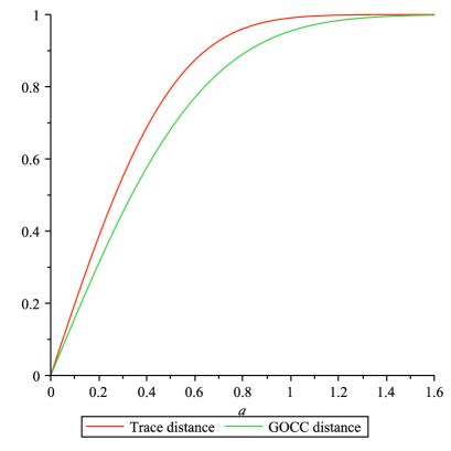
Figure 1: Plot of the trace distance (red) versus the GOCC distance (green) against $\alpha$ on the horizontal axis. While there is a nonzero gap for all $\alpha>0$, it vanishes for asymptotically large and small displacements, as expected. The largest difference between $\frac{1}{2}\|\rho_{0}-\rho_{1}\|_{1}$ and $\frac{1}{2}\|\rho_{0}-\rho_{1}\|_{\mathrm{GOCC}}$ is $\approx 0.11$, occurring at $\alpha\approx 0.45$.

Example 7

More generally, for any one-mode Gaussian state and its displacement along one of the principal axes of the covariance matrix,

$$\|\rho_{0}-\rho_{1}\|_{\mathrm{GOCC}}=\|\rho_{0}-\rho_{1}\|_{\mathrm{W+}}=\|W_{0}-W_{1}\|_{L^{1}},$$ (31)

and the latter can be expressed in terms of the error function and the shared variance of the two states in the direction of the displacement connecting them.

The equality follows from homodyning in the direction of the line connecting the two first moment vectors in phase space, and deciding depending on which of the two points is closer to the outcome.

V Data hiding secure against Gaussian attacker

As soon as we realize that it is possible to get large gaps between $\|\cdot\|_{1}$ and $\|\cdot\|_{\mathrm{GOCC}}$, we have to ask ourselves, just how large the gap can be. In particular, is it possible to find state pairs which are almost maximally distant in the trace norm, yet almost indistinguishable in the GOCC norm? In other words, can we protect the information against an adversary who attempts the hypothesis testing on the two states but with only access to Gaussian operations and classical communication? This is the definition of data hiding, first explored in the context of the LOCC restriction, and then later abstractly for an arbitrary restriction on the possible measurements.

Next we shall show that data hiding is possible also under GOCC, at least when going to multiple modes.

Theorem 8

Let $\overline{E}>0$. Then, there is a constant $c>0$ such that for all sufficiently large integers $m$ there exist $m$-mode states $\rho_{0}$ and $\rho_{1}$, each a mixture of a finite set of coherent states and with average energy (photon number) per mode bounded by $\overline{E}+o(1)$, such that

$$\frac{1}{2}\|\rho_{0}\!-\!\rho_{1}\|_{1} \geq 1-e^{-cm},$$ (32)

$$e^{-cm} \geq\frac{1}{2}\|\rho_{0}\!-\!\rho_{1}\|_{\mathrm{W+}}\geq\frac{1}{2}\|\rho_{0}\!-\!\rho_{1}\|_{\mathrm{GOCC}}.$$ (33)

Proof.

Consider the $m$-mode coherent states $|\underline{\alpha}^{(\lambda)}\rangle=|\alpha^{(\lambda)}_{1}\rangle|\alpha^{(\lambda)}_{2}\rangle\cdots|\alpha^{(\lambda)}_{m}\rangle$ ($\lambda=1,\ldots,2L$), where the parameters $\alpha^{(\lambda)}_{j}\in{{\mathbb{C}}}$ are chosen i.i.d according to a normal distribution with mean $0$ and variance ${{\mathbb{E}}}|\alpha^{(\lambda)}_{j}|^{2}=\overline{E}$. Then define

$$\begin{split}\rho_{0}&=\frac{1}{L}\sum_{\lambda=1}^{L}|\underline{\alpha}^{(2\lambda)}\rangle\!\langle\underline{\alpha}^{(2\lambda)}|,\\ \rho_{1}&=\frac{1}{L}\sum_{\lambda=1}^{L}|\underline{\alpha}^{(2\lambda-1)}\rangle\!\langle\underline{\alpha}^{(2\lambda-1)}|,\end{split}$$ (34)

so these are random states. Note that with high probability, indeed asymptotically converging to $1$ as $m\gg 1$, both have their photon number per mode bounded by $\overline{E}+o(1)$. Also,

$${{\mathbb{E}}}\rho_{0}={{\mathbb{E}}}\rho_{1}=\gamma(\overline{E})^{\otimes m},$$ (35)

where $\gamma(\overline{E})=(1-e^{-\beta})e^{-\beta N}$ is the thermal state of a single Bosonic mode of mean photon number $\overline{E}$, i.e. with $\beta=\ln\left(1+\frac{1}{\overline{E}}\right)$.

The rest of the proof will consist in showing that we can fix $L$ in such a way that with probability close to $1$, $\rho_{0}$ and $\rho_{1}$ are distinguishable except with exponentially small error probability, and that with probability close to $1$, the Wigner functions $W_{0}$ and $W_{1}$ are exponentially close to $W_{\gamma(\overline{E})}^{\otimes m}$, the Wigner function of $\gamma(\overline{E})^{\otimes m}$, in the total variational distance.

Eq. (32): The ensemble of coherent states $|\underline{\alpha}^{(\lambda)}\rangle$ is the well-studied random coherent state modulation of the noiseless Bosonic channel with input power (photon number) $\overline{E}$, whose classical capacity is well-known pure-loss-C , with the strong converse proved in WiWi:pure-loss .

$$\begin{split}C({\operatorname{id}},\overline{E})&=g(\overline{E})\\ &=(\overline{E}+1)\ln(\overline{E}+1)-\overline{E}\ln\overline{E}\\ &=\ln(1+\overline{E})+\overline{E}\ln\left(1+\frac{1}{\overline{E}}\right).\end{split}$$ (36)

Thus, when $2L\leq e^{m\bigl{(}C({\operatorname{id}},\overline{E})-\delta\bigr{)}}$, it follows from the Holevo-Schumacher-Westmoreland theorem Holevo:C ; SchumacherWestmoreland:C ; Holevo:C-E that with probability close to $1$, there exists a POVM $(D_{\lambda})_{\lambda=1}^{2L}$ that decodes $\lambda$ reliably from the state $|\underline{\alpha}^{(\lambda)}\rangle\!\langle\underline{\alpha}^{(\lambda)}|$:

$$\frac{1}{2L}\sum_{\lambda=1}^{2L}\operatorname{Tr}|\underline{\alpha}^{(\lambda)}\rangle\!\langle\underline{\alpha}^{(\lambda)}|D_{\lambda}\geq 1-e^{-c^{\prime}m},$$ (37)

with a suitable constant $c^{\prime}>0$ and for all sufficiently large $m$. Thus, with $\rho_{i}$ ($i=0,1$) as defined above and

$$M_{i}=\sum_{\lambda=1}^{L}D_{2\lambda-i}\quad(i=0,1),$$ (38)

it follows

$$\frac{1}{2}\operatorname{Tr}\rho_{0}M_{0}+\frac{1}{2}\operatorname{Tr}\rho_{1}M_{1}\geq 1-e^{-c^{\prime}m},$$ (39)

which implies Eq. (32).

Eq. (33): The Wigner functions $W_{\underline{\alpha}^{(\lambda)}}$ of the coherent states $|\underline{\alpha}^{(\lambda)}\rangle\!\langle\underline{\alpha}^{(\lambda)}|$ are $2m$-dimensional real Gaussian probability densities centered at $\underline{z}^{(\lambda)}$, where $z^{(\lambda)}_{2j-1}=\Re\alpha^{(\lambda)}_{j}\sqrt{2}$ and $z^{(\lambda)}_{2j}=\Im\alpha^{(\lambda)}_{j}\sqrt{2}$ are the rescaled real and imaginary part of $\underline{\alpha}^{(\lambda)}_{j}$, respectively; they have variance $\frac{1}{2}$ in each direction. We read them as output distributions of an i.i.d. additive white Gaussian noise (AWGN) channel on $2m$ inputs $\underline{z}^{(\lambda)}$, and with noise power $\frac{1}{2}$. Note that all $z^{(\lambda)}_{j}$ are themselves Gaussian distributed random variables with ${{\mathbb{E}}}z^{(\lambda)}_{j}=0$ and ${{\mathbb{E}}}|z^{(\lambda)}_{j}|^{2}=\overline{E}$. This channel, which we denote $\widetilde{W}$ since its output distributions come from the Wigner functions of the coherent states $\underline{\alpha}^{(\lambda)}$, thanks to Shannon’s famous formula with the signal-to-noise ratio has the capacity

$$C(\widetilde{W},\overline{E})=\frac{1}{2}\ln(1+2\overline{E}).$$ (40)

Thus, by the theory of approximation of output statistics HanVerdu:AOS , adapted to the AWGN channel HanVerdu-AWGN , it follows that when $2L\geq e^{2m\bigl{(}C(\widetilde{W},\overline{E})+\delta\bigr{)}}$, then with probability close to $1$

$$\left\|W_{i}-W_{\gamma(\overline{E})}^{\otimes m}\right\|_{L^{1}}\leq\frac{1}{2}e^{-c^{\prime\prime}m},$$ (41)

for $i=0,1$, with a suitable constant $c^{\prime\prime}>0$ and for all sufficiently large $m$. See (Han:InfoSpec, , Thm. 6.7.3) for the concrete statement. Hence, by the triangle inequality and Lemma 3, we get Eq. (33).

It remains to put the two parts together: We observe that $2C(\widetilde{W},\overline{E})<C({\operatorname{id}},\overline{E})$ for all $\overline{E}>0$. Indeed, a well-known elementary inequality states

$$\ln(1+t)\geq\frac{t}{1+t},$$ (42)

which we apply to $t=\frac{1}{\overline{E}}$, yielding

$$E\ln\left(1+\frac{1}{\overline{E}}\right)\geq\overline{E}\frac{\frac{1}{\overline{E}}}{1+\frac{1}{\overline{E}}}=\frac{\overline{E}}{1+\overline{E}}>\ln\left(1+\frac{\overline{E}}{1+\overline{E}}\right),$$ (43)

which is equivalent to the claim. This means that we can choose $\delta>0$ such that $2C(W,\overline{E})+2\delta<C({\operatorname{id}},\overline{E})-\delta,$ meaning we can satisfy

$$e^{2m\bigl{(}C(\widetilde{W},\overline{E})+\delta\bigr{)}}\leq 2L\leq e^{2m\bigl{(}C(\widetilde{W},\overline{E})+\delta\bigr{)}}$$ (44)

simultaneously for all sufficiently large $m$. Finally, setting $c=\min\{c^{\prime},c^{\prime\prime}\}$ concludes the proof. ∎

Remark 9

While we didn’t make any attempt to give a numerical value for $c$ (which is a function of $\overline{E}$), in principle it can be extracted from the HSW coding theorem for the noiseless Bosonic channel and the resolvability coding theorem for the AWGN channel.

Likewise, we presented the theorem as an asymptotic result, but the proofs of the two coding theorems will yield finite values of $m$ for which the constructions work with probability $>\frac{3}{4}$, and so we get the existence of the data hiding states for that number of modes.

Corollary 10

For the two $m$-mode states $\rho_{0}$ and $\rho_{1}$ from Theorem 8,

$$\xi(\rho_{0},\rho_{1})\geq\frac{c}{2}m-\ln\sqrt{2},$$

whereas

$$\begin{split}\xi_{\mathrm{GOCC}}(\rho_{0},\rho_{1})&\leq\xi_{\mathrm{W+}}(\rho_{0},\rho_{1})\\ &\leq\xi(W_{0},W_{1})\\ &\leq-2\ln\left(1-e^{-cm}\right)\sim 2e^{-cm}.\end{split}$$

Proof.

With $\epsilon=e^{-cm}$ as in Theorem 8, we use the Fuchs-van de Graaf relation between trace distance and fidelity FvdG :

$$1-F(\rho_{0},\rho_{1})\leq\frac{1}{2}\|\rho_{0}-\rho_{1}\|_{1}\leq\sqrt{1-F(\rho_{0},\rho_{1})^{2}},$$ (45)

where the mixed-state fidelity is given

$$F(\rho_{0},\rho_{1})\mathrel{\mathop{\mathchar 58\relax}}=\|\sqrt{\rho_{0}}\sqrt{\rho_{1}}\|_{1}.$$ (46)

Now, we get first $1-F(\rho_{0},\rho_{1})^{2}\geq(1-\epsilon)^{2}$. And then we can estimate:

$$\begin{split}e^{-\xi(\rho_{0},\rho_{1})}&=\inf_{0<s<1}\operatorname{Tr}\rho_{0}^{s}\rho_{1}^{1-s}\\ &\leq\operatorname{Tr}\sqrt{\rho_{0}}\sqrt{\rho_{1}}\\ &\leq\|\sqrt{\rho_{0}}\sqrt{\rho_{1}}\|_{1}\\ &=F(\rho_{0},\rho_{1})\leq\sqrt{2\epsilon}.\end{split}$$ (47)

Secondly, we get $1-\epsilon\leq F(W_{0},W_{1})=F(\omega_{0},\omega_{1})$, with suitable purifications $\omega_{i}$ of $W_{i}$, according to Uhlmann’s theorem. By Corollary 5,

$$\begin{split}\xi_{\mathrm{GOCC}}(\rho_{0},\rho_{1})&\leq\xi_{\mathrm{W+}}(\rho_{0},\rho_{1})\\ &\leq\xi(W_{0},W_{1})\\ &\leq\xi(\omega_{0},\omega_{1})\\ &=-\ln F(\omega_{0},\omega_{1})^{2}\\ &=-\ln F(W_{0},W_{1})^{2}\leq-2\ln(1-\epsilon),\end{split}$$ (48)

where in the third line we have used the monotonicty of the Chernoff coefficient under partial traces, and in the fourth line the formula for the Chernoff coefficient for pure states. ∎

VI Lower bounds on distinguishability under
GOCC and W+ measurements

So far, we have seen examples of separations, including large ones, between the trace norm and GOCC and W+ norms. Especially about the construction in the previous section we can ask, whether and in which sense it uses the available resources optimally: these would be the number of modes and the energy. Here we show lower bounds on the distinguishability of general states when restricted to W+, compared to the trace norm. They are motivated by similar studies under the LOCC, SEP or PPT constraint, or an abstract constraint on the allowed measurements MWW ; LW , see also ultimate .

Proposition 11

For any two $m$-mode states $\rho_{0}$ and $\rho_{1}$,

$$\|\rho_{0}-\rho_{1}\|_{\mathrm{W+}}\geq 2^{-m-1}\|\rho_{0}-\rho_{1}\|_{2}^{2}=2^{-m-1}\operatorname{Tr}(\rho_{0}-\rho_{1})^{2}.$$

Proof.

We will write down a specific W+ POVM that achieves the r.h.s. as its statistical distance. In fact, with $\Delta=\rho_{0}-\rho_{1}$, for our POVM $(M,{\openone}-M)$ we make the ansatz

$$\begin{split}M&=\frac{1}{2}({\openone}+\eta\Delta),\\ {\openone}-M&=\frac{1}{2}({\openone}-\eta\Delta),\end{split}$$ (49)

with a suitable constant $\eta>0$ to ensure that not only is this a POVM (for which it is enough that $\eta\leq 1$), but a W+ POVM. For that purpose, recall that $W_{\openone}=(2\pi)^{-m}$. Recall furthermore that the Wigner functions of states are bounded, $|W_{\rho}(x,p)|\leq\pi^{-m}$, see Eq. (10).

This means that $|W_{\Delta}(x,p)|\leq 2\pi^{-m}$, and so $W_{M/{\openone}-M}=\frac{1}{2}W_{\openone}\pm\frac{1}{2}\eta W_{\Delta}\geq 0$ is guaranteed by letting $\eta=2^{-m-1}$.

Thus we have $2M-{\openone}=\eta\Delta$, and can calculate

$$\|\rho_{0}-\rho_{1}\|_{\mathrm{W+}}\geq\operatorname{Tr}\Delta(2M-{\openone})=2^{-m-1}\|\rho_{0}-\rho_{1}\|_{2}^{2},$$ (50)

concluding the proof. ∎

Corollary 12

Consider two $m$-mode states $\rho_{0}$ and $\rho_{1}$, with average energy (photon number) per mode bounded by $\overline{E}$ and $\|\rho_{0}-\rho_{1}\|_{1}\geq t>0$. Then, with $t=4c+r$,

$$\|\rho_{0}-\rho_{1}\|_{\mathrm{W+}}\geq r^{2}2^{-m-1}\left(1+\frac{\overline{E}}{c^{2}}\right)^{-m}\!\!\!\!.$$

Thus, to achieve the kind of separation as in Theorem 8, between a “large” trace norm and “small” W+ norm, with bounded energy per mode, their number necessarily has to grow; or else, the energy per mode has to grow very strongly.

Proof.

Construct the projector $P$ onto the space of all $m$-mode number states with photon number $\leq m\frac{\overline{E}}{c^{2}}$. Denote $D=\operatorname{rank}P$. By the assumption of the energy bound, and Markov’s inequality,

$$\operatorname{Tr}\rho_{0}P,\ \operatorname{Tr}\rho_{1}P\geq 1-c^{2}.$$ (51)

Hence, by the gentle measurement lemma Winter:qstrong ,

$$\|\rho_{0}-P\rho_{0}P\|_{1},\ \|\rho_{1}-P\rho_{1}P\|_{1}\leq 2c,$$ (52)

and so by the triangle inequality $\|P\rho_{0}P-P\rho_{1}P\|_{1}\geq t-4c=r$.

Now,

$$\begin{split}\|\rho_{0}-\rho_{1}\|_{2}&\geq\|P\rho_{0}P-P\rho_{1}P\|_{2}\\ &\geq\frac{1}{\sqrt{D}}\|P\rho_{0}P-P\rho_{1}P\|_{1}\geq\frac{r}{\sqrt{D}},\end{split}$$ (53)

where the first inequality follows from the fact that the Frobenius norm squared is the sum of the modulus-squared of the all the matrix entries, and the projector $P$ simply gets rid of some of those; the second is the well-known comparison between (Schatten) $1$- and $2$-norms on a $D$-dimensional space. Thus, by Proposition 11 we have

$$\|\rho_{0}-\rho_{1}\|_{\mathrm{W+}}\geq 2^{-m-1}\|\rho_{0}-\rho_{1}\|_{2}^{2}\geq r^{2}2^{-m-1}\frac{1}{D},$$ (54)

and it remains to control $D$. Note that by its definition, it has an exact expression as a binomial coefficient,

$$D={\left\lfloor\frac{\overline{E}}{c^{2}}\right\rfloor+m\choose m}\leq{\frac{\overline{E}}{c^{2}}+m\choose m}\leq\left(1+\frac{\overline{E}}{c^{2}}\right)^{m},$$ (55)

concluding the proof. ∎

We believe that a lower bound like the one of Corollary 12 should hold for the GOCC norm, too. To get such a bound, we need to find a “pretty good” Gaussian measurement to distinguish two given states.

A possible strategy might be provided by (MWW, , Thms. 13 and 14), where it is shown that in dimension $D<\infty$, a fixed rank-one POVM $\mathcal{M}$ whose elements form a (weighted) $2$-design, provides a bound

$$\|\cdot\|_{\mathcal{M}}\geq\frac{1}{2D+2}\|\cdot\|_{1}.$$ (56)

This should hold with corrections for approximate designs, too, cf. AmbainisEmerson .

Obviously, as with Bosonic systems we are in infinite dimension, the dimension bound is a priori not going to be useful. However, we can take inspiration from Corollary 12 and its proof, where we assume energy-bounded states, which we cut off at a finite photon number, restricting them thus to a finite-dimensional subspace.

The more serious obstacle is that we would have to construct a Gaussian measurement, or a probabilistic mixture of Gaussian measurements, that approximates a $2$-design. But while the set of all Gaussian states has a locally compact symmetry group (symplectic and displacement transformations in phase space) that is consistent with a $2$-design, notorious normalisation and convergence issues prevent us from treating it as such Blume-KohoutTurner .

A different approach would be to analyse an even simpler measurement, which however must be tomographically complete. A nice candidate would be heterodyne detection on each mode, Eq. (17).

VII Discussion

By analysing the Wigner functions of Bosonic quantum states, we showed that there can be arbitrarily large gaps between the GOCC norm distance and the trace distance. In terms of the norm based on POVMs with positive Wigner functions, we could show that the separation necessarily requires many modes, if we are in the regime of states with bounded energy per mode.

Our results beg several questions, among them the following: first, is it possible to derandomise the construction of Theorem 8, in the sense that we would like to have concrete (not random) states with guaranteed separation of GOCC vs trace norm? Secondly, while our construction requires multiple modes, is it possible to have GOCC data hiding in a fixed number of modes, or even a single mode, at the expense of larger energy (cf. Corollary 12)?

Fortuitously, the recent work by Lami LL:new goes some way towards addressing these questions: Indeed, (LL:new, , Ex. 5) shows two orthogonal Fock-diagonal states, called the even and odd thermal states, which while being at maximum possible trace distance, have arbitrarily small GOCC (and indeed W+) distance for sufficiently large energy (temperature). The resulting upper bound (LL:new, , Eq. (23)) even compares well with our lower bound from Corollary 12, when $m=1$.

The main difference to our scheme in Theorem 8 is that those even and odd thermal states are not Gaussian, or even mixtures of Gaussian states, in fact they have negative Wigner function, indicating the difficulty in creating them. Instead our states, while undoubtedly complex (being multi-mode and requiring subtle arrangements of points in phase space, are simply uniform mixtures of coherent states, so in a certain sense they are easy to prepare (an experimental implementation would be however still be challenging).

As a matter of fact, this is best expressed in resource theoretic terms, noticing that GOCC actually can be defined as a class of quantum maps (to be precise: instruments), beyond our Definition 1 of only GOCC measurements. This point of view is clearly evident in earlier references TakeokaSasaki , even if it is not formalised. But recently, several attempts have been made to create fully-fledged resource theories of non-Gaussianity and of Wigner-negativity ZSS ; TZ ; AGPF . While these works specifically focus on state transformations, and in particular the distillation of some form of “pure” non-Gaussian resource, our problem of the creation and discrimination of data hiding states are naturally phrased in the general resource theory. Indeed, in the framework of TZ ; AGPF , our GOCC measurements are free operations, and so are the state preparation of $\rho_{0}$ and $\rho_{1}$ from Theorem 8. Thus, our results can be interpreted as contributions towards assessing the non-Gaussianity (Wigner negativity) of a measurement that distinguishes two states optimally. Here is the largest difference to the cited recent papers, which formalise the resource character of states, whereas our focus is on quantum operations. In that sense, Theorem 8 (and equally (LL:new, , Ex. 5)) provides a benchmark for the realisation of non-Gaussian quantum information processing, simply because optimal, or even decent discrimination of the states requires considerable abilities beyond the Gaussian (“linear”) realm.

- (1) F. Albarelli, M. G. Genoni, M. G. A. Paris and A. Ferraro, “Resource theory of quantum non-Gaussianity and Wigner negativity”, Phys. Rev. A 97:052350 (2018).
- (2) A. Ambainis and J. Emerson, “Quantum t-designs: t-wise independence in the quantum world”, in: Proc. 22nd Annual IEEE Conference on Computational Complexity (CCC07), pp. 129-140 (2007); arXiv:quant-ph/0701126v2.
- (3) K. M. R. Audenaert, J. Calsamiglia, Ll. Masanes, R. Muñoz-Tapia, A. Acín, E. Bagan and F. Verstraete, “The Quantum Chernoff Bound”, Phys. Rev. Lett. 98:160501 (2007).
- (4) S. Barnett and P. M. Radmore, Methods in Theoretical Quantum Optics, Oxford Series in Optical and Imaging Sciences, Clarendon Press, 2002.
- (5) S. D. Bartlett, B. C. Sanders, S. L. Braunstein and K. Nemoto, “Efficient Classical Simulation of Continuous Variable Quantum Information Processes”, Phys. Rev. Lett. 88:097904 (2002).
- (6) R. Blume-Kohout and P. S. Turner, “The Curious Nonexistence of Gaussian 2-Designs”, Commun. Math. Phys. 326(3):755-771 (2014).
- (7) K. E. Cahill and R. J. Glauber, “Density Operators and Quasiprobability Distributions”, Phys. Rev. 177(5):1882-1902 (1969).
- (8) H. Chernoff, “A measure of asymptotic efficiency for tests of a hypothesis based on the sum of observations”, Ann. Math. Statistics 23(4):493-507 (1952).
- (9) E. Chitambar, D. Leung, L. Mančinska, M. Ozols and A. Winter, “Everything You Always Wanted to Know About LOCC (But Were Afraid to Ask)”, Commun. Math. Phys. 328(1):303-326 (2014).
- (10) D. P. DiVincenzo, D. Leung and B. M. Terhal, “Quantum data hiding”, IEEE Trans. Inf. Theory 48(3):580-599 (2002).
- (11) T. Eggeling and R. F. Werner, “Hiding Classical Data in Multipartite Quantum States”, Phys. Rev. Lett. 89:097905 (2002).
- (12) C. A. Fuchs and J. van de Graaf, “Cryptographic Distinguishability Measures for Quantum Mechanical States”, IEEE Trans. Inf. Theory 45(4):1216-1227 (1999).
- (13) V. Giovannetti, S. Guha, S. Lloyd, L. Maccone, J. H. Shapiro and H. P. Yuen, “Classical Capacity of the Lossy Bosonic Channel: The Exact Solution”, Phys. Rev. Lett. 92:027902 (2004).
- (14) R. J. Glauber, “Coherent and Incoherent States of the Radiation Field”, Phys. Rev. 131(6):2766-2788 (1963).
- (15) T. S. Han and S. Verdú, “Approximation theory of output statistics”, IEEE Trans. Inf. Theory 39(3):752-772 (1993).
- (16) T. S. Han and S. Verdú, “The resolvability and the capacity of AWGN channels are equal”, in: Proc. ISIT 1994, p. 463 (1994).
- (17) T. S. Han, Information-Spectrum Methods in Information Theory, Ser. Applications of Mathematics: Stochastic Modelling and Applied Probability, vol. 50, Springer Verlag, Berlin Heidelberg New York, 2003.
- (18) C. W. Helstrom, “ Quantum Limitations on the Detection of Coherent and Incoherent Signals”, IEEE Trans. Inf. Theory 11(4):482-490 (1965).
- (19) C. W. Helstrom, “Detection Theory and Quantum Mechanics”, Inform. Control 10(3):254-291 (1967).
- (20) C. W. Helstrom, Quantum Detection and Estimation Theory, Math. Science Engineering, vol. 123, Academic Press, New York, 1976.
- (21) M. Hillery, R. F. O’Connell, M. O. Scully and E. P. Wigner, “Distribution Functions in Physics: Fundamentals”, Phys. Reports 106(3):121-167 (1984).
- (22) A. S. Holevo, “Statistical Decision Theory for Quantum Systems”, J. Multivar. Anal. 3(4):337-394 (1973).
- (23) A. S. Holevo, “The Capacity of the Quantum Channel with General Signal States”, IEEE Trans. Inf. Theory 44(1):269-273 (1998).
- (24) A. S. Holevo, “On the constrained classical capacity of infinite-dimensional covariant quantum channels”, J. Math. Phys. 57:015203 (2016); see also arXiv:quant-ph/9705054 (1997).
- (25) E. Knill, R. Laflamme and G. J. Milburn, “A scheme for efficient quantum computation with linear optics”, Nature 409:46-52 (2001).
- (26) P. Kok and B. W. Lovett, Introduction to Optical Quantum Information Processing, Cambridge University Press, 2010.
- (27) L. Lami, C. Palazuelos and A. Winter, “Ultimate data hiding in quantum mechanics and beyond”, Commun. Math. Phys. 361(2):661-708 (2018).
- (28) L. Lami, “Quantum data hiding with continuous variable systems”, arXiv[quant-ph]:2021.TODAY (2021).
- (29) C. Lancien and A. Winter, “Distinguishing multi-partite states by local measurements”, Commun. Math. Phys. 323:555-573 (2013).
- (30) A. Mari and J. Eisert, “Positive Wigner Functions Render Classical Simulation of Quantum Computation Efficient”, Phys. Rev. Lett. 109:230503 (2012).
- (31) W. Matthews, S. Wehner and A. Winter, “Distinguishability of Quantum States Under Restricted Families of Measurements with an Application to Quantum Data Hiding”, Commun. Math. Phys. 291(3):813-843 (2009).
- (32) K. K. Sabapathy and A. Winter, “Non-Gaussian operations on bosonic modes of light: Photon-added Gaussian channels”, Phys. Rev. A 95:062309 (2017).
- (33) B. Schumacher and M. D. Westmoreland, “Sending classical information via noisy quantum channels”, Phys. Rev. A 56(1):131-138 (1997).
- (34) E. C. G. Sudarshan, “Equivalence of Semiclassical and Quantum Mechanical Descriptions of Statistical Light Beams”, Phys. Rev. Lett. 10(7):277-279 (1963).
- (35) R. Takagi and Q. Zhuang, “Convex resource theory of non-Gaussianity”, Phys. Rev. A 97:062337 (2018).
- (36) M. Takeoka and M. Sasaki, “Discrimination of the binary coherent signal: Gaussian-operation limit and simple non-Gaussian near-optimal receivers”, Phys. Rev. A 78:022320 (2008).
- (37) B. M. Terhal, D. P. DiVincenzo and D. Leung, “Hiding Bits in Bell States”, Phys. Rev. Lett. 86(25):5807-5810 (2001).
- (38) C. Weedbrook, S. Pirandola, R. García-Patrón, N. J. Cerf, T. C. Ralph, J. H. Shapiro and S. Lloyd, “Gaussian quantum information”, Rev. Mod. Phys. 84(2):621-669 (2012).
- (39) E. Wigner, “On the Quantum Correction For Thermodynamic Equilibrium”, Phys. Rev. 40(5):749-759 (1932).
- (40) M. M. Wilde and A. Winter, “Strong converse for the classical capacity of the pure-loss Bosonic channel”, Probl. Inf. Transm. 50(2):117-132 (2014).
- (41) A. Winter, “Coding Theorem and Strong Converse for Quantum Channels”, IEEE Trans. Inf. Theory 45(7):2481-2485 (1999).
- (42) A. Winter, “Information efficiency of local data hiding in quantum systems”, in preparation (2014-2021).
- (43) Q. Zhuang, P. W. Shor and J. H. Shapiro, “Resource theory of non-Gaussian operations”. Phys. Rev. A 97:052317 (2018).