Development and Simulation-based Testing of a 5G-Connected Intersection AEB System

Abstract

In Europe, 20% of road crashes occur at intersections. In recent years, evolving communication technologies are making V2V and V2I faster and more reliable; with such advancements, these crashes, as well as their economic cost, can be partially reduced. In this work, we concentrate on straight path intersection collisions. Connectivity-based algorithms relying on 5G technology and smart sensors are presented and compared to a commercial radar AEB logic in order to evaluate performances and effectiveness in collision avoidance or mitigation. The aforementioned novel safety systems are tested in a blind intersection and low adherence scenario. The first algorithm proposed is obtained by incorporating connectivity information to the original control scheme, while the second algorithm proposed is a novel control logic fully capable of utilizing also adherence estimation provided by smart sensors. Test results show an improvement in terms of safety for both the architecture and high prospects for future developments.

1 Introduction

According to the World Health Organization (WHO), road traffic injuries are the 8th leading cause of death in the world, and the leading cause of death for children and young adults aged 5-29 years [1]. The main cause of death from road traffic accidents is the inappropriate behavior of drivers, such as: speeding, driving under the influence of alcohol or drugs, distracted driving, as well as non-use of seat-belts or safety equipment. Also, some accidents are due to bad road infrastructure design (such as blind zones) that does not provide the driver with enough information to make the correct safe decision at the right time. Although human safety is the primary concern, it is worth mentioning that fatal road crashes affect the economy as well, costing up to $\$280$ billion in the United States [2] with a similar number in Europe [3].

With 20% of all road traffic fatalities in the European Union and United States occurring at intersections, their safety is becoming a concern [3]. What is intriguing, and yet disappointing, is the fact that nearly all accidents occur at signal-controlled (52%) or stop-controlled (46%) intersections [4]. It is agreed that Connected Advanced Driver Assistance Systems (C-ADAS) are needed to help drivers navigate safely through intersections. In fact, a study done by Scanlon et al. predicted that Intersection ADAS that delivers a warning only (no Autonomous Emergency Braking (AEB)) could prevent up to 23% of intersection crashes, while one that brakes as well as warns could prevent up to 79% of crashes [4]. It could be concluded that improving intersection safety does not only save lives, but also reflects well on the economy.

2 Literature Review

Vehicle-to-vehicle (V2V) and Vehicle-to-infrastructure (V2I) technologies are bringing road safety to a new level. These technologies are expanding the scope of “preventable collisions” to include blind-zone intersections. The upcoming 5G technology is rendering current AEB systems outdated; this is because state-of-the-art AEB is unable to utilize the full potential of the quick and rich information that 5G is able to transmit as well as that provided by smart sensors (i.e Pirelli Cyber Tyre).

Forward Collision AEB is explored very well in literature. This is not the case for Intersection AEB (I-AEB), as it is a relatively new concept. Euro NCAP prioritizes I-AEB development and plans on incorporating it in most vehicles by 2020 [5]. It is noteworthy that Sander et al. explore various clustering methods to define a small number of representative intersection test scenarios, in order to validate any AEB logic developed as well as reduce the number of intersection scenarios tested due to their diverse nature [6]. Although no set of clusters that could group accidents into homogeneous groups was found, this paper was very insightful; through the results, it becomes clear that using simulation software is an inevitable part of testing and development, as physical testing will be very costly, in terms of money and time.

2.1 Autonomous Emergency Braking Algorithms

The main characteristic of current AEB algorithms is having a predefined static braking logic which is triggered or activated by a certain collision risk index: a quantitative measure about driving safety. While this reduces the complexity of the system, it is not suitable for all scenarios.

2.1.1 Collision Risk Index – Time-to-collision

At first, Time-to-collision (TTC) is considered as it is the most widely used indicator. Usually, TTC is calculated using information given by the radar system using a constant velocity or a constant acceleration vehicle model, and after that, if the TTC is less than a certain threshold a warning is issued and if the driver doesn’t respond, autonomous braking takes place based on a certain braking logic. Jeon et al. develop a method to take into consideration the road condition in the AEB logic. As mentioned earlier, the AEB was activated if the calculated TTC is less than a certain pre-defined threshold (usually 2 seconds). However, to consider various road conditions, the threshold was modified such that it increases as the ground friction decreases (the ground friction dictates the maximum deceleration that the vehicle could achieve), as seen in Equation 1:

$$\text{TTC}_{\text{threshold}}=\frac{V_{\text{ego}}}{2\mu g}$$ (1)

where $V_{\text{ego}}$ is longitudinal ego-vehicle velocity; ${\mu}$ is ground friction (imposed as a fixed parameter) and $g$ is acceleration due to gravity. The latter AEB logic was experimentally tested, and showed promising results. However, the main disadvantage of such technique is that full braking is employed once the TTC threshold is crossed, which is not very comfortable for the driver and not always safe [17].

2.1.2 Collision Risk Index – Time-to-react

Time-to-react or TtR is defined as the remaining time until the very last possible driving maneuver that could avoid an imminent collision [19]. For example, if the possible driving maneuvers considered are: Time-to-brake (TTB) and Time-to-steer (TTS), then $\text{TtR}=\max(\text{TTB,TTS})$.

2.1.3 Collision Risk Index – Braking Distance

An interesting work incorporating this index was developed by Lee et al.. The braking distance calculated takes into consideration the effects of the actuator dynamics of the braking system leading to a better prediction [20], as in Equation 2

$$d_{\text{brake}}=\frac{v_{x}^{2}}{2a_{x}}+\frac{v_{x}}{2J_{\text{act}}}a_{x}-\frac{1}{24J_{\text{act}}^{2}}a_{x}^{3}$$ (2)

Where:

$v_{x}$ ${}={}$	current vehicle speed
$a_{x}$ ${}={}$	desired deceleration
$J_{\text{act}}$ ${}={}$	actuator response time

It is also interesting to note that Seiler et al. highlight other types of AEB logics which use braking distance as the safety indicator [21]. Mazda’s algorithm [22] (developed for Forward AEB) defines the braking distance as obtained in Equation 3:

$$d_{br}=\frac{1}{2}\bigg{(}\frac{v^{2}}{\alpha_{1}}-\frac{(v-v_{\text{rel}})^{2}}{\alpha_{2}}\bigg{)}+v\tau_{1}+v_{\text{rel}}\tau_{2}+d_{0}$$ (3)

Where:

$v$ ${}={}$	ego vehicle velocity
$v_{\text{rel}}$ ${}={}$	$v-v_{\text{preceding}}$
$\alpha_{1}$ ${}={}$	maximum deceleration of the ego vehicle
$\alpha_{2}$ ${}={}$	maximum deceleration of the preceding vehicle
$\tau_{1},\ \tau_{2}$ ${}={}$	delay time
$d_{0}$ ${}={}$	headway offset

The Mazda system issues a warning when the range is less than braking distance plus a parameter ($d_{br}+\epsilon$) where $\epsilon$ is the system parameter. The brakes are applied when the range is less than braking distance ($d_{br}$). This systems attempts to avoid all collisions, even the extreme cases [21]; hence, warnings are issued frequently. It would be interesting to note that in such systems, drivers were seen to become desensitized to warnings as such conservative braking distance definition intervened with normal driving scenarios. Honda’s algorithm is also similar to Mazda’s algorithm and is explored in [23].

It is also interesting to mention the work of Malinverno et al. where they assess the performance of a V2I collision avoidance system [24]. The proposed system relies on two parameters for judgment: Time-to-collision and braking distance. It is argued that these two parameters have a huge impact on the performance of the system. For example, relaxing them will lead to a system that triggers many alerts. On the other hand, being strict will lead to a system where collisions are not detected or may be detected late for the AEB to be effective. It is also noteworthy that their work is applicable for both human driven vehicles as well as autonomous ones. Testing was carried out in a virtual simulation environment to test the reliability of the algorithm; these tests showed promising results.

It is noteworthy to note that in literature, most work done on Connected Intersection AEB systems is based on a 4G network. The characteristics of such network reduces the scope of the applicability of the work as the mean communication delay of such systems is noted in literature to be in the order of hundrends of milliseconds  [25] and [26], which is much higher than milliseconds required [27].

2.1.4 Braking Logics

In literature, there are many approaches to the implementation of the braking logic. In some cases, the braking logic depends on both the velocity and TTC, as an example [15] is illustrated in Figure 1. The thresholds reported are calculated as follows:

$t_{LPB}$ ${}={}$	$\displaystyle-\frac{v_{rel}}{2\mu g}$ (Last Point to Brake)
$t_{LPS}$ ${}={}$	$\displaystyle\sqrt{\frac{2s_{y}}{\mu g}}$ (Last Point to Steer)

Figure 1: Alternative Braking Logic [15]

where $s_{y}$ represents relative distance between the vehicles and two velocity regions are considered. On the other hand, the AEB braking logic developed in [16] is TTC dependent:
$\bullet$    if $1.6\text{s}<\text{TTC}\leq 2.0\text{s}$ $\rightarrow\text{dec}_{\text{req}}=-3\text{m/s${}^{2}$}$ $\bullet$    if $0.7\text{s}<\text{TTC}\leq 1.6\text{s}$ $\rightarrow\text{dec}_{\text{req}}=-6\text{m/s${}^{2}$}$ $\bullet$    if $\text{TTC}\leq 0.7\text{s}$ $\rightarrow$ $\text{dec}_{\text{req}}=-10\text{m/s${}^{2}$}$
where $\text{dec}_{\text{req}}$ represents deceleration requested. In their work, Kapse et al. present a detailed Simulink implementation of an AEB algorithm. The used AEB logic implements cascaded braking, which consists of two partial braking stages and one full braking stage. It is interesting to note that the AEB logic (transition between stages) does not depend on pre-defined conditions, but rather on dynamic online-calculated thresholds [18]. These thresholds are velocity dependent and defined based on braking times, as follows:

$$t_{\text{threshold,a}}=\frac{V_{\text{ego}}}{\text{dec}_{\text{a}}},\ \ t_{\text{threshold,b}}=\frac{V_{\text{ego}}}{\text{dec}_{\text{b}}},\ \ t_{\text{threshold,max}}=\frac{V_{\text{ego}}}{\text{dec}_{\text{max}}}$$

where $\text{dec}_{a}<\text{dec}_{b}<\text{dec}_{\text{max}}$ and are three predefined deceleration values. These parameters are combined to obtain the three stages braking maneuver:
$\bullet$    $\text{TTC}<t_{\text{threshold,a}}$ $\rightarrow\text{dec}_{\text{req}}=\text{dec}_{\text{a}}$ $\bullet$    $t_{\text{threshold,a}}\leq\text{TTC}<t_{\text{threshold,b}}$ $\rightarrow\text{dec}_{\text{req}}=\text{dec}_{\text{b}}$ $\bullet$    $t_{\text{threshold,b}}\leq\text{TTC}<t_{\text{threshold,max}}$ $\rightarrow\text{dec}_{\text{req}}=\text{dec}_{\text{max}}$

3 Description of the Setup

3.1 Current System Architecture

The architecture of the current commercial system considered in this work is shown in Figure 2.

Figure 2: Commercial System Architecture

The “Radar Sensors” block is responsible for perception, computation of TTC, and finally issuing the deceleration request to the braking system module, which in turn regulates the brakes pressure to reach the desired deceleration.

At first, information coming from the Radar Sensors about surrounding vehicles is evaluated to determine if the TTC should be calculated or not. The activation criteria for the AEB feature is the following:

• Target vehicles with orthogonal path: $45$°$<|\arctan\frac{v_{y}}{v_{x}}|<$ $135$°

• Target vehicle with $|v_{y}|>2\text{ m/s}$

• Ego vehicle with $5\text{ km/h}\leq v_{ego}\leq 60\text{ km/h}$

where $v_{y}$,$v_{x}$ are respectively the target vehicle longitudinal and lateral velocities. It is important to note that the AEB is intended to operate in urban areas. The choice of limiting the orthogonal path of the target vehicle is explained by the fact that the operation of the system is limited to intersection application. For example, the AEB system should not be activated when doing overtakes on a road.

The sensing architecture is composed only of 3 radar sensors, as reported in Figure 5 as well as a measurement of the ego vehicle velocity as provided by CAN. It is noteworthy that the side radars (shown in red) are short range ones (SRR) and the center one (shown in blue) is a long range radar (LRR). The Radar Deceleration Request is issued once the calculation of TTC calculated by the “Perception” Block is $<1.5$ s. In this work, the proposed commercial AEB logic provided by the “AEB Function” block in Figure 2 is velocity-dependant.

• if $v\leq v_{\text{b}}\rightarrow$ $\text{dec}_{\text{requested}}=\text{Level C}\text{ m/s${}^{2}$}$

• if $v_{\text{b}}<v\leq v_{\text{a}}\rightarrow$ $\text{dec}_{\text{requested}}=\text{Level A}\text{ m/s${}^{2}$}$ for $300$ ms, followed by $\text{dec}_{\text{requested}}=\text{Level B}\text{ m/s${}^{2}$}$

• if $v_{\text{a}}<v\leq v_{\text{max}}\rightarrow$ $\text{dec}_{\text{requested}}=\text{Level A }\text{m/s${}^{2}$}$

It is important to note that value of the deceleration levels could not be provided at the request of our research partners. For this purpose, a scheme is provided in Figure 3 as an additional support to fully understand the logic.

Figure 3: Scheme of Commercial AEB Logic

3.2 Connected System Architecture

The architecture considered for the development of the novel connected AEB algorithms is shown in Figure 4.

Figure 4: Connected System Architecture

It is important to note that the operation of the radar safety system remains the same (i.e activation criteria and braking logic) as that described in the previous section. It could be seen in Figure 5 that the additional sensors mounted on the vehicle of the connected system are the following:

Figure 5: Complete sensor configuration for connected system architecture

• GPS Sensor with RTK Correction (ZED-F9P) operates at 10 Hz for a global accurate localization (error $<0.5$ m).

• 5G Virtual Sensor receives information by other connected vehicles about their speed and location, and by the infrastructure about potential ground friction (a digital map containing potential ground friction estimated by the Cyber Tyre sensors of other vehicle who traveled on the road earlier).

• Pirelli Cyber Tyre is able to measure the potential ground friction after braking takes place. It is noteworthy that through the use of Kalman Filters (for slip estimation), Dynamic Estimators (for force estimation) and Pre-defined Reference Curves, the Friction-Identification Algorithm is able to provide the potential ground friction with an accuracy dependent on that of the measurements provided by the accelerometers.

3.3 Testing Scenario

The scenario under consideration in this work is described in Figure 6.

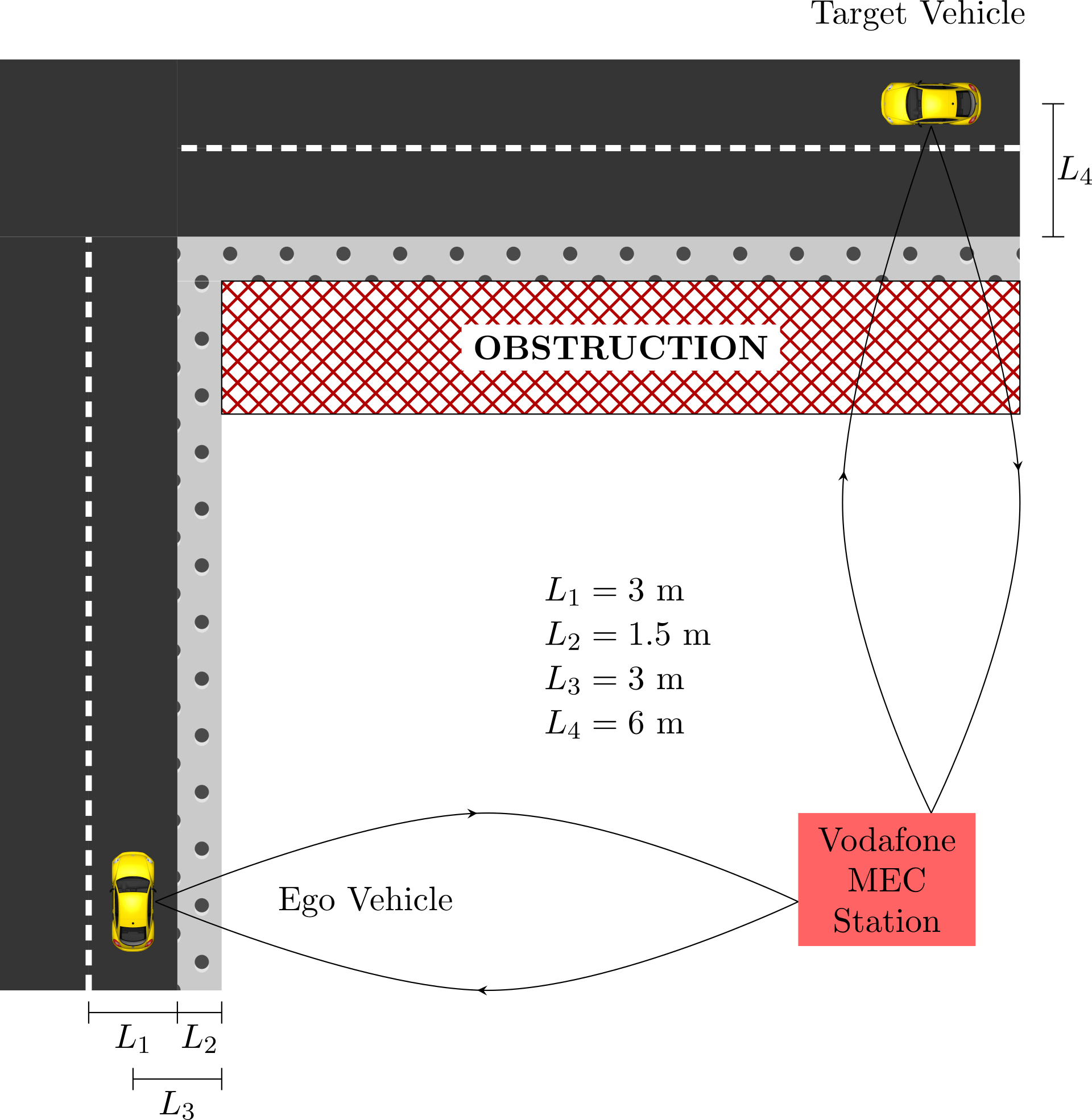
Figure 6: Scenario under consideration in the development of the AEB systems and their testing

It is important to note that the simplified setup was chosen for two main reasons:

• it is one of the most common intersection crashes schemes;

• it allows the work to concentrate on the power of connectivity and its potential influence on safety systems.

The scenario considered is a blind intersection where the initial velocity of the Target Vehicle is set to ensure that it crashes with the Ego Vehicle just before any braking takes place. It is also important to note that it is assumed that the Ego Vehicle, unlike the Target Vehicle, can be actuated.

4 IPG CarMaker/Simulink Implementation

IPG CarMaker is a tool for virtual testing of vehicles, which allows to recreate realistic test scenarios in a virtual environment. IPG CarMaker provides a Virtual Vehicle Environment (VVE), which consists of the virtual road, virtual driver, and virtual vehicle. Furthermore, IPG CarMaker has a user-friendly MATLAB/Simulink interface that facilitates modeling the connected system architecture, as seen in Figure 4.

4.1 Scheme of Connected Commercial System

The summary of the developed Simulink model for the two control logics is presented in Figure 7.

Figure 7: Summary of Developed System

4.1.1 Current System Model

As an initial step, the current system architecture (as modeled in Figure 2, and illustrated in 7) was modeled in IPG CarMaker.

For the perception block, information from the radars of the ego vehicle about surrounding visible vehicles was analyzed to determine whether to activate the TTC Calculation block or not (according to the activation criteria defined earlier).

For the purpose of this work, [14] and [28] are used to build the TTC calculation block in the Simulink model.

Figure 8: TTC in X-Y Plane

Figure 8 illustrates the setup for the calculation of the TTC, based on an a global X-Y reference frame. The equations can be easily adjusted to take into consideration that the radar gives information relative to the ego vehicle reference frame. The point at which the intersection can be given by the following expressions, given by Equations 4 and 5:

$$x_{+} =\dfrac{(y_{ego}-y_{target})-(x_{ego}\cdotp\tan\theta_{ego}-x_{target}\cdotp\tan\theta_{target})}{\tan\theta_{target}-\tan\theta_{ego}}$$ (4)

$$y_{+} =\dfrac{(x_{ego}-x_{target})-(y_{ego}\cdotp\cot\theta_{ego}-y_{target}\cdotp\cot\theta_{target})}{\cot\theta_{target}-\cot\theta_{ego}}$$ (5)

After finding the intersection point, the Time-to-Reach (TTR) values for each vehicle can be obtained by Equations 6 and 7:

$$\text{TTR}_{target} =\dfrac{\sqrt{(x_{+}-x_{target})^{2}+(y_{+}-y_{target})^{2}}}{v_{target}}$$ (6)

$$\text{TTR}_{ego} =\dfrac{\sqrt{(x_{+}-x_{ego})^{2}+(y_{+}-y_{ego})^{2}}}{v_{ego}}$$ (7)

To consider a more realistic case, it cannot be said that the vehicles will crash only when $\text{TTR}_{target}=\text{TTR}_{ego}$. Hence, it could be said that $\delta$ is a safety parameter described by Equation 8, such that:

$$\text{TTC}=\begin{cases}\min(\text{TTR}_{target},\text{TTR}_{ego})&\text{if}\ |\text{TTR}_{target}-\text{TTR}_{ego}|\leq\delta\\ \text{NaN}&\text{else}\end{cases}$$ (8)

To achieve similar performance between the simulated system and the reference real one provided by our partners, an expression of $\delta$ as a function of speed was reached by tuning the system to achieve the results described in Figure 9b and Figure 10b. In the latter figures, the green square means that the collision was avoided using the radar AEB logic, and the red square means that a collision occurred. The tuning of $\delta$ was done taking into consideration speeds of vehicles that yield the following collision configurations during the braking process, as seen in Figure 11.

It is important to note that the AEB logic is a temporal one. Hence, it required a FSM finite state machine implemented by means of Stateflow on MATLAB.

(a) Open Field Scenario

(b) Open Field Results

Figure 9: Description of Open Field Case

(a) Obstructed Field Scenario

(b) Obstructed Field Results

Figure 10: Description of Obstructed Field Case

Figure 11: Different Collision Configurations

The acceleration controller block is PI controller that provides as an output a value of the required brake pedal (between $0$ and $1$) to achieve a certain deceleration value. It is important to note that the acceleration controller module is activated only when the AEB is taking place. The development of this ACC is based on work presented in [29]. It is important to note that for our work, it is required that the driver can no longer press the gas when the AEB takes into action.

Figure 12: Acceleration Control Architecture

Figure 12 shows the longitudinal acceleration controller. The architecture of the controller can be described as: Discrete PI Controller with Integral Anti-Windup. The control signal is calculated using the backward Euler discretization method [31] (where the gains were tuned), as given by Equations 9 and 10:

$$u(k)=\text{sat}(p_{\text{gain}}\Delta a_{x}+\text{sat}(i_{\text{gain}}\frac{T_{s}z}{z-1}\Delta a_{x},A,B),A,B)$$ (9)

$$\text{sat}(x,A,B)=\min(\max(x,A),B)$$ (10)

Where:

$p_{\text{gain}}$ ${}={}$	0.001
$i_{\text{gain}}$ ${}={}$	0.001
$Ts$ ${}={}$	0.001 s
$A$ ${}={}$	Lower Limit of Saturation (1)
$B$ ${}={}$	Upper Limit of Saturation (0)

4.1.2 Connected System Model: Type A

The connected system architecture shown in Figure 4 was reached by making modifications to the previously developed Simulink model to take into consideration information from GPS, 5G, and Pirelli Cyber Tyre. It is important to note that the activation criteria remains the same for both the radar and 5G systems, as it is a characteristic of the type of collision the system is aimed at avoiding.

Concerning 5G communications characteristics, literature suggests that the maximum value of delay accepted for this kind of applications is $10$ ms. This guarantees the minimum safety requirements [27]. The exact characteristics of the 5G network provided by Vodafone were used in the development; however, they could not be mentioned here for confidentiality purposes.

Concerning the GPS information, CarMaker allows the modeling of the following errors [29, 30]:

• Receiver Clock Error: Arises because the receiver clock is not always synchronized with that of satellites. Standard deviation $=5$ m with Correlation time $=3600$ ms.

• Ephemeris Error or Orbit Error: Arises because of the small variations of the orbits of travel of the GPS satellites. Standard deviation $=3$ m with Correlation time $=1800$ ms.

• Ionospheric Delay: Arises because of ions in the ionosphere. Standard deviation $=5$ m with Correlation time $=3600$ ms.

• Tropospheric Delay: Arises because of the refractions of the signal due to the variations of atmospheric conditons. Standard deviation $=2$ m with Correlation time $=1800$ ms.

• Receiver Noise: Pseudorange $=0.1$ m, and Rated range = $0.05$ m

Cocerning the Pirelli Cyber Tyre, it was mentioned earlier that it is able to provide information about the potential friction after braking takes place. Hence, the use of this information is not optimal for the commercial braking logic, as it is a static velocity-dependent logic. For example, even if the potential ground friction was measured to be low while braking is taking place, nothing can be done about it. Considering the current AEB logic, it is clearly seen that the nature of the logic prohibits utilizing the Ego Vehicle’s Pirelli Cyber Tyre to its full potential.

As an initial attempt to utilize information about potential ground friction, it is assumed that it is available from an active map. This assumption is realistic, for example, in a scenario where several vehicles are driving in the same area and sharing their potential ground friction estimation that is so collected in an active map available to the ego vehicle. For this reason, it was reasonable to include braking distance in the logic. The scheme is shown in Figure 13. Now, the trigger to the system is no longer the TTC only, but also the braking distance. If the braking distance becomes equal to a certain threshold related to the distance to the collision point, the braking maneuver takes place.

Figure 13: Detailed Scheme of Upgraded System A

It is noteworthy that the parameters of the braking logic weren’t modified: this first novel approach assumed that the ECU containing the AEB logic can’t be modified. In fact, this approach can be considered as an add-on with respect to the commercial configuration with the minimum modification required. The braking distance is calculated based on a the braking scheme originally described in Figure 3. The maximum deceleration level was modified based on the potential ground friction measurement, as described in Figure 14, and then the braking distance was calculated by performing numerical integration.

Figure 14: Modification of Braking Scheme

It could be seen that the scheme provided in Figure 13 complies with the system architecture provided in Figure 4. Here, information coming from 5G about the position ad speed of nearby vehicles is used to evaluate TTC, and the BD based on the received potential ground friction. Once either one of the triggers is activated, a deceleration request is sent to the acceleration controller.

4.1.3 Connected System Model: Type B

This approach means a deeper modification of the vehicle original hardware and software configuration in order to obtain better results in terms of safety. In an attempt for further development, it was decided to modify the braking logic block. This is because the current braking logic does not facilitate taking advantage of the potential of he information received from the Pirelli Cyber Tyre. It is important to explore the option of giving the vehicle a reference deceleration that is adaptable to the road conditions: for example: increases exponentially throughout the braking maneuver. This approach tries to mimic the commercial braking logic, in that the braking logic requests an initial deceleration value of around $30\%$ of the maximum possible deceleration, and reaches $80\%$ of its maximum value (this allows the driver to still have control on the vehicle at maximum braking). The formulation is given by Equation 11:

$$a(t)=Ae^{\alpha t}$$ (11)

Where $A=-\max\ (k_{\text{min}}\mu g,a_{\text{current}})$. The velocity profile is given by Equation 12:

$$v(t) =v_{0}+\int_{0}^{t}a(t)\text{d}t$$ (12)

$$=v_{0}+\frac{A}{\alpha}e^{\alpha t}-\frac{A}{\alpha}$$

The displacement of the vehicle is given by Equation 13:

$$s(t) =\int_{0}^{t}v_{0}+\frac{A}{\alpha}e^{\alpha t}-\frac{A}{\alpha}\ \text{d}t$$ (13)

$$=\frac{A}{\alpha^{2}}e^{\alpha t}+Bt+C$$

Now, it is considered that the vehicle must reach a complete stop at time $T$ ($v(T)=0$), such that $a(T)\leq-a_{\text{max}}\mu g$ and $s(t)\leq d$, where $d$ is the distance to the intersection. Due to complex nature of the problem, the following approach was considered, as seen in Figure 15:

Figure 15: Detailed Scheme of Upgraded System B

At every loop, the trigger block solves the following to get values of $\alpha$ and $T$:

$$v(T)=0,\ s(T)=d$$

Once the values of $\alpha$ and $T$ are obtained, $a(T)=Ae^{\alpha T}$ is calculated. If $a(T)\geq a_{\text{max}}\mu g-a_{\text{tuned}}$ (where $a_{\text{tuned}}$ is a certain threshold that is tuned, for our case it is $1\ \text{m}/\text{s}^{2}$), then the trigger is activated and the braking maneuver is initiated.

It could be immediately seen that the system still has an issue with the characteristic of the Pirelli Cyber Tyre (since it provides an estimate of the value of potential ground friction at the moment of braking). However, the advantage here is that the system is somehow adaptable, providing a higher deceleration value as a compensation. The adaptability of the system is highly affected by the value of $a_{\text{tuned}}$.

5 Simulation Testing Results

5.1 Upgraded System Type A: Normal Ground Friction Environment

The test was carried out with a ground friction coefficient equal to $0.85$ . The test results displayed are for the case when both vehicles approach the intersection traveling at 60 km/h. It is noteworthy that the system was tested for all velocity combinations as outlined in Figure 10b. However, as a choice of displaying results in this paper, the case of having both vehicles traveling at high velocities was chosen, as it is usually the case causing collision without connectivity as well as with low ground friction. The modified system was tested in a normal friction conditions, as seen in Figure 16. It could be clearly seen in 17a that the maximum deceleration a vehicle can reach in normal ground friction conditions is approximately $8.3\text{m/s${}^{2}$}$.

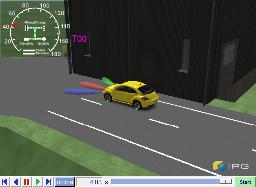
(a)

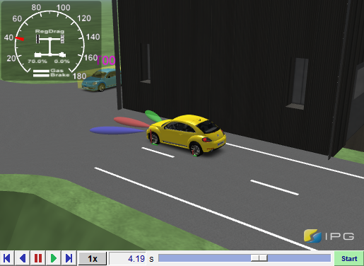
(b)

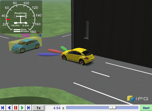
(c)

Figure 16: Screenshots from CarMaker in Chronological Order: System Type A, Normal Ground Friction

From Figure 16 it could be seen that the vehicle avoids the collision. Also, the vehicle approaches the intersection at a reduced speed, and the stopping takes place before the pre-defined collision point; this is quite important as the AEB action turns off when the vehicle reaches a complete stop.

Relevant numerical results are presented in Figure 17.

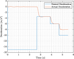
(a)

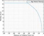
(b)

Figure 17: System Type A: Normal Ground Friction, (a) Desired Deceleration vs Actual Deceleration (b) Ego Vehicle Velocity vs Distance to Collision Point

Figure 17a shows the deceleration request as well as the actual one. Note that the value of $-15$ $\text{m}/\text{s}^{2}$ is the equivalent of no deceleration request. It could be seen in Figures 17a and 17b that once the condition described in Equation 8 is satisfied, the AEB system is activated.

5.2 Upgraded System Type A: Low Ground Friction Environment

The modified system was tested in a low friction condition ($\mu=0.4$).

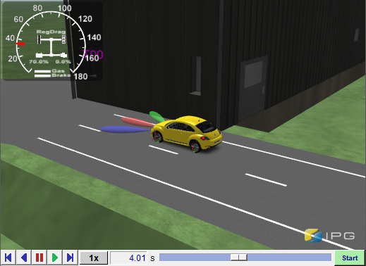
(a)

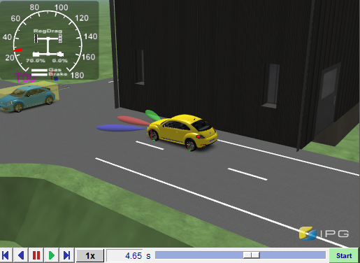
(b)

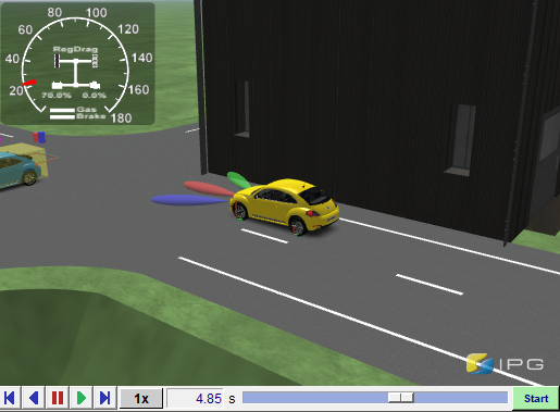
(c)

Figure 18: Screenshots from CarMaker in Chronological Order: System Type A, Low Ground Friction

Relevant numerical results are presented in Figure 19.

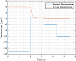
(a)

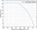
(b)

Figure 19: System Type A: Low Ground Friction, (a) Desired Deceleration vs Actual Deceleration (b) Ego Vehicle Velocity vs Distance to Collision Point

From Figure 18 it could be seen that the vehicle avoids the collision. Also, the vehicle approaches the intersection at a reduced speed, and the stopping takes place before the pre-defined collision point. Furthermore, comparing Figures 17b and 19b, it could be seen that in low ground friction, the braking starts 34 meters and 44 meters before the predicted collision point, respectively.

It could be seen in Figure 19a that the vehicle is unable to reach the deceleration requested as a result of the ground condition.

It is clear that the only way for the system to avoid the collision in this case is activating the AEB system earlier thorough the braking distance calculation which utilizes a priori knowledge about ground friction. The difference could be clearly seen when comparing Figure 17b and Figure 19b.

5.3 Upgraded System Type B: Normal Ground Friction Environment

(a)

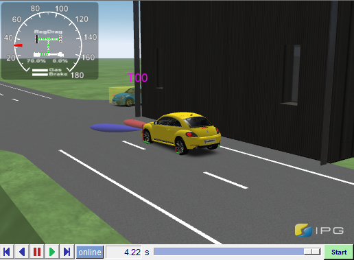
(b)

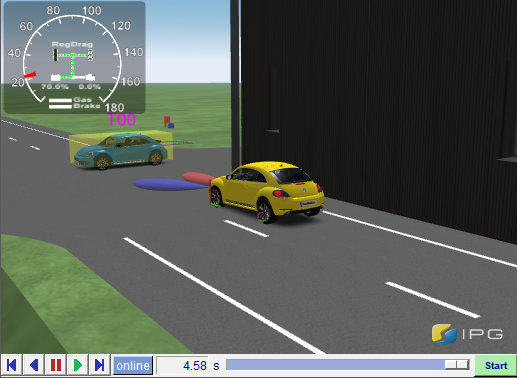
(c)

Figure 20: Screenshots from CarMaker in Chronological Order: System Type B, Normal Ground Friction

Relevant numerical results are presented in Figure 21. It could be seen from Figure 21a that the braking maneuver follows an exponential deceleration scheme. Hence, with respect to the stepped scheme in System A, System B provides a smoother profile that reflects an improvement in driving comfort.

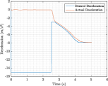
(a)

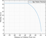
(b)

Figure 21: System Type B: Normal Ground Friction, (a) Desired Deceleration vs Actual Deceleration (b) Ego Vehicle Velocity vs Distance to Collision Point

When inspecting Figure 20, it could be seen that the vehicle successfully avoids the collision. Also, the vehicle stops completely before the collision point.

5.4 Upgraded System B: Low Ground Friction Environment

5.4.1 Friction Known A Priori

It would be interesting to investigate the case where the low ground friction value ($\mu=0.4$) is known before the braking maneuver takes place.

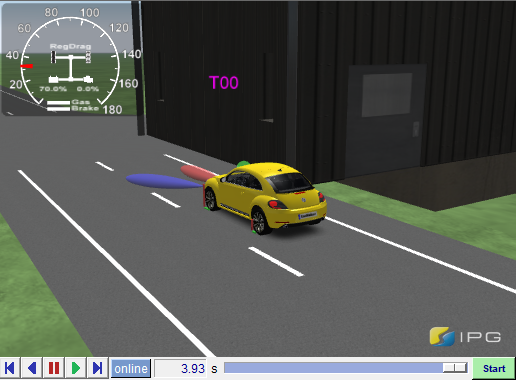
(a)

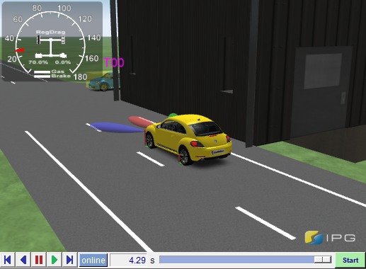
(b)

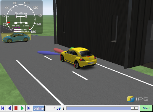
(c)

Figure 22: Screenshots from CarMaker in Chronological Order: System Type B, Low Ground Friction

Relevant numerical results are presented in Figure 23. It could be seen that the vehicle successfully stops before the intersection, and avoids the collision. It could be seen from Figure 23a that the braking maneuver is smooth and comfortable. When comparing the performance of System B in low friction with that of System A (Figure 19a), it could be seen that the system manages to stop further away from the intersection. On the other hand, the tunability of System B allows the vehicle to be more under control (steerable) since the maximum value of deceleration requested can be set well below the friction limit.

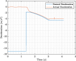
(a)

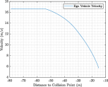
(b)

Figure 23: System Type B: Low Ground Friction, (a) Desired Deceleration vs Actual Deceleration (b) Ego Vehicle Velocity vs Distance to Collision Point

5.4.2 Friction Retrieved from an Active Map

In this last case, a more realistic scenario is presented. Considering the presence of an active map containing inaccurate ground friction estimates (due to several possible factors such as old data, measurements errors, …). The value provided by the map ($\mu=0.6$) is higher than the real value ($\mu=0.4$).

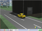
(a)

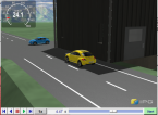
(b)

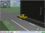
(c)

Figure 24: Screenshots from CarMaker in Chronological Order: System Type B, Low Ground Friction

Relevant numerical results are presented in Figure 25.

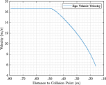
(a)

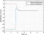
(b)

Figure 25: System Type B: Low Ground Friction,(a) Desired Deceleration vs Actual Deceleration (b) Ego Vehicle Velocity vs Distance to Collision Point

It could be seen that with respect to the latter situation (as in Figure 23a), the system starts braking later. However, the maximum possible deceleration is reached as fast as possible to ensure that the collision is avoided. It could be seen that the safety is improved as the system is now more adaptive to the environmental conditions.

6 Conclusion

To conclude, the aim of this work was the following:

• develop and test two novel intersection collision avoidance systems that rely on information from 5G, radar sensors, and Pirelli CyberTyre;

• test the usability of 5G in safety systems of connected vehicles.

As presented in the paper, state of the art AEB systems usually issue a predefined braking request based on a static trigger. The advantage of such existing systems is the simplicity which reflects the simple hardware and reduced costs. Starting from these consideration, a novel approach consisting of an upgrade of the original architecture in order to limit costs of the design of new hardware and software, is presented. While keeping the same braking logic adopted in the radar system, an additional trigger was added to enable braking based on braking distance. The results of the virtual testing have been positive in both normal ground friction and low ground friction environments. In order to fully take advantage of the ground friction estimate, a second novel AEB control logic able to adapt itself during the braking is proposed. In detail, a braking scheme with an exponential-scheme was adopted as it ensures smooth braking as well as high robustness and adaptability to road conditions as shown by virtual simulations and comparison to the previous AEB proposed. However, due to the complex nature of the equations to be solved (to find $T$ and $\alpha$), the system requires much higher computational power. Also, the tuning of the parameter $a_{\text{tuned}}$ presents a disadvantage, as setting a high value will make the system start braking very early but the system will be more robust, and setting it very low will make system start braking at normal time but this will limit robustness.

Disclosure statement

The author(s) declared no potential conflicts of interest with respect to the research, authorship, and/or publication of this article.

Funding

The author(s) disclosed receipt of the following financial support for the research, authorship, and/or publication of this article: This work has been supported by Vodafone Italia under Vodafone 5G Trial in Milan.

References

- World Health Organization [2018] W. H. Organization, Global Status Report on Road Safety 2018. World Health Organization, 2018.
- Lombardi, Horrey, and Courtney [2017] D. A. Lombardi, W. J. Horrey, and T. K. Courtney, “Age-related Differences in Fatal Intersection Crashes in the United States,” Accident Analysis & Prevention, vol. 99, pp. 20–29, 2017.
- Sanders and Lubbe [2018] U. Sander and N. Lubbe, “Market Penetration of Intersection AEB: Characterizing Avoided and Residual Straight Crossing Path Accidents,” Accident Analysis & Prevention, vol. 115, pp. 178–188, 2018.
- Scanlon et al. [2017] J. M. Scanlon, R. Sherony, and H. C. Gabler, “Injury Mitigation Estimates for an Intersection Driver Assistance System in Straight Crossing Path Crashes in the United States,” Traffic injury prevention, vol. 18, no. sup1, pp. S9–S17, 2017.
- Euro NCAP [2015] N. Euro, “Euro NCAP 2020 Roadmap,” Leuven, Belgium, 2015.
- Sanders and Lubbe [2018] U. Sander and N. Lubbe, “The Potential of Clustering Methods to Define Intersection Test Scenarios: Assessing Real-life Performance of AEB,” Accident Analysis & Prevention, vol. 113, pp. 1–11, 2018.
- Saffarzadeh et al. [2013] M. Saffarzadeh, N. Nadimi, S. Naseralavi, and A. R. Mamdoohi, “A General Formulation for Time-to-collision Safety Indicator,” in Proceedings of the Institution of Civil Engineers-Transport, vol. 166, no. 5. Thomas Telford Ltd, 2013, pp. 294–304.
- Eichhorn et al. [2013] A. von Eichhorn, P. Zahn, and D. Schramm, “A Warning Algorithm for Intersection Collision Avoidance,” in Advanced Microsystems for Automotive Applications 2013. Springer, 2013, pp. 3–12.
- Wu et al. [2018] X. Wu, L. N. Boyle, D. Marshall, and W. O’Brien, “The Effectiveness of Auditory Forward Collision Warning Alerts,” Transportation research part F: traffic psychology and behaviour, vol. 59, pp. 164–178, 2018.
- Lee et al. [2002] J. D. Lee, D. V. McGehee, T. L. Brown, and M. L. Reyes, “Collision Warning Timing, Driver Distraction, and Driver Response to Imminent Rear-end Collisions in a High-fidelity Driving Simulator,” Human factors, vol. 44, no. 2, pp. 314–334, 2002.
- Lee et al. [2004] J. D. Lee, J. D. Hoffman, and E. Hayes, “Collision Warning Design to Mitigate Driver Distraction,” in Proceedings of the SIGCHI Conference on Human factors in Computing Systems. ACM, 2004, pp. 65–72.
- Yang [2013] J. Yang, “A Vehicle Intersection Collision Warning System using Smartphones,” Ph.D. dissertation, University of Massachusetts Lowell, 2013.
- Berthelot [2011] A. Berthelot, A. Tamke, T. Dang, and G. Breuel, “Handling Uncertainties in Criticality Assessment,” in 2011 IEEE Intelligent Vehicles Symposium (IV).IEEE, 2011, pp. 571–576.
- Miller and Huang [2002] R. Miller and Q. Huang, “An Adaptive Peer-to-peer Collision Warning System,” in Vehicular Technology Conference. IEEE 55th Vehicular Technology Conference. VTC Spring 2002 (Cat. No. 02CH37367), vol. 1. IEEE, 2002, pp. 317–321.
- Kim et al. [2015] E.-S. Kim, S.-K. Min, D.-H. Sung, S.-M. Lee, and C.-B. Hong, “The AEB System with Active and Passive Safety Integration for Reducing Occupants’ Injuries in High-Velocity Region,” in 24th International Technical Conference on the Enhanced Safety of Vehicles (ESV) National Highway Traffic Safety Administration, no. 15-0335, 2015.
- Choo et al. [2014] H. Cho, G.-E. Kim, and B.-W. Kim, “Usability Analysis of Collision Avoidance System in Vehicle-to-vehicle Communication Environment,” Journal of Applied Mathematics, vol. 2014, 2014.
- Jeon et al. [2016] S. Jeon, D. G. Lee, and B. Kim, “Improved AEB Performance at Intersections with Diverse Road Surface Conditions Based on V2V Communication,” in Advanced Multimedia and Ubiquitous Engineering. Springer, 2016, pp. 219–224.
- Kapse and Adarsh [2019] R. Kapse and S. Adarsh, “Implementing an Autonomous Emergency Braking with Simulink using two Radar Sensors,” arXiv preprint arXiv:1902.11210, 2019.
- Tamke et al. [2011] A. Tamke, T. Dang, and G. Breuel, “A Flexible Method for Criticality Assessment in Driver Assistance Systems,” in 2011 IEEE Intelligent Vehicles Symposium (IV). IEEE, 2011, pp. 697–702.
- Lee et al. [2014] D. Lee, S. Kim, C. Kim, and K. Huh, “Development of an Autonomous Braking System using the Predicted Stopping Distance,” International Journal of Automotive Technology, vol. 15, no. 2, pp. 341–346, 2014.
- Seiler et al. [1998] P. Seiler, B. Song, and J. K. Hedrick, “Development of a Collision Avoidance System,” SAE transactions, pp. 1334–1340, 1998.
- Doi et al. [1994] A. Doi, T. Butsuen, T. Niibe, T. Takagi, Y. Yamamoto, and H. Seni, “Development of a Rear-end Collision Avoidance System with Automatic Brake Control,” Jsae Review, vol. 15, no. 4, pp. 335–340, 1994.
- Fujita et al. [1995] Y. Fujita, K. Akuzawa, and M. Sato, “Radar Brake System,” Jsae Review, vol. 1, no. 16, p. 113, 1995.
- Malinverno et al. [2018] M. Malinverno, G. Avino, C. Casetti, C.-F. Chiasserini, F. Malandrino, and S. Scarpina, “Performance Analysis of C-V2I-based Automotive Collision Avoidance,” in 2018 IEEE 19th International Symposium on” A World of Wireless, Mobile and Multimedia Networks”(WoWMoM). IEEE, 2018, pp. 1–9.
- Amjad et al. [2018] Z. Amjad, A. Sikora, J.-P. Lauffenburger, and B. Hilt, “Latency reduction in narrowband 4g lte networks,” in 2018 15th International Symposium on Wireless Communication Systems (ISWCS). IEEE, 2018, pp. 1–5.
- Fettweis et al. [2014] G. Fettweis, H. Boche, T. Wiegand, E. Zielinski, H. Schotten, P. Merz, S. Hirche, A. Festag, W. Häffner, M. Meyer et al., “The tactile internet-itu-t technology watch report,” Int. Telecom. Union (ITU), Geneva, 2014.
- 5GAA [2019] 5GAA, “C-V2X Use Cases: Methodology, Examples and Service Level Requirements,” Tech. Rep., 07 2019.
- Jiménez et al. [2013] F. Jiménez, J. E. Naranjo, and F. García, “An Improved Method to Calculate the Time-to-Collision of Two Vehicles,” International Journal of Intelligent Transportation Systems Research, vol. 11, no. 1, pp. 34–42, 2013.
- IPG Automotive [2018] IPG Automotive, “User’s Guide,” IPG Automotive, 2018.
- IPG Automotive [2018] IPG Automotive, “Reference Manual,” IPG Automotive, 2018.
- Lee [1992] D. Lee, “IEEE Recommended Practice for Excitation System Models for Power System Stability Studies (IEEE Std 421.5-1992),” Energy Development and Power Generating Committee of the Power Engineering Society, vol. 95, no. 96, 1992.