Size Matters

Abstract

Fully convolutional neural networks can process input of arbitrary size by applying a combination of downsampling and pooling. However, we find that fully convolutional image classifiers are not agnostic to the input size but rather show significant differences in performance: presenting the same image at different scales can result in different outcomes. A closer look reveals that there is no simple relationship between input size and model performance (no ‘bigger is better’), but that each each network has a preferred input size, for which it shows best results. We investigate this phenomenon by applying different methods, including spectral analysis of layer activations and probe classifiers, showing that there are characteristic features depending on the network architecture. From this we find that the size of discriminatory features is critically influencing how the inference process is distributed among the layers.

1 Introduction

The relation between the neural architecture and the resolution of the input image is an often overlooked property of convolutional neural network (CNN) classifier. Early designs like Krizhevsky et al. (2012); Simonyan & Zisserman (2014) and Szegedy et al. (2015) chose square resolutions between $224\times 224$ and $299\times 299$ pixels mainly as a compromise between image size and computational efficiency. In recent publications like Huang et al. (2018) the resolution is increased up to $600\times 600$ pixels.

Furthermore Tan & Le (2019) show experimentally that the input resolution increases the performance reliably on various architectures. The intuitive explanation offered by authors like Szegedy et al. (2016) for this phenomenon is the addition of greater detail gained by increasing the size of the image. These details potentially yield additional features that can be detected by the classifier, resulting in higher performance.

Tan & Le (2019) introduces also the idea that the size of the input image needs to match the neural architecture for optimal efficiency and performance; they use the size of the input image as one of 3 linearly related properties for scaling up neural network architectures.

1.1 Contribution

In this work we investigate the following questions addressing the relationship between input size and model architecture:

• Has the size of the input image an effect on the predictive performance of CNN classifiers? Answer: yes, it is shown that not just increasing the amount of details but just altering the image resolution can improve classification accuracy (Section 3.1).

• Does the size of the input image influence how the information is processed in the network? Answer: yes, we can show that processing significantly differs depending on input size (Section 3.2) and the size of the depicted objects (Section 3.3).

• Can we know in advance which layers will contribute to the quality of the prediction based on the input size? Answer: For strictly sequential architectures the receptive field size allows to identify unproductive layers (Section 3.4).

• Do residual connections influence the observed behavior? Yes, residual connections can help to involve more layers in the inference process (Section 3.5).

2 Background

2.1 Fully Convolutional Networks

This work focuses on fully convolutional neural network classifiers; the current de facto standard for CNN classifier architectures (He et al., 2015; Szegedy et al., 2016; Tan & Le, 2019; Iandola et al., 2014). While convolution is a local operation that can in principle deal with input of arbitrary height and width, the fully connected dense layers used for the output operate globally and hence enforce specific input and output shapes. Therefore architectures such as AlexNet have a fixed input size and require changes to the architecture in order to change the input size (Krizhevsky et al., 2012). In contrast, fully convolutional networks only apply a stack of convolutional filters to the input, resulting in feature maps whose size depends on the size of the input data. These feature maps can be summarized, usually by global average pooling, to obtain a feature vector of fixed dimensionality that can be used for further processing, e.g. classification (Szegedy et al., 2016). This makes fully convolutional neural networks effectively agnostic to the size of the input.

Being able to change the size of the input image without altering the architecture of the CNN is important for avoiding potential artifacts induced by architectural changes. For this reason we also modify non-fully convolutional architectures such as the VGG-family of networks by Simonyan & Zisserman (2014) to be fully convolutional. This is done by simply replacing the readout, which reshapes the tensor produced by a convolutional layer into a vector by a global average pooling layer (Lin et al., 2013).

2.2 Probe Classifiers

Probe classifiers were initially proposed by Alain & Bengio (2016) as a tool for analyzing how the solution quality progresses while the data is propagated through neural networks. In order to do this, logistic regression ”probes” are trained on the same task as the model, using the output of individual layers from the trained model as input. Since the softmax layer and a cross-entropy minimizing logistic regression effectively solve the same task, we can use these probes to see how the quality of the intermediate solution evolves during the forward pass. Usually, probe accuracy will be low for the first layers and increase throughout the network to approximate the model accuracy in the final layers, as the example shown in figure 1 demonstrates.

2.3 Saturation and Tail Patterns

Saturation is another technique for expressing the activity of a neural network layer in a single number, introduced by Richter et al. (2020). The saturation metric of a layer is obtained by computing the number of eigendirections in the output required to explain 99% of the total variance and dividing this number by the dimensionality of the layer’s output. Similar to the accuracy of a probe classifier, this results in a value bound between 0 and 1. Intuitively saturation measures a percentage of how much the output space of a layer is “filled” or “saturated” with the data. Richter et al. (2020) show that interesting patterns can be observed when the saturation of every layer is plotted in sequence of the forward pass. Important for our work is the “tail pattern”, which can be seen in figure 1, as it indicates an inefficiently distributed forward pass.

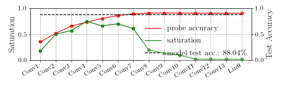
(a)

Figure 1: VGG16 trained on Cifar10 with $32\times 32$ pixel input size. The model exhibits a tail pattern starting from Conv8. Note that the probe performance in the tail is roughly equal to the performance of the model itself.

A tail pattern is a sub-sequence of layers, generally found close to the input or the output of the network, with significantly less saturation than all other layers. By observing probe performances we find that these layers generally do not contribute significantly to the inference process by devolving to quasi-pass-through layers over the course of training. We will refer to these layers as unproductive layers or unproductive sequences.

2.4 The receptive field size

The receptive field size is a property of a convolutional layer inside a neural network architecture. The receptive field size describes the maximum height and width of a square area on an arbitrarily large input image. Only pixels contained in this area may influence the output of a single convolution operation. In other words, the receptive field size describes the spatial upper bound of visual patterns detectable by the respective layer.

For convolutional neural networks with a sequential structure (no multiple pathways during the forward pass) the receptive field size can be computed analytically. We refer to the receptive field $r$ of the $l$th layer of sequential network structure as $r_{l}$ (with $r_{0}=1$, which is the ”receptive field” of the input). For all layers $l>0$ in the convolutional part of a sequential network the receptive field can be computed with the following formula:

$$r_{l}=r_{l-1}+((k_{l}-2)\prod^{l-1}_{i=0}s_{i})$$ (1)

where $r_{l-1}$ is the receptive field of the previous layer, $k_{l}$ refers to the kernel size of layer $l$ (with potential dilation already accounted for) and $s_{i}$ the stride size of layer $i$. In the simplest case, which is the first convolutional layer of the neural architecture, $r_{1}$ is exactly the size of the kernel. When convolutional layers are stacked, the receptive field expands for every layer $l$ with a kernel size $k_{l}\neq 1$. The stride size $s_{l}$ of a layer $l$ furthermore has a multiplicative effect on the growth rate of the receptive field, since a stride effectively downsamples the feature map.

While the ResNet-family of networks by He et al. (2015) is not strictly sequential due to their residual connections, we compute the receptive field size by simply ignoring the residual connections. We can do this in the context of this work because residual connections do not change the receptive field size and we are only interested in the receptive field size as a spatial upper bound for the integration of information into single output positions.

2.5 Choice of Models

The experiments are primarily conducted on VGG and ResNet-style architectures originally developed by Simonyan & Zisserman (2014) and He et al. (2015).

The purpose of the VGG-style architectures in this work is to serve as a baseline of simple sequential CNN architectures. The VGG architectures are modified by using a global average pooling layer in the readout in order to make them fully convolutional. Furthermore we use variants that utilize batch-normalization after each layer, which has become a widespread pattern in many more recent architectures (He et al., 2015; Tan & Le, 2019; Huang et al., 2018).

For more complex architectures we choose the ResNet family and will mainly focus on ResNet18 for analysis in the main part of this work. The reason for this decision is two-fold. First, ResNet networks utilize many ideas of modern neural architectures, like the building block design and residual connections, while being rather simple in their structure (Tan & Le, 2019; Iandola et al., 2014; Szegedy et al., 2016). Second, the ResNet family and ResNet18 in particular are easy to visualize, while many more complex derivative architectures feature a more non-sequential structure and a much larger amount of consecutive layers, making the experimental results harder to read and interpret.

To demonstrate that the claims made in this work generalize we reproduce some results on additional models such as EfficentNet-B0, ResNet34 and ResNet50 and provide them either in the main part of this work or in the supplementary material.

2.6 Training Setup

Training on any dataset is conducted using a batch size of 64 (see supplementary material for more details). If no information on the input size is given it can be assumed that the native resolution of the dataset is fed into the network. The training data is augmented by random cropping, horizontal flipping and channel wise normalization of the data points using ImageNet computed means and standard deviations of every color channel. When images are resized linear interpolation is used and the resize is applied after data augmentation and any other preprocessing. We use the stochastic gradient decent optimizer for training. The learning rate is set initially to 0.1 and reduced after one and two thirds of the trained epochs by a factor 10. The models are trained for 30 epochs with the exception of ResNet50, which is trained for 60 epochs due to slow convergence. No hyperparameter optimization or fine tuning on hyperparameters is conducted, since it is not the goal of the paper to achieve maximum or state-of-the-art performance. We find that changing the learning rate, optimizer, batch size, data augmentation and number of epochs trained does not influence the conclusions of the experiments in any significant way as long as the model is able to converge to a solution better than chance-level (see supplementary material).

2.7 Datasets

Multiple datasets are used to conduct and verify the experiments presented in this work. Experiments that require small base images were conducted on Cifar10 and reproduced on MNIST and TinyImageNet (Le & Yang, 2015; Krizhevsky et al., 2010; LeCun & Cortes, 2010). Experiments requiring images of higher resolution were conducted on iNaturalist as well as ImageNet (Horn et al., 2017; Russakovsky et al., 2015).

3 Experiments

A series of experiments has been conducted to investigate the relationship of input size and model architecture. We first demonstrate that input size affects the predictive performance of models even though no additional information is added by scaling the images. We then explore this effect further by reproducing these results on Cifar10 and analyzing the saturation and probe performance. Based on these results we investigate the role of locality of discriminatory features in the image. Finally we discuss the role of the receptive field in these observations and analyze the influence of residual connections.

3.1 Image Size and additional Details have independent effects on the predictive performance

Tan & Le (2019) showed that increasing the input resolution of a model leads to increased performance. The intuitive explanation for this effect is that adding details (i.e. information) leads to better performance. The working hypothesis is that more details is the only factor increasing performance when increasing the image size. We investigate by increasing the image size, with or without added detail.

We train multiple models on ImageNet and iNaturalist in three different settings A, B and C. Models of set A, are trained on images of the original design size of $224\times 224$ pixels, providing the performance baseline. Set B models are trained on images of size $32\times 32$. We expect the relative performance of these models to drop significantly in all scenarios, since the image detail is reduced. The third set of models C is trained on images that are first resized to $32\times 32$ pixels; then up-sampled to $224\times 224$ pixels. These images have as much detail as the images used for training the models of set B while keeping the larger size used for training the models of set A. According to the working hypothesis, performance should not increase relative to groups two.

Table 1: Relative Top1-Accuracy: The table shows the predictive performance of trained models relative to a baseline model. The baseline uses the same model and architecture and is trained on images resized to $224\times 224$ pixels. Training the models on $32\times 32$ pixel images results in less than half the predictive performance in all tested scenarios relative to the baseline. Resizing the $32\times 32$ images back to $224\times 224$ results in a significant recovery of lost performance in all tested scenarios, despite no information is added by upscaling.

Model	Dataset	downscaled	upscaled
		$32\times 32$	$224\times 224$
VGG16	ImageNet	15.35%	66.08%
VGG16	iNaturalist	36.83%	58.38%
ResNet18	ImageNet	45.74%	67.39%
ResNet18	iNaturalist	30.4%	52.68%
ResNet50	ImageNet	28.21%	71.8%
ResNet50	iNaturalist	33.87%	54.38%
EfficientNet-B0	ImageNet	19.32%	64.45%
EfficientNet-B0	iNaturalist	15.34%	63.79%

While performance suffers drastically when reducing the input size, we can also see in table 1 that decreasing, then increasing the image size regains some of the lost performance with all models. Based on this observation we can conclude that the size of the input images has an independent effect on the predictive performance. This also confirms observations made by Richter et al. (2020), were the same effect was observed on the Food101 dataset.

3.2 Input size affects the inference process of the CNN

To further understand what effect the input size has on the trained model and its performance, we train the same models on Cifar10. Cifar10 has a native resolution of $32\times 32$, therefore no additional details can be added by increasing the size of the image. We train ResNet18 on Cifar10s native resolution as well as $224\times 224$ pixels. We also train the model a third time using an input size of $1024\times 1024$ pixels, to understand what happens when the image is drastically oversized.

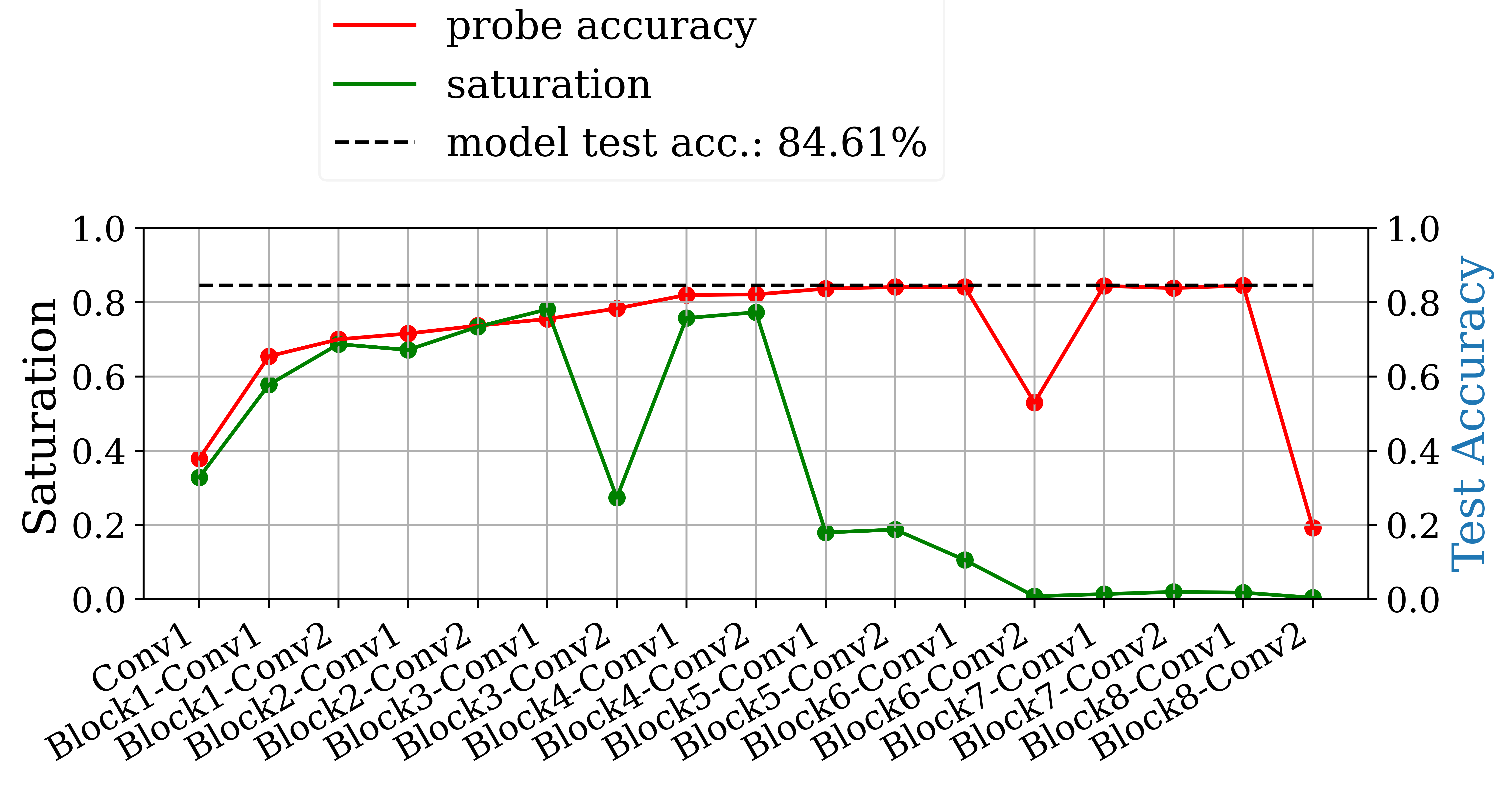
(a) $32\times 32$ (Cifar10 native resolution)

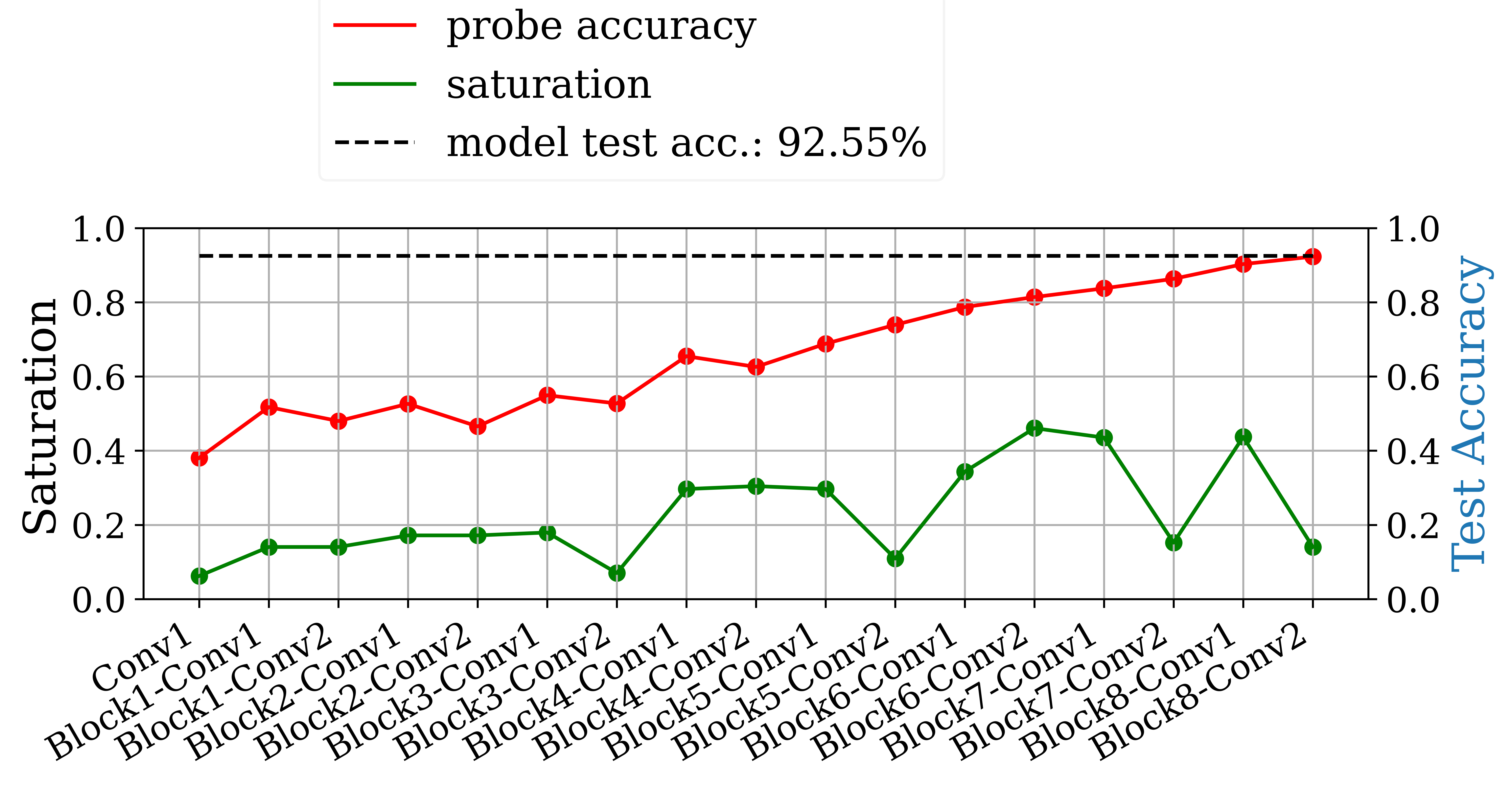
(b) $224\times 224$ (ResNet standard)

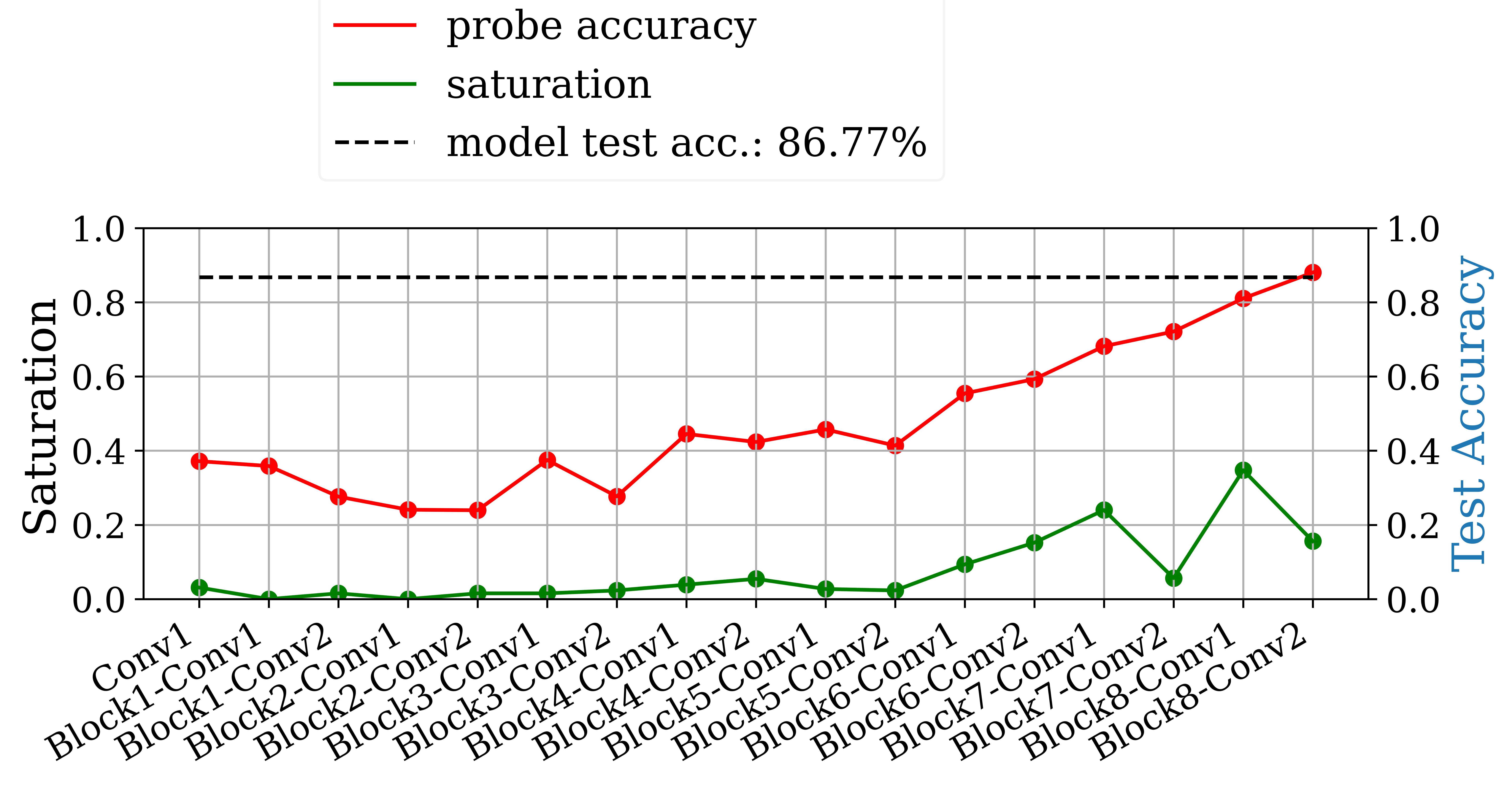
(c) $1024\times 1024$

Figure 2: Changing the input size changes how the inference is distributed among the layers. The resolution ResNet18 was designed for (b) distributes the inference most evenly, while too small (a) and too large (c) resolution shift the bulk of the inference process to early and later layers respectively, resulting in worse predictive performance.

The results in figure 2 show that the inference process is distributed differently among the layers depending on the input size. Best predictive performance is achieved at $224\times 224$, where inference is also distributed most evenly. At a substantially smaller size of $32\times 32$ pixels, the performance suffers, dropping from 92.79% accuracy to 84.64%. We also observe in figure 2a that only the first (highly saturated) two thirds of the network improve the predictive performance of the probes substantially from layer to layer. The rest of the network is lower saturated and does not contribute to improving the quality of the solution. Thus shrinking the input size has shifted the bulk of the qualitative inference process to the front of the network. Similarly, when drastically increasing the resolution to $1024\times 1024$ pixels (see figure 2c), the opposite effect can be observed. The qualitative inference process is shifted closer to the output, while the first half of the network does not substantially improve the predictive performance. The impact on the predictive performance is also negative, reducing the accuracy from 92.79% to 86.77% compared to the model trained on $224\times 224$ pixel input images.

3.3 The role of the object size in the relation of model and input resolution

Processing similar features with different sizes is a common challenge in the related field of object detection, where objects may strongly vary in size and position on the image (Redmon et al., 2015; Redmon & Farhadi, 2016, 2018; Bochkovskiy et al., 2020). One possible solution is the pyramid network concept introduced in (Han et al., 2016), which is also employed in popular models like YoloV3 by Redmon & Farhadi (2018). By utilizing feature maps from different parts of the network the model becomes more stable when the object size varies significantly. This indicates that processing objects of different size is handled by different parts of the network. Based on our previous observations, we hypothesize that the uneven distribution of the inference is caused by the size of features on the images used for classification.

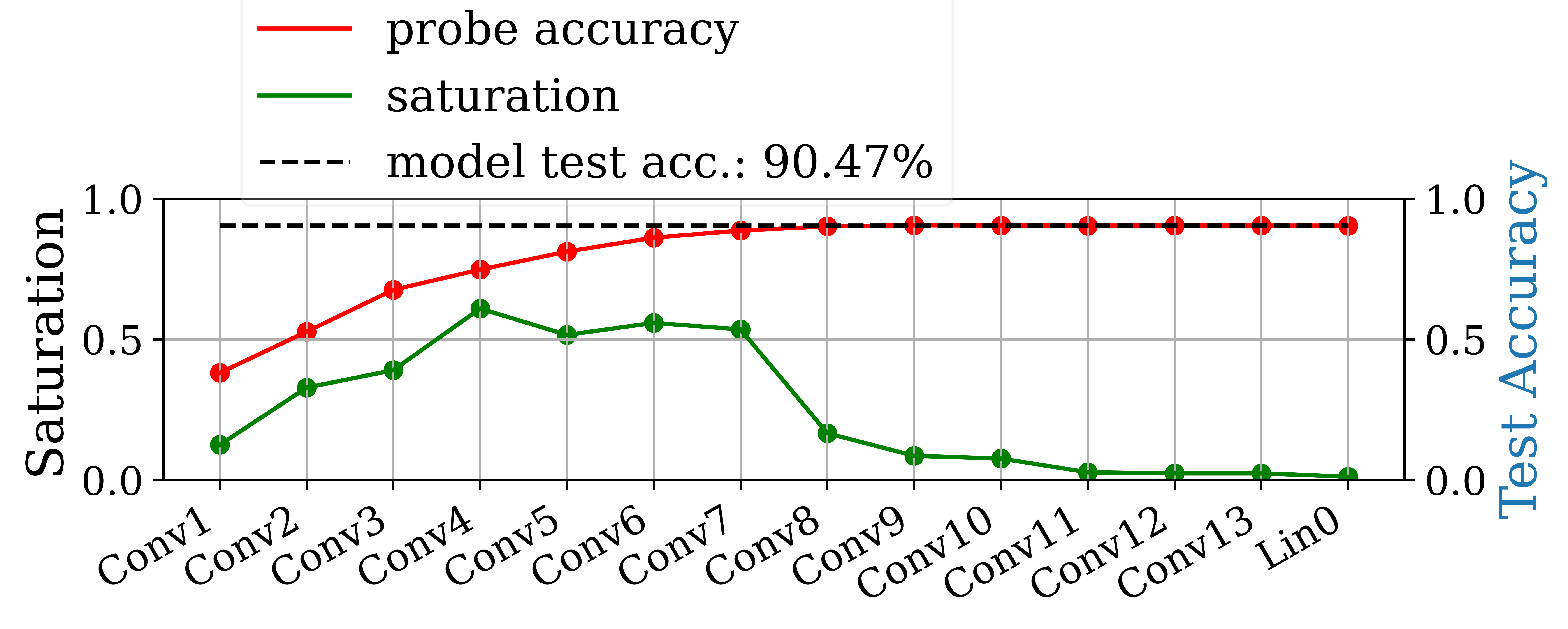
(a) $32\times 32$ without canvas

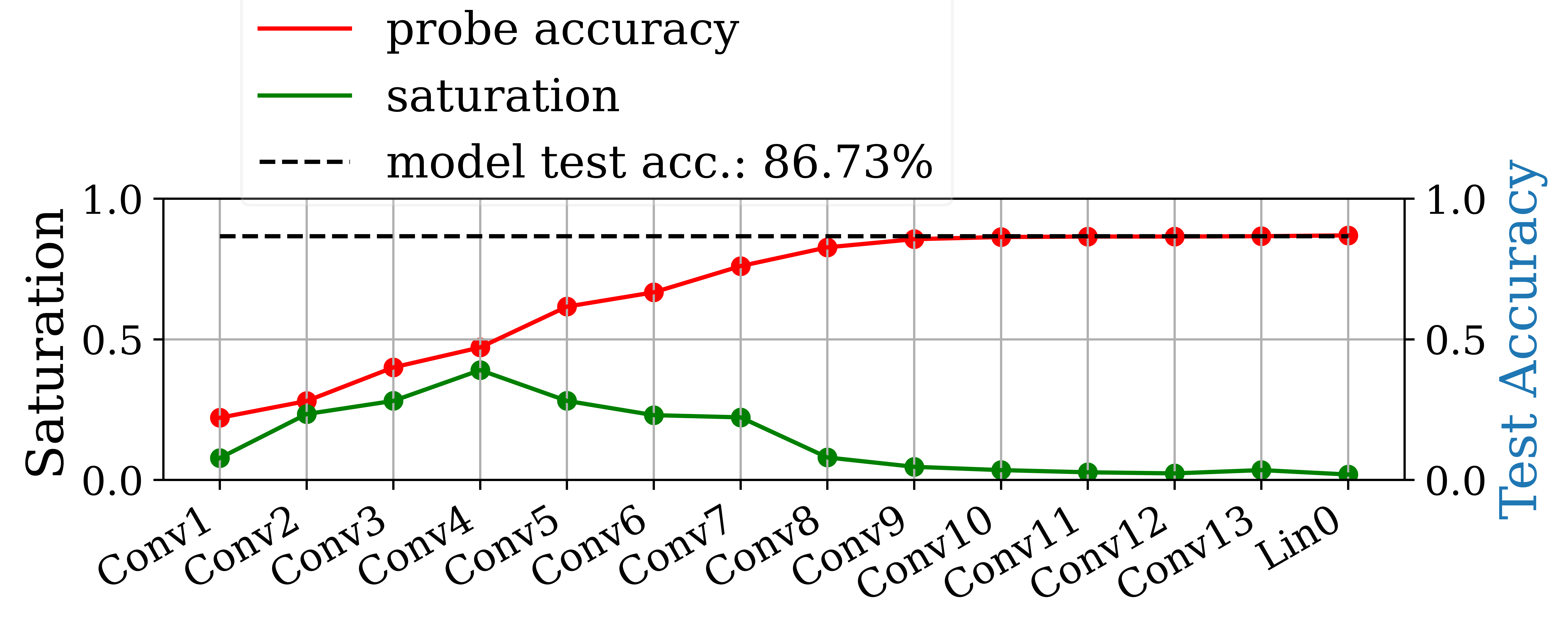
(b) $160\times 160$ with canvas

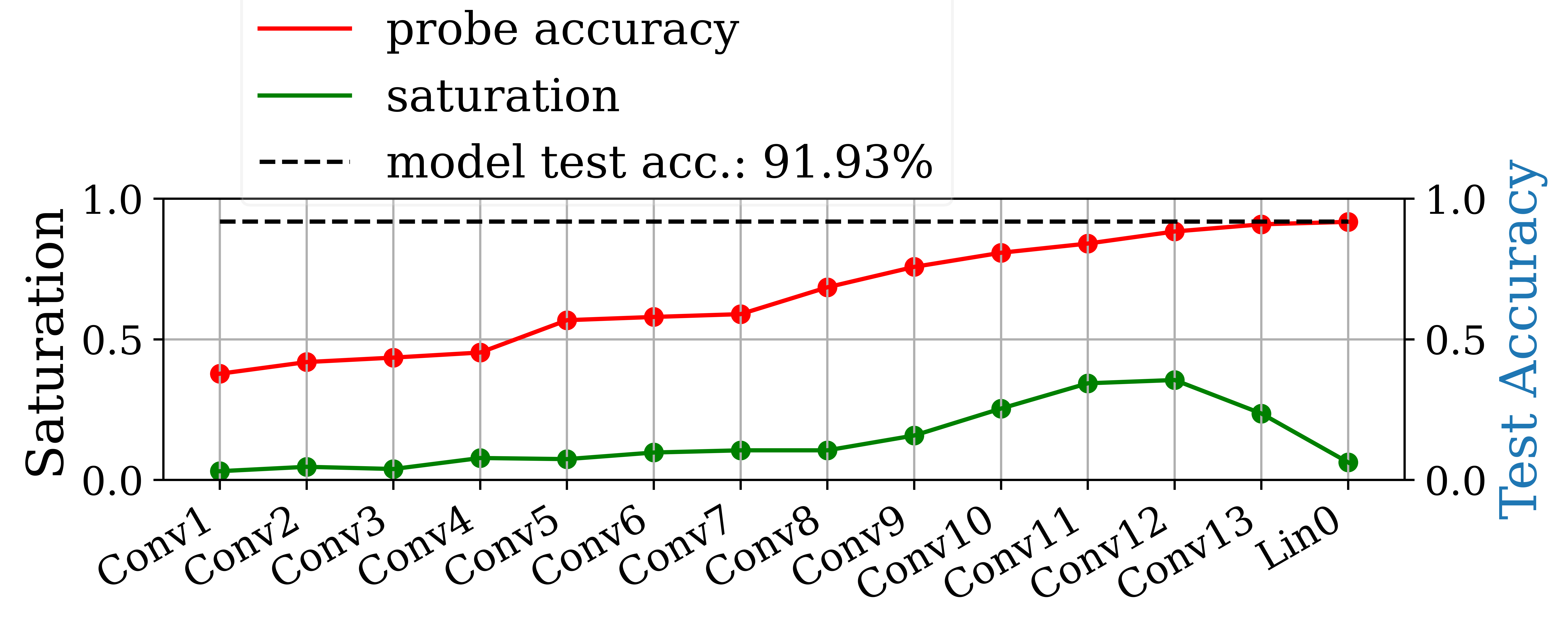
(c) $160\times 160$ upsampled

Figure 3: A tail of unproductive layers can be produced by placing the Cifar10 images on a $160\times 160$ pixel canvas. This indicates that locality of discriminatory features (essentially the size of the object) is responsible for the observed effect on the inference process.

To verify this experimentally we train models on a modified version of the Cifar10 dataset. In this version the Cifar10 images are randomly placed on a black canvas of $160\times 160$ pixels. This restricts the size of the object of interest and therefore all potentially discriminatory features to a square region of 32 pixels per side. If the absolute size of the object is influencing which parts of the network process the information, the resulting tail pattern and evolution of the probe performances should be similar to the same model trained on Cifar10 on its native resolution. The results in figure 3 show that this is the case. Saturation and probe performances behave very similar to training the model on $32\times 32$ pixels, while scaling the entire image to $160\times 160$ pixels distributes the inference process very differently (see figure 3c). The same effect can be reproduced with other models and datasets (see supplementary material).

We can conclude from this that the relevance of the input size when training classifiers comes from the size of the discriminatory features detected by the model. In other words, the size of the image is a heuristic for the size of the object of interest. This also means that the results depicted in this work are unlikely to generalize to tasks where objects of interest are more localized and varied like in most object detection datasets.

3.4 The role of the receptive field in relation to the object size

From the previous section we can derive that features of different sizes are recognized by different layers in the model. In this section we will investigate the causes of this phenomenon from an architectural point of view.

From the perspective of the architecture, the receptive field of a layer can be considered an upper bound for the size of recognizable features. Since the receptive field expands with every layer that has stride and/or kernel size greater than 1, increasingly larger features can be recognized. We hypothesize that for simple, sequential architectures like the VGG-family of networks , the receptive field is the dominating factor influencing presence and position of unproductive subsequences of layers.

(a) VGG11

(b) VGG13

(c) VGG16

(d) VGG19

Figure 4: The first convolutional layer processing input from a layer with a receptive field size greater than the input size can be seen as a border (marked with a black vertical line) between the ”solving” and the ”compressing” stage of the network. Only the highly saturated solving stage improves on the intermediate solutions as shown by the probes. The depicted models are from the VGG-family of networks by Simonyan & Zisserman (2014) and trained on Cifar10 with an input size of $32\times 32$ pixels.

We study this property of the receptive field by training the VGG-family of networks on Cifar10 and add the receptive field as an additional information to our analysis.

(a) ResNet18 (no res. connections)

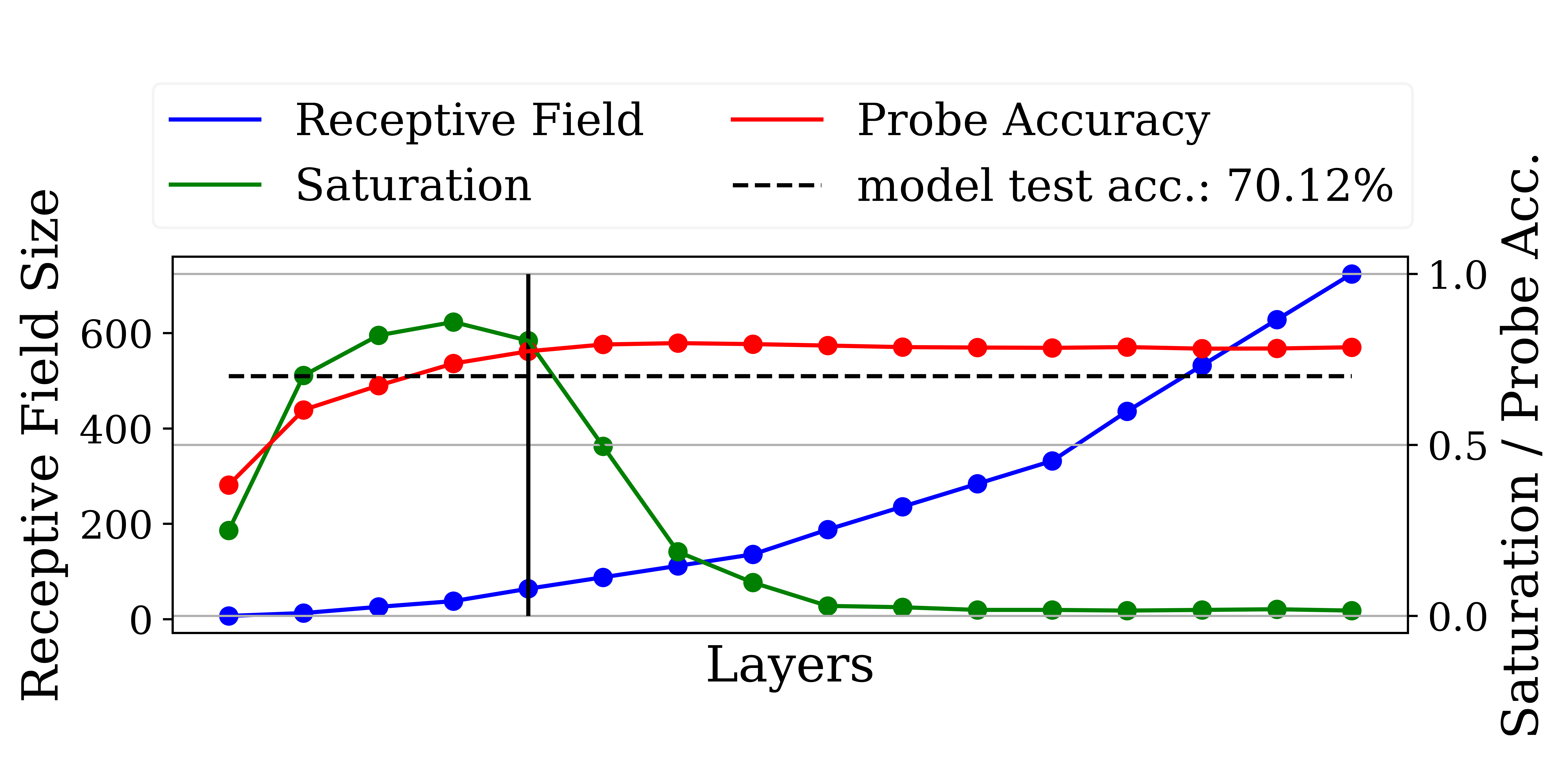
(b) VGG19 (dilation=3)

Figure 5: The behavior described in figure 4 translates to different sequential architectures as well. For instance ResNet18 with disabled residual connections uses mainly strided convolutional layers and has a significantly faster receptive field expansion due to the first two layers being downsampling layers. The VGG19 variant displayed here has the border layer shifted closer to the input compared to the original version displayed in figure 4, since the dilated convolutions increase the kernel size and therefore the expansion of the receptive field. All models are trained on Cifar10 with $32\times 32$ pixel input size.

In figure 4 we mark the first layer that processes input from a layer with a receptive field size greater than the input size with a black border. We will refer to this layer as the border layer. For all architectures, this border separates layers contributing to the inference process from layers that do not contribute to the quality of the inference significantly. This suggests that a layer in a simple, sequential architecture can only substantially improve the performance when novel information is integrated into positions on its feature map.

We investigate this observation further by testing architectures, which alter the receptive field size in different ways than the VGG-family of networks. We test the effect of dilated convolutions by training a modified VGG19 with a dilation rate of 2 in all convolutional layers. This modification effectively increases the kernel sizes of all layers, which in turn increases the receptive field size without changing the number of parameters. We also turn ResNet18 into a sequential model by removing the residual connections. The ResNet-family mainly uses strided convolutions for downsampling and also features more downsampling layers that are spaced differently compared to VGG-style models. This results in a much faster growth of the receptive field as well as a higher overall receptive field size.

From the results in figure 5 we can see that the behavior of both models is consistent with previous observations.

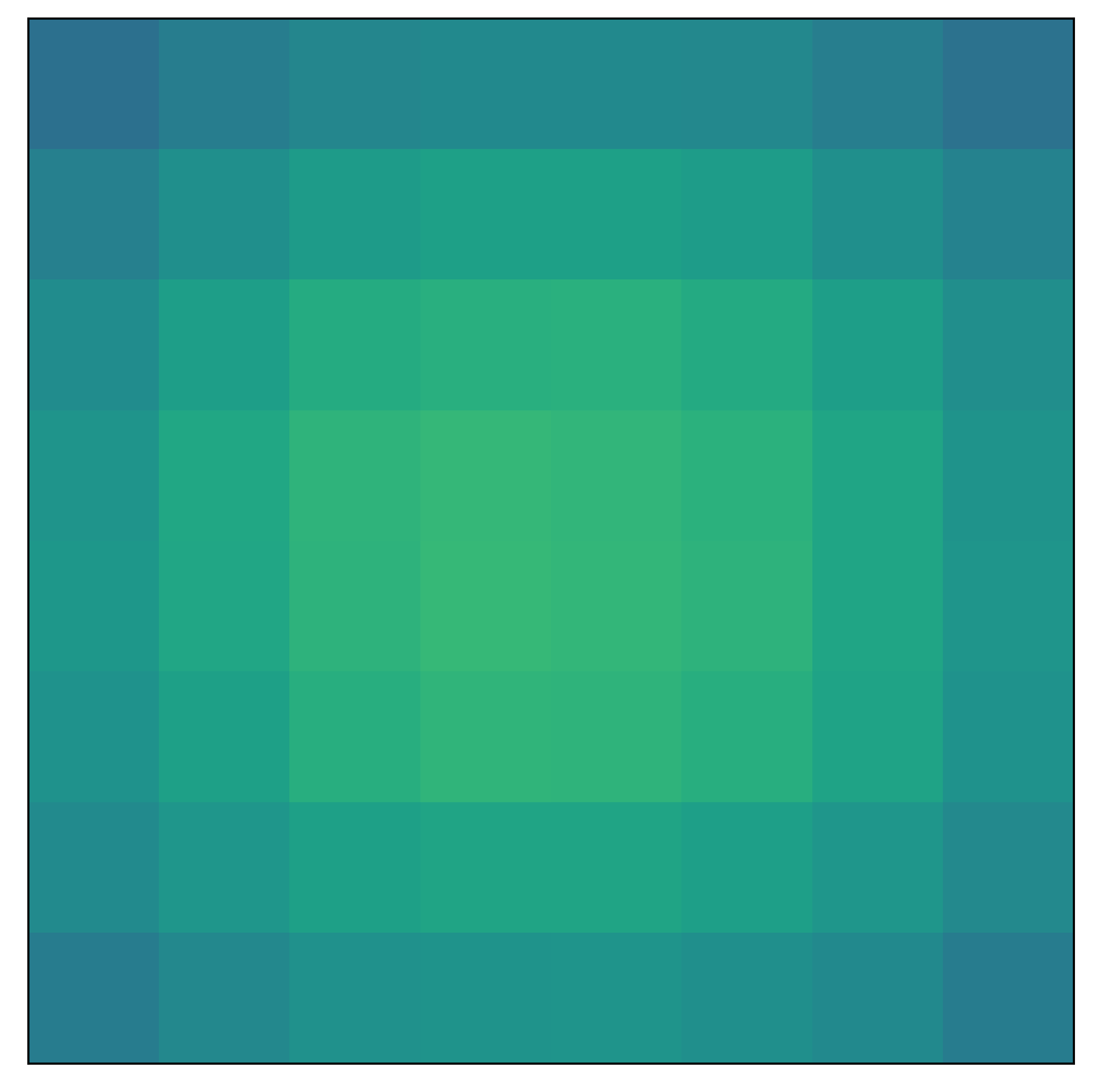
(a) Pre Border

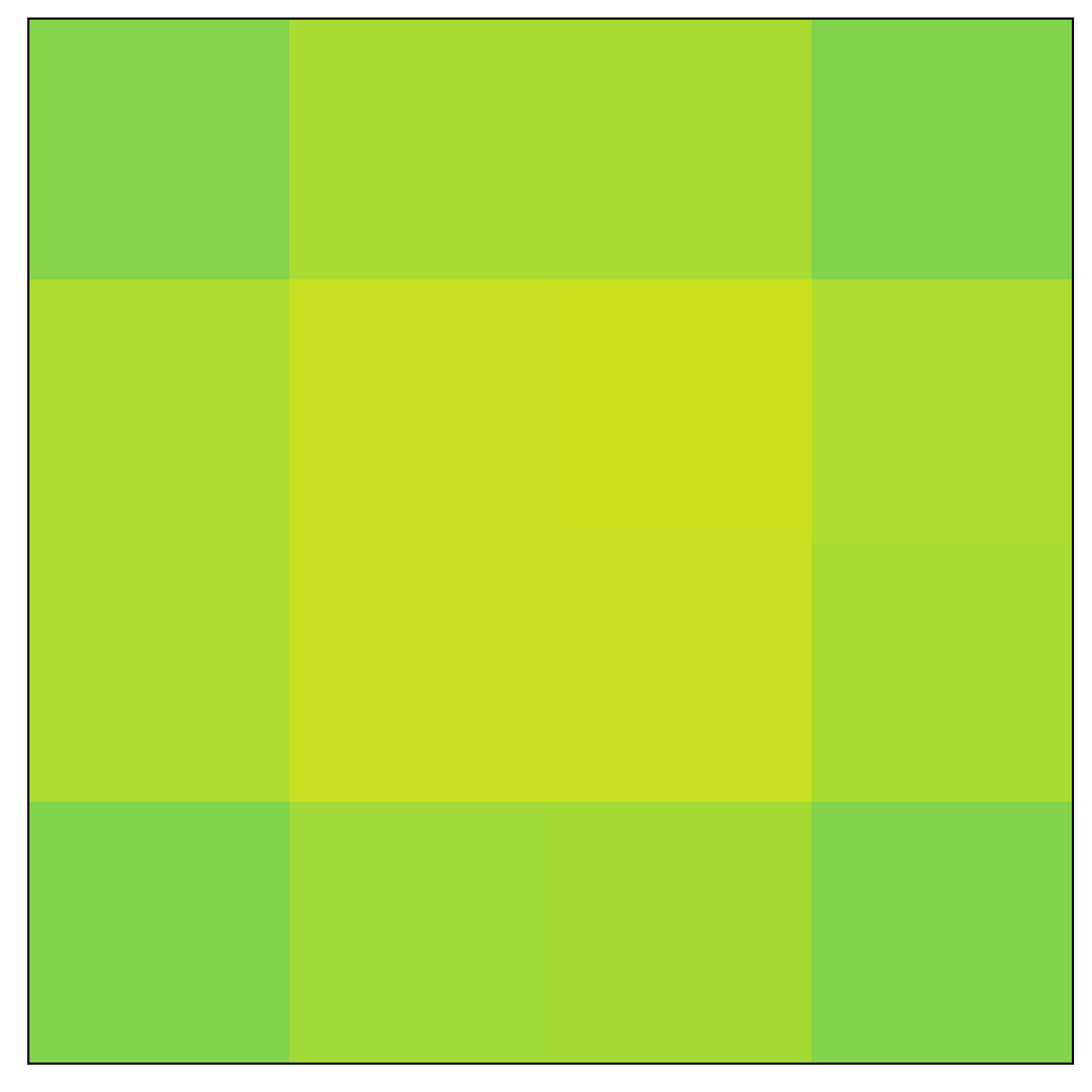
(b) Border

(c) Post Border

(d) Last Layer

(e)

Figure 6: The heatmaps display the relative performance of probes trained on individual positions of feature map to the performance of the model. The depicted model is VGG16 trained on Cifar10 and displayed also in figure 4. The depicted layers are the 5th, 8th, 9th and the last convolutional layer. We observe that the performance of probes on early layers is best in the center, where the receptive field can integrate the most information since the receptive field will not exceed the bounds of the image. This is still true for the border layer. However, all four inner positions of this feature map integrate information from the entire image and have reached the performance of the softmax output of the model as a result. The last two depicted layers visualize the activity in the low saturated tail. As the receptive field expands more positions on the feature map encode information from the entire image and achieve similar probe performances. This homogenisation of partial solutions results in a decreasing number of high variance eigendirections which in turn results in low saturation. This explains the low saturated tail of layers seen on networks trained on too low resolution.

Finally, we investigate how the solution develops inside the feature maps of different parts of the network. We modify our method of logistic regression probes by applying a single probe to every position of every layer’s feature map. We then compute the relative performance of the probes by dividing the probe accuracy with the network‘s accuracy (both evaluated on the test set). By doing so we can visualize the quality of the partial solutions contained in every position of the feature map based on their position. We observe in figure 6 that the central positions on the feature map generally perform best in early layers, while outer positions perform increasingly worse, with the corner positions generally being the worst. We suspect that the receptive field is at least partially responsible for this, since outer positions on the feature map will receive more black padding and thus less information with the receptive field expansion as a center pixel.

Another interesting observation in figure 6 is that the center most positions on the feature map contain partial solutions roughly equivalent to the performance of the entire model. As the saturation drops and layers become part of the low saturated tail, the partial solution quality becomes increasingly homogeneous across feature map positions. In the last layer each vector on the feature map is as linearly separable with regards to the classification task as the average pooled solution. We conclude based on these measurements that this homogenisation of partial solution quality is also responsible for the drop in saturation.

Based on these observations we can conclude that simple, sequential neural networks may develop two stages of inference when the image is smaller than the receptive field size of the model: The first being the solving stafe, where the data is processed incrementally to achieve loss minimization. The second stage, starting from the border layer, is the compressing stage. This stage compresses the latent space by homogenisation of the partial solutions for every position in the feature map.

3.5 The role of residual connections

Residual connections are a popular component used in many neural architectures (He et al., 2015; Iandola et al., 2014; Szegedy et al., 2016; Tan & Le, 2019). According to He et al. (2015) the networks with residual connections are able to add ”deltas” to the existing representation of the data rather than transforming it entirely. The residual connection itself does not expand or change the receptive field. After the residual connection is added to the output of a convolutional layer, information based on multiple receptive field sizes is present in the feature map. This allows features based on lower receptive field sizes to ”skip” layers and to be processed later in the network, resulting in the network being able to distribute the inference on more layers.

The aforementioned claims about the effects of residual connections suggest, that models utilizing residual connections are able to utilize layers for improving the prediction after the border layer. The border layer is the first layer to receive an input produced by a layer with a receptive field size larger than the image. In sequential architectures it is also the layer separating the solving and compressing stage of the model.

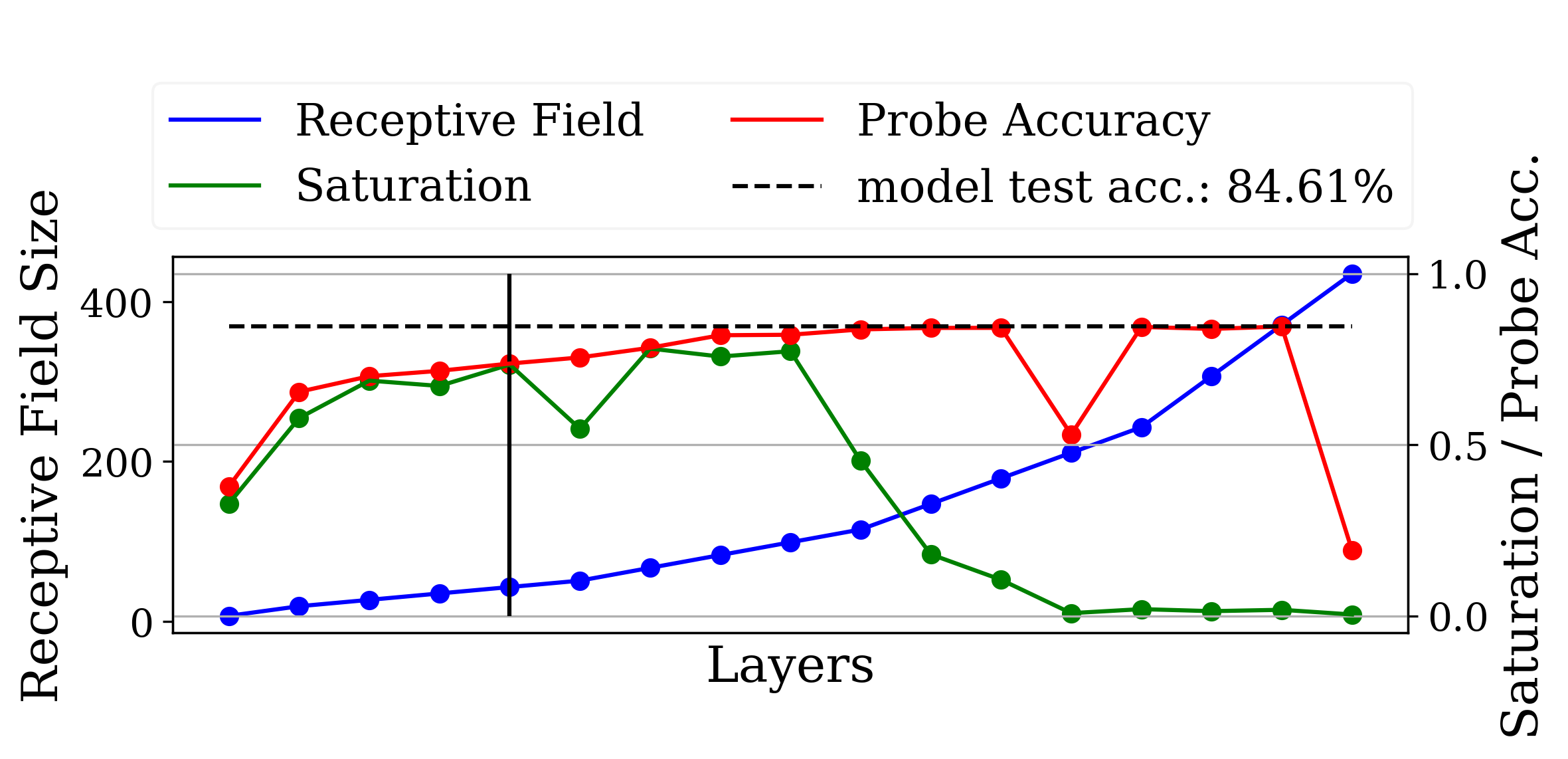
(a) ResNet18

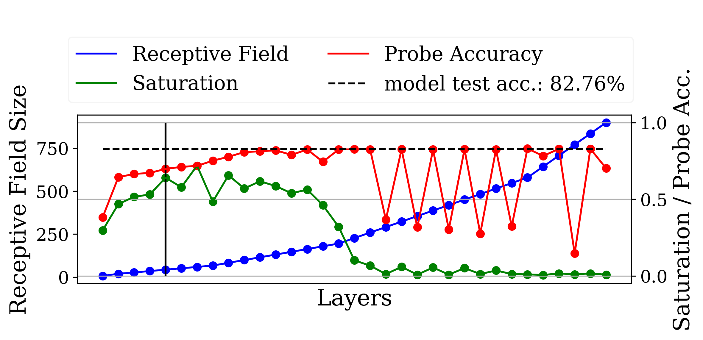
(b) ResNet34

Figure 7: Residual connections allow networks to utilize layers past the border layer (marked with the horizontal bar). The zick-zack-pattern and drops of probe performances observed in both networks are artifacts previously observed by Richter et al. (2020) and Alain & Bengio (2016). These indicate that the networks attempt to ”skip” the convolutional layers in the low saturated tail. It is also worth noting that these skips are only present on later layers which are part of the tail.

We can confirm this by looking at the results in figure 7. Both networks improve the probe performances and stay highly saturated long after the border layer has processed the data. We can attribute this behavior to the residual connections, since we tested ResNet18 without them in the previous section (see figure 5), resulting in behavior consistent with other sequential architectures (and lower performance).

While the presence of residual connections has a positive effect on the predictive performance of ResNet18 (84.61% accuracy with and 79.05% accuracy without residual connections), the performance still remains worse than VGG-style models. We attribute this to lower overall receptive field size of VGG19, which is only 252 pixels. ResNet models downsample more aggressively in the beginning, resulting in receptive field sizes of 413 (ResNet18) and over 800 pixels (Resnet34) respectively. This suggests that matching the receptive field size with the input size remains important when using residual connections in the architecture.

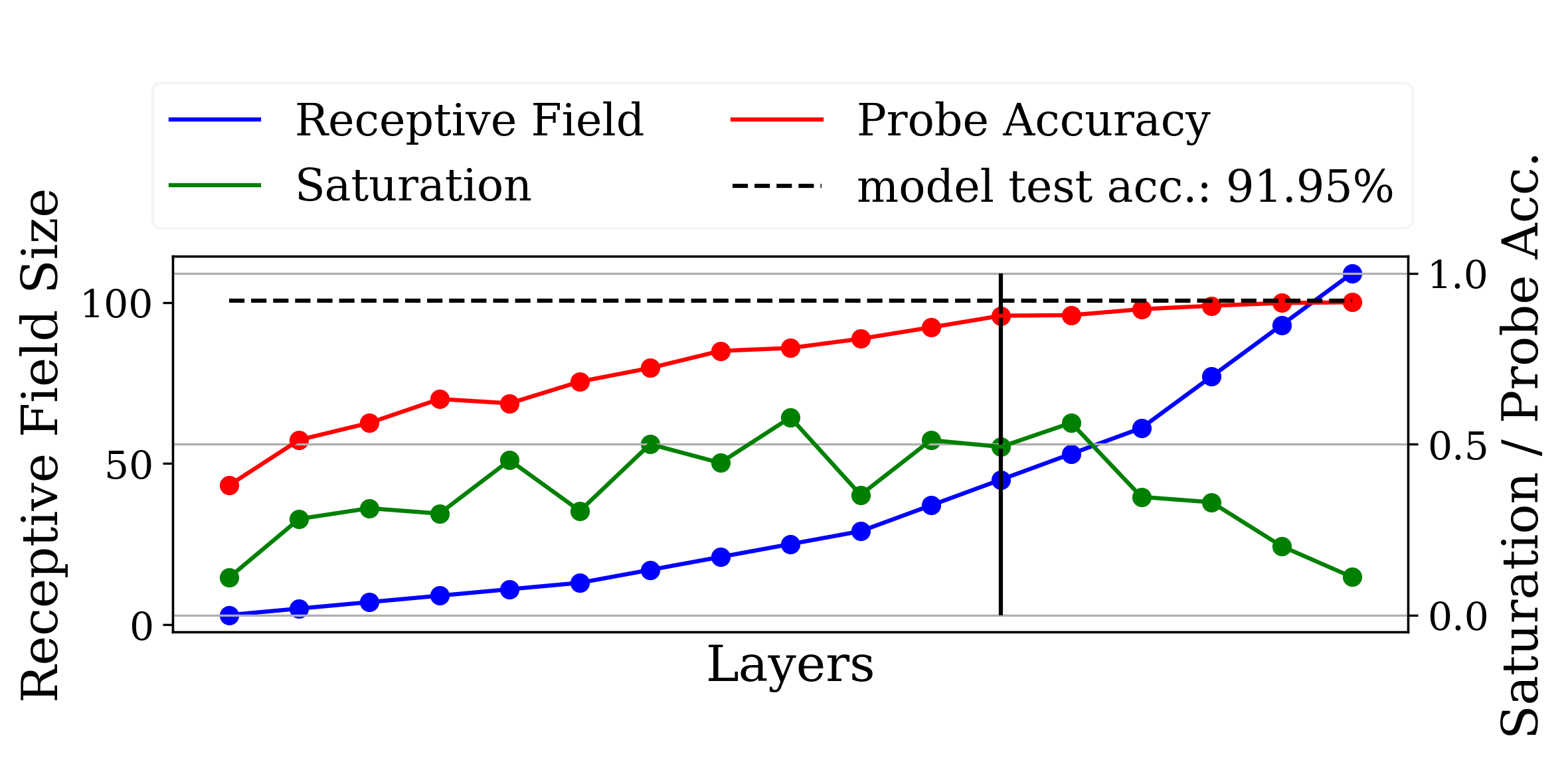
(a) Cifar10 optimized ResNet18

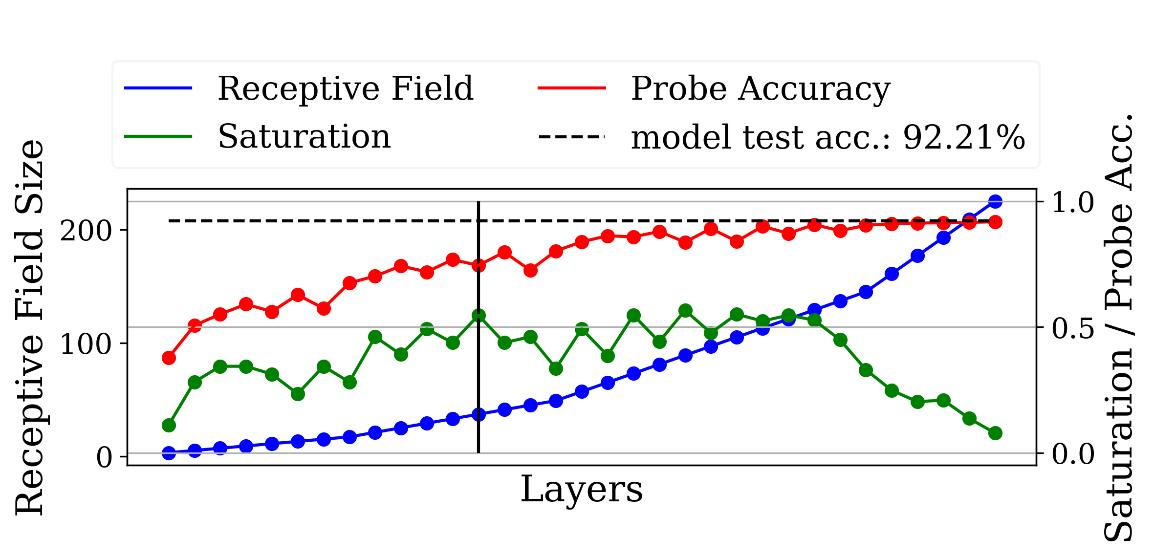
(b) Cifar10 optimized ResNet34

Figure 8: Cifar10 optimized version ResNet18 and 34 have a roughly quartered receptive field size in every layer. These networks still display similar behavior as the ImageNet optimized version when it comes to the border layer. However, the reduction in the receptive field size has further removed the low saturated tail and lead in both cases to a steady increase in performance over the entire networks structure.

Therefore it should be possible to improve the performance of the (ImageNet optimized) ResNet18 and 34 by reducing the size of the receptive field. This was implicitly done by He et al. (2015), who proposed additionally to the ImageNet optimized versions of ResNet a Cifar10 optimized variant. The Cifar10 variant of ResNet has no max-pooling layer and the first layer has its stride size in kernel size halved. By doing so the receptive field of ResNet18 for example was reduced from 413 (ImageNet optimized) to 109 pixels (Cifar10 optimized). The effect of these reductions can be seen in figure 8: the proportion of low saturated layers is drastically reduced for both models and the inference process is now well/more evenly distributed. Thus the performance increases in both cases compared to the ImageNet optimized models. The accuracy of ResNet18 improves from 84.61% (ImageNet optimized) to 91.95% (Cifar10 optimized) ResNet34 improves from 82.76% to 92.21%. This example illustrates that a mismatch of dataset and architecture can be resolved by altering the architecture in a way that brings the receptive field size closer to the input resolution.

4 Conclusion

For the longest time in deep learning, developing increasingly bigger and more complex models to improve performance has been the norm. Our work provides a counterpoint, showing that the neural architecture and the visual properties of the dataset must match in order to avoid inefficiencies like layers not contributing to the quality of the solution and sub-optimal predictive performance. We show that the receptive field size is a primary architectural factor in this interaction. We further show that the residual connections can counteract (but not entirely mitigate) mismatches of input size and receptive field size by allowing more layers to contribute to the inference qualitatively. Finally, we demonstrate that probe classifiers and saturation are useful tools to analyze the relationship between dataset and model architecture allowing the optimization of CNN design in a principled way. We conclude that the size of the input image matters for optimal predictive and computational performance.

Appendix A Code and Experimental Setup

The full code used for conducting all depicted experiments as well as a guide for reproducing the results can be found here:

https://anonymous.4open.science/r/d04fa611-aa00-4c22-9158-5af363b68c3a/

Appendix B Handling convolutional feature maps when computing probe performance

A practical problem for computing the performance of probes is the size of convolutional feature maps. In order to make the experiments computationally tractable, it is necessary to reduce the dimensionality of those feature maps.

When probes were first proposed by Alain & Bengio (2016) two ways of handling this practical problem are tested, Global Average Pooling (GAP) and randomized subsampling of the feature maps. However, random sub sampling introduces artefacts (Richter et al., 2020). Also, Richter et al. (2020) conducted GAP experiments by looking on the ablative effects of downsampling and adaptive pooling strategies on VGG and ResNet model trained on input sizes between $32\times 32$ pixel $224\times 224$ pixel on Food101 and Cifar10 (Bossard et al., 2014; Krizhevsky et al., 2010). We conclude that the effect on Global Pooling are diminishing as the feature map increases but the overall structure does not change. In order to reduce this ablative effect while still making probe performance computation practical as much as possible we decided on a $4\times 4$ adaptive average pooling over the feature maps. The experiments showed diminishingly small changes in the features and the overall performance levels of probes compared to larger downsampling strategies.

In experiments for showing the evolution of the of the feature map in conjunction with the receptive field expansion, we also trained probes on each position of all feature maps, which allows us to generate performance heat maps, where we are able to show how much information required for solving the task is contained on a specific position of the feature map.

B.1 A more detailed explanation on receptive field size and its computation

The receptive field size is a property of a layer inside a neural network architecture. It describes the size (height and width) of an rectangle on an infinitely large input image. This area contains all pixels that can influence the output of a single position of the convolutional kernel on the feature map. Simply speaking, it describes the spatial limits of visual features detectable by the respective layer.

It is worth noting that the size (in theory) is a rectangle, since the kernels of CNNs may have an arbitrary height and width. therefore the receptive field size is technically a 2-tuple consisting of two integers describing height and width of the rectangle. However, conventionally networks have square kernels and are fed square images, which are either padded, cropped or scaled to the correct aspect ratio using data augmentation (Krizhevsky et al., 2012; Simonyan & Zisserman, 2014; He et al., 2015; Szegedy et al., 2015, 2016; Tan & Le, 2019; Iandola et al., 2016, 2014). We thus refer to the receptive field size as an integer for the sake of simplicity.

B.1.1 Computing the receptive field

For convolutional neural networks with a sequential structure (no multiple pathways during the forward pass) the receptive field size can be computed analytically. We refer to the receptive field $r$ of the $l$th layer of sequential network structure as $r_{l}$ (with $r_{0}=1$, which is the ”receptive field” of the input). For all layers $l>0$ in the convolutional part of the network the receptive field can be computed with the following formula:

$$r_{l}=r_{l-1}+((k_{l}-2)\prod^{l-1}_{i=0}s_{i})$$ (2)

Where $r_{l-1}$ is the receptive field of the previous layer, $k_{l}$ refers to the kernel size of layer $l$ (with potential dilation already accounted for) and $s_{i}$ the stride size of layer $i$. In the simplest case, which is the first convolutional layer of the neural architecture $r_{1}$ and stride size of 1, the receptive field is exactly the size of the kernel, therefore the receptive field size is the kernel size. When convolutional layers are stacked, the receptive field for every layer $l$ with a kernel size $k_{l}\neq 1$ expands the receptive field for following layers, because the filter integrates information of an area of the input feature map into a single output position. Downsampling and pooling layers that reduce the size of the feature map will have $s_{i}\neq 1$, which has a multiplicative effect on the receptive field expansion of consecutive layers. In simple cases like VGG16, where the max-pooling layers are $2\times 2$ filters with $s_{i}=2$, this can be intuitively imagined as 4 adjacent pixels being summarized into a single ”super pixel”. This effect on the growth of $r$ is also compounding exponentially when multiple downsampling layers are employed in the neural architecture, which is generally the case for most popular architectures (Simonyan & Zisserman, 2014; He et al., 2015; Szegedy et al., 2015, 2016; Iandola et al., 2014, 2016; Zhang et al., 2017; Tan & Le, 2019; Szegedy et al., 2016; Iandola et al., 2016).

B.1.2 The receptive field in network with multiple pathways

The method described previously allows the computation of the receptive field for sequential architectures with each layer having at most a single previous layer. However, since the advent of deep learning multiple pathways have been common in neural architectures. In this scenario there $s_{i}$ and $r_{l-1}$ may be tuples of values with each element describing the stride size and the receptive field size of a pathway. However, the common strategies for funneling multiple paths into a single successive layer are simple element-wise operation (like additions and multiplications) or concatenations of the respective stacks of feature maps produced by each path. Both cases have in common that the size of the feature maps must agree, which is achieved by either different means influencing the size of the receptive field. However, we are not interested in knowing exactly which feature map in an output layer considers which information. We are only interested in the size of the area that contains all information that can theoretically influence a position in the feature map. Hence, we ignore all pathways except the one with the largest receptive field. It is worth noting that we make the assumption that all pathways downsample the image identically $s_{l,1}=s_{l,2}=...=s_{l,n}$, so that the growth rate of the receptive field is increased evenly on different pathways. While this assumption is not true for all possible architectures it holds true for all architectures considered in this paper and most popular architectures like VGG, ResNet, InceptionV3 and EfficentNet (Simonyan & Zisserman, 2014; He et al., 2015; Szegedy et al., 2016; Tan & Le, 2019).

Appendix C Resolution Shifts the Distribution of the Inference Process on different Models

In Section 3.2 we show on a ResNet18 architecture how resolution affects the distribution of the inference process by training ResNet18 on 3 different resolutions on Cifar10.

To show that this observation does generalize we repeat the experiment. We use TinyImageNet as a more complex but still small resolution problem. We further show that the hypothesis holds also true for VGG16 and ResNet50 models.

C.1 VGG16 - Cifar10

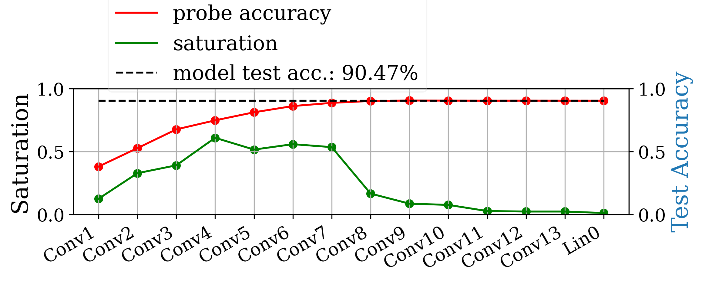
(a) $32\times 32$ (Cifar10 native resolution)

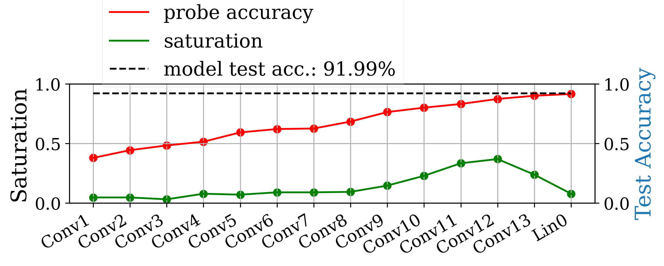
(b) $160\times 160$

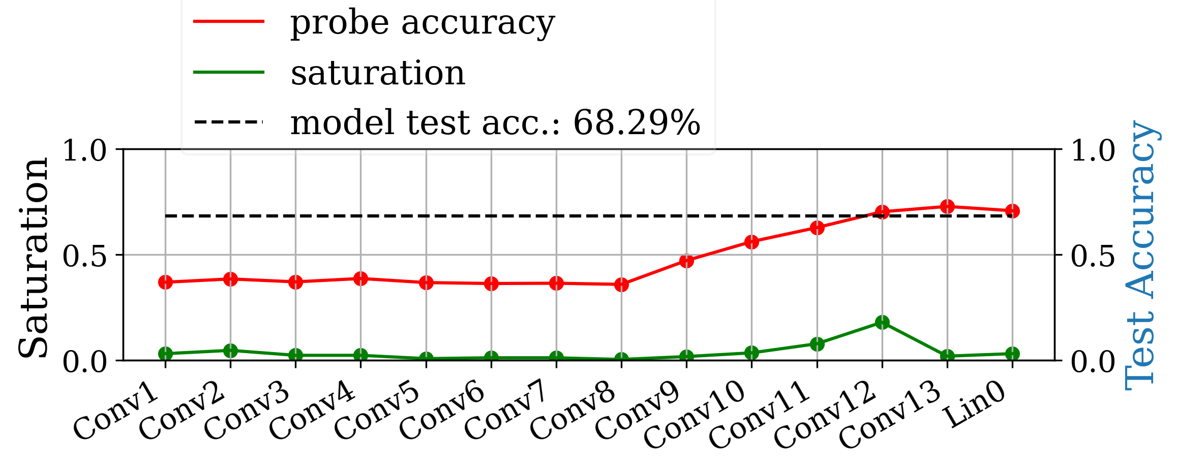
(c) $1024\times 1024$

Figure 9: Reproduction of the experiment depicted in figure 2 using the VGG16 architecture. Because of the larger memory footprint of the model, the batch size of this experiment is reduced to 20. The observed pattern stays the same. Low resolution results in a tail close to the output, while high resolution exhibits a tail at the input.

The (medium sized) resolution of $160\times 160$ pixels performs best.

C.2 ResNet18 - TinyImageNet

TinyImageNet consists of 200 classes of $64\times 64$ images. Therefore the first experiment is conducted on $64\times 64$ pixel input resolution instead of $32\times 32$ pixel resolution, since this is the basic resolution of the dataset.

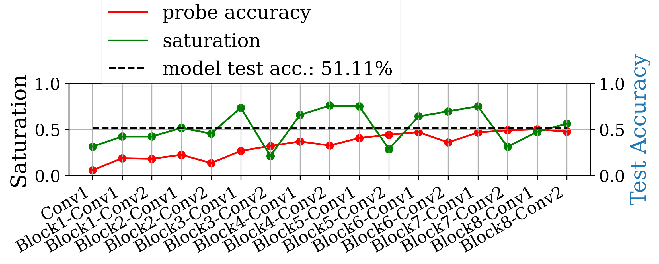
(a) $64\times 64$ (TinyImageNet native resolution)

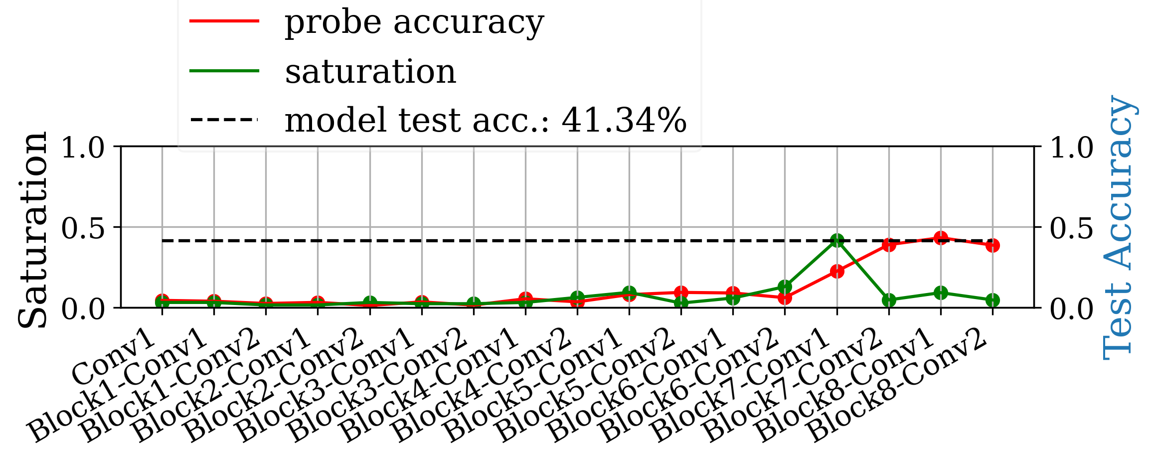
(b) $1024\times 1024$

Figure 10: The higher native resolution combined with the residual connection removes the tail pattern even at $64\times 64$ pixels for ResNet18. We see that a tail pattern can be produced in the input part of the network when the resolution is increased drastically to $1024\times 1024$, confirming observations from Cifar10.

C.3 ResNet50 - Cifar10

Due to an error in the setup, the mid-sized image experiment was conducted with a $160\times 160$ pixel resolution instead of $224\times 224$. However, even thought the resolution was altered it still shows the exspected behavior observed with other models.

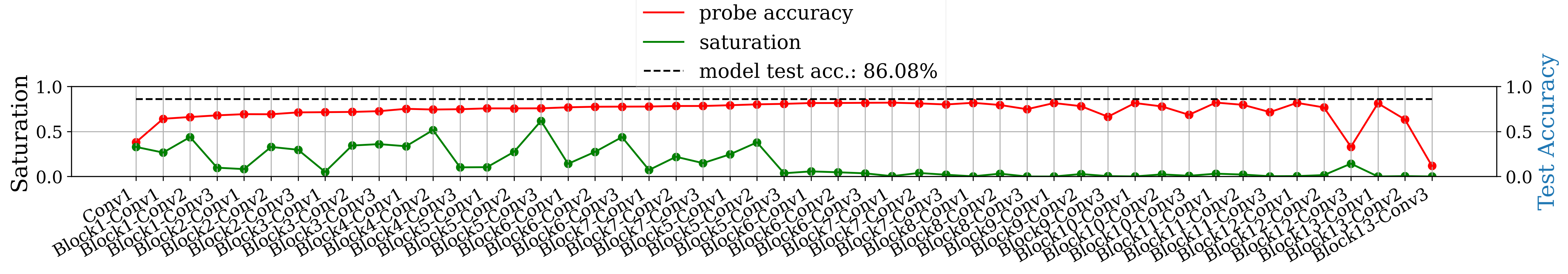
(a) $32\times 32$ (Cifar10 native resolution)

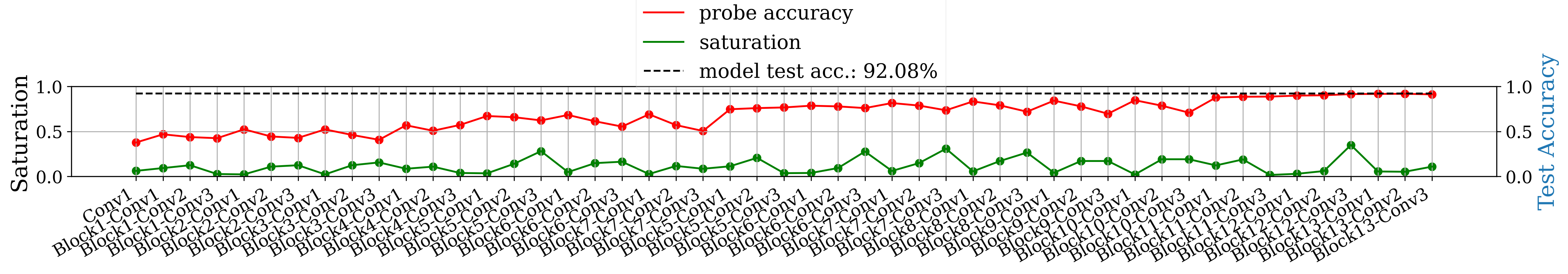
(b) $160\times 160$ (ResNet standard)

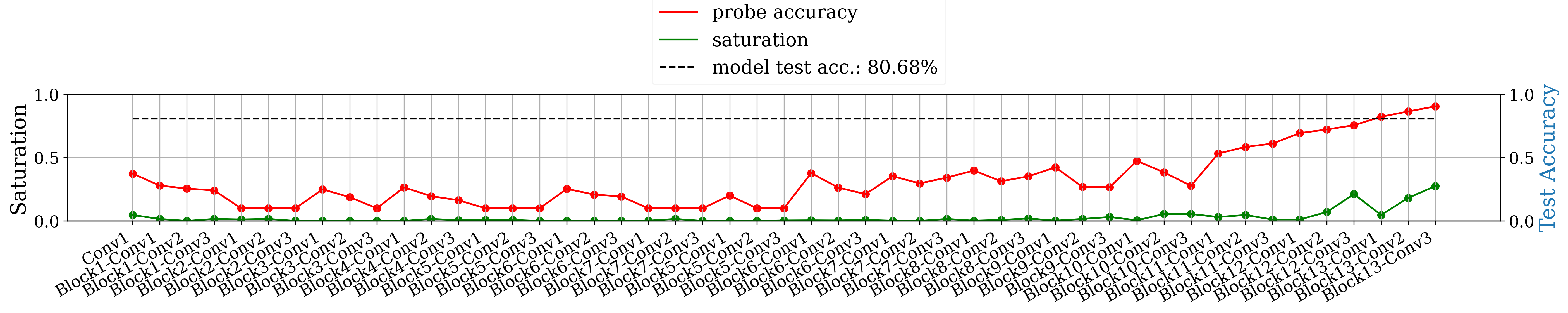
(c) $1024\times 1024$

Figure 11: Producing a tail pattern in the near the input and the output is also possible for very deep models like ResNet50 with the exspected effects on the performance. The Bottleneck-Modules with $1\times 1$ convolutions and varying filter sizes induce additional noise into saturation patterns.

Appendix D Object Size Experiments on MNIST and ResNet models

In Section 3.3 we make the claim that the observed relation of input resolution and the performance of the model is an artifact caused by the underlying interaction of object size and neural architecture. We repeat the experiments that demonstrate this claim on ResNet-style models as well as on the MNIST dataset. As we can see in figure 12 and figure 13 and figure 14, the results are consistent with the observations shown in the paper in all three scenarios.

D.1 ResNet18 - Cifar10

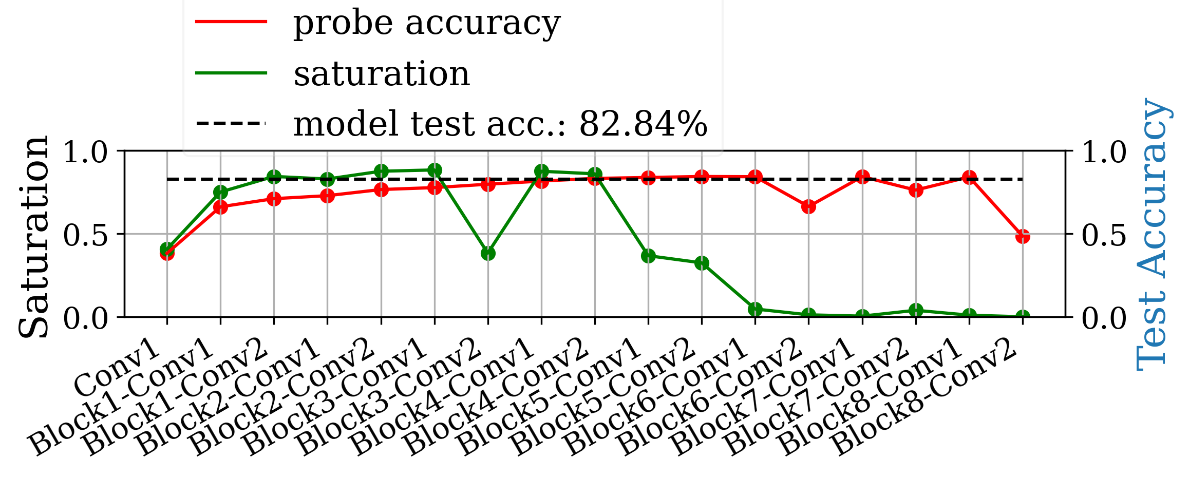
(a) $32\times 32$ without canvas

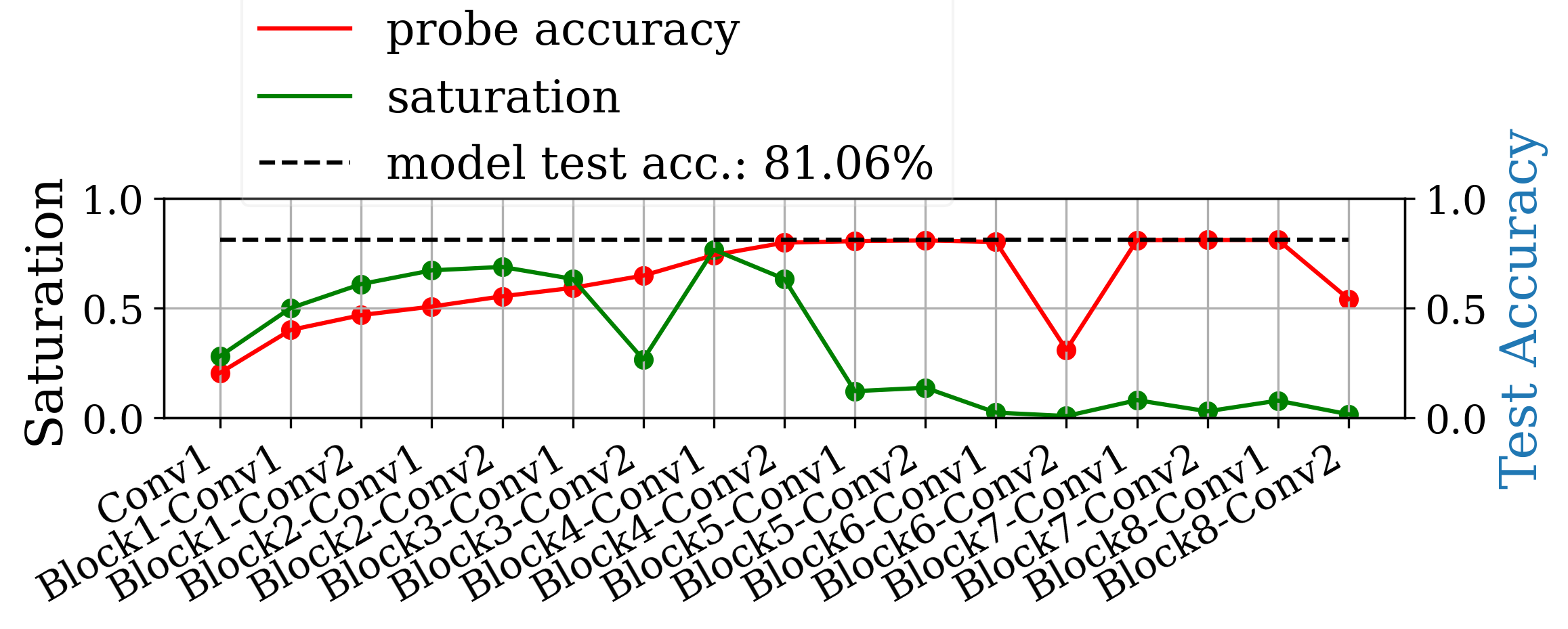
(b) $160\times 160$ with canvas

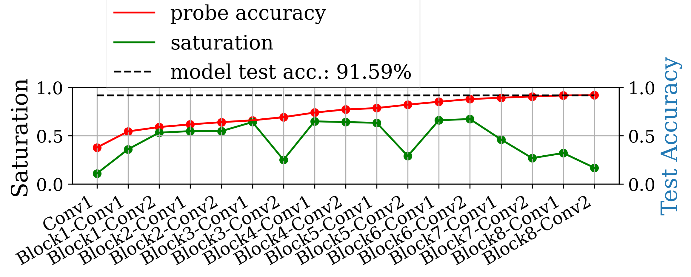
(c) $160\times 160$ upsampled

Figure 12: Random Positioning Experiments conducted with ResNet18 on Cifar10 data.

D.2 VGG16 - MNIST

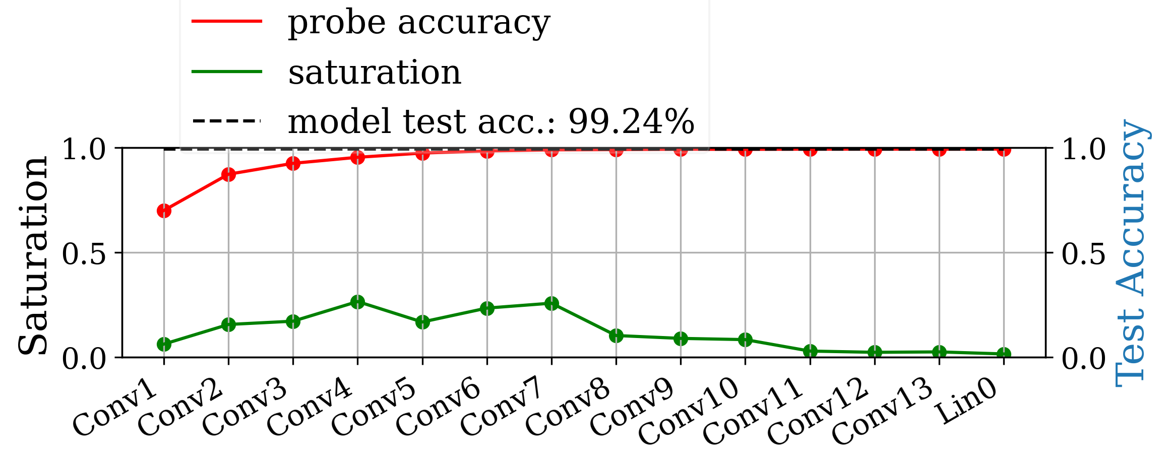
(a) $32\times 32$ without canvas

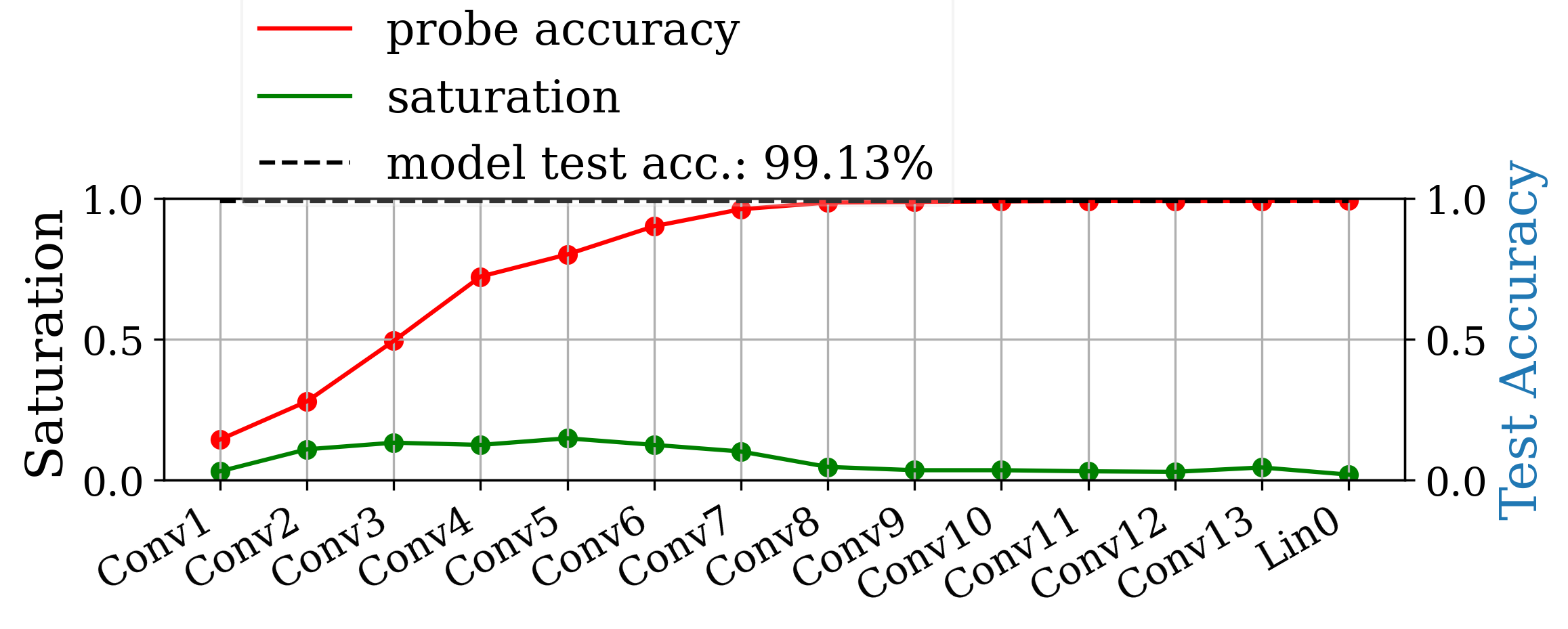
(b) $160\times 160$ with canvas

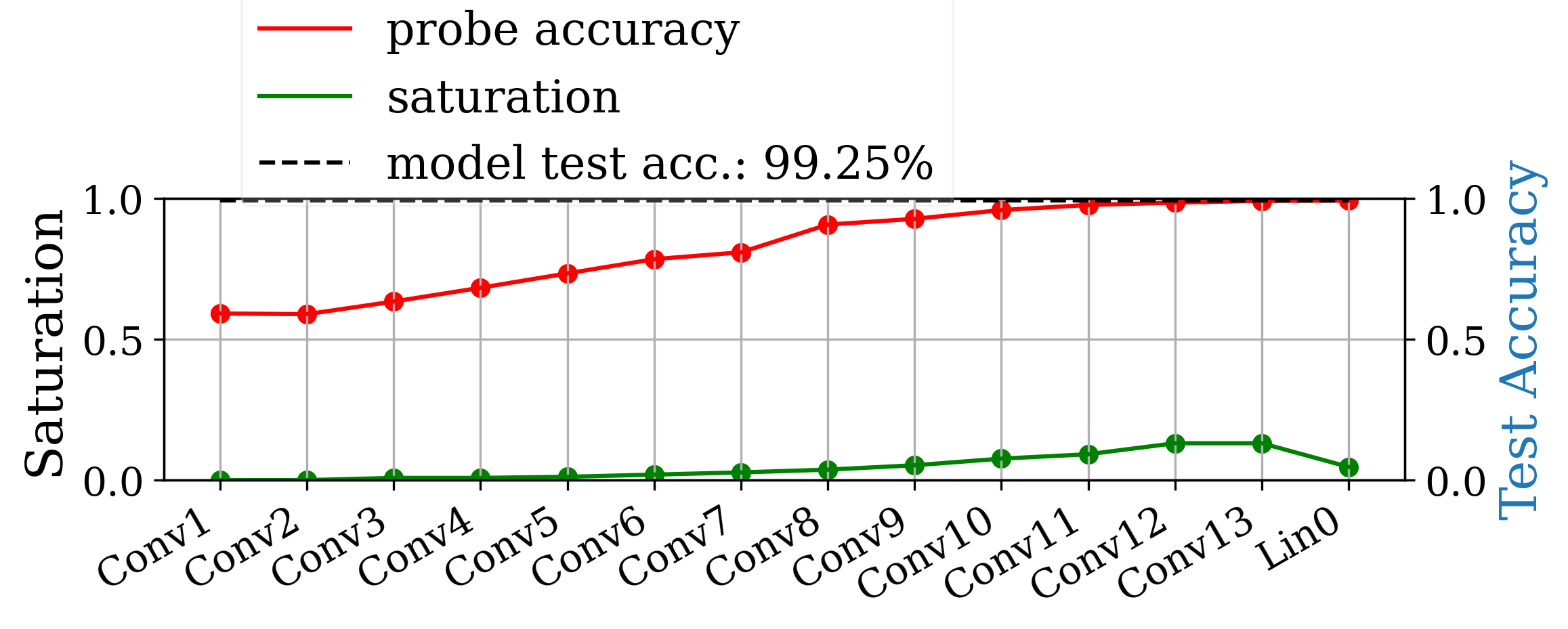
(c) $160\times 160$ upsampled

Figure 13: Random Positioning Experiments conducted with VGG16 on MNIST data.

D.3 ResNet50 - Cifar10

(a) $32\times 32$ (Cifar10 native resolution)

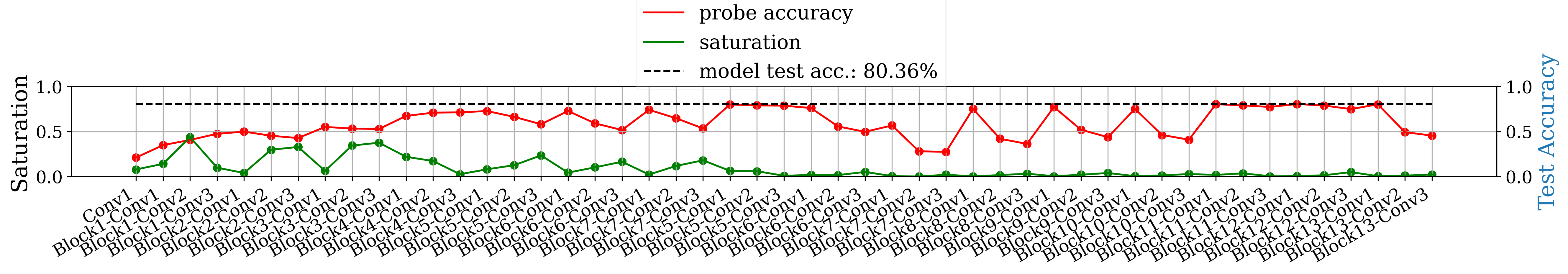
(b) $160\times 160$ with canvas

(c) $160\times 160$ upsampled

Figure 14: Random Positioning Experiments repeated on ResNet50.

Appendix E Additional Experiments Regarding the Relationship of Receptive Field and Input Resolution

The following experiments show additional observations made regarding the role of the receptive field size. When we training the models on the (arguably more difficult) TinyImageNet dataset using the same setup, the behavior stays consistent with our previous observations (see figure 15). However, if the problem is easy to solve it is possible for the model to mostly saturate probe performance before the saturation ”tail” starts. We can see an example of this in figure 16. When looking closely we can still see very slight improvements made until the border layers is reached. However, the improvements are hard to observe, which is also the reason why we only show MNIST results in the supplementary material.

We also observe that skip-connections have a statistically significant performance impact and that different combinations of residual connections distribute the inference process differently. To test this, we disabled different combinations of residual connections in ResNet18 while training Cifar10.

E.1 TinyImageNet Results

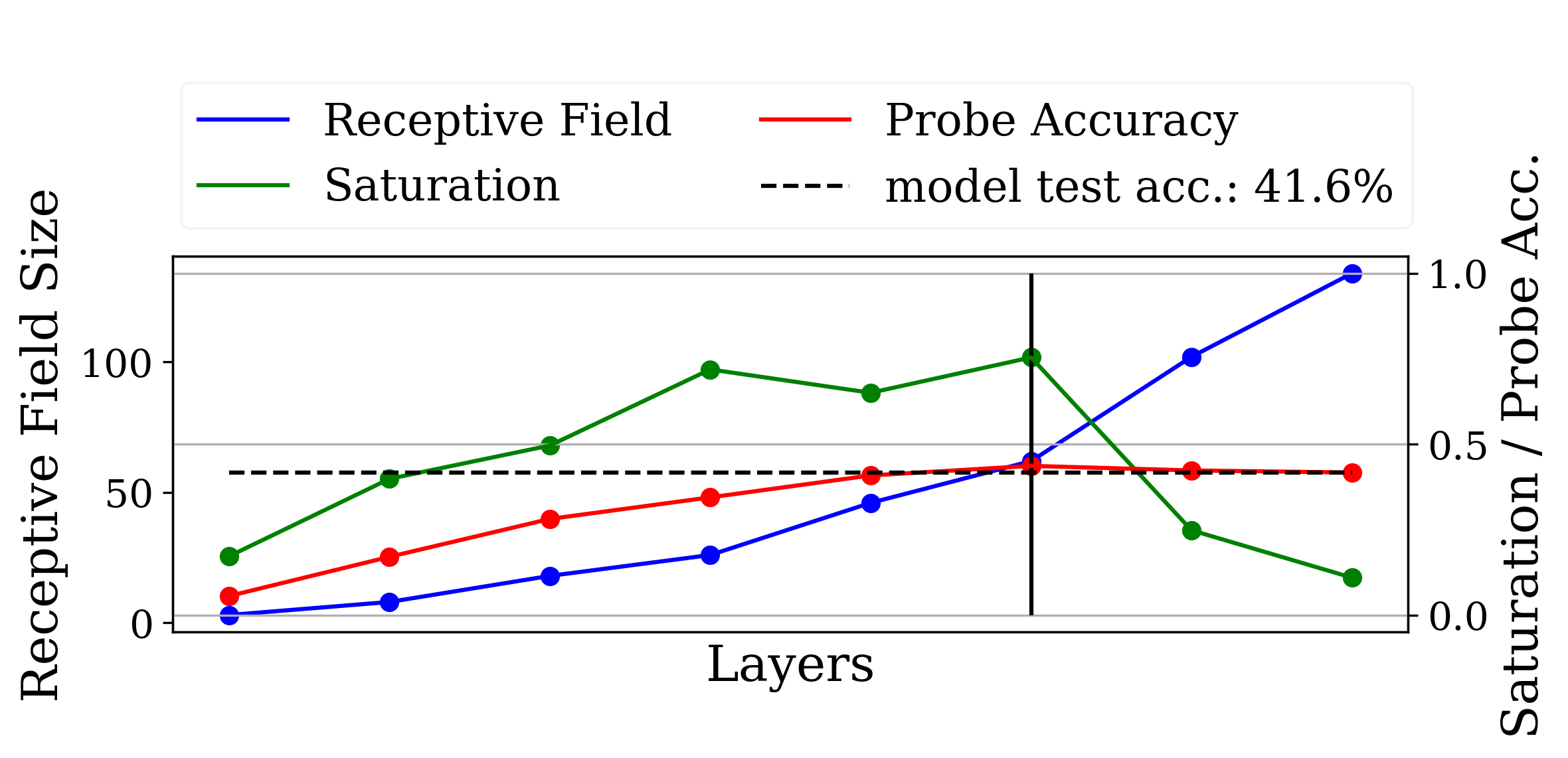
(a) VGG11

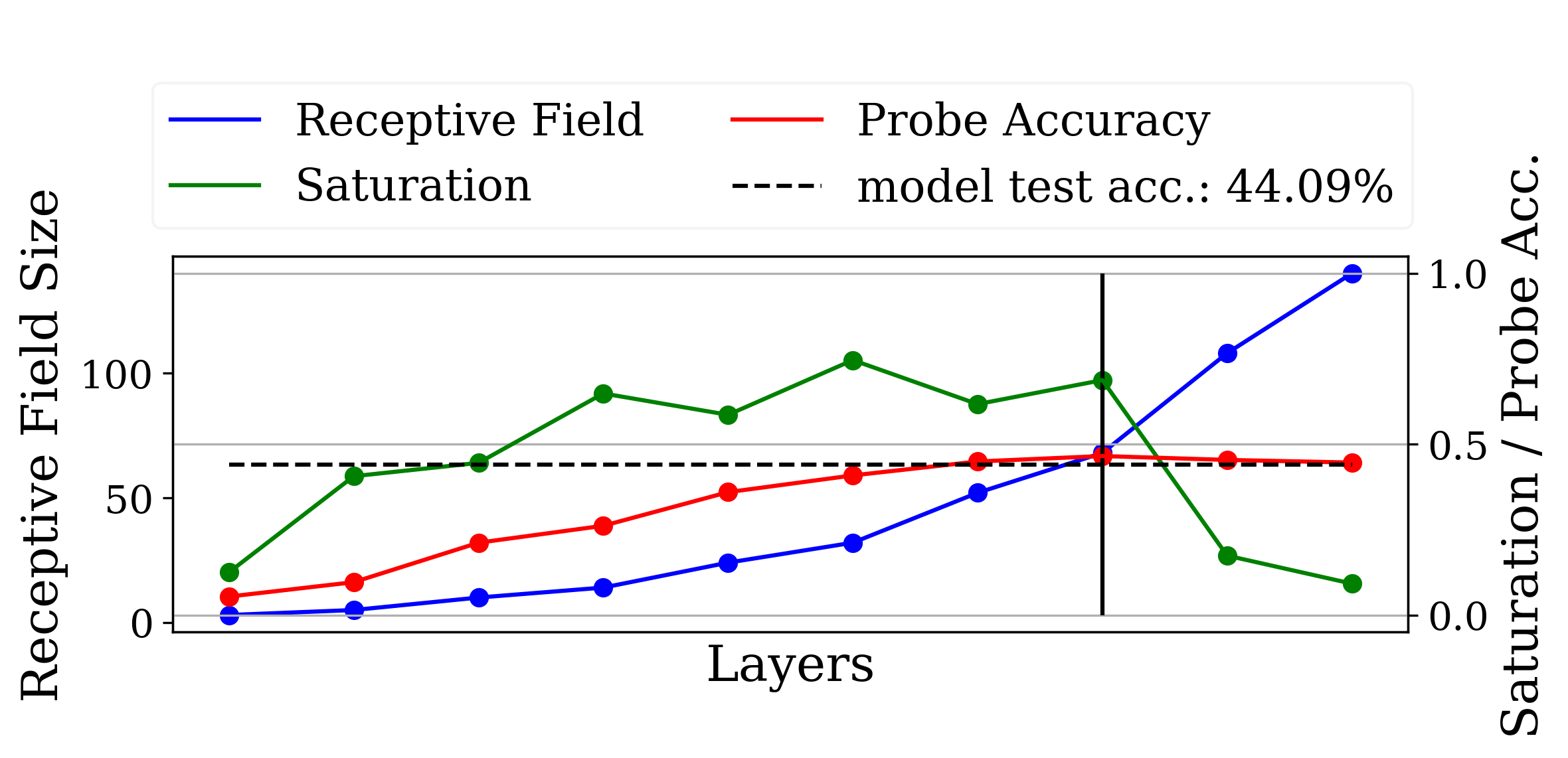
(b) VGG13

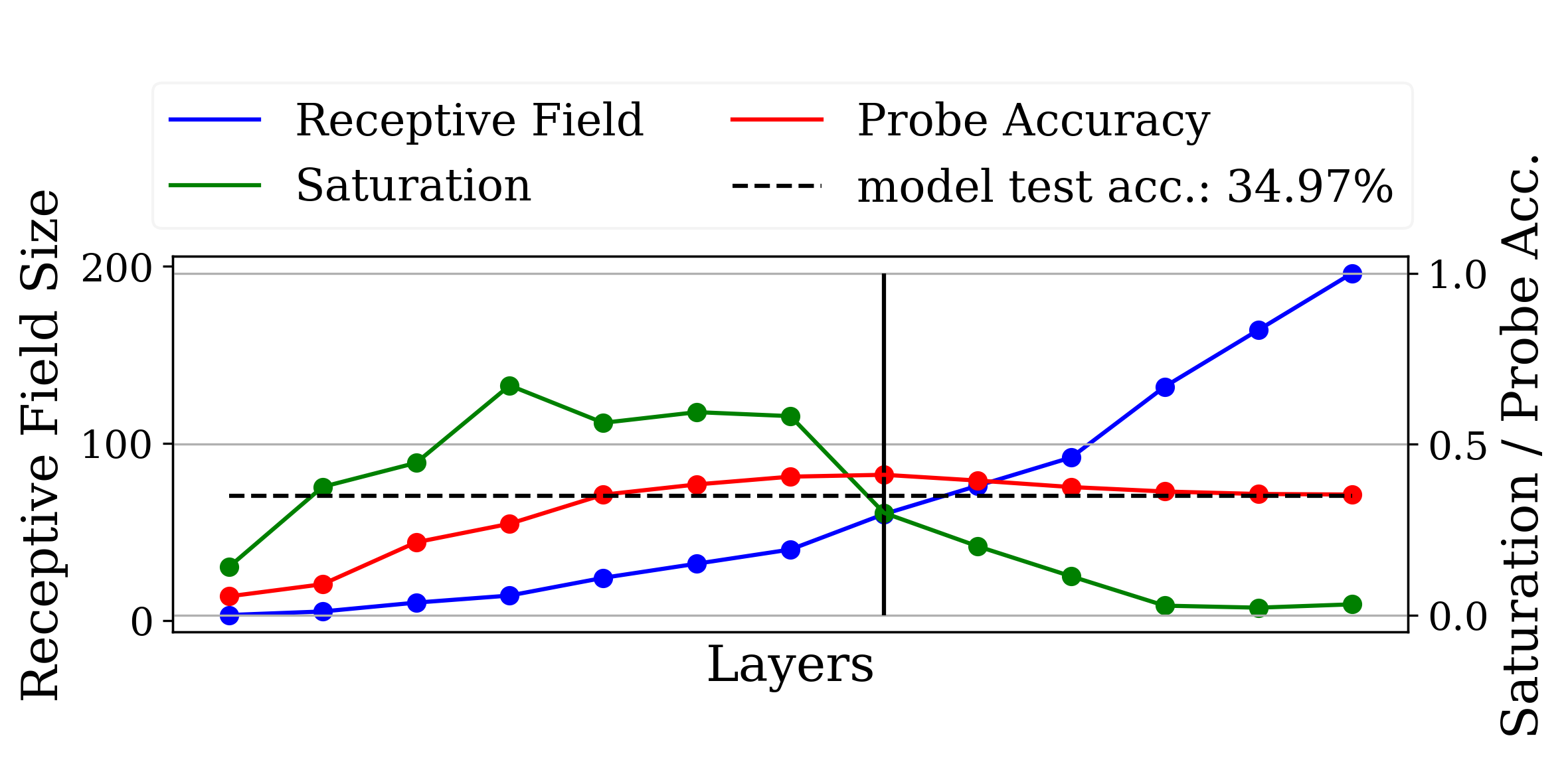
(c) VGG16

Figure 15: The first convolutional layer processing input from a layer with a receptive field size greater than the input size marks a border between an ”productive” and an ”unproductive” part of the network. Productive meaning relatively high saturated and visible improving probe performance. The depicted models are from the VGG-family of networks by Simonyan & Zisserman (2014) and trained on Cifar10 with an input size of $32\times 32$ pixels.

E.2 MNIST results

(a) VGG11

(b) VGG13

(c) VGG16

(d) VGG19

Figure 16: The first convolutional layer processing input from a layer with a receptive field size greater than the input size marks a border between an ”productive” and an ”unproductive” part of the network. Productive meaning relatively high saturated and visible improving probe performance. The depicted models are from the VGG-family of networks by Simonyan & Zisserman (2014) and trained on MNIST with an input size of $32\times 32$ pixels.

E.3 ResNet18 Cifar10 - Effect of disabling residual connections

Results indicate that removing the first three residual connections harms performance. Removing the last or second-to-last skip connection is statistically indistinguishable from not removing any residual connections. Furthermore, removing the first skip connection harms performance relative to many other permutations of residual connections. Thus, it seems like early downsampling decreases network performance and the first skip connection mitigates that effect. Later residual connections do not have the same effect.

	2,3,4	1,3,4	1,2,4	1,2,3	3,4	2,4	2,3	1,4	1,3	1,2	4	1	ResNet18
Mean	82.70	83.17	83.40	83.39	82.67	82.35	82.59	83.42	81.88	82.95	81.65	82.92	83.16
n	10	10	10	10	10	10	10	10	10	9	9	8	8

Table 2: ResNet18 with some residual connections removed. ResNet18 has four residual connections, bold numbers indicate which residual connections were enabled. For instance, 2, 3, 4 indicates that residual connections 2, 3 and 4 were present in the network. Mean performance of n Cifar10 trainings.

	2,3,4	1,3,4	1,2,4	1,2,3	3,4	2,4	2,3	1,4	1,3	1,2	4	1	ResNet18
2,3,4		0.026	0.004	0.015	0.879	0.340	0.638	0.001	0.563	0.256	0.014	0.287	0.260
1,3,4	-2.421		0.254	0.380	0.018	0.028	0.013	0.167	0.363	0.273	0.001	0.177	0.983
1,2,4	-3.297	-1.178		0.963	0.003	0.008	0.002	0.933	0.288	0.051	0.000	0.030	0.562
1,2,3	-2.701	-0.901	0.047		0.011	0.014	0.008	0.907	0.294	0.113	0.001	0.087	0.609
3,4	0.154	2.615	3.480	2.847		0.385	0.740	0.001	0.579	0.198	0.016	0.219	0.228
2,4	0.981	2.387	2.960	2.720	0.891		0.520	0.006	0.746	0.121	0.169	0.149	0.130
2,3	0.479	2.761	3.570	2.989	0.337	-0.656		0.001	0.617	0.135	0.028	0.153	0.179
1,4	-3.746	-1.438	-0.085	-0.119	-3.958	-3.113	-3.986		0.282	0.026	0.000	0.011	0.522
1,3	0.589	0.933	1.095	1.080	0.565	0.329	0.508	1.109		0.475	0.879	0.513	0.432
1,2	-1.176	1.132	2.098	1.673	-1.341	-1.632	-1.569	2.447	-0.731		0.005	0.884	0.617
4	2.750	4.126	4.613	4.264	2.671	1.437	2.402	4.819	0.154	3.291		0.007	0.014
1	-1.102	1.412	2.384	1.821	-1.279	-1.515	-1.502	2.888	-0.670	0.149	-3.136		0.579
ResNet18	-1.167	0.021	0.592	0.522	-1.253	-1.595	-1.407	0.655	-0.805	-0.510	-2.779	-0.568

Table 3: Independent two-sample t-test, pairwise mean performance difference significance test, ResNet18 with some residual connections removed, trained on Cifar10. ResNet18 has four skip-connections, bold numbers indicate which residual connections were enabled. For instance, 2, 3, 4 indicates that residual connections 2, 3 and 4 were present in the network. P-values are in the upper triangle, t-values in the lower. Statistically significant values (p¡0.25) are highlighted in green. n=10 or as in the previous table.

Appendix F Receptive Field Analysis with Partial Solution Heatmaps

F.1 Receptive Field Analysis using Probes on VGG16

(a) VGG16 trained on Cifar10 using $32\times 32$ pixel input size

(b) Conv1

(c) Conv2

(d) Conv3

(e) Conv4

(f) Conv5

(g) Conv6

(h) Conv7

(i) Conv8

(j) Conv9

(k) Conv10

(l) Conv11

(m) Conv12

(n) Conv13

(o)

Figure 17: VGG16 trained on Cifar10 alongside the heatmaps generated from the relative accuracy of the partial solutions in each layer. Note that the border layer (Conv8) is the first layer to have partial solutions of equal quality to the models solution (measured in accuracy).

F.2 Receptive Field Analysis using Probes on ResNet18

(a) ResNet18 trained on Cifar10 using $32\times 32$ pixel input size

(b) Conv1

(c) Block1-Conv1

(d) Block1-Conv2

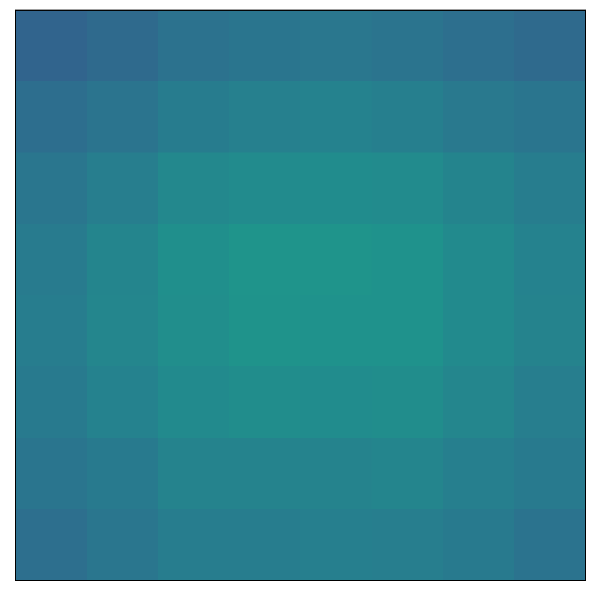
(e) Block2-Conv1

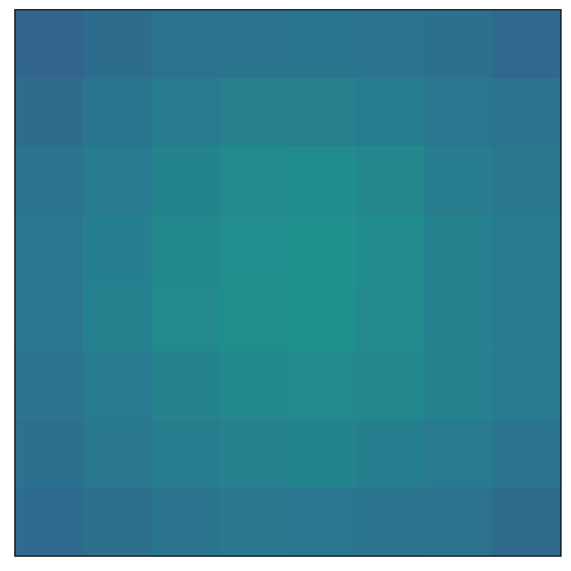
(f) Block2-Conv2

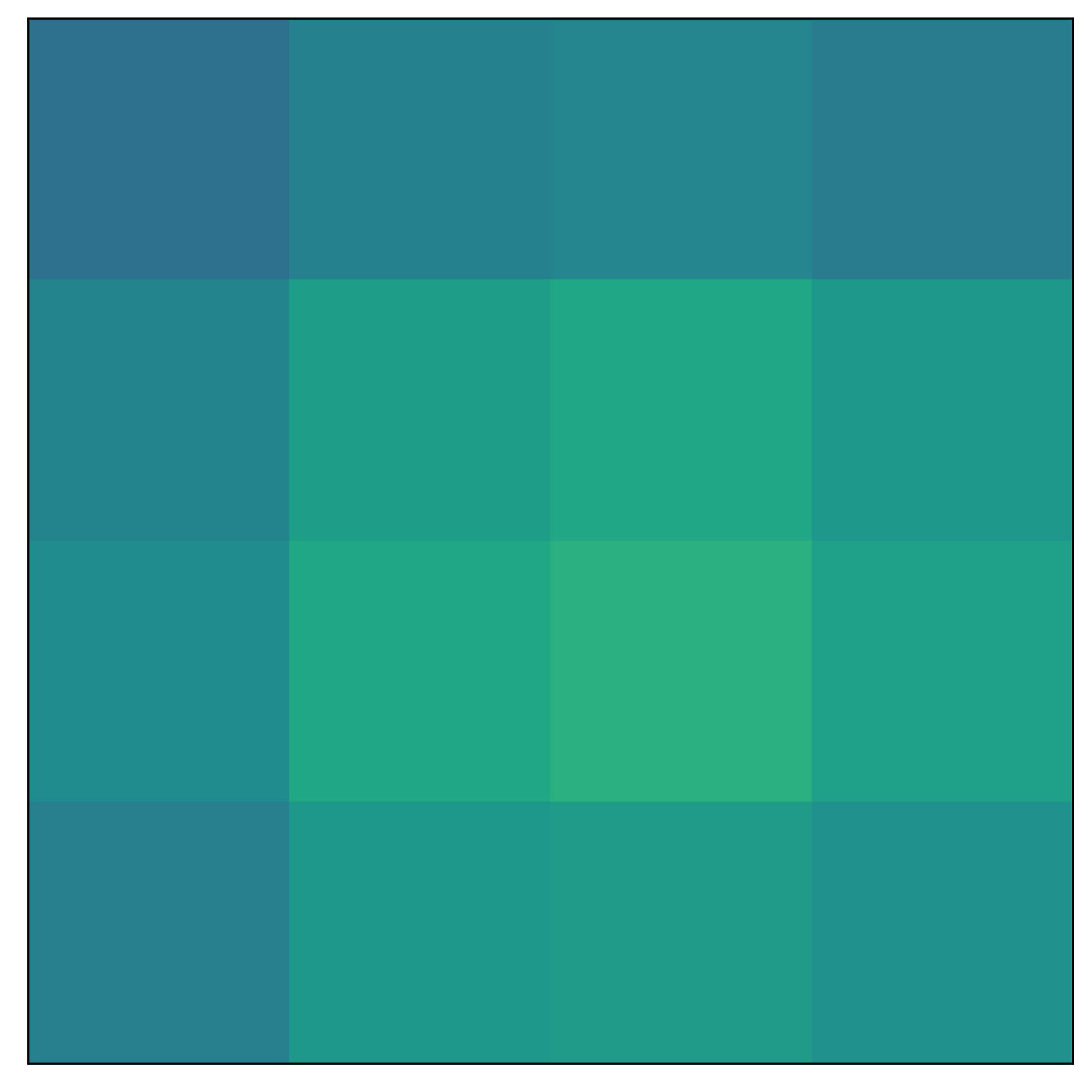
(g) Block3-Conv1

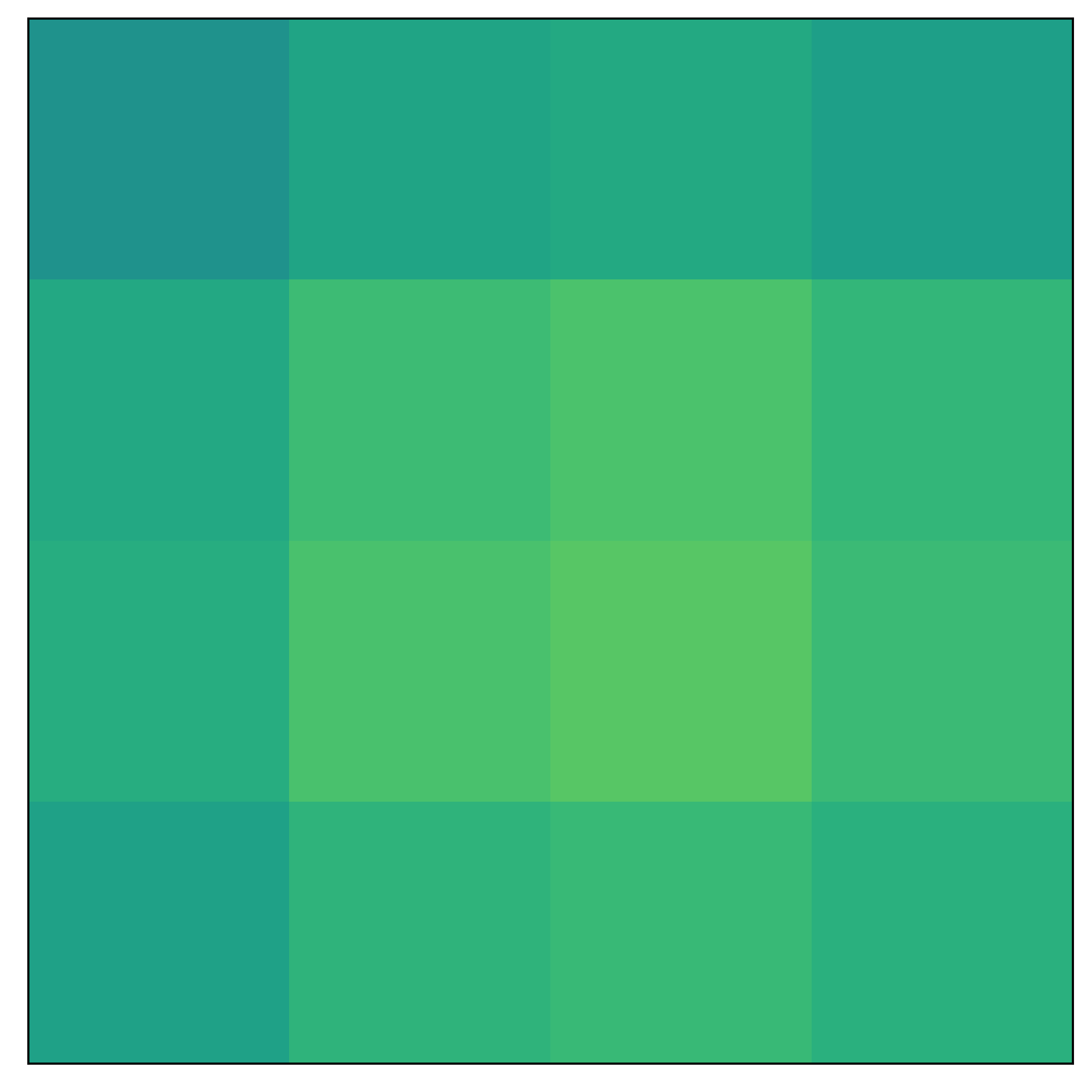
(h) Block3-Conv2

(i) Block4-Conv1

(j) Block4-Conv2

(k) Block5-Conv1

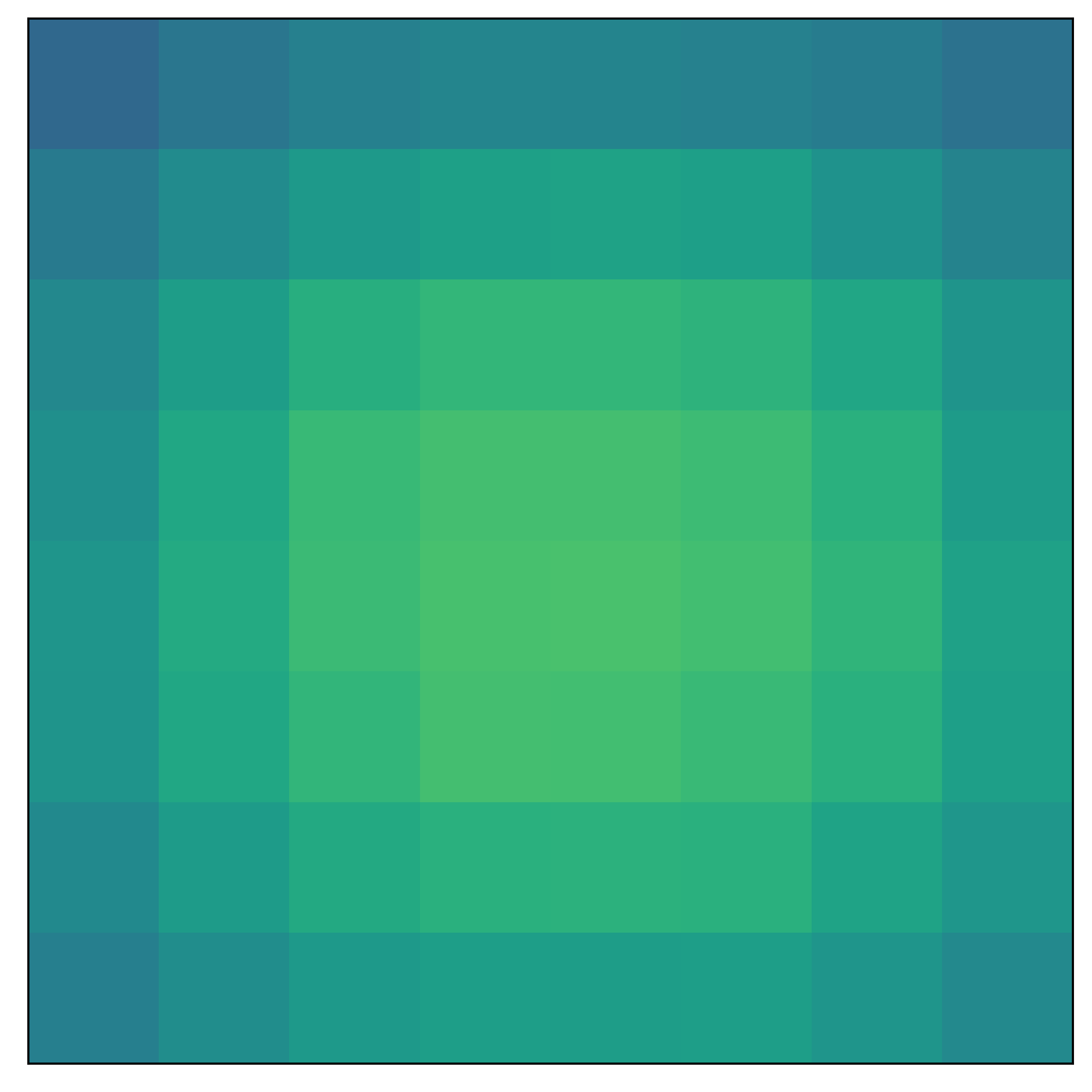
(l) Block5-Conv2

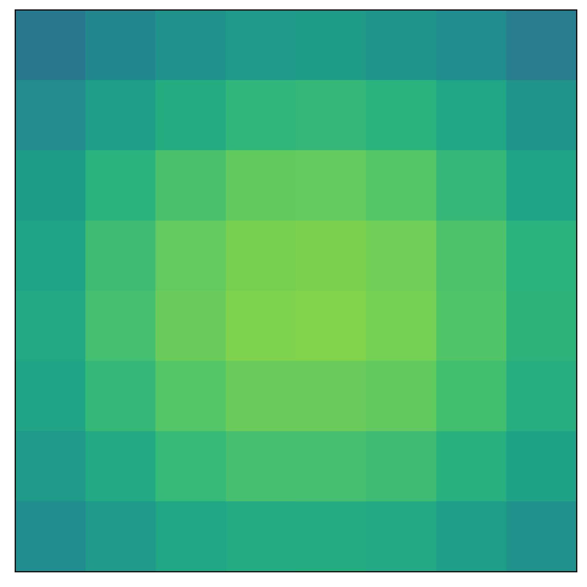
(m) Block6-Conv1

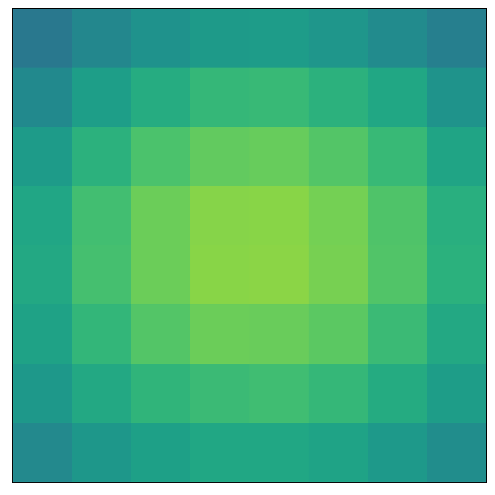
(n) Block6-Conv2

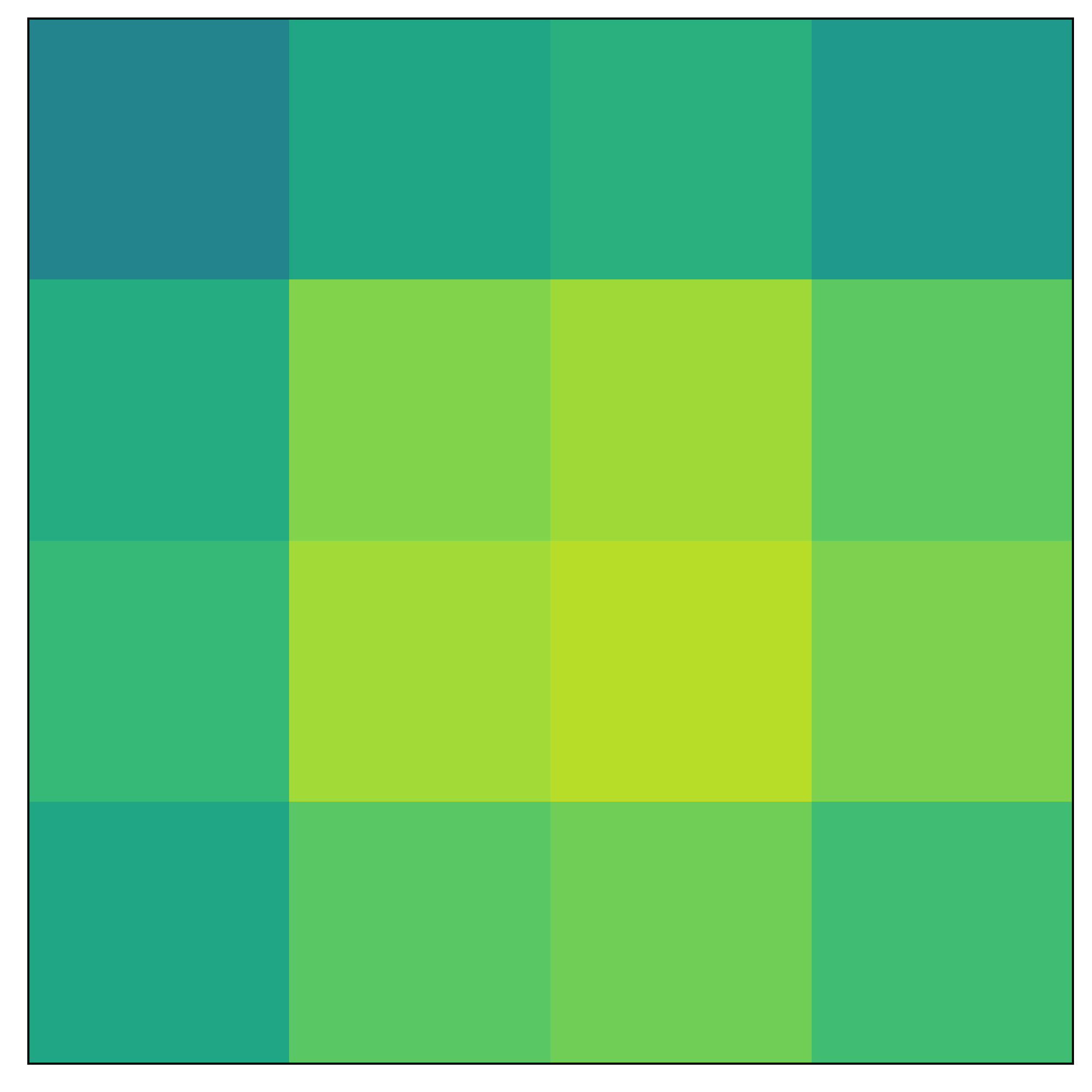
(o) Block7-Conv1

(p) Block7-Conv2

(q) Block8-Conv1

(r) Block8-Conv2

(s)

Figure 18: ResNet18 trained on Cifar10 alongside the heatmaps generated from the relative accuracy of the partial solutions in each layer. Note that ”skipped” layer (Block6-Conv2 and Block8-Con2) have a worse performance and worst partial solutions.

F.3 Receptive Field Analysis using Probes on ResNet18 optimized for Cifar10

(a) ResNet18 (Cifar10 Optimized) trained on Cifar10 using $32\times 32$ pixel input size

(b) Conv1

(c) Block1-Conv1

(d) Block1-Conv2

(e) Block2-Conv1

(f) Block2-Conv2

(g) Block3-Conv1

(h) Block3-Conv2

(i) Block4-Conv1

(j) Block4-Conv2

(k) Block5-Conv1

(l) Block5-Conv2

(m) Block6-Conv1

(n) Block6-Conv2

(o) Block7-Conv1

(p) Block7-Conv2

(q) Block8-Conv1

(r) Block8-Conv2

(s)

Figure 19: Cifar10 optimized ResNet18 trained on Cifar10 alongside the heatmaps generated from the relative accuracy of the partial solutions in each layer. Note that no layers are skipped and the solution quality of the partial solution develops up until the final residual block.

References

- Alain & Bengio (2016) Alain, G. and Bengio, Y. Understanding intermediate layers using linear classifier probes. ArXiv, abs/1610.01644, 2016.
- Bochkovskiy et al. (2020) Bochkovskiy, A., Wang, C.-Y., and Liao, H.-Y. M. YOLOv4: Optimal speed and accuracy of object detection, 2020.
- Bossard et al. (2014) Bossard, L., Guillaumin, M., and Van Gool, L. Food-101 – mining discriminative components with random forests. In Fleet, D., Pajdla, T., Schiele, B., and Tuytelaars, T. (eds.), Computer Vision – ECCV 2014, pp. 446–461, Cham, 2014. Springer International Publishing. ISBN 978-3-319-10599-4.
- Han et al. (2016) Han, D., Kim, J., and Kim, J. Deep pyramidal residual networks. CoRR, abs/1610.02915, 2016. URL http://arxiv.org/abs/1610.02915.
- He et al. (2015) He, K., Zhang, X., Ren, S., and Sun, J. Deep residual learning for image recognition. CoRR, abs/1512.03385, 2015.
- Horn et al. (2017) Horn, G. V., Aodha, O. M., Song, Y., Shepard, A., Adam, H., Perona, P., and Belongie, S. J. The iNaturalist challenge 2017 dataset. CoRR, abs/1707.06642, 2017. URL http://arxiv.org/abs/1707.06642.
- Huang et al. (2018) Huang, Y., Cheng, Y., Chen, D., Lee, H., Ngiam, J., Le, Q. V., and Chen, Z. Gpipe: Efficient training of giant neural networks using pipeline parallelism. CoRR, abs/1811.06965, 2018. URL http://arxiv.org/abs/1811.06965.
- Iandola et al. (2014) Iandola, F. N., Moskewicz, M. W., Karayev, S., Girshick, R. B., Darrell, T., and Keutzer, K. DenseNet: Implementing efficient convnet descriptor pyramids. CoRR, abs/1404.1869, 2014. URL http://arxiv.org/abs/1404.1869.
- Iandola et al. (2016) Iandola, F. N., Moskewicz, M. W., Ashraf, K., Han, S., Dally, W. J., and Keutzer, K. SqueezeNet: AlexNet-level accuracy with 50x fewer parameters and <1mb model size. CoRR, abs/1602.07360, 2016. URL http://arxiv.org/abs/1602.07360.
- Krizhevsky et al. (2010) Krizhevsky, A., Nair, V., and Hinton, G. CIFAR-10 (canadian institute for advanced research), 2010. URL http://www.cs.toronto.edu/~kriz/cifar.html.
- Krizhevsky et al. (2012) Krizhevsky, A., Sutskever, I., and Hinton, G. E. ImageNet classification with deep convolutional neural networks. In Pereira, F., Burges, C. J. C., Bottou, L., and Weinberger, K. Q. (eds.), Advances in Neural Information Processing Systems 25, pp. 1097–1105. Curran Associates, Inc., 2012.
- Le & Yang (2015) Le, Y. and Yang, X. Tiny ImageNet visual recognition challenge, 2015.
- LeCun & Cortes (2010) LeCun, Y. and Cortes, C. MNIST handwritten digit database. http://yann.lecun.com/exdb/mnist/, 2010. URL http://yann.lecun.com/exdb/mnist/.
- Lin et al. (2013) Lin, M., Chen, Q., and Yan, S. Network in network, 2013. URL http://arxiv.org/abs/1312.4400. cite arxiv:1312.4400Comment: 10 pages, 4 figures, for iclr2014.
- Redmon & Farhadi (2016) Redmon, J. and Farhadi, A. YOLO9000: better, faster, stronger. CoRR, abs/1612.08242, 2016. URL http://arxiv.org/abs/1612.08242.
- Redmon & Farhadi (2018) Redmon, J. and Farhadi, A. YOLOv3: An incremental improvement. CoRR, abs/1804.02767, 2018. URL http://arxiv.org/abs/1804.02767.
- Redmon et al. (2015) Redmon, J., Divvala, S. K., Girshick, R. B., and Farhadi, A. You only look once: Unified, real-time object detection. CoRR, abs/1506.02640, 2015. URL http://arxiv.org/abs/1506.02640.
- Richter et al. (2020) Richter, M. L., Shenk, J., Byttner, W., Arpteg, A., and Huss, M. Feature space saturation during training, 2020.
- Russakovsky et al. (2015) Russakovsky, O., Deng, J., Su, H., Krause, J., Satheesh, S., Ma, S., Huang, Z., Karpathy, A., Khosla, A., Bernstein, M., Berg, A. C., and Fei-Fei, L. ImageNet large scale visual recognition challenge. International Journal of Computer Vision (IJCV), 115(3):211–252, 2015. doi: 10.1007/s11263-015-0816-y.
- Simonyan & Zisserman (2014) Simonyan, K. and Zisserman, A. Very deep convolutional networks for large-scale image recognition. CoRR, abs/1409.1556, 2014.
- Szegedy et al. (2015) Szegedy, C., Liu, W., Jia, Y., Sermanet, P., Reed, S., Anguelov, D., Erhan, D., Vanhoucke, V., and Rabinovich, A. Going deeper with convolutions. In Proceedings of the IEEE Conference on Computer Vision and Pattern Recognition (CVPR), June 2015.
- Szegedy et al. (2016) Szegedy, C., Vanhoucke, V., Ioffe, S., Shlens, J., and Wojna, Z. Rethinking the inception architecture for computer vision. In IEEE Conference on Computer Vision and Pattern Recognition (CVPR), pp. 2818–2826, 2016. doi: 10.1109/CVPR.2016.308.
- Tan & Le (2019) Tan, M. and Le, Q. EfficientNet: Rethinking model scaling for convolutional neural networks. In Chaudhuri, K. and Salakhutdinov, R. (eds.), Proceedings of the 36th International Conference on Machine Learning, volume 97 of Proceedings of Machine Learning Research, pp. 6105–6114. PMLR, 09–15 Jun 2019.
- Zhang et al. (2017) Zhang, X., Zhou, X., Lin, M., and Sun, J. ShuffleNet: An extremely efficient convolutional neural network for mobile devices. CoRR, abs/1707.01083, 2017. URL http://arxiv.org/abs/1707.01083.