Iterated Kalman Methodology For Inverse Problems

Abstract

This paper is focused on the optimization approach to the solution of inverse problems. We introduce a stochastic dynamical system in which the parameter-to-data map is embedded, with the goal of employing techniques from nonlinear Kalman filtering to estimate the parameter given the data. The extended Kalman filter (which we refer to as ExKI in the context of inverse problems) can be effective for some inverse problems approached this way, but is impractical when the forward map is not readily differentiable and is given as a black box, and also for high dimensional parameter spaces because of the need to propagate large covariance matrices. Application of ensemble Kalman filters, for example use of the ensemble Kalman inversion (EKI) algorithm, has emerged as a useful tool which overcomes both of these issues: it is derivative free and works with a low-rank covariance approximation formed from the ensemble. In this paper, we work with the ExKI, EKI, and a variant on EKI which we term unscented Kalman inversion (UKI).

The paper contains two main contributions. Firstly, we identify a novel stochastic dynamical system in which the parameter-to-data map is embedded. We present theory in the linear case to show exponential convergence of the mean of the filtering distribution to the solution of a regularized least squares problem. This is in contrast to previous work in which the EKI has been employed where the dynamical system used leads to algebraic convergence to an unregularized problem. Secondly, we show that the application of the UKI to this novel stochastic dynamical system yields improved inversion results, in comparison with the application of EKI to the same novel stochastic dynamical system.

The numerical experiments include proof-of-concept linear examples and various applied nonlinear inverse problems: learning of permeability parameters in subsurface flow; learning the damage field from structure deformation; learning the Navier-Stokes initial condition from solution data at positive times; learning subgrid-scale parameters in a general circulation model (GCM) from time-averaged statistics.

1 Introduction

1.1 Overview

This paper is devoted to optimization approaches to calibrating models with observational data. The basic problem is formulated as recovering unknown model parameters $\theta\in\mathbb{R}^{N_{\theta}}$ from noisy observation $y\in\mathbb{R}^{N_{y}}$ given by

$$y=\mathcal{G}(\theta)+\eta;$$ (1)

here $\mathcal{G}$ denotes the parameter-to-data map which, for the applications we have in mind, generally requires solving partial differential equations, and $\eta\sim\mathcal{N}(0,\Sigma_{\eta})$ denotes the Gaussian observation error. Consider now the stochastic dynamical system

evolution: $$\theta_{n+1}=\alpha\theta_{n}+(1-\alpha)r_{0}+\omega_{n+1}, \omega_{n+1}\sim\mathcal{N}(0,\Sigma_{\omega}),$$ (2a)

observation: $$y_{n+1}=\mathcal{G}(\theta_{n+1})+\nu_{n+1}, \nu_{n+1}\sim\mathcal{N}(0,\Sigma_{\nu}).$$ (2b)

We assume that the artificial evolution error covariance $\Sigma_{\omega}\succ 0$, the artificial observation error covariance $\Sigma_{\nu}\succ 0$, and the regularization parameter $\alpha\in(0,1]$, whilst $r_{0}$ is an arbitrary vector. We study methods to determine $\theta$ from $y$ given by (1) by employing filtering methods to find $\theta_{n}$ given $Y_{n}:=\{y_{\ell}\}_{\ell=1}^{n}$, in the setting where $y_{\ell}\equiv y$ for all $\ell\in\mathbb{N}.$

Note that dynamical system (2a) for $\theta_{n}$ has, for $\alpha\in(0,1)$, statistical equilibrium given by the Gaussian $\mathcal{N}(r_{0},(1-\alpha^{2})^{-1}\Sigma_{\omega}).$ The output of this statistical model is then repeatedly exposed to the observations, expressed via (2b) with $y_{n+1}$ set to the data $y$, and hence it is intuitive that filtering methods will deliver an estimate of $\theta$ solving (1) as $n\to\infty.$ Such a method, in the special case $\alpha=1,\Sigma_{\omega}=0,\Sigma_{\nu}=\Sigma_{\eta}$, is the basis of the ensemble Kalman inversion (EKI) algorithm as proposed in [1]. The two main takeaway messages of this paper are firstly to highlight the benefits of choosing $\alpha\in(0,1)$ and $\Sigma_{\omega}\succ 0$, and secondly to demonstrate that application of the unscented Kalman filter improves on the ensemble Kalman filter, leading to unscented Kalman inversion (UKI).

The primary issue with the choice $\alpha=1$ is that it leads to over-fitting for problems in which $N_{\theta}>N_{y}$, as shown in [1]. One approach to deal with this is to use an adaptive modification of the basic EKI algorithm, based on an analogy with the Levenberg-Marquardt algorithm, as developed in [2]; however, this leads to a need for stopping criterion and the area is still being developed [3]. Another approach is to build Tikhonov regularization directly into the inverse problem, before applying a filtering algorithm to (2) with $\alpha=1,\Sigma_{\omega}=0$, an approach introduced in [4]. However, this leads to an algorithm which requires the inversion of covariance matrices on spaces of dimension $N_{\theta}+N_{y}$ which is undesirable for many problems concerning inference about fields, where $N_{\theta}\gg 1.$ This issue is removed if the continuum limit of the algorithm is used [4]. However, practical experience with using time-steppers for continuum limits of ensemble Kalman filtering algorithms is in its infancy and current implementations of the methods in [4, 5, 6, 7, 8] are not competitive with algorithms which start directly from a discrete time formulation.

Central to both the optimization and probabilistic approaches to inversion is the regularized objective function $\Phi_{R}(\theta)$ defined by

$$\Phi_{R}(\theta) :=\Phi(\theta)+\frac{1}{2}\lVert\Sigma_{0}^{-\frac{1}{2}}(\theta-r_{0})\rVert^{2},$$ (3a)

$$\Phi(\theta) :=\frac{1}{2}\lVert\Sigma_{\eta}^{-\frac{1}{2}}(y-\mathcal{G}(\theta))\rVert^{2},$$ (3b)

where $\Sigma_{\eta}\succ 0$ normalizes the model-data misfit $\Phi$ by means of the known error statistics of the noise, prior mean $r_{0}$ encodes prior information about $\theta$, and prior covariance $\Sigma_{0}\succ 0$ normalizes the prior information. We will connect the parameters of (2) for $\theta$ to a form of regularization of the inverse problem. In this context it is worth noticing that, for linear problems, the implied Tikhonov regularization has implied mean $r_{0}$, whilst the implied covariance $\Sigma_{0}$ of the regularization term is defined implicitly via limit of an iterative procedure. Parameter $\alpha\in(0,1)$ controls the size of the regularization effect; and when $\alpha=1$ the regularization effect disappears, along with dependence of (2a) on $r_{0}$. Thus $\alpha=1$ is useful primarily for over-determined problems.

1.2 Our Contributions

We make the following contributions to the study of the solution of inverse problems by means of filtering methods:

• we introduce a filtering-based approach to solving the inverse problem (1), based on the novel stochastic dynamical system formulation (2);

• by studying linear problems we demonstrate that the methodology induces a form of Tikhonov regularization and we prove an exponential convergence of the algorithm to the minimizer of the Tikhonov-regularized problem, in the linear case;

• we introduce a Gaussian approximation for the filtering distribution defined by (2) and, from it, derive extended Kalman, ensemble Kalman and unscented Kalman (ExKI, EKI and UKI respectively) algorithms for the inverse problem (1), applicable in the general nonlinear case;

• the algorithms are tested on a wide range of problems, including linear test problems, inversion for spatial fields in a variety of continuum mechanics applications, and the learning of parameters in chaotic dynamical systems, using time-averaged data;

• we show that UKI outperforms EKI, with both employed in the context of the stochastic dynamical model (2), for a wide range of inverse problems with unknown parameter space of moderate dimension.

Taken together, the theoretical framework we develop and the numerical results we present show that the UKI, applied to the stochastic dynamical system (2), is a competitive methodology for solving inverse problems and parameter estimation problems defined by an expensive black-box forward model; indeed the UKI is shown to outperform the EKI in settings where the number of parameters $N_{\theta}$ is of moderate size and the black-box is not readily differentiable so that ExKI methods are not applicable. Other ensemble filters, such as the ensemble adjustment and ensemble transform Kalman filters could also be used in place of unscented Kalman filters, and similar performance is to be expected. This issue is explored in detail in [9] where ideas introduced in this paper are developed further in order to approximate the Bayesian posterior distribution for inverse problem (1). We note that, as with the use of most nonlinear variants of the Kalman filter, rigorous justification beyond the linear setting is not currently available, but that our numerical results demonstrate effectiveness in a wide range of nonlinear inverse problems. The use of interacting particle systems to solve inverse problems with multimodal distributions, far from Gaussian, is considered in [10] and the derivation of mean-field limits of ensemble Kalman methods for inversion, viewed as interacting particle systems is established in [11, 12].

We conclude this introductory section with a deeper literature review relating to the contributions we make in this paper, in Subsection 1.3. Then, in Section 2 we introduce a conceptual algorithm based on a Gaussian approximation of the filtering distribution associated with (2); we then derive the ExKI, UKI, and EKI algorithms as approximations to this conceptual Gaussian algorithm. In Section 3 we study the methodology for linear problems, obtaining insight into the regularization conferred by (2a); we study the relationship of the methodology to other gradient-based optimization techniques; we derive continuous-time limits in the nonlinear setting. Section 4 describes variants on the basic conceptual algorithm that may be useful in some settings, and in Section 5 we present numerical results demonstrating the performance of the inversion methodology introduced in this paper. The code relating to numerical experiments presented in Section 5 is accessible online:

https://github.com/Zhengyu-Huang/InverseProblems.jl

1.3 Literature Review

The focus of this paper is mainly on derivative-free inversion by means of iterative techniques aimed at solving the optimization problem defined by minimization of $\Phi_{R}$, or variants of this problem [13]. However, even in the optimization setting, the methods introduced in this paper are closely related to iterative methods applied in Bayesian (probabilistic) inversion. In the Bayesian approach to the inverse problem (1) [14, 15] the posterior distribution is given by

$$\mu(d\theta)=\frac{1}{Z}\exp\bigl{(}-\Phi(\theta)\bigr{)}\mu_{0}(d\theta),$$ (4)

where $\mu_{0}=\mathcal{N}(r_{0},\Sigma_{0})$ is the prior and $\mu$ is the posterior. A commonly adopted iterative approach to solving the problem of sampling from $\mu$ is the finite time approach known as sequential Monte Carlo (SMC) – see [16, 17], and [18] for applications to inverse problems. The basic idea, upon which there are many variants, is to consider the sequence of measures $\mu_{n}$ defined by

$$\mu_{n+1}(d\theta)=\frac{1}{Z_{n}}\exp\bigl{(}-h\Phi(\theta)\bigr{)}\mu_{n}(d\theta).$$ (5)

Note, then, that if $Nh=1$ it follows that $\mu_{N}=\mu.$ Each step $\mu_{n}\mapsto\mu_{n+1}$ may be approximated by a particle-based filtering algorithm, leading to a variety of algorithms used in practice, involving a fixed finite number of steps $N$. Furthermore, continuous-time limits of this methodology may also be derived by taking $N\to\infty$ and $h\to 0$ with $Nh=1$, giving insight into the algorithms; see [19, 8].

On the other hand, if $h=1$ is fixed and the measures $\mu_{n}$ are studied in the limit $n\to\infty$, they will tend to concentrate on minimizers of $\Phi$, restricted to the support of $\mu_{0}$, as the following identity shows:

$$\mu_{n}(d\theta)=\frac{1}{\bigl{(}\Pi_{\ell=0}^{n-1}Z_{\ell}\bigr{)}}\exp\bigl{(}-n\Phi(\theta)\bigr{)}\mu_{0}(d\theta).$$ (6)

This corresponds to an infinite time approach.

The finite time approach was developed for probabilistic problems; the infinite time approach is focused on optimization. This paper will build on the latter, optimization, approach to the problem. However, we note that, other than restriction of $\mu_{n}$ to the support of $\mu_{0}$, regularization is lost in this approach since it focuses on minimizing $\Phi(\cdot)$ and not $\Phi_{R}(\cdot)$. To introduce regularization we consider the iteration

$$\mu_{n+1}(d\theta)=\frac{1}{Z_{n}}\exp\bigl{(}-\Phi(\theta)\bigr{)}P_{n}\mu_{n}(d\theta).$$ (7)

To address the issue of regularization, we will choose $P_{n}$ to be the Markov kernel associated with a first-order autoregressive (AR1) process as defined by (2a); it is thus independent of $n:P_{n}\equiv P.$ The resulting dynamic on measures $\mu_{n}$ defined by (7) corresponds to the filtering distribution for $\theta_{n}|Y_{n}$ defined by the stochastic dynamical system (2). We note that within SMC $P_{n}$ is also introduced in a similar fashion in (5), but in that context it is chosen to be a $\mu_{n}-$invariant Markov kernel so that $P_{n}\mu_{n}=\mu_{n}$, typically from MCMC; in this setting $P_{n}$ is indeed $n-$dependent. Note that $\mu_{n}$ is not invariant with respect to $P$ with the AR1 choice we make: thus the introduction of $P_{n}$ in our setting differs from its use in SMC; this is because we are solving an optimization problem via iteration over $n$, and not the sampling problem which morphs the prior at time $n=0$ into the posterior at time $n=N.$ The specific choice of $P_{n}$ made in our work, namely the Markov kernel $P$ defined by an AR1 process, is made in order to regularize the iterative optimization approach to inversion encapsulated in (6). Once we apply particle methods, the presence of $P$ plays the role of avoiding ensemble collapse [5, 6, 4]. We also note that, in contrast to SMC, the initial measure $\mu_{0}$ in (7) does not need to be the prior distribution – it may be chosen arbitrarily, although a natural choice is the stationary measure for the AR1 process.

In the case where $\mathcal{G}$ is linear, (7) delivers a sequence of measures, which are defined through a Kalman filter. Our analysis of the underlying filtering problem in Subsection 3.1, which considers the linear Gaussian setting, thus constitutes an analysis of the Kalman filter for a specific state-space model with a specific choice of data. In order to deal with a range of cases, including exponential convergence, algebraic convergence and divergence of the mean/covariances of the filter, we introduce an explicit unified analysis of the Kalman filter in our setting. We note, however, that this is a well-trodden field and that variants on some of our results can be obtained from the existing literature [20, 21].

The method we introduce and study in this paper arises from the application of ideas from Kalman filtering to the problem of approximating the distribution of $\theta_{n}|Y_{n}$. The Kalman filter itself applies to the case of linear $\mathcal{G}$ [22, 23]. When $\mathcal{G}$ is nonlinear the methods can be generalized by use of the extended Kalman filter (ExKF) [24] which is based on linearization and application of Kalman methodology. However this method suffers from two drawbacks which hamper its application in many large-scale applications: (a) it requires a derivative of the forward map $\mathcal{G}(\cdot)$; and (b) the approach scales poorly to high dimensional parameter spaces where $N_{\theta}\gg 1$, because of the need to sequentially update covariances in $\mathbb{R}^{N_{\theta}\times N_{\theta}}.$ Thus, despite an early realization that Kalman-based methods could be useful for large-scale filtering problems arising in the geosciences [25], the methods did not become practical in this context until the work of Evensen [26]. This revolutionary paper introduced the ensemble Kalman filter (EnKF) the essence of which is to avoid the linearization of the dynamics and sequential updating of the covariance, and instead use a low-rank approximation of the covariance found by maintaining an ensemble of estimates for $\theta_{n}|Y_{n}$ at every step $n.$ These ensemble Kalman methods have been widely adopted in the geosciences, not only because they are effective for high dimensional parameter spaces, but also because they are derivative-free, requiring only $\mathcal{G}$ as a black box. Their use in the solution of inverse problems via iterative methods was pioneered in subsurface inversion [27, 28] where the perspective of fixing $h\ll 1$ and iterating until $n=N=1/h$ was used, so that $\mu_{N}$ is viewed as an approximation of the posterior, provided $\mu_{0}$ is chosen as the prior. These papers thus view the ensemble methodology as a way of sampling from the posterior and have elements in common with SMC; this idea is also implicit in the paper [19], which is focused on data assimilation, and addresses the solution of a Bayesian inverse problem each time new data is received.

In [1] the Kalman methodology for inversion was revisited from the optimization perspective, based on fixing $h=1$ and iterating in $n$, leading to an algorithm we will refer to as ensemble Kalman inversion (EKI). The paper [2] introduced a novel approach to regularizing the iterative method, by drawing an analogy with the Levenberg-Marquardt algorithm (LMA) [29]; see also [3]. Subsequent variants on the iterative optimization approach demonstrate how to introduce Tikhonov regularization into the EKI algorithm [4] and the paper [6] shows that adding noise to the iteration can lead to approximate Bayesian inversion, a method we will refer to as ensemble Kalman sampling (EKS) and which is further analyzed in [7, 30]. The EKS provides a different approach to the problem of Bayesian inversion from the ones pioneered in [27, 28] since it does not require starting with draws from the prior $\mu_{0}$, but instead relies on ergodicity and iteration to large $n$; the methods in [27, 28] must be started with draws from the prior $\mu_{0}$ and iterated for precisely $n=1/h$ steps, and are hence more rigid in their requirements. Since the ensemble methods do not, in general, accurately approximate the true posterior distribution [31, 32] outside Gaussian scenarios, the derivative-free optimization perspective is arguably a more natural avenue within which to analyze ensemble inversion. However recent work demonstrates how a derivative-free multiscale stochastic sampling method can usefully take the output of EKS as a preconditioner for a method which provably approximates the true posterior distribution [33]; in that context, the EKS is central to making the method efficient. Furthermore, in recent interesting work, it has been shown how to reweight ensemble Kalman methods to recover statistical consistency in the non-Gaussian setting [8]; however computation of the weights requires gradients of $\mathcal{G}$ and hence is not practical for many of the problems where ensemble methods are most useful.

Within the control theory literature, and parallel to the development of the ensemble Kalman filter, the unscented Kalman filter (UKF) was introduced [34, 35]. Like the ensemble Kalman methods, this method also sidesteps the need to sequentially update the derivative of the forward model as part of the covariance update; but, in the primary difference from ensemble Kalman methods, particles (sigma points) are chosen deterministically, and a quadrature rule is applied within a Gaussian approximation of the filter. This paper is to establish a framework for the development of unscented Kalman methods for inverse problems, based on (2): we formalize and demonstrate the power of unscented Kalman inversion (UKI) techniques. We also formalize extended Kalman inversion (ExKI) as a general purpose methodology for parameter learning and derive ExKI, UKI, and UKI as different approximations of a conceptual Gaussian methodology for the (in general non-Gaussian) filtering problem defined by (2).

Inverse and parameter estimation problems are ubiquitous in engineering and scientific applications. Applications that motivate this work include global climate model calibration [36, 37, 38], material constitutive relation calibration [39, 40, 41], seismic inversion in geophysics [42, 43], and medical tomography [44, 45]. These problems are generally highly nonlinear, may feature multiple scales, and may include chaotic and turbulent phenomena. Moreover, the observational data is often noisy and the inverse problem may be ill-posed. We note, also, that a number of inverse problems of interest may involve a moderate number of unknown parameters $N_{\theta}$, yet may involve the solution of a very expensive forward model $\mathcal{G}$ depending on those parameters; furthermore, $\mathcal{G}$ may not be differentiable with respect to the parameters, or may be complex to differentiate as it is given as a black box.

In the nonlinear setting of state estimation, there are three primary types of Kalman filters [46, 47, 48]: the extended Kalman filter (ExKF), the unscented Kalman filter (UKF), and the ensemble Kalman filter (EnKF). The use of Kalman based methodology as a non-intrusive iterative method for parameter estimation originates in the papers [49, 50] which were based on the ExKF, hence requiring derivative $d\mathcal{G}$, and its adjoint, to propagate covariances; the use of derivative-free ensemble methods was then developed systematically in the papers [27, 28], in the SMC context, followed by the iterate for optimization EKI approach [1]. Derivative-free ensemble inversion and parameter estimation are particularly suitable for complex multiphysics problems requiring coupling of different solvers, such as fluid-structure interaction [51, 52, 53, 54] and general circulation models [55] and methods containing discontinuities such as the immersed/embedded boundary method [56, 57, 58, 59] and adaptive mesh refinement [60, 61]. Furthermore, derivative-free ensemble inversion and parameter estimation has been demonstrated to be effective in the context of forward models defined by chaotic dynamical systems [62] where adjoint-based methods fail to deliver meaningful sensitivities [63, 64]. These wide-ranging potential applications form motivation for developing other derivative-free Kalman based inversion and parameter estimation techniques, and in particular, the unscented Kalman methods developed here.

There is already some work in which unscented Kalman methods are used for parameter inversion. Extended, ensemble and unscented Kalman inversions have been applied to train neural networks [49, 50, 35, 65] and EKI has been applied in the oil industry [66, 27, 28]. Dual and joint Kalman filters [67, 35] have been designed to simultaneously estimate the unknown states and the parameters [67, 68, 35, 69, 70] from noisy sequential observations. However, whilst the EKI has been systematically developed and analyzed as a general purpose methodology for the solution of inverse and parameter estimation problems, the same is not the case for UKI.

Continuous-time limits and gradient flow structure of the EKI have been introduced and studied in [19, 71, 5, 72, 73, 11, 12]. This work led to the development of variants on the EKI, such as the Tikhonov-EKI (TEKI) [4] and the EKS [6]. We will develop study of continuous-time limits for the UKI, and variants including an unscented Kalman sampler (UKS), in this paper. There are interesting links to the Levenberg–Marquardt Algorithm (LMA) [74, 29], as introduced in [2] and developed further in [75, 76, 3]. We will further refine the idea, which provides insights into understanding and improving the nonlinear Kalman inversion methodology as introduced here.

Finally, we mention that there are other derivative-free optimization techniques which are based on interacting particle systems, but are not Kalman based. Rather these methods are based on consensus-forming mean-field models, and their particle approximations, leading to consensus-based optimization [77] and consensus-based sampling [78]. The paper [33] also provides an alternative derivative-free approach to optimization and sampling for inverse problems, using ideas from multiscale dynamical systems.

2 Nonlinear Kalman Inversion Algorithms

Recall that the basic approach to inverse problems that we adopt in this paper is to pair the parameter-to-data relationship encoded in (1) with a stochastic dynamical system for the parameter, resulting in (2). We then employ techniques from filtering to approximate the distribution $\mu_{n}$ of $\theta_{n}|Y_{n}$. A useful way to think of updating $\mu_{n}$ is through the prediction and analysis steps [79, 80]: $\mu_{n}\mapsto\hat{\mu}_{n+1}$, and then $\hat{\mu}_{n+1}\mapsto\mu_{n+1}$, where $\hat{\mu}_{n+1}$ is the distribution of $\theta_{n+1}|Y_{n}$. In Subsection 2.1 we first introduce a Gaussian approximation of the analysis step, leading to an algorithm which maps the space of Gaussian measures into itself at each step of the iteration; it is not implementable in general, but it is a useful conceptual algorithm. Subsection 2.2 shows how this algorithm can be made practical, for low to moderate dimension $N_{\theta}$ and assuming that $d\mathcal{G}$ is available, by means of the ExKF, a form of linearization of the conceptual algorithm; we refer to this as ExKI. In Subsection 2.3 we show how the UKI algorithm may be derived by applying a quadrature rule to evaluate certain integrals appearing in the conceptual Gaussian approximation. Subsection 2.4 connects the conceptual algorithm with the EKI, an approach in which ensemble approximation of the integrals is used.

2.1 Gaussian Approximation

This conceptual algorithm maps Gaussians into Gaussians, and henceforth it is referred to as the Gaussian Approximation Algorithm (GAA). Assume that $\mu_{n}\approx\mathcal{N}(m_{n},C_{n})$. The GAA is a mapping from $(m_{n},C_{n})$ into $(m_{n+1},C_{n+1})$ which reduces to the Kalman filter in the linear setting. The algorithm proceeds by determining the joint distribution of $\theta_{n+1},y_{n+1}|Y_{n}$, assuming that $\theta_{n}|Y_{n}$ is Gaussian $\mathcal{N}(m_{n},C_{n})$. We then project this joint distribution onto a Gaussian by computing its mean and covariance. And finally, we compute the conditional distribution of this joint Gaussian on observed $y_{n+1}$ to obtain a Gaussian approximation $\mathcal{N}(m_{n+1},C_{n+1})$ to $\mu_{n+1},$ the distribution of $\theta_{n+1}|Y_{n+1}.$

The projection of the joint distribution of $\{\theta_{n+1},y_{n+1}\}|Y_{n}$ onto a Gaussian distribution has the form

$$\mathcal{N}\Bigl{(}\begin{bmatrix}\widehat{m}_{n+1}\\ \widehat{y}_{n+1}\end{bmatrix},\begin{bmatrix}\widehat{C}_{n+1}&\widehat{C}_{n+1}^{\theta y}\\ {{\widehat{C}_{n+1}}^{\theta y}}{}^{T}&\widehat{C}_{n+1}^{yy}\end{bmatrix}\Bigr{)};$$ (8)

we now define all the components of the mean and covariance. Note that, under (2a), $\hat{\mu}_{n+1}$ is also Gaussian if $\mu_{n}$ is Gaussian. The use of (2a) shows that

$$\begin{split}\widehat{m}_{n+1}&=\mathbb{E}[\theta_{n+1}|Y_{n}]=\alpha m_{n}+(1-\alpha)r_{0},\\ \widehat{C}_{n+1}&=\mathrm{Cov}[\theta_{n+1}|Y_{n}]=\alpha^{2}C_{n}+\Sigma_{\omega}.\end{split}$$ (9)

Then, with $\mathbb{E}$ denoting expectation with respect to $\theta_{n+1}|Y_{n}\sim\mathcal{N}(\widehat{m}_{n+1},\widehat{C}_{n+1})$, we have

$$\begin{split}\widehat{y}_{n+1}=&\mathbb{E}[\mathcal{G}(\theta_{n+1})|Y_{n}],\\ \widehat{C}_{n+1}^{\theta y}=&\mathrm{Cov}[\theta_{n+1},\mathcal{G}(\theta_{n+1})|Y_{n}],\\ \widehat{C}_{n+1}^{yy}=&\mathrm{Cov}[\mathcal{G}(\theta_{n+1})|Y_{n}]+\Sigma_{\nu}.\end{split}$$ (10)

Computing the conditional distribution of the joint Gaussian in (8) to find $\theta_{n+1}|\{Y_{n},y_{n+1}\}=\theta_{n+1}|Y_{n+1}$ gives the following expressions for the mean $m_{n+1}$ and covariance $C_{n+1}$ of the approximation to $\mu_{n+1}:$

$$\begin{split}m_{n+1}&=\widehat{m}_{n+1}+\widehat{C}_{n+1}^{\theta y}(\widehat{C}_{n+1}^{yy})^{-1}(y_{n+1}-\widehat{y}_{n+1}),\\ C_{n+1}&=\widehat{C}_{n+1}-\widehat{C}_{n+1}^{\theta y}(\widehat{C}_{n+1}^{yy})^{-1}{\widehat{C}_{n+1}^{\theta y}}{}^{T}.\end{split}$$ (11)

Equations (9), (10) and (11) define the GAA. As a method for solving the inverse problem (1), the GAA is implemented by assuming all observations $\{y_{n}\}$ are identical to $y$ and iterating in $n.$ With this assumption, we may write the algorithm as

$$(m_{n+1},C_{n+1})=F(m_{n},C_{n};\mathcal{G},r_{0},\Sigma_{\omega}),$$ (12)

noting that the mapping is dependent on $\mathcal{G}$ and on the mean and covariance of the assumed auto-regressive dynamics for $\{\theta_{n}\}$.

In the setting where $\mathcal{G}$ is linear, the Gaussian ansatz used in the derivation of the conceptual algorithm is exact, the integrals appearing in (10) have closed form, and the algorithm reduces to the Kalman filter applied to (2), with a particular assumption on the data stream $\{y_{n}\}$. In Subsection 3.1 we will show, again in the setting where $\mathcal{G}$ is linear, that the mean of this iteration converges to a minimizer of $\Phi_{R}$ given by (3), in which the prior covariance of the regularization $\Sigma_{0}$ is defined by solution of a linear equation depending on the choices of $\alpha$, $\Sigma_{\omega}$, and $\Sigma_{\nu}$, as well as on $\mathcal{G}.$

In the nonlinear setting, to make an implementable algorithm from the GAA encapsulated in equations 9, 10 and 11, it is necessary to approximate the integrals appearing in (10). When extended, unscented and ensemble Kalman filters are applied, respectively, to make such approximation, we obtain the ExKI, UKI, and EKI algorithms. The extended, unscented, and ensemble approaches to this are detailed in the following three subsections. Underlying all of them is the following property of the GAA encapsulated in Proposition 1.

We recall the idea of affine invariance, introduced for MCMC methods in [82], motivated by the attribution of the empirical success of the Nelder-Mead algorithm [83] for optimization to a similar property; further development of the method in the context of sampling algorithms may be found in [84, 7]. In words an iteration is affine invariant if an invertible linear transformation of the variable being iterated makes no difference to the algorithm and hence to the convergence properties of the algorithm; this has the desirable consequence that performance of the method is independent of the aspect ratio in highly anisotropic objective functions.

Consider the invertible mapping from $x\in\mathbb{R}^{N_{\theta}}$ to ${}^{*}x\in\mathbb{R}^{N_{\theta}}$ defined by ${}^{*}x=Ax+b$. Then define ${}^{*}\mathcal{G}(\theta)=\mathcal{G}\big{(}A^{-1}(\theta-b)\big{)}$, ${}^{*}r_{0}=Ar_{0}+b$ and ${}^{*}\Sigma_{\omega}=A\Sigma_{\omega}A^{T}.$

Proposition 1.

Define, for all $n\in\mathbb{Z}^{0+}$,

$${}^{*}m_{n}=Am_{n}+b\qquad{}^{*}C_{n}=AC_{n}A^{T}.$$

Then

$$({}^{*}m_{n+1},{}^{*}C_{n+1})=F({}^{*}m_{n},{}^{*}C_{n};{}^{*}\mathcal{G},{}^{*}r_{0},{}^{*}\Sigma_{\omega}).$$ (13)

Proof.

The proof is in A. ∎

The key observation of the previous theorem is that the same map $F$ applies in the new coordinates. This establishes the property of affine invariance, noting that only $\mathcal{G},r_{0},\Sigma_{\omega}$ need to be transformed as the affine map applies only on the signal space for $\{\theta_{n}\}$ and not the observation space for $\{y_{n}\}.$

2.2 Extended Kalman Inversion

Consider the GAA defined by equations 9, 10 and 11. The ExKI algorithm follows from invoking the approximations

$$\mathcal{G}(\theta_{n+1})\approx\mathcal{G}(\widehat{m}_{n+1})+d\mathcal{G}(\widehat{m}_{n+1})(\theta_{n+1}-\widehat{m}_{n+1})$$ (14)

in the analysis updates for the mean and covariance respectively. In particular both the mean and the covariances in (10) can be evaluated in closed form with the approximation (14). The approximations are valid if the fluctuations around the mean state are small, say of $\mathcal{O}(\epsilon)\ll 1$, and all the covariances are $\mathcal{O}(\epsilon^{2}).$ This results in the following algorithm:

• Prediction step :

  $$\begin{split}\widehat{m}_{n+1}=&\alpha m_{n}+(1-\alpha)r_{0},\\ \widehat{C}_{n+1}=&\alpha^{2}C_{n}+\Sigma_{\omega}.\end{split}$$ (15)

• Analysis step :

  $$\begin{split}&\widehat{y}_{n+1}=\mathcal{G}(\widehat{m}_{n+1}),\\ &\widehat{C}_{n+1}^{\theta y}=\widehat{C}_{n+1}d\mathcal{G}(\widehat{m}_{n+1})^{T},\\ &\widehat{C}_{n+1}^{yy}=d\mathcal{G}(\widehat{m}_{n+1})\widehat{C}_{n+1}d\mathcal{G}(\widehat{m}_{n+1})^{T}+\Sigma_{\nu},\\ &m_{n+1}=\widehat{m}_{n+1}+\widehat{C}_{n+1}^{\theta y}(\widehat{C}_{n+1}^{yy})^{-1}\bigl{(}y-\widehat{y}_{n+1}\bigr{)},\\ &C_{n+1}=\widehat{C}_{n+1}-\widehat{C}^{\theta y}_{n+1}(\widehat{C}^{yy}_{n+1})^{-1}{\widehat{C}^{\theta y}_{n+1}}{}^{T}.\\ \end{split}$$ (16)

This is a map of the form (12), but with a different definition of $F$, now depending on $d\mathcal{G}$ as well as $\mathcal{G}$.

2.3 Unscented Kalman Inversion

Like the ExKI, the UKI also approximates the GAA; but it approximates the integrals appearing in Equations (10) by means of deterministic quadrature rules which are exact when evaluating means and covariances of variables defined as linear transformations of the random variable in question. Both the ExKI and the UKI recover the Kalman filter when $\mathcal{G}$ is linear. We need the definition of the unscented transform [34, 35]:

Definition 1 (Modified Unscented Transform).

Consider Gaussian random variable $\theta\sim\mathcal{N}(m,C)\in\mathbb{R}^{N_{\theta}}$. Define the $2N_{\theta}+1$ symmetric sigma points $\{\theta_{j}\}_{j=0}^{2N_{\theta}+1}$ by

$$\begin{split}\theta^{0}&=m,\\ \theta^{j}&=m+c_{j}[\sqrt{C}]_{j}\quad(1\leq j\leq N_{\theta}),\\ \theta^{j+N_{\theta}}&=m-c_{j}[\sqrt{C}]_{j}\quad(1\leq j\leq N_{\theta}),\end{split}$$ (17)

where $[\sqrt{C}]_{j}$ is the $j$th column of the Cholesky factor of $C$. Let $\mathcal{G}_{i},i=1,2$ denote any pair of real vector-valued functions on $\mathbb{R}^{N_{\theta}}$. Then the quadrature rule approximating the mean and covariance of the transformed variables $\mathcal{G}_{1}(\theta)$ and $\mathcal{G}_{2}(\theta)$ is given by

$$\mathbb{E}[\mathcal{G}_{i}(\theta)]\approx\mathcal{G}_{i}(\theta^{0})\qquad\mathrm{Cov}[\mathcal{G}_{1}(\theta),\mathcal{G}_{2}(\theta)]\approx\sum_{j=1}^{2N_{\theta}}W_{j}^{c}(\mathcal{G}_{1}(\theta^{j})-\mathbb{E}\mathcal{G}_{1}(\theta))(\mathcal{G}_{2}(\theta^{j})-\mathbb{E}\mathcal{G}_{2}(\theta))^{T}.$$ (18)

Here these constant weights are, for any $a\in\mathbb{R}$,

$$c_{j}=a\sqrt{N_{\theta}}~{}(j=1,\cdots,N_{\theta})\quad W_{j}^{c}=\frac{1}{2a^{2}N_{\theta}}~{}(j=1,\cdots,2N_{\theta}).$$

Lemma 1.

Let $\mathcal{G}_{i},i=1,2$ denote any pair of real vector-valued functions on $\mathbb{R}^{N_{\theta}}$. If $\theta\sim\mathcal{N}(m,C)$ then

$$\mathbb{E}[\mathcal{G}_{i}(\theta)]=\mathcal{G}_{i}(m)+\mathcal{O}(\|C\|),$$

$$\mathrm{Cov}[\mathcal{G}_{1}(\theta),\mathcal{G}_{2}(\theta)]=\sum_{j=1}^{2N_{\theta}}W_{j}^{c}(\mathcal{G}_{1}(\theta^{j})-\mathbb{E}\mathcal{G}_{1}(\theta))(\mathcal{G}_{2}(\theta^{j})-\mathbb{E}\mathcal{G}_{2}(\theta))^{T}+\mathcal{O}(\|C\|^{2});$$

thus the modified unscented transform is first and second order accurate in approximating means and covariances of $\mathcal{G}_{1}(\theta)$ and $\mathcal{G}_{2}(\theta)$ with respect to small $\|C\|.$ Furthermore, if $\mathcal{G}_{1}$ and $\mathcal{G}_{2}$ are linear then the modified unscented transform is exact for these quantities.

Proof.

The proof is in A. ∎

Remark 1.

The first and second order high order error terms, appearing in the expressions for the mean and covariance respectively, depend on derivatives of $\mathcal{G}_{i}$ at $m$ and hence, through these derivatives and through $C$, on the parameter dimension $N_{\theta}$. The original unscented transform leads to second order accuracy in the mean as well as covariance [85]. The modification we employ here replaces the original second order approximation of the $\mathbb{E}[\mathcal{G}_{i}(\theta)]$ with its first order counterpart. We do this to avoid negative weights; it also has ramifications for the optimization process which we discuss in Remark 9. In this paper, the hyper-parameter is chosen to be $\displaystyle a=\min\{\sqrt{\frac{4}{N_{\theta}}},1\}.$ We note that the papers [85, 35, 48], suggest using a small positive value of $a$. We find in the numerical examples considered in this paper that our proposed choice of $a$ outperforms the choice $a=\min\{\sqrt{\frac{4}{N_{\theta}}},0.01\}$), which builds in the idea of using a small positive value of $a$.

Consider the algorithm defined by equations 9, 10 and 11. By utilizing the aforementioned quadrature rule, we obtain the following UKI algorithm:

• Prediction step :

  $$\begin{split}\widehat{m}_{n+1}=&\alpha m_{n}+(1-\alpha)r_{0},\\ \widehat{C}_{n+1}=&\alpha^{2}C_{n}+\Sigma_{\omega}.\end{split}$$ (19)

• Generate sigma points :

  $$\begin{split}&\widehat{\theta}_{n+1}^{0}=\widehat{m}_{n+1},\\ &\widehat{\theta}_{n+1}^{j}=\widehat{m}_{n+1}+c_{j}[\sqrt{\widehat{C}_{n+1}}]_{j}\quad(1\leq j\leq N_{\theta}),\\ &\widehat{\theta}_{n+1}^{j+N_{\theta}}=\widehat{m}_{n+1}-c_{j}[\sqrt{\widehat{C}_{n+1}}]_{j}\quad(1\leq j\leq N_{\theta}).\end{split}$$ (20)

• Analysis step :

  $$\begin{split}&\widehat{y}^{j}_{n+1}=\mathcal{G}(\widehat{\theta}^{j}_{n+1})\qquad\widehat{y}_{n+1}=\widehat{y}^{0}_{n+1},\\ &\widehat{C}^{\theta y}_{n+1}=\sum_{j=1}^{2N_{\theta}}W_{j}^{c}(\widehat{\theta}^{j}_{n+1}-\widehat{m}_{n+1})(\widehat{y}^{j}_{n+1}-\widehat{y}_{n+1})^{T},\\ &\widehat{C}^{yy}_{n+1}=\sum_{j=1}^{2N_{\theta}}W_{j}^{c}(\widehat{y}^{j}_{n+1}-\widehat{y}_{n+1})(\widehat{y}^{j}_{n+1}-\widehat{y}_{n+1})^{T}+\Sigma_{\nu},\\ &m_{n+1}=\widehat{m}_{n+1}+\widehat{C}^{\theta y}_{n+1}(\widehat{C}^{yy}_{n+1})^{-1}(y-\widehat{y}_{n+1}),\\ &C_{n+1}=\widehat{C}_{n+1}-\widehat{C}^{\theta y}_{n+1}(\widehat{C}^{yy}_{n+1})^{-1}{\widehat{C}^{\theta y}_{n+1}}{}^{T}.\\ \end{split}$$ (21)

This is again a map of the form (12), but with a different definition of $F$; unlike the ExKF there is no dependence on $d\mathcal{G}$, only on $\mathcal{G}$.

2.4 Ensemble Kalman Inversion

This method differs fundamentally from the ExKI and UKI in that it does not map the mean and covariance. Rather it works with a set of particles whose dynamics at each step is predicted using (2a) and then used to compute empirical approximations of covariances. These in turn are used in the analysis step. The entire algorithm maps the collection $\{\theta_{n}^{j}\}_{j=1}^{J}$ into $\{\theta_{n+1}^{j}\}_{j=1}^{J}$. However, in the large $J$ limit the mean and covariance updates match those of the GAA.

Consider the algorithm defined by equations 9, 10 and 11. The EKI approach to making this implementable is to work with an ensemble of parameter estimates and approximate the covariances $\widehat{C}_{n+1}^{\theta y}$ and $\widehat{C}_{n+1}^{yy}$ empirically:

• Prediction step :

  $$\begin{split}\widehat{\theta}_{n+1}^{j}&=\alpha\theta_{n}^{j}+(1-\alpha)r_{0}+\omega_{n+1}^{j},\\ \widehat{m}_{n+1}&=\frac{1}{J}\sum_{j=1}^{J}\widehat{\theta}_{n+1}^{j}.\end{split}$$ (22)

• Analysis step :

  $$\begin{split}&\widehat{y}_{n+1}^{j}=\mathcal{G}(\widehat{\theta}_{n+1}^{j})\qquad\widehat{y}_{n+1}=\frac{1}{J}\sum_{j=1}^{J}\widehat{y}_{n+1}^{j},\\ &\widehat{C}_{n+1}^{\theta y}=\frac{1}{J-1}\sum_{j=1}^{J}(\widehat{\theta}_{n+1}^{j}-\widehat{m}_{n+1})(\widehat{y}_{n+1}^{j}-\widehat{y}_{n+1})^{T},\\ &\widehat{C}_{n+1}^{yy}=\frac{1}{J-1}\sum_{j=1}^{J}(\widehat{y}_{n+1}^{j}-\widehat{y}_{n+1})(\widehat{y}_{n+1}^{j}-\widehat{y}_{n+1})^{T}+\Sigma_{\nu},\\ &\theta_{n+1}^{j}=\widehat{\theta}_{n+1}^{j}+\widehat{C}_{n+1}^{\theta y}\left(\widehat{C}_{n+1}^{yy}\right)^{-1}(y-\widehat{y}_{n+1}^{j}-\nu_{n+1}^{j}),\\ &m_{n+1}=\frac{1}{J}\sum_{j=1}^{J}\theta_{n+1}^{j}.\\ \end{split}$$ (23)

Here the superscript $j=1,\cdots,\ J$ is the ensemble particle index, $\omega_{n+1}^{j}\sim\mathcal{N}(0,\Sigma_{\omega})$ and $\nu_{n+1}^{j}\sim\mathcal{N}(0,\Sigma_{\nu})$ are independent and identically distributed random variables with respect to both $j$ and $n$.

Remark 2.

In [1], where the iterative EKI was introduced, a slightly different stochastic dynamical formulation is used, extending the parameter space to include the image of the parameters under $\mathcal{G}$ and then making a linear observation operator on the extended space. The resulting method reduces to our setting with $\alpha=1$, $\Sigma_{\omega}=0$, and $\Sigma_{\nu}=\Sigma_{\eta}$ in the preceding algorithm. In the next section we will demonstrate theoretically that choosing $\alpha\in(0,1)$ and $\Sigma_{\omega}\succ 0$ is beneficial and hence that the version of EKI proposed in this paper is superior to that in [1].

3 Theoretical Insights

Recall that we view the GAA as an underlying conceptual algorithm which gives insight into the ExKI, UKI, and EKI algorithms. The ExKI is itself an approximation of the GAA, found by linearizing $\mathcal{G}$ around the predictive mean and the UKI and EKI algorithms are approximations of the resulting ExKI. Thus study of the GAA and ExKI gives insights into the UKI and EKI algorithms. This section is devoted to such studies. In Subsection 3.1 we consider behaviour of the GAA in the linear setting. In Subsection 3.2, we show that the ExKI may be viewed as a generalization of the LMA for optimization. Subsection 3.3 exhibits an averaging property induced by the unscented approximation, indicating how this may help in solving problems with rough energy landscapes. And in Subsection 3.4 we study a continuous-time limit of the GAA, which may itself be approximated to obtain continuous-time limits of the ExKI, UKI, and EKI algorithms; this provides insight into the discrete algorithms as implemented in practice.

3.1 The Linear Setting

In the linear setting the stochastic dynamical system for state $\{\theta_{n}\}$ and observations $\{y_{n}\}$ is given by

evolution: $$\theta_{n+1}=\alpha\theta_{n}+(1-\alpha)r_{0}+\omega_{n+1}, \omega_{n+1}\sim\mathcal{N}(0,\Sigma_{\omega}),$$ (24a)

observation: $$y_{n+1}=G\theta_{n+1}+\nu_{n+1}, \nu_{n+1}\sim\mathcal{N}(0,\Sigma_{\nu}).$$ (24b)

Thanks to the linearity, equations (10) reduce to

$$\widehat{y}_{n+1}=Gm_{n},\quad\widehat{C}_{n+1}^{\theta y}=\widehat{C}_{n+1}G^{T},\quad\textrm{and}\quad\widehat{C}_{n+1}^{yy}=G\widehat{C}_{n+1}G^{T}+\Sigma_{\nu}.$$ (25)

The update equations (11) become

$$\begin{split}\widehat{m}_{n+1}&=\alpha m_{n}+(1-\alpha)r_{0},\\ \widehat{C}_{n+1}&=\alpha^{2}C_{n}+\Sigma_{\omega},\end{split}$$ (26)

and

$$m_{n+1} =\widehat{m}_{n+1}+\widehat{C}_{n+1}G^{T}(G\widehat{C}_{n+1}G^{T}+\Sigma_{\nu})^{-1}\Big{(}y-G\widehat{m}_{n+1}\Big{)},$$ (27a)

$$C_{n+1} =\widehat{C}_{n+1}-\widehat{C}_{n+1}G^{T}(G\widehat{C}_{n+1}G^{T}+\Sigma_{\nu})^{-1}G\widehat{C}_{n+1}.$$ (27b)

We have the following theorem about the convergence of the GAA in the setting of the linear forward model:

Theorem 1.

Assume that $\Sigma_{\omega}\succ 0$ and $\Sigma_{\nu}\succ 0.$ Consider the iteration (26), (27) mapping $(m_{n},C_{n})$ into $(m_{n+1},C_{n+1})$. Assume further that $\alpha\in(0,1)$ or that $\alpha=1$ and $\text{Range}(G^{T})=\mathbb{R}^{N_{\theta}}$. Then the steady state equation of equation 27b

$$C_{\infty}^{-1}=G^{T}\Sigma_{\nu}^{-1}G+(\alpha^{2}C_{\infty}+\Sigma_{\omega})^{-1}$$ (28)

has a unique solution $C_{\infty}\succ 0.$ The pair $(m_{n},C_{n})$ converges exponentially fast to limit $(m_{\infty},C_{\infty})$. Furthermore the limiting mean $m_{\infty}$ is the minimizer of the Tikhonov regularized least squares functional $\Phi_{R}$ given by

$$\Phi_{R}(\theta):=\frac{1}{2}\lVert\Sigma_{\nu}^{-\frac{1}{2}}(y-G\theta)\rVert^{2}+\frac{1-\alpha}{2}\lVert\widehat{C}_{\infty}^{-\frac{1}{2}}(\theta-r_{0})\rVert^{2},$$ (29)

where

$$\widehat{C}_{\infty}=\alpha^{2}C_{\infty}+\Sigma_{\omega}.$$ (30)

Proof.

The proof is in A. ∎

Remark 3.

When $\alpha\in(0,1)$, the exponential convergence rates of the mean and covariance are independent of the condition number of $G^{T}\Sigma_{\nu}^{-1}G$. Furthermore, $\widehat{C}_{\infty}$ is bounded above and below:

$$\Sigma_{\omega}\preceq\widehat{C}_{\infty}\preceq\frac{\Sigma_{\omega}}{1-\alpha^{2}},$$

since $\displaystyle 0\preceq C_{\infty}\preceq\alpha^{2}C_{\infty}+\Sigma_{\omega}$.

Remark 4.

Despite the clear parallels between equation 29 and Tikhonov regularization [13], there is an important difference: the matrix $\widehat{C}_{\infty}$ defining the implied prior covariance in the regularization term depends on the forward model. This may be seen by noting that it is defined by (30) in terms of the steady state covariance $C_{\infty}$ satisfying (28). To get some insight into the implications of this, we consider the over-determined linear system in which $G^{T}\Sigma_{\eta}^{-1}G$ is invertible and we may define

$${C_{*}}=(G^{T}\Sigma_{\eta}^{-1}G)^{-1}.$$ (31)

If we choose the artificial evolution and observation error covariances

$$\Sigma_{\nu} =2\Sigma_{\eta},$$ (32a)

$$\Sigma_{\omega} =\bigl{(}2-\alpha^{2}\bigl{)}C_{*},$$ (32b)

then straightforward calculation with (28), (30) shows that

$$C_{\infty}=C_{*},\quad\widehat{C}_{\infty}=2C_{*}.$$

From (29) it follows that

$$\Phi_{R}(\theta)=\frac{1}{4}\left\lVert\Sigma_{\eta}^{-\frac{1}{2}}(y-G\theta)\right\rVert^{2}+\frac{(1-\alpha)}{4}\left\lVert\Sigma_{\eta}^{-\frac{1}{2}}(Gr_{0}-G\theta)\right\rVert^{2}.$$ (33)

This calculation clearly demonstrates the dependence of the second (regularization) term on the forward model and that choosing $\alpha\in(0,1]$ allows different weights on the regularization term. In contrast to Tikhonov regularization, the regularization term (33) scales similarly with respect to $G$ as does the data misfit, providing a regularization between the prior mean $r_{0}$ and an overfitted parameter $\theta^{*}:y=G\theta^{*}$. Therefore, despite the differences from standard Tikhonov regularization, the implied regularization resulting from the proposed stochastic dynamical system is both interpretable and controllable; in particular, the single parameter $\alpha$ measures the balance between prior and the overfitted solution.

Remark 5.

Theorem 1 holds for any Kalman inversions that fulfill equations 9 and 25 exactly, which include ExKI, UKI, and these square root Kalman inversions [86, 9], but not the EKI.

We contrast Theorem 1 with the behaviour of the filtering distribution for the stochastic dynamical system used in the derivation of the standard form of the EKI [1], which corresponds to the choices $\alpha=1$, $\Sigma_{\omega}=0$, and $\Sigma_{\nu}=\Sigma_{\eta}$. To study this case we will assume that $C_{0}\succ 0$ and define

$$C_{n}^{\prime}=C_{0}^{-\frac{1}{2}}C_{n}C_{0}^{-\frac{1}{2}},\quad m_{n}^{\prime}=C_{0}^{-\frac{1}{2}}m_{n},\quad G^{\prime}=GC_{0}^{\frac{1}{2}},\quad S=(G^{\prime})^{T}\Sigma_{\nu}^{-1}G^{\prime}.$$ (34a)

We note that the nullspace of $S$ is equal to the nullspace of $G^{\prime}$, and that the nullspace of $G^{\prime}$ is found from the nullspace of $G$ by application of $C_{0}^{-\frac{1}{2}}.$ Let $Q$ denote orthogonal projection onto the nullspace of $S$, and $P$ the orthogonal complement of $Q$. We then have the following characterization of the filtering distribution for the stochastic dynamical system underlying the form of the EKI introduced in [1].

Theorem 2.

Assume that $\alpha=1,\Sigma_{\omega}=0$ and consider the iteration (26), (27) mapping $(m_{n},C_{n})$ into $(m_{n+1},C_{n+1})$. Assume further that $\Sigma_{\nu}\succ 0$ and that $C_{0}\succ 0$. Then $C_{n}\succ 0$ for all $n\in\mathbb{N}$ and

$$(C_{n}^{\prime})^{-1} =I+nS,$$ (35a)

$$(I+nS)m_{n}^{\prime} =m_{0}^{\prime}+n(G^{\prime})^{T}\Sigma_{\nu}^{-1}y.$$ (35b)

Thus, as $n\to\infty$, with $S^{+}$ denoting the Moore-Penrose pseudo-inverse of $S$,

$$n^{-1}P(C_{n}^{\prime})^{-1}=S+\mathcal{O}(n^{-1}), Q(C_{n}^{\prime})^{-1}=Q,$$ (36a)

$$Pm_{n}^{\prime}=S^{+}(G^{\prime})^{T}\Sigma_{\nu}y+\mathcal{O}(n^{-1}), Qm_{n}^{\prime}=Qm_{0}^{\prime}.$$ (36b)

Proof.

The proof is in A. ∎

Remark 6.

Consider Theorem 2, in which $\alpha=1$ and $\Sigma_{\omega}=0$, and note that $S\succ 0$ in $P\mathbb{R}^{N_{\theta}}$. The theorem shows that the covariance of the filtering distribution of the stochastic dynamical system underlying the original implementation of EKI exhibits collapse to zero at algebraic rate in the observed subspace $P\mathbb{R}^{N_{\theta}}$, and is unchanged in the unobserved subspace $Q\mathbb{R}^{N_{\theta}}$. The mean converges algebraically slowly at rate $\mathcal{O}(n^{-1})$ in $P\mathbb{R}^{N_{\theta}}$ and is unchanged in $Q\mathbb{R}^{N_{\theta}}$.

Remark 7.

Theorem 1-2 suggests the importance of choosing $\alpha\in(0,1)$ and $\Sigma_{\omega}\succ 0$ in the stochastic dynamical systems that we propose here, as this ensures exponential convergence of the filtering distribution to a regularized least squares problem. However, if the forward operator has empty null-space, the situation arising when the inversion problem is well-determined or over-determined, then $\alpha=1$ may be chosen but it is again important to ensure $\Sigma_{\omega}\succ 0$ to avoid the algebraic convergence exhibited in Theorem 2. In the case $\alpha\in(0,1)$ Theorem 1 demonstrates the regularization which underlies the proposed iterative method. In the case $\alpha=1$, the regularization term vanishes.

Remark 8.

The behaviour of the finite particle size EKI, in the case $\alpha=1$, $\Sigma_{\omega}=0$, is fully analyzed in [5]. Theorem 2 is a mean-field counterpart of that theory.

The following proposition is relevant to understanding some of the numerical experiments presented later in the paper and, taken together with Theorems 1 and 2, it also completes our analysis of the filtering distribution for the novel stochastic dynamical system introduced in this paper.

Proposition 2.

Assume that $\alpha=1$ and $\Sigma_{\omega}\succ 0$ and consider the setting where the forward operator $G$ has non-trivial null space (thus violating the assumption $\text{Range}(G^{T})=\mathbb{R}^{N_{\theta}}$ in Theorem 1). Assume further that $\Sigma_{\nu}\succ 0$ and that $C_{0}\succ 0$. Then $C_{n}\succ 0$ for all $n\in\mathbb{N}$ and $m_{n}$ converges to a minimizer of $\frac{1}{2}\lVert\Sigma_{\nu}^{-\frac{1}{2}}(y-G\theta)\rVert^{2}$ exponentially fast. However $C_{n}^{-1}$ converges to a singular matrix and hence $\|C_{n}\|$ diverges to $+\infty$; the rate of divergence is bounded by

$$C_{n}\preceq C_{0}+n\Sigma_{\omega}.$$ (37)

Proof.

The proof is in A. ∎

3.2 ExKI: Levenberg–Marquardt Connection

In the nonlinear setting, our numerical results will demonstrate the implicit regularization and linear (sometimes superlinear) convergence of ExKI and UKI. This desirable feature can be understood by the analogy with the Levenberg–Marquardt Algorithm (LMA). We focus this discussion on the particular case $\alpha=1$ as we find that, for over-determined problems, this choice often produces the best results.

Consider the non-regularized nonlinear least-squares objective function $\Phi$, defined in (3b). The key step in the Levenberg–Marquardt Algorithm (LMA) is to solve the minimization problem for (3b) by a preconditioned gradient descent procedure which maps $\theta_{n}$ to $\theta_{n}+\delta\theta_{n}$ and where $\delta\theta_{n}$ solves

$$\begin{split}(d\mathcal{G}(\theta_{n})^{T}\Sigma_{\nu}^{-1}d\mathcal{G}(\theta_{n})+\lambda_{n}\mathbb{I})\delta\theta_{n}=d\mathcal{G}(\theta_{n})^{T}\Sigma_{\nu}^{-1}(y-\mathcal{G}(\theta_{n})).\end{split}$$ (38)

Here $\mathbb{I}$ is the identity matrix on $\mathbb{R}^{N_{\theta}}$ and $\lambda_{n}$ is the (non-negative) damping factor, often chosen adaptively. Because of the damping matrix $\lambda_{n}\mathbb{I}$, the LMA is found to be more robust than the Gauss–Newton Algorithm and exhibits linear (or even superlinear) convergence in practice. The use of LMA for inverse problems is discussed in [29].

The ExKI procedure solves the optimization problem for (3b) by a different preconditioned gradient descent procedure, defined by the update

$$\begin{split}\Big{(}d\mathcal{G}(\theta_{n})^{T}\Sigma_{\nu}^{-1}d\mathcal{G}(\theta_{n})+\left(C_{n}+\Sigma_{\omega}\right)^{-1}\Big{)}\delta\theta_{n}&=d\mathcal{G}(\theta_{n})^{T}\Sigma_{\nu}^{-1}\left(y-\mathcal{G}(\theta_{n})\right).\end{split}$$ (39)

This may be viewed as a generalization of the LMA in which the adaptive damping term is now a matrix $C_{n}+\Sigma_{\omega}$ and the adaptation is automated through the covariance updates; furthermore this matrix is lower bounded (in the sense of quadratic forms) by $\Sigma_{\omega}$, regardless of the adaptation through the covariance, ensuring some damping of the Gauss-Newton approximate Hessian. We may expect that the UKI and EKI, which approximate the linearization $d\mathcal{G}$ in the ExKI, to benefit from this generalized LMA. Connections between the LMA and EKI were first systematically explored in [2] and more recently in [76].

3.3 UKI: Unscented Approximation and Averaging

Here we explain that the unscented transform may be viewed as smoothing the energy landscape of UKI, in comparison with ExKI; this helps to explain the improved behaviour of UKI over ExKI on rough landscapes, such as those we will show in section 5 when performing parameter estimation for chaotic differential equations. To understand this smoothing effect we first introduce a useful averaging property [87, Theorem 1].

Lemma 2.

Let $\theta$ denote Gaussian random vector $\displaystyle\theta\sim\mathcal{N}(m,C)\in\mathbb{R}^{N_{\theta}}$. For any nonlinear function $\mathcal{G}:\mathbb{R}^{N_{\theta}}\to\mathbb{R}^{N_{y}}$, we define the associated averaged function $\mathcal{F}\mathcal{G}:\mathbb{R}^{N_{\theta}}\times\mathbb{R}^{N_{\theta}\times N_{\theta}}_{\succeq 0}\to\mathbb{R}^{N_{y}}$ and averaged gradient function $\mathcal{F}d\mathcal{G}:\mathbb{R}^{N_{\theta}}\times\mathbb{R}^{N_{\theta}\times N_{\theta}}_{\succeq 0}\to\mathbb{R}^{N_{y}\times N_{\theta}}$ as follows:

$$\mathcal{F}\mathcal{G}(m,C):=\mathbb{E}[\mathcal{G}(\theta)]\qquad\mathcal{F}d\mathcal{G}(m,C):=\mathrm{Cov}[\mathcal{G}(\theta),\theta]\cdot C^{-1}.$$ (40)

Then we have $\displaystyle\frac{\partial\mathcal{F}\mathcal{G}(m,C)}{\partial m}=\mathcal{F}d\mathcal{G}(m,C)$.

Proof.

The proof is in A. ∎

Note that in the linear case $\mathcal{F}\mathcal{G}(m,C)=\mathcal{G}(m)$ and $\mathcal{F}d\mathcal{G}(m,C)=\mathcal{G}$; the averaged derivative is exact. This averaging procedure is useful to understand the conceptual GAA precisely because (40) may be used to express $\textrm{Cov}[\mathcal{G}(\theta),\theta]$, which appears in the conceptual GAA, in terms of the averaged derivative $\mathcal{F}d\mathcal{G}(m,C).$ In order to use this idea in the context of the UKI it is useful to understand related averaging operations when the modified unscented transform (Definition 1) is employed to approximate Gaussian expectations. To this end we define, using (19)–(21),

$$\begin{split}\mathcal{F}_{u}\mathcal{G}_{n}&:=\widehat{y}_{n},\\ \mathcal{F}_{u}d\mathcal{G}_{n}&:={\widehat{C}_{n}^{\theta y}}{}^{T}{\widehat{C}_{n}}^{-1},\end{split}$$ (41)

noting that $\mathcal{F}_{u}\mathcal{G}_{n}$ and $\mathcal{F}_{u}d\mathcal{G}_{n}$ then correspond to approximation of (40) at step $n$ of the algorithm, using the modified unscented transform from Definition 1.

Proposition 3.

The UKI algorithm (19)–(21) may be written in the following form:

• Prediction step :

  $$\begin{split}\widehat{m}_{n+1}=&\alpha m_{n}+(1-\alpha)r_{0},\\ \widehat{C}_{n+1}=&\alpha^{2}C_{n}+\Sigma_{\omega}.\end{split}$$ (42)

• Analysis step :

  $$\begin{split}&\widehat{y}_{n+1}=\mathcal{F}_{u}\mathcal{G}_{n+1},\\ &\widehat{C}^{\theta y}_{n+1}=\widehat{C}_{n+1}\mathcal{F}_{u}d\mathcal{G}_{n+1}^{T},\\ &\widehat{C}^{yy}_{n+1}=\mathcal{F}_{u}d\mathcal{G}_{n+1}\widehat{C}_{n+1}\mathcal{F}_{u}d\mathcal{G}_{n+1}^{T}+\Sigma_{\nu}+\widetilde{\Sigma}_{\nu,n+1},\\ &m_{n+1}=\widehat{m}_{n+1}+\widehat{C}_{n+1}^{\theta y}(\widehat{C}_{n+1}^{yy})^{-1}\bigl{(}y-\widehat{y}_{n+1}\bigr{)},\\ &C_{n+1}=\widehat{C}_{n+1}-\widehat{C}^{\theta y}_{n+1}(\widehat{C}^{yy}_{n+1})^{-1}{\widehat{C}^{\theta y}_{n+1}}{}^{T}.\\ \end{split}$$ (43)

Here $\widetilde{\Sigma}_{\nu,n+1}\succeq 0.$ Furthermore, $\|\widetilde{\Sigma}_{\nu,n+1}\|=\mathcal{O}(\|\widehat{C}_{n+1}\|^{2})$ and $\widetilde{\Sigma}_{\nu,n+1}=0$ when $\mathcal{G}$ is linear.

Proof.

The proof is in A. ∎

Remark 9.

Comparison of the original UKI algorithm (19)–(21) with its rewritten form (42)-(43) demonstrates that, in the regime where the covariance is small, or the forward model is linear, the UKI algorithm behaves like the ExKI algorithm (15)-(16) but with the nonlinear function $\mathcal{G}$ and its associated gradient $d\mathcal{G}$ having been averaged according to unscented approximations of the averaging operations defined in Lemma 2. From the preceding subsection, it follows that the UKI is also related to a modified LMA applied to an averaged objective function. Note that, by using the unscented approximation of the averaging procedure defined in Lemma 2, we essentially remove the averaging of $\mathcal{G}$ and retain it only on $d\mathcal{G}.$ Averaging of the gradient $d\mathcal{G}$ alone will be demonstrated to have an important positive effect on parameter estimation for chaotic dynamical systems in Subsections 5.8, 5.9, and 5.10.

3.4 Continuous Time Limit

To derive a continuous-time limit we set $\alpha=1-\alpha_{0}h$, $\Sigma_{\omega}\mapsto h\Sigma_{\omega}$, and $\Sigma_{\nu}\mapsto h^{-1}\Sigma_{\nu}.$ The algorithm defined by Equations 9, 10 and 11 then has the form of a first order accurate (in $h$) approximation of the dynamical system

$$\dot{m} =-\alpha_{0}(m-r_{0})+C^{\theta y}\Sigma_{\nu}^{-1}\bigl{(}y-\mathbb{E}\mathcal{G}(\theta)\bigr{)},$$ (44a)

$$\dot{C} =-2\alpha_{0}C+\Sigma_{\omega}-C^{\theta y}{\Sigma_{\nu}}^{-1}{C^{\theta y}}^{T},$$ (44b)

where $\theta\sim\mathcal{N}(m,C)$, expectation $\mathbb{E}$ is with respect to this distribution and

$$C^{\theta y}=\mathbb{E}\Bigl{(}\bigl{(}\theta-m\bigr{)}\otimes\bigl{(}\mathcal{G}(\theta)-\mathbb{E}\mathcal{G}(\theta)\bigr{)}\Bigr{)}.$$

This continuous-time dynamical system may be used as the basis for practical algorithms by discretizing in time, for example, using forward Euler with an adaptive time-step as in [65], and applying the same ideas used in the ExKF, UKI or EKI to approximate the expectations.

The steady state $m_{\infty},C_{\infty}$ of the differential equations (44) are implicitly defined in a somewhat complicated fashion. However, any such steady state always has non-singular covariance as we now state and prove.

Lemma 3.

For any steady state $(m_{\infty},C_{\infty})$ of equation 44, the steady covariance $C_{\infty}$ is non-singular.

Proof.

The proof is in A. ∎

4 Variants on the Basic Algorithm

4.1 Enforcing Constraints

Kalman inversion requires solving forward problems at every iteration. Failure of the forward problem to deliver physically meaningful solutions can lead to failure of the inverse problem. Adding constraints to the parameters (for example, dissipation is non-negative) significantly improves the robustness of Kalman inversion. Within the EKI there is a natural way to impose constraints, using the fact that each iteration of the algorithm may be interpreted as solving a set of coupled quadratic optimization problems, with coupling arising from empirical covariances. These optimization problems are readily appended with convex constraints, such as box (inequality) constraints [88]; see also [2, 4]. The UKI does not have this optimization interpretation and so we adopt a different approach to enforcing box constraints.

In this paper there are occasions where we impose element-wise box constraints of the form

$$0\leq\theta\quad\textrm{ or }\quad\theta_{min}\leq\theta\leq\theta_{max}.$$

These are enforced by change of variables writing $\theta=\varphi(\tilde{\theta})$ where, for example, respectively,

$$\varphi(\tilde{\theta})=|\tilde{\theta}|\quad\textrm{ or }\varphi(\tilde{\theta})=\theta_{min}+\frac{\theta_{max}-\theta_{min}}{1+|\tilde{\theta}|}.$$

The inverse problem is then reformulated as

$$y=\mathcal{G}(\varphi(\tilde{\theta}))+\eta,$$

and the UKI methods and variants are employed with $\mathcal{G}\mapsto\mathcal{G}\circ\varphi.$

4.2 Unscented Kalman Sampler

Consider the following stochastic dynamical system, in which $W$ is a standard unit Brownian motion in $\mathbb{R}^{N_{\theta}}:$

$$\dot{\theta} =C^{\theta y}\Sigma_{\eta}^{-1}\bigl{(}y-\mathcal{G}(\theta)\bigr{)}-C\Sigma_{0}^{-1}(\theta-r_{0})+\sqrt{2}C^{\frac{1}{2}}\dot{W},$$ (45a)

$$C^{\theta y} =\mathbb{E}\Bigl{(}\bigl{(}\theta-m\bigr{)}\otimes\bigl{(}\mathcal{G}(\theta)-\mathbb{E}\mathcal{G}(\theta)\bigr{)}\Bigr{)}$$ (45b)

and all expectations are computed under the law of $\theta$, with respect to which the mean and covariance are denoted as $m$ and $C$ respectively. This Itò-McKean diffusion process can be approximated by an interacting particle system, and the law of $\theta$ approximated using the resulting empirical Gaussian approximation, leading to the EKS [6]; we now generalize this to an unscented version. First consider the following evolution equations for the mean and covariance of the Gaussian approximation to the law of $\theta:$

$$\dot{m} =C^{\theta y}\Sigma_{\eta}^{-1}\bigl{(}y-\mathbb{E}\mathcal{G}(\theta)\bigr{)}-C\Sigma_{0}^{-1}(m-r_{0}),$$ (46a)

$$\dot{C} =-2C^{\theta y}\Sigma_{\eta}^{-1}{C^{\theta y}}^{T}-2C\Sigma_{0}^{-1}C+2C.$$ (46b)

Note that the expectations are computed under the law of (45) and so this is not, in general, a closed system for $(m,C).$

To obtain a closed system for $(m,C)$, we consider a Gaussian evolving according to the equations (46), with matrix $C^{\theta y}$ again given by (45b), but now expectation $\mathbb{E}$ is computed with respect to the distribution $\mathcal{N}(m,C)$ so that a closed system for $(m,C)$ is obtained. The UKS is defined by approximating the expectations in this system by use of an unscented transform.

In the case where $\mathcal{G}$ is linear and the solution is initialized at a Gaussian then the system (46) with expectations computed under $\mathcal{N}(m,C)$ is consistent with the solution of the Itò-McKean diffusion (45) governing $\theta$ – that latter has Gaussian distribution evolving according to (46). Furthermore, the analysis in [6] shows that then the system converges to the posterior distribution (4) at a rate $\exp(-t)$ independent of the problem being solved; this independence of the rate on the problem conditioning may be viewed as a consequence of affine invariance. We also mention that the analysis in [89] shows that, when initialized at a non-Gaussian, the Gaussian dynamics is an attractor. It is thus natural to consider using numerical simulations of (46) to generate approximate samples from the posterior distribution. Illustrative examples are presented in B.

5 Numerical Results

In this section, we present numerical results for Kalman-based inversion using the proposed stochastic dynamical system equation 2.

5.1 Choice of Hyperparameters

We make choices of $\Sigma_{\omega}$ and $\Sigma_{\nu}$ guided by the discussion in Remark 4. However, for general nonlinear problems $C_{*}$ is not explicitly defined. Thus we modify the prescription given in (32) and instead choose

$$\Sigma_{\nu} =2\Sigma_{\eta}$$ (47a)

$$\Sigma_{\omega} =\bigl{(}2-\alpha^{2}\bigl{)}\gamma\mathbb{I}$$ (47b)

for some $\gamma>0.$ For over-determined problems, when the observational noise is absent or negligible, we take $\alpha=1.$ For under-determined problems, to avoid overfitting in the presence of noise, we generally choose $\alpha\in(0,1)$; but we also present some under-determined problems with choice $\alpha=1$ to demonstrate undesirable effects from doing so. In general, cross-validation should be invoked to determine an optimal choice of $\alpha.$ However in this paper, we have simply used the values $0.0,0.5,0.9,1.0$ for illustrative purposes. To be concrete we initialize with $m_{0}=r_{0}$ and $C_{0}=\gamma\mathbb{I}.$ Specific choices of $r_{0}$ and $\gamma$ will differ between examples and will be spelled out in each case.

5.2 Classes of Problems Studied

For all applications, we focus mainly on the UKI; some comparisons between the UKI and EKI (specifically, as applied to the novel stochastic dynamical system (2) proposed here) are also presented; and computational difficulties inherent in the rough misfit landscape experienced by the ExKI for chaotic dynamical systems are illustrated, and are demonstrably overcome by deploying the UKI. The applications cover a wide range of problems. They include three categories:

1. Noiseless linear problems, where over-determined, under-determined, and well-determined systems are considered.

   • Linear 2-parameter model problem: this problem serves as a proof-of-concept example, which demonstrates the convergence of the mean and the covariance matrix discussed in Subsection 3.1. In this case, the UKI is exact, as a consequence of Lemma 1; numerics are performed using only the UKI.

   • Hilbert matrix problem: this problem illustrates the performance of the EKI and UKI when solving ill-conditioned inverse problems. The EKI suffers from divergence as it is iterated. However the UKI behaves well, again reflecting the exactness for linear problems, highlighted in Lemma 1, and the theory of Subsection 3.1 characterizing the behaviour of the filtering distribution in the linear setting.

2. Noisy field recovery problems, in which we add $0\%$, $1\%$, and $5\%$ Gaussian random noise to the observation, as follows:

   $$y_{obs}=y_{ref}+\epsilon\odot\xi,\quad\xi\sim\mathcal{N}(0,\mathbb{I}),$$ (48)

   where $y_{ref}=\mathcal{G}(\theta_{ref})$,  $\epsilon=0\%y_{ref},1\%y_{ref},\textrm{ and }5\%y_{ref}$, and $\odot$ denotes element-wise multiplication. It is important to distinguish between the added Gaussian random noise appearing in the data and the observation error model $\eta\sim\mathcal{N}(0,\Sigma_{\eta})$ used in the development of the inversion algorithm; in essence we assume imperfect knowledge of the noise model. Comparison of UKI and EKI is presented. EKI is shown to suffer from finite ensemble size effects, and in some cases diverges; in contrast, UKI behaves well. Thus we observe that what we have learned from the linear setting carries across to the setting of nonlinear inverse problems. This category of inversion for fields also serves to demonstrate the value of the Tikhonov regularization parameter $\alpha\in(0,1)$ in the prevention of overfitting. We consider three examples, now listed.

   • Darcy flow problem: to find permeability parameters in subsurface flow from measurements of pressure (or piezometric head).

   • Damage detection problem: determining the damage field in an elastic body from displacement observations on the surface of the structure.

   • Navier-Stokes problem: we study a two dimensional incompressible fluid, using the vorticity-streamfunction formulation, and recover the initial vorticity from noisy observations of the vorticity field at later times.

3. Chaotic problems, in which the parameters are learned from time-averaged statistics. For these problems, which are over-determined, we demonstrate that choosing $\alpha=1$ is satisfactory, relying on the implicit regularization inherent in the approximate LMA interpretation of ExKI and UKI, as discussed in Subsection 3.2. The three examples considered are now listed.

   • Lorenz63 model problem: we present a discussion of why adjoint based methods including ExKI, fail; we then demonstrate that the UKI succeeds. We attribute the success of the UKI to the averaging effect induced by the unscented transform and discussed in Subsection 3.3.

   • Multiscale Lorenz96 problem: we study a scale-separated setting, in which the closure for the fast dynamics is learned from time-averaged statistics.

   • Idealized general circulation model problem: this is a 3D Navier-Stokes problem with a hydrostatic assumption, and simple parameterized subgrid-scale models; we learn the parameters of the subgrid-scale model from time-averaged data. This problem demonstrates the potential of applying the UKI for large scale chaotic inverse problems.

5.3 Linear 2-Parameter Model Problem

Consider the 2-parameter linear inverse problem to find $\theta\in\mathbb{R}^{2}$ from $y\in\mathbb{R}^{N_{y}}$ where $y=G\theta$ with $G\in\mathbb{R}^{N_{y}\times 2}$ and no noise is present in the data. We explore the following three scenarios corresponding to $N_{y}=3,2$ and $1$:

• non-singular (well-determined) system (NS) $N_{y}=2$

  $$y=\begin{bmatrix}3\\ 7\end{bmatrix}~{}~{}~{}G=\begin{bmatrix}1&2\\ 3&4\end{bmatrix}~{}~{}~{}\theta_{ref}=\begin{bmatrix}1\\ 1\end{bmatrix};$$

• over-determined system (OD) $N_{y}=3$

  $$y=\begin{bmatrix}3\\ 7\\ 10\end{bmatrix}~{}~{}~{}G=\begin{bmatrix}1&2\\ 3&4\\ 5&6\end{bmatrix}~{}~{}~{}\theta_{ref}=\begin{bmatrix}1/3\\ 17/12\end{bmatrix};$$

• under-determined system (UD) $N_{y}=1$

  $$y=\begin{bmatrix}3\end{bmatrix}~{}~{}~{}G=\begin{bmatrix}1&2\\ \end{bmatrix}~{}~{}~{}\theta_{ref}=\begin{bmatrix}1\\ 1\end{bmatrix}+c\begin{bmatrix}2\\ -1\end{bmatrix},\,\,c\in\mathbb{R}.$$

Since there is no noise in the data we have $\Sigma_{\eta}=0$ and $\Phi$ is undefined. To proceed we apply our methodology as if $\Sigma_{\eta}=0.1^{2}\mathbb{I}$, corresponding to a misspecified model. Then we may set

$$\theta_{ref}=\operatorname*{arg\,min}_{\theta}\Phi(\theta)=\operatorname*{arg\,min}_{\theta}\frac{1}{2}\lVert(y-G\theta)\rVert^{2}.$$

Note that for the OD and NS cases $\theta_{ref}$ is a single point, whereas in the UD case, $\theta_{ref}$ comprises a one-parameter ($c\in\mathbb{R}$) family of possible solutions.

We choose $r_{0}=0$, $\gamma=0.5^{2}$ and also initialize the UKI at $\theta_{0}\sim\mathcal{N}(0,\gamma\mathbb{I}).$ In both the NS and OD cases $Range(G^{T})=\mathbb{R}^{N_{\theta}}$ and so we set $\alpha=1$, guided by Theorem 1. In the UD case $Range(G^{T})\neq\mathbb{R}^{N_{\theta}}$ and we consider both $\alpha=1$ and $\alpha=0.5$, illustrating Proposition 2 and Theorem 1 respectively. The convergence of the parameter vectors $\{m_{n}\}$ is depicted in Fig. 1. In all scenarios, the mean vectors converge to a limiting value exponentially fast. In the cases of NS and OD this is as predicted by Theorem 1 and, since $\alpha=1$, $\Phi_{R}$ and $\Phi$ coincide so that $m_{\infty}=\theta_{ref}.$ For UD with $\alpha=1$ and $\alpha=0.5$, the mean vectors converge to $[0.6\quad 1.2]^{T}$ and $[0.597\quad 1.195]^{T}$ respectively, following Proposition 2 and Theorem 1. However, the limiting mean for $\alpha=1$ depends on the initial conditions for the algorithm, whereas for $\alpha=0.5$ it is uniquely determined. The convergence of the covariance matrices $\{C_{n}\}$ to $C_{\infty}$ is depicted in Fig. 2, with NS, OD, and UD ($\alpha=0.5$) on the left and UD ($\alpha=1.0$) on the right. In the cases NS, OD, and UD ($\alpha=0.5$), the estimated covariance matrices converge to the desired values (the steady state of equation 28, as predicted by Theorem 1). In the case UD, the covariance matrices $\{C_{n}\}$ diverge to $+\infty$ (see Proposition 2); nonetheless, this divergence of the covariance matrix does not affect the exponential convergence of the mean vector. In general, we advocate the use of $\alpha\in(0,1)$ for under-determined problems and have set $\alpha=1$ for problem UD here only to illustrate some of the issues that arise from doing so.

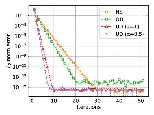
Figure 1: $L_{2}$ error $\lVert m_{n}-\theta_{ref}\rVert_{2}$ of the linear 2-parameter model problem. NS: non-singular system, OD: over-determined system, UD: under-determined system.

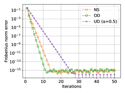
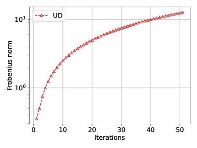
Figure 2: Frobenius norm $\lVert C_{n}-C_{\infty}\rVert_{F}$ (left) for non-singular (NS) and over-determined (OD) systems, and $\lVert C_{n}\rVert_{F}$ (right) for the under-determined (UD) system of the linear 2-parameter model problem.

5.4 Hilbert Matrix Problem

In this example $N_{y}=N_{\theta}.$ We define the Hilbert matrix $G\in R^{N_{\theta}\times N_{\theta}}$ by its entries

$$G_{i,j}=\frac{1}{i+j-1}.$$

The condition number of $G$ grows as $\mathcal{O}\Big{(}(1+\sqrt{2})^{4N_{\theta}}/\sqrt{N_{\theta}}\Big{)}$ [92]. We consider the inverse problem of finding $\theta\in\mathbb{R}^{N_{\theta}}$ from $y\in\mathbb{R}^{N_{y}}$ where $y=G\theta_{ref}$ and we define $\theta_{ref}:=\mathds{1}.$ The ill-conditioning of $G$ makes the determination of $\theta$ from $y$ difficult. Traditional linear solvers fail for such a problem.

We consider two scenarios: $N_{\theta}=10$ and $N_{\theta}=100$. As in the previous linear case study we assume a model misspecification setting in which $\Sigma_{\eta}=0.1^{2}\mathbb{I}$, even though the data itself contains no noise, and we take $\alpha=1.$ We set $r_{0}=0$ and $\gamma=0.5^{2}$. Thus $\theta_{0}\sim\mathcal{N}(0,0.5^{2}\mathbb{I})$. Both UKI and EKI are applied. For the EKI, the ensemble sizes are set to $J=2N_{\theta}+1$ and $J=100N_{\theta}+1$. The convergence of the parameter vector $m_{n}$ is depicted in Fig. 3. The UKI converges, but the convergence rate depends on the condition number of $G$, slowing as it grows. The EKI converges to a certain accuracy as fast as the UKI and then diverges. This divergence is related to the finite ensemble size, and is delayed by use of the larger $J$. Indeed in the mean-field limit $J=\infty$ the EKI will coincide with the UKI. This example clearly demonstrates the benefits of the UKI over the EKI.

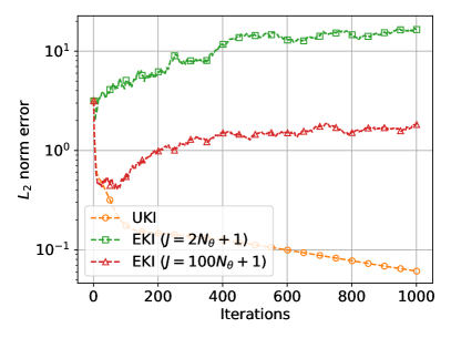
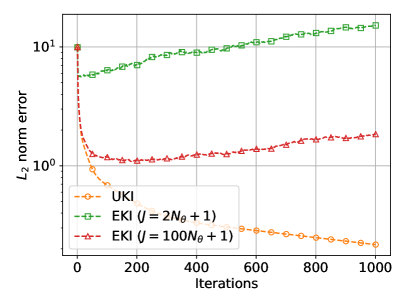
Figure 3: $L_{2}$ error $\lVert m_{n}-\theta_{ref}\rVert_{2}$ of the Hilbert inverse problem with $N_{\theta}=10$ (left) and $N_{\theta}=100$ (right).

5.5 Darcy Flow Problem

Consider the Darcy flow equation on the two-dimensional spatial domain $D=[0,1]^{2}$. The forward model is to find the pressure field $p(x)$ in a porous medium defined by a positive permeability field $a(x,\theta)$:

$$-\nabla\cdot(a(x,\theta)\nabla p(x)) =f(x),\quad x\in D,$$

$$p(x) =0,\quad x\in\partial D.$$

For simplicity, we have imposed homogeneous Dirichlet boundary conditions on the pressure at the boundary $\partial D$. The fluid source field $f$ is defined as

$$f(x_{1},x_{2})=\begin{cases}1000&0\leq x_{2}\leq\frac{4}{6}\\ 2000&\frac{4}{6}<x_{2}\leq\frac{5}{6}\\ 3000&\frac{5}{6}<x_{2}\leq 1\\ \end{cases}.$$

We study the inverse problems of finding $a$ from noisy measurements of $p$. We place a prior on the permeability field $a(x,\theta)$ by assuming that $\log a(x,\theta)$ is a centred Gaussian with covariance

$$\mathsf{C}=(-\Delta+\tau^{2})^{-d};$$

here $-\Delta$ denotes the Laplacian on $D$ subject to homogeneous Neumann boundary conditions on the space of spatial-mean zero functions, $\tau>0$ denotes the inverse length scale of the random field and $d>0$ determines its regularity ($\tau=3$ and $d=2$ in the present study). See [4, 93, 6, 94] for examples. The parameter $\theta$ represents the countable set of coefficients in the Karhunen-Loève (KL) expansion of the Gaussian random field:

$$\log a(x,\theta)=\sum_{l\in K}\theta_{(l)}\sqrt{\lambda_{l}}\psi_{l}(x),$$ (49)

where $K=\mathbb{Z}^{0+}\times\mathbb{Z}^{0+}\setminus\{0,0\}$, $\theta_{(l)}\sim\mathcal{N}(0,1)$ i.i.d. and the eigenpairs are of the form

$$\psi_{l}(x)=\begin{cases}\sqrt{2}\cos(\pi l_{1}x_{1})&l_{2}=0\\ \sqrt{2}\cos(\pi l_{2}x_{2})&l_{1}=0\\ 2\cos(\pi l_{1}x_{1})\cos(\pi l_{2}x_{2})&\textrm{otherwise}\\ \end{cases},\qquad\lambda_{l}=(\pi^{2}|l|^{2}+\tau^{2})^{-d}.$$

The KL expansion equation 49 can be rewritten as a sum over $\mathbb{Z}^{0+}$ rather than a lattice:

$$\log a(x,\theta)=\sum_{k\in\mathbb{Z}^{0+}}\theta_{(k)}\sqrt{\lambda_{k}}\psi_{k}(x),$$ (50)

where the eigenvalues $\lambda_{k}$ are in descending order. In practice, we truncate this sum to $N_{\theta}$ terms, based on the largest $N_{\theta}$ eigenvalues, and hence $\theta\in\mathbb{R}^{N_{\theta}}$. The forward problem is solved by a finite difference method on an $80\times 80$ grid.

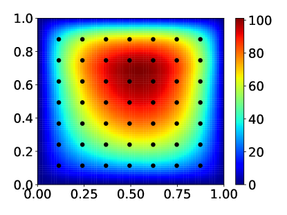
Figure 4: The pressure field of the Darcy flow problem and the $49$ equidistant pointwise measurements (black dots).

For the inverse problem, the observation $y_{ref}$ consists of pointwise measurements of the pressure value $p(x)$ at $49$ equidistant points in the domain (See Fig. 4). We generate a truth random field $\log a_{{ref}}(x)$ with $\theta\sim\mathcal{N}(0,\mathbb{I})$ in $\mathbb{R}^{256}$ (i.e. we use the first $256$ KL modes) to construct the observation $y_{ref}$; different levels of noise are added to make data $y_{obs}$ as explained in (48). Using this data, we consider two incomplete parameterization scenarios: solving for the first $32$ KL modes ($N_{\theta}=32$) and for the first $8$ KL modes ($N_{\theta}=8$). EKI and UKI are both applied. We take $r_{0}=0$ and $\gamma=1$ so that $\theta_{0}\sim\mathcal{N}(0,\mathbb{I})$. The observation error satisfies $\eta\sim\mathcal{N}(0,\mathbb{I})$. For the EKI, the ensemble size is set to be $J=100$, which is larger than the number of $\sigma-$points used in UKI ($2N_{\theta}+1$).

For the $N_{\theta}=32$ case, the convergence of the log-permeability fields $\log a(x,m_{n})$ and the optimization errors (3) at each iteration for different noise levels are depicted in Fig. 5; the top row shows the relative $L_{2}$ errors in the estimate of $\log a$ and the bottom row shows the optimization errors (data-misfit), left to right corresponds to different noise levels in the data. Without explicit regularization ($\alpha=1.0$), both UKI and EKI suffer from overfitting for noisy scenarios: the optimization errors keep decreasing, but the parameter errors show the “U-shape” characteristic of overfitting. Adding regularization ($\alpha=0.5$) relieves the overfitting. The estimated log-permeability fields $\log a(x,m_{n})$ at the 50th iteration and the truth random field are depicted in Fig. 6. Both UKI and EKI deliver similar results and these estimated log-permeability fields capture main features of the truth random field.

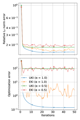
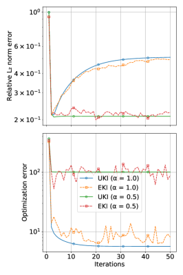
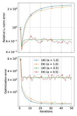
Figure 5: Relative error $\displaystyle\frac{\lVert\log a(x,m_{n})-\log a_{ref}(x)\rVert_{2}}{\lVert\log a_{ref}(x)\rVert_{2}}$ (top) and the optimization error $\displaystyle\frac{1}{2}\lVert\Sigma_{\eta}^{-\frac{1}{2}}(y_{obs}-\widehat{y}_{n})\rVert^{2}$ (bottom) of the Darcy problem ($N_{\theta}=32$) with different noise levels: noiseless (left), $1\%$ error (middle), and $5\%$ error (right).

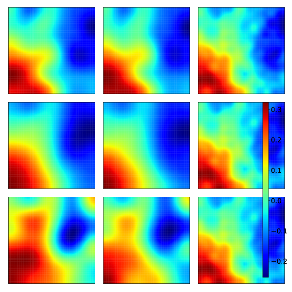
Figure 6: Log-permeability fields $\log a(x,m_{n})$ with $N_{\theta}=32$ obtained by UKI, EKI, and the truth (left to right) for different noise levels: noiseless $\alpha=1$ (top), $1\%$ noise $\alpha=0.5$ (middle), $5\%$ noise $\alpha=0.5$ (bottom).

For the $N_{\theta}=8$ case, the convergence of the log-permeability fields $\log a(x,m_{n})$ and the optimization errors at each iteration for different noise levels are depicted in Fig. 7. Even without explicit regularization ($\alpha=1.0$), none of these Kalman inversions suffer from overfitting. Both UKI and EKI lead to similar parameter errors and optimization errors. The estimated log-permeability fields $\log a(x,m_{n})$ at the 50th iteration for different noise levels, obtained by the UKI and the truth random field, are depicted in Fig. 8. Comparing with the $N_{\theta}=32$ case, all Kalman inversions with $N_{\theta}=8$ perform better for the $5\%$ noise scenario. This indicates the possibility of regularizing the inverse problem by reducing the parameter dimensionality.

Finally we observe the smoothness, as a function of the iteration number, of the UKI in comparison to EKI. This may be seen in all the experiments undertaken in the Darcy flow example.

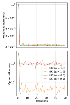
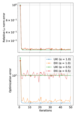
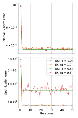
Figure 7: Relative error $\displaystyle\frac{\lVert\log a(x,m_{n})-\log a_{ref}(x)\rVert_{2}}{\lVert\log a_{ref}(x)\rVert_{2}}$ (top) and the optimization error $\displaystyle\frac{1}{2}\lVert\Sigma_{\eta}^{-\frac{1}{2}}(y_{obs}-\widehat{y}_{n})\rVert^{2}$ (bottom) of the Darcy problem ($N_{\theta}=8$) with different noise levels: noiseless (left), $1\%$ error (middle), and $5\%$ error (right).

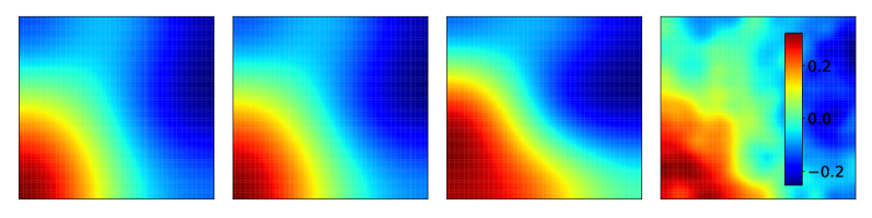
Figure 8: Log-permeability fields $\log a(x,m_{n})$ with $N_{\theta}=8$ obtained by the UKI and the truth (right) for different noise levels: noiseless $\alpha=1$ (left), $1\%$ noise $\alpha=1$ (middle-left), $5\%$ noise $\alpha=1$ (middle-right).

5.6 Damage Detection Problem

Consider a thin linear elastic arch-like plate, which is fixed on the bottom edges $\Gamma_{u}$. A traction boundary condition is applied on the top edge $\Gamma_{t_{1}}$, with distributed load $\bar{t}=(2,-20)$, and a traction free boundary condition is applied on the remaining edges $\Gamma_{t_{2}}$. See Fig. 9 The equations of linear elastostatics with plane stress assumptions are expressed in terms of the (Cauchy) stress tensor $\sigma$ and take the form

$$\begin{split}\nabla\cdot\sigma+b&=0\textrm{ in }\Omega,\\ u&=0\textrm{ on }\Gamma_{u},\\ \sigma\cdot n&=\bar{t}\textrm{ on }\Gamma_{t_{1}},\\ \sigma\cdot n&=0\textrm{ on }\Gamma_{t_{2}}.\end{split}$$ (51)

Here $u$ is the displacement vector, $b=0$ is the body force vector, $\Omega\in\mathbb{R}^{2}$ is the bounded domain occupied by the plate. The strain tensor is

$$\varepsilon_{mn}=\frac{1}{2}\Big{(}\frac{\partial u_{n}}{\partial x_{m}}+\frac{\partial u_{m}}{\partial x_{n}}\Big{)}.$$ (52)

The linear constitutive relation between strain and stress is written as

$$\sigma_{ij}=\mathsf{C}_{ijmn}(E,\nu)\varepsilon_{mn}.$$ (53)

Here $\mathsf{C}_{ijmn}$ are the constitutive tensor components, which depend on the Young’s modulus $E$ and Poisson’s ratio $\nu$; throughout this study, we fix $\nu=0.4$ and focus on learning the spatially-dependent damage information present in the field $E.$ The damage is assumed to be isotropic elasticity-based damage with

$$E(x,\theta)=\big{(}1-\omega(x,\theta)\big{)}E_{0}.$$

Throughout this study, we fix $E_{0}=1000$, and $\omega(x,\theta)$ is the scalar-valued damage variable, which varies between zero (no damage) to one (complete damage). The truth damage field (See Fig. 9-left) is

$$\begin{split}&\omega_{ref}(x)=a_{1}e^{-\frac{1}{2}(x-x_{1})\Sigma^{-1}_{1}(x-x_{1})}+a_{2}e^{-\frac{1}{2}(x-x_{2})\Sigma^{-1}_{2}(x-x_{2})}+a_{3}e^{-\frac{1}{2}(x-x_{3})\Sigma^{-1}_{3}(x-x_{3})},\\ &a_{1}=0.8,\,a_{2}=0.6,\,a_{3}=0.5,\,\\ &x_{1}=\begin{bmatrix}50\\ 50\end{bmatrix},\,x_{2}=\begin{bmatrix}250\\ 160\end{bmatrix},\,x_{3}=\begin{bmatrix}380\\ 100\end{bmatrix},\,\Sigma_{1}=\begin{bmatrix}200&0\\ 0&200\end{bmatrix},\,\Sigma_{2}=\begin{bmatrix}800&0\\ 0&400\end{bmatrix},\,\Sigma_{3}=\begin{bmatrix}100&0\\ 0&400\end{bmatrix},\,\end{split}$$

and may be seen to exhibit three flaws. Noise is added to the observations on the boundary as in (48). The forward equation is solved by the finite element method with $384$ quadratic quadrilateral elements ($1649$ nodes) using the NNFEM library [39, 40].

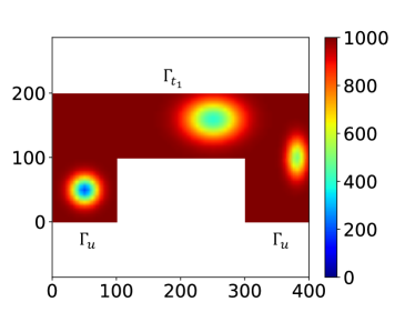
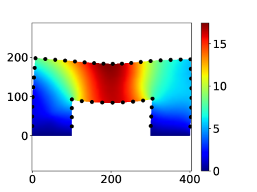
Figure 9: The damaged Young’s modulus (left) and the displacement magnitude field (right) with $46$ measurement locations on the surface of the boundaries (black dots). The five unlabelled edges comprise $\Gamma_{t_{2}}$; see equation (51).

For the inverse problem, the damage field is parameterized in terms of field $\theta(x)$ as follows

$$\omega(\theta(x))=0.9\frac{1-e^{-\theta(x)}}{1+9e^{-\theta(x)}}\in(-0.1,0.9).$$

Field $\theta(x)$ is itself discretized and represented by 24 quadratic quadrilateral elements ($N_{\theta}=125$). The observations are $x_{1}$ and $x_{2}$ displacements measured at 46 ($N_{y}=92$) locations on the surface boundaries (see Fig. 9-right). We consider both $\alpha=0.5$ and $\alpha=1.0$, and we set $r_{0}=0$ and $\gamma=1.$ The UKI and EKI are both applied, initialized with $\theta_{0}\sim\mathcal{N}(0,\mathbb{I})$. The observation error model used in the algorithm is $\eta\sim\mathcal{N}(0,0.1^{2}\mathbb{I})$. For this problem the prior information $\omega(\theta=0)=0$ corresponds to an undamaged plate, and is expected to be reasonable for most of the domain. For the EKI, the ensemble size is set to $J=500$, which is larger than the number of $\sigma-$points used in UKI ($2N_{\theta}+1$).

The convergence of the damage field $\omega(\theta(x,m_{n}))$ and the optimization errors at each iteration are depicted in Fig. 10; the organization of the information is the same as in the Darcy flow example. In the noiseless scenario, the EKI exhibits divergence without regularization ($\alpha=1.0$) due to the ill-posedness, however, the UKI converges . For noisy scenarios, the effect of overfitting is significant. At $1\%$ noise level, setting $\alpha=0.5$ eliminates overfitting; however at $5\%$ noise level, setting $\alpha=0.5$ does not eliminate overfitting. Therefore, the results obtained with $\alpha=0.0$ are also reported for the $5\%$ noise scenario. The estimated damaged Young’s modulus fields $E(x,\theta)$ and the truth are depicted in Fig. 11. Both Kalman inversion methods perform comparably, and these three flaw areas are captured; however at $5\%$ noise level noticeable bias is visible in the flaws to the left and right of the domain. As in the Darcy flow case, the convergence histories of the UKI are smoother than for the EKI.

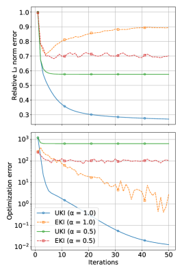
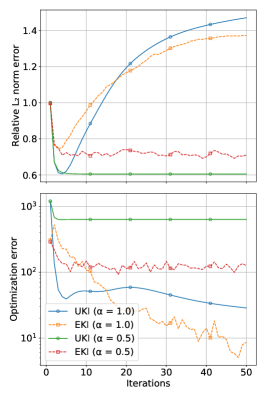
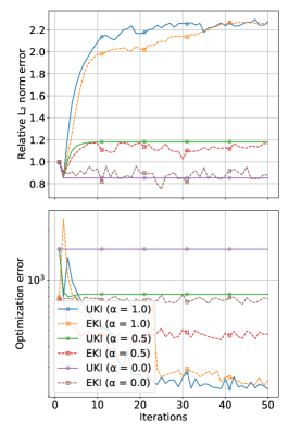
Figure 10: Relative error $\displaystyle\frac{\lVert\omega(\theta(x,m_{n}))-\omega_{ref}\rVert_{2}}{\lVert\omega_{ref}\rVert_{2}}$ (top) and the optimization error $\displaystyle\frac{1}{2}\lVert\Sigma_{\eta}^{-\frac{1}{2}}(y_{obs}-\widehat{y}_{n})\rVert^{2}$ (bottom) of the damage detection problem with different noise levels: noiseless (left), $1\%$ error (middle), and $5\%$ error (right).

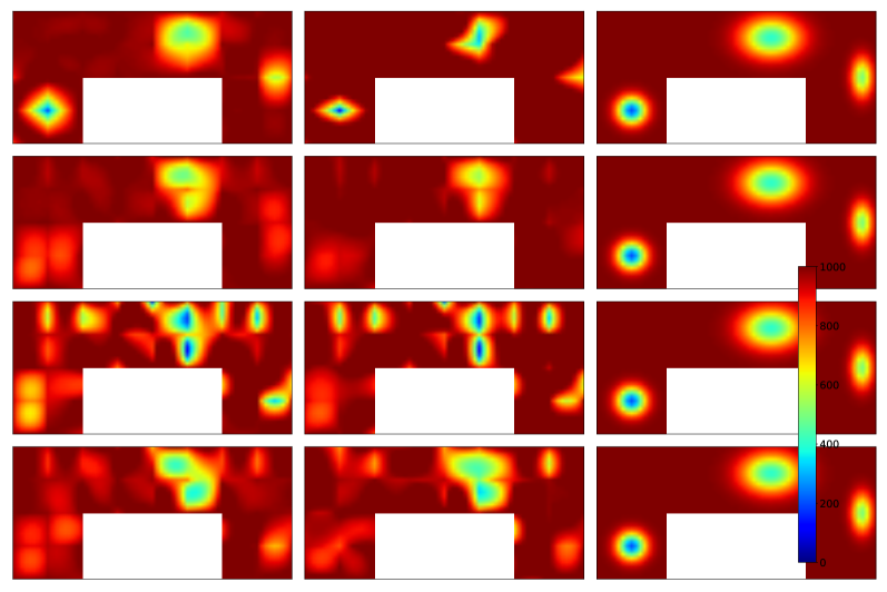
Figure 11: Damaged Young’s modulus fields $(1-\omega(x,m_{n}))E_{0}$ obtained by UKI, EKI, and the truth (left to right) at different noise levels: noiseless $\alpha=1$, $1\%$ noise $\alpha=0.5$, $5\%$ noise $\alpha=0.5$, and $5\%$ noise $\alpha=0$ (top to bottom).

5.7 Navier-Stokes Problem

We consider the 2D Navier-Stokes equation on a periodic domain $D=[0,2\pi]\times[0,2\pi]$:

$$\begin{split}&\frac{\partial v}{\partial t}+(v\cdot\nabla)v+\nabla p-\nu\Delta v=0,\\ &\nabla\cdot v=0,\\ \end{split}$$

with initial condition chosen to imply the conservation law

$$\frac{1}{4\pi^{2}}\int v=v_{b}.$$

Here $v$ and $p$ denote the velocity vector and the pressure, $\nu=0.01$ denotes the dynamic viscosity, and $v_{b}=(2\pi,2\pi)$ denotes the non-zero mean background velocity. The forward problem is rewritten in the vorticity-streamfunction ($\omega-\psi$) formulation:

$$\begin{split}&\frac{\partial\omega}{\partial t}+(v\cdot\nabla)\omega-\nu\Delta\omega=0,\\ &\omega=-\Delta\psi\qquad\frac{1}{4\pi^{2}}\int\psi=0,\\ &v=\Big{(}\frac{\partial\psi}{\partial x_{2}},-\frac{\partial\psi}{\partial x_{1}}\Big{)}+v_{b},\end{split}$$

and solved by the pseudo-spectral method [95] on a $128\times 128$ grid. To eliminate aliasing error, the Orszag 2/3-Rule [96] is applied and, therefore there are $85^{2}$ Fourier modes (padding with zeros). Time-integration is performed using the Crank–Nicolson method with $\Delta T=2.5\times 10^{-4}$.

We study the problem of recovering the initial vorticity field from measurements at positive times. We parameterize this field as $\omega_{0}(x,\theta)$, defined by parameters $\theta\in\mathbb{R}^{N_{\theta}}$, and modeled a priori as a Gaussian field with covariance operator $\mathsf{C}=\Delta^{-2}$, subject to periodic boundary conditions, on the space of spatial-mean zero functions. The KL expansion of the initial vorticity field is given by

$$\omega_{0}(x,\theta)=\sum_{l\in K}\theta^{c}_{(l)}\sqrt{\lambda_{l}}\psi^{c}_{l}+\theta^{s}_{(l)}\sqrt{\lambda_{l}}\psi^{s}_{l},$$ (54)

where $K=\{(k_{x},k_{y})|k_{x}+k_{y}>0\textrm{ or }(k_{x}+k_{y}=0\textrm{ and }k_{x}>0)\}$, and the eigenpairs are of the form

$$\psi^{c}_{l}(x)=\frac{\cos(l\cdot x)}{\sqrt{2}\pi}\quad\psi^{s}_{l}(x)=\frac{\sin(l\cdot x)}{\sqrt{2}\pi}\quad\lambda_{l}=\frac{1}{|l|^{4}},$$

and $\theta^{c}_{(l)},\theta^{s}_{(l)}\sim\mathcal{N}(0,2\pi^{2})$ i.i.d. The KL expansion equation 54 can be rewritten as a sum over $\mathbb{Z}^{0+}$ rather than a lattice:

$$\omega_{0}(x,\theta)=\sum_{k\in\mathbb{Z}^{0+}}\theta_{(k)}\sqrt{\lambda_{k}}\psi_{k}(x),$$ (55)

where the eigenvalues $\lambda_{k}$ are in descending order.

For the inverse problem, we recover the initial condition, specifically the initial vorticity field of the Navier-Stokes equation, given pointwise observations $y_{ref}$ of the vorticity field at 16 equidistant points ($N_{y}=32$) at $T=0.25$ and $T=0.5$ (See Fig. 12). The observations $y_{obs}$ are defined as in (48). The initial vorticity field $\omega_{0,ref}$ is generated with all $85^{2}$ Fourier modes, and the first $N_{\theta}=100$ KL modes of equation 55 are recovered. We take $\alpha=1.0$ and $\alpha=0.9$, and fix $r_{0}=0$ and $\gamma=10$. Both UKI and EKI are applied with $\theta_{0}\sim\mathcal{N}(0,10\mathbb{I})$ and the observation error assumed for inversion purposes is $\eta\sim\mathcal{N}(0,\mathbb{I})$. For the EKI, the ensemble size is set to be $J=201$, which equals the number of $\sigma-$points in UKI ($2N_{\theta}+1$).

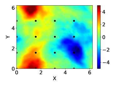
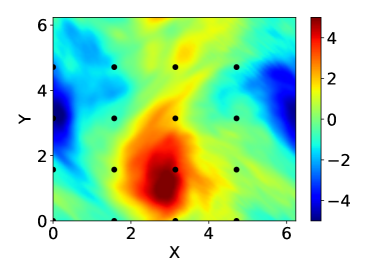
Figure 12: The vorticity fields of the Navier-Stokes problem and the $16$ equidistant pointwise measurements (black dots) at two observation times ($T=0.25$ and $T=0.5$).

The convergence of the initial vorticity field $\omega_{0}(x,m_{n})$ and the optimization errors for different noise levels at each iteration are depicted in Fig. 13; the organization of the figure is the same as in the Darcy case. In all scenarios, the UKI outperforms EKI. Moreover, without regularization ($\alpha=1.0$), EKI exhibits slight divergence. This inverse problem is not sensitive to added Gaussian random noise, and the behavior of any given Kalman inversion, with respect to different noise levels, are almost indistinguishable. The estimated initial vorticity fields $\omega_{0}(x,m_{n})$ at the 50th iteration for different noise levels obtained by the Kalman inversions and the truth random field are depicted in Fig. 14. Both Kalman inversions capture main features of the truth random initial field, but not the detailed small features, due to the irreversibility of the diffusion process ($\nu=0.01$).

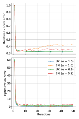
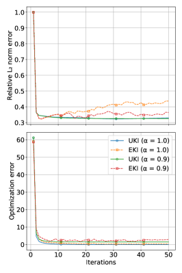
Figure 13: Relative error $\frac{\lVert\omega_{0}(x,m_{n})-\omega_{0,ref}\rVert_{2}}{\lVert\omega_{0,ref}\rVert_{2}}$ (top) and the optimization error $\displaystyle\frac{1}{2}\lVert\Sigma_{\eta}^{-\frac{1}{2}}(y_{obs}-\widehat{y}_{n})\rVert^{2}$ (bottom) of the Navier-Stokes problem with different noise levels: noiseless (left), $1\%$ error (middle), and $5\%$ error (right).

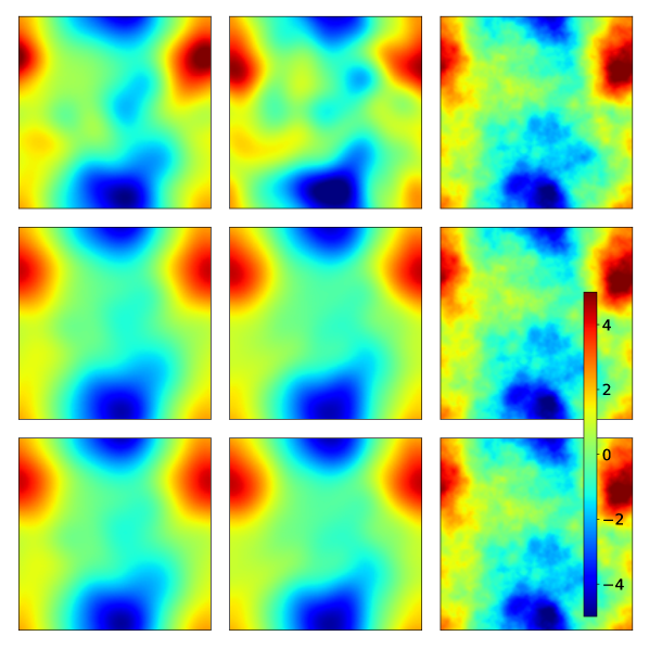
Figure 14: Initial vorticity fields $\omega_{0}(x,m_{n})$ recovered by UKI, EKI, and the truth (left to right) for different noise levels: noiseless $\alpha=1$, $1\%$ noise $\alpha=0.9$, $5\%$ noise $\alpha=0.9$ (top to bottom).

5.8 Lorenz63 Model Problem

Consider the Lorenz63 system, a simplified mathematical model for atmospheric convection [97]:

$$\begin{split}&\frac{dx_{1}}{dt}=\sigma(x_{2}-x_{1}),\\ &\frac{dx_{2}}{dt}=x_{1}(r-x_{3})-x_{2},\\ &\frac{dx_{3}}{dt}=x_{1}x_{2}-\beta x_{3};\\ \end{split}$$

the system is parameterized by $\sigma,r,\beta\in\mathbb{R}_{+}$. We consider learning various subsets of these parameters from time-averaged data. To be concrete, the observation consists of the time-average of the various moments over time windows of size $T=20$, with an initial spin-up period $T=30$ to eliminate the influence of the initial condition; if $f:\mathbb{R}^{3}\mapsto\mathbb{R}$ computes a moment, then we define

$$\overline{f(x)}=\frac{1}{20}\int_{30}^{50}f\bigl{(}x(t)\bigr{)}dt.$$ (56)

We view this as an approximation of the ergodic average

$$\mathbb{E}f(x)=\lim_{\tau\to\infty}\frac{1}{\tau}\int_{0}^{\tau}f\bigl{(}x(t)\bigr{)}dt.$$

If the observation operator comprises finite time averages of the form (56) for a collection of moments $f(x)$ then we may reformulate the inverse problem as

$$y=\mathcal{G}(r)+\eta$$ (57)

with $\eta$ a Gaussian which may be estimated from a long time trajectory (we use $T=200$) by appealing to the central limit theorem [98]. In this interpretation $\mathcal{G}$ is the ergodic average. Note, however, that when we run any algorithm we will only use finite-time average approximations of $\mathcal{G}$.

The truth observation is computed with parameters $(\sigma,\ r,\ \beta)=(10,\ 28,\ 8/3)$ over a time window of size $T=200$, also with an initial spin-up period $T=30$. To estimate the statistics of $\eta$ we split the observation time-series into $10$ windows of size $T=20$ and compute covariance of the observation error $\eta$ following [62]. We set $r_{0}=5.0\mathds{1}$ and $\gamma=1$. The UKI is initialized with $\theta_{0}\sim\mathcal{N}(5.0\mathds{1},\mathbb{I})$, and $\alpha$ is set to $1.$

We start with the following one-parameter inverse problem with fixed $\sigma=10$ and $\beta=8/3$:

$$y=\mathcal{G}(r)+\eta\quad\mathrm{with}\quad y=\overline{x_{3}}.$$ (58)

The UKI is applied, and the estimated $r$ and the associated 3-$\sigma$ confidence intervals at each iteration are depicted in Fig. 15. The confidence intervals give an indication of the evolving covariance $C_{n}$. The estimation of $r$ at the 20th iteration is $r\sim\mathcal{N}(28.03,0.22)$.

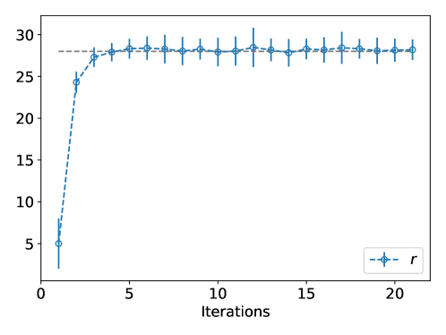
Figure 15: Convergence of the 1-parameter Lorenz63 inverse problem with UKI ($\alpha=1.0$); the true parameter value is represented by the dashed grey line.

The landscape of $\mathcal{G}$ and sensitivity of $\mathcal{G}(\cdot)$ with respect to the input for observations, derived from chaotic problems such as equation 58, are widely studied [63, 64]. We study them further, here, and the results are depicted in Fig. 16. The function $\mathcal{G}$ is characterized by a sudden change at $r\approx 22$ and the landscape is highly oscillatory for $r>22$; furthermore, the sensitivity $d\mathcal{G}(r)$ computed with the discrete adjoint method blows up:

$$|d\mathcal{G}(r)|\propto\mathcal{O}(e^{\lambda T}),$$

with the value of the exponent $\lambda$ consistent with the first global Lyapunov exponent [63, 99]. This illustrates the challenges inherent in parameter estimation and sensitivity analyses for chaotic systems. In particular, the ExKI method suffers from the large derivatives of $\mathcal{G}$. Based on Lemma 2, it is natural to study the landscape of the averaged function $\mathcal{F}\mathcal{G}$ and its associated gradient $\mathcal{F}d\mathcal{G}$, with the standard deviation $\sigma_{r}=\sqrt{0.22}$ fixed; this gives an indication of the landscape as perceived by the UKI. In particular, we have:

$$\begin{split}\mathcal{F}\mathcal{G}(r)=\int\mathcal{G}(x)\frac{1}{\sqrt{2\pi}\sigma_{r}}e^{-\frac{(x-r)^{2}}{2\sigma_{r}^{2}}}dx,\qquad\mathcal{F}d\mathcal{G}(r)=\frac{\int(x-r)(\mathcal{G}(x)-\mathcal{G}(r))\frac{1}{\sqrt{2\pi}\sigma_{r}}e^{-\frac{(x-r)^{2}}{2\sigma_{r}^{2}}}dx}{\int(x-r)^{2}\frac{1}{\sqrt{2\pi}\sigma_{r}}e^{-\frac{(x-r)^{2}}{2\sigma_{r}^{2}}}dx}.\end{split}$$

These functions are depicted in Fig. 17, which should be compared with Fig. 16. We see that $\mathcal{F}\mathcal{G}$ is smooth (except the transition point), and $\mathcal{F}d\mathcal{G}$ does not suffer from blow-up in the way $d\mathcal{G}$ does; furthermore, $\mathcal{F}d\mathcal{G}$ represents the averaged gradient $\overline{d\mathcal{G}(r)}\approx 0.96$ well, away from the blow-up regions. This explains why the adjoint/gradient-based methods, including ExKI, fail, but the UKI succeeds for this chaotic inverse problem.

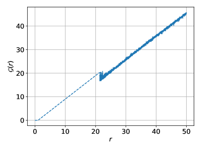
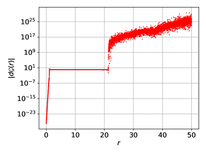
Figure 16: Landscape (left) and sensitivity (right) of $\mathcal{G}$ in the 1-parameter Lorenz63 inverse problem equation 58

Figure 17: Landscape (left) and sensitivity (right) of $\mathcal{F}\mathcal{G}$ in the 1-parameter Lorenz63 inverse problem equation 58 smoothed and viewed by UKI.

Next, we consider a three-parameter inverse problem, using the ideas in Subsection 4.1. Let $\theta=(\theta_{(1)},\theta_{(2)},\theta_{(3)})$ and let $(\sigma,r,\beta)=(|\theta_{(1)}|,|\theta_{(2)}|,|\theta_{(3)}|).$ The map $\mathcal{G}(\theta)$ is found by computing time-averages of all three components of $x$, as described above, for given input parameter $\theta.$ The use of the modulus helps ensure solution trajectories which do not blow-up. We have

$$y=\mathcal{G}(\theta)+\eta\quad\mathrm{with}\quad y=(\overline{x_{1}},\overline{x_{2}},\overline{x_{3}},\overline{x_{1}^{2}},\overline{x_{2}^{2}},\overline{x_{3}^{2}}).$$ (59)

All other aspects of the setup are the same as the aforementioned one-parameter inverse problem. The estimated parameters and associated 3-$\sigma$ confidence intervals for each component at each iteration are depicted in Fig. 18. The estimation of the parameters at the 20th iteration is

$$\left(\sigma\quad r\quad\beta\right)=\left(10.28\quad 27.90\quad 2.63\right)$$

For both scenarios, the UKI converges efficiently, thanks to the linear (or superlinear) convergence rate of the LMA and the averaging property.

Figure 18: Convergence of the 3-parameter Lorenz63 inverse problem with UKI ($\alpha=1.0$); true parameter values are represented by dashed grey lines.

5.9 Multiscale Lorenz96 Problem

Consider the multi-scale Lorenz96 system, a simplified mathematical model for the midlatitude atmosphere [100], with $K$ slow variables $X^{(k)}$ which are each coupled with $J$ fast variables $Y^{(j,k)}$, given by:

$$\begin{split}&\frac{dX^{(k)}}{dt}=-X^{(k-1)}(X^{(k-2)}-X^{(k+1)})-X^{(k)}+F-\frac{hc}{b}\sum_{j=1}^{J}Y^{(j,k)},\\ &\frac{dY^{(j,k)}}{dt}=-cbY^{(j+1,k)}(Y^{(j+2,k)}-Y^{(j-1,k)})-cY^{(j,k)}+\frac{hc}{b}X^{k}.\end{split}$$ (60)

To close the system, it is appended with the cyclic boundary conditions $X^{(k+K)}=X^{(k)}$, $Y^{(j,k+K)}=Y^{(j,k)}$ and $Y^{(j+J,k)}=Y^{(j,k+1)}$. The time scale separation is parameterized by the coefficient $c$ and the large-scales are subjected to external forcing $F$. We choose here as parameters $K=8$, $J=32$, $F=20$, $c=b=10$ and $h=1$ as in [101, 102, 103, 104]. As time-integrator, we use the 4th-order Runge Kutta method with $\Delta T=5\times 10^{-3}$.

Our goal is to learn the closure model $\psi(X)$ of the fast dynamics for a reduced model of the form

$$\frac{dX^{(k)}}{dt}=-X^{(k-1)}(X^{(k-2)}-X^{(k+1)})-X^{(k)}+F+\psi(X^{(k)}).$$

The closure model $\psi:D\subset\mathbb{R}\mapsto\mathbb{R}$ is parameterized by the finite element method with cubic Hermite polynomials. The domain is set to be $D=[-20,20]$ and decomposed into $5$ elements and, therefore, $N_{\theta}=12$.

For the inverse problem, the observations consist of the time-average of the first and second moments of $X^{(1)},X^{(2)},X^{(3)}$, and $X^{(4)}$ over a time window of size $T=1000$ and, therefore $N_{y}=14$. The same central limit theorem arguments are used to formulate the problem as in the Lorenz63 model. The truth observation $y_{ref}$ is computed with the multiscale chaotic system equation 60 with a random initial condition $X^{(k)}\sim\mathcal{N}(0,1)\textrm{ and }Y^{(j,k)}\sim\mathcal{N}(0,0.01^{2})$. And $1\%$, $2\%$, and $5\%$ Gaussian random noises are added to the observation following equation 48.

We set $r_{0}=0$ and $\gamma=1$; the UKI is thus initialized with $\theta_{0}\sim\mathcal{N}(0,\mathbb{I})$. The observation error is set to be $\eta=\mathcal{N}(0,\textrm{diag}\{0.05^{2}y_{obs}\odot y_{obs}\})$, and we take $\alpha=1$, since the system is over-determined. Moreover, these simulations start with another random initialization of $X^{(k)}\sim\mathcal{N}(0,1)$. The learned closure models at the 20th iteration are reported in Fig. 19. The estimated empirical probability density functions of the slow variables are reported in Fig. 20. For all scenarios, although the learned closure models show non-trivial variability with respect to those published in [102, 103] at the left most extreme of $D$, the predicted probability density functions match well with the reference, obtained from a full multiscale simulation. It is worth mentioning this problem is not sensitive with respect to the added Gaussian random noise.

Figure 19: Closure terms $\psi(X)$ for the multi-scale Lorenz96 system obtained from the truth (grey dots) and polynomial data-fitting by Wilks [102] and Arnold [103], compared with what is learned using the UKI approach ($\alpha=1$) with different noise levels.

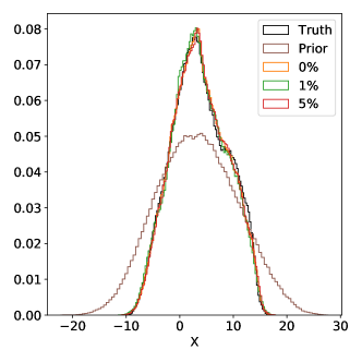
Figure 20: Empirical probability density functions of the slow variables $X^{(k)}$ obtained from the full multi-scale Lorenz96 system (Truth), the initial closure model (Prior), and the closure models learned by the UKI ($\alpha=1$) at different noise levels.

5.10 Idealized General Circulation Model

Finally, we consider an idealized general circulation model. The model is based on the 3D Navier-Stokes equations, making the hydrostatic and shallow-atmosphere approximations common in atmospheric modeling. Specifically, we test UKI on the well-known Held-Suarez test case [105], in which a detailed radiative transfer model is replaced by Newtonian relaxation of temperatures toward a prescribed “radiative equilibrium” $T_{\mathrm{eq}}(\phi,p)$ that varies with latitude $\phi$ and pressure $p$. Specifically, the thermodynamic equation for temperature $T$

$$\frac{\partial T}{\partial t}+\dots=Q$$

(dots denoting advective and pressure work terms) contains a diabatic heat source

$$Q=-k_{T}(\phi,p,p_{s})\bigl{(}T-T_{\mathrm{eq}}(\phi,p)\bigr{)},$$

with relaxation coefficient (inverse relaxation time)

$$k_{T}=k_{a}+(k_{s}-k_{a})\max\Bigl{(}0,\frac{\sigma-\sigma_{b}}{1-\sigma_{b}}\Bigr{)}\cos^{4}\phi.$$

Here, $\sigma=p/p_{s}$, which is pressure $p$ normalized by surface pressure $p_{s}$, is the vertical coordinate of the model, and

$$T_{\mathrm{eq}}=\max\Bigl{\{}200K,\Bigl{[}315K-\Delta T_{y}\sin^{2}\phi-\Delta\theta_{z}\log\Bigl{(}\frac{p}{p_{0}}\Bigr{)}\cos^{2}\phi\Bigr{]}\Bigl{(}\frac{p}{p_{0}}\Bigr{)}^{\kappa}\Bigr{\}}$$

is the equilibrium temperature profile ($p_{0}=10^{5}~{}\mathrm{Pa}$ is a reference surface pressure and $\kappa=2/7$ is the adiabatic exponent). Default parameters are

$$k_{a}=(40\ \mathrm{day})^{-1},\qquad k_{s}=(4\ \mathrm{day})^{-1},\qquad\Delta T_{y}=60\ \mathrm{K},\qquad\Delta\theta_{z}=10\ \mathrm{K}.$$

For the numerical simulations, we use the spectral transform method in the horizontal, with T42 spectral resolution (triangular truncation at wavenumber 42, with $64\times 128$ points on the latitude-longitude transform grid); we use 20 vertical levels equally spaced in $\sigma$. With the default parameters, the model produces an Earth-like zonal-mean circulation, albeit without moisture or precipitation. A single jet is generated with maximum strength of roughly $30\ \mathrm{m~{}s^{-1}}$ near $45^{\circ}$ latitude (Fig. 21).

Our inverse problem is constructed to learn parameters in the Newtonian relaxation term $Q$:

$$(k_{a},\ k_{s},\ \Delta T_{y},\ \Delta\theta_{z}).$$

We do so in the presence of the following constraints:

$$0\ \mathrm{day}^{-1}<k_{a}<1\ \mathrm{day}^{-1},\qquad k_{a}<k_{s}<1\ \mathrm{day}^{-1}+k_{a},\qquad 0\ \mathrm{K}<\Delta T_{y},\qquad 0\ \mathrm{K}<\Delta\theta_{z}.$$

Conceptually, the setting is identical to that for the Lorenz63 example. We use the same overline notation to denote averaging, which here in addition to the time average in the Lorenz models also includes a zonal average over longitude (because the model is statistically symmetric under rotations around the planet’s spin axis), and we apply the same central limit theorem arguments to formulate the inverse problem. To incorporate the imposition of the constraints, the inverse problem is formulated as follows (see Subsection 4.1 for details):

$$y=\mathcal{G}(\theta)+\eta\quad\mathrm{with}\quad\mathcal{G}(\theta)=\overline{T}(\phi,\sigma)$$ (61)

with the parameter transformation

$$\theta:(k_{a},k_{s},\Delta T_{y},\Delta\theta_{z})=\Big{(}\frac{1}{1+|\theta_{(1)}|},\ \frac{1}{1+|\theta_{(1)}|}+\frac{1}{1+|\theta_{(2)}|},\ |\theta_{(3)}|,|\theta_{(4)}|\Big{)}.$$ (62)

The observation mapping is defined by mapping from the unknown $\theta$ to the 200-day zonal mean of the temperature as a function of latitude ($\phi$) and height ($\sigma$), after an initial spin-up of 200 days. The truth observation is the 1000-day zonal mean of the temperature (see Fig. 21-a), after an initial spin-up 200 days to eliminate the influence of the initial condition. Because the truth observations come from an average 5 times as long as the observation window used for parameter learning, the chaotic internal variability of the model introduces noise in the observations. As for the Lorenz63 setting, the central limit theorem may be invoked to model the observation error from internal variability.

To perform the inversion, we set $r_{0}=[2\ \textrm{day},\ 2\ \textrm{day},\ 20\ \textrm{K},\ 20\ \textrm{K}]^{T}$ and $\gamma=1$. Thus UKI is initialized with $\displaystyle\theta_{0}\sim\mathcal{N}\Big{(}r_{0},\ \mathbb{I}\Big{)}.$ Within the algorithm, we assume that the observation error satisfies $\eta\sim\mathcal{N}(0\ \textrm{K},3^{2}\mathbb{I}\ \textrm{K}^{2})$. Because the problem is over-determined, we set $\alpha=1.$ The estimated parameters and associated 3-$\sigma$ confidence intervals for each component at each iteration are depicted in Fig. 22. The estimation of model parameters at the 20th iteration is

$$\left(k_{a}\quad k_{s}\quad\Delta T_{y}\quad\Delta\theta_{z}\right)=\left(0.0243\ \textrm{day}^{-1}\quad 0.243\ \textrm{day}^{-1}\quad 60.2\ \textrm{K}\quad 9.91\ \textrm{K}\right).$$

UKI converges to the true parameters in fewer than 10 iterations with 9 $\sigma$-points, demonstrating the potential of applying UKI for large-scale inverse problems.

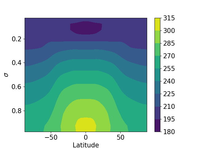
(a) T

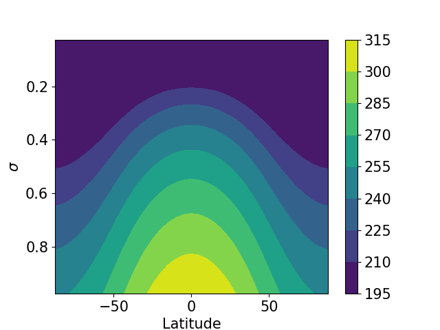
(b) T_eq

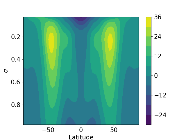
(c) U

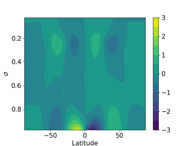
(d) V

Figure 21: Zonal mean profile of temperature (a), radiative equilibrium temperature (b), zonal wind velocity (c), and meridional wind velocity (d), all from a 1000-day average. The horizontal coordinate is latitude and the vertical coordinate is the nondimensional $\sigma$ coordinate of the model.

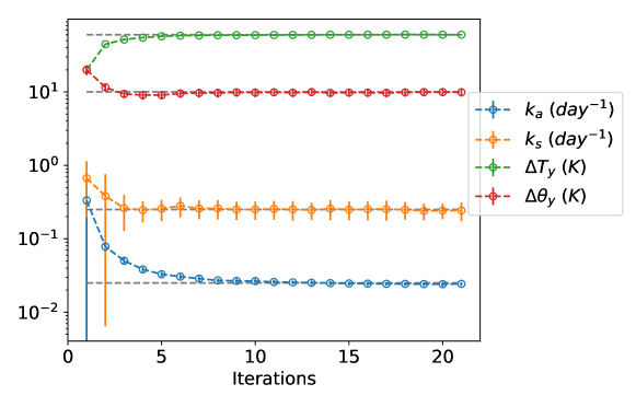
Figure 22: Convergence of the idealized general circulation model inverse problem with UKI ($\alpha=1.0$). The true parameter values are represented by dashed grey lines.

6 Conclusion

We introduced a novel stochastic dynamical system, into which an arbitrary inverse problem may be embedded as an observation operator; by applying filtering methods to this stochastic dynamical system we obtain methods to solve inverse problems. In the linear case, we have demonstrated that this approach leads to an unusual Tikhonov regularized least squares solution, with prior covariance depending on the forward model, and a tunable parameter in the stochastic dynamical system determining the level of regularization. We have also introduced unscented Kalman inversion (UKI) and shown that it outperforms the EKI, when applied to the same novel stochastic dynamical system. As well as outperforming EKI, UKI shares its advantages: it is derivative-free, black-box, embarrassingly parallel, and robust. Our numerical results demonstrate its theoretical properties and its applicability; in particular, it is demonstrated to outperform the EKI on large scale problems in which the number of unknown parameters is small. Because the methodology constitutes a novel approach to parameter estimation, there are many avenues for future research, including applications of the method, methodological improvements and extensions, and theoretical analysis.

Acknowledgments

This work was supported by the generosity of Eric and Wendy Schmidt by recommendation of the Schmidt Futures program and by the National Science Foundation (NSF, award AGS‐1835860). A.M.S. was also supported by the Office of Naval Research (award N00014-17-1-2079). The authors thank Sebastian Reich and anonymous reviewers for helpful comments on an earlier draft.

Appendix A Proof of Theorems

Proof of Proposition 1.

An affine transformation is an invertible mapping from $R^{N_{\theta}}$ to $R^{N_{\theta}}$ of the form ${}^{*}x=Ax+b$. When we apply the following affine transformation

$$\begin{split}&{}^{*}m_{n}=Am_{n}+b\qquad{}^{*}C_{n}=AC_{n}A^{T}\quad\textrm{ with }\quad{}^{*}r_{0}=Ar_{0}+b\qquad{}^{*}\Sigma_{\omega}=A\Sigma_{\omega}A^{T},\\ \end{split}$$

keep $y_{n}$ and $\Sigma_{\nu}$ unchanged, and define ${}^{*}\mathcal{G}(\theta)=\mathcal{G}\big{(}A^{-1}(\theta-b)\big{)}$. We prove

$${}^{*}m_{n+1}=Am_{n+1}+b\qquad{}^{*}C_{n+1}=AC_{n+1}A^{T}.$$ (63)

Equation 9 leads to

$${}^{*}\widehat{m}_{n+1}=\alpha{}^{*}m_{n}+(1-\alpha){}^{*}r_{0}=A\widehat{m}_{n+1}+b\qquad{}^{*}\widehat{C}_{n+1}=\alpha^{2}{}^{*}C_{n}+{}^{*}\Sigma_{\omega}=A\widehat{C}_{n+1}A^{T}.$$ (64)

Therefore, the distribution of ${}^{*}\theta_{n+1}|Y_{n}\sim\mathcal{N}({}^{*}\widehat{m}_{n+1}{}^{*}\widehat{C}_{n+1})$ is the same as $A\theta_{n+1}+b|Y_{n}$ and equation 10 becomes

$${}^{*}\widehat{y}_{n+1}=\widehat{y}_{n+1}\qquad{}^{*}\widehat{C}_{n+1}^{\theta y}=A\widehat{C}_{n+1}^{\theta y}\qquad{}^{*}\widehat{C}_{n+1}^{yy}=\widehat{C}_{n+1}^{yy}.$$ (65)

Finally, equation 11 leads to

$$\begin{split}{}^{*}m_{n+1}&={}^{*}\widehat{m}_{n+1}+{}^{*}\widehat{C}_{n+1}^{\theta y}({}^{*}\widehat{C}_{n+1}^{yy})^{-1}(y_{n+1}-{}^{*}\widehat{y}_{n+1})=Am_{n+1}+b,\\ {}^{*}C_{n+1}&={}^{*}\widehat{C}_{n+1}-{}^{*}\widehat{C}_{n+1}^{\theta y}({}^{*}\widehat{C}_{n+1}^{yy})^{-1}{{}^{*}\widehat{C}_{n+1}^{\theta y}}{}^{T}=AC_{n+1}A^{T}.\end{split}$$ (66)

∎

Proof of Lemma 1.

In this proof recall that $\theta\sim\mathcal{N}(m,C).$ When both $\mathcal{G}_{1}=G_{1}$ and $\mathcal{G}_{2}=G_{2}$ are linear transformations, we have

$$\mathbb{E}[\mathcal{G}_{i}(\theta)] =G_{i}\mathbb{E}[\theta]=G_{i}m=\mathcal{G}_{i}(m),$$

$$\mathrm{Cov}[\mathcal{G}_{1}(\theta),\mathcal{G}_{2}(\theta)] =G_{1}\mathrm{Cov}[\theta,\theta]G_{2}^{T}=G_{1}CG_{2}^{T},$$

$$\sum_{j=1}^{2N_{\theta}}W_{j}^{c}(\mathcal{G}_{1}(\theta^{j})-\mathbb{E}\mathcal{G}_{1}(\theta))(\mathcal{G}_{2}(\theta^{j})-\mathbb{E}\mathcal{G}_{2}(\theta))^{T} =\frac{1}{2a^{2}N_{\theta}}\sum_{j=1}^{2N_{\theta}}(G_{1}\cdot\theta^{j}-G_{1}m)(G_{2}\cdot\theta^{j}-G_{2}m)^{T}$$

$$=\frac{1}{2a^{2}N_{\theta}}\sum_{j=1}^{2N_{\theta}}2G_{1}c_{j}[\sqrt{C}]_{j}c_{j}[\sqrt{C}]_{j}G_{2}^{T}$$

$$=G_{1}CG_{2}^{T}.$$

In the following we use $\nabla^{k}\mathcal{G}_{i}$ to denote the $k^{th}$ derivative of $\mathcal{G}_{i}$ evaluated at $m$. For the nonlinear case, Taylor’s expansion of $\mathcal{G}_{i}(\cdot)$ at $m$ is then

$$\mathcal{G}_{i}(\theta)=\mathcal{G}_{i}(m)+\nabla\mathcal{G}_{i}\delta\theta+\frac{1}{2}\nabla^{2}\mathcal{G}_{i}\delta\theta\otimes\delta\theta+\frac{1}{6}\nabla^{3}\mathcal{G}_{i}\delta\theta\otimes\delta\theta\otimes\delta\theta+O(\|\delta\theta\|^{4})\quad\textrm{with}\quad\delta\theta=\theta-m.$$

The mean approximation is thus first-order accurate:

$$\mathbb{E}\mathcal{G}_{i}(\theta)=\mathcal{G}_{i}(m)+O(\|C\|).$$

The covariance approximation is second-order accurate:

$$\mathrm{Cov}[\mathcal{G}_{1}(\theta),\mathcal{G}_{2}(\theta)] =\mathbb{E}\left(\mathcal{G}_{1}(\theta)-\mathbb{E}\mathcal{G}_{1}(\theta)\right)\left(\mathcal{G}_{2}(\theta)-\mathbb{E}\mathcal{G}_{2}(\theta)\right)^{T}$$

$$=\mathbb{E}\left(\nabla\mathcal{G}_{1}\delta\theta+\frac{1}{2}\nabla^{2}\mathcal{G}_{1}(\delta\theta\otimes\delta\theta-C)\right)\left(\nabla\mathcal{G}_{2}\delta\theta+\frac{1}{2}\nabla^{2}\mathcal{G}_{2}(\delta\theta\otimes\delta\theta-C)\right)^{T}+\mathcal{O}(\|C\|^{2})$$

$$=\nabla\mathcal{G}_{1}C\nabla\mathcal{G}_{2}^{T}+\mathcal{O}(\|C\|^{2}),$$

whilst we also have

$$\sum_{j=1}^{2N_{\theta}} W_{j}^{c}(\mathcal{G}_{1}(\theta^{j})-\mathbb{E}\mathcal{G}_{1}(\theta))(\mathcal{G}_{2}(\theta^{j})-\mathbb{E}\mathcal{G}_{2}(\theta))^{T}$$

$$=\sum_{j=1}^{2N_{\theta}}W_{j}^{c}(\mathcal{G}_{1}(\theta^{j})-\mathcal{G}_{1}(m))(\mathcal{G}_{2}(\theta^{j})-\mathbb{E}\mathcal{G}_{2}(m))^{T}$$

$$=\sum_{j=1}^{N_{\theta}}W_{j}^{c}(\nabla\mathcal{G}_{1}c_{j}[\sqrt{C}]_{j}+\frac{1}{2}\nabla^{2}\mathcal{G}_{1}c_{j}[\sqrt{C}]_{j}\otimes c_{j}[\sqrt{C}]_{j})(\nabla\mathcal{G}_{2}c_{j}[\sqrt{C}]_{j}+\frac{1}{2}\nabla^{2}\mathcal{G}_{2}c_{j}[\sqrt{C}]_{j}\otimes c_{j}[\sqrt{C}]_{j})^{T}$$

$$+\sum_{j=1}^{N_{\theta}}W_{j}^{c}(-\nabla\mathcal{G}_{1}c_{j}[\sqrt{C}]_{j}+\frac{1}{2}\nabla^{2}\mathcal{G}_{1}c_{j}[\sqrt{C}]_{j}\otimes c_{j}[\sqrt{C}]_{j})(-\nabla\mathcal{G}_{2}c_{j}[\sqrt{C}]_{j}+\frac{1}{2}\nabla^{2}\mathcal{G}_{2}c_{j}[\sqrt{C}]_{j}\otimes c_{j}[\sqrt{C}]_{j})^{T}$$

$$\quad\quad+\mathcal{O}(\|C\|^{2})$$

$$=\frac{1}{2a^{2}N_{\theta}}\sum_{j=1}^{N_{\theta}}2\nabla\mathcal{G}_{1}c_{j}[\sqrt{C}]_{j}c_{j}[\sqrt{C}]_{j}\nabla\mathcal{G}_{2}^{T}+\mathcal{O}(\|C\|^{2})$$

$$=\nabla\mathcal{G}_{1}C\nabla\mathcal{G}_{2}^{T}+\mathcal{O}(\|C\|^{2}).$$

∎

Proof of Theorem 1.

In this proof we let $\mathcal{B}$ denote the Banach space of matrices in $\mathbb{R}^{N_{\theta}\times N_{\theta}}$ equipped with the operator norm induced by the Euclidean norm on $\mathbb{R}^{N_{\theta}}.$ Furthermore, we let $\mathcal{L}$ denote the Banach space of bounded linear operators from $\mathcal{B}$ into itself, equipped with the standard induced operator norm. For simplicity we consider the case $r_{0}=0$; a change of origin may be used to extend to the case $r_{0}\neq 0.$ We first prove that the precision operators converge: $\displaystyle\lim_{n\rightarrow\infty}C_{n}^{-1}=C_{\infty}^{-1}$; we then study behaviour of the mean sequence $\{m_{n}\}_{n\in\mathbb{Z}^{+}}$. For both the precision and the mean we first study $\alpha\in(0,1)$ and then $\alpha=1.$ In what follows it is useful to note [80][Theorem 4.1] that the mean and covariance update equations (27) can be rewritten as

$$\begin{split}~{}C_{n+1}^{-1}&=G^{T}\Sigma_{\nu}^{-1}G+(\alpha^{2}C_{n}+\Sigma_{\omega})^{-1},\\ C_{n+1}^{-1}m_{n+1}&=G^{T}\Sigma_{\nu}^{-1}y+(\alpha^{2}C_{n}+\Sigma_{\omega})^{-1}\alpha m_{n};\end{split}$$ (67)

furthermore the iteration for the covariance remains in the cone of positive semi-definite matrices [80][Theorem 4.1]. Since $\Sigma_{\omega}\succ 0$, the sequence $\{C_{n}^{-1}\}$ is bounded:

$$G^{T}\Sigma_{\nu}^{-1}G\preceq C_{n}^{-1}\preceq G^{T}\Sigma_{\nu}^{-1}G+\Sigma_{\omega}^{-1},\quad\forall n\in\mathbb{Z}_{+}.$$ (68)

Introducing $(C^{\prime}_{n})^{-1}:=\Sigma_{\omega}^{\frac{1}{2}}C_{n}^{-1}\Sigma_{\omega}^{\frac{1}{2}}$, we may rewrite the covariance update equation (67) in the form

$$\begin{split}&(C^{\prime}_{n+1})^{-1}=\Sigma_{\omega}^{\frac{1}{2}}G^{T}\Sigma_{\nu}^{-1}G\Sigma_{\omega}^{\frac{1}{2}}+\left(\alpha^{2}C^{\prime}_{n}+\mathbb{I}\right)^{-1}.\\ \end{split}$$ (69)

We define the map

$$f(X;\alpha)=\Sigma_{\omega}^{\frac{1}{2}}G^{T}\Sigma_{\nu}^{-1}G\Sigma_{\omega}^{\frac{1}{2}}+\left(\alpha^{2}X^{-1}+\mathbb{I}\right)^{-1}$$ (70)

noting that then $(C^{\prime}_{n+1})^{-1}=f\bigl{(}(C^{\prime}_{n})^{-1};\alpha\bigr{)}.$ This iteration is well-defined for $C^{\prime}_{n}$ in $\mathcal{B}$ satisfying (68) and hence for the iteration (67).

We first consider $\alpha\in(0,1)$. Then equation 69 leads to

$$\begin{split}&C^{\prime}_{n+1}\preceq\alpha^{2}C^{\prime}_{n}+\mathbb{I}\preceq\frac{1-\alpha^{2n+2}}{1-\alpha^{2}}\mathbb{I}+\alpha^{2n+2}C^{\prime}_{0}\preceq\frac{1}{1-\alpha^{2}}\mathbb{I}+\alpha^{2n+2}C^{\prime}_{0},\\ \end{split}$$ (71)

and hence there exists $\epsilon_{0}\in(0,1-\alpha)$ such that, for $n$ is sufficiently large, we have

$$\begin{split}&(C^{\prime}_{n+1})^{-1}\succeq(1-\alpha^{2}-\epsilon_{0})\mathbb{I}.\\ \end{split}$$ (72)

Let $\mathcal{M}\subset\mathcal{B}$ denote the set of matrices $B\in\mathcal{B}$ satisfying $B\succeq(1-\alpha^{2}-\epsilon_{0})\mathbb{I}.$ Then $\mathcal{M}$ is absorbing and forward invariant under $f$. Thus to show the existence of a globally exponentially attracting steady state it suffices to show that $f(\cdot;\alpha)$ is a contraction on $\mathcal{M}.$ The derivative of $f(\cdot;\alpha):\mathcal{M}\mapsto\mathcal{M}$ is the element $Df(X;\alpha)\in\mathcal{L}$ defined by its action on $\Delta X\in\mathcal{B}$ as follows:

$$Df(X;\alpha)\Delta X=\alpha^{2}(X+\alpha^{2}\mathbb{I})^{-1}\Delta X(X+\alpha^{2}\mathbb{I})^{-1}.$$ (73)

Thus

$$\left\lVert Df(X;\alpha)\Delta X\right\rVert= \alpha^{2}\left\lVert(X+\alpha^{2}\mathbb{I})^{-1}\Delta X(X+\alpha^{2}\mathbb{I})^{-1}\right\rVert.$$

$$\leq \frac{\alpha^{2}}{(1-\epsilon_{0})^{2}}\left\lVert\Delta X\right\rVert.$$

Therefore, since $\alpha\in(0,1-\epsilon_{0})$,

$$\sup_{X\in\mathcal{M}}\|Df(X;\alpha)\|_{\mathcal{L}}<1$$

and $f$ is a contraction map on $\mathcal{M}.$ This establishes the exponential convergence of $\{(C^{\prime}_{n})^{-1}\}$. Finally, the sequence $\{C_{n}^{-1}\}$ converges exponentially fast to $C_{\infty}^{-1}$, the non-singular fixed point of equation 67; Equation 72 indicates that $C_{\infty}^{-1}$ is indeed non-singular.

When $\alpha=1$ define mapping $f(X)=f(X;1)$ so that

$$(C^{\prime}_{n+1})^{-1}=f\bigl{(}(C^{\prime}_{n})^{-1}\bigr{)}.$$

The derivative $Df(X)\in\mathcal{L}$ is defined by its action on $\Delta X\in\mathcal{B}$ as follows:

$$\begin{split}Df(X)\Delta X=&(\mathbb{I}+X)^{-1}\Delta X(I+X)^{-1}.\end{split}$$ (74)

Thus, using the lower bound from (68) and $\text{Range}(G^{T})=\mathbb{R}^{N_{\theta}}$,

$$\begin{split}\left\lVert Df(X)\Delta X\right\rVert\leq&\left\lVert\left(\mathbb{I}+X\right)^{-1}\right\rVert^{2}\left\lVert\Delta X\right\rVert\\ \leq&\left\lVert\left(\mathbb{I}+\Sigma_{\omega}^{\frac{1}{2}}G^{T}\Sigma_{\nu}^{-1}G\Sigma_{\omega}^{\frac{1}{2}}\right)^{-1}\right\rVert^{2}\left\lVert\Delta X\right\rVert\\ \leq&(1+\epsilon_{1})^{-2}\left\lVert\Delta X\right\rVert,\\ \end{split}$$ (75)

where $\epsilon_{1}>0$. Therefore, $f$ is a contraction map on the whole of $\mathcal{B}$ and the sequence $\{C_{n}^{-1}\}$ converges. This completes the proof of exponential convergence of $\{C^{-1}_{n}\}$ to a limit; the sequence $\{C_{n}^{-1}\}$ converges to $C_{\infty}^{-1}$, the fixed point of equation 67, viewed as a mapping on precision matrices. That $C_{\infty}\succ 0$ follows from (68). Because the convergence is global, the result also establishes the uniqueness of the steady state of equation 28.

We now prove that the mean $\{m_{n}\}$ converges exponentially fast to $m_{\infty}.$ Using (67) the update equation (27) of $m_{n}$ can be rewritten as

$$m_{n+1}=\alpha(\mathbb{I}-C_{n+1}G^{T}\Sigma_{\nu}^{-1}G)m_{n}+C_{n+1}G^{T}\Sigma_{\nu}^{-1}y.$$ (76)

Thus convergence to $m_{\infty}$ satisfying

$$m_{\infty}=\alpha(\mathbb{I}-C_{\infty}G^{T}\Sigma_{\nu}^{-1}G)m_{\infty}+C_{\infty}G^{T}\Sigma_{\nu}^{-1}y$$ (77)

is determined by the spectral radius of $\alpha(\mathbb{I}-C_{n+1}G^{T}\Sigma_{\nu}^{-1}G).$ The matrix $\mathbb{I}-C_{n+1}G^{T}\Sigma_{\nu}^{-1}G$ has real spectrum; this may be established by showing the same for $\mathbb{I}-C_{n+1}(G^{T}\Sigma_{\nu}^{-1}G+\delta\mathbb{I})$, for $\delta>0$, and letting $\delta\to 0.$ If $\alpha\in(0,1)$, using equation 68, it follows that

$$\begin{split}\rho(\alpha\mathbb{I}-\alpha C_{n+1}G^{T}\Sigma_{\nu}^{-1}G)\leq\alpha<1\end{split}$$

and, by using a vector norm on $\mathbb{R}^{N_{\theta}}$ in which the induced operator norm on $\mathbb{I}-C_{n+1}G^{T}\Sigma_{\nu}^{-1}G$ is less than one, it follows that $\{m_{n}\}$ converges exponentially fast to $m_{\infty}.$ If $\alpha=1$ then we use the fact that $B:=G^{T}\Sigma_{\nu}^{-1}G$ is symmetric and that $B\succ 0.$ From this it follows that $I-C_{n+1}B$ has the same spectrum as $I-B^{\frac{1}{2}}C_{n+1}B^{\frac{1}{2}}.$ Using the upper bound on $C_{n+1}^{-1}$ appearing in (68) we deduce that

$$\begin{split}\rho(\mathbb{I}-C_{n+1}B)&=\rho\Big{(}\mathbb{I}-B^{\frac{1}{2}}C_{n+1}B^{\frac{1}{2}}\Big{)}\\ &\leq 1-\rho\Big{(}B^{\frac{1}{2}}\big{(}B+\Sigma_{\omega}^{-1}\big{)}^{-1}B^{\frac{1}{2}}\Big{)}\\ &=1-\epsilon_{2},\end{split}$$

for some $\epsilon_{2}\in(0,1)$. Since the spectral radius of $I-C_{n+1}B$ is less than one, there is again a norm on $\mathbb{R}^{N_{\theta}}$ in which the operator norm on $I-C_{n+1}B$ is less than one and exponential convergence follows. Equation 77 can be rewritten as

$$0 =C_{\infty}\Big{(}G^{T}\Sigma_{\nu}^{-1}(y-Gm_{\infty})+(1-\alpha)(G^{T}\Sigma_{\nu}^{-1}G-C^{-1}_{\infty})m_{\infty}\Big{)}$$

$$=C_{\infty}\Big{(}G^{T}\Sigma_{\nu}^{-1}(y-Gm_{\infty})-(1-\alpha)\widehat{C}^{-1}_{\infty}m_{\infty}\Big{)}.$$

Finally we note that $m_{\infty}$ is the minimizer of equation 29. ∎

Proof of Theorem 2.

In this setting where $\alpha=1$ and $\Sigma_{\omega}=0$ it follows from (67) that

$$\begin{split}C_{n+1}^{-1}&=G^{T}\Sigma_{\nu}^{-1}G+C_{n}^{-1},\\ C_{n+1}^{-1}m_{n+1}&=G^{T}\Sigma_{\nu}^{-1}y+C_{n}^{-1}m_{n};\end{split}$$ (78)

so that

$$\begin{split}~{}C_{n}^{-1}&=nG^{T}\Sigma_{\nu}^{-1}G+C_{0}^{-1},\\ C_{n}^{-1}m_{n}&=nG^{T}\Sigma_{\nu}^{-1}y+C_{0}^{-1}m_{0}.\end{split}$$ (79)

This demonstrates that if $C_{0}$ is positive definite so is $C_{n}$ for all $n\in\mathbb{N}.$ In the variables (34) we obtain

$$\begin{split}~{}(C_{n}^{\prime})^{-1}&=n(G^{\prime})^{T}\Sigma_{\nu}^{-1}G^{\prime}+I,\\ (C_{n}^{\prime})^{-1}m_{n}^{\prime}&=n(G^{\prime})^{T}\Sigma_{\nu}^{-1}y+m_{0}^{\prime}.\end{split}$$ (80)

This gives (35) and the proof is completed by applying the projections $P$ and $Q$, noting that $PG^{\prime}=G^{\prime}$ and $QS=0,QG^{\prime}=0.$ ∎

Proof of Proposition 2.

In this setting recall that we have $\alpha=1$ and $\Sigma_{\omega}\succ 0$. The covariance update equation (27b) can be rewritten as

$$\begin{split}~{}C_{n+1}^{-1}&=G^{T}\Sigma_{\nu}^{-1}G+(C_{n}+\Sigma_{\omega})^{-1},\\ C_{n+1}^{-1}m_{n+1}&=G^{T}\Sigma_{\nu}^{-1}y+(C_{n}+\Sigma_{\omega})^{-1}m_{n}.\end{split}$$ (81)

Since $\Sigma_{\omega}\succ 0$, the sequence $\{C_{n}^{-1}\}$ is bounded: $G^{T}\Sigma_{\nu}^{-1}G\preceq C_{n}^{-1}\preceq G^{T}\Sigma_{\nu}^{-1}G+\Sigma_{\omega}^{-1}$ and $C_{n}\succ 0$. Let us denote

$${C}_{n}^{{}^{\prime}}=\Sigma_{\omega}^{-\frac{1}{2}}C_{n}\Sigma_{\omega}^{-\frac{1}{2}},\quad m_{n}^{\prime}=\Sigma_{\omega}^{-\frac{1}{2}}m_{n},\quad G^{\prime}=G\Sigma_{\omega}^{\frac{1}{2}},\quad S=(G^{\prime})^{T}\Sigma_{\nu}^{-1}G^{\prime}.$$

First we prove the convergence of $\{C_{n}^{-1}\}$. Note that the update equation (81) becomes

$$\begin{split}&(C_{n+1}^{\prime})^{-1}=f\left((C_{n}^{\prime})^{-1}\right)\end{split}$$ (82)

where

$$f(X)=S+\left(X^{-1}+\mathbb{I}\right)^{-1}.$$

We note that the nullspace of $S$ is equal to the nullspace of $G^{\prime}$. Now consider the Ker($G^{\prime}$) $\otimes$ Range(${G^{\prime}}^{T}$) decomposition of the vector space, and the corresponding orthogonal projections $P$ and $Q$. Constraining on Ker($G^{\prime}$), we have

$$\begin{split}&(C^{\prime}_{n+1})^{-1}=\left(C^{\prime}_{n}+\mathbb{I}\right)^{-1}\prec(C^{\prime}_{n})^{-1}.\\ \end{split}$$ (83)

Since the sequence $\{(C^{\prime}_{n})^{-1}\}$ is strictly decreasing in the cone of positive-semidefinite matrices it must have limit $0$. Therefore, we have $\displaystyle\lim_{n\to\infty}(C^{\prime}_{n})^{-1}=0$ on Ker($G^{\prime}$). Constraining on Range(${G^{\prime}}^{T}$), where $S\succ 0$, the update function (82) satisfies

$$\begin{split}\left\lVert\frac{df(X)}{dX}\Delta X\right\rVert=&\left\lVert(\mathbb{I}+X)^{-1}\Delta X(I+X)^{-1}\right\rVert\\ \leq&\left\lVert\left(\mathbb{I}+X\right)^{-1}\right\rVert^{2}\left\lVert\Delta X\right\rVert\\ \leq&\left\lVert\left(\mathbb{I}+S\right)^{-1}\right\rVert^{2}\left\lVert\Delta X\right\rVert\\ \leq&(1+\epsilon_{1})^{-2}\left\lVert\Delta X\right\rVert,\\ \end{split}$$ (84)

where $\epsilon_{1}>0$. Therefore, equation 82 is a contraction map on Range(${G^{\prime}}^{T}$), which leads to the convergence of $(C^{\prime}_{n})^{-1}$ on that space. Combining the convergence of $(C^{\prime}_{n})^{-1}$ on both subspaces, we deduce that $C_{n}^{-1}$ converges to a singular matrix. We conclude the analysis of the covariance by noting that Equation (81) leads to $C_{n+1}\preceq C_{n}+\Sigma_{\omega}$, which implies that $C_{n+1}\preceq C_{0}+n\Sigma_{\omega}$ as required for (37).

Now we establish the convergence of $\{m^{\prime}_{n}\}$. The update equation of $m^{\prime}_{n}$ can be rewritten as

$$\begin{split}m^{\prime}_{n+1}=m^{\prime}_{n}+C^{\prime}_{n+1}{G^{\prime}}^{T}\Sigma_{\nu}^{-1}y-C^{\prime}_{n+1}Sm^{\prime}_{n}.\end{split}$$ (85)

Consider the Range(${G^{\prime}}^{T}$) $\otimes$ Ker($G^{\prime}$) decomposition $m^{\prime}_{n}=Pm^{\prime}_{n}+Qm^{\prime}_{n}$, noting that in these coordinates the update equation can be rewritten as

$$Pm^{\prime}_{n+1}=Pm^{\prime}_{n}+PC^{\prime}_{n+1}{G^{\prime}}^{T}\Sigma_{\nu}^{-1}y-PC^{\prime}_{n+1}SPm^{\prime}_{n},$$ (86a)

$$Qm^{\prime}_{n+1}=Qm^{\prime}_{n}+QC^{\prime}_{n+1}{G^{\prime}}^{T}\Sigma_{\nu}^{-1}y-QC^{\prime}_{n+1}SPm^{\prime}_{n}.$$ (86b)

Now consider the operator $P-PC^{\prime}_{n+1}SP$ constrained to apply on Range(${G^{\prime}}^{T}$). On this space $S\succ 0$ and, with $\mathbb{I}-S^{\frac{1}{2}}C^{\prime}_{n+1}S^{\frac{1}{2}}$ also viewed as acting on Range(${G^{\prime}}^{T}$),

$$\begin{split}\rho(P-PC^{\prime}_{n+1}SP)&=\rho\Big{(}\mathbb{I}-S^{\frac{1}{2}}C^{\prime}_{n+1}S^{\frac{1}{2}}\Big{)}\\ &\leq 1-\rho\Big{(}S^{\frac{1}{2}}(S+\mathbb{I})^{-1}S^{\frac{1}{2}}\Big{)}\\ &=1-\epsilon_{0},\end{split}$$ (87)

where $\epsilon_{0}\in(0,1)$. Hence, we deduce that $\{Pm^{\prime}_{n}\}$ converges exponentially to $\theta_{ref}:=S^{+}{G^{\prime}}^{T}\Sigma_{\nu}^{-1}y$ where $S^{+}$ denotes the Moore-Penrose inverse of $S$. Since $SS^{+}=\mathbb{I}$ on Range(${G^{\prime}}^{T}$), the update equation (86b) for $Qm^{\prime}_{n}$ may be written as

$$\begin{split}&Qm^{\prime}_{n+1}=Qm^{\prime}_{n}+QC^{\prime}_{n+1}S(\theta_{ref}-Pm^{\prime}_{n}).\end{split}$$ (88)

It follows from (37) that $\displaystyle\|QC^{\prime}_{n+1}S\|$ is bounded above by a function which grows linearly in $n$ in any norm. Furthermore $\displaystyle\lim_{n\rightarrow\infty}Pm^{\prime}_{n}-\theta_{ref}=0$ exponentially fast. Hence we deduce the exponential convergence of $\{Qm^{\prime}_{n}\}$ to a limit, depending on $Qm^{\prime}_{0}.$ Therefore, $\{m_{n}\}$ converges exponentially fast to a stationary point of $\frac{1}{2}\lVert\Sigma_{\nu}^{-\frac{1}{2}}(y-G\theta)\rVert^{2}$. ∎

Proof of Lemma 2.

$$\begin{split}\frac{\partial\mathcal{F}\mathcal{G}(m,C)}{\partial m}&=\frac{\partial\mathbb{E}[\mathcal{G}(\theta)]}{\partial m}\\ &=\int\mathcal{G}(\theta)\frac{1}{\sqrt{(2\pi)^{N_{\theta}}|C|}}\exp\bigl{(}-\frac{1}{2}\|C^{-\frac{1}{2}}(\theta-m)\|^{2}\bigr{)}\big{(}C^{-1}(\theta-m)\big{)}^{T}d\theta\\ &=\int\mathcal{G}(\theta)(\theta-m)^{T}\frac{1}{\sqrt{(2\pi)^{N_{\theta}}|C|}}\exp\bigl{(}-\frac{1}{2}\|C^{-\frac{1}{2}}(\theta-m)\|^{2}\bigr{)}d\theta\cdot C^{-1}\\ &=\int\bigl{(}\mathcal{G}(\theta)-\mathbb{E}\mathcal{G}(\theta)\bigr{)}(\theta-m)^{T}\frac{1}{\sqrt{(2\pi)^{N_{\theta}}|C|}}\exp\bigl{(}-\frac{1}{2}\|C^{-\frac{1}{2}}(\theta-m)\|^{2}\bigr{)}d\theta\cdot C^{-1}\\ &=\mathcal{F}d\mathcal{G}(m,C).\end{split}$$ (89)

∎

Proof of Proposition 3.

From equation 41 we have

$$\begin{split}&\widehat{y}_{n+1}=\mathcal{F}_{u}\mathcal{G}_{n+1},\\ &{\widehat{C}_{n+1}^{\theta y}}={\widehat{C}_{n+1}}\mathcal{F}_{u}d\mathcal{G}_{n+1}^{T}.\end{split}$$ (90)

In what follow we use the modified unscented transform Definition 1, and specifically its use to derive (20) and (21). First note that

$$\widehat{m}_{n+1}=\widehat{\theta}^{0}_{n+1},\quad\widehat{y}_{n+1}=\mathcal{G}(\widehat{\theta}^{0}_{n+1})=\widehat{y}^{0}_{n+1},\quad\textrm{and}\quad w=W_{1}^{c}=W_{2}^{c}=\cdots=W_{2N_{\theta}}^{c}.$$

Now define the matrices

$$\begin{split}&\mathcal{Y}_{1}=[\widehat{y}^{1}_{n+1}-\widehat{y}_{n+1}\quad\widehat{y}^{2}_{n+1}-\widehat{y}_{n+1}\quad\cdots\quad\widehat{y}^{N_{\theta}}_{n+1}-\widehat{y}_{n+1}],\\ &\mathcal{Y}_{2}=[\widehat{y}^{N_{\theta}+1}_{n+1}-\widehat{y}_{n+1}\quad\widehat{y}^{N_{\theta}+2}_{n+1}-\widehat{y}_{n+1}\quad\cdots\quad\widehat{y}^{2N_{\theta}}_{n+1}-\widehat{y}_{n+1}],\\ &\Theta=[\widehat{\theta}^{1}_{n+1}-\widehat{m}_{n+1}\quad\widehat{\theta}^{2}_{n+1}-\widehat{m}_{n+1}\quad\cdots\quad\widehat{\theta}^{N_{\theta}}_{n+1}-\widehat{m}_{n+1}].\end{split}$$

Then we have

$$\widehat{C}^{\theta y}_{n+1}=\sum_{j=1}^{2N_{\theta}}W_{j}^{c}(\widehat{\theta}^{j}_{n+1}-\widehat{m}_{n+1})(\widehat{y}^{j}_{n+1}-\widehat{y}_{n+1})^{T}=w\Theta(\mathcal{Y}_{1}^{T}-\mathcal{Y}_{2}^{T}),$$ (91a)

$$\widehat{C}^{yy}_{n+1}=\sum_{j=1}^{2N_{\theta}}W_{j}^{c}(\widehat{y}^{j}_{n+1}-\widehat{y}_{n+1})(\widehat{y}^{j}_{n+1}-\widehat{y}_{n+1})^{T}+\Sigma_{\nu}=w(\mathcal{Y}_{1}\mathcal{Y}^{T}_{1}+\mathcal{Y}_{2}\mathcal{Y}^{T}_{2})+\Sigma_{\nu},$$ (91b)

$$\widehat{C}_{n+1}=\sum_{j=1}^{2N_{\theta}}W_{j}^{c}(\widehat{\theta}^{j}_{n+1}-\widehat{m}_{n+1})(\widehat{\theta}^{j}_{n+1}-\widehat{m}_{n+1})^{T}=2w\Theta\Theta^{T}.$$ (91c)

Equation 91c follows from the definition of the sigma points (20). Since $\widehat{C}_{n+1}\succeq\Sigma_{\omega}\succ 0$, the matrix $\Theta\in\mathbb{R}^{N_{\theta}\times N_{\theta}}$ is non-singular. Thus we have

$$\begin{split}\mathcal{F}_{u}d\mathcal{G}_{n+1}\widehat{C}_{n+1}\mathcal{F}_{u}d\mathcal{G}_{n+1}^{T}&={\widehat{C}_{n+1}^{\theta y}}{}^{T}{\widehat{C}_{n+1}}^{-1}\widehat{C}_{n+1}{\widehat{C}_{n+1}}^{-1}{\widehat{C}_{n+1}^{\theta y}}\\ &={\widehat{C}_{n+1}^{\theta y}}{}^{T}{\widehat{C}_{n+1}}^{-1}{\widehat{C}_{n+1}^{\theta y}}\\ &=w(\mathcal{Y}_{1}-\mathcal{Y}_{2})\Theta^{T}\Big{(}2w\Theta\Theta^{T}\Big{)}^{-1}\Theta(\mathcal{Y}^{T}_{1}-\mathcal{Y}^{T}_{2})w\\ &=\frac{w}{2}(\mathcal{Y}_{1}\mathcal{Y}^{T}_{1}+\mathcal{Y}_{2}\mathcal{Y}^{T}_{2}-\mathcal{Y}_{1}\mathcal{Y}^{T}_{2}-\mathcal{Y}_{2}\mathcal{Y}^{T}_{1}).\end{split}$$ (92)

Using equation 92 in equation 91b yields

$$\begin{split}\widehat{C}^{yy}_{n+1}=\mathcal{F}_{u}d\mathcal{G}_{n+1}\widehat{C}_{n+1}\mathcal{F}_{u}d\mathcal{G}_{n+1}^{T}+\Sigma_{\nu}+\widetilde{\Sigma}_{\nu,n+1},\end{split}$$ (93)

where

$$\widetilde{\Sigma}_{\nu,n+1}:=\frac{w}{2}(\mathcal{Y}_{1}+\mathcal{Y}_{2})(\mathcal{Y}_{1}+\mathcal{Y}_{2})^{T}.$$

We note that $\widetilde{\Sigma}_{\nu,n+1}$ is positive semi-definite. Furthermore, the $i$-th column of $\mathcal{Y}_{1}+\mathcal{Y}_{2}$ satisfies

$$\begin{split}\widehat{y}^{i}_{n+1}+\widehat{y}^{i+N_{\theta}}_{n+1}-2\widehat{y}_{n+1}&=\mathcal{G}(\widehat{m}_{n+1}+c_{i}[\sqrt{\widehat{C}_{n+1}}]_{j})+\mathcal{G}(\widehat{m}_{n+1}-c_{i}[\sqrt{\widehat{C}_{n+1}}]_{j})-2\mathcal{G}(\widehat{m}_{n+1})\\ &\approx\frac{d^{2}\mathcal{G}(\widehat{m}_{n+1})}{d^{2}\theta}:[\sqrt{\widehat{C}_{n+1}}]_{j}\otimes[\sqrt{\widehat{C}_{n+1}}]_{j}.\end{split}$$ (94)

Hence $\widetilde{\Sigma}_{\nu,n+1}=0$ when $\mathcal{G}$ is linear; otherwise $\|\widetilde{\Sigma}_{\nu,n+1}\|=\mathcal{O}(\|\widehat{C}_{n+1}^{2}\|)$, a second order term with small covariance $\widehat{C}_{n+1}$. ∎

Proof of Lemma 3.

If the steady state $C$ of equation 44b is singular, then $\exists v\in R^{N_{\theta}}$ s.t. $v^{T}Cv=0$. We have

$$\begin{split}\Big{(}v^{T}C^{\theta y}u\Big{)}^{2}&=\Big{(}\mathbb{E}[v^{T}(\theta-m)\otimes(\mathcal{G}(\theta)-\mathcal{G}(m))u]\Big{)}^{2}\\ &\leq\mathbb{E}[v^{T}(\theta-m)\otimes(\theta-m)v]\mathbb{E}[u^{T}(\mathcal{G}(\theta)-\mathcal{G}(m))\otimes(\mathcal{G}(\theta)-\mathcal{G}(m))u]\\ &=0,\end{split}$$

for any $u\in R^{N_{y}}$. This implies that $v^{T}C^{\theta y}=0$, and therefore,

$$-2\alpha_{0}v^{T}Cv-v^{T}C^{\theta y}{\Sigma_{\nu}}^{-1}{C^{\theta y}}^{T}v=0,$$

which contradicts the assumption that $\Sigma_{\omega}\succ 0$. ∎

Appendix B Illustrative Examples for UKS

The primary focus of the paper is on using the UKI for optimization purposes. However the basic ingredients of the method, and the dynamical system (46) in particular, can also be used to perform approximate posterior sampling from the measure $\mu$ given by (4). In the case where $\mu$ is Gaussian, the posterior is exactly captured by the steady state of these equations; when the posterior is not Gaussian, then only an approximation is obtained. To illustrate the UKS, we consider, in Subsection B.1, application to three linear inverse problems from Subsection 3.1, for which the posterior is Gaussian if the prior is Gaussian; and then give a simple example of application to a non-Gaussian posterior in Subsection B.2.

The UKS equations (46) can be discretized by the following semi-implicit scheme

$$\begin{split}&m_{n+1}-m_{n}=h\Big{(}C^{\theta y}\Sigma_{\eta}^{-1}\bigl{(}y-\mathbb{E}\mathcal{G}(\theta)\bigr{)}-C\Sigma_{0}^{-1}(m_{n+1}-r_{0})\Big{)},\\ &C_{n+1}-C_{n}=h\Big{(}-2C^{\theta y}\Sigma_{\eta}^{-1}{C^{\theta y}}^{T}-2C_{n}\Sigma_{0}^{-1}C_{n}+2C_{n+1}\Big{)},\end{split}$$ (95)

with a fixed time-step. The integrals defining $C^{\theta y}$ and $\mathbb{E}\mathcal{G}(\theta)$ are explicitly approximated by the modified unscented transform (see  Definition 1) using the Gaussian $\mathcal{N}(m_{n},C_{n})$. Integration could also be performed using an adaptive time-step, as in [62]; however more work is needed to develop efficient methods stemming from the UKS as formulated here.

B.1 Linear 2-parameter Model Problem

The linear 2-parameter model problems discussed in Section 5.3 are used with prior

$$r_{0}=0\quad\textrm{ and }\quad\Sigma_{0}=\mathbb{I}.$$

Therefore, the posterior distribution is $\mu\sim\mathcal{N}(m_{ref},C_{ref})$, where

$$m_{ref}=\Big{(}\Sigma_{0}^{-1}+G^{T}\Sigma_{\eta}^{-1}G\Big{)}^{-1}\Big{(}G^{T}\Sigma_{\eta}^{-1}y+\Sigma_{0}^{-1}r_{0}\Big{)}\quad\textrm{and}\quad C_{ref}=\Big{(}\Sigma_{0}^{-1}+G^{T}\Sigma_{\eta}^{-1}G\Big{)}^{-1}.$$ (96)

The UKS is initialized with $\theta_{0}\sim\mathcal{N}(r_{0},\Sigma_{0})$. The convergence of the UKS, in terms of the posterior mean and covariance errors for $t\in[0,10]$ are reported in Fig. 23. Both mean and covariance converge to the posterior mean and covariance. However, even with the semi-implicit scheme the maximum time step that allows for stable simulation is $h=5\times 10^{-5}$.

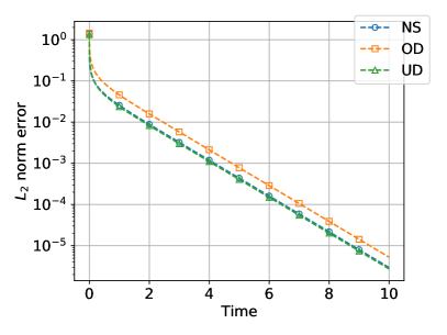
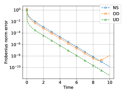
Figure 23: $L_{2}$ error $\lVert m_{n}-m_{ref}\rVert_{2}$ (left) and Frobenius norm $\lVert C_{n}-C_{ref}\rVert_{F}$ (right) obtained by UKS for non-singular (NS), over-determined (OD), and under-determined (UD) systems of the linear 2-parameter model problem.

B.2 Nonlinear 2-Parameter Model Problem

The following Bayesian logistic regression problem is considered,

$$y=\frac{1}{1+\exp(\theta_{(1)}+\theta_{(2)}x)}+\eta.$$

Here $N_{\theta}=2$ and $N_{y}=1$, and hence this is an under-determined problem. The prior distribution $\mathcal{N}(r_{0},\Sigma_{0})$ satisfies

$$r_{0}=[1\quad 1]^{T}\quad\textrm{ and }\quad\Sigma_{0}=\mathbb{I}.$$

The observation data $y_{ref}=0.08$ is generated at $x=\frac{1}{2}$, with observation error $\eta\sim\mathcal{N}(0,0.1^{2})$ and $\theta_{ref}=[2\quad 2]^{T}$.

The UKS is initialized with $\theta_{0}\sim\mathcal{N}(r_{0},\Sigma_{0})$. The posterior distributions obtained by the UKS at $t=10$ with a time step $h=5\times 10^{-5}$ and Markov chain Monte Carlo method (MCMC) with a step size $1.0$ and $5\times 10^{6}$ samples (with a $10^{6}$ sample burn-in period) are presented in Fig. 24. The estimated posterior distributions are in reasonably good agreement, but of course not as accurate as in the linear setting in the previous subsection, because of a Gaussian approximation being made to a non-Gaussian distribution. Specifically, the posterior mean and covariance estimated by the UKS are

$$[1.41\quad 1.20]^{T}\quad\textrm{ and }\quad\begin{bmatrix}0.526&-0.235\\ -0.235&0.884\\ \end{bmatrix},$$

whilst the posterior mean and covariance estimated by the MCMC are

$$[1.62\quad 1.31]^{T}\quad\textrm{ and }\quad\begin{bmatrix}0.619&-0.254\\ -0.254&1.00\\ \end{bmatrix}.$$

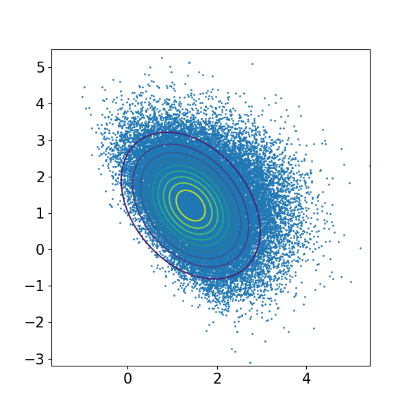
Figure 24: Contour plot: posterior distributions obtained by UKS at $t=10$; blue dots: reference posterior distribution obtained by MCMC for the nonlinear 2-parameter model problem. x-axis is for $\theta_{(1)}$ and y-axis is for $\theta_{(2)}$.

References

- [1] Marco A Iglesias, Kody JH Law, and Andrew M Stuart. Ensemble Kalman methods for inverse problems. Inverse Problems, 29(4):045001, 2013.
- [2] Marco A Iglesias. A regularizing iterative ensemble Kalman method for pde-constrained inverse problems. Inverse Problems, 32(2):025002, 2016.
- [3] Marco Iglesias and Yuchen Yang. Adaptive regularisation for ensemble Kalman inversion. Inverse Problems, 37(2):025008, 2021.
- [4] Neil K Chada, Andrew M Stuart, and Xin T Tong. Tikhonov regularization within ensemble Kalman inversion. SIAM Journal on Numerical Analysis, 58(2):1263–1294, 2020.
- [5] Claudia Schillings and Andrew M Stuart. Analysis of the ensemble Kalman filter for inverse problems. SIAM Journal on Numerical Analysis, 55(3):1264–1290, 2017.
- [6] Alfredo Garbuno-Inigo, Franca Hoffmann, Wuchen Li, and Andrew M Stuart. Interacting langevin diffusions: gradient structure and ensemble Kalman sampler. SIAM Journal on Applied Dynamical Systems, 19(1):412–441, 2020.
- [7] Alfredo Garbuno-Inigo, Nikolas Nüsken, and Sebastian Reich. Affine invariant interacting langevin dynamics for bayesian inference. SIAM Journal on Applied Dynamical Systems, 19(3):1633–1658, 2020.
- [8] Zhiyan Ding, Qin Li, and Jianfeng Lu. Ensemble Kalman inversion for nonlinear problems: weights, consistency, and variance bounds. arXiv preprint arXiv:2003.02316, 2020.
- [9] Daniel Zhengyu Huang, Jiaoyang Huang, Sebastian Reich, and Andrew M Stuart. Efficient derivative-free bayesian inference for large-scale inverse problems. arXiv preprint arXiv:2204.04386, 2022.
- [10] Sebastian Reich and Simon Weissmann. Fokker–planck particle systems for bayesian inference: Computational approaches. SIAM/ASA Journal on Uncertainty Quantification, 9(2):446–482, 2021.
- [11] Zhiyan Ding and Qin Li. Ensemble Kalman inversion: mean-field limit and convergence analysis. Statistics and Computing, 31(1):1–21, 2021.
- [12] Zhiyan Ding and Qin Li. Ensemble Kalman sampler: Mean-field limit and convergence analysis. SIAM Journal on Mathematical Analysis, 53(2):1546–1578, 2021.
- [13] Heinz Werner Engl, Martin Hanke, and Andreas Neubauer. Regularization of inverse problems, volume 375. Springer Science & Business Media, 1996.
- [14] Jari Kaipio and Erkki Somersalo. Statistical and computational inverse problems, volume 160. Springer Science & Business Media, 2006.
- [15] Masoumeh Dashti and Andrew M Stuart. The bayesian approach to inverse problems. arXiv preprint arXiv:1302.6989, 2013.
- [16] Pierre Del Moral, Arnaud Doucet, and Ajay Jasra. Sequential monte carlo samplers. Journal of the Royal Statistical Society: Series B (Statistical Methodology), 68(3):411–436, 2006.
- [17] Nicolas Chopin, Omiros Papaspiliopoulos, et al. An introduction to sequential Monte Carlo, volume 4. Springer, 2020.
- [18] Alexandros Beskos, Ajay Jasra, Ege A Muzaffer, and Andrew M Stuart. Sequential monte carlo methods for bayesian elliptic inverse problems. Statistics and Computing, 25(4):727–737, 2015.
- [19] Sebastian Reich. A dynamical systems framework for intermittent data assimilation. BIT Numerical Mathematics, 51(1):235–249, 2011.
- [20] Peter Lancaster and Leiba Rodman. Algebraic riccati equations. Clarendon press, 1995.
- [21] Philippe Bougerol. Kalman filtering with random coefficients and contractions. SIAM Journal on Control and Optimization, 31(4):942–959, 1993.
- [22] Rudolph Emil Kalman. A new approach to linear filtering and prediction problems. J. Basic Eng. Mar, 82(1):35–45, 1960.
- [23] Harold Wayne Sorenson. Kalman filtering: theory and application. IEEE, 1985.
- [24] Andrew H Jazwinski. Stochastic processes and filtering theory. Courier Corporation, 2007.
- [25] Michael Ghil, S Cohn, John Tavantzis, K Bube, and Eugene Isaacson. Applications of estimation theory to numerical weather prediction. In Dynamic meteorology: Data assimilation methods, pages 139–224. Springer, 1981.
- [26] Geir Evensen. Sequential data assimilation with a nonlinear quasi-geostrophic model using monte carlo methods to forecast error statistics. Journal of Geophysical Research: Oceans, 99(C5):10143–10162, 1994.
- [27] Yan Chen and Dean S Oliver. Ensemble randomized maximum likelihood method as an iterative ensemble smoother. Mathematical Geosciences, 44(1):1–26, 2012.
- [28] Alexandre A Emerick and Albert C Reynolds. Investigation of the sampling performance of ensemble-based methods with a simple reservoir model. Computational Geosciences, 17(2):325–350, 2013.
- [29] Martin Hanke. A regularizing levenberg-marquardt scheme, with applications to inverse groundwater filtration problems. Inverse problems, 13(1):79, 1997.
- [30] Nikolas Nüsken and Sebastian Reich. Note on interacting langevin diffusions: Gradient structure and ensemble Kalman sampler by garbuno-inigo, hoffmann, li and stuart. arXiv preprint arXiv:1908.10890, 2019.
- [31] Kody JH Law and Andrew M Stuart. Evaluating data assimilation algorithms. Monthly Weather Review, 140(11):3757–3782, 2012.
- [32] Oliver G Ernst, Björn Sprungk, and Hans-Jörg Starkloff. Analysis of the ensemble and polynomial chaos Kalman filters in bayesian inverse problems. SIAM/ASA Journal on Uncertainty Quantification, 3(1):823–851, 2015.
- [33] GA Pavliotis, AM Stuart, and U. Vaes. Derivative-free bayesian inversion using multiscale dynamics. arXiv preprint arXiv:2102.00540, 2021.
- [34] Simon J Julier, Jeffrey K Uhlmann, and Hugh F Durrant-Whyte. A new approach for filtering nonlinear systems. In Proceedings of 1995 American Control Conference-ACC’95, volume 3, pages 1628–1632. IEEE, 1995.
- [35] Eric A Wan and Rudolph Van Der Merwe. The unscented Kalman filter for nonlinear estimation. In Proceedings of the IEEE 2000 Adaptive Systems for Signal Processing, Communications, and Control Symposium (Cat. No. 00EX373), pages 153–158. Ieee, 2000.
- [36] Mrinal K Sen and Paul L Stoffa. Global optimization methods in geophysical inversion. Cambridge University Press, 2013.
- [37] Tapio Schneider, Shiwei Lan, Andrew Stuart, and Joao Teixeira. Earth system modeling 2.0: A blueprint for models that learn from observations and targeted high-resolution simulations. Geophysical Research Letters, 44(24):12–396, 2017.
- [38] Oliver RA Dunbar, Alfredo Garbuno-Inigo, Tapio Schneider, and Andrew M Stuart. Calibration and uncertainty quantification of convective parameters in an idealized gcm. arXiv preprint arXiv:2012.13262, 2020.
- [39] Daniel Z Huang, Kailai Xu, Charbel Farhat, and Eric Darve. Learning constitutive relations from indirect observations using deep neural networks. Journal of Computational Physics, page 109491, 2020.
- [40] Kailai Xu, Daniel Z Huang, and Eric Darve. Learning constitutive relations using symmetric positive definite neural networks. Journal of Computational Physics, 428:110072, 2020.
- [41] Philip Avery, Daniel Z Huang, Wanli He, Johanna Ehlers, Armen Derkevorkian, and Charbel Farhat. A computationally tractable framework for nonlinear dynamic multiscale modeling of membrane fabric. arXiv preprint arXiv:2007.05877, 2020.
- [42] Brian H Russell. Introduction to seismic inversion methods. SEG Books, 1988.
- [43] Carey Bunks, Fatimetou M Saleck, S Zaleski, and G Chavent. Multiscale seismic waveform inversion. Geophysics, 60(5):1457–1473, 1995.
- [44] Johannes Töger, Matthew J Zahr, Nicolas Aristokleous, Karin Markenroth Bloch, Marcus Carlsson, and Per-Olof Persson. Blood flow imaging by optimal matching of computational fluid dynamics to 4d-flow data. Magnetic Resonance in Medicine, 2020.
- [45] Flávio Celso Trigo, Raul Gonzalez-Lima, and Marcelo Britto Passos Amato. Electrical impedance tomography using the extended Kalman filter. IEEE Transactions on Biomedical Engineering, 51(1):72–81, 2004.
- [46] Dan Simon. Optimal state estimation: Kalman, H infinity, and nonlinear approaches. John Wiley & Sons, 2006.
- [47] François Auger, Mickael Hilairet, Josep M Guerrero, Eric Monmasson, Teresa Orlowska-Kowalska, and Seiichiro Katsura. Industrial applications of the Kalman filter: A review. IEEE Transactions on Industrial Electronics, 60(12):5458–5471, 2013.
- [48] Huazhen Fang, Ning Tian, Yebin Wang, MengChu Zhou, and Mulugeta A Haile. Nonlinear bayesian estimation: from Kalman filtering to a broader horizon. IEEE/CAA Journal of Automatica Sinica, 5(2):401–417, 2018.
- [49] Sharad Singhal and Lance Wu. Training multilayer perceptrons with the extended Kalman algorithm. In Advances in neural information processing systems, pages 133–140, 1989.
- [50] Gintaras V Puskorius and Lee A Feldkamp. Decoupled extended Kalman filter training of feedforward layered networks. In IJCNN-91-Seattle International Joint Conference on Neural Networks, volume 1, pages 771–777. IEEE, 1991.
- [51] Zhengyu Huang, Philip Avery, Charbel Farhat, Jason Rabinovitch, Armen Derkevorkian, and Lee D Peterson. Simulation of parachute inflation dynamics using an eulerian computational framework for fluid-structure interfaces evolving in high-speed turbulent flows. In 2018 AIAA Aerospace Sciences Meeting, page 1540, 2018.
- [52] Daniel Z Huang, P-O Persson, and Matthew J Zahr. High-order, linearly stable, partitioned solvers for general multiphysics problems based on implicit–explicit runge–kutta schemes. Computer Methods in Applied Mechanics and Engineering, 346:674–706, 2019.
- [53] Daniel Z Huang, Philip Avery, Charbel Farhat, Jason Rabinovitch, Armen Derkevorkian, and Lee D Peterson. Modeling, simulation and validation of supersonic parachute inflation dynamics during mars landing. In AIAA Scitech 2020 Forum, page 0313, 2020.
- [54] Daniel Z Huang, Will Pazner, Per-Olof Persson, and Matthew J Zahr. High-order partitioned spectral deferred correction solvers for multiphysics problems. Journal of Computational Physics, page 109441, 2020.
- [55] Alistair Adcroft, Whit Anderson, V Balaji, Chris Blanton, Mitchell Bushuk, Carolina O Dufour, John P Dunne, Stephen M Griffies, Robert Hallberg, Matthew J Harrison, et al. The gfdl global ocean and sea ice model om4. 0: Model description and simulation features. Journal of Advances in Modeling Earth Systems, 11(10):3167–3211, 2019.
- [56] Charles S Peskin. Numerical analysis of blood flow in the heart. Journal of computational physics, 25(3):220–252, 1977.
- [57] Marsha Berger and Michael Aftosmis. Progress towards a cartesian cut-cell method for viscous compressible flow. In 50th AIAA Aerospace Sciences Meeting Including the New Horizons Forum and Aerospace Exposition, page 1301, 2012.
- [58] Daniel Z Huang, Dante De Santis, and Charbel Farhat. A family of position-and orientation-independent embedded boundary methods for viscous flow and fluid–structure interaction problems. Journal of Computational Physics, 365:74–104, 2018.
- [59] Daniel Z Huang, Philip Avery, and Charbel Farhat. An embedded boundary approach for resolving the contribution of cable subsystems to fully coupled fluid-structure interaction. International Journal for Numerical Methods in Engineering, 2020.
- [60] Marsha J Berger, Phillip Colella, et al. Local adaptive mesh refinement for shock hydrodynamics. Journal of computational Physics, 82(1):64–84, 1989.
- [61] Raunak Borker, Daniel Huang, Sebastian Grimberg, Charbel Farhat, Philip Avery, and Jason Rabinovitch. Mesh adaptation framework for embedded boundary methods for computational fluid dynamics and fluid-structure interaction. International Journal for Numerical Methods in Fluids, 90(8):389–424, 2019.
- [62] Emmet Cleary, Alfredo Garbuno-Inigo, Shiwei Lan, Tapio Schneider, and Andrew M Stuart. Calibrate, emulate, sample. Journal of Computational Physics, 424:109716, 2020.
- [63] Daniel J Lea, Myles R Allen, and Thomas WN Haine. Sensitivity analysis of the climate of a chaotic system. Tellus A: Dynamic Meteorology and Oceanography, 52(5):523–532, 2000.
- [64] Qiqi Wang, Rui Hu, and Patrick Blonigan. Least squares shadowing sensitivity analysis of chaotic limit cycle oscillations. Journal of Computational Physics, 267:210–224, 2014.
- [65] Nikola B Kovachki and Andrew M Stuart. Ensemble Kalman inversion: a derivative-free technique for machine learning tasks. Inverse Problems, 35(9):095005, 2019.
- [66] Dean S Oliver, Albert C Reynolds, and Ning Liu. Inverse theory for petroleum reservoir characterization and history matching. Cambridge University Press, 2008.
- [67] Eric A Wan and Alex T Nelson. Neural dual extended Kalman filtering: applications in speech enhancement and monaural blind signal separation. In Neural Networks for Signal Processing VII. Proceedings of the 1997 IEEE Signal Processing Society Workshop, pages 466–475. IEEE, 1997.
- [68] Alexander G Parlos, Sunil K Menon, and A Atiya. An algorithmic approach to adaptive state filtering using recurrent neural networks. IEEE Transactions on Neural Networks, 12(6):1411–1432, 2001.
- [69] JH Gove and DY Hollinger. Application of a dual unscented Kalman filter for simultaneous state and parameter estimation in problems of surface-atmosphere exchange. Journal of Geophysical Research: Atmospheres, 111(D8), 2006.
- [70] David J Albers, Matthew Levine, Bruce Gluckman, Henry Ginsberg, George Hripcsak, and Lena Mamykina. Personalized glucose forecasting for type 2 diabetes using data assimilation. PLoS computational biology, 13(4):e1005232, 2017.
- [71] Kay Bergemann and Sebastian Reich. An ensemble Kalman-Bucy filter for continuous data assimilation. Meteorologische Zeitschrift, 21(3):213–219, 2012.
- [72] Claudia Schillings and Andrew M Stuart. Convergence analysis of ensemble Kalman inversion: the linear, noisy case. Applicable Analysis, 97(1):107–123, 2018.
- [73] Zhiyan Ding and Qin Li. Ensemble Kalman inversion: mean-field limit and convergence analysis. arXiv preprint arXiv:1908.05575, 2019.
- [74] Bradley M Bell and Frederick W Cathey. The iterated Kalman filter update as a gauss-newton method. IEEE Transactions on Automatic Control, 38(2):294–297, 1993.
- [75] Neil K Chada and Xin T Tong. Convergence acceleration of ensemble Kalman inversion in nonlinear settings. arXiv preprint arXiv:1911.02424, 2019.
- [76] Neil K Chada, Yuming Chen, and Daniel Sanz-Alonso. Iterative ensemble Kalman methods: A unified perspective with some new variants. arXiv preprint arXiv:2010.13299, 2020.
- [77] José A Carrillo, Young-Pil Choi, Claudia Totzeck, and Oliver Tse. An analytical framework for consensus-based global optimization method. Mathematical Models and Methods in Applied Sciences, 28(06):1037–1066, 2018.
- [78] José A Carrillo, Franca Hoffmann, Andrew M Stuart, and Urbain Vaes. Consensus based sampling. arXiv, 2021.
- [79] Sebastian Reich and Colin Cotter. Probabilistic forecasting and Bayesian data assimilation. Cambridge University Press, 2015.
- [80] Kody Law, Andrew Stuart, and Kostas Zygalakis. Data assimilation. Cham, Switzerland: Springer, 2015.
- [81] Daniel Sanz-Alonso, Andrew M Stuart, and Armeen Taeb. Inverse problems and data assimilation. arXiv preprint arXiv:1810.06191, 2018.
- [82] Jonathan Goodman and Jonathan Weare. Ensemble samplers with affine invariance. Communications in applied mathematics and computational science, 5(1):65–80, 2010.
- [83] John A Nelder and Roger Mead. A simplex method for function minimization. The computer journal, 7(4):308–313, 1965.
- [84] Benedict Leimkuhler, Charles Matthews, and Jonathan Weare. Ensemble preconditioning for markov chain monte carlo simulation. Statistics and Computing, 28(2):277–290, 2018.
- [85] Simon Julier, Jeffrey Uhlmann, and Hugh F Durrant-Whyte. A new method for the nonlinear transformation of means and covariances in filters and estimators. IEEE Transactions on automatic control, 45(3):477–482, 2000.
- [86] Michael K Tippett, Jeffrey L Anderson, Craig H Bishop, Thomas M Hamill, and Jeffrey S Whitaker. Ensemble square root filters. Monthly Weather Review, 131(7):1485–1490, 2003.
- [87] Lehel Csató and Manfred Opper. Sparse on-line gaussian processes. Neural computation, 14(3):641–668, 2002.
- [88] David J Albers, Paul-Adrien Blancquart, Matthew E Levine, Elnaz Esmaeilzadeh Seylabi, and Andrew Stuart. Ensemble Kalman methods with constraints. Inverse Problems, 35(9):095007, 2019.
- [89] JA Carrillo and U Vaes. Wasserstein stability estimates for covariance-preconditioned fokker–planck equations. arXiv preprint arXiv:1910.07555, 2019.
- [90] Lassi Roininen, Janne MJ Huttunen, and Sari Lasanen. Whittle-matérn priors for bayesian statistical inversion with applications in electrical impedance tomography. Inverse Problems & Imaging, 8(2):561, 2014.
- [91] Marco A Iglesias, Kody JH Law, and Andrew M Stuart. Evaluation of gaussian approximations for data assimilation in reservoir models. Computational Geosciences, 17(5):851–885, 2013.
- [92] Bernhard Beckermann. The condition number of real vandermonde, krylov and positive definite hankel matrices. Numerische Mathematik, 85(4):553–577, 2000.
- [93] Matthew M Dunlop, Marco A Iglesias, and Andrew M Stuart. Hierarchical bayesian level set inversion. Statistics and Computing, 27(6):1555–1584, 2017.
- [94] Nicholas H Nelsen and Andrew M Stuart. The random feature model for input-output maps between banach spaces. arXiv preprint arXiv:2005.10224, 2020.
- [95] Jan S Hesthaven, Sigal Gottlieb, and David Gottlieb. Spectral methods for time-dependent problems, volume 21. Cambridge University Press, 2007.
- [96] Steven A Orszag and GS Patterson Jr. Numerical simulation of three-dimensional homogeneous isotropic turbulence. Physical Review Letters, 28(2):76, 1972.
- [97] Edward N Lorenz. Deterministic nonperiodic flow. In The Theory of Chaotic Attractors, pages 25–36. Springer, 2004.
- [98] Wael Bahsoun, Ian Melbourne, and Marks Ruziboev. Variance continuity for lorenz flows. In Annales Henri Poincare, volume 21, pages 1873–1892. Springer, 2020.
- [99] Jan Frøyland and Knut H Alfsen. Lyapunov-exponent spectra for the lorenz model. Physical Review A, 29(5):2928, 1984.
- [100] Edward N Lorenz. Predictability: A problem partly solved. In Proc. Seminar on predictability, volume 1, 1996.
- [101] Ibrahim Fatkullin and Eric Vanden-Eijnden. A computational strategy for multiscale systems with applications to lorenz 96 model. Journal of Computational Physics, 200(2):605–638, 2004.
- [102] Daniel S Wilks. Effects of stochastic parametrizations in the lorenz’96 system. Quarterly Journal of the Royal Meteorological Society: A journal of the atmospheric sciences, applied meteorology and physical oceanography, 131(606):389–407, 2005.
- [103] HM Arnold, IM Moroz, and TN Palmer. Stochastic parametrizations and model uncertainty in the lorenz’96 system. Philosophical Transactions of the Royal Society A: Mathematical, Physical and Engineering Sciences, 371(1991):20110479, 2013.
- [104] Georg A Gottwald and Sebastian Reich. Supervised learning from noisy observations: Combining machine-learning techniques with data assimilation. arXiv preprint arXiv:2007.07383, 2020.
- [105] Isaac M Held and Max J Suarez. A proposal for the intercomparison of the dynamical cores of atmospheric general circulation models. Bulletin of the American Meteorological society, 75(10):1825–1830, 1994.