Physical properties of Brightest Cluster Galaxies up to redshift 1.80 based on HST data

Abstract

Context. Brightest cluster galaxies (BCGs) have grown by accreting numerous smaller galaxies and can be used as tracers of cluster formation and evolution in the cosmic web. However, there is still a controversy on the main epoch of formation of BCGs, since some authors believe they have already formed before redshift z=2, while others still find them to evolve at more recent epochs.

Aims. We aim to analyse the physical properties of a large sample of BCGs covering a wide redshift range up to z=1.8 and analysed in a homogeneous way, to see if their characteristics vary with redshift. As a first step, we also present a new tool to define for each cluster which galaxy is the BCG.

Methods. For a sample of 137 clusters with HST images in the optical and/or infrared, we analyse the BCG properties by applying GALFIT with one or two Sérsic components. For each BCG, we thus compute the Sérsic index, effective radius, major axis position angle, surface brightness. We then search for correlations of these quantities with redshift.

Results. We find that the BCGs follow the Kormendy relation (between the effective radius and the mean surface brightness), with a slope that remains constant with redshift, but with a variation with redshift of the ordinate at the origin. Although the trends are faint, we find that both the absolute magnitudes and effective radii tend to become respectively brighter and bigger with decreasing redshift. On the other hand, we find no significant correlation of the mean surface brightnesses or Sérsic indices with redshift. The major axes of the cluster elongations and of the BCGs agree within 30 degrees for 73% of our clusters at redshift z $\leq$ 0.9.

Conclusions. Our results agree with the BCGs being mainly formed before redshift z=2. The alignment of the major axes of BCGs with their clusters agree with the general idea that BCGs form at the same time as clusters by accreting matter along the filaments of the cosmic web.

1 Introduction

Galaxy clusters are the largest and most massive gravitationally bound structures observed in the Universe. As so, they constitute perfect probes to test cosmological models and help us better understand the history of the Universe, as they will constrain the limits of observed physical parameters through time, such as mass or brightness, in numerical simulations (Kravtsov & Borgani, 2012). The $\Lambda$CDM model proposes a hierarchical evolution scenario starting from small fluctuations that assemble together via the gravitational force, and grow to form bigger and bigger structures. As a result, galaxy clusters are the latest and most massive structures to have formed.

Clusters are believed to be located at the intersection of cosmic filaments, and to form by merging with other smaller clusters or groups of galaxies, and by constantly accreting gas and galaxies that preferentially move along cosmic filaments and end up falling towards the center of the gravitational potential well, which often coincides with the peak of the X-ray emission (see De Propris et al., 2020, and references therein). Generally, the brightest galaxy of the cluster, the Brightest Cluster Galaxy (BCG hereafter) lies at the center of the cluster. It is usually a supermassive elliptical galaxy, that is formed and grows by mergers with other galaxies, and can be up to two magnitudes brighter than the second brightest galaxy. This property makes BCGs easily recognisable. BCGs have often been referred to as cD galaxies, i.e. supergiant ellipticals with a large and diffuse halo of stars. Since their properties are closely linked to those of their host cluster (Lauer et al., 2014), they can be extremely useful to trace how galaxy clusters have formed and evolved. BCGs tend to be aligned along the major axis of the cluster, which also hints at the close link between the BCG and its host cluster (Donahue et al., 2015; Durret et al., 2016; West et al., 2017; De Propris et al., 2020). This alignment suggests that the accretion of galaxies may be done along a preferential axis, with galaxies falling into clusters along cosmic filaments.

Most of the stars in today’s BCGs were already formed at redshift $z\geq 2$ (Thomas et al., 2010). BCGs, especially the most massive ones, can present an extended halo made of stars that were stripped from their host galaxy during mergers, and form the Intra Cluster Light (ICL). When measuring photometric properties of galaxies, some parameters such as the BCG major axis can be difficult to measure accurately as the separation between the ICL and the external envelope of the BCG is not clear. However, the ICL is a very faint component, and as we are observing bright galaxies, the ICL should not strongly affect our study, so the ICL will not be considered in this paper.

The evolution of BCG properties with redshift is of interest to study cluster formation and evolution, but this topic remains quite controversial. Some authors report no evolution of the sizes of the BCGs with redshift (see Bai et al., 2014; Stott et al., 2011, and references therein): Stott et al. (2011) found that there was no significant evolution of the sizes or shapes of the BCGs between redshift 0.25 and 1.3; whereas Ascaso et al. (2010) found that, although the shapes show little change, they have grown by a factor of 2 in the last 6 Gyrs. Bernardi (2009) found a 70% increase of the sizes of BCGs since z = 0.25, and an increase of a factor 2 since z = 0.5.

Bai et al. (2014) found that while the inner region of the galaxies doesn’t grow much, the light dispersed around the BCG forms the outer component, resulting in a shallow outer luminosity profile. This is an indication of an inside-out growth of BCGs: the inner component forms first and then stops growing while the outer component develops. Edwards et al. (2019) gave more evidence to justify this inside-out growth of BCGs by showing that the stars in the ICL are younger and less metal-rich than those in the cores of the BCGs. They also showed that the most extended BCGs tend to be close to the X-ray center. This last statement is supported by Lauer et al. (2014), who added that the inner component would have already been formed before the cluster, while the outer component, the envelope of the BCG, is formed and grows later. In fact, numerical simulations with AGN suppressed cooling flows, showed that about 80% of the stars are already formed at redshift z $\approx$ 3 in the BCG progenitors that merge together to form today’s BCGs (De Lucia & Blaizot, 2007). Cooke et al. (2019b) found that BCG progenitors in the COSMOS field have an active star formation phase before z = 2.25, followed by a phase of dry and wet mergers until z = 1.25 that leads to more star formation and increases the stellar mass of the progenitors, after which the stellar mass of progenitors mainly grows through dry mergers, and half of the stellar mass is formed at z = 0.5. Similarly, Cerulo et al. (2019) did not find significant stellar mass growth between z = 0.35 and z = 0.05, suggesting that most of the BCGs stellar masses were formed by z = 0.35. Durret et al. (2019) observed a possible variation with redshift of the effective radius of the outer Sérsic component of BCGs for 38 BCGs in the redshift range 0.2 $\leq$ z $\leq$ 0.9, agreeing with a scenario in which BCGs at these redshifts mostly grow by accreting smaller galaxies.

Several conflicts also arise on the growth of the stellar masses of the BCGs: Collins & Mann (1998); Collins et al. (2009); Stott et al. (2010) found little to no evolution. On the other hand, other studies found a strong evolution in the stellar masses of BCGs since redshift z = 2 (Aragon-Salamanca et al., 1998; Lidman et al., 2012; Lin et al., 2013; Bellstedt et al., 2016; Zhang et al., 2016).

In the present paper, we will try to characterize how the properties of BCGs have evolved since z = 1.80, based on HST data to have the best possible spatial resolution, which is particularly necessary at high redshift. When dealing with a large amount of data, identifying individually the BCG of a cluster to build a sample can be a long task to do. This is why we present here a method based on several photometric properties of the BCGs, that will allow to detect BCGs automatically. We analyze a sample of 137 galaxy clusters, covering the redshift range 0.187 $\leq$ z $\leq$ 1.80, and including various types of BCGs (star forming BCGs, SF BCGs hereafter, interacting BCGs, hosts of possible AGNs, supercluster members, etc.).

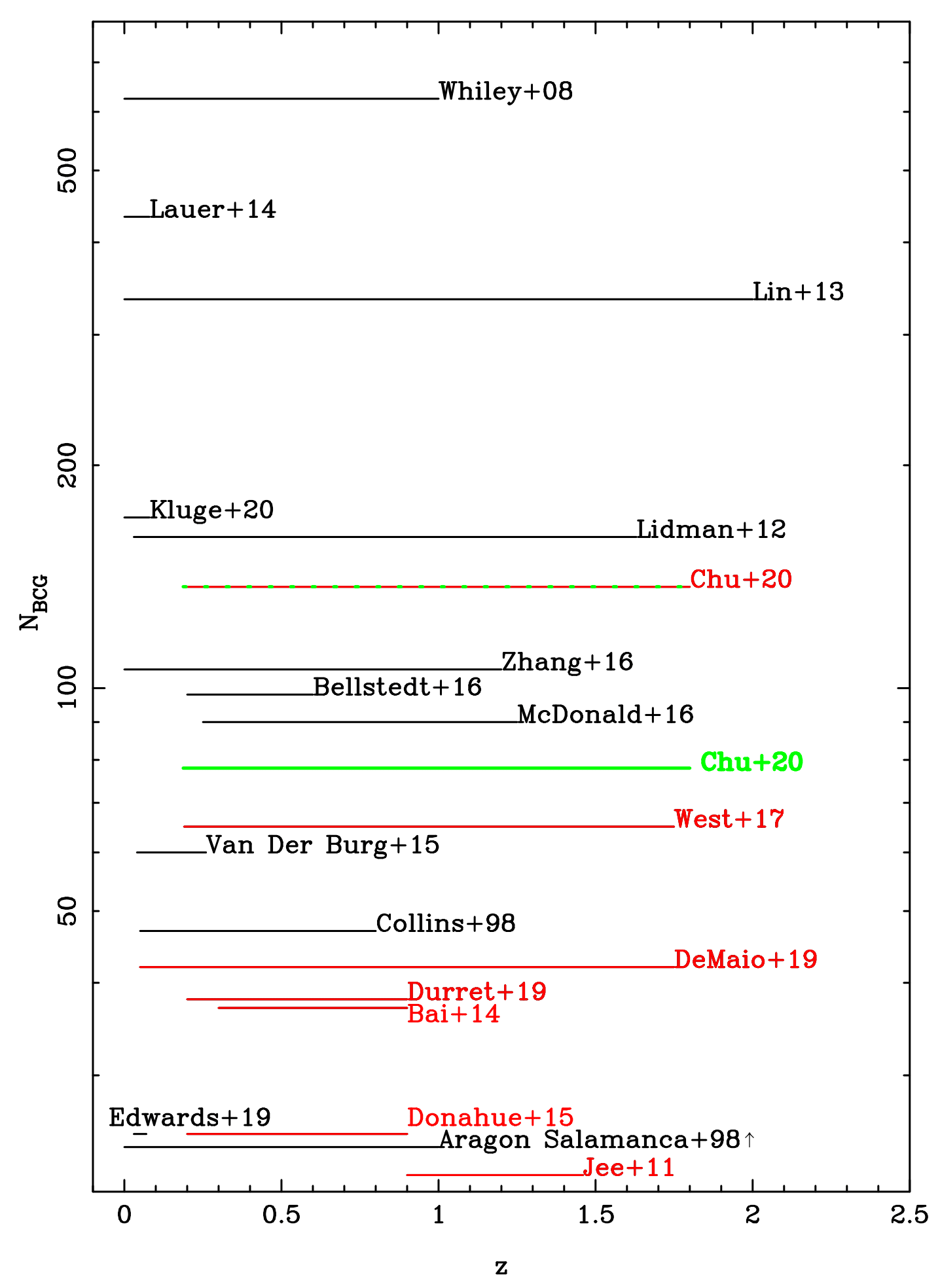
Figure 1: Comparison of the various samples of BCGs found in the literature, considering the redshift range, the number of galaxies analysed and the type of data used. Only samples with at least 20 objects are represented here. Cerulo et al. (2019) with a sample of 74275 BCGs is not represented here for better lisibility. The samples represented in black use ground-based telescope data, space-based data excluding HST, or a mix of ground-based and space-based data, while those in red only use HST data. Our initial sample is represented by the red and green dotted line, and our final BCG sample in green (see Section 4).

The present paper (in green in Figure 1, the figure will be described in more detail in the next section) will allow to cover a large redshift range with one of the largest samples observed with HST (indicated in red). This will enable us to obtain more significant statistics on the evolution of BCG properties.

The paper is organized as follows. We will describe the data in Section 2, the method to detect automatically the BCGs in Section 3, and the modelization of their luminosity profiles in Section 4. The results obtained as well as a short study of the link between the BCG masses, distance between the BCG and the X-ray center of the cluster, and physical properties are given in Section 5. A final discussion and conclusions are presented in Section 6.

Throughout this paper, we assume H₀ = 70 km s^-1 Mpc^-1, $\Omega_{M}$ = 0.3 and $\Omega_{\Lambda}$ = 0.7. The scales and physical distances are computed using the astropy.coordinates package. Unless specified, all magnitudes are given in the AB system.

2 Sample and data

2.1 The sample

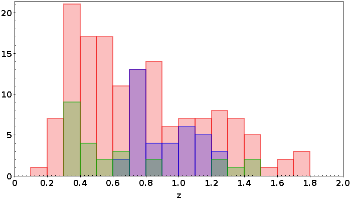
Figure 2: Histogram of the redshifts of the 149 BCGs in our sample. The red histogram shows all the BCGs studied while the blue histogram (37 BCGs) shows those observed in too blue rest frame filters compared to the 4000 Å break (see Section 3). The green histogram (25 BCGs) shows all BCGs with an important inner component (see Section 4).

The sample studied in this paper consists of 137 galaxy clusters with HST imaging taken from Jee et al. (2011); Postman et al. (2012b); Bai et al. (2014); Donahue et al. (2015); West et al. (2017); DeMaio et al. (2019); Durret et al. (2019); Sazonova et al. (2020) . We also add five more distant clusters at z $\geq$ 0.8, as well as the cluster Abell 2813 at z = 0.29. Among them, we identify twelve clusters which present in their center two BCGs similar in magnitude and size (see Section 3). As a result, our final BCG sample contains 149 BCGs (the number of BCGs is not equal to the number of clusters studied because of these clusters with two BCGs). This sample is a good representation of the most massive BCGs in the range 0.1 $\leq$ z $\leq$ 1.80. The redshift distribution is shown on Figure 2.

All of these clusters have data available from the Hubble Space Telescope, obtained with the Advanced Camera for Surveys (ACS) in optical bands and/or the Wide Field Camera 3 (WFC3) in infrared bands, resulting in good quality images. This allows us to perform accurate photometry with relatively good precision, and to treat all the BCGs in a homogeneous way. Contrary to other studies such as Bai et al. (2014), we do not exclude in our study clusters with bright nearby objects that may hinder our measurements near the BCG area. We also identify in our sample two clusters host of blue BCGs (negative rest frame blue-red color), with active star forming regions inside the BCGs. These two BCGs will be described more in details in Section 3.

Our sample covers a large range in redshift, which will enable us to trace the history of cluster formation through time.

Figure 1 shows the comparison of the sample sizes and redshift ranges between different studies done on BCGs. Cerulo et al. (2019) studied a sample 74275 BCGs from the SDSS in the redshift range 0.05 $\leq$ z $\leq$ 0.35, and is not represented on this figure for better lisibility. Most large studies, especially those with HST data (represented in red), were done exclusively on local BCGs (z $\leq$ 0.1) (Lauer et al., 2014; Cerulo et al., 2019), while farther clusters and BCGs were limited to relatively small samples (N $\leq$ 45) (Bai et al., 2014; DeMaio et al., 2019; Durret et al., 2019) and/or used ground-based data (represented in black). Our sample contains more clusters and BCGs at high redshifts (z $\geq$ 0.7) than that of Lidman et al. (2012) (33 in Lidman et al., 2012, 73 in this paper). With the present study, we therefore almost double the previous samples and cover a larger range in redshift. This enables us to obtain more significant statistics on the evolution of BCG properties.

Lidman et al. (2012), Lin et al. (2013), West et al. (2017) and De Propris et al. (2020) mainly focus on the alignment of the BCGs with their host cluster and on the evolution of the BCG stellar masses. Our work constitutes a deeper analysis since we also study the luminosity profiles of the BCGs.

2.2 Retrieving data and cluster information

We retrieve all the FITS images from the Hubble Legacy Archive (HLA). We look for combined or mosaic images according to what is available and download stacked images directly from the HLA. To avoid handling such heavy files, we first crop these images, define the new center on the cluster coordinates found in NED, and create a new image 1.2 Mpc wide. Linear scales (arcsec/Mpc) are determined from the cluster redshifts in the literature (from Jee et al., 2011; Postman et al., 2012b; Bai et al., 2014; Donahue et al., 2015; West et al., 2017; DeMaio et al., 2019; Durret et al., 2019; Sazonova et al., 2020, or found in NED for the five other clusters we added). Cluster information can be found in Table 1. It is necessary to add the keywords ’GAIN’ and ’RDNOISE’ in the header of the FITS images, which will be used later by SExtractor or GALFIT. As the images are in units of electrons/s, we set the GAIN to 1 and multiply the images by the total exposure time (EXPTIME) to get back to units in electrons. Single exposure images were summed with AstroDrizzle to get the final combined images. We also retrieve the associated weight maps (wht fits) obtained applying the option IVM (Inverse Variance Map) of AstroDrizzle.

3 Procedure for the detection of the BCG

The definition of the BCG that we use throughout this paper is the following: the BCG is the brightest galaxy of the cluster that lies close to the cluster center, defined as the center of the cluster member galaxy distribution. Generally, the cluster center is defined as the X-ray center of the cluster, as X-rays trace the mass distribution better. However, it is difficult to obtain X-ray data, particularly at high redshifts. If a large sample is considered, most probably a good fraction of the clusters do not have X-ray data available. Moreover, it was shown in several studies (Patel et al., 2006; Hashimoto et al., 2014; De Propris et al., 2020) that BCGs are often displaced from the X-ray center. For these reasons and anticipating for future works with much larger samples, we use a definition which is independent from X-rays and only relies on optical and infrared photometric data. We define the center as that of the spatial distribution of cluster galaxies (as in Kluge et al., 2020). As a matter of fact, X-ray coordinates are only available for 68 out of the 137 clusters in our sample (see Table 4). These X-ray positions will only be used to study whether or not the BCG properties correlate with their position relatively to the X-ray center (see Section 5).

3.1 Method for detecting red BCGs

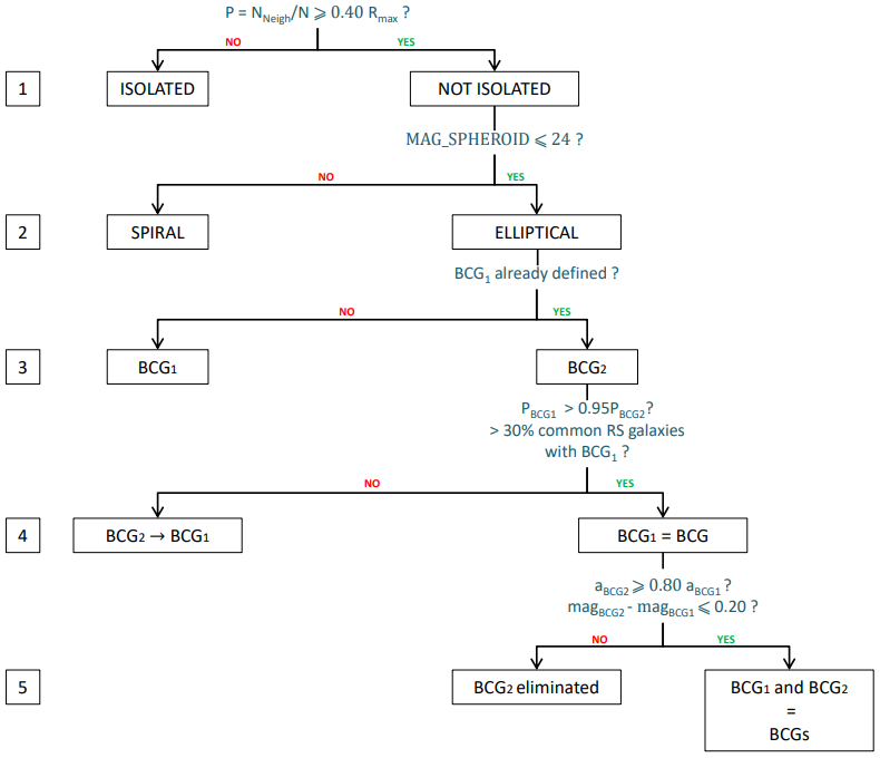
Figure 3: Flowchart showing how BCGs are automatically selected, in the case of a rich cluster (see description of the method for our definition of a rich cluster). Values may change for less rich clusters (see Section 3.1.3).

The method applied to select automatically red cluster BCGs is schematically summarized in Figure 3, and will be described in detail below. The efficiency of the method will be discussed in Section 3.1.4. Blue BCGs will be mentioned in Section 3.2.

3.1.1 Rejection of foreground sources

In order to differentiate the BCG from other objects in the field, we need to identify which objects are part of the cluster and which are not. We describe below step by step our method to detect the BCGs among all the contaminations (stars, foreground and background galaxies, artifacts) in our images.

Measurements with SExtractor (refer to Bertin & Arnouts, 1996, for more details on the following mentioned parameters) were done using two different deblendings (parameters DEBLEND$\_$MINCOUNT = 0.01 and DEBLEND$\_$MINCOUNT = 0.02). The smallest deblending parameter, i.e, the finest deblending, is sufficient to separate two nearby galaxies without fragmenting excessively spiral galaxies in the foreground, and provides the most accurate measurements. However, BCGs can present a very diffuse and luminous halo which may be associated with intracluster light (ICL). We noticed that, in presence of nearby bright sources in the region of the BCG, SExtractor would detect only those foreground sources and process the BCG halo as a very luminous background. We therefore decided to run SExtractor in parallel with a coarser deblending to take this into account. The two catalogs obtained with two different deblending parameters are then matched: we keep the values obtained with the finer deblending, and add all new objects detected using a coarser deblending.

We compute the magnitude at which our catalogue is complete at 80%, m_80%. For this, we plot the histogram in apparent magnitudes and fit the distribution up to the magnitude at which the distribution drops. By dividing the number of detected sources by the total number of sources that is expected to be detected in a magnitude bin (given by the fit), we compute the completeness of the catalogue at each bin. We can then determine m_80%, and make a cut in apparent magnitude to reject all galaxies with m $\geq$ m_80% + 2, as the photometry will not be accurate for these faintest objects.

Our procedure to reject the various contaminations is as follows. First, we query in NED for all the sources in the region of the cluster and reject all those with a spectroscopic redshift that differs by more than 0.15 from the cluster redshift (—z - z_spec— $>$ 0.15). We identify bad detections by their magnitude values which get returned as MAG = 99.99 by SExtractor. All point sources or unresolved compact galaxies are eliminated using the parameter CLASS$\_$STAR $\geq$ 0.95 in SExtractor, which requires a PSF model to be fed into SExtractor, created with PSFex (Bertin, 2011). Most foreground galaxies can be identified by their excessively bright absolute magnitude when computed from their MAG_AUTO magnitude and assuming they are at the cluster redshift. We thus exclude all sources with an absolute magnitude MAG_ABS $\leq-26$.

We can identify edge-on spiral galaxies, which appear very elongated. They can be filtered by making cuts in elongation (defined in SExtractor as the ratio of the galaxy’s major to minor axis). As will be explained in Section 3.1.2, we consider two different filters. We define two different cuts depending on the filter we are looking at: in the bluest filter, we apply the criterion ELONGATION $\leq$ 2.3, and in the reddest filter, ELONGATION $\leq$ 2.6. The latter limit may seem quite high to filter efficiently all edge-on spiral galaxies. However, because of deblending issues, measuring with precision the lengths of the major and minor axes of the sources can be difficult, and will sometimes lead to a very elongated object. A very bright and elongated halo around the BCG, which can be linked to the ICL, will possibly return a high a/b axis ratio. This is the case for the BCG in RX J2129+0005, which has the highest a/b elongation (in the F606W filter) measured in our sample, reaching a/b=2.57 (see Figure 4). As the reddest filter is more sensitive to the ICL, we prefer to define a limit that is not too strict on this filter. It will not eliminate all edge-on galaxies (for that, we should lower the limit), but we cannot take the risk of filtering out any of the BCGs we are looking for. That’s why we define a different, stricter limit on the bluest filter, as it will be more sensitive to the blue stellar population present in the disk of spiral galaxies, and less to the ICL.

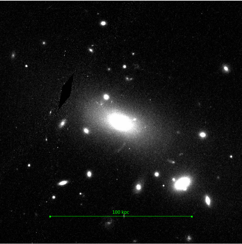
Figure 4: The BCG in RX J2129+0005 at redshift z = 0.234 has an extended and luminous halo, which makes it difficult to accurately estimate the a/b axis ratio. In this case, the major axis has most likely been overestimated, as the diffuse light is extended along this axis. The image was taken with the F775W ACS filter.

3.1.2 Selection of red cluster galaxies

Early-type galaxies in clusters are usually easily recognizable by their red colors, since they are mostly red elliptical galaxies, without star formation. While blue spiral galaxies also exist inside the cluster, they are a minority, and red elliptical galaxies draw a red sequence in a color-magnitude diagram, which has a low dispersion. We thus apply a filter in color in order to only keep the red galaxies that form the red sequence.

To extract all the red early-type galaxies in a cluster at redshift z, we model their color using a spectral energy distribution (SED) template from Bruzual & Charlot (2003). The model is similar to the one used by Hennig et al. (2017): a single period of star formation beginning at redshift z_f = 5, with a Chabrier IMF and solar metallicity, that decreases exponentially with $\tau=0.5$ Gyr. However, the model differs from Hennig et al. (2017) on the star formation redshift: we chose a higher z_f to better model clusters at higher redshifts, as Hennig et al. (2017) limit their study to redshift z = 1.1. We reject all blue galaxies (blue-red $\leq$ 0) and all galaxies whose measured (blue-red) color differs by more than 0.60 magnitude from the model. While the red sequence of a cluster presents a rather narrow color-magnitude relation, and therefore very little dispersion, this large limit of 0.60 was fixed in order to take into account photometric uncertainties due to deblending issues, redshift uncertainties, or simply to the accuracy of the model used (Charlot, private communication). The color is computed considering a fixed aperture of 35 kpc in diameter (parameter MAG_APER), which is large enough to contain all of the galaxy’s light. All magnitudes are K-corrected (K-correction values are taken from the EZGAL BC03 computed model) and we also take into account galactic extinction. Dust maps were taken from Schlegel et al. (1998) and reddening values for the ACS and WFC3 bandpasses were taken from Schlafly & Finkbeiner (2011), considering a reddening law R_V = 3.1. The color computed will depend on the filters available and on the redshift of the cluster. The colors computed for each cluster can be found in Table 1.

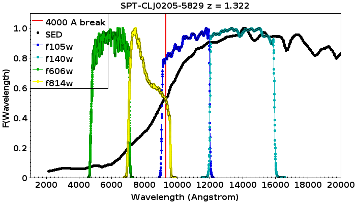
Figure 5: SED of an elliptical galaxy from the CFHTLS (black solid line) redshifted at the cluster’s redshift (SPT-CL J0295-5829, z = 1.322). The filter transmissions are normalized to 1 for better visualisation, and the break at 4000 Å is marked as a red vertical line for reference. In this case, the chosen (blue-red) rest frame color is F814W-F105W, and the filter we choose for the final step (modelisation of the luminosity profile with GALFIT) is F140W (see Section 4).

The rest frame (blue-red) color to compute is defined as the color based on two magnitudes with the smallest wavelength difference that bracket the 4000 Å break at the cluster redshift. Depending on what filters are available for each cluster, the selected filters will differ. An example is given in Figure 5, for a cluster at z = 1.322; in this case, the filters bracketing the 4000 Å break are F814W and F105W . In the cases where the two optimal filters are not available, the color used for tracing the red sequence galaxies at different redshifts may not be efficient; for instance, the use of the color (F606W - F140W) would not enable us to optimize the selection, as a galaxy at higher redshift (z = 1.65 for example) than the cluster redshift (here z = 1.322) would have the same color and will not be filtered out.

3.1.3 Rejection of spiral and isolated galaxies

The cut in colors is an important step that allows to remove most of the spiral galaxies and to maximize the number of ellipticals in our catalogues. However, a few foreground galaxies may still remain, and we describe here the method used to remove them.

The algorithm described hereafter will be applied to every single galaxy, from the brightest to the faintest, until the cluster BCG is found. We refer the reader to the sketch shown in Figure 3. The procedure includes the following steps:

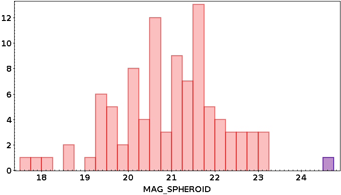
Figure 6: Histogram of the modeled bulge magnitudes (parameter MAG_SPHEROID) returned by SExtractor. All BCGs are shown in red, the blue point represents a spiral galaxy close to the cluster ClG J1604+4304 (see Step 2).

• Step 1: for each cluster, we sort the catalog from the brightest to the faintest galaxies, and going down their brightnesses, we exclude galaxies that are too isolated from the rest (explained hereafter). We define the BCG as the brightest elliptical galaxy at the center of the galaxy density distribution. The method to calculate the center is as follows:

  We compute N_neigh, the number of cluster members, i.e. red sequence galaxies, found in a fixed aperture of 200 kpc radius centered on each galaxy in the final catalogue, and note N_max the maximum number computed. If N is the total number of red sequence galaxies whose colors fall within 0.60 magnitude from the model, and N_neigh is the number of neighbours of a given galaxy in an aperture of 200 kpc, we consider that a galaxy is isolated and unlikely to be the BCG if the ratio P = N_neigh/N is smaller than 40$\%$ of P_max = N_max/N.

  Considering that we cropped our images to cover a projected area of 1.2x1.2 Mpc², the aperture of diameter 400 kpc taken here represents one third of the side of the images. This is small enough to detect high density areas on the image, and big enough to work on clusters with a high spatial extent. After several trials adopting different values, the value of 200 kpc radius is the one that works best. Less than 200 kpc becomes too small for extended clusters, while a higher radius makes it difficult to detect the smaller density fluctuations, as the covered area becomes large. The limit defined at R_lim = 0.40 R_max was also determined after several tests. This condition allows to take into account the cluster richness and spatial extent, as well as the possible offset of the BCG relatively to the cluster center.

• Step 2: the next step consists in filtering out the last spiral galaxies that remain among the potential BCG candidates. We run SExtractor to model the potential BCG with a bulge and a disk component. We find that spiral galaxies have a very faint bulge (parameter MAG_SPHEROID): as can be seen on Figure 6, a spiral galaxy (shown in blue) near the cluster ClG J1604+4304 prevented us from successfully detecting the BCG. We see a gap in magnitude between the spiral galaxy and the other BCGs (which are not all pure ellipticals). This enables us to define a new cut in magnitude to remove these remaining spirals: MAG_SPHEROID $\leq$ 24.

• Step 3: if a galaxy complies with these conditions, i.e. not being isolated and not being a spiral, we keep it as BCG₁ if no other BCG candidate was found before, and as BCG₂ otherwise. We don’t proceed to the next step until a BCG₂ is defined.

• Step 4: we check if there are more red sequence members in the same aperture for BCG₂ than the number defined in Step 1 for BCG₁, by comparing their P_Neigh ratios (defined in Step 1). We will note them P_BCG1 and P_BCG2. If P_BCG1 $\leq$ 0.95 P_BCG2, and if less than 30% of N_Neigh,BCG2 are in common with BCG₁, BCG₁ is eliminated and we define BCG₂ as the new BCG₁.

  The factor of 95% ensures that the overdensity in which BCG₂ resides is significantly richer than the one in which BCG₁ is. The second criterion on the number of common galaxies to BCG₁ and BCG₂ is to make sure that we are not replacing a BCG that is not at the very center of the cluster by another galaxy that is closer. This criterion is necessary to avoid eliminating BCGs that are a little offset from the center of the cluster, where the density is higher. It allows to check that the two galaxies are not in the same area in the sky, i.e, we check that BCG₂ does not belong to the same clump (overdensity) as BCG₁, or that the two galaxies do not belong to the same cluster.

• Step 5: this step is taken only if BCG₂ is defined, otherwise we repeat the previous steps until it is found. If BCG₁ and BCG₂ are similar in sizes (ratio of the major axes a_BCG2/a_BCG1 $\geq$ 0.80) and brightnesses (magnitude difference mag_BCG2 - mag_BCG1 $\leq$ 0.2), we keep both BCG₁ and BCG₂ as the BCGs of the cluster. Otherwise, BCG₂ is eliminated and BCG₁ is defined as the BCG.

The values above do not always work for poor clusters, i.e., when the number of cluster members is low, or when the density of red sequence galaxies is low. There is no problem when all the cluster members are concentrated in the same area (with a size comparable to the previously defined aperture), but if the members are dispersed over the sky and cover a large area, an aperture of 200 kpc radius becomes too small to detect density fluctuations on the sky. We thus differentiate these clusters by their number of red sequence members, N, and by the previously defined parameter P_max (see Step 1). We separate the poor clusters with P${}_{max}\leq$ 0.25 and N $\leq$ 100 (very extended cluster with no important density clumps), and P${}_{max}\leq$ 0.5 and N $\leq$ 40 (low number of red sequence galaxies, extended spatial distribution). We were not able to correctly determine the BCGs for these clusters by defining a 200-kpc radius aperture, so for these poorer clusters, we consider a bigger aperture of 500 kpc radius. To take into account the bigger aperture, we also modify the second criterion in Step 4. We check that the two BCGs candidates, BCG₁ and BCG₂, have less than 50% galaxies in common in the same aperture, to guarantee that they are not both residing in the same cluster.

3.1.4 Results for detected red BCGs

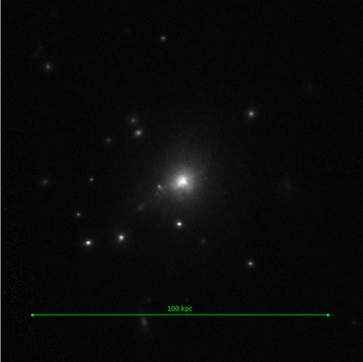
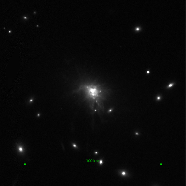
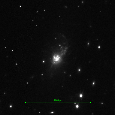
Figure 7: From left to right: MACS J0329-0211 (z = 0.45): an example of a red star forming BCG, RX J1532+3020 (z = 0.3615),and MACS J1932-2635 (z = 0.352): the only two blue star forming BCGs in our sample.

Among the 137 clusters in our sample, 50 clusters only had one filter available, and were thus excluded from this procedure. For these 50 clusters without available colors, we checked visually the images to determine the BCG, and checked with X-ray maps or other studies before adding them to the final sample.

In order to assess the efficiency and accuracy of our detection method, we checked each detection visually and compared it with other studies and with any X-ray map we could find. We compared the X-ray map to the position of the detected BCG to make sure that it is not too far from the X-ray peak (but not necessarily located at the peak, in a radius of about 200 kpc).

During this verification, we found that our detection differs from that of Durret et al. (2019) and Bai et al. (2014) for the BCGs in MACS-J0717.5+3745 and SpARCS-J0224 respectively. MACS-J0717.5+3745 presents a very complex structure as is it undergoing multiple mergers (see Limousin et al., 2016; Ellien et al., 2019, and references therein). Durret et al. (2019) define the BCG as the one in the southern structure, whereas we detect a brighter galaxy in the northern structure, that we hence define as the BCG. We choose to keep our detection as it lies near the X-ray peak in the northern structure and is surrounded by galaxies at the cluster’s redshift. We find, by checking visually, that the BCG in SpARCS-J0224 defined in Bai et al. (2014) is a spiral galaxy. We thus choose to keep our detection, which is an elliptical galaxy located just south of their detection.

A few star forming BCGs can be found in our sample. We find red BCGs with a very high SFR: we give the example of MACS J0329.6-0211 at z = 0.45. This BCG has an almost starburst level of UV continuum and star formation (Donahue et al., 2015). Images of this BCG in the UV continuum and H$\alpha$-[NII] lines are given by Fogarty et al. (2015), illustrating the distribution of star formation throughout the galaxy. The high star formation rate of about 40 M_⊙ yr^-1 was confirmed by Fogarty et al. (2017), based on Herschel data. Green et al. (2016) also indicate that this galaxy hosts an AGN, and is quite blue ($blue-red=-0.71$), with strong emission lines and a rather high X-ray luminosity of $11.85\times 10^{44}$ erg s^-1.

Overall, all the red BCGs, even the non pure elliptical BCGs, or those with not optimized colors because of the lack of available filters, were successfully detected with our method. We successfully detect 97% of the BCGs in our sample, and all the red BCGs are found. The method is effective to detect red BCGs presenting different morphologies and characteristics (mergers, star forming, traces of dust in the core, disturbed).

It is to note, though, that this method may be less reliable for poorer clusters (as defined in the previous subsection). As we were conducting several tests, trying different values of apertures in which we computed the number of red sequence galaxies, or the threshold below which galaxies are considered as isolated, we found that the detection efficiency for poorer clusters was more sensitive to these parameters. As this method relies on the density of red sequence galaxies in a small aperture, BCGs that are a little offset from the density peak (which is more difficult to calculate for poor clusters with an extended spatial distribution) could be eliminated, and rejected as being isolated from the other red sequence galaxies.

It may also be important to note that, in the presence of more than one cluster, i.e. two clusters interacting with each other, or in the case of superclusters, only the brightest galaxy of one substructure will be detected. For MACS-J0717.5+3745 for example, which we already mentioned, the BCG of the northern clump being the brightest, it is the one that is detected by our algorithm.

3.2 Finding blue BCGs

Out of the 98 BCGs (87 clusters, 11 clusters with two BCGs) in our sample which we tried to detect, we find two peculiar BCGs with blue colors.

BCGs are in majority quiescent galaxies, and their dominant stellar population is typically red and old. As they grow by undergoing mergers through time, all their gas is consumed, and we expect the star formation to be quenched or suppressed. However, we do observe, both today and in the distant universe, BCGs with intense UV emitting filaments or knots, hinting at active star formation. Cerulo et al. (2019) found that 9% of his sample of massive BCGs in the redshift range 0.05 $\leq$ z $\leq$ 0.35 from the SDSS and WISE surveys have blue colors (which they define as galaxies with colors $2\sigma$ bluer than the median color of the cluster red sequence), and are star forming. What we will refer to from now on as star forming BCGs (SF BCGs) have only been observed in cool core clusters so far. Their morphology can be quite different from that of a simple elliptical galaxy, as was stated before. These galaxies can appear disturbed, with a complex structure showing a possible recent or ongoing merger. Such examples of SF BCGs show that BCGs are not all simple ellipticals.

Two BCGs, RX J1532+3020 (z = 0.3615) and MACS J1932-2635 (z = 0.352), were not correctly detected as they are cool core BCGs with an extremely active star forming center, so they were eliminated because of their blue colors. These two BCGs were identified by eye and added manually, after checking and confirming with other studies. Their images are shown in Figure 7.

These two BCGs are the only blue BCGs in our sample (blue meaning a negative rest frame blue-red color), out of the 98 BCGs for which we compute a color. While comparing with other studies, we find a few other BCGs that are star forming, but are still red.

RX J1532+3020 is one of the most extreme cool core galaxy clusters observed today, as well as one of the most massive. An intensive study by Hlavacek-Larrondo et al. (2013) shows the existence of a western and an eastern cavity, which are used to quantify the AGN feedback at the center of the galaxy. These authors estimated that this feedback would release at least 10⁴⁵ erg s^-1, which would prevent the Intra Cluster Medium (ICM) from cooling, and would then allow to solve the cooling flow problem in cool core clusters. The BCG of this cluster is a radio loud galaxy that presents in its central regions UV filaments and knots, as well as traces of dust, hinting at recent star formation, with a SFR of at least 100 M_⊙ yr^-1 (Castignani et al., 2020). A strong and broad Lyman $\alpha$ emission and stellar UV continuum, and no other emission lines, have been observed by Donahue et al. (2016). CO with a large reservoir of molecular gas as well as a high level of excitation were also detected by Castignani et al. (2020).

MACS J1932-2635 is another cool core cluster with a huge reservoir of cold gas in the core, of mass (1.9$\pm$ 0.3) $\times$ 10¹⁰ M_⊙, which makes it one of the largest reservoirs observed today, in which Fogarty et al. (2019) detected CO emission as well as UV knots and H$\alpha$ filaments around the BCG. They measured a SFR of 250 M_⊙ yr^-1 and also observed an elongated tail that extends to the northwest, with traces of cold dust in the tail, which they suspect might be caused by a recent AGN outburst.

In order to detect these blue BCGs, we would have to relax the condition on the color. However, this condition is necessary in order to remove most of the spiral galaxies, and we find that allowing galaxies with blue colors will make the method much less reliable, as the red sequence will be ill-defined. Our method is thus only reliable to detect red BCGs, even if they are not pure ellipticals (star forming or merging galaxies for example).

4 Luminosity profiles

We fit 2D analytical models on sources with GALFIT (Peng et al., 2002). Once the BCG is defined, we run SExtractor one last time to return model fit parameters in the available filter closest to the F606W rest frame at redshift z (see Figure 5), which is at a wavelength above the 4000 Å break and thus is in the spectral region where we will get the highest flux. The chosen filters can be found in Table 1. We note that there are 37 BCGs out of the 149 for which HST data are not available in the F606W rest frame or redder. The reddest filter is either bluer than the 4000 Å break or contains it, which means that we are not only looking at the oldest, reddest star population, but at the youngest bluest stars as well. These BCGs are marked by blue squares in plots. The redshift distribution of all our BCGs is plotted in Figure 2, the blue histogram represents the clusters with filters which are bluer than the 4000 Å break. These clusters observed in too blue filters are mainly between redshifts 0.7 and 1.2.

4.1 Masking

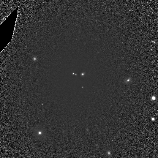
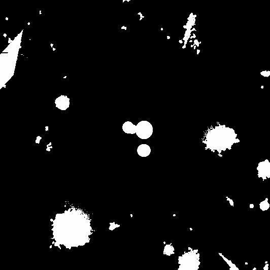
Figure 8: Example of the BCG in the cluster Abell 2261, at z = 0.224. (Left) The segmentation map returned by SExtractor, with the BCG unmasked. The pixels with a value of 1 are masked, those with a value of 0 are unmasked. (Middle) Sharp divided image, in which four knots in the core appear. These knots were drowned in the light of the BCG and are now visible. (Right) Final mask (including the central objects).

We first need to mask all the neighbouring sources. We take the SEGMENTATION map returned by SExtractor, and unmask the BCG (which is identified by an identification number), and also mask any blank region on the image. Because of deblending issues, it is more than likely that other objects, projected on the BCG, need to be masked.

We use sharp divided images to detect any neighbouring objects that pollute the signal. Sharp divided (SD) images (see e.g. Márquez et al., 1999, 2003) are obtained by dividing the images by the median filtered corresponding images. This brings out all the small neighbouring sources that may have been hidden by the luminous halo of the BCG. We run SExtractor (again) on this SD image, and mask all the objects that are farther than 0.5 arcsec from the BCG coordinates (an example is given in Figure 8), which is the minimum distance required to avoid masking the BCG center. As can be seen on Figure 8, the sources masked based on the SD image detection seem larger on the final mask than on the SD images, as the SD image does not show the true sizes of the objects. We apply a factor of 6 to the minor and major axes of the sources detected by SExtractor on the SD image to create our final mask. This factor allows to include all the luminosity of the sources and to mask them efficiently. If necessary, we identify by eye and draw the regions to be masked ourselves in SAOImage DS9 and create a new mask.

4.2 PSF model

To obtain a successful model of the galaxy profiles that also works for the inner regions, an accurate description of the PSF is needed. While the PSF we used for the photometry may have been sufficient to distinguish stars from galaxies, GALFIT requires the PSF to meet a number of criteria: a very high SNR, a flat and zero background (if not, any pattern in the background will appear on the model image when convolved with the PSF); it should match the image (diffraction rings and spikes, speckle pattern, etc.) and be correctly centered (see GALFIT Technical FAQ).

We first substract from the images the sky background, which is determined by masking all sources and blank areas on the cluster image, using the routine calc_background with a 3$\sigma$ clipping method. We then use PSFex, and make a selective sample of the stars that will go into making the PSF. We select all point-like sources with FLAGS = 0, MAG_AUTO $\leq$ 21, ELONGATION $\leq$ 1.1, CLASS_STAR $\geq$ 0.98, SNR $\geq$ 20 and an isophotal print ISOAREA_IMAGE $\geq$ 20 pixels.

Since we work on HST observations that cover a small field of view, there may not be many bright stars in the field of the cluster that we could use to compute a PSF. We tried to take several faint stars and stack them to increase the SNR of the PSF. However, we find that this often results in a PSF with an uneven background, which stands out during the model fitting returned by GALFIT, and this usually ends up being a bad fit (too large effective radius, large uncertainties). Since we are working on space observations, the PSF does not vary much, and though it may vary with time, the variations should not be significant (see Martinet et al., 2017). This means that we can replace the PSF for a given filter by another one in the same filter with a better SNR. Higher SNR PSFs return better fits.

Modeled and theoretical PSFs are available for ACS/WFC and WFC3/IR. However, according to GALFIT Technical FAQ (which we refer the reader to), the profiles obtained with models may not be realistic for space-based images, so we prefer to use observed PSFs.

4.3 Profile fitting

We use GALFIT to fit two different models to our BCGs: a single Sérsic component or two Sérsic components, to allow different contributions from the inner and outer parts of the galaxies. We also tried to apply other models or combinations of models including a de Vaucouleurs profile, but they always provided worse results (i.e. they gave a worse $\chi^{2}$, and about 30% of the BCGs were not well fitted with one or two de Vaucouleurs profiles), so we will only discuss the results with Sérsic fittings.

One needs to give GALFIT an estimate of all the initial parameters: the effective surface brightness or total magnitude, the effective radius (the radius at which half of the total light of the galaxy is contained), the elongation or the position angle (PA) of the BCG. These initial guesses are taken from the SExtractor catalogs: MU_EFF_MODEL or MAG_AUTO, FLUX_RADIUS, ELONGATION, and THETA_IMAGE. We don’t have an estimate of the BCG Sérsic index, so we start from the value corresponding to the de Vaucouleurs profile: n = 4. If the fitting does not converge, we try different Sérsic indices in the range 0.5 to 10. For the second Sérsic component that accounts for the inner part, the following parameters are considered: MU_EFF_SPHEROID, SPHEROID_REFF_IMAGE, SPHEROID_SERSICN and SPHEROID_THETA_IMAGE. The suffix SPHEROID refers to the bulb component when SExtractor tries to model a disk and a bulb to a galaxy. We consider an elongation (minor to major axis ratio, b/a) of 0.90 for the inner part, as an initial guess. The region to fit is a box that is 2.5 r_Kron wide (cf. GALFIT FAQ), r_Kron being the Kron radius returned by SExtractor. This is large enough to contain all the light from the BCG as well as some sky background, and is a good compromise to obtain good fits of our galaxies.

We first run GALFIT to fit the BCGs with one single Sérsic component. If it does not manage to converge with a Sérsic index of n = 4, we try different values between 0.5 and 10 until it converges to a meaningful fit, and reject any fit with returned effective radius larger than half the size of the fitting region, which is to say R${}_{e}\leq$ 2.5 r_Kron/2 pixels. We then use the output parameters as initial guesses to fit the outer part of the galaxy and add another Sérsic component to fit the inner part of the galaxy. If it does not converge towards meaningful values, we increment the Sérsic index until it manages to fit the BCG. For pairs of BCGs (two brightest cluster galaxies with similar sizes and magnitudes), we fit both of them simultaneously.

4.4 Choice of the best fit model

The quality of the fit can be estimated from the reduced $\chi^{2}$ ($\chi^{2}_{\nu}$), which should be close to 1. From our results, we notice that $\chi^{2}_{\nu}>$ 1.2 or $\chi^{2}_{\nu}<$ 0.8 often indicate a bad fit. This happens when the model used to fit the BCG is not adapted, or when the initial parameters given are bad estimates. In this case, GALFIT may also not have converged and/or crashed.

To decide if a second component is really necessary to fit the BCG, or if one component gives equally good results, we use the F-test (Simard et al., 2011; Margalef-Bentabol et al., 2016).

As stated in Bai et al. (2014), as the background noise is not gaussian, the meaning of $\chi^{2}_{\nu}$ is not as significant, and when comparing two models, a $\chi^{2}_{\nu}$ closer to unity does not necessarily mean that it is a better fit. So we prefer to use a F-test.

The F-test states that if the P-value, determined from the F-value and the number of degrees of freedom, is lower than a probability P₀, then you can reject the null hypothesis and consider that the second model gives a significantly better result than the simpler one. The F-value is defined as the ratio of the reduced $\chi^{2}$, $\chi^{2}_{\nu}$, of both models. GALFIT returns the $\chi^{2}$ as well as the $\chi^{2}_{\nu}$ of the fit, but instead of directly considering the output $\chi^{2}_{\nu}$ computed by GALFIT, we compute $\chi^{2}_{\nu}$ as:

$$\chi^{2}_{\nu}=\frac{\chi^{2}}{n_{dof}}$$ (1)

with n_dof the number of degrees of freedom, which is here defined as the number of resolution elements, n_res, minus the number of free parameters in the model, n_free. n_res can be calculated as follows (see Simard et al., 2011; Margalef-Bentabol et al., 2016):

$$n_{res}=\frac{n_{pixels}}{\pi\theta^{2}}$$ (2)

where $n_{pixels}$ is the number of unmasked pixels used for the fitting, and $\theta$ is the full width at half maximum (FWHM) of the given PSF, in units of pixels. $n_{dof}$ is then:

$$n_{dof}=n_{res}-n_{free}-1$$ (3)

The P-value is then calculated with the routine f.cdf from scipy.stats in python. We set $P_{0}=0.32$, which represents a $1\sigma$ threshold value (Margalef private communication).

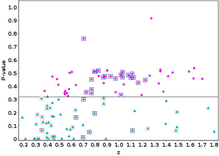
Figure 9: Distribution of P-values as a function of redshift considering a model with one Sérsic component (magenta), and a model with two Sérsic components (cyan). BCGs which could not be fitted by either model are not included.

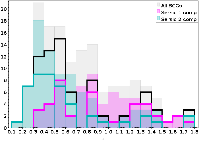
Figure 10: Distribution of redshifts for each model: a single Sérsic component (magenta) and two Sérsic components (cyan). In grey is represented the overall distribution. The semi-filled histograms represent the initial sample, and the unfilled histograms only contain BCGs with appropriate data.

We show the distribution of P-values as a function of redshift in Figure 9. A P-value $\leq$ P₀ means that we need a second component to correctly model the BCG light distribution. On this plot are not represented BCGs which could not be fitted by either model: 9 BCGs could only be fitted with a single component, 22 could only be fitted with two components, 2 could only be fitted by fixing the Sérsic index n = 4 (de Vaucouleurs profile), and 2 BCGs could not be fitted or returned a poor fit for either of the models. On Figure 10, it appears that BCGs that need a second component to obtain a good fit tend to be at lower redshifts (peak at z = 0.3), while the distribution for those that were well fitted with a single component is flatter. We also find BCGs with a model with two Sérsic profiles at higher redshifts (14 BCGs at z $\geq$ 1.0). If the chosen model depended on the distance, we would have expected not to have two component BCGs at higher z, which is not the case.

We must remember that part of our sample (37 BCGs) is studied in a too blue rest frame filter, and for these clusters we are not looking at the same star population. Without taking into account those observed in too blue filters, we find that 55 out of 72 BCGs (76%) at redshift z $\leq$ 0.8 need a second component, while the trend is reversed at z $>$ 0.8, as 23 out of 38 BCGs (61%) can be well modeled with only one component. We also notice that the BCGs observed with too blue filters can in majority (62%) be modeled with only one Sérsic.

We can also wonder if the existence of these two distinct populations (BCGs with two components at low z, and BCGs with a single component throughout redshift), with a limit around redshift z = 0.8, may be due to the fact that BCGs at higher redshifts will be less resolved than their lower redshift counterparts.

To test this hypothesis, we bring a sample of 44 BCGs at redshifts z $\leq$ 1.0 to a common physical scale at redshift z = 1.2. We smooth the images with a gaussian and repeat the previous steps. The $\sigma_{gauss}$ of the gaussian to apply is calculated as :

$\sigma_{gauss}$ = sqrt($\sigma_{z=1.2}^{2}-\sigma_{z,cluster}^{2})$ with $\sigma_{z,cluster}$ computed from the FWHM of the image we want to degrade, and $\sigma_{z=1.2}$ the $\sigma$ at the reference redshift z = 1.2, which was computed as:

$\sigma_{z=1.2}$ = $\sigma_{z,cluster}$ * $\frac{pixscale_{z=1.2}}{pixscale_{z,cluster}}$

Ouf of the 44 BCGs at z $\leq$ 1.0 on which we did this test, 30 returned similar results as those obtained with the original (unsmoothed) images. We also find that a few BCGs (seven) which were better fitted with two Sérsic components can be modeled just as well, according to the F-test, with only one Sérsic after smoothing the images. Surprisingly, the opposite also happened for seven other BCGs: among these seven BCGs, four could not initially be fitted with two components while the other three are close to the P-value limit, P_lim = 0.32. As 68% of the tested BCGs showed no significant difference, we can confirm that the lack of resolution for the farthest BCGs does not cause the absence of an inner component for BCGs at higher redshifts.

4.5 BCGs observed in too blue filters

In all that follows, when considering together the results from BCGs better fit with one or two Sérsic components, we consider the values obtained for the outer Sérsic component (R${}_{e,out}\geq$ R_e,in).

As stated before, we have 37 BCGs observed in too blue filters (relatively to the 4000 Å break). We must determine if they can be taken into account in our final study. For this, we run a test on 40 clusters with filters available on the blue side of the 4000 Å break as well as appropriate red filters, to check if the returned parameters vary depending on the filters chosen. We find that the absolute magnitude and mean effective surface brightness become fainter as the filter gets bluer. However, the dispersion is too big to simply correct for the offset to bring the BCGs observed in too blue filters to the appropriate red ones. This could be due to the fact that the filters on the blue side of the break do not always fall on the same spectral region on the SED (as the SED varies with redshift, and not all clusters were observed with the same filters). The effective radii can have their sizes halved when observed with too blue filters. As for the Sérsic indices, we find that the BCGs that need a second component tend to have Sérsic indices in bluer filters consistent with those measured in the appropriate red filters. The BCGs which could be fitted with only one Sérsic have indices that vary without any clear pattern. These observations show that we cannot directly consider together the measurements obtained looking at different parts of the SED. Therefore, we chose to exclude the BCGs observed in too blue filters in what follows.

We do however find that the position angles (PA) of the BCGs are not affected and remain consistent regardless of the filter chosen (see Figure 11). The PAs of these BCGs will thus be kept. Only one point presents a big difference between the two values (PA_red - PA_blue $>$ 120 degrees). We found that the ICL associated with this BCG is more extended in the reddest filter (Ellien et al., 2019, also show that the ICL tends to be more extended in redder filters). The other BCGs with a significant difference between the values measured in the two different filters are circular in shape (b/a $>$ 0.80), so the PAs are ill-defined, which also explains the huge error bars.

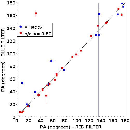
Figure 11: Difference between the PA measured on the appropriate red filter (x-axis), and the one measured in a too blue filter (y-axis). In red are BCGs with elongations b/a $\leq$ 0.80.

5 Results

As explained above, we tried fitting the BCGs with one or two Sérsic profiles. In the following, the values plotted are those from the best model determined using the F-test (see previous section). The resulting parameters are summarized in Table 2 and Table 3.

Two BCGs were not properly fitted by either model, but were correctly fitted by fixing the Sérsic index n = 4 (corresponding to a de Vaucouleurs profile). We thus kept the parameters obtained with this fit. Two other BCGs were not correctly fitted by either model, and are thus excluded, bringing our sample size to 147 BCGs.

We summarize the total numbers of galaxies that were better fit with each model:

• Sérsic (1 component): 63 BCGs

• Sérsic + Sérsic (2 components): 84 BCGs

Without taking into account the BCGs observed in too blue filters we have:

• Sérsic (1 component): 40 BCGs

• Sérsic + Sérsic (2 components): 70 BCGs

In all the plots shown in this paper, the BCGs better fitted with two Sérsic components will be represented with triangles, and those fitted with only one component with diamonds.

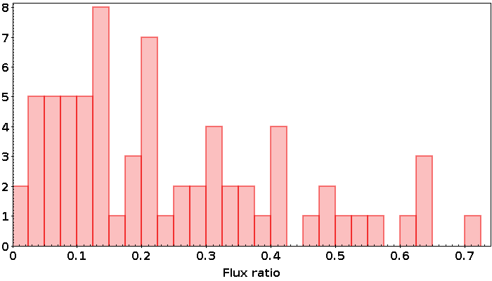
Figure 12: Histogram of the ratio of the flux of the inner component to the total flux of the BCG, for clusters better fit with two components. Clusters observed in too blue filters are excluded in this plot.

Before drawing conclusions, we need to know if we can consider together the results from BCGs better fit with one and with two Sérsic components. In principle, the two subsamples can be put together if, for the two components, we assume that the outer component contains most of the light of the BCG and that the outer profile represents well enough the overall luminosity of the galaxy. The more important the contribution of the inner component to the total luminosity of the BCG is, the less accurate this statement will be. If an inner component is required to model the BCG, then the resulting outer profile obtained when fitting two components may not be comparable to a profile obtained with only one component.

We show the histogram of the ratio of the inner component to total fluxes for the 70 BCGs requiring two Sérsic components (see Figure 12), and find that 24 BCGs present a very important inner component, which can contribute up to 30% of the total luminosity of the galaxy. If we choose to ignore these 24 BCGs, no obvious difference can be seen in the overall relations observed in the following. However, we prefer to exclude them, as the outer profile may not be comparable to the profile obtained with a single component modeling most of the light of the galaxy.

After excluding the galaxies with a very bright inner component and those observed in too blue filters, we obtain the final numbers:

• Sérsic (1 component): 40 BCGs

• Sérsic + Sérsic (2 components): 46 BCGs

In the following plots, BCGs observed in too blue filters will be marked with blue squares, and those fit with two Sérsic profiles and with an important inner component will be marked with light pink squares. We will also identify the blue SF BCGs (cf. Section 3) with red squares and pairs of BCGs with black triangles.

5.1 Evolution with redshift

In order to study the evolution of the BCGs, we consider the dependence of the derived parameters as a function of redshift.

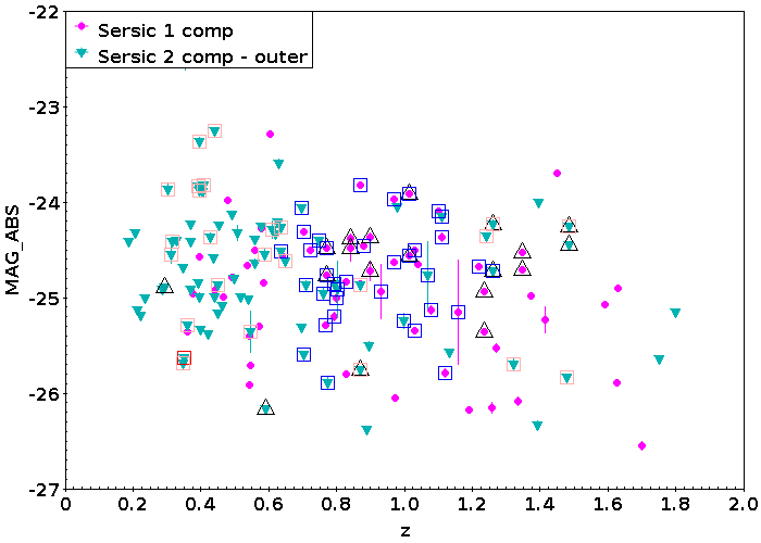
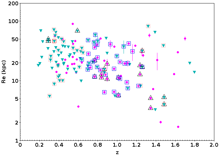
Figure 13: (Left) Absolute magnitude and (Right) effective radius in logarithmic scale as a function of redshift. Cyan triangles are BCGs fit by two Sérsic components (the outer component is considered), while the magenta points are BCGs fit with only one Sérsic component. Blue squares represent the BCGs observed in too blue filters, red squares are SF BCGs (see Section 3), black triangles are pairs of BCGs, and the light pink squares are BCGs with an important inner component contribution.

The absolute magnitudes of the BCGs, computed from the total apparent magnitudes (see Table 1 for the filters considered) calculated by GALFIT, despite the very big dispersion (4 magnitudes thoughout redshift) tend to become brighter with redshift (see Figure 13, left). The trend is faint, and can be quantified with a coefficient correlation R = $-0.29$ and a p-value p = 0.006563 (calculated from the coefficient R and the number of data points N ). By taking a significance level of $\alpha$ = 0.05, we show that we can reject the null hypothesis (p $<\alpha$) and conclude that the trend is significant.

There is a moderate trend for BCGs to grow with time (Figure 13, right), as those with the smallest effective radii are at higher redshifts (z $\geq$ 1.2). The trend in logarithmic scale is quantified by a correlation coefficient R = $-0.40$, and with a p-value of p = 0.000142. BCGs observed in too blue filters generally have smaller effective radii than the others at a given redshift. Those with an important inner component contribution do not appear to occupy a special place in these relations.

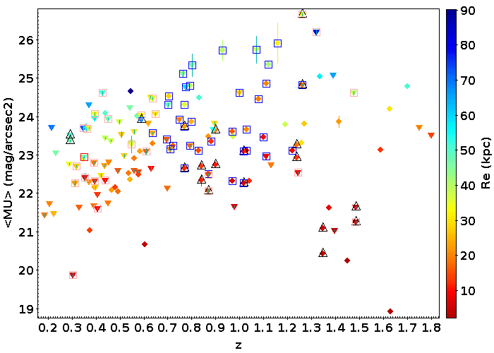
Figure 14: Mean effective surface brightness as a function of redshift. See Figure 13 for color code. Additional information on the effective radii of the BCGs is shown on the right of the figure.

The mean effective surface brightness (Figure 14) shows no significant evolution as a function of redshift (R $<<$ 0.1), with a very large dispersion (it spans a range of 6 magnitudes at z $\geq$ 1.25). Seven BCGs at higher redshifts (z $\geq$ 1.4) can be seen among the galaxies with the brightest mean effective surface brightnesses ($<\mu>\leq$ 22 mag arcsec^-2). We confirm that nothing peculiar was observed with these BCGs. Those observed in too blue filters and those with an important inner component contribution do not occupy a specific place in the relation.

The vertical gradient in color in Figure 14 shows that the large dispersion is also linked to the effective radius. As we go towards the biggest BCGs (increasing effective radii), the relation is shifted towards the fainter mean effective surface brightnesses. This is to be linked with the Kormendy relation, which will be shown in Section 5.2.

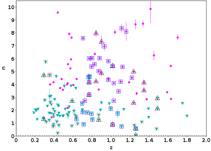
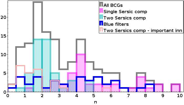
Figure 15: (Left) Sérsic indices as a function of redshift, see Figure 13 for color code. (Right) Distribution of the Sérsic indices. All BCGs are represented in the grey histogram. The magenta and cyan histograms represent the distributions obtained with one and two components respectively, only for the BCGs with appropriate data. The blue and lighter pink histograms represent BCGs observed in too blue filters and with an important inner component, respectively.

Finally, there is no correlation between the Sérsic index and redshift (Figure 15, left). However, on the right panel, we notice two different populations: the BCGs that were modeled with only one component generally have high Sérsic indices with a strong peak at n_1comp,mean = 4 (without considering the BCGs observed in too blue filters), while the BCGs that were better modeled with two Sérsic components with lower Sérsic indices show a peak at n_2comp,mean = 2.0.

5.2 Kormendy relation

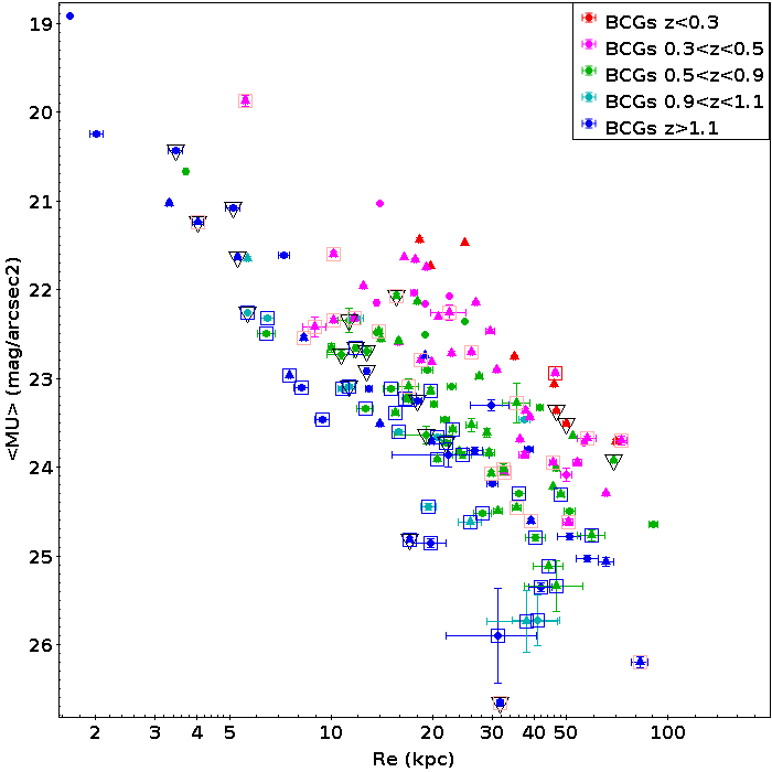
Figure 16: Kormendy relation (Kormendy, 1977) using the parameters obtained with one Sérsic component and the outer component of the two Sérsic component model. Different colors represent different redshift bins. Symbols are the same as in Figure 13.

The Kormendy relation (Kormendy, 1977) links the (mean) effective surface brightness of elliptical galaxies to their effective radius. This relation is plotted in Figure 16. The different colors represent different redshift bins: z $\leq$ 0.3, 0.3 $<$ z $\leq$ 0.5, 0.5 $<$ z $\leq$ 0.9, 0.9 $<$ z $\leq$ 1.3, and z $>$ 1.3. We show that all the BCGs seem to follow the Kormendy relation with the same slope, but the ordinate at the origin of the line decreases with increasing redshift.

While applying a linear regression to the relation obtained in each redshift bin (R $>$ 0.80, p $<\alpha$), we find that the slope remains quite constant at all redshift bins: m = 3.33 $\pm$ 0.73, whereas the ordinate at the origin varies as c = 2.15*z + 16.65.

5.3 Inner component

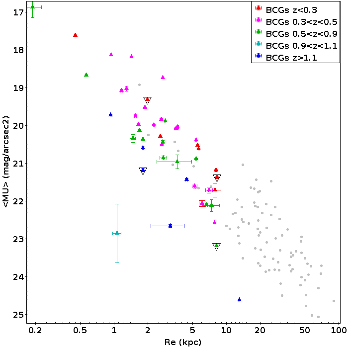
Figure 17: Same as Figure 16, but for the inner component of BCGs fitted with two components. Grey points are the same as in Figure 16.

The sample requiring an inner component consists of 46 BCGs. We find that the inner component follows a Kormendy relation (Figure 17), and is a continuation of the Kormendy relation shown in Figure 16 at brighter mean effective surface brightness and smaller effective radius (R${}_{e,inn}\leq$ 20 kpc).

We observe a very faint trend for the inner components to have brighter surface brightnesses with decreasing redshift, but the trend is not significant (R = 0.27, p = 0.06237 ¿ $\alpha$). We don’t find any clear correlation (correlation coefficient $\leq$ 0.2) between redshift and the absolute magnitude, effective radius or Sérsic indices of the inner component of the BCGs.

5.4 Alignment of the BCG with its host cluster

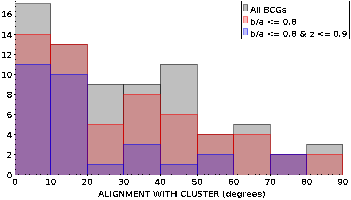
Figure 18: Difference between the PA of the cluster (see West et al., 2017; Durret et al., 2019) and that of the BCG as returned by GALFIT. Only clusters found in West et al. (2017) and Durret et al. (2019) are included here. The histogram is to be compared to that shown in West et al. (2017), as a way to check that our results agree with theirs. All BCGs are represented on the grey diagram, while only those with an axis ratio b/a $\leq$ 0.8 are included in the red diagram. We also exclude all BCGs at redshift z $>$ 0.9 on the blue histogram.

Some studies have shown that BCGs tend to have a similar orientation (hereafter PA) to that of their host cluster (West et al., 2017; Durret et al., 2019). As a comparison, we reproduce this study and compare our results with those of these two papers. The PA of the host clusters are taken from West et al. (2017) (computed from the moments of inertia of the distribution of red sequence galaxies) and Durret et al. (2019) (computed from density maps of red sequence galaxies), and the PAs of the BCGs are measured here with GALFIT. If measures are given in both papers, the PA_cluster in Durret et al. (2019) is taken, unless the PA_cluster is ill-defined (when the clusters are circular in shape), in which case the PA from West et al. (2017) is taken. We did not measure the PA of the host clusters for the clusters that are not presented in the above quoted papers, as our images are not large enough to accurately measure the full extent and shape of the cluster.

We include all BCGs for which the PA of the cluster was measured (73 BCGs), including those observed with too blue filters, as the PA measured by GALFIT is the same regardless of the filter (see Figure 11). We show the histogram of the alignment between the BCGs and their host clusters (defined as the difference of PA between that of the cluster and the BCG) in Figure 18.

We find that 39 BCGs (53% of the BCGs) are aligned with their host cluster with a difference smaller than 30 degrees. This already shows a tendency for BCGs to align with their host clusters, as a random orientation of the BCGs would result in a flat distribution. BCGs with the highest PA difference tend to be circular in shape (elongation = b/a $\approx$ 1, for which it is more difficult to measure a PA, resulting in high uncertainties). We thus chose to exclude all BCGs with axis ratio b/a $\geq$ 0.8, in order to eliminate BCGs with ill-defined PAs, as shown in red on the histogram. We then find that 32 out of 58 of BCGs are aligned with their host cluster within 30 degrees, slightly rising the percentage to 55%. There is a secondary peak between a PA difference of 30 to 40 degrees, mainly corresponding to BCGs at redshift z $\geq$ 0.9. At such high redshifts, galaxies appear smaller and therefore, the accuracy of the measured PA is probably worse. If we only consider galaxies at z $\leq$ 0.9 (blue histogram), we find that 22 BCGs out of 30 (73%) align with their cluster within less than 30 degrees. This shows that in majority BCGs tend to align with their host cluster at least at z $\leq$ 0.9.

5.5 BCG physical properties as a function of host cluster properties

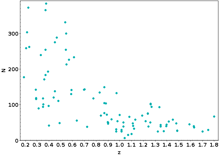
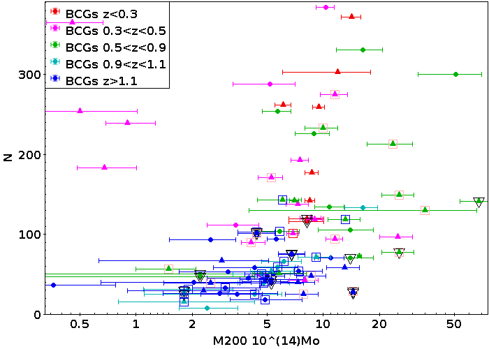
Figure 19: (Left) Richness of the cluster (see text) as a function of redshift. (Right) Richness of the cluster as a function of its mass M_200,c. The colors represent different redshift bins.

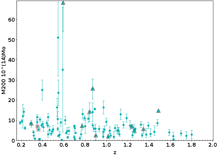
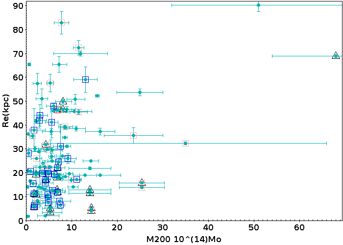
Figure 20: (Left) Cluster mass M200 (in units of 10${}^{14}M_{\odot}$ as a function of redshift. (Right) BCG effective radius as a function of cluster mass.

We browsed the available bibliography to retrieve the cluster masses and X-ray center coordinates. The corresponding data can be found in Table 4. We prefer lensing based mass estimates if available. We bring all the masses to M₂₀₀, applying the conversion factor between M₅₀₀ and M₂₀₀: M₅₀₀ = 0.72 M₂₀₀ (Pierpaoli et al., 2003).

We show the richness of the cluster as a function of redshift and cluster mass in Figure 19. The richness N of the cluster is defined here as the number of red sequence galaxies (found in Section 3) in an aperture of 500 kpc radius around the BCG. We obtain different values of N for two different BCGs in the same cluster because the richness is computed in an aperture centered on each BCG.

As can be seen on Figure 19 (left panel), clusters seem to become richer with decreasing redshift (correlation coefficient in logarithmic scale R = $-0.70$ and p-value of p $<$ 10^-5). Clusters at higher redshifts (z $\geq$ 1.0) have a lower richness, with a number of detected red sequence galaxies N $\leq$ 60. The right panel also shows that the most massive clusters are also the richest, and the high redshift clusters (blue points on the plot) with a low richness are also the less massive (M${}_{200,c}\leq$ 5 $\times$ 10¹⁴ M_⊙). This low value of N could in principle be due to the depth of our images, as we have a bias due to the distance: at higher redshifts, it is more difficult to detect objects and only the brightest ones can show up.

However, when looking at Figure 20, the left panel shows that we do not observe very massive clusters at high redshifts. So we have no bias due to the distance of the galaxies when measuring cluster masses: the masses are measured via lensing or derived from X-ray or SZ maps, which are independent of distance. Thus, we conclude that clusters become richer with time, and this result is not due to the depth of our images. However, although we only observe very massive clusters at lower redshifts (M${}_{200,c}\geq$ 30 $\times$ 10¹⁴ M_⊙ at z $\leq$ 0.8), the masses of the clusters do not vary much with time (R $<$ 0.20). The right panel shows that the very massive clusters only host bigger BCGs: cluster with masses M${}_{200,c}\geq$ 25 $\times$ 10¹⁴ M_⊙ only have BCGs with effective radii R${}_{e}\geq$ 30 kpc.

We find no correlations (R $\leq$ 0.2) between the BCG surface brightnesses or Sérsic indices and the cluster masses.

Using the relation given in Bai et al. (2014), we compute an estimate of the BCG masses from the cluster masses: M${}_{BCG}^{*}\propto$ M${}_{cluster}^{0.6}$. We find that the most massive BCGs are also the biggest in size (moderate correlation with R = 0.46 and p = 0.00007) and also tend to be brighter ($R=-0.32$, p = 007353). No correlation between the BCGs masses and redshift is seen (R $<$ 0.20).

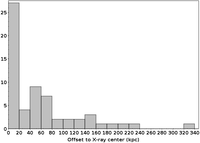
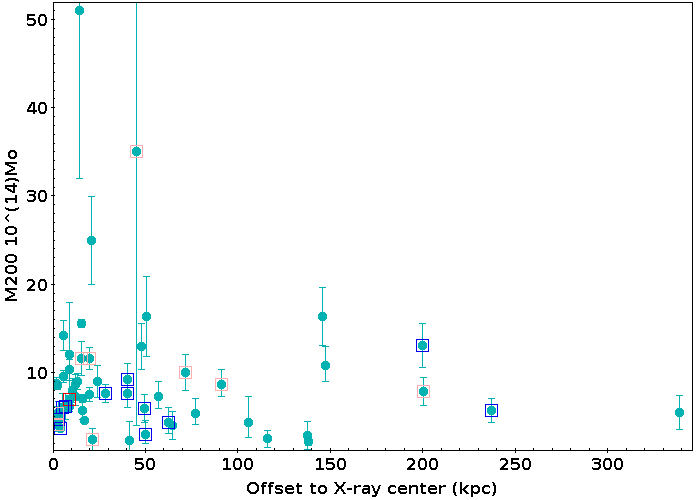
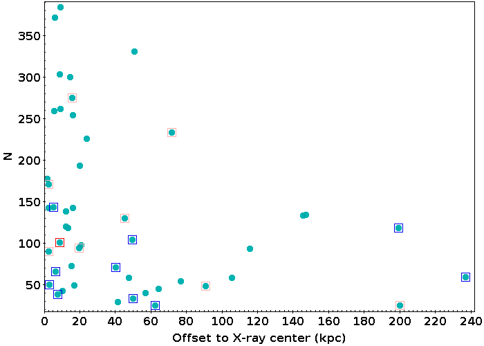
Figure 21: (Top left) Histogram of the offsets between the BCG and the X-ray center. As a function of the offsets between the BCG and the cluster X-ray center: (Top right) Masses M_200,c of the clusters (Bottom left) Richness of the cluster (Bottom right) Mean effective surface brightness of the BCGs.

We also study how the BCGs behave depending on their offsets to the cluster X-ray center. We exclude superclusters and clusters which present several substructures and/or several BCGs. We show the histogram of the offets on Figure 21, top left panel. We find that 31 out of 61 (51%) are within a 30 kpc radius range from the X-ray center of the cluster, showing that BCGs tend to lie close to the cluster X-ray centers. The two star forming BCGs that have undergone recent mergers and are not at equilibrium are also located at the center of the cluster (D_X $\leq$ 10 kpc). But, we confirm that there can be a significant offset between the two (12 out of 61 BCGs, 20%, present an offset bigger than 100 kpc). Although the corresponding plots are not shown here, we find no correlation between the offset and the absolute magnitude, effective radius, Sérsic index of the BCGs, or with the alignment previously computed.

As can be seen on the top right and bottom left panels of Figure 21, however, the more massive and the richer the cluster (or the BCG, as we converted the cluster masses to BCG masses), the closer the BCG is to the X-ray center of the cluster: the objects with the biggest offets ( $\geq$ 100 kpc) have masses M${}_{cluster}\leq$ 10 $\times$ 10¹⁴M_⊙ and richnesses N $\leq$ 100. We also find that there is a moderate correlation between the offset and the mean effective surface brightness of the BCG (see Figure 21, bottom right): BCGs tend to have brighter mean effective surface brightnesses the closer they are to the X-ray center (in logarithmic scale, R = 0.34, p = 0.0395).

We also analysed whether the most luminous BCGs are special (see Lin et al., 2010; Lauer et al., 2014). We studied the distribution of the difference in magnitude between the BCGs and the second ranked galaxies of the clusters. We found that the distribution was continue, with most BCGs having a difference smaller than one magnitude with the second ranked galaxy. By selecting BCGs which are at least brighter than 1 magnitude than the second ranked galaxy of the cluster (9 BCGs), we find that the most luminous BCGs do not occupy a specific place in the observed relations.

6 Discussion and conclusions

Our work deals with the largest sample (to our knowledge) of BCGs with HST imaging, covering a broad redshift interval from z = 0.1 to z = 1.8 (see Figure 1), and thus enabling us to trace the evolution of BCGs through time. Our sample is larger than most studies found in the literature based on HST images, such as Bai et al. (2014), DeMaio et al. (2019); Durret et al. (2019). We also study the luminosity profiles of these galaxies and how they evolve as a function of redshift. HST images allow us to perform profile fitting with precision, and GALFIT returns accurate parameters from model fitting.

We developed a new tool to detect automatically red BCGs on optical images. We successfully detected all the red BCGs regardless of their peculiar characteristics (see Section 3). We did not manage to detect in a similar way the blue BCGs, which represent here only 2% of our sample.

We then proceeded to model the luminosity profiles of these automatically detected BCGs, as well as those which have only one filter available, bringing this sample to 149 BCGs. We removed all BCGs observed in too blue filters as well as BCGs better modeled with two components for which the inner component has an important contribution to the total luminosity of the galaxy. Our final sample consists then of 86 BCGs.

We studied how the photometric properties of BCGs correlate with redshift, and we find that, although the correlation is weak -but significant, the absolute magnitude presents a faint trend to become brighter with time.

We show that there is a faint trend (see Figure 13, right) for BCGs to become bigger with decreasing redshift. This is the behaviour we expect for galaxies that grow in size with time, by accreting gas and merging with other smaller galaxies. This trend was also observed in Durret et al. (2019) up to redshift 0.9, and can be confirmed up to redshift z=1.8. Based on this relation, we find that BCGs grow by more than a factor 3 between redshifts 1.8 and 0.1. The dispersion can be linked with the Kormendy relation, that indicates that galaxies with higher surface brightnesses have smaller effective radii.

We find no strong correlation between the other photometric properties (surface brightness or Sérsic index) of the BCGs and redshift. This is in agreement with Bai et al. (2014) who do not find any correlation between the magnitude or the mean surface brightness of the BCGs and redshift, up to redshift z = 0.9. We add that no evolution can be observed up to redshift z = 1.8 either.

Although we do only observe massive clusters at lower redshifts (M${}_{200,c}\geq$ 30 $\times$ 10¹⁴ M_⊙ at z $\leq$ 0.8), overall, the masses of the clusters do not correlate with redshift. The growth of the cluster is mainly to be linked with the cluster richness (Figure 19): clusters become richer with time, and we find that the number of red sequence galaxies in an aperture of 500 kpc centered on the BCG increases by almost a factor 10 between z = 1.8 and z = 0.1. We confirmed that the low richness we measured at higher redshift is not due to the depth of our images. This growth mainly seems to be happening at z $\leq$ 1.0, as we do not observe a significant variation of the richness of the clusters before that time.

We use the relation found in Bai et al. (2014) to compute the BCG masses from the cluster masses, based on the relation found by Bai et al. (2014). We find that bigger BCGs are also more massive (see Figure 19): R${}_{e}\propto$ 4.42 $\times$ M_BCG, but the masses do not show a significant growth with redshift.

We thus find that the sizes of the BCGs grow faster than their masses in the same redshift range. Although we do not find that the masses of the BCGs grow significantly with time, whereas Bai et al. (2014) finds a factor 2 since z = 2, we agree that the sizes have grown significantly faster than the masses in the same redshift range. Bai et al. (2014) find that the sizes grow more than twice as fast as the masses. We confirm that the masses and sizes of BCGs do not grow at the same rate. This is in favor of a scenario in which BCGs grow thanks to minor dry mergers at the later stages of their formation and evolution. Indeed, a growth mainly due to major dry mergers would make the sizes and masses grow at the same rate.

To summarize, we can say that the sizes of the BCGs, as well as the richnesses of the clusters, evolve with redshift: clusters become richer with time and, at the same time, BCGs undergo dry mergers that increase their sizes.

Another interesting result is the distribution of Sérsic indices (see Figure 15) that shows two different populations with low Sérsic indices, mainly at low redshift (z $\leq$ 0.8) and high Sérsic indices. The limit is also to be linked to the fact that BCGs at lower redshifts often require a second component to correctly take into account the brighter core of the galaxy. We find that BCGs better modeled with two components have a peak Sérsic index n = 2, while those that were fit with a single component have a peak at n = 4. Those modeled with only one Sérsic component are thus comparable to pure elliptical galaxies which can be well modeled with a deVaucouleurs profile. This slightly differs from the results shown in Bai et al. (2014) who find a median value of n = 5.7. But, Bai et al. (2014) only fit a single Sérsic profile to all the BCGs in their sample. If we only look at the distribution we obtained for BCGs modeled with a single component, we find that this distribution is more comparable to that of ETGs shown in their paper. Another difference with that study is related to the filters chosen to model the luminosity profiles of the BCGs. While we consider the same spectral region of the SED for all clusters in order to only look at the same old red stellar population at all redshifts, Bai et al. (2014) observe all BCGs with the ACS F814W filter, which we find is already too blue for clusters at redshifts z $\geq$ 0.57. We also showed, by studying the parameters obtained in two different filters for a sample of BCGs, that the parameters will vary depending on the part of the SED you look at (when looking at a bluer filter, the absolute magnitude and mean effective surface brightness become fainter, the effective radius becomes smaller, and the Sérsic indices vary without any clear trend).

Finally, we find that the Kormendy relation (Kormendy, 1977) is also a function of redshift, with the relation shifted towards fainter mean effective surface brightnesses at higher redshifts. This relation shows that, at the effective radius, smaller galaxies are brighter and denser than the bigger ones. The slope of 3.33 $\pm$ 0.73 measured with our sample remains constant with redshift. Our value is in good agreement with that given in Bai et al. (2014):

¡$\mu$¿=(3.50$\pm$ 0.18)logR_e+(18.01$\pm$ 0.23)

and agrees within one $\sigma$ with the one given in Durret et al. (2019):

¡$\mu$¿=(2.64$\pm$ 0.35)logR_e+(19.7$\pm$ 0.5).

We should note that cosmology or selection effects might be contributing to the results in Figure 13, which shows a trend for BCG sizes and luminosities to increase with time. Despite its faintness, the contribution of the ICL should be taken into account. The ICL blends with the envelope of the BCG, making it difficult to differentiate the galaxy from the ICL, and this may affect our measurements (in particular those of the effective radii and Sérsic indices). The ICL might contribute at some level to measured sizes and luminosities of galaxies at low redshifts, yet might be missed in high-redshift clusters because of cosmological surface brightness dimming, or perhaps because the ICL has not yet developed in these young clusters. A concern comes from the value of the background, as GALFIT is sensitive to it, but its computation is limited by the sizes of the images (even without cropping).

We broaden the work by West et al. (2017) and Durret et al. (2019) on the alignment of BCGs with their host clusters. We removed BCGs with ill measured position angles due to their circular shape, as well as BCGs at higher redshifts, z $\geq$ 0.9, as they will appear smaller on the CCD, and will thus be less resolved and have less accurate measured PAs. This enables us to conclude that BCGs in majority tend to align with their host cluster at least at z $\leq$ 0.9, as after this selection 73% of the remaining BCGs are aligned with their host cluster within 30 degrees. This is a tighter alignment than that of Durret et al. (2019), who found an alignment for 12 out of 21 BCGs (57%) between redshifts 0.21 and 0.89. Okabe et al. (2020) study the alignment of 45 dark matter (DM) haloes and their BCGs up to z = 0.97, and find that BCGs tend to be well aligned with their DM haloes, with a mean difference of 22.2 $\pm$ 3.9 degrees. A similar study was done by Ragone-Figueroa et al. (2020) on the alignment of BCGs both with the distribution of cluster galaxies and DM haloes, by analyzing cosmological hydro-simulations of 24 clusters. They find a strong alignment at z $<$ 2, and add that relaxed clusters tend to host BCGs that align with their major axis. Similar conclusions are made by De Propris et al. (2020), who show that BCGs are generally aligned with their host cluster even when the offset between the BCG and the X-ray center is significant.

Cerulo et al. (2019) found that 9% the BCGs between 0.05 $\leq$ z $\leq$ 0.35 have colors bluer than $2\sigma$ of the median color of the cluster red sequence. During this study, we found two peculiar blue BCGs in our sample. Apart from their colors and complex structures, these two peculiar BCGs do not have photometric properties different from the other BCGs. It would be interesting to continue this study by considering a larger sample of SF blue BCGs, to see where they lie in the previous plots.

We plan to apply the method described in this paper to more than a thousand clusters from the CFHTLS, detected by Sarron et al. (2018), up to redshift z = 0.7. This will enable us to better evaluate the accuracy of our BCG detection method on ground-based-data, and although the resolution will not be as good, the sample will be significantly larger. We also found two BCGs (2%) with blue colors, and it would be interesting to estimate the fraction of blue BCGs in the Universe up to redshift z = 0.7. We can wonder if these BCGs evolve differently from the red BCGs that we detect.

Table 1: Sample of the 149 BCGs studied in this paper. The columns are: full cluster name, coordinates of the BCG, redshift, class of the BCG (if two BCGs are defined for a cluster, class 1 represents the brightest of the two), instrument, filter used to model the luminosity profile of the BCG (see Section 4), associated scale, color computed to extract the red sequence of the cluster (see Section 3). The BCGs with no values in the last column only had data in one filter, and their coordinates were taken from the literature.

Name	RABCG	DECBCG	Redshift	Class	Instrument	Filter	Scale	Color
	(J2000)	(J2000)					(kpc/″)
SPT-CLJ0000-5748	0.2504	-57.8093	0.702	1	ACS_WFC	F814W	7.128	F606W-F814W
Cl0016+1609	4.64	16.4378	0.5455	1	ACS_WFC	F850LP	2.83	F606W-F775W
SpARCS-J0335	8.9571	-43.2065	1.335	1	WFC3_IR	F140W	8.353	F105W-F140W
ACO2813	10.8528	-20.6282	0.2924	1	ACS_WFC	F814W	4.368	F435W-F606W
ACO2813	10.8548	-20.6169	0.2924	2	ACS_WFC	F814W	4.368	F435W-F606W
XDCPJ0044-2033	11.0236	-20.5651	1.59	1	WFC3_IR	F160W	8.42	F105W-F140W
RXJ0056-27	14.2374	-27.675	0.56	1	ACS_WFC	F814W	6.449
SPT-CLJ0102-4915	15.721	-49.2528	0.87	1	WFC3_IR	F105W	7.681	F625W-F775W
SPT-CLJ0102-4915	15.7409	-49.2719	0.87	2	ACS_WFC	F850LP	7.681	F625W-F775W
RXJ0110+19	17.5758	19.6387	0.317	1	ACS_WFC	F814W	4.617
Abell209	22.9689	-13.6112	0.206	1	ACS_WFC	F775W	3.373	F475W-F606W
CLJ0152-1357	28.1649	-13.9739	0.87	1	WFC3_IR	F105W	7.681	F775W-F850LP
CLJ015244.18-135715.84	28.182	-13.9552	0.84	2	WFC3_IR	F105W	7.598	F625W-F850LP
CLJ015244.18-135715.84	28.1824	-13.9555	0.84	1	WFC3_IR	F105W	7.598	F625W-F850LP
SPT-CLJ0205-5829	31.451	-58.4802	1.322	1	WFC3_IR	F140W	8.346	F814W-F105W
XMMXCSJ022045.1-032555.0	35.1895	-3.4333	0.33	1	WFC3_IR	F105W	4.743	F105W-F160W
RCSJ0220-0333	35.2316	-3.5633	1.03	1	ACS_WFC	F850LP	8.024	F775W-F850LP
RCSJ0221-0321	35.4299	-3.3542	1.016	1	ACS_WFC	F850LP	8.0	F775W-F850LP
RCSJ0221-0321	35.4369	-3.3678	1.016	2	ACS_WFC	F850LP	8.0	F775W-F850LP
XLSSJ0223-0436	35.7636	-4.6043	1.22	1	ACS_WFC	F850LP	8.269	F775W-F850LP
RCS0224-02	36.014	-2.471	0.408	1	ACS_WFC	F814W	5.425
SpARCS-J0224	36.1092	-3.3929	1.63	1	WFC3_IR	F160W	8.419	F105W-F140W
JKCS041	36.6815	-4.6894	1.8	1	WFC3_IR	F160W	8.39	F105W-F160W
Abell383	42.0141	-3.5292	0.1871	1	ACS_WFC	F775W	3.127	F475W-F606W
MACS0329-0211	52.4232	-2.1962	0.45	1	ACS_WFC	F850LP	5.745	F606W-F625W
SpARCS-J0330	52.733	-28.7166	1.626	1	WFC3_IR	F160W	8.42	F105W-F140W
RCS0337-2844	54.4539	-28.7517	1.1	1	ACS_WFC	F850LP	8.132	F775W-F850LP
RCS0350-08	57.6131	-8.9157	0.584	1	ACS_WFC	F814W	6.581
RCS0351-09	57.9159	-9.9406	0.304	1	ACS_WFC	F814W	4.487
MACSJ0416-2403	64.038	-24.0676	0.396	1	ACS_WFC	F850LP	5.328	F606W-F625W
MACS0429-0253	67.4001	-2.8851	0.399	1	ACS_WFC	F850LP	5.353	F606W-F625W
RCS0439-2904	69.9072	-29.0839	0.97	1	ACS_WFC	F850LP	7.913	F814W-F850LP
RCS0444-28	71.036	-28.3379	0.437	1	ACS_WFC	F814W	5.649
MACSJ0454.1-0300	73.5453	-3.0146	0.5377	1	ACS_WFC	F850LP	6.321	F775W-F850LP
RCS0511-42	77.8703	-42.5867	0.518	1	ACS_WFC	F814W	6.201
RCS0515-43	78.9047	-43.4207	0.44	1	ACS_WFC	F814W	5.672
RCS0518-43	79.6411	-43.4186	0.396	1	ACS_WFC	F814W	5.328
RCS0518-43	79.7313	-43.252	0.508	1	ACS_WFC	F814W	6.139
RCS0519-42	79.8316	-42.7978	0.603	1	ACS_WFC	F814W	6.679
RCS0519-44	79.9184	-44.0392	0.827	1	ACS_WFC	F814W	7.561
SPT-CLJ0533-5005	83.4035	-50.0957	0.881	1	ACS_WFC	F814W	7.709	F606W-F814W
SPT-CLJ0546-5345	86.657	-53.7586	1.16	1	ACS_WFC	F814W	8.207
SPT-CLJ0559-5249	89.9301	-52.8242	0.6112	1	ACS_WFC	F814W	6.721	F606W-F814W
SPT-CLJ0615-5746	93.9657	-57.7801	0.972	1	WFC3_IR	F125W	7.917	F814W-F105W
MACSJ0647+7015	101.9575	70.2488	0.5907	2	WFC3_IR	F105W	6.616	F625W-F775W
MACSJ0647+7015	101.961	70.2483	0.5907	1	WFC3_IR	F105W	6.616	F625W-F775W
MACSJ0717+3745	109.3985	37.7548	0.548	1	ACS_WFC	F850LP	6.381	F625W-F775W
MACSJ0744+3927	116.22	39.4574	0.6976	1	WFC3_IR	F105W	7.11	F606W-F775W
Abell611	120.2367	36.0566	0.288	1	ACS_WFC	F814W	4.322	F475W-F606W
RXJ0841+64	130.2818	64.3739	0.36	1	ACS_WFC	F814W	5.02
RXJ0847+34	131.7991	34.8144	0.56	1	ACS_WFC	F814W	6.449
RDCSJ0849+4452	132.2443	44.8659	1.261	2	ACS_WFC	F850LP	8.304	F775W-F850LP
RDCSJ0849+4452	132.2445	44.8658	1.261	1	ACS_WFC	F850LP	8.304	F775W-F850LP
RDCSJ0910+5422	137.6915	54.3687	1.11	1	ACS_WFC	F850LP	8.146	F775W-F850LP
RXJ0926+12	141.6529	12.7177	0.49186	1	ACS_WFC	F814W	6.034
RCS0928+36	142.0883	36.7744	0.393	1	ACS_WFC	F814W	5.303
Abell851	145.7417	46.9867	0.4069	1	ACS_WFC	F814W	5.416

Table 1: Continued.

Name	RABCG	DECBCG	Redshift	Class	Instrument	Filter	Scale	Color
	(J2000)	(J2000)					(kpc/″)
MOOJ1014+0038	153.5304	0.6408	1.27	1	WFC3_IR	F140W	8.31	F105W-F125W
LCDCS0110	159.4681	-12.747	0.5789	1	ACS_WFC	F814W	6.553
LCDCS0130	160.1678	-11.9345	0.7043	1	ACS_WFC	F814W	7.137
SpARCS-J1049	162.3441	56.6754	1.7	1	WFC3_IR	F160W	8.412	F105W-F160W
LCDCS0172	163.6016	-11.7722	0.6972	1	ACS_WFC	F814W	7.109
LCDCS0173	163.6813	-12.7645	0.7498	1	ACS_WFC	F814W	7.309
MS1054-0321	164.2496	-3.6265	0.83	1	ACS_WFC	F850LP	7.569	F775W-F850LP
RCS1102-03	165.6373	-3.318	0.423	1	ACS_WFC	F814W	5.543
RCS1102-05	165.7463	-5.3527	0.395	1	ACS_WFC	F814W	5.32
CLJ1103.7-1245	165.8957	-12.7798	0.63	1	ACS_WFC	F814W	6.812
RCS1104-04	166.1669	-4.7495	0.637	1	ACS_WFC	F814W	6.845
RCS1107-05	166.8505	-5.3862	0.794	1	ACS_WFC	F814W	7.459
RCS1107-05	166.9754	-5.2778	0.579	1	ACS_WFC	F814W	6.554
RCS1108-04	167.0611	-4.5142	0.638	1	ACS_WFC	F814W	6.85
MACSJ1115+0129	168.9662	1.4986	0.349	1	ACS_WFC	F850LP	4.921	F475W-F606W
SG1120-1202-2	170.0312	-12.0858	0.3704	1	WFC3_IR	F105W	5.112	F606W-F814W
SG1120-1202-1	170.0555	-11.9808	0.3707	1	WFC3_IR	F105W	5.114	F606W-F814W
SG1120-1202-3	170.0924	-12.0295	0.3713	1	WFC3_IR	F105W	5.119	F606W-F814W
RCS1122+24	170.6077	24.375	0.799	1	ACS_WFC	F814W	7.475
LCDCS0340	174.5423	-11.5607	0.4798	1	WFC3_IR	F105W	5.954	F814W-F105W
MOOJ1142+1527	175.6976	15.4531	1.19	1	WFC3_IR	F140W	8.24	F105W-F140W
MACSJ1149.5+2223	177.3987	22.3985	0.5444	1	ACS_WFC	F850LP	6.36	F625W-F775W
Abell1423	179.3223	33.611	0.2142	1	ACS_WFC	F775W	3.476	F475W-F606W
MACS1206-0847	181.5506	-8.8009	0.44	1	ACS_WFC	F850LP	5.672	F606W-F625W
LCDCS0504	184.1883	-12.0215	0.7943	1	ACS_WFC	F814W	7.46
CLJ1226+3332	186.7427	33.5468	0.89	1	WFC3_IR	F125W	7.732	F814W-F850LP
LCDCS0531	186.9953	-11.5872	0.6355	1	WFC3_IR	F105W	6.838	F814W-F105W
XMMUJ1229+0151	187.3721	1.8561	0.98	1	WFC3_IR	F105W	7.933	F775W-F850LP
LCDCS0541	188.1262	-12.8435	0.5414	1	ACS_WFC	F814W	6.342
RDCSJ1252-2927	193.2267	-29.4549	1.237	1	WFC3_IR	F125W	8.284	F775W-F850LP
RDCSJ1252-2927	193.2273	-29.4548	1.237	2	WFC3_IR	F125W	8.284	F775W-F850LP
MACSJ1311-0310	197.7577	-3.1777	0.49133	1	ACS_WFC	F850LP	6.031	F606W-F625W
RCS1319-02	199.8005	-2.1197	0.354	1	ACS_WFC	F814W	4.966
RCS1323+30	200.892	30.3802	0.46163	1	ACS_WFC	F814W	5.828
ZWCl1332.8+5043	203.5857	50.5177	0.62	1	ACS_WFC	F775W	6.764
RXJ1347-1145	206.8776	-11.7527	0.451	1	ACS_WFC	F850LP	5.752	F606W-F625W
LCDCS0853	208.5406	-12.5172	0.7627	1	ACS_WFC	F814W	7.355
RXJ1354-02	208.5716	-2.3664	0.54786	1	ACS_WFC	F814W	6.38
WARPSJ1415+3612	213.7962	36.2009	1.03	1	ACS_WFC	F850LP	8.024	F775W-F850LP
RCS1419+53	214.8006	53.4367	0.71	1	ACS_WFC	F814W	7.16
MACSJ1423+2404	215.9495	24.0784	0.5431	1	ACS_WFC	F850LP	6.352	F606W-F775W
IDCSJ1426.5+3508	216.6373	35.1399	1.75	1	WFC3_IR	F160W	3.734	F105W-F140W
ISCS1429+3437	217.3237	34.6207	1.258	1	WFC3_IR	F160W	8.301	F775W-F850LP
ISCSJ1432.3+3253	218.0757	32.8894	1.396	1	WFC3_IR	F140W	8.382	F105W-F140W
ISCSJ1432.4+3250	218.0947	32.8268	1.487	1	WFC3_IR	F160W	8.41	F814W-F160W
ISCSJ1432.4+3250	218.1038	32.8347	1.487	2	WFC3_IR	F160W	8.41	F814W-F160W
ISCSJ1432+3332	218.1137	33.5521	1.112	1	ACS_WFC	F850LP	8.148	F775W-F850LP
ISCSJ1432+3436	218.1574	34.6063	1.347	2	WFC3_IR	F160W	8.36	F850LP-F160W
ISCSJ1432+3436	218.1578	34.6084	1.347	1	WFC3_IR	F160W	8.36	F850LP-F160W
ISCSJ1434+3427	218.6255	34.4492	1.243	1	WFC3_IR	F125W	8.289	F850LP-F110W
ISCSJ1434.5+3519	218.6913	35.3314	1.373	1	WFC3_IR	F160W	8.373	F775W-F850LP
ISCSJ1438+3414	219.5352	34.2368	1.414	1	WFC3_IR	F160W	8.389	F850LP-F105W
RCS1446+08	221.7281	8.4512	0.628	1	ACS_WFC	F814W	6.803
MACSJ1447.4+0827	221.8584	8.4737	0.3755	1	ACS_WFC	F814W	5.156	F606W-F814W
RCS1450+08	222.6692	8.679	0.769	1	ACS_WFC	F814W	7.376
RCS1452+08	223.1133	8.5821	0.395	1	ACS_WFC	F814W	5.32
RCS1511+09	227.7654	9.0533	0.97	1	ACS_WFC	F850LP	7.913	F775W-F850LP
RXJ1532+3020	233.2241	30.3498	0.3615	1	ACS_WFC	F850LP	5.033	F606W-F625W
RXJ1540+14	235.2249	14.7655	0.44025	1	ACS_WFC	F814W	5.673
ClGJ1604+4304	241.1003	43.0772	0.9	2	ACS_WFC	F850LP	7.757	F814W-F850LP

Table 1: Continued.

Name	RABCG	DECBCG	Redshift	Class	Instrument	Filter	Scale	Color
	(J2000)	(J2000)					(kpc/″)
ClGJ1604+4304	241.1029	43.0741	0.9	1	ACS_WFC	F850LP	7.757	F814W-F850LP
RCS1620+29	245.0423	29.4901	0.8696	1	ACS_WFC	F814W	7.68
MACSJ1621.4+3810	245.3531	38.1691	0.465	1	WFC3_IR	F110W	5.852	F606W-F814W
OC02J1701+6412	255.348	64.2366	0.453	1	ACS_WFC	F814W	5.767
MACSJ1720+3536	260.0698	35.6073	0.3913	1	ACS_WFC	F850LP	5.289	F606W-F625W
Abell2261	260.6133	32.1325	0.224	1	ACS_WFC	F814W	3.597	F475W-F606W
MACSJ1932-2635	292.9567	-26.5756	0.352	1	ACS_WFC	F850LP	4.948	F606W-F625W
SPT-CLJ2040-5725	310.0551	-57.4208	0.93	1	ACS_WFC	F814W	7.827	F606W-F814W
SPT-CLJ2040-4451	310.2382	-44.8595	1.478	1	WFC3_IR	F160W	8.408	F105W-F140W
SPT-CLJ2043-5035	310.8233	-50.5923	0.723	1	ACS_WFC	F814W	7.21	F606W-F814W
SPT-CLJ2106-5844	316.5192	-58.7411	1.132	1	WFC3_IR	F140W	8.174	F814W-F105W
MACSJ2129-0741	322.3588	-7.691	0.5889	1	ACS_WFC	F850LP	6.606	F625W-F775W
RXJ2129+0005	322.4164	0.0892	0.234	1	ACS_WFC	F775W	3.717	F475W-F606W
MS2137-2353	325.0633	-23.6611	0.313	1	ACS_WFC	F814W	4.578	F475W-F625W
RCS2152-06	328.2013	-6.1599	0.649	1	ACS_WFC	F814W	6.901
RCS2156-0448	329.1759	-4.8013	1.07	1	ACS_WFC	F850LP	8.089	F775W-F850LP
XMMUJ2205-0159	331.4611	-1.9917	1.12	1	ACS_WFC	F850LP	8.159	F775W-F850LP
XMMXCSJ2215.9-1738	333.9973	-17.634	1.45	1	WFC3_IR	F160W	8.401	F850LP-F125W
XMMJ2235.3-2557	338.8369	-25.9611	1.393	1	WFC3_IR	F160W	8.381	F850LP-F105W
RCS2239-60	339.9784	-60.7457	0.429	1	ACS_WFC	F814W	5.589
RXJ2248-4431	342.1832	-44.5306	0.349	1	ACS_WFC	F850LP	4.921	F606W-F625W
RCS2316-00	349.2302	-0.1965	0.56	1	ACS_WFC	F814W	6.449
RCX2319+0038	349.9727	0.637	0.8972	1	ACS_WFC	F850LP	7.75	F775W-F850LP
RXJ2328+14	352.2178	14.8786	0.49885	1	ACS_WFC	F814W	6.08
SPT-CLJ2331-5051	352.9631	-50.865	0.5707	1	ACS_WFC	F814W	6.509	F606W-F814W
SPT-CLJ2337-5942	354.3653	-59.7014	0.775	1	ACS_WFC	F814W	7.397	F606W-F814W
SPT-CLJ2341-5119	355.3015	-51.3291	0.9983	1	ACS_WFC	F814W	7.968	F606W-F814W
RCS2342-35	355.5794	-35.5713	0.802	1	ACS_WFC	F814W	7.484
SPT-CLJ2342-5411	355.6913	-54.1848	1.08	1	ACS_WFC	F814W	8.104	F606W-F814W
RCS2345-3632	356.3729	-36.5461	1.04	1	WFC3_IR	F160W	8.041	F105W-F160W
SPT-CLJ2359-5009	359.9286	-50.1672	0.77	2	ACS_WFC	F814W	7.38
SPT-CLJ2359-5009	359.9326	-50.1723		1	ACS_WFC	F814W	7.38

Table 2: Parameters obtained from fitting the luminosity profiles of the BCGs with GALFIT. Only the parameters obtained for the chosen model are shown. If fitted by two Sérsic profiles, the parameters of the outer component are given (the parameters for the inner component are then given in Table 3). The columns are: full cluster name, class of the galaxy, best model (Sérsic being a model with a single component, Sérsic2 a model with two components, and Sérsic* by fixing the Sérsic index n = 4), absolute magnitude, mean effective surface brightness, effective radius, Sérsic index, elongation (ratio of the major to minor axis), position angle, alignment of the BCG with its host cluster.

Name	Class	Model	mABS	$<\mu_{e}>$	Re	n	b/a	PA	Alignment
			(mag)	(mag/arcsec2)	(kpc)			(degrees)	(degrees)
Cl0016+1609	1	Sérsic
SpARCS-J0335	1	Sérsic	-26.088	25.034	57.488	8.7	0.88	158	4
XDCPJ0044-2033	1	Sérsic	-25.073	23.119	12.944	3.39	0.36	11	63
CLJ0152-1357	1	Sérsic	-24.859	23.471	21.802	3.59	0.7	49
CLJ015244.18-135715.84	2	Sérsic	-24.378	22.698	12.74	4.24	0.75	42
CLJ015244.18-135715.84	1	Sérsic	-24.478	22.343	11.331	7.96	1.0	10
RCSJ0220-0333	1	Sérsic	-24.511	23.111	10.804	4.08	0.75	24	64
RCSJ0221-0321	1	Sérsic	-23.916	22.257	5.667	0.88	0.61	111	63
RCSJ0221-0321	2	Sérsic	-24.566	23.098	11.261	5.43	0.74	21	27
XLSSJ0223-0436	1	Sérsic	-24.675	23.103	8.146	4.52	0.74	47	69
SpARCS-J0224	1	Sérsic	-24.905	18.918	1.682	2.87	0.64	128
SpARCS-J0330	1	Sérsic	-25.891	24.187	30.167	5.43	0.67	9	34
RCS0337-2844	1	Sérsic	-24.102	23.468	9.433	4.21	0.72	114
RCS0350-08	1	Sérsic	-24.849	23.089	22.851	7.63	0.71	159
RCS0439-2904	1	Sérsic	-24.625	23.598	15.81	5.81	0.77	112
MACSJ0454.1-0300	1	Sérsic*	-24.66	22.513	19.069	4.0	0.74	119	31
RCS0515-43	1	Sérsic	-24.928	24.088	49.921	9.58	0.74	9
RCS0519-42	1	Sérsic	-23.293	20.669	3.71	3.95	0.81	112
RCS0519-44	1	Sérsic	-24.83	23.117	15.098	5.56	0.81	66
SPT-CLJ0533-5005	1	Sérsic	-24.463	23.344	12.609	6.03	0.76	149	72
SPT-CLJ0546-5345	1	Sérsic	-25.154	25.904	31.178	8.1	0.78	105	27
SPT-CLJ0615-5746	1	Sérsic	-26.055	23.471	37.3	4.46	0.66	19	49
RXJ0841+64	1	Sérsic*	-25.353	23.728	56.139	4.0	0.6	48
RDCSJ0910+5422	1	Sérsic	-24.369	24.853	19.696	8.36	0.78	18	13
MOOJ1014+0038	1	Sérsic	-25.528	23.814	26.754	3.3	0.68	52	13
LCDCS0130	1	Sérsic	-24.316	24.52	28.215	7.59	0.92	169
SpARCS-J1049	1	Sérsic	-26.55	24.782	51.065	7.63	0.94	85
MS1054-0321	1	Sérsic	-25.802	24.494	50.904	6.37	0.62	43
RCS1107-05	1	Sérsic	-25.196	24.795	40.238	5.37	0.65	66
RCS1107-05	1	Sérsic	-24.28	22.484	13.684	5.94	0.79	22
RCS1108-04	1	Sérsic	-24.563	23.294	20.204	4.42	0.48	98
RCS1122+24	1	Sérsic	-25.0	23.861	24.589	6.03	0.7	147
LCDCS0340	1	Sérsic	-23.979	22.153	13.621	4.41	0.74	92
MOOJ1142+1527	1	Sérsic	-26.175	23.799	38.599	4.16	0.66	76	4
MACSJ1149.5+2223	1	Sérsic	-25.909	24.645	90.254	4.1	0.71	131	12
RDCSJ1252-2927	1	Sérsic	-25.353	23.253	18.022	4.97	0.77	73	30
RDCSJ1252-2927	2	Sérsic	-24.943	22.918	12.784	2.57	0.73	66	23
MACSJ1311-0310	1	Sérsic	-24.793	22.043	17.613	3.57	0.86	132	34
RXJ1354-02	1	Sérsic	-25.709	23.334	41.547	5.57	0.77	20
WARPSJ1415+3612	1	Sérsic	-25.351	23.665	20.719	2.73	0.72	23	45
MACSJ1423+2404	1	Sérsic	-25.399	22.363	24.917	2.16	0.6	37	5
ISCS1429+3437	1	Sérsic	-26.15	23.308	29.892	8.65	0.93	58	28
ISCSJ1432+3436	2	Sérsic	-24.524	20.43	3.476	4.14	0.84	53
ISCSJ1432+3436	1	Sérsic	-24.714	21.079	5.116	3.53	0.88	31
ISCSJ1434.5+3519	1	Sérsic	-24.979	21.619	7.272	2.84	0.65	77	56
ISCSJ1438+3414	1	Sérsic	-25.233	23.866	22.274	9.86	0.78	36	81
MACSJ1447.4+0827	1	Sérsic	-24.961	21.031	13.976	1.45	0.54	86
RCS1450+08	1	Sérsic	-25.294	24.299	36.181	6.01	0.61	140
RCS1452+08	1	Sérsic	-24.575	22.162	19.019	4.15	0.92	11
RCS1511+09	1	Sérsic	-23.975	22.327	6.495	4.35	0.79	137	33
ClGJ1604+4304	2	Sérsic	-24.364	22.737	10.716	4.87	0.74	121
ClGJ1604+4304	1	Sérsic	-24.724	23.643	19.195	7.29	0.76	22
RCS1620+29	1	Sérsic	-23.819	22.501	6.405	5.03	0.78	93
MACSJ1621.4+3810	1	Sérsic	-24.991	22.075	22.448	3.72	0.77	129	4
SPT-CLJ2040-5725	1	Sérsic	-24.933	25.728	41.119	6.96	0.83	15	6
SPT-CLJ2043-5035	1	Sérsic	-24.501	23.233	16.648	2.74	0.67	111

Table 2: Continued.

Name	Class	Model	mABS	$<\mu_{e}>$	Re	n	b/a	PA	Alignment
			(mag)	(mag/arcsec2)	(kpc)			(degrees)	(degrees)
XMMUJ2205-0159	1	Sérsic	-25.794	25.354	42.005	5.36	0.64	18
XMMXCSJ2215.9-1738	1	Sérsic	-23.698	20.249	2.019	6.25	0.61	93	48
RCS2316-00	1	Sérsic	-24.509	22.908	19.319	7.9	0.91	71
SPT-CLJ2331-5051	1	Sérsic	-25.302	24.013	46.462	5.24	0.73	8	20
SPT-CLJ2342-5411	1	Sérsic	-25.128	24.448	19.462	3.45	0.68	7	42
RCS2345-3632	1	Sérsic	-24.659	22.317	11.956	8.04	0.75	28	56
SPT-CLJ2359-5009	2	Sérsic	-24.486	22.655	11.804	3.19	0.75	123	6
SPT-CLJ2359-5009	1	Sérsic	-24.766	23.726	21.984	4.15	0.69	123	6
SPT-CLJ0000-5748	1	Sérsic2	-25.601	24.306	47.94	1.85	0.53	162	8
ACO2813	1	Sérsic2	-24.891	23.516	49.81	4.7	0.72	175
ACO2813	2	Sérsic2	-24.894	23.362	46.464	1.3	0.53	148
RXJ0056-27	1	Sérsic2	-24.641	23.613	28.883	1.83	0.64	94
SPT-CLJ0102-4915	1	Sérsic2	-24.87	22.478	13.894	1.62	0.87	118	29
SPT-CLJ0102-4915	2	Sérsic2	-25.753	22.069	15.653	1.26	0.57	134	13
RXJ0110+19	1	Sérsic2	-24.411	22.709	26.043	1.1	0.72	44
Abell209	1	Sérsic2	-24.327	21.734	19.715	2.05	0.71	134	23
SPT-CLJ0205-5829	1	Sérsic2	-25.701	26.197	82.853	1.09	0.33	32	8
XMMXCSJ022045.1-032555.0	1	Sérsic2	-24.403	21.638	16.486	2.34	0.91	65
RCS0224-02	1	Sérsic2	-23.824	21.606	10.172	1.91	0.94	97
JKCS041	1	Sérsic2	-25.156	23.512	13.984	1.57	0.6	64	36
Abell383	1	Sérsic2	-24.417	21.437	18.34	1.82	0.84	17	1
MACS0329-0211	1	Sérsic2	-25.17	21.756	19.19	2.34	0.84	168	32
RCS0351-09	1	Sérsic2	-23.868	19.87	5.573	2.77	1.0	57
MACSJ0416-2403	1	Sérsic2	-24.997	23.951	53.747	0.92	0.4	50	15
MACS0429-0253	1	Sérsic2	-25.332	22.155	26.926	1.52	0.64	169	12
RCS0444-28	1	Sérsic2	-24.586	22.716	22.713	1.61	0.7	157
RCS0511-42	1	Sérsic2	-24.997	22.985	27.435	2.09	0.74	173
RCS0518-43	1	Sérsic2	-23.365	22.326	11.748	1.71	0.7	74
RCS0518-43	1	Sérsic2	-24.326	23.526	26.018	3.89	0.73	31
SPT-CLJ0559-5249	1	Sérsic2	-24.29	23.094	17.035	1.93	0.92	41	45
MACSJ0647+7015	2	Sérsic2	-26.169	23.921	68.842	2.7	0.46	109	24
MACSJ0647+7015	1	Sérsic2	-25.779	23.92	57.494	0.06	0.23	111	26
MACSJ0717+3745	1	Sérsic2	-25.353	23.278	35.644	1.58	0.66	66	4
MACSJ0744+3927	1	Sérsic2	-25.312	22.136	17.986	2.05	0.77	21	80
Abell611	1	Sérsic2	-24.919	22.756	34.895	1.4	0.61	43	14
RXJ0847+34	1	Sérsic2	-24.387	22.589	15.827	2.29	0.89	4
RDCSJ0849+4452	2	Sérsic2	-24.723	24.822	17.068	0.57	0.58	116	38
RDCSJ0849+4452	1	Sérsic2	-24.236	26.658	31.769	0.07	0.84	59	85
RXJ0926+12	1	Sérsic2	-24.127	22.596	15.816	1.56	0.59	66
RCS0928+36	1	Sérsic2	-23.84	22.791	18.376	0.73	0.8	43
Abell851	1	Sérsic2	-23.891	21.962	12.473	2.84	0.73	71
LCDCS0110	1	Sérsic2	-24.251	22.556	14.045	3.9	0.81	25
LCDCS0172	1	Sérsic2	-24.068	23.396	15.465	2.52	0.69	136	36
LCDCS0173	1	Sérsic2	-24.404	23.912	20.679	1.81	0.66	20
RCS1102-03	1	Sérsic2	-25.381	22.472	29.721	4.62	0.88	24
RCS1102-05	1	Sérsic2	-23.882	24.06	32.648	0.78	0.45	112
CLJ1103.7-1245	1	Sérsic2	-23.595	22.659	10.011	3.71	0.62	67
RCS1104-04	1	Sérsic2	-24.515	23.577	22.86	1.31	0.66	17
MACSJ1115+0129	1	Sérsic2	-24.69	22.903	31.105	1.79	0.62	150	60
SG1120-1202-2	1	Sérsic2	-24.237	23.693	36.234	3.11	0.58	164
SG1120-1202-1	1	Sérsic2	-24.918	24.301	65.446	1.76	0.55	156
SG1120-1202-3	1	Sérsic2	-24.419	22.31	20.783	2.44	0.61	27
Abell1423	1	Sérsic2	-25.131	23.716	70.008	1.97	0.51	57	5
MACS1206-0847	1	Sérsic2	-24.991	23.437	38.844	2.42	0.42	107	18
LCDCS0504	1	Sérsic2	-24.855	23.241	17.146	1.72	0.89	2
CLJ1226+3332	1	Sérsic2	-26.382	23.657	52.251	2.03	0.49	96	13
LCDCS0531	1	Sérsic2	-24.27	24.461	35.401	1.52	0.5	22
XMMUJ1229+0151	1	Sérsic2	-24.05	21.654	5.645	2.53	0.9	118	45
LCDCS0541	1	Sérsic2	-25.022	24.224	45.61	1.7	0.48	83
RCS1319-02	1	Sérsic2	-22.508	22.418	8.924	3.07	0.87	138

Table 2: Continued.

Name	Class	Model	mABS	$<\mu_{e}>$	Re	n	b/a	PA	Alignment
			(mag)	(mag/arcsec2)	(kpc)			(degrees)	(degrees)
RCS1323+30	1	Sérsic2	-25.091	23.366	37.632	1.56	0.74	128
ZwCl1332.8+5043	1	Sérsic2	-24.332	23.825	23.977	1.62	0.45	62
RXJ1347-1145	1	Sérsic2	-24.865	23.944	45.555	0.84	0.4	6	50
LCDCS0853	1	Sérsic2	-24.959	25.111	44.128	4.56	0.69	125
RCS1419+53	1	Sérsic2	-24.865	23.143	19.732	0.91	0.99	25
IDCSJ1426.5+3508	1	Sérsic2	-25.647	23.716	19.951	2.55	0.73	159	45
ISCSJ1432.3+3253	1	Sérsic2	-24.002	21.035	3.304	1.46	0.8	66
ISCSJ1432.4+3250	1	Sérsic2	-24.446	21.641	5.278	2.12	0.6	174
ISCSJ1432.4+3250	2	Sérsic2	-24.256	21.246	4.033	2.92	0.75	123
ISCSJ1432+3332	1	Sérsic2	-24.156	22.964	7.506	0.74	0.43	164
ISCSJ1434+3427	1	Sérsic2	-24.355	22.543	8.306	0.83	0.77	137	87
RCS1446+08	1	Sérsic2	-24.208	24.501	31.293	1.38	0.49	115
RXJ1532+3020	1	Sérsic2	-25.286	23.673	57.604	2.61	0.56	66	15
RXJ1540+14	1	Sérsic2	-23.255	22.342	10.161	0.22	0.53	48
OC02J1701+6412	1	Sérsic2	-24.245	22.823	19.929	1.79	0.67	126	36
MACSJ1720+3536	1	Sérsic2	-24.848	21.668	17.715	2.1	0.81	177	25
Abell2261	1	Sérsic2	-25.192	21.472	25.01	1.31	0.81	177	38
MACSJ1932-2635	1	Sérsic2	-25.628	22.946	46.235	4.72	0.58	154	30
SPT-CLJ2040-4451	1	Sérsic2	-25.832	24.611	39.304	0.55	0.31	99	1
SPT-CLJ2106-5844	1	Sérsic2	-25.568	22.74	18.973	2.07	0.6	170	33
MACSJ2129-0741	1	Sérsic2	-24.552	24.023	32.387	0.78	0.51	79	45
RXJ2129+0005	1	Sérsic2	-25.002	23.063	45.994	2.1	0.47	66	15
MS2137-2353	1	Sérsic2	-24.548	22.265	22.504	5.75	0.82	9	42
RCS2152-06	1	Sérsic2	-24.621	24.074	29.826	0.95	0.51	31
RCS2156-0448	1	Sérsic2	-24.766	25.742	37.946	1.75	0.45	149
XMMJ2235.3-2557	1	Sérsic2	-26.339	25.068	65.437	2.13	0.43	20	16
RCS2239-60	1	Sérsic2	-24.372	24.618	50.625	1.12	0.41	101
RXJ2248-4431	1	Sérsic2	-25.687	23.701	72.473	1.22	0.5	55	2
RCX2319+0038	1	Sérsic2	-25.504	23.833	29.438	2.58	0.7	100	14
RXJ2328+14	1	Sérsic2	-24.797	23.862	37.316	1.59	0.7	141
SPT-CLJ2337-5942	1	Sérsic2	-25.894	24.764	59.064	4.61	0.92	70	42
SPT-CLJ2341-5119	1	Sérsic2	-25.241	24.615	25.975	2.12	0.8	153	66
RCS2342-35	1	Sérsic2	-24.912	25.342	46.534	1.27	0.56	5

Table 3: Parameters obtained for the inner component, for BCGs fitted with two Sérsic profiles. The columns are: full cluster name, class of the galaxy, absolute magnitude, mean effective surface brightness, effective radius, Sérsic index, elongation (ratio of the major to minor axis), position angle.

Name	Class	mABS,inn	$<\mu_{e,inn}>$	Re,inn	ninn	b/ainn	PAinn
			(mag)	(mag/arcsec2)	(kpc)		(degrees)
SPT-CLJ0000-5748	1	-23.363	22.079	6.133	1.18	0.66	-6
ACO2813	1	-22.077	19.314	1.968	0.37	0.76	-3
ACO2813	2	-23.127	21.373	8.236	2.03	0.87	-45
RXJ0056-27	1	-23.153	22.119	7.314	4.47	0.89	-32
SPT-CLJ0102-4915	1	-23.625	19.466	1.956	1.6	0.73	-12
SPT-CLJ0102-4915	2	-24.621	19.962	3.521	1.54	0.47	-48
RXJ0110+19	1	-23.367	19.475	3.634	2.32	0.92	23
Abell209	1	-20.251	17.611	0.452	1.28	0.93	68
SPT-CLJ0205-5829	1	-24.978	23.76	19.333	7.67	0.72	-19
XMMXCSJ022045.1-032555.0	1	-21.69	18.129	0.939	1.51	0.72	67
RCS0224-02	1	-22.619	18.586	1.454	2.43	0.81	-27
JKCS041	1	-23.623	20.588	1.795	1.06	0.9	25
Abell383	1	-22.317	21.714	7.922	3.2	0.91	-78
MACS0329-0211	1	-22.402	22.575	7.82	1.11	0.38	-67
RCS0351-09	1	-22.581	19.864	3.074	6.34	0.85	-57
MACSJ0416-2403	1	-23.553	20.384	5.349	1.49	0.85	56
MACS0429-0253	1	-22.303	21.6	5.171	2.21	0.55	79
RCS0444-28	1	-23.215	20.076	3.582	2.88	0.88	-53
RCS0511-42	1	-23.198	19.874	2.859	1.48	0.76	77
RCS0518-43	1	-22.388	19.456	1.998	3.06	0.77	44
RCS0518-43	1	-22.63	20.958	3.652	9.01	0.72	-22
SPT-CLJ0559-5249	1	-23.059	19.4	1.763	1.72	0.78	-90
MACSJ0647+7015	2	-22.269	23.179	8.116	1.72	0.6	10
MACSJ0647+7015	1	-25.779	23.09	39.227	2.79	0.55	-71
MACSJ0717+3745	1	-24.57	20.752	7.766	5.01	0.8	67
MACSJ0744+3927	1	-22.898	20.437	2.705	1.08	0.97	-31
Abell611	1	-23.294	21.187	8.018	2.26	0.95	15
RXJ0847+34	1	-21.982	20.124	1.68	0.89	0.8	49
RDCSJ0849+4452	2	-23.235	20.429	1.138	1.6	0.76	-89
RDCSJ0849+4452	1	-23.205	19.765	0.826	4.96	0.63	18
RXJ0926+12	1	-21.915	19.752	1.542	1.28	0.79	67
RCS0928+36	1	-22.977	19.871	3.219	1.68	0.93	27
Abell851	1	-21.477	19.977	1.644	1.08	0.63	65
LCDCS0110	1	-21.156	18.668	0.564	1.27	0.85	-81
LCDCS0172	1	-22.451	20.336	1.794	2.61	0.77	34
LCDCS0173	1	-22.193	20.628	1.646	1.75	0.97	59
RCS1102-03	1	-22.021	19.018	1.289	2.0	0.61	44
RCS1102-05	1	-23.407	19.859	3.79	4.84	0.91	-59
CLJ1103.7-1245	1	-20.752	16.862	0.187	0.72	0.48	80
RCS1104-04	1	-22.928	20.564	2.748	1.44	0.95	-30
MACSJ1115+0129	1	-21.903	19.982	2.246	1.52	0.79	89
SG1120-1202-2	1	-21.982	19.527	1.883	1.33	0.75	-7
SG1120-1202-1	1	-23.569	18.727	2.698	2.4	0.93	-58
SG1120-1202-3	1	-22.731	18.176	1.423	1.14	0.87	50
Abell1423	1	-22.761	20.619	5.648	1.92	0.91	59
MACS1206-0847	1	-22.985	21.713	6.969	3.28	0.8	88
LCDCS0504	1	-21.873	22.417	2.972	0.76	0.8	-30
CLJ1226+3332	1	-24.205	20.878	5.332	1.64	0.77	-89
LCDCS0531	1	-23.086	20.342	3.077	1.64	0.7	29
XMMUJ1229+0151	1	-19.227	22.851	1.063	0.06	0.24	81
LCDCS0541	1	-22.957	22.1	6.624	3.28	0.94	57
RCS1319-02	1	-21.208	17.99	0.638	2.36	0.78	-57
RCS1323+30	1	-23.371	20.032	3.672	2.27	0.95	5
ZwCl1332.8+5043	1	-22.164	20.363	1.794	1.5	0.84	0
RXJ1347-1145	1	-24.36	20.552	7.572	1.62	0.85	-1
LCDCS0853	1	-21.694	20.479	1.162	2.08	0.72	11
RCS1419+53	1	-23.551	20.891	3.82	2.65	0.91	-1
IDCSJ1426.5+3508	1	-22.98	19.72	0.928	0.98	0.79	72
ISCSJ1432.3+3253	1	-22.283	22.658	3.161	0.05	0.26	48

Table 3: Continued.

Name	Class	mABS,inn	$<\mu_{e,inn}>$	Re,inn	ninn	b/ainn	PAinn
			(mag)	(mag/arcsec2)	(kpc)		(degrees)
ISCSJ1432.4+3250	1	-22.573	21.182	1.803	0.65	0.61	-72
ISCSJ1432.4+3250	2	-23.163	21.131	2.311	0.59	0.59	-48
ISCSJ1432+3332	1	-22.283	19.668	0.694	1.09	0.71	30
ISCSJ1434+3427	1	-23.737	19.729	1.711	1.12	0.53	-46
RCS1446+08	1	-22.559	20.848	2.724	3.65	0.88	-39
RXJ1532+3020	1	-24.321	20.449	8.366	1.47	0.75	38
RXJ1540+14	1	-22.786	19.669	2.391	2.31	0.93	-73
OC02J1701+6412	1	-22.18	20.509	2.653	0.98	0.97	40
MACSJ1720+3536	1	-21.525	19.07	1.159	1.73	0.78	49
Abell2261	1	-22.858	20.529	5.527	0.58	0.95	-82
MACSJ1932-2635	1	-22.085	22.067	6.037	0.11	0.86	50
SPT-CLJ2040-4451	1	-25.29	22.836	13.515	6.35	0.75	89
SPT-CLJ2106-5844	1	-22.864	24.62	12.985	0.28	0.28	-54
MACSJ2129-0741	1	-23.868	22.101	9.754	3.55	0.81	-85
RXJ2129+0005	1	-21.517	20.281	2.566	1.44	0.86	-26
MS2137-2353	1	-24.19	21.284	12.142	1.68	0.84	75
RCS2152-06	1	-23.691	21.225	5.234	4.63	0.75	-40
RCS2156-0448	1	-22.666	21.32	1.883	3.21	0.99	-32
XMMJ2235.3-2557	1	-24.119	21.432	4.412	1.65	0.8	5
RCS2239-60	1	-23.61	21.723	9.392	3.69	0.89	-88
RXJ2248-4431	1	-24.692	21.271	14.969	2.06	0.83	50
RCX2319+0038	1	-22.494	20.339	1.473	1.91	0.93	55
RXJ2328+14	1	-23.054	19.838	2.62	2.49	0.91	68
SPT-CLJ2337-5942	1	-21.691	19.118	0.633	0.95	0.71	-89
SPT-CLJ2341-5119	1	-22.005	21.059	1.138	1.39	0.96	-70
RCS2342-35	1	-23.591	21.78	4.91	4.98	0.91	-42

Table 4: Cluster properties. The columns are: full cluster name, X-ray coordinates of the cluster, mass of the cluster, method used to measure the mass of the cluster, PA of the cluster.

Name	RAcluster,X	DECcluster,X	Ref	M200,c	Method	Ref	PAcluster	Ref
	(J200)	(J2000)		1014 M$\odot$			(degrees)
SPT-CLJ0000-5748	0.25	-57.8093	1	6.04${}^{+1.61}_{-1.61}$	SZ	1	170$\pm$22	2
Cl0016+1609				25.76${}^{+6.66}_{-6.66}$	WL	3	35$\pm$0	4
SpARCS-J0035	8.9588	-43.2029	5	2.5${}^{+0.9}_{-1.0}$	$\sigma$-M200	6	154$\pm$8	2
ACO2813	10.8519	-20.6229	7	8.17${}^{+1.91}_{-1.61}$	WL	8
XDCPJ0044-2033	11.022	-20.5665	9	3.98${}^{+1.58}_{-1.58}$	X	10	128$\pm$49	2
RXJ0056-27	14.2338	-27.67	11	2.84${}^{+1.59}_{-1.59}$	WL	3
SPT-CLJ0102-4915	15.734	-49.2656	1	25.4${}^{+4.9}_{-4.9}$	WL	3	147$\pm$2	2
RXJ0110+19	17.575	19.6397	11	2.36${}^{+1.22}_{-1.22}$	WL	3
Abell209	22.969	-13.6108	12	9.5${}^{+0.7}_{-0.7}$	Lens	13	131$\pm$0	4
CLJ0152-1357	28.1712	-13.9686	14	14.0${}^{+4.6}_{-4.6}$	WL	15
CLJ015244.18-135715.84	28.1712	-13.9686	14	14.0${}^{+4.6}_{-4.6}$	WL	15
SPT-CLJ0205-5829	31.4437	-58.4856	1	7.85${}^{+1.58}_{-1.58}$	SZ	1	40$\pm$20	2
XMMXCSJ022045.1-032555.0				0.9${}^{+0.38}_{-0.21}$	X	16
RCSJ0220-0333				4.8${}^{+1.8}_{-1.3}$	Lens	17	88$\pm$13	2
RCSJ0221-0321				1.8${}^{+1.3}_{-0.7}$	Lens	17	174$\pm$9	2
XLSSJ0223-0436				7.4${}^{+2.5}_{-1.8}$	Lens	17	116$\pm$17	2
SpARCS-J0224				0.36${}^{+0.42}_{-0.14}$	X	16
JKCS041				2.86${}^{+2.23}_{-2.23}$	X	18	100$\pm$18	2
Abell383	42.014	-3.5291	12	8.7${}^{+0.7}_{-0.7}$	Lens	13	16$\pm$6	2
MACS0329-0211	52.4237	-2.1966	12	7.3${}^{+1.0}_{-1.0}$	Lens	13	144$\pm$0	4
SpARCS-J0330				2.04${}^{+2.08}_{-1.39}$	X	16	43$\pm$12	2
RCS0337-2844				4.9${}^{+2.8}_{-1.7}$	Lens	17
MACSJ0416-2403	64.0391	-24.0678	12	25.0${}^{+5.0}_{-5.0}$	Lens	19	52$\pm$0	4
MACS0429-0253	67.4004	-2.8856	12	8.0${}^{+1.4}_{-1.4}$	Lens	13	1$\pm$16	2
RCS0439-2904	69.9083	-29.0819	20	4.3${}^{+1.7}_{-1.2}$	Lens	17
MACSJ0454.1-0300	73.5475	-3.0142	21	16.3${}^{+4.5}_{-4.5}$	Lens	22	150$\pm$0	4
SPT-CLJ0533-5005	83.406	-50.0965	1	5.88${}^{+1.57}_{-1.57}$	SZ	1	41$\pm$7	2
SPT-CLJ0546-5345	86.6548	-53.759	1	7.61${}^{+1.61}_{-1.61}$	SZ	1	78$\pm$26	2
SPT-CLJ0559-5249	89.9329	-52.8266	1	9.94${}^{+2.0}_{-2.0}$	SZ	1	176$\pm$11	2
SPT-CLJ0615-5746	93.957	-57.778	1	16.32${}^{+3.26}_{-3.26}$	SZ	1	68$\pm$47	2
MACSJ0647+7015	101.9585	70.2471	12	68.0${}^{+14.0}_{-14.0}$	Lens	23	90$\pm$0	4
MACSJ0717+3745	109.3838	37.7558	14	23.6${}^{+6.4}_{-6.4}$	WL	15	122$\pm$0	4
MACSJ0744+3927	116.22	39.4568	12	7.0${}^{+0.4}_{-0.4}$	Lens	13	96$\pm$0	4
Abell611	120.2368	36.0567	12	8.5${}^{+0.5}_{-0.5}$	Lens	13	29$\pm$8	2
RXJ0841+64	130.2792	64.3786	11
RXJ0847+34	131.7958	34.8211	11
RDCSJ0849+4452	132.2346	44.8711	20	4.4${}^{+1.1}_{-0.9}$	Lens	17	154$\pm$38	2
RDCSJ0910+5422				5.0${}^{+1.2}_{-1.0}$	Lens	17	31$\pm$36	2
RXJ0926+12	141.65	12.7156	11
Abell851				6.6${}^{+2.0}_{-2.0}$	WL	15
MOOJ1014+0038				5.6${}^{+0.6}_{-0.6}$	SZ	24	65$\pm$20	2
LCDCS0110				0.3${}^{+0.2}_{-0.1}$	M200-$\sigma$	25

Table 4: Continued.

Name	RAcluster,X	DECcluster,X	Ref	M200,c	Method	Ref	PAcluster	Ref
	(J200)	(J2000)		1014 M$\odot$			(degrees)
LCDCS0130				0.6${}^{+0.3}_{-0.2}$	M200-$\sigma$	25
SpARCS-J1049				3.47${}^{+1.25}_{-1.25}$	X	16
LCDCS0172				1.6${}^{+0.7}_{-0.5}$	M200-$\sigma$	25	100$\pm$0	4
LCDCS0173				1.0${}^{+0.8}_{-0.3}$	M200-$\sigma$	25
MS1054-0321	164.2442	-3.6269	26	10.8${}^{+2.1}_{-1.8}$	Lens	17
RCS1102-03	165.64	-3.3201	27
CLJ1103.7-1245				4.61${}^{+1.65}_{-1.46}$	M200-$\sigma$	28
RCS1107-05	166.85	-5.3891	29
MACSJ1115+0129	168.9669	1.4991	12	9.0${}^{+0.9}_{-0.9}$	Lens	13	147$\pm$0	4
SG1120-1202-2				0.46${}^{+0.21}_{-0.13}$	X	16
SG1120-1202-1				0.68${}^{+0.33}_{-0.19}$	X	16
SG1120-1202-3				0.5${}^{+0.51}_{-0.21}$	X	16
RCS1122+24				7.1${}^{+3.5}_{-3.5}$	Velocity	30
					dispersion
LCDCS0340				3.4${}^{+1.1}_{-1.0}$	M200-$\sigma$	25
MOOJ1142+1527				11.0${}^{+2.0}_{-2.0}$	SZ	31	80$\pm$12	2
MACSJ1149.5+2223	177.3994	22.3986	12	51.0${}^{+19.0}_{-19.0}$	Lens	23	140$\pm$0	4
Abell1423	179.3219	33.6104	12	12.0${}^{+5.9}_{-5.9}$	Lens	32	52$\pm$6	2
MACS1206-0847	181.5512	-8.8007	12	8.6${}^{+1.1}_{-1.1}$	Lens	13	89$\pm$12	2
LCDCS0504				11.14${}^{+1.07}_{-1.07}$	X	33
CLJ1226+3332	186.7432	33.5465	12	15.6${}^{+0.4}_{-0.4}$	Lens	13	83$\pm$11	2
LCDCS0531				1.5${}^{+0.6}_{-0.5}$	M200-$\sigma$	25
XMMUJ1229+0151	187.3717	1.8588	5	5.3${}^{+1.7}_{-1.2}$	Lens	17	73$\pm$42	2
LCDCS0541				10.6${}^{+3.9}_{-2.4}$	M200-$\sigma$	25
RDCSJ1252-2927	193.2271	-29.455	5	6.8${}^{+1.2}_{-1.0}$	Lens	17	43$\pm$15	2
MACSJ1311-0310	197.757	-3.1776	12	4.6${}^{+0.3}_{-0.3}$	Lens	13	174$\pm$0	4
ZwCl1332.8+5043				3.69${}^{+0.0}_{-0.0}$	X	34
RXJ1347-1145	206.8783	-11.7525	14	11.6${}^{+1.9}_{-1.9}$	Lens	13	56$\pm$32	2
LCDCS0853				3.05${}^{+1.74}_{-1.3}$	M200-$\sigma$	28
RXJ1354-02	208.5667	-2.3631	11	2.19${}^{+0.4}_{-0.4}$	X	33
WARPSJ1415+3612	213.7962	36.2008	35	4.7${}^{+2.0}_{-1.4}$	Lens	17	158$\pm$44	2
RCS1419+53	214.8004	53.4366	29	3.61${}^{+0.31}_{-0.21}$	X	29
MACSJ1423+2404	215.949	24.0779	12	5.7${}^{+1.0}_{-1.0}$	Lens	13	42$\pm$14	2
IDCSJ1426.5+3508	216.6361	35.1408	36	2.3${}^{+2.1}_{-1.4}$	Lens	37	114$\pm$11	2
ISCS1429+3437				5.4${}^{+2.4}_{-1.6}$	Lens	17	85$\pm$21	2
ISCSJ1432.4+3250				14.4${}^{+0.2}_{-0.2}$	X	38
ISCSJ1432+3332				4.9${}^{+1.6}_{-1.2}$	Lens	17
ISCSJ1432+3436				5.3${}^{+2.6}_{-1.7}$	Lens	17
ISCSJ1434+3427				2.5${}^{+2.2}_{-1.1}$	Lens	17	44$\pm$30	2
ISCSJ1434.5+3519				2.8${}^{+2.9}_{-1.4}$	Lens	17	21$\pm$9	2
ISCSJ1438+3414				3.1${}^{+2.6}_{-1.4}$	Lens	17	135$\pm$11	2
MACSJ1447.4+0827	221.8579	8.4736	28	10.36${}^{+1.11}_{-1.19}$	X	39

Table 4: Continued.

Name	RAcluster,X	DECcluster,X	Ref	M200,c	Method	Ref	PAcluster	Ref
	(J200)	(J2000)		1014 M$\odot$			(degrees)
RCS1511+09				1.9${}^{+1.4}_{-0.8}$	Lens	17	170$\pm$44	2
RXJ1532+3020	233.2241	30.3496	12	5.3${}^{+0.8}_{-0.8}$	Lens	13	51$\pm$11	2
RXJ1540+14	235.2208	14.7594	11
ClGJ1604+4304				2.2${}^{+2.1}_{-2.1}$	WL	40
RCS1620+29	245.0421	29.4891	29	7.57${}^{+1.02}_{-1.04}$	X	41
MACSJ1621.4+3810				5.2${}^{+1.9}_{-1.9}$	WL	15	125$\pm$0	4
OC02J1701+6412				3.0${}^{+1.5}_{-1.5}$	Lens	15	90$\pm$0	4
MACSJ1720+3536	260.0706	35.6066	12	7.5${}^{+0.8}_{-0.8}$	Lens	13	22$\pm$2	2
Abell2261	260.6135	32.1329	12	14.2${}^{+1.7}_{-1.7}$	Lens	13	35$\pm$5	2
MACSJ1932-2635	292.9569	-26.5761	12	6.9${}^{+0.5}_{-0.5}$	Lens	13	4$\pm$15	2
SPT-CLJ2040-5725	310.0631	-57.428	1	5.69${}^{+1.35}_{-1.35}$	SZ	1	9$\pm$14	2
SPT-CLJ2040-4451	310.241	-44.8618	36	8.6${}^{+1.7}_{-1.4}$	WL	36	98$\pm$16	2
SPT-CLJ2043-5035	310.8238	-50.5923	42
SPT-CLJ2106-5844	316.5179	-58.7426	1	12.99${}^{+2.56}_{-2.56}$	SZ	1	23$\pm$25	2
MACSJ2129-0741	322.3571	-7.6919	14	35.0${}^{+31.0}_{-31.0}$	Lens	23	34$\pm$3	2
RXJ2129+0005	322.4164	0.0886	12	6.1${}^{+0.6}_{-0.6}$	Lens	13	78$\pm$0	4
MS2137-2353	325.0632	-23.6613	12	4.11${}^{+0.75}_{-0.46}$	SL	43	51$\pm$25	2
RCS2152-06				4.7${}^{+1.9}_{-1.9}$	Velocity	30
					dispersion
RCS2156-0448				1.8${}^{+2.5}_{-1.0}$	Lens	17
XMMUJ2205-0159	331.4596	-1.9909	5	3.0${}^{+1.6}_{-1.0}$	Lens	17
XMMXCSJ2215.9-1738	333.9938	-17.6349	5	4.3${}^{+3.0}_{-1.7}$	Lens	17	45$\pm$35	2
XMMJ2235.3-2557	338.835	-25.962	5	7.3${}^{+1.7}_{-1.4}$	Lens	17	36$\pm$14	2
RXJ2248-4431	342.1845	-44.5301	12	11.6${}^{+1.2}_{-1.2}$	Lens	13	57$\pm$12	2
RCX2319+0038				5.8${}^{+2.3}_{-1.6}$	Lens	17	86$\pm$10	2
RXJ2328+14	352.2042	14.8867	11	5.5${}^{+1.9}_{-1.9}$	WL	15
SPT-CLJ2331-5051	352.9634	-50.864	1	8.96${}^{+1.86}_{-1.86}$	SZ	1	168$\pm$13	2
SPT-CLJ2337-5942	354.3523	-59.705	1	13.11${}^{+2.54}_{-2.54}$	SZ	1	28$\pm$7	2
SPT-CLJ2341-5119	355.3	-51.328	1	9.15${}^{+1.82}_{-1.82}$	SZ	1	87$\pm$15	2
SPT-CLJ2342-5411	355.6916	-54.1849	1	6.15${}^{+1.49}_{-1.49}$	SZ	1	49$\pm$19	2
RCS2345-3632				2.4${}^{+1.1}_{-0.7}$	WL/SL	17	152$\pm$19	2
SPT-CLJ2359-5009	359.9327	-50.169	1	6.92${}^{+1.61}_{-1.61}$	SZ	1	129$\pm$8	2

(1) Chiu et al. (2015); (2) West et al. (2017); (3) Sereno (2015); (4) Durret et al. (2019); (5) Fassbender et al. (2011); (6) van der Burg et al. (2014); (7) Bartalucci et al. (2019); (8) Okabe & Smith (2016); (9) Tozzi et al. (2015); (10) Cooke et al. (2019a); (11) Hoekstra et al. (2010); (12) Postman et al. (2012a); (13) Merten et al. (2015); (14) Sayers et al. (2019); (15) Martinet et al. (2016); (16) DeMaio et al. (2019); (17) Jee et al. (2011); (18) Andreon, S. et al. (2014); (19) Zitrin et al. (2012); (20) Stott et al. (2010); (21) Czakon et al. (2015); (22) Herbonnet et al. (2020); (23) Sereno & Zitrin (2011); (24) Brodwin et al. (2015); (25) Chan et al. (2019); (26) Jee et al. (2005); (27) Hicks et al. (2013); (28) Just et al. (2019); (29) Hicks et al. (2008); (30) Noble et al. (2011); (31) Gonzalez et al. (2015); (32) Dahle (2006); (33) Guennou, L. et al. (2014); (34) Jørgensen et al. (2018); (35) Santos, J. S. et al. (2012); (36) Jee et al. (2017); (37) Mo et al. (2016); (38) Martini et al. (2013); (39) Richard-Laferrière et al. (2020); (40) Sereno & Covone (2013); (41) Lidman et al. (2012); (42) Sanders et al. (2017); (43) Donnarumma et al. (2009).