Sensitivity of accelerator-based neutrino experiments to neutrino-electron scattering radiative corrections

Abstract

Future long-baseline experiments will measure neutrino oscillation properties with unprecedented precision and will search for clear signatures of CP violation in the leptonic sector. Near detectors can measure the neutrino-electron scattering with high statistics, giving the chance for its precise measurement. We study, in this work, the expectations for the measurement of radiative corrections in this process. We focus on the determination of contributions that are exclusive to the neutrino channels, particularly on the neutrino charge radius. We illustrate how the perspectives in a first clear measurement of this effective quantity are encouraging.

1 Introduction

Since the Standard Model (SM) was proposed as an unifying electroweak theory, the neutrino electron scattering has been proven to be a useful test tool [1]. Its pure leptonic character has been helpful in providing clear signatures in different predictions of the SM, such as the existence of neutral currents [2, 3, 4, 5]. Several experiments have measured the muon-neutrino scattering off electrons, such as CHARM-II [6] and ArgoNeuT [7]. Currently, the neutrino electron scattering can be used to constrain new physics, such as nonstandard interactions [8, 9, 10] and a neutrino magnetic moment [11, 12, 13].

Regarding precision tests of the SM, measurements other than neutrino electron scattering have proven to be a powerful tool. For example, precise measurements of the weak mixing angle are made at high energies in $e^{+}e^{-}$ and $p^{+}p^{-}$ collisions that can be extrapolated to lower energies. However, a better determination of the SM parameters at low-energy experiments can give direct proof of the model in this energy region. A current subject of interest is the precise determination of the weak mixing angle at a low momentum transfer that is performed, for example, with atomic parity violation experiments [15, 14]. Another scenario where we can also test this energy regime is the coherent elastic neutrino nucleus scattering [16, 17, 18].

Current measurements of the weak mixing angle through neutrino electron scattering still have large uncertainties due to the small cross section and the difficulty of generating enough statistics from relatively small neutrino fluxes [6, 19]. In this case, the uncertainties do not allow us to distinguish if the radiative corrections predicted by the theory are affecting measurements of the weak mixing angle beyond the errors. However, the search for the existence of a CP-violating phase in the neutrino sector has motivated the construction of long-baseline experiments that predict intense neutrino beams. That opens the possibility to measure neutrino electron scattering in the facility near detector (ND), provided the systematic uncertainties can be kept under control. The impact of radiative corrections in this context has been studied, for example, in Refs.[20, 21].

A confirmation of the predicted value of the weak mixing angle at low energies is an important test that these experiments can perform. Moreover, radiative corrections to neutrino-electron scattering have flavor-dependent contributions that are particular to neutrino interactions. Usually, this flavor-dependent correction is referred to as the neutrino charge radius and represents, by itself, a new test of the SM that the new generation of long-baseline neutrino experiments could provide. The neutrino charge radius leads to a shift in the effective value of the weak mixing angle, making them entangled. It has been studied thoroughly [22, 23, 24, 25, 26], and there has been a long discussion about its correct definition. Recently, this discussion has lead to a definition [24, 26] of an effective neutrino charge radius that is gauge independent and fulfills all the necessary physical properties [26]. The discussion on this topic makes it even more interesting the possibility that the neutrino charge radius would contribute to an observable displacement of the effective value of the weak mixing angle.

In this work we focus in the possibility that the ND at long baseline neutrino experiments may help to test such a quest. For definiteness, we center our discussion on the DUNE proposal, considering a PRISM-like detector [27, 28]. It may also be interesting to study this phenomenology in other configurations. The short-baseline neutrino program at Fermilab might as well be another configuration to study these effects. In particular, SBND [29, 30] and ICARUS [31, 32] are expected to take data in the near future, and a dedicated program to measure neutrino electron scattering may be of interest.

2 Radiative corrections and neutrino charge radius

In this section, we introduce the main characteristics of the muon-(anti)neutrino electron scattering, $\nu_{\mu}(\bar{\nu}_{\mu})e^{-}$, both at tree level and with the addition of radiative corrections. This is a neutral current $Z$-mediated process that is clean in the sense that it involves only leptons; therefore, quantum chromodynamics related physics is absent. The process allows, at least in principle, a precise test of the SM at low energies, in particular, the consistency of the weak mixing angle and the possible existence of a neutrino charge radius.

The differential cross section for the $\nu_{\mu}e^{-}$ scattering at tree level is given by

$$\frac{d\sigma}{dT} =\frac{2m_{e}G^{2}_{F}}{\pi}\left\{g_{L}^{2}+g_{R}^{2}\left(1-\frac{T}{E_{\nu}}\right)^{2}-g_{R}g_{L}m_{e}\frac{T}{E_{\nu}^{2}}\right\},$$ (1)

where $m_{e}$ is the electron mass, $G_{F}$ is the Fermi constant, $T$ is the electron kinetic energy of recoil, and $E_{\nu}$ is the incoming neutrino energy. The coupling constants $g_{L}$ and $g_{R}$ are defined at tree level, as

$$g_{L}=\frac{1}{2}-\sin^{2}\theta_{W}$$ (2a)

and

$$g_{R}=-\sin^{2}\theta_{W}\,,$$ (2b)

where $$\theta_{W}$$ is the weak mixing angle.

2.1 Radiative corrections

Radiative corrections in $\nu_{\mu}e$ scattering have been extensively studied [33, 34, 35, 36, 37, 38, 39, 40, 41]. They can be divided into two different groups, depending on their dynamic origin: (a) quantum electrodynamic (QED) corrections, that involve, e.g., the creation and absorption of photons in the electronic current, as illustrated in Fig. 1a. (b) Electroweak (EW) corrections, due to the exchange of $W$ and $Z$ bosons, for instance, the one shown in Fig. 1b. The EW corrections, as we discuss later, include the neutrino charge radius.

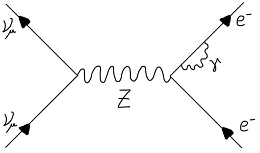
(a) QED radiative correction.

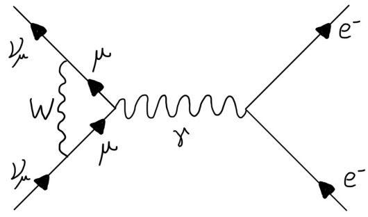
(b) EW radiative correction.

Figure 1: Feynman diagrams representing high order radiative corrections from (a) QED, $e\gamma e$ vertexes and (b) EW, $\mu W\nu_{\mu}$ vertexes.

The expression considering QED and EW radiative corrections for the $\nu_{\mu}e^{-}$ differential cross section takes the form,

$$\frac{d\sigma^{\prime}}{dT} =\frac{2m_{e}G^{2}_{F}}{\pi}\left\{g_{L}^{\prime 2}(T)\left[1+\frac{\alpha}{\pi}f_{-}(z)\right]+g_{R}^{\prime 2}(T)\left(1-\frac{T}{E_{\nu}}\right)^{2}\left[1+\frac{\alpha}{\pi}f_{+}(z)\right]\right.$$

$$\qquad{}\left.-g^{\prime}_{R}(T)g^{\prime}_{L}(T)m_{e}\frac{T}{E_{\nu}^{2}}\left[1+\frac{\alpha}{\pi}f_{+-}(z)\right]\right\},$$ (3)

where the functions $f_{+}(z)$, $f_{-}(z)$, and $f_{+-}(z)$ account for the QED corrections that depend on $z=T/E_{\nu}$. $\alpha$ is the fine-structure constant. The expressions for these functions [33] are given in Appendix A. The values of $f_{+}(z)$, $f_{-}(z)$, and $f_{+-}(z)$ present important variations with the neutrino energy in the range under consideration. For the antineutrino cross section, the $g^{\prime}_{L,R}$ couplings must be interchanged like $g^{\prime}_{L}\leftrightarrow g^{\prime}_{R}$, while the three functions, $f(z)$, are preserved.

The coupling constants now include the EW corrections in the following way:

$$g^{\prime}_{L}(T)=\rho_{\rm NC}\left[\frac{1}{2}-\kappa_{\nu_{l}}(T)\sin^{2}\theta_{W}^{(m_{Z})}\right]$$ (4a)

and

$$g^{\prime}_{R}(T)=-\rho_{\rm NC}\kappa_{\nu_{l}}(T)\sin^{2}\theta_{W}^{(m_{Z})}\,,$$ (4b)

where $\rho_{\rm NC}$ and $\kappa_{\nu_{l}}(T)$ are defined in Eqs. (5) and (2.1) below. $m_{Z}$ is the $Z$ boson mass and $\sin^{2}\theta_{W}^{(m_{Z})}$ is $\sin^{2}\theta_{W}$ calculated at the $m_{Z}$ scale. We follow closely the analytic expressions reported in Ref. [36]. This approach, as we discuss later, allows us to confirm that, as expected, the EW corrections do not have important variations in the energy range of our interest.

$$\rho_{\rm NC}=1+\frac{\hat{\alpha}}{4\pi\hat{s}^{2}}\left\{\frac{3}{4\hat{s}^{2}}\ln c^{2}-\frac{7}{4}+\frac{2\hat{c}_{Z}}{\hat{c}^{2}}+\frac{3}{4}\xi\left[\frac{\ln\left(\frac{c^{2}}{\xi}\right)}{c^{2}-\xi}+\frac{1}{c^{2}}\frac{\ln\xi}{1-\xi}\right]+\frac{3}{4}\frac{m_{t}^{2}}{m_{W}^{2}}\right\},$$ (5)

where $s$ and $c$ stand for sine and cosine of $\theta_{W}$, respectively. Hat over the parameters indicate their values calculated at the $m_{Z}$ scale. $\hat{c}_{Z}=\frac{19}{8}-\frac{7}{2}\hat{s}^{2}+3\hat{s}^{4}\,$, $\xi=\frac{m_{H}^{2}}{m_{Z}^{2}}\,$, and $m_{H,t,W}$ are the masses of the Higgs boson, the top quark, and the $W$ boson respectively. Rho has the numerical value $\rho_{\rm NC}=1.014032$.

$$\kappa_{\nu_{l}}(q^{2}) =1-\frac{\alpha}{2\pi\hat{s}^{2}}\left[\sum_{i}\left(C_{3i}Q_{i}-4\hat{s}^{2}Q_{i}^{2}\right)J_{i}(q^{2})-2J_{l}(q^{2})\right.$$

$$\qquad{}\left.+\ln c\left(\frac{1}{2}-7\hat{c}^{2}\right)+\frac{\hat{c}^{2}}{3}+\frac{1}{2}+\frac{\hat{c}_{\gamma}}{\hat{c}^{2}}\right],$$ (6)

where $C_{3i}$ is twice the third component of weak isospin, $Q_{i}$ represents the electric charge, $\hat{c}_{\gamma}=\frac{19}{8}-\frac{17}{4}\hat{s}^{2}+3\hat{s}^{4}\,$, $q^{2}=-2m_{e}T$ is the squared four-momentum transfer, and

$$J_{i}(q^{2})=\int_{0}^{1}x(1-x)\ln\left(\frac{m_{i}^{2}-q^{2}x(1-x)}{m_{Z}^{2}}\right)dx\,,$$ (7)

where $m_{i}$ is the mass of the $i$th fermion. The sum in Eq. (2.1) includes all the charged fermions, and we consider an additional factor of 3 for quarks (due to the color degree of freedom).

The flavor dependence of the incident neutrino is contained in the $2J_{l}(q^{2})$ term. For a $\nu_{\mu}$ flux, we have $2J_{\mu}(q^{2})$. We can have a first general idea of the different dependence on EW corrections for neutrino and antineutrino electron scattering by considering the simple case of a monoenergetic neutrino beam and focus on the effect of $\kappa_{\nu_{\mu}}$. Now, the cross section is given by an equation similar to Eq. (1), but corrected with the coupling constants,

$$\tilde{g}_{L}\approx\frac{1}{2}-\kappa_{\nu_{\mu}}x$$ (8a)

and

$$\tilde{g}_{R}\approx-\kappa_{\nu_{\mu}}x,$$ (8b)

with $x=\sin^{2}\theta_{W}$ for short.

The differences between the aforementioned differential cross section, considering EW radiative corrections (${d\sigma^{\prime}_{\rm EW}}/{dT}$) and the differential cross section at tree level, Eq. (1), for neutrino and antineutrino, are, respectively,

$$\Delta\sigma_{\nu_{\mu}e}\equiv\frac{d\sigma^{\prime}_{\rm EW}}{dT}-\frac{d\sigma}{dT}\sim\Delta g_{L}+\Delta g_{R}\left(1-2\frac{T}{E_{\nu}}+\frac{T^{2}}{E_{\nu}^{2}}\right)-\Delta g_{R,L}m_{e}\frac{T}{E_{\nu}^{2}}$$ (9a)

and

$$\Delta\sigma_{\bar{\nu}_{\mu}e}\equiv\frac{d\bar{\sigma}^{\prime}_{\rm EW}}{dT}-\frac{d\bar{\sigma}}{dT}\sim\Delta g_{R}+\Delta g_{L}\left(1-2\frac{T}{E_{\nu}}+\frac{T^{2}}{E_{\nu}^{2}}\right)-\Delta g_{R,L}m_{e}\frac{T}{E_{\nu}^{2}}\,,$$ (9b)

where $\Delta g_{L}$, $\Delta g_{R}$, and $\Delta g_{R,L}$ represent the following differences:

$$\Delta g_{L} \equiv\tilde{g}_{L}^{2}-g_{L}^{2}=(\kappa^{2}_{\nu_{\mu}}-1)x^{2}\left[1-\frac{1}{(\kappa_{\nu_{\mu}}+1)x}\right]\,,$$ (10a)

$$\Delta g_{R} \equiv\tilde{g}_{R}^{2}-g_{R}^{2}=(\kappa^{2}_{\nu_{\mu}}-1)x^{2}\,,$$ (10b)

and

$$\Delta g_{R,L} \equiv\tilde{g}_{R}\tilde{g}_{L}-g_{R}g_{L}=(\kappa^{2}_{\nu_{\mu}}-1)x^{2}\left[1-\frac{1/2}{(\kappa_{\nu_{\mu}}+1)x}\right]\,.$$ (10c)

Given $\kappa_{\nu_{\mu}}\approx 1$ and $x\approx 1/4$, we have $(\kappa_{\nu_{\mu}}+1)x\approx 1/2$, which implies

$$\Delta g_{L}\approx-\Delta g_{R}\qquad{\rm and}\qquad\Delta g_{L,R}\approx 0\,,$$ (11)

and, therefore:

$$\Delta\sigma_{\bar{\nu}_{\mu}e}\approx-\Delta\sigma_{\nu_{\mu}e}\approx\Delta g_{R}\left(-2+\frac{T}{E_{\nu}}\right)\frac{T}{E_{\nu}}\,.$$ (12)

This result shows that there is an asymmetric relation between the EW radiative corrections for neutrino and antineutrino scattering. Conversely, if we consider the QED corrections effect, the relative deviation from the tree level is the same for neutrino and antineutrino. These behaviors are illustrated in Fig. 2, where the relative contributions, Eq. (13), of the different groups of corrections are displayed for a hypothetical monoenergetic neutrino beam of 10 GeV.

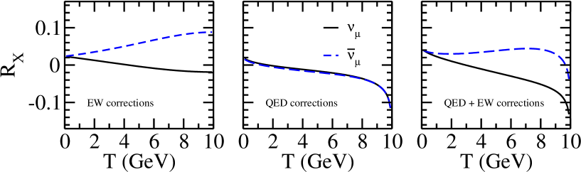
Figure 2: Comparison of the ratio of radiative corrections for neutrino and antineutrino beam modes, for a fixed neutrino energy of 10 GeV. a) Contribution of EW corrections, b) contribution of QED corrections, and c) total contributions.

The deviation from the tree level differential cross section is defined as the ratio,

$$R_{\rm X}\mathrel{\mathop{\mathchar 58\relax}}=\dfrac{\frac{d\sigma^{\prime}_{\rm X}}{dT}-\frac{d\sigma}{dT}}{\frac{d\sigma}{dT}}\,,$$ (13)

where X denotes the inclusion of either EW, QED, or both corrections at the same time. Although the behavior of this ratio was calculated for a fixed neutrino energy, the qualitative behavior persists for the neutrino beam spectrum.

The two different effects (EW + QED corrections, Fig. 2c) change the antineutrino electron scattering cross section, resulting practically always in an increment. This is in opposition to the neutrino case, in which the radiative corrections increase the cross section only in the low energy range, below $\approx 2$ GeV for our study case depicted in Fig. 2, while in the higher energy range the cross section decreases. This behavior will be relevant when studying specific experimental setups, as we evince in Sec. 3.

2.2 Neutrino charge radius

We can now take a careful look at the contribution of $\kappa_{\nu_{l}}(q^{2})$, defined in Eq. (2.1). Depending on the particular process, e.g., for different neutrino flavors, the correction has different values. We can decompose this expression into two parts. The first one, $\kappa_{\nu}(q^{2})$, is a common contribution for all the neutrino flavors:

$$\kappa_{\nu}(q^{2})=1-\frac{\alpha}{2\pi\hat{s}^{2}}\left[\sum_{i}\left(C_{3i}Q_{i}-4\hat{s}^{2}Q_{i}^{2}\right)J_{i}(q^{2})+\ln c\left(\frac{1}{2}-7\hat{c}^{2}\right)+\frac{\hat{c}^{2}}{3}+\frac{\hat{c}_{\gamma}}{\hat{c}^{2}}\right].$$ (14)

In the energy region of interest for this work, this contribution takes the value $\kappa_{\nu}(q^{2})=1.017$.

The second contribution is flavor dependent,

$$-\frac{\alpha}{2\pi\hat{s}^{2}}\left[-2J_{l}(q^{2})+\frac{1}{2}\right],$$ (15)

and its numerical value in this region is $-0.025$.

This is responsible for the difference of around $3\%$ between $\kappa_{\nu_{\mu}}$, Eq. (2.1), and $\kappa_{\nu}$, Eq. (14), shown in Fig. 3. When $Q\equiv\sqrt{-q^{2}}$ tends to zero, the values of $\kappa$, i.e., the value of the flavor dependent part, Eq. (15), remains constant. This encompasses the energy range of our interest in this work, limited by the shaded vertical band in the figure.

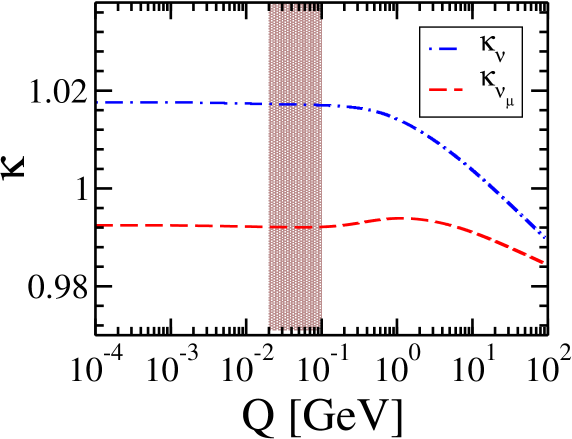
Figure 3: $\kappa_{\nu}$ and $\kappa_{\nu_{\mu}}$ as functions of $Q$. The dot-dashed blue line represents $\kappa_{\nu}$, Eq. (14), and the dashed red line represents $\kappa_{\nu_{\mu}}$, Eq. (2.1). The shaded area represents the electron recoil energy (T) where we investigate the effect of radiative corrections and the experimental sensitivity to the neutrino charge radius.

We turn our attention to $-2J_{l}(q^{2})+\frac{1}{2}$, from Eq. (15), which when evaluated in $q=0$ becomes

$$-2J_{l}(0)+\frac{1}{2}=\frac{1}{6}\left[3-2\ln\left(\frac{m^{2}_{l}}{m^{2}_{Z}}\right)\right].$$ (16)

This quantity  is usually associated with the neutrino charge radius (NCR),

$$\left\langle r^{2}_{\nu_{l}}\right\rangle=\frac{G_{F}}{4\sqrt{2}\pi^{2}}\left[3-2\ln\left(\frac{m^{2}_{l}}{m^{2}_{W}}\right)\right],$$ (17)

for which the reported value for the $\mu$ flavor is $\left\langle r^{2}_{\nu_{\mu}}\right\rangle=2.4\times 10^{-33}$ cm² [11].

We can also separate the couplings $g^{\prime}_{L}(T)$ and $g^{\prime}_{R}(T)$ into two parts, one independent of the incoming neutrino flavor and the other in terms of the NCR as [11],

$$g_{L,R}^{\prime(\nu_{\mu},e)}(T)\sim g_{L,R}^{\prime(\nu,e)}(T)+\left[\frac{2}{3}m_{W}^{2}\left\langle r^{2}_{\nu_{\mu}}\right\rangle\right]\sin^{2}\theta_{W}^{(m_{Z})},$$ (18)

where the numerical value of $\left[\frac{2}{3}m_{W}^{2}\left\langle r^{2}_{\nu_{\mu}}\right\rangle\right]\sin^{2}\theta_{W}^{(m_{Z})}$ is $\approx 0.0058$.

The numerical values of $\kappa$ and the couplings are reported in Table 1. The first row shows the flavor independent values, i.e., without the term containing the NCR. The second row shows the values including the NCR term.

Table 1: Numerical value of $\kappa$ (evaluated at $q^{2}=0$) and of the couplings $g^{\prime}_{L}(T)$ and $g^{\prime}_{R}(T)$, depending on the inclusion of the neutrino charge radius term.

NCR	$\kappa$	$g^{\prime}_{L}$	$g^{\prime}_{R}$
no	1.0176	0.2684	-0.2386
yes	0.9925	0.2743	-0.2327

3 The DUNE case

The Deep Underground Neutrino Experiment (DUNE) [42] is part of one of the most ambitious neutrino experimental programs in the world, consisting of two detectors separated by a baseline of approximately 1300 km. There will be a 40 kt far detector (FD) [43] in South Dakota and a near detector (ND) [27] in Illinois at the Fermi National Accelerator Laboratory. The ND measures the flux spectrum with no oscillation for all the neutrino types coming from the beam. To achieve DUNE measurement goals of precision, the ND must provide constraints on the systematic uncertainties such as the absolute and relative flux, nuclear effects, and neutrino type determination. It is expected to achieve very precise measurements of neutrino interactions. There are a few ND design options, but in this work, we assume the LArTPC design, which uses the same technology as the FD.

In order to minimize the systematic uncertainties in the flux, cross section, and detector effects in the energy spectrum, a movable near detector concept was proposed, called DUNE-PRISM [44, 28]. With PRISM, it is possible to collect data at several off axis angles up to a maximum of $3.6^{\circ}$, exposing the ND to different fluxes and spectra.

To explore DUNE-PRISM sensitivity to the NCR, we calculate the expected number of events generated from $\nu_{\mu}e^{-}$ scattering for on axis and different off axis beam angles. Then we analyze what can be the best angular window and energy range to measure differences in the number of events related to the radiative corrections, especially the NCR effect.

For this purpose, we consider the predicted neutrino energy spectra for the different incident beam angles. We consider the fluxes reported in Ref. [45]. These fluxes are shown in Fig. 4 with the simulated data represented by different symbols for each different beam direction and with the data interpolation lines.

(a) $\nu_{\mu}$ beam mode

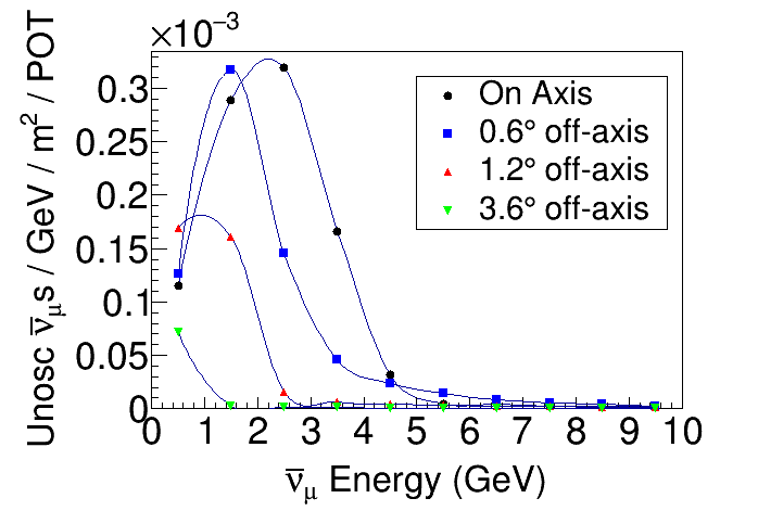
(b) $\bar{\nu}_{\mu}$ beam mode

Figure 4: Fluxes at several off axis locations [45]. Neutrino mode (a), on the left side, and antineutrino mode (b), on the right side. The symbols represent the simulated data, and the lines show their interpolation.

The number of targets in the detector corresponds to the number of electrons in the total mass of liquid argon, considered to be 75 t [28]. The experiment is expected to run for 3.5 years in the neutrino mode and the same period in the antineutrino mode. Given these assumptions, we compute the expected number of events without or with radiative corrections, in which case, we can separate and distinguish the NCR contribution to the corrections.

For each PRISM axis configuration, in terms of angular location, we must compute the average cross section. That is given by the integral from the threshold electron recoil energy, $T_{min}$, up to a maximum kinetically allowed value, $T_{max}\approx E_{\nu}^{max}$, so

$$\sigma=\int_{T_{min}}^{T_{max}}f(T)dT,$$ (19)

where $f(T)$ is the integral of the differential cross section, $\frac{d\sigma}{dT}\left(T,E_{\nu}\right)$, times the corresponding neutrino flux, $\lambda(E_{\nu})$,

$$f(T)=\int_{E_{\nu}^{min}(T)}^{E_{\nu}^{max}}\frac{d\sigma}{dT}\left(T,E_{\nu}\right)\lambda(E_{\nu})dE_{\nu}\,,$$ (20)

where $E_{\nu}^{min}(T)$ is the minimum neutrino energy considered and given by the detector’s electron energy threshold.

Once we compute the cross section, Eq. (19), it is necessary to take into account the detector exposure to obtain the number of events,

$$N=\sigma\times\mathscr{C}\,,$$ (21)

where $\mathscr{C}$ is the exposure. It takes into account the number of target electrons in the detector, the number of protons on target per year of $1.1\times 10^{21}$ POT/year [45], and 3.5 years in the neutrino beam mode plus 3.5 years in the antineutrino beam mode.

As discussed in Sec. 2.1, it is expected that, when radiative corrections are considered, the antineutrino electron scattering cross section have an increase with respect to the tree level calculation. This results in an increase in the expected number of events as well. It is not the case for the neutrino mode in which, as we discuss in the next section, a decrease in the expected number of events is predicted for electron recoil energies above approximately $0.7$ GeV.

3.1 Results and discussion

Table 2: The total number of events from $\bar{\nu}_{\mu}e$ scattering for an energy range of 0.2 to 10 GeV, considering the tree level and radiative corrections with and without neutrino charge radius (NCR). The first column shows the DUNE-PRISM axis location. $\sigma_{stat}$ is the statistical error and $\Delta$ is the difference between the number of events calculated at tree level and with radiative corrections. See text for details.

	Number of $\bar{\nu}_{\mu}$ Events
			Without NCR		With NCR
Axis location	Tree level	$\sigma_{stat}$	EW+QED	$\Delta$	EW+QED	$\Delta$
0.0$\degree$	18775	137	19931	1156	19447	672
0.6$\degree$	11969	109	12715	746	12402	433
1.2$\degree$	3993	63	4251	258	4141	148
1.8$\degree$	1181	34	1260	79	1226	45
2.4$\degree$	645	25	689	44	670	25
3.0$\degree$	437	21	467	30	454	17
3.6$\degree$	315	18	336	21	327	12

We show our results considering two different electron recoil energy thresholds. The first is 0.2 GeV, and the second is 0.7 GeV. The second threshold is used to maximize the difference in the number of events between the tree level calculation and the radiative corrections for the neutrino beam mode. For on axis neutrino beam, the effect of radiative corrections is opposite below and above the threshold of $\sim 0.7$ GeV. When the differential cross section is integrated, this ends up diminishing the total event number difference. This is why considering this crossing point as the threshold helps to enlarge the difference that we need to detect in the case of neutrino scattering. Considering this crossing point as the threshold helps to enlarge the difference between the tree level and the one loop level predictions. For antineutrinos, radiative corrections increase the expected number of events, independent of the energy range observed.

Table 3: The total number of events from $\nu_{\mu}e$ scattering for an energy range of 0.2 to 10 GeV, considering the tree level and radiative corrections with and without neutrino charge radius. The first column shows the DUNE-PRISM axis location. $\sigma_{stat}$ is the statistical error and $\Delta$ is the difference between the number of events calculated at tree level and with radiative corrections. See text for details.

	Number of $\nu_{\mu}$ Events
			Without NCR		With NCR
Axis location	Tree level	$\sigma_{stat}$	EW+QED	$\Delta$	EW+QED	$\Delta$
0.0$\degree$	27134	165	25859	-1275	26567	-567
0.6$\degree$	18099	135	17243	-856	17712	-387
1.2$\degree$	5884	77	5589	-295	5749	-135
1.8$\degree$	2600	51	2466	-134	2538	-62
2.4$\degree$	1397	37	1324	-73	1364	-33
3.0$\degree$	711	27	674	-37	694	-17
3.6$\degree$	440	21	418	-22	430	-10

In Table 2 and Table 3, we summarize the results for antineutrino and neutrino events, respectively. The energy range considered in the calculation is 0.2 GeV to 10.0 GeV. We give the results for the DUNE-PRISM axis location from 0$\degree$ to 3.6$\degree$ in intervals of 0.6$\degree$ and show the NCR’s contribution in the radiative corrections. Considering the NCR, the difference in the number of events, $|\Delta|$, in comparison with the tree level calculation, is larger for antineutrino than for neutrino. More importantly, we see in these tables that the difference in the number of events is bigger than the statistical error for off axis angles equal to or smaller than $1.8\degree$. In particular, for the on axis case, the statistical error is remarkably small in comparison to the difference in the number of events. Therefore, if the systematic uncertainties can be under control, a determination of the NCR may be possible.

Table 4: The total number of events for $\bar{\nu}_{\mu}$ and $\nu_{\mu}$ beam modes, on axis, within the energy range from 0.7 to 10 GeV, considering the tree level and radiative corrections with and without neutrino charge radius. $\sigma_{stat}$ is the statistical error and $\Delta$ is the difference between the number of events calculated at tree level and with radiative corrections. See text for details.

	Number of Events
			Without NCR		With NCR
	Tree level	$\sigma_{stat}$	EW+QED	$\Delta$	EW+QED	$\Delta$
$\bar{\nu}_{\mu}$	12935	114	13850	915	13420	485
$\nu_{\mu}$	19947	141	18715	-1232	19318	-629

The results for the neutrino beam mode are shown in Table 3, where we see that $|\Delta|$ (with NCR) is smaller than for the antineutrino mode, Table 2. Notice that the neutrino mode is expected to generate a larger number of events than the antineutrino one. However, $|\Delta|$ (with NCR) is smaller for neutrinos due to the radiative corrections sign’s change. See Fig. 2.

The other case of interest to consider is that of a threshold of $0.7$ GeV, which corresponds to the already mentioned crossing point for the neutrino mode. Starting from this energy, the radiative corrections for the $\nu_{\mu}e^{-}$ are always negative, making the effect for this case more visible than for the $0.2$ GeV threshold. See Table 4. Since the neutrino production is in general higher in this type of beams, we can expect this result to be a general characteristic of this type of experiments. Moreover, this shows the importance of setting up the energy threshold based on the kind of physics measurement to be conducted, instead of simply lowering the threshold based only in detector characteristics.

In Fig. 5, we show the expected number of events per bin of electron recoil energy for two different incident antineutrino beam angles. The 2 GeV range for each bin is chosen conservatively, as the expected energy resolution for a DUNE ND-like detector is of the order of 10% for energies above 0.2 GeV [46]. As already stated, there is better statistics when we consider the on axis position, which translates in a smaller error. For antineutrino fluxes at other angles, the statistics is worse, as is shown in the right panel of the same Fig. 5, for an angle of $0.6\degree$. For larger angles, the statistics are even lower. We can also notice from this figure that the first energy bin shows the most relevant difference between the number of events for tree level and radiative correction expected measurements. Finally, it is also evident from this figure that in the antineutrino mode, a low energy threshold is very useful to have this kind of signature.

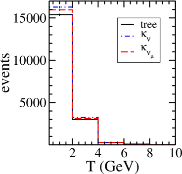
(a) On-axis

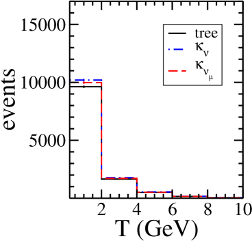
(b) 0.6$\degree$ off-axis

Figure 5: Comparison among the number of $\bar{\nu}_{\mu}$ event expectations at tree-level (solid black line) and considering radiative corrections, with and without neutrino charge radius (dashed red and dot-dashed blue line, respectively). We show two DUNE-PRISM spectra: (a) On axis on the left and (b) 0.6$\degree$ on the right side.

In Fig. 6, we show the results for the case of muon neutrinos. We notice that the radiative corrections have an opposite contribution to the expected number of events as already forecast. It is also important to point out that the overall radiative correction contribution is smaller for the neutrino mode than for the antineutrino one. As already discussed, the reason is the cancellation that occurs when considering two energy windows: the radiative corrections in the neutrino mode change sign in the first bin of energy; i.e., they have a positive contribution for energies below approximately 0.7 GeV and a negative contribution for energies above that limit.

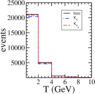
(a) On-axis

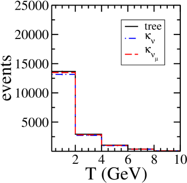
(b) 0.6$\degree$ off-axis

Figure 6: Comparison among the number of $\nu_{\mu}$ event expectations at tree-level (solid black line) and considering radiative corrections, with and without neutrino charge radius (dashed red and dot-dashed blue line, respectively). We show two DUNE-PRISM spectra: (a) On axis on the left and (b) 0.6$\degree$ on the right side.

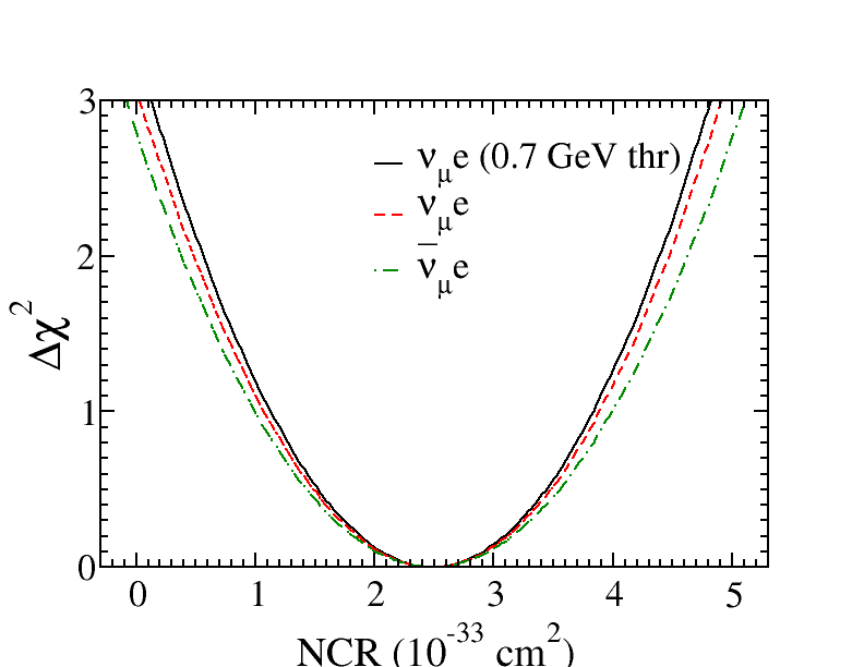
(a) 3% systematics

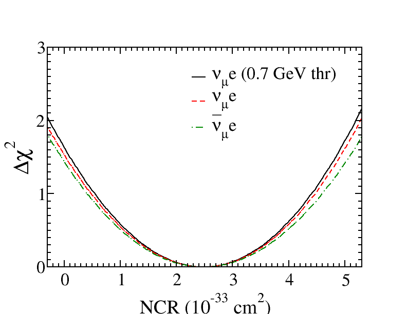
(b) 5% systematics

Figure 7: Expected sensitivity to the electroweak radiative corrections for a 3% systematic error (a) Left; and 5% systematic error (b) Right. We show $\Delta\chi^{2}=\chi^{2}-\chi^{2}_{\rm min}$ as a function of the neutrino charge radius (NRC). Red dashed and green dot-dashed lines correspond to a 0.2 GeV threshold in the $\nu$ and $\bar{\nu}$ scattering, while the black line corresponds to the 0.7 GeV $\nu$ scattering threshold. Neutrino data with 0.7 GeV threshold and 3% systematic error can reach a better than 90% confidence level sensitivity to the NCR within our assumptions. See text for details.

Finally, to estimate the sensitivity to the radiative corrections, we conduct a $\chi^{2}$ analysis considering the expected number of events at a DUNE-PRISM like experiment with its statistical and systematic uncertainties. For this purpose, we assume that the experiment will measure the SM prediction including radiative corrections. We define the $\chi^{2}$ function as

$$\chi^{2}=\sum_{i=1}^{5}\dfrac{(N^{exp}_{i}-N^{theo}_{i})^{2}}{(\sigma^{2}_{stat}+\sigma^{2}_{syst})_{i}}\,,$$ (22)

where $i$ is the energy bin, $N^{exp}$ refers to the expected number of events that the SM predicts, considering electroweak and QED radiative corrections, and $N^{theo}$ refers to the theoretically calculated number of events for different values of $\kappa$ (Eq. 2.1). The statistical and systematic uncertainties are given by $\sigma_{stat}$ and $\sigma_{syst}$, respectively. We assume the statistical uncertainty to be the square root of the number of events, $\sigma_{stat}=\sqrt{N^{exp}}$, and the systematic to be 3% or 5% error. We also define $\Delta\chi^{2}=\chi^{2}-\chi^{2}_{\rm min}$, where $\chi^{2}_{\rm min}$ is the minimum value of $\chi^{2}$.

The results with different systematic uncertainties are depicted in Fig. 7, where we see that it may be possible to distinguish the prediction $\kappa_{\nu_{\mu}}=0.9925$, for radiative corrections with NCR, from the case without NCR, $\kappa_{\nu}=1.0176$. A $3\%$ systematic error would be sensitive, at $1\sigma$ precision, to a NCR in the range from $1.0$ to $4.0$ $\times 10^{-33}$ cm² for the antineutrino channel, and from $1.1$ to $3.9$ $\times 10^{-33}$ cm² for the neutrino channel, and, finally, from $1.1$ to $3.8$ $\times 10^{-33}$ cm² for the neutrino channel with the energy threshold of $0.7$ GeV. Even in the case of a $5$% systematic error, it is still possible to have a precision higher than $1\sigma$. In contrast, the current constraint reported in the PDG for $\nu_{\mu}e$ scattering is in the range from $-5.3$ to $6.8$ $\times 10^{-33}$ cm² [39], which is still consistent with no NCR.

Besides this analysis, we have also performed a different computation shown in Fig. (8). For this computation we consider the $\Delta\chi^{2}$ with a theoretical prediction where no radiative corrections are taken into account at all, that is, the tree level. We show in this figure that, depending on the systematic uncertainties, the radiative corrections can be distinguished from the tree level or not. For the neutrino case we consider, as discussed above, an appropriate energy range from $0.7$ to $10$ GeV to improve the sensitivity, while for the antineutrino case we consider an energy range starting from $0.2$ GeV. We have considered five energy bins in both cases. The results are shown for two different incoming neutrino angles. We can notice that the neutrino case is very promising in its sensitivity to radiative corrections even for relatively large systematic errors and for different incoming neutrino fluxes thanks to the combination of high statistics and a suitable energy window. For the antineutrino case it is also possible to have a discrimination, but the systematic errors should be under control, approximately below 4%.

We could have even better discrimination of the radiative corrections if we combine both neutrino and antineutrino signals. We notice that radiative corrections have opposite effects on neutrino and antineutrino electron scattering, resulting in a cross section decrease for muon neutrino scattering off electrons but an increase for antineutrino interactions. This suggests that it might be possible to define the difference between these two signals as an observable to evaluate the neutrino charge radius better. A detailed analysis in this direction would require a good knowledge of the correlation between both signals.

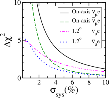
Figure 8: Expected sensitivity, in terms of $\Delta\chi^{2}=\chi^{2}-\chi^{2}_{\rm min}$, to differentiate between the tree level and the radiative corrections case, depending on the systematic error. We show the results for two different locations of the detector (on axis and $1.2^{\circ}$) and for neutrino (solid and dash-dotted) and antineutrino (dashed and dotted) electron scattering. For the neutrino electron case, we have chosen an energy threshold of $0.7$ GeV to improve the sensitivity.

4 Conclusions

The precise determination of the radiative corrections at low energies is of great importance to test the SM. An accurate determination of the weak mixing angle in the low energy region of accelerator-based neutrino experiments is in order, as well as an experimental probe that the neutrino charge radius (NCR), as an effective observable, is present in this process. Moreover, accurate tests of physics beyond the SM will find a limitation if these observables are not well determined.

We have studied the sensitivity of future near detectors, like in long-baseline neutrino experimental facilities, to radiative corrections in neutrino-electron scattering, considering the case of DUNE-PRISM as an illustrative example. We focus on the NCR as an effective observable that is characteristic of this process. Since the NCR main effect is a shift in the weak mixing angle, we have investigated the detector sensitivity to radiative corrections, separating the NCR effect. Taking as a guidance, the DUNE-PRISM configuration that would allow several beam angle setups, we have analyzed different neutrino energy spectra. We find that on axis neutrino spectrum will allow a better determination of the radiative corrections and possibly the NCR due to its higher statistics. We have illustrated that with a systematic error of the order of $3$% there are good expectations to measure the NCR with an error of the order of $1.5\times 10^{-33}$ cm².

Our analysis shows that for the case of a $\nu_{\mu}$ beam, a correct selection of the energy window could allow us to determine the existence of the NCR if the systematic uncertainties are under control, thanks to the high statistics expected in this beam mode. On the other hand, for the $\bar{\nu}_{\mu}$ mode, we have pointed out that the best chance to measure this effective observable is for small electron recoil energy values. Therefore, in this case, the lower the threshold, the better for such a measurement.

Appendix A QED Functions

In this appendix, we show the explicit form of the functions $f_{-}(z)$, $f_{+}(z)$, and $f_{+-}(z)$ that are introduced in Eq. (2.1). We consider the expressions given in Ref. [33] (numerical expressions can be found in Ref. [34]) and that for the case of $f_{-}(z)$ is

$$f_{-}(z) =\left[\frac{E}{l}\ln\left(\frac{E+l}{m_{e}}\right)-1\right]\left[2\ln\left(1-z-\frac{m_{e}}{E+l}\right)-\ln\left(1-z\right)-\frac{1}{2}\ln z-\frac{5}{12}\right]$$

$$\qquad{}+\frac{1}{2}\left[L(z)-L(\beta)\right]-\frac{1}{2}\ln^{2}\left(1-z\right)-\left(\frac{11}{12}+\frac{z}{2}\right)\ln\left(1-z\right)$$

$$\qquad{}+z\left[\ln z+\frac{1}{2}\ln\left(\frac{2E_{\nu}}{m_{e}}\right)\right]-\left(\frac{31}{18}+\frac{1}{12}\ln z\right)\beta-\frac{11}{12}z+\frac{z^{2}}{24}\,,$$ (23)

where $l=\sqrt{E^{2}-m^{2}_{e}}\,$ is the three-momentum of the electron, $E=T+m_{e}$, $\beta=l/E$, and $L(x)$ is in Spence’s function space corresponding to the following dilogarithm:

$$L(x)=-Li_{2}(x)=\int_{0}^{x}\frac{\ln\mathinner{\!\left\lvert 1-t\right\rvert}}{t}dt\,.$$ (24)

The $f_{+}(z)$ function is given by

$$\left(1-z\right)^{2}f_{+}(z) =\left[\frac{E}{l}\ln\left(\frac{E+l}{m_{e}}\right)-1\right]\left\{\left(1-z\right)^{2}\left[2\ln\left(1-z-\frac{m_{e}}{E+l}\right)\right.\right.$$

$$\qquad{}\left.\left.-\ln\left(1-z\right)-\frac{1}{2}\ln z-\frac{2}{3}\right]-\frac{z^{2}\ln z+1-z}{2}\right\}$$

$$\qquad{}-\frac{\left(1-z\right)^{2}}{2}\left\{\ln^{2}\left(1-z\right)+\beta\left[L(1-z)-\ln z\ln\left(1-z\right)\right]\right\}$$

$$\qquad{}+\ln\left(1-z\right)\left[\frac{z^{2}}{2}\ln z+\frac{1-z}{3}\left(2z-\frac{1}{2}\right)\right]-\frac{z^{2}}{2}L\left(1-z\right)$$

$$\qquad{}-\frac{z\left(1-2z\right)}{3}\ln z-\frac{z\left(1-z\right)}{6}$$

$$\qquad{}-\frac{\beta}{12}\left[\ln z+\left(1-z\right)\left(\frac{115-109z}{6}\right)\right]\,,$$ (25)

and the $f_{+-}(z)$ function is

$$f_{+-}(z) =\left[\frac{E}{l}\ln\left(\frac{E+l}{m_{e}}\right)-1\right]2\ln\left(1-z-\frac{m_{e}}{E+l}\right)\,.$$ (26)

References

- [1] F. J. Hasert et al. [Gargamelle Neutrino], Phys. Lett. 46B (1973), 138-140 doi:10.1016/0370-2693(73)90499-1
- [2] S. L. Glashow, Nucl. Phys. 22, 579-588 (1961) doi:10.1016/0029-5582(61)90469-2
- [3] S. Weinberg, Phys. Rev. Lett. 19, 1264-1266 (1967) doi:10.1103/PhysRevLett.19.1264
- [4] S. L. Glashow and S. Weinberg, Phys. Rev. D 15, 1958 (1977) doi:10.1103/PhysRevD.15.1958
- [5] A. Salam, Conf. Proc. C 680519, 367-377 (1968) doi:10.1142/9789812795915_0034
- [6] P. Vilain et al. [CHARM-II], Phys. Lett. B 335, 246-252 (1994) doi:10.1016/0370-2693(94)91421-4
- [7] C. Anderson et al. [ArgoNeuT], Phys. Rev. Lett. 108, 161802 (2012) doi:10.1103/PhysRevLett.108.161802 [arXiv:1111.0103 [hep-ex]].
- [8] Y. Farzan and M. Tortola, Front. in Phys. 6, 10 (2018) doi:10.3389/fphy.2018.00010 [arXiv:1710.09360 [hep-ph]].
- [9] T. Ohlsson, Rept. Prog. Phys. 76, 044201 (2013) doi:10.1088/0034-4885/76/4/044201 [arXiv:1209.2710 [hep-ph]].
- [10] O. G. Miranda and H. Nunokawa, New J. Phys. 17, no.9, 095002 (2015) doi:10.1088/1367-2630/17/9/095002 [arXiv:1505.06254 [hep-ph]].
- [11] C. Giunti and A. Studenikin, Rev. Mod. Phys. 87 (2015), 531 doi:10.1103/RevModPhys.87.531 [arXiv:1403.6344 [hep-ph]].
- [12] B. C. Canas, O. G. Miranda, A. Parada, M. Tortola and J. W. F. Valle, Phys. Lett. B 753, 191-198 (2016) doi:10.1016/j.physletb.2015.12.011 [arXiv:1510.01684 [hep-ph]].
- [13] Z. Daraktchieva et al. [MUNU], Phys. Lett. B 615, 153-159 (2005) doi:10.1016/j.physletb.2005.04.030 [arXiv:hep-ex/0502037 [hep-ex]].
- [14] K. S. Kumar, S. Mantry, W. J. Marciano and P. A. Souder, Ann. Rev. Nucl. Part. Sci. 63, 237-267 (2013) doi:10.1146/annurev-nucl-102212-170556 [arXiv:1302.6263 [hep-ex]].
- [15] W. J. Marciano and J. L. Rosner, Phys. Rev. Lett. 65, 2963-2966 (1990) [erratum: Phys. Rev. Lett. 68, 898 (1992)] doi:10.1103/PhysRevLett.65.2963
- [16] O. Tomalak, P. Machado, V. Pandey and R. Plestid, J. High Energy Phys. 02 (2021) 097 doi:10.1007/JHEP02(2021)097 [arXiv:2011.05960 [hep-ph]].
- [17] M. Cadeddu and F. Dordei, Phys. Rev. D 99, no.3, 033010 (2019) doi:10.1103/PhysRevD.99.033010 [arXiv:1808.10202 [hep-ph]].
- [18] B. C. Cañas, E. A. Garcés, O. G. Miranda and A. Parada, Phys. Lett. B 784, 159-162 (2018) doi:10.1016/j.physletb.2018.07.049 [arXiv:1806.01310 [hep-ph]].
- [19] M. Deniz et al. [TEXONO], Phys. Rev. D 81, 072001 (2010) doi:10.1103/PhysRevD.81.072001 [arXiv:0911.1597 [hep-ex]].
- [20] A. de Gouvea, P. A. N. Machado, Y. F. Perez-Gonzalez and Z. Tabrizi, Phys. Rev. Lett. 125, no.5, 051803 (2020) doi:10.1103/PhysRevLett.125.051803 [arXiv:1912.06658 [hep-ph]].
- [21] C. M. Marshall, K. S. McFarland and C. Wilkinson, Phys. Rev. D 101, no.3, 032002 (2020) doi:10.1103/PhysRevD.101.032002 [arXiv:1910.10996 [hep-ex]].
- [22] S. Sarantakos, A. Sirlin and W. J. Marciano, Nucl. Phys. B 217, 84-116 (1983) doi:10.1016/0550-3213(83)90079-2
- [23] J. L. Lucio, A. Rosado and A. Zepeda, Phys. Rev. D 29, 1539 (1984) doi:10.1103/PhysRevD.29.1539
- [24] L. G. Cabral-Rosetti, J. Bernabeu, J. Vidal and A. Zepeda, Eur. Phys. J. C 12, 633-642 (2000) doi:10.1007/s100520000304 [arXiv:hep-ph/9907249 [hep-ph]].
- [25] K. Fujikawa and R. Shrock, Phys. Rev. D 69, 013007 (2004) doi:10.1103/PhysRevD.69.013007 [arXiv:hep-ph/0309329 [hep-ph]].
- [26] J. Papavassiliou, J. Bernabeu, D. Binosi and J. Vidal, Eur. Phys. J. C 33, S865-S867 (2004) doi:10.1140/epjcd/s2003-03-920-7 [arXiv:hep-ph/0310028 [hep-ph]].
- [27] D. Hongyue [DUNE], PoS NuFact2017, 058 (2018) doi:10.22323/1.295.0058
- [28] V. De Romeri, K. J. Kelly and P. A. N. Machado, Phys. Rev. D 100, no.9, 095010 (2019) doi:10.1103/PhysRevD.100.095010 [arXiv:1903.10505 [hep-ph]].
- [29] D. Brailsford [SBND], J. Phys. Conf. Ser. 888, no.1, 012186 (2017) doi:10.1088/1742-6596/888/1/012186
- [30] N. McConkey [SBND], PoS NuFact2017, 067 (2018) doi:10.22323/1.295.0067
- [31] M. Antonello et al. [MicroBooNE, LAr1-ND and ICARUS-WA104], [arXiv:1503.01520 [physics.ins-det]].
- [32] C. Farnese [ICARUS], Universe 5, no.2, 49 (2019) doi:10.3390/universe5020049
- [33] J. N. Bahcall, M. Kamionkowski and A. Sirlin, Phys. Rev. D 51, 6146-6158 (1995) doi:10.1103/PhysRevD.51.6146 [arXiv:astro-ph/9502003 [astro-ph]].
- [34] M. Passera, Phys. Rev. D 64, 113002 (2001) doi:10.1103/PhysRevD.64.113002 [arXiv:hep-ph/0011190 [hep-ph]].
- [35] M. Passera, J. Phys. G 29, 141-152 (2003) doi:10.1088/0954-3899/29/1/315 [arXiv:hep-ph/0102212 [hep-ph]].
- [36] A. Sirlin and A. Ferroglia, Rev. Mod. Phys. 85, no.1, 263-297 (2013) doi:10.1103/RevModPhys.85.263 [arXiv:1210.5296 [hep-ph]].
- [37] A. Ferroglia, G. Ossola and A. Sirlin, Eur. Phys. J. C 34, 165-171 (2004) doi:10.1140/epjc/s2004-01604-1 [arXiv:hep-ph/0307200 [hep-ph]].
- [38] J. Erler and R. Ferro-Hernández, JHEP 03, 196 (2018) doi:10.1007/JHEP03(2018)196 [arXiv:1712.09146 [hep-ph]].
- [39] P.A. Zyla et al. [Particle Data Group], PTEP 2020, no.8, 083C01 (2020) doi:10.1093/ptep/ptaa104
- [40] O. Tomalak and R. J. Hill, Phys. Rev. D 101, no.3, 033006 (2020) doi:10.1103/PhysRevD.101.033006 [arXiv:1907.03379 [hep-ph]].
- [41] I. Bischer and W. Rodejohann, Phys. Rev. D 99, no.3, 036006 (2019) doi:10.1103/PhysRevD.99.036006 [arXiv:1810.02220 [hep-ph]].
- [42] B. Abi et al. [DUNE], JINST 15, no.08, T08008 (2020) doi:10.1088/1748-0221/15/08/T08008 [arXiv:2002.02967 [physics.ins-det]].
- [43] B. Abi et al. [DUNE], [arXiv:2002.03005 [hep-ex]].
- [44] C. Vilela, ”DUNE PRISM”, Talk at Physics Opportunities in the Near DUNE Detector Hall (PONDD), 3-7 December, 2019, Batavia, IL, USA, DOI: 10.5281/zenodo.2642370, URL: https://doi.org/10.5281/zenodo.2642370 .
- [45] L. Fields, https://home.fnal.gov/~ljf26/DUNEFluxes/
- [46] A. Abed Abud et al. [DUNE], “Deep Underground Neutrino Experiment (DUNE) Near Detector Conceptual Design Report,” [arXiv:2103.13910 [physics.ins-det]].