Targeted Branching for the Maximum Independent Set Problem

Abstract

Finding a maximum independent set is a fundamental NP-hard problem that is used in many real-world applications. Given an unweighted graph, this problem asks for a maximum cardinality set of pairwise non-adjacent vertices. In recent years, some of the most successful algorithms for solving this problem are based on the branch-and-bound or branch-and-reduce paradigms. In particular, branch-and-reduce algorithms, which combine branch-and-bound with reduction rules, have been able to achieve substantial results, solving many previously infeasible real-world instances. These results were to a large part achieved by developing new, more practical reduction rules. However, other components that have been shown to have a significant impact on the performance of these algorithms have not received as much attention. One of these is the branching strategy, which determines what vertex is included or excluded in a potential solution. Even now, the most commonly used strategy selects vertices solely based on their degree and does not take into account other factors that contribute to the performance of the algorithm.

In this work, we develop and evaluate several novel branching strategies for both branch-and-bound and branch-and-reduce algorithms. Our strategies are based on one of two approaches which are motivated by existing research. They either (1) aim to decompose the graph into two or more connected components which can then be solved independently, or (2) try to remove vertices that hinder the application of a reduction rule which can lead to smaller graphs. Our experimental evaluation on a large set of real-world instances indicates that our strategies are able to improve the performance of the state-of-the-art branch-and-reduce algorithm by Akiba and Iwata. To be more specific, our reduction-based packing branching rule is able to outperform the default branching strategy of selecting a vertex of highest degree on $65\%$ of all instances tested. Furthermore, our decomposition-based strategy based on edge cuts is able to achieve a speedup of $2.29$ on sparse networks ($1.22$ on all instances).

1 Introduction

An independent set of a graph $G=(V,E)$ is a set of vertices $I\subseteq V$ of $G$ such that no two vertices in this set are adjacent. The problem of finding such an independent set of maximum cardinality, the maximum independent set problem, is a fundamental NP-hard problem [15]. Its applications cover a wide variety of fields including computer graphics [33], network analysis [31], route planning [24] and computational biology [4, 8]. In computer graphics for instance, large independent sets can be used to optimize the traversal of mesh edges in a triangle mesh. Further applications stem from its complementary problems minimum vertex cover and maximum clique.

One of the best known techniques for finding maximum independent sets, both in theory [39, 7] and practice [1], are data reduction algorithms. These algorithms apply a set of reduction rules to decrease the size of an instance while maintaining the ability to compute an optimal solution afterwards. A recently successful type of data reduction algorithm is so-called branch-and-reduce algorithms [1, 19], which exhaustively apply a set of reduction rules to compute an irreducible graph. If no further rule can be applied, the algorithm branches into (at least) two smaller subproblems, which are then solved recursively. To make them more efficient in practice, these algorithms also make use of problem-specific upper and lower bounds to quickly prune the search space.

Due to the practical impact of data reduction, most of the research aimed at improving the performance of branch-and-reduce algorithms so far has been focused on either proposing more practically efficient special cases of already existing rules [6, 9], or maintaining dependencies between reduction rules to reduce unnecessary checks [2, 20]. However, improving other aspects of branch-and-reduce has been shown to benefit its performance [30]. The branching strategy in particular has been shown to have a significant impact on the running time [1]. Up to now, the most frequently used branching strategy employed in many state-of-the-art solvers selects branching vertices solely based on their degree. Other factors, such as the actual reduction rules used during the algorithm are rarely taken into account. However, recently there have been some attempts to incorporate such branching strategies for other problems such as finding a maximum $k$-plex [14].

1.1 Contribution

In this paper, we propose and examine several novel strategies for selecting branching vertices. These strategies follow two main approaches that are motivated by existing research: (1) Branching on vertices that decompose the graph into several connected components that can be solved independently. Solving components individually has been shown to significantly improve the performance of branch-and-reduce in practice, especially when the size of the largest component is small [2]. (2) Branching on vertices whose removal leads to reduction rules becoming applicable again. In turn, this leads to a smaller reduced graph and thus improved performance. For each approach we present several concrete strategies that vary in their complexity. Finally, we evaluate their performance by comparing them to the aforementioned default strategy used in the state-of-the-art solver by Akiba and Iwata [1]. For this purpose we make use of a wide spectrum of instances from different graph classes and applications. Our experiments indicate that our strategies are able to find an optimal solution faster than the default strategy on a large set of instances. In particular, our reduction-based packing rule is able to outperform the default strategy on $65\%$ of all instances. Furthermore, our decomposition-based strategies achieve a speedup of $1.22$ (over the default strategy) over all instances. A more detailed explanation of a previous version of this work can be found in Schorr’s Bachelor’s thesis [35].

2 Preliminaries

Let $G=(V,E)$ be an undirected graph, where $V=\{0,\ldots,n-1\}$ is a set of $n$ vertices and $E\subseteq\{\{u,v\}\mid u,v\in V\}$ is a set of $m$ edges. We assume that $G$ is simple, i. e., it has no self loops or multi-edges. The (open) neighborhood of a vertex $v\in V$ is denoted by $N(v)=\{u\mid\{v,u\}\in E\}$. Furthermore, we denote the closed neighborhood of a vertex by $N[v]=N(v)\cup\{v\}$. We define the open and closed neighborhood of a set of vertices $U\subseteq V$ as $N(U)=\cup_{u\in U}N(u)\setminus U$ and $N[U]=N(U)\cup U$, respectively. The degree of a vertex $v\in V$ is the size of its neighborhood $d(v)=|N(v)|$ and $\Delta=\max_{v\in V}\{d(v)\}$. For a vertex $v\in V$, we further define $N^{2}(v)=N(N(v))$.

For a subset of vertices $V_{S}\subseteq V$, the (vertex-)induced subgraph $G[V_{S}]=(V_{S},E_{S})$ is given by restricting the edges of $G$ to vertices of $V_{S}$, i. e., $E_{S}=\{\{u,v\}\in E\mid u,v\in V_{S}\}$. Likewise, for a subset of edges $E_{S}\subseteq E$, the edge-induced subgraph $G[E_{S}]=(V_{S},E_{S})$ is given by restricting the vertices of $G$ to the endpoints of edges in $E_{S}$, i. e., $V_{S}=\{u,v\in V\mid\{u,v\}\in E_{S}\}$. For a subset of vertices $U\subset V$, we further define $G-U$ as the induced subgraph $G[V\setminus U]$.

A path $P=(v_{1},\ldots,v_{k})$ of length $k$ is a sequence of $k$ distinct vertices in $G$ such that $\{v_{i},v_{i+1}\}\in E$ for all $i\in\{1,\ldots,k-1\}$. A subgraph of $G$ induced by a maximal subset of vertices that are connected by a path is called a connected component. Furthermore, a graph that only contains one connected component is called connected. Likewise, a graph with more than one connected component is called disconnected. A subset $S\subset V$ of a connected graph $G$ is called a vertex separator if the removal of $S$ from $G$ makes the graph disconnected.

An independent set of a graph is a subset of vertices $I\subseteq V$ such that no two vertices of $I$ are adjacent. A maximum independent set (MIS) is an independent set of maximum cardinality. Closely related to independent set are vertex covers and cliques. A vertex cover is a set of vertices $C\subseteq V$ such that for each edge $\{u,v\}\in E$ either $u$ or $v$ is contained in $C$. The complement of a (maximum) independent set of a graph $G$ is a (minimum) vertex cover (MVC) of $G$. A clique is a subset of vertices $K\subseteq V$ such that all vertices of $K$ are adjacent to each other, i. e., $\forall u,v\in K:\{u,v\}\in E$. Finally, a (maximum) independent set of a graph $G$ is a (maximum) clique (MC) in the complement graph $\overline{G}=(V,\overline{E})$, where $\overline{E}=\{\{u,v\}\mid\{u,v\}\not\in E\}$.

3 Related Work

The most commonly used branching strategy for MIS and MVC is to select a vertex of maximum degree. Fomin et al. [13] show that using a vertex of maximum degree that also minimizes the number of edges between its neighbors is optimal with respect to their complexity measure. The algorithm by Akiba and Iwata [1] (which we augment with our new branching rules) also uses this strategy. Akiba and Iwata also compare this strategy to branching on a vertex of minimum degree and a random vertex. They show that both of these perform significantly worse than branching on a maximum degree vertex.

Xiao and Nagamochi [39] also use this strategy in most cases. For dense subgraphs, however, they use an edge branching strategy: They branch on an edge $\{u,v\}$ where $|N(u)\cap N(v)|$ is sufficiently large (depending on the maximum degree of the graph) by excluding both $u$ and $v$ in one branch and applying the alternative reduction (see Section 5.2) to $\{u\}$ and $\{v\}$ in the other branch.

Bourgeois et al. [3] use maximum degree branching as long as there are vertices of degree at least five. Otherwise, they utilize specialized algorithms to solve subinstances with an average degree of three or four. Those algorithms perform a rather complex case analysis to find a suitable branching vertex. The analysis is based on exploiting structures that contain 3- or 4-cycles. Branching on specific vertices in such structures often enables further reduction rules to be applied.

Chen et al. [7] use a notion of good pairs that are advantageous for branching. They chose these good pairs by a set of rules which are omitted here. They combine these with so-called tuples of a set of vertices and the number of vertices from this set that have to be included in an MIS. This information can be used when branching on a vertex contained in that set to remove further vertices from the graph. Akiba and Iwata [1] use the same concept in their packing rule. Chen et al. combine good pairs, tuples and high degree vertices for their branching strategy.

Most algorithms for MC (e.g. [36, 37]) compute a greedy coloring and branch on vertices with a high coloring number. More sophisticated MC algorithms use MaxSAT encodings to prune the set of branching vertices [26, 27, 29]. Li et al. [28] combine greedy coloring and MaxSAT reasoning the further reduce the number of branching vertices.

Another approach used for MC is using the degeneracy order $v_{1}<v_{2}<\dots<v_{n}$ where $v_{i}$ is a vertex of smallest degree in $G-\{v_{1},\dots v_{i-1}\}$. Carraghan and Pardalos [5] present an algorithm that branches in descending degeneracy order. Li et al. [26] introduce another vertex ordering using iterative maximum independent set computations (which might be easier than MC on some graphs) and breaking ties according to the degeneracy order.

The algorithm by Akiba and Iwata [1] is a so-called branch-and-reduce algorithm: It repeatedly reduces the instance size by a set of polynomial-time reduction rules and then branches on a vertex once no more reduction rules can be applied. Since branching removes at least one vertex from the graph, more reduction rules might be applicable afterwards. The set of reductions used in their algorithm is relatively large and not covered completely here. However, some reduction rules are explained in Section 5 where we show how to target particular reduction rules when branching. Akiba and Iwata apply the reduction rules in a predefined order. For each rule, their algorithm iterates over all vertices in the graph and checks whether the rule can be applied. If a rule is applied successfully, this process is restarted from the first reduction rule. In order to prune the search space, bounds on the largest possible independent set of a branch are computed. They implement three different methods for determining upper bounds: clique cover, LP relaxation and cycle cover. Additionally, they employ special reduction rules that can be applied during branching. Another optimization done by their algorithm is to solve connected components separately. We utilize this in Section 4 where we introduce branching rules that decompose the graph into connected components. We use this algorithm as the base implementation to test our new branching strategies.

4 Decomposition Branching

Our first approach to improve the default branching strategy found in many state-of-the-art algorithms (including that of Akiba and Iwata [1]) is to decompose the graph into several connected components. Subsequently, processing these components individually has been shown to improve the performance of branch-and-reduce in practice [2]. To this end, we now present three concrete strategies with varying computational complexity: articulation points, edge cuts and nested dissections.

4.1 Articulation Points

First, we are concerned with finding single vertices that are able to decompose a graph into at least two separated components. Such points are called articulation points (or cut vertices). Articulation points can be computed in linear time $\mathcal{O}(n+m)$ using a simple depth-first search (DFS) algorithm (see Hopcroft and Tarjan [21] for a detailed description). In particular, a vertex $v$ is an articulation point if it is either the root of the DFS tree and has at least two children or any non-root vertex that has a child $u$, such that no vertex in the subtree rooted at $u$ has a back edge to one of the ancestors of $v$.

For our first branching strategy we maintain a set of articulation points $A\subseteq V$. When selecting a branching vertex, we first discard all invalid vertices from $A$, i. e., vertices that were removed from the graph by a preceding data reduction step. If this results in $A$ becoming empty, a new set of articulation points is computed on the current graph in linear time. However, if no articulation points exist, we select a vertex based on the default branching strategy. Otherwise, if $A$ contains at least one vertex, an arbitrary one from $A$ is selected as the branching vertex. Figure 1 illustrates branching on an articulation point.

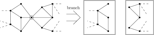
Figure 1: Branching on an articulation point (circled vertex) decomposes the graph into two connected components (gray boxes) that can be solved independently. The graphic shows the branch in which the vertex is excluded from the independent set.

Even though this strategy introduces only a small (linear) overhead, finding articulation points can be rare depending on the type of graph. This results in the default branching strategy being selected rather frequently. Furthermore, our preliminary experiments indicate that articulation points are rarely found at higher depth. However, due to their low overhead, we can justify searching for them whenever $A$ becomes empty.

4.2 Edge Cuts

To alleviate the restrictive nature of finding articulation points, we now propose a more flexible branching strategy based on (minimal) edge cuts. In general, we aim to find small vertex separators, i. e., a set of vertices whose removal disconnects the graph. We do so by making use of minimum edge cuts.

A cut $(S,T)$ is a partitioning of $V$ into two sets $S$ and $T=V\setminus S$. Furthermore, a cut is called minimum if its cut set $C=\{\{u,v\}\in E\mid u\in S,v\in T\}$ has minimal cardinality. However, in practice, finding minimum cuts often yields trivial cuts with either $S$ or $T$ only consisting of a single vertex with minimum degree. Thus, we are interested in finding $s$-$t$-cuts, i. e., cuts where $S$ and $T$ contain specific vertices $s,t\in V$. Finding these cuts can be done efficiently in practice, e. g., using a preflow push algorithm [17]. However, selecting the vertices $s$ and $t$ to ensure reasonably balanced cuts can be tricky. Natural choices include random vertices, as well as vertices that are far apart in terms of their shortest path distance. However, our preliminary experiments indicate that selecting random vertices of maximum degree for $s$ and $t$ seems to produce the best results. Finally, to derive a vertex separator from a cut, one can compute an MVC on the bipartite graph induced by the cut set, e. g., using the Hopcroft-Karp algorithm [22]. This separator can then be used to select branching vertices. In particular, we continuously branch on vertices from the separator.

Overall, our second strategy works similar to the first one: We maintain a set of possible branching vertices that were selected by computing a minimum $s$-$t$-cut and turning it into a vertex separator. Vertices that were removed by data reduction are discarded from this set and once it is empty a new cut computation is started. However, in contrast to the first strategy, finding a set of suitable branching vertices is much more likely. In order to avoid separators that contain too many vertices, and thus would require too many branching steps to disconnect the graph, we only keep those that do not exceed a certain size and balance threshold. The specific values for these threshold are presented in Section 6.2. Finally, if no suitable separator is found, we use the default branching strategy. Furthermore, in this case we do not try to find a new separator for a fixed number of branching steps as finding one is both unlikely and costly.

4.3 Nested Dissection

Both of our previous strategies dynamically maintain a set of branching vertices. Even though this comes at the advantage that most of the computed vertices remain viable candidates for some branching steps, it introduces a noticeable overhead. To alleviate this, our last strategy uses a static ordering of possible branching vertices that is computed once at the beginning of the algorithm. For this purpose we make use of a nested dissection ordering [16].

A nested dissection ordering of the vertices of a graph $G$ is obtained by recursively computing balanced bipartitions $(A,B)$ and a vertex separator $S$, that separates $A$ and $B$. The actual ordering is then given by concatenating the orderings of $A$ and $B$ followed by the vertices of $S$. Thus, if we select branching vertices based on the reverse of a nested dissection ordering, we continuously branch on vertices that disconnect the graph into balanced partitions. We compute such an ordering once, after finishing the initial data reduction phase.

There are two main optimizations that we use when considering the nested dissection ordering. First, we limit the number of recursive calls during the nested dissection computation, because we noticed that vertices at the end of the ordering seldom lead to a decomposition of the graph. This is due to the graph structure being changed by data reduction which can lead to separators becoming invalid. Furthermore, similar to the edge-cut-based strategy, we limit the size of separators considered during branching using a threshold. Again, this is done to ensure that we do not require too many branching steps to decompose the graph. The specific value for this size threshold is given in Section 6.2. If any separator in the nested dissection exceeds this threshold, we use the default branching strategy.

5 Reduction Branching

Our second approach to selecting good branching vertices is to choose a vertex whose removal will enable the application of new reduction rules. During every reduction step we find a list of candidate vertices to branch on. The following sections will demonstrate how we identify such branching candidate vertices with little computational overhead in practice. To be self contained we will also repeat the reduction rules used here but omit any proofs that can be found in the original publications. Out of the candidates found we then select a vertex of maximum degree. If the degree of all candidate vertices lies below a threshold (defined in Section 6.2) or no candidate vertices were found, we fall back to branching on a vertex of maximum degree. The rational here is that a vertex of large degree changes the structure of the graph more than a vertex of small degree even if that vertex is guaranteed to enable the application of a reduction rule. Also, our current strategies (except the packing-based rule in Section 5.4) only enable the application of the targeted reduction rule in the branch that excludes the vertex from the independent set, the excluding branch. However, in the case that includes it into the independent set (including branch) all neighbors are removed from the graph as well because they already have an adjacent vertex in the solution. Thus, in both branches multiple vertices are removed.

We also performed some preliminary experiments with storing the candidate vertices in a priority queue without resetting after every branch. However, changes were too frequent for this approach to be faster because of the high amount of priority queue operations.

5.1 Almost Twins

The first reduction we target is the twin reduction by Xiao and Nagamochi [38]:

Definition 5.1.

(Twins [38]) In a graph $G=(V,E)$ two vertices $u$ and $v$ are called twins if $N(u)=N(v)$ and $d(u)=d(v)=3$.

Theorem 5.2.

(Twin Reduction [38]) In a graph $G=(V,E)$ let vertices $u$ and $v$ be twins. If there is an edge among $N(u)$, then there is always an MIS that includes $\{u,v\}$ and therefore excludes $N(u)$. Otherwise, let $G^{\prime}=(V^{\prime},E^{\prime})$ be the graph with $V^{\prime}=(V\setminus N[\{u,v\}])\cup\{w\}$ where $w\notin V$ and $E^{\prime}=(E\cap\binom{V^{\prime}}{2})\cup\{\{w,x\}\;|\;x\in N^{2}(u)\}\}$ and let $I^{\prime}$ be an MIS in $G^{\prime}$. Then, $I=\begin{cases}I^{\prime}\cup\{u,v\}&\text{, if }w\notin I^{\prime}\\ (I^{\prime}\setminus\{w\})\cup N(u)&\text{, else}\end{cases}$ is an MIS in $G$.

We now define almost twins as follows:

Definition 5.3.

(Almost Twins) In a graph $G=(V,E)$ two non adjacent vertices $u$ and $v$ are called almost twins if $d(u)=4$, $d(v)=3$ and $N(v)\subseteq N(u)$ (i. e., $N(u)=N(v)\cup\{w\}$).

Clearly, after removing $w$, $u$ and $v$ are twins so we can apply the twin reduction. Finding almost twins can be done while searching for twins: The original algorithm checks for each vertex $v$ of degree-$3$ whether there is a vertex $u\in N^{2}(v)$ with $d(u)=3$ and $N(u)=N(v)$. We augment this algorithm by simultaneously also searching for $u\in N^{2}(v)$ with $d(u)=4$ and $N(v)\subset N(u)$. This induces about the same computational cost for degree-$4$ vertices in $N^{2}(v)$ as for degree $3$ vertices. While there might be instances where this causes high overhead, we expect the practical slowdown to be small. Figure 2 illustrates branching for almost twins.

Figure 2: Vertices $a$ and $b$ are almost twins. After branching on the circled vertex they become twins (in the excluding branch) and can be reduced.

5.2 Almost Funnels

Next, we consider the funnel reduction which is a special case of the alternative reduction by Xiao and Nagamochi [38]:

Definition 5.4.

(Alternative Sets [38]) In a graph $G=(V,E)$ two non empty, disjoint subsets $A,B\subseteq V$ are called alternatives if $|A|=|B|$ and there is an MIS $I$ in $G$ such that $I\cap(A\cup B)$ is either $A$ or $B$.

Theorem 5.5.

(Alternative Reduction [38]) In a graph $G=(V,E)$ let $A$ and $B$ be alternative sets. Let $G^{\prime}=(V^{\prime},E^{\prime})$ the graph with $V^{\prime}=V\setminus(A\cup B\cup(N(A)\cap N(B)))$ and $E^{\prime}=\{\{u,v\}\in E\mid u,v\in V^{\prime}\}\cup\{\{u,v\}\;|\;u\in N(A)\setminus N[B],v\in N(B)\setminus N[A]\}$ and let $I^{\prime}$ be an MIS in $G^{\prime}$. Then, $I=\begin{cases}I^{\prime}\cup A&\text{, if }(N(A)\setminus N[B])\cap I^{\prime}=\emptyset\\ I^{\prime}\cup B&\text{, else}\end{cases}$ is an MIS in $G$.

Note that the alternative reduction adds new edges between existing vertices of the graph which might not be beneficial in every case. To counteract this, the algorithm by Akiba and Iwata [1] only uses special cases, one of which is the funnel reduction:

Definition 5.6.

(Funnel [38]) In a graph $G=(V,E)$ two adjacent vertices $u$ and $v$ are called funnels if $G_{N(v)\setminus\{u\}}$ is a complete graph, i.e, if $N(v)\setminus\{u\}$ is a clique.

Theorem 5.7.

(Funnel Reduction [38]) In a graph $G=(V,E)$ let $u$ and $v$ be funnels. Then, $\{u\}$ and $\{v\}$ are alternative sets.

Again, we define a structure that is covered by the funnel reduction after removal of a single vertex:

Definition 5.8.

(Almost Funnel) In a graph $G=(V,E)$ two adjacent vertices $u$ and $v$ are called almost funnels if $u$ and $v$ are not funnels and there is a vertex $w$ such that $N(v)\setminus\{u,w\}$ induces a clique.

By removing $w$, $u$ and $v$ become funnels. The original funnel algorithm checks whether $u$ and $v$ are funnels by iterating over the vertices in $N(v)\setminus\{u\}$ and checking whether they are adjacent to all previous vertices. Once a vertex is found that is not adjacent to all previous vertices, the algorithm concludes that $u$ and $v$ are not funnels and terminates. We augment this algorithm by not immediately terminating in this case. Instead, we consider the following two cases: Either the current vertex $w$ is not adjacent to at least two of the previous vertices. In this case, we can check whether $N(v)\setminus\{u,w\}$ induces a clique. In the second case, $w$ is adjacent to all but one previous vertex $w^{\prime}$. In this case, both $w$ and $w^{\prime}$ might be candidate branching vertices. Thus, we check whether $N(v)\setminus\{u,w\}$ or $N(v)\setminus\{u,w^{\prime}\}$ induce a clique. This adds up to two additional clique checks (of slightly smaller size) to the one clique check in the original algorithm.

5.3 Almost Unconfined

The core idea of the unconfined reduction by Xiao and Nagamochi [38] is to detect vertices not required for an MIS that can therefore be removed from the graph by algorithmically contradicting the assumption that every MIS contains the vertex.

Definition 5.9.

(Child, Parent [38]) In a graph $G=(V,E)$ with an independent set $I$, a vertex $v$ is called a child of $I$ if $|N(v)\cap I|=1$ and the unique neighbor of $v$ in $I$ is called the parent of $v$.

Algorithm 1 shows the algorithm used by Akiba and Iwata [1] to detect so called unconfined vertices.

1

Input: A graph $G$, a vertex $v$

2 Unconfined(G, v) begin

3       $S\leftarrow\{v\}$

4       while $S\text{ has child }u\text{ with }|N(u)\setminus N[S]|\leq 1$ do

5             if $|N(u)\setminus N[S]|=0$ then

6                  return true

7            else

                   $\{w\}\leftarrow N(u)\setminus N[v]$

                    // by assumption $w$ also has to

                   $S\leftarrow S\cup\{w\}$

                    // be contained in every MIS

8                  

9            

10      

11      return false

12

Output: true if $v$ is unconfined, false otherwise

13

Algorithm 1 Unconfined – Xiao and Nagamochi [38]

Theorem 5.10.

(Unconfined Reduction [38]) In a graph $G=(V,E)$, if Algorithm 1 returns true for an unconfined vertex $v$, then there is always an MIS that does not contain $v$.

Again, we define a vertex to be almost unconfined:

Definition 5.11.

(Almost Unconfined) In a graph $G=(V,E)$ a vertex $v$ is called almost unconfined if $v$ is not unconfined but there is a vertex $w$ such that $v$ is unconfined in $G-\{w\}$.

Here, we only present an augmentation that detects some almost unconfined vertices. In particular, if at any point during the algorithm there is only one extending child, i.e. a child $u$ of $S$ with $N(u)\setminus N[S]=\{w\}$, then removal of $w$ makes $v$ unconfined. During Algorithm 1 we collect all these vertices $w$ and add them to the set of candidate branching vertices if the algorithm cannot already remove $v$. This only adds the overhead of temporarily storing the potential candidates and adding them to the actual candidate list if $v$ is not removed.

5.4 Almost Packing

The core idea behind the packing rule by Akiba and Iwata [1] is that when the exluding branch of a vertex $v$ is selected, one can assume that no maximum independent set contains $v$. Otherwise, if there is a maximum independent set that contains $v$, the algorithm finds it in the including branch of $v$. Based on the assumption that no maximum independent set includes a vertex $v$, constraints for the remaining vertices can be derived. For example, a maximum independent set that does not contain $v$ has to include at least two neighbors of $v$. The corresponding constraint is $\sum_{u\in N(v)}x_{u}\geq 2$, where $x_{u}$ is a binary variable that indicates whether a vertex is included in the current solution. Otherwise, we will find a solution of the same size in the branch including $v$. The algorithm creates such constraints when branching or reducing, and updates them accordingly during the data reductions and branching steps. When a vertex $v$ is eliminated from the graph, $x_{v}$ gets removed from all constraints. If $v$ is included into the current solution, the corresponding right sides are also decreased by one.

A constraint $\sum_{v\in S\subset V}x_{v}\geq k$ can be utilized in two reductions. Firstly, if $k$ is equal to the number of variables $|S|$, all vertices from $S$ have to be included into the current solution. If there are edges between vertices from $S$, then no valid solution can include all vertices from $S$, so the branch is pruned. Secondly, if there is a vertex $v$ such that $|S|-|N(v)\cap S|<k$, then $v$ has to be excluded from the current solution. If $k>|S|$, the constraint can not be fulfilled and the current branch is pruned.

In our branching strategy we target both reductions. If there is a constraint $\sum_{v\in S\subset V}x_{v}\geq k$, where $|S|=k+1$, excluding any vertex of $S$ from the solution or including a vertex of $S$ that has one neighbor in $S$ enables the first reduction. Thus, we consider all vertices in $S$ for branching. Note that including a vertex from $S$ that has more than one neighbor in $S$ makes the constraint unfulfillable and the branch is pruned.

If there is a constraint $\sum_{v\in S\subset V}x_{v}\geq k$ and a vertex $v$, such that $k=|S|-|N(v)\cap S|$, excluding any vertex of $S\setminus N(v)$ from the solution or including a vertex of $S\setminus N(v)$ that has at least one neighbor in $S\setminus N(v)$ enables the second reduction. Thus, we consider all vertices in $S\setminus N(v)$ for branching.

Note that in contrast to our previous reduction-based branching rules, packing reductions can also be applied in the including branch in many cases.

Detecting these branching candidates can be done with small constant overhead whilst performing the packing reduction.

6 Experimental Evaluation

In this section, we present the results of our experimental evaluation. Tables and figures here show aggregated results. For detailed results for all of our algorithms across all instances, see Appendix A.

6.1 Experimental Environment

We augment a C++-adaptation of the algorithm by Akiba and Iwata [1] with our branching strategies and compile it with g++ 9.3.0 using full optimizations (-O3). Our code is publicly available on GitHub. We execute all our experiments on a machine with 4 8-core Intel Xeon E5-4640 CPUs (2.4 GHz) and 512 GiB DDR3-PC1600 RAM running Ubuntu 20.04.1 with Linux Kernel 5.4.0-64. To speed up our experiments we use two identical machines and run at most 8 instances at once on the same machine (using the same machine for all algorithms on a specific instance). All numbers reported are arithmetic means of three runs with a timeout of ten hours.

6.2 Algorithm Configuration

We use a C++ adaptation of the implementation by Akiba and Iwata [1] in its default configuration as a basis for our algorithm. During preliminary experiments we found suitable values for the parameters of our techniques. These experiments were run on a subset of our total instance set. We use the geometric mean over all instances of the speedup over the default branching strategy as a basis for the following decisions: for the technique based on edge cuts, we only use cuts that contain at most 25 vertices and where the smaller side of the cut contains at least ten percent of the remaining vertices. If no suitable separator is found, we skip ten branching steps. For computing nested dissections, we use InertialFlowCutter [18] with the KaFFPa [34] backend. The KaFFPa partitioner is configured to use the strong preset with a fixed seed of $42$. For branching, we use three levels of nested dissections with a minimum balance of at least $40\%$ of the vertices in the smaller part of each dissection. Furthermore, we only use the nested dissection if separators contain at most 50 vertices. For the reduction-based branching rules, we fall back to the default branching strategy if all candidates have a degree of less than $\Delta-k$. In the case of twin-, funnel- and unconfined-reduction-based branching strategies we choose $k$ as $2$. For the packing-reduction-based branching rule, $k$ is set to $5$ and for the combined branching rule, $k$ is set to $4$.

6.3 Instances

We use instances from several sources: The “easy” instances used for the PACE 2019 Challenge on Minimum Vertex Cover [12]. Complements of Maximum Clique instances from the second DIMACS Implementation Challenge [23] and sparse instances from the Stanford Network Analysis Project (SNAP) [25], the 9th DIMACS Implementation Challenge on Shortest Paths [10] and the Network Data Repository [32]. Detailed instance information can be found in Table 1. Directed instances were converted into undirected graphs by ignoring the direction of edges and removing duplicates. Our original set of instances contained the first 80 PACE instances, 53 DIMACS instances and 34 sparse networks. From these instances, we excluded all instances that (1) required no branches, (2) on which all techniques had a running time of less than $0.1$ seconds, or (3) on which no technique was able to find a solution within 10 hours. The remaining set of instances is composed of 48 PACE instances, 37 DIMACS instances and 16 sparse networks.

Table 1: Number of vertices $|V|$ and edges $|E|$ for each graph.

PACE [12] instances:
Graph	$|V|$	$|E|$
05	200	798
06	200	733
10	199	758
16	153	802
19	200	862
31	200	813
33	4,410	6,885
35	200	864
36	26,300	41,500
37	198	808
38	786	14,024
39	6,795	10,620
40	210	625
41	200	1,023
42	200	952
43	200	841
44	200	1,147
45	200	1,020
46	200	812
47	200	1,093
48	200	1,025
49	200	933
50	200	1,025
51	200	1,098
52	200	992
53	200	1,026
54	200	961
55	200	938
56	200	1,089
57	200	1,160
58	200	1,171
59	200	961
60	200	1,118
61	200	931
62	199	1,128
63	200	1,011
64	200	1,042
65	200	1,011
66	200	866
67	200	1,174
68	200	961
69	200	1,083
70	200	860
71	200	952
72	200	1,167
73	200	1,078
74	200	805
77	200	961

DIMACS [23] instances:
Graph	$|V|$	$|E|$
C125.9	125	787
MANN_a27	378	702
MANN_a45	1,035	1,980
brock200_1	200	5,066
brock200_2	200	10,024
brock200_3	200	7,852
brock200_4	200	6,811
gen200_p0.9_44	200	1,990
gen200_p0.9_55	200	1,990
hamming8-4	256	11,776
johnson16-2-4	120	1,680
keller4	171	5,100
p_hat1000-1	1,000	377,247
p_hat1000-2	1,000	254,701
p_hat1500-1	1,500	839,327
p_hat300-1	300	33,917
p_hat300-2	300	22,922
p_hat300-3	300	11,460
p_hat500-1	500	93,181
p_hat500-2	500	61,804
p_hat500-3	500	30,950
p_hat700-1	700	183,651
p_hat700-2	700	122,922
san1000	1,000	249,000
san200_0.7_1	200	5,970
san200_0.7_2	200	5,970
san200_0.9_1	200	1,990
san200_0.9_2	200	1,990
san200_0.9_3	200	1,990
san400_0.5_1	400	39,900
san400_0.7_1	400	23,940
san400_0.7_2	400	23,940
san400_0.7_3	400	23,940
sanr200_0.7	200	6,032
sanr200_0.9	200	2,037
sanr400_0.5	400	39,816
sanr400_0.7	400	23,931

Sparse networks:
Graph	$|V|$	$|E|$	source
as-skitter	1,696,415	11,095,298	[25]
baidu-relatedpages	415,641	2,374,044	[32]
bay	321,270	397,415	[10]
col	435,666	521,200	[10]
fla	1,070,376	1,343,951	[10]
hudong-internallink	1,984,484	14,428,382	[32]
in-2004	1,382,870	13,591,473	[32]
libimseti	220,970	17,233,144	[32]
musae-twitch_DE	9,498	153,138	[25]
musae-twitch_FR	6,549	112,666	[25]
petster-fs-dog	426,820	8,543,549	[32]
soc-LiveJournal1	4,847,571	42,851,237	[25]
web-BerkStan	685,230	6,649,470	[25]
web-Google	875,713	4,322,051	[25]
web-NotreDame	325,730	1,090,108	[25]
web-Stanford	281,903	1,992,636	[25]

6.4 Decomposition Branching

Figure 3: Performance plots for decomposition-based branching strategies

Table 2: Speedup of our decomposition-based techniques over maximum degree branching.

	PACE	DIMACS	Sparse net.	All Instances
articulation points	0.99	0.99	2.17	1.20
edge cuts	1.00	0.99	2.29	1.22
nested dissections	1.00	0.99	2.15	1.21

Figure 3 shows performance profiles [11] of the running time and number of branches of our decomposition-based branching strategies: Let $\mathcal{T}$ be the set of all techniques we want to compare, $\mathcal{I}$ the set of instances, and $t_{T}({I})$ the running time/number of branches of technique $T\in\mathcal{T}$ on instance $I\in\mathcal{I}$. The y-axis shows for each technique $T$ the fraction of instances for which $t_{T}(I)\leq\tau\cdot\min_{T^{\prime}\in\mathcal{T}}t_{T^{\prime}}(I)$, where $\tau$ is shown on the x-axis. For $\tau=1$, the y-axis shows the fraction of instances on which a technique performs best. Note that these plots compare the performance of a technique relative to the best performing technique and do not show a ranking of all techniques. Instances that were not finished by a technique within the time limit are marked with ⏲.

The running time plot in Figure 3 shows that for most instances, the default strategy of branching on a vertex of maximum degree outperforms our decomposition-based approaches. However, for instances that have suitable candidates for decomposition, such as sparse networks, significant speedups compared to the default strategy can be seen. To be more specific, assigning a time of ten hours (our timeout threshold) for unfinished instances, we achieve a total speedup of $\numprint{2.15}$ to $\numprint{2.29}$ over maximum degree branching for our decomposition-based techniques on sparse networks (see Table 2). In particular, there is one instance (web-stanford) that causes a timeout with the default strategy but can be solved in $8$ (articulation points) to $43$ (nested dissections) seconds using a decomposition-based approach. Table 2 shows that overall, our technique using edge cuts seems to be the most beneficial, achieving an overall speedup of $22\%$ over maximum degree. Finally, Figure 3 shows that most running times are only slightly slower than the default strategy with a few instances showing a speedup. This is mainly because the number of branches required to solve the instances does not change in most cases and most of the running time difference is caused by the overhead from searching for branching vertices.

6.5 Reduction Branching

Figure 4 shows the performance profiles (see Section 6.4) for our reduction-based branching strategies. Here we see that targeting the packing reduction results in the fastest time for the most number of instances. In fact, targeting the packing reduction performs better than maximum degree branching on all but 3 PACE instances, achieving a speedup of $34\%$ (Table 3) on these instances. On the DIMACS instances, performance is closer to that of maximum degree with an overall speedup of $4\%$. On sparse networks, packing is only faster than maximum degree branching on $6$ out of $16$ instances but still achieves an overall speedup of $31\%$ due to being considerably faster on some of the longer running instances. The performance of our packing-based technique might be explained by it’s property of enabling a reduction in both the including and the excluding branch, while our other reduction-based techniques only enable a reduction in the excluding branch. Our funnel-based technique is faster than maximum degree branching for all but 4 of the PACE instances, resulting in a speedup of $14\%$ on these instances but only a $2\%$ speedup over all instances due to slightly slower running times on the other instance classes. We also show results for a strategy that targets all reduction rules described in Section 5 (called combined). Even though this approach leads to the second lowest number of branches for most instances, the time required to identify candidate vertices for all reduction rules causes too big of an overhead to be competitive. In fact, preliminary experiments showed that the number of branches is still small for a technique that only combines twin-, funnel- and unconfined-based branching. Optimizing the algorithms to identify candidate vertices could lead to making this combined strategy competitive.

Figure 4: Performance plots for reduction-based branching strategies

Table 3: Speedup of our reduction-based techniques over maximum degree branching.

	PACE	DIMACS	Sparse net.	All Instances
Twin	1.00	1.00	0.97	0.99
Funnel	1.14	0.99	0.98	1.02
Unconfined	0.79	1.00	0.86	0.92
Packing	1.34	1.04	1.31	1.16
Combined	1.14	1.03	1.30	1.12

7 Conclusion and Future Work

In this work we presented several novel branching strategies for the maximum independent set problem. Our strategies either follow a decomposition-based or reduction-rule-based approach. The decomposition-based strategies make use of increasingly sophisticated methods of finding vertices that are likely to decompose the graph into two or more connected components. Even though these strategies often come with a non negligible overhead, they work well for graphs that have a suitable structure, such as social networks. For instances that still favor the default branching strategy of branching on the vertex of highest degree, our reduction-rule-based strategies provide a smaller but more consistent speedup. These rules aim to facilitate the application of reduction rules which leads to smaller graphs that can be solved more quickly.

Overall, using one of our proposed strategies allows us to find the optimal solution the fastest for most instances tested. However, deciding which particular strategy to use for a given instance still remains an open problem. Finding suitable graph characteristics to do so provides an interesting opportunity for future work. Furthermore, our experimental evaluation on a combined approach that tries to use all reduction-rule-based strategies at the same time achieves a smaller number of branches than the default strategy for a large set of instances. However, the running time of this approach still suffers from frequent checks whether a particular vertex is a potential branching vertex. A more sophisticated and incremental way of tracking when a vertex becomes a branching vertex might provide significant performance benefits. In turn, this might lead to a branching strategy that consistently outperforms branching on the vertex of highest degree independent of the instance type.

Appendix A Detailed Experimental Results

We now present detailed results of our experimental evaluation. Detailed tables show running times $t$ (in seconds) and speedup $s$. Speedups are computed by dividing the running time of maximum degree branching by the running time of the respective technique. Timeouts are assigned a running time of ten hours. Note, that this is the same as our time limit. We also present the aggregated speedup $s_{\text{total}}$ computed by dividing the running time of both algorithms over all instances (omitting instances were both algorithms do not finish within our time limit). A value is highlighted in bold if it is the best one within a row.

Table 4: Detailed results for our decomposition-based strategies on the PACE instances.

Graph	max. deg.	articulation	edge cuts	nested dis.
PACE	t	t (s)	t (s)	t (s)
05	1.97	2.00 (0.98)	2.00 (0.99)	2.44 (0.81)
06	0.85	0.87 (0.98)	0.87 (0.98)	1.33 (0.64)
10	2.24	2.27 (0.99)	2.26 (0.99)	2.66 (0.84)
16	25,836.77	26,175.23 (0.99)	25,763.30 (1.00)	25,865.40 (1.00)
19	3.17	3.22 (0.98)	3.18 (0.99)	3.63 (0.87)
31	74.37	76.03 (0.98)	75.45 (0.99)	74.82 (0.99)
33	1.01	1.03 (0.98)	1.02 (0.99)	40.09 (0.03)
35	7.64	7.84 (0.97)	7.77 (0.98)	8.13 (0.94)
36	1.84	1.87 (0.98)	1.85 (0.99)	3.93 (0.47)
37	10.27	10.48 (0.98)	10.47 (0.98)	10.75 (0.96)
38	12.33	11.24 (1.10)	3.25 (3.79)	15.35 (0.80)
39	93.79	96.82 (0.97)	95.96 (0.98)	95.21 (0.99)
40	4,690.64	4,794.37 (0.98)	4,758.15 (0.99)	4,712.57 (1.00)
41	48.56	49.84 (0.97)	49.39 (0.98)	49.35 (0.98)
42	37.32	38.11 (0.98)	37.91 (0.98)	37.87 (0.99)
43	175.11	178.81 (0.98)	177.26 (0.99)	175.24 (1.00)
44	92.90	95.13 (0.98)	94.28 (0.99)	93.40 (0.99)
45	25.41	26.01 (0.98)	25.73 (0.99)	25.90 (0.98)
46	109.55	111.95 (0.98)	111.00 (0.99)	110.22 (0.99)
47	58.47	59.70 (0.98)	59.38 (0.98)	59.22 (0.99)
48	25.28	25.80 (0.98)	25.60 (0.99)	25.80 (0.98)
49	17.80	18.19 (0.98)	18.10 (0.98)	18.30 (0.97)
50	48.87	50.01 (0.98)	49.56 (0.99)	49.40 (0.99)
51	56.70	58.00 (0.98)	57.63 (0.98)	57.52 (0.99)
52	22.16	22.68 (0.98)	22.53 (0.98)	22.69 (0.98)
53	59.88	61.42 (0.97)	60.77 (0.99)	60.42 (0.99)
54	32.08	32.89 (0.98)	32.73 (0.98)	32.67 (0.98)
55	6.83	6.97 (0.98)	6.92 (0.99)	7.32 (0.93)
56	97.00	99.09 (0.98)	98.31 (0.99)	97.80 (0.99)
57	66.01	67.76 (0.97)	67.18 (0.98)	66.83 (0.99)
58	48.12	48.83 (0.99)	48.72 (0.99)	48.63 (0.99)
59	13.30	13.60 (0.98)	13.54 (0.98)	13.80 (0.96)
60	79.56	81.58 (0.98)	80.94 (0.98)	80.23 (0.99)
61	21.91	22.31 (0.98)	22.26 (0.98)	22.36 (0.98)
62	66.22	68.48 (0.97)	67.40 (0.98)	66.80 (0.99)
63	69.06	70.55 (0.98)	69.91 (0.99)	69.35 (1.00)
64	29.58	30.07 (0.98)	29.99 (0.99)	30.09 (0.98)
65	36.84	37.53 (0.98)	37.28 (0.99)	37.29 (0.99)
66	8.06	8.28 (0.97)	8.23 (0.98)	8.63 (0.93)
67	122.74	124.79 (0.98)	124.25 (0.99)	123.38 (0.99)
68	8.79	8.92 (0.99)	8.86 (0.99)	9.24 (0.95)
69	43.11	44.13 (0.98)	43.85 (0.98)	43.63 (0.99)
70	11.79	12.00 (0.98)	11.97 (0.99)	12.25 (0.96)
71	36.20	36.83 (0.98)	36.66 (0.99)	36.64 (0.99)
72	46.44	47.47 (0.98)	46.91 (0.99)	46.86 (0.99)
73	43.02	44.07 (0.98)	43.77 (0.98)	43.65 (0.99)
74	7.06	7.24 (0.97)	7.14 (0.99)	7.49 (0.94)
77	13.30	13.65 (0.97)	13.51 (0.98)	13.79 (0.96)
$s_{\text{total}}$	1.00	0.99	1.00	1.00

Table 5: Detailed results for our decomposition-based strategies on the DIMACS instances.

Graph	max. deg.	articulation	edge cuts	nested dis.
DIMACS	t	t (s)	t (s)	t (s)
C125.9	0.98	1.01 (0.97)	1.00 (0.98)	1.43 (0.69)
MANN_a27	0.48	0.49 (0.98)	0.49 (0.98)	0.98 (0.49)
MANN_a45	73.80	75.24 (0.98)	74.93 (0.98)	74.70 (0.99)
brock200_1	137.34	140.20 (0.98)	137.56 (1.00)	140.01 (0.98)
brock200_2	4.59	4.69 (0.98)	4.70 (0.98)	10.07 (0.46)
brock200_3	22.06	22.33 (0.99)	21.92 (1.01)	26.39 (0.84)
brock200_4	28.34	28.72 (0.99)	28.35 (1.00)	32.48 (0.87)
gen200_p0.9_44	152.61	156.30 (0.98)	154.50 (0.99)	153.49 (0.99)
gen200_p0.9_55	131.24	134.64 (0.97)	133.04 (0.99)	132.58 (0.99)
hamming8-4	19.29	19.65 (0.98)	19.49 (0.99)	25.38 (0.76)
johnson16-2-4	39.87	41.17 (0.97)	40.21 (0.99)	40.33 (0.99)
keller4	2.62	2.68 (0.98)	2.65 (0.99)	4.37 (0.60)
p_hat1000-1	860.24	868.71 (0.99)	870.04 (0.99)	906.24 (0.95)
p_hat1000-2	33,035.45	33,656.50 (0.98)	33,508.10 (0.99)	33,247.45 (0.99)
p_hat1500-1	8,935.77	9,015.15 (0.99)	9,015.74 (0.99)	8,994.28 (0.99)
p_hat300-1	3.70	3.79 (0.98)	3.82 (0.97)	23.94 (0.15)
p_hat300-2	5.53	5.66 (0.98)	5.63 (0.98)	21.76 (0.25)
p_hat300-3	189.58	191.06 (0.99)	188.96 (1.00)	196.89 (0.96)
p_hat500-1	38.63	39.26 (0.98)	39.41 (0.98)	59.29 (0.65)
p_hat500-2	96.36	97.82 (0.99)	97.58 (0.99)	107.29 (0.90)
p_hat500-3	14,860.70	14,895.15 (1.00)	14,979.65 (0.99)	14,909.35 (1.00)
p_hat700-1	163.30	162.84 (1.00)	163.17 (1.00)	177.34 (0.92)
p_hat700-2	906.32	917.87 (0.99)	914.96 (0.99)	917.50 (0.99)
san1000	895.34	902.64 (0.99)	903.38 (0.99)	920.28 (0.97)
san200_0.7_1	10.85	11.01 (0.98)	10.90 (1.00)	14.45 (0.75)
san200_0.7_2	0.33	0.34 (0.95)	0.32 (1.01)	2.34 (0.14)
san200_0.9_1	13.93	14.37 (0.97)	14.08 (0.99)	14.94 (0.93)
san200_0.9_2	34.15	34.77 (0.98)	34.35 (0.99)	34.90 (0.98)
san200_0.9_3	1,069.00	1,094.54 (0.98)	1,078.09 (0.99)	1,071.31 (1.00)
san400_0.5_1	9.21	9.35 (0.98)	9.36 (0.98)	16.76 (0.55)
san400_0.7_1	1,125.52	1,139.20 (0.99)	1,131.38 (0.99)	1,130.07 (1.00)
san400_0.7_2	3,062.38	3,053.97 (1.00)	3,083.59 (0.99)	3,073.66 (1.00)
san400_0.7_3	4,411.82	4,464.53 (0.99)	4,447.19 (0.99)	4,423.16 (1.00)
sanr200_0.7	48.35	49.51 (0.98)	48.71 (0.99)	52.13 (0.93)
sanr200_0.9	679.25	696.41 (0.98)	688.51 (0.99)	680.29 (1.00)
sanr400_0.5	373.40	374.20 (1.00)	374.26 (1.00)	380.08 (0.98)
sanr400_0.7	29,766.80	30,390.80 (0.98)	30,270.10 (0.98)	30,001.55 (0.99)
$s_{\text{total}}$	1.00	0.99	0.99	0.99

Table 6: Detailed results for our decomposition-based strategies on sparse networks.

Graph	max. deg.	articulation	edge cuts	nested dis.
Sparse net.	t	t (s)	t (s)	t (s)
as-skitter	2,058.32	2,100.57 (0.98)	2,071.06 (0.99)	2,068.46 (1.00)
baidu-relatedpages	0.82	0.88 (0.94)	0.86 (0.96)	7.22 (0.11)
bay	1.68	1.87 (0.90)	1.31 (1.28)	23.43 (0.07)
col	5,019.93	4,737.48 (1.06)	3,872.65 (1.30)	5,101.46 (0.98)
fla	25.33	23.47 (1.08)	24.58 (1.03)	329.42 (0.08)
hudong-internallink	0.99	1.55 (0.64)	1.46 (0.68)	1.99 (0.50)
in-2004	5.22	5.46 (0.96)	5.37 (0.97)	16.18 (0.32)
libimseti	1,497.59	1,507.54 (0.99)	1,503.49 (1.00)	1,704.53 (0.88)
musae-twitch_DE	20,906.93	21,470.00 (0.97)	20,987.30 (1.00)	20,949.83 (1.00)
musae-twitch_FR	37.13	37.81 (0.98)	37.32 (1.00)	41.55 (0.89)
petster-fs-dog	6.82	10.21 (0.67)	8.67 (0.79)	12.47 (0.55)
soc-LiveJournal1	9.87	11.50 (0.86)	11.06 (0.89)	23.91 (0.41)
web-BerkStan	134.22	360.88 (0.37)	138.84 (0.97)	207.92 (0.65)
web-Google	0.61	0.85 (0.71)	0.68 (0.89)	1.46 (0.41)
web-NotreDame	12.10	9.07 (1.33)	12.11 (1.00)	48.83 (0.25)
web-Stanford	>36,000	8.38 (>4,294.84)	27.41 (>1,313.18)	42.80 (>841.16)
$s_{\text{total}}$	1.00	2.17	2.29	2.15

Table 7: Detailed results for our reduction-based strategies on the PACE instances.

Graph	max. deg.	Twin	Funnel	Unconfined	Packing	Combined
PACE	t	t (s)	t (s)	t (s)	t (s)	t (s)
05	1.97	1.96 (1.01)	1.99 (0.99)	2.04 (0.97)	1.66 (1.19)	2.11 (0.93)
06	0.85	0.85 (1.00)	0.74 (1.15)	0.92 (0.92)	0.67 (1.27)	0.81 (1.05)
10	2.24	2.23 (1.01)	2.23 (1.00)	2.32 (0.97)	1.88 (1.19)	2.06 (1.09)
16	25,836.77	25,856.57 (1.00)	22,446.13 (1.15)	34,642.13 (0.75)	18,511.88 (1.40)	22,590.78 (1.14)
19	3.17	3.14 (1.01)	2.90 (1.09)	3.25 (0.98)	2.60 (1.22)	3.04 (1.04)
31	74.37	74.31 (1.00)	58.14 (1.28)	73.23 (1.02)	55.99 (1.33)	54.11 (1.37)
33	1.01	1.01 (1.00)	1.15 (0.88)	1.14 (0.89)	1.02 (0.99)	1.29 (0.79)
35	7.64	7.63 (1.00)	7.37 (1.04)	7.90 (0.97)	6.54 (1.17)	7.75 (0.99)
36	1.84	1.86 (0.99)	11.44 (0.16)	162.22 (0.01)	1.90 (0.97)	75.52 (0.02)
37	10.27	10.31 (1.00)	10.27 (1.00)	10.63 (0.97)	8.21 (1.25)	10.90 (0.94)
38	12.33	12.36 (1.00)	11.08 (1.11)	11.40 (1.08)	11.44 (1.08)	10.05 (1.23)
39	93.79	93.99 (1.00)	32.43 (2.89)	127.32 (0.74)	93.99 (1.00)	98.25 (0.95)
40	4,690.64	4,689.28 (1.00)	4,285.37 (1.09)	4,530.07 (1.04)	4,176.59 (1.12)	4,131.79 (1.14)
41	48.56	48.42 (1.00)	42.00 (1.16)	48.66 (1.00)	36.87 (1.32)	38.74 (1.25)
42	37.32	37.19 (1.00)	35.69 (1.05)	37.60 (0.99)	28.55 (1.31)	36.07 (1.03)
43	175.11	174.63 (1.00)	158.08 (1.11)	172.91 (1.01)	130.75 (1.34)	154.96 (1.13)
44	92.90	92.97 (1.00)	82.64 (1.12)	94.37 (0.98)	69.68 (1.33)	90.20 (1.03)
45	25.41	25.37 (1.00)	25.29 (1.01)	26.20 (0.97)	19.83 (1.28)	26.38 (0.96)
46	109.55	109.47 (1.00)	92.61 (1.18)	108.01 (1.01)	79.76 (1.37)	82.72 (1.32)
47	58.47	58.18 (1.00)	53.01 (1.10)	59.16 (0.99)	42.32 (1.38)	52.28 (1.12)
48	25.28	25.21 (1.00)	22.65 (1.12)	25.72 (0.98)	18.56 (1.36)	22.93 (1.10)
49	17.80	17.76 (1.00)	16.43 (1.08)	19.02 (0.94)	12.97 (1.37)	16.18 (1.10)
50	48.87	48.90 (1.00)	46.07 (1.06)	49.75 (0.98)	37.70 (1.30)	47.09 (1.04)
51	56.70	56.58 (1.00)	51.45 (1.10)	57.63 (0.98)	43.45 (1.31)	50.32 (1.13)
52	22.16	22.12 (1.00)	20.56 (1.08)	22.99 (0.96)	15.78 (1.40)	20.82 (1.06)
53	59.88	59.88 (1.00)	54.78 (1.09)	60.43 (0.99)	46.87 (1.28)	55.74 (1.07)
54	32.08	32.02 (1.00)	29.29 (1.10)	32.89 (0.98)	26.55 (1.21)	27.76 (1.16)
55	6.83	6.80 (1.00)	6.50 (1.05)	6.99 (0.98)	5.23 (1.31)	6.35 (1.08)
56	97.00	96.45 (1.01)	88.78 (1.09)	98.09 (0.99)	70.18 (1.38)	81.46 (1.19)
57	66.01	65.97 (1.00)	57.60 (1.15)	65.90 (1.00)	49.95 (1.32)	52.45 (1.26)
58	48.12	47.74 (1.01)	45.82 (1.05)	48.56 (0.99)	35.94 (1.34)	46.62 (1.03)
59	13.30	13.30 (1.00)	12.73 (1.04)	13.72 (0.97)	10.61 (1.25)	12.30 (1.08)
60	79.56	79.36 (1.00)	71.73 (1.11)	80.70 (0.99)	59.65 (1.33)	71.85 (1.11)
61	21.91	21.91 (1.00)	20.47 (1.07)	22.28 (0.98)	17.50 (1.25)	21.06 (1.04)
62	66.22	66.18 (1.00)	59.16 (1.12)	67.83 (0.98)	49.87 (1.33)	59.64 (1.11)
63	69.06	68.81 (1.00)	61.23 (1.13)	70.81 (0.98)	53.40 (1.29)	58.65 (1.18)
64	29.58	29.38 (1.01)	26.96 (1.10)	29.46 (1.00)	22.35 (1.32)	26.78 (1.10)
65	36.84	36.72 (1.00)	33.42 (1.10)	37.93 (0.97)	28.23 (1.30)	31.17 (1.18)
66	8.06	8.06 (1.00)	7.47 (1.08)	8.21 (0.98)	6.21 (1.30)	7.97 (1.01)
67	122.74	122.34 (1.00)	113.33 (1.08)	123.58 (0.99)	95.55 (1.28)	112.43 (1.09)
68	8.79	8.75 (1.00)	8.92 (0.99)	8.94 (0.98)	6.69 (1.31)	8.57 (1.03)
69	43.11	43.11 (1.00)	38.46 (1.12)	44.18 (0.98)	33.88 (1.27)	39.86 (1.08)
70	11.79	11.73 (1.00)	10.09 (1.17)	12.22 (0.96)	9.71 (1.21)	9.76 (1.21)
71	36.20	35.91 (1.01)	32.22 (1.12)	35.37 (1.02)	27.23 (1.33)	33.39 (1.08)
72	46.44	46.18 (1.01)	41.66 (1.11)	46.68 (0.99)	36.28 (1.28)	41.86 (1.11)
73	43.02	43.00 (1.00)	40.38 (1.07)	43.77 (0.98)	31.91 (1.35)	43.51 (0.99)
74	7.06	7.06 (1.00)	6.67 (1.06)	7.86 (0.90)	5.48 (1.29)	6.96 (1.01)
77	13.30	13.25 (1.00)	12.74 (1.04)	13.80 (0.96)	10.61 (1.25)	12.31 (1.08)
$s_{\text{total}}$	1.00	1.00	1.14	0.79	1.34	1.14

Table 8: Detailed results for our reduction-based strategies on the DIMACS instances.

Graph	max. deg.	Twin	Funnel	Unconfined	Packing	Combined
DIMACS	t	t (s)	t (s)	t (s)	t (s)	t (s)
C125.9	0.98	0.98 (1.00)	0.92 (1.07)	0.98 (1.00)	0.85 (1.15)	0.91 (1.08)
MANN_a27	0.48	0.48 (1.00)	0.57 (0.85)	0.52 (0.92)	0.48 (1.01)	0.59 (0.82)
MANN_a45	73.80	73.76 (1.00)	83.81 (0.88)	78.58 (0.94)	71.86 (1.03)	85.47 (0.86)
brock200_1	137.34	136.98 (1.00)	140.15 (0.98)	137.32 (1.00)	135.14 (1.02)	138.64 (0.99)
brock200_2	4.59	4.60 (1.00)	4.71 (0.98)	4.59 (1.00)	4.58 (1.00)	4.70 (0.98)
brock200_3	22.06	21.78 (1.01)	22.38 (0.99)	21.85 (1.01)	21.76 (1.01)	22.46 (0.98)
brock200_4	28.34	28.15 (1.01)	29.09 (0.97)	28.16 (1.01)	28.25 (1.00)	29.24 (0.97)
gen200_p0.9_44	152.61	152.40 (1.00)	136.94 (1.11)	169.47 (0.90)	132.81 (1.15)	149.63 (1.02)
gen200_p0.9_55	131.24	131.20 (1.00)	125.61 (1.04)	127.51 (1.03)	102.10 (1.29)	50.64 (2.59)
hamming8-4	19.29	19.30 (1.00)	19.78 (0.98)	19.12 (1.01)	19.35 (1.00)	19.67 (0.98)
johnson16-2-4	39.87	39.79 (1.00)	41.63 (0.96)	41.40 (0.96)	38.70 (1.03)	43.09 (0.93)
keller4	2.62	2.62 (1.00)	2.68 (0.98)	2.63 (1.00)	2.58 (1.02)	2.65 (0.99)
p_hat1000-1	860.24	859.74 (1.00)	870.92 (0.99)	873.91 (0.98)	862.77 (1.00)	871.60 (0.99)
p_hat1000-2	33,035.45	33,314.15 (0.99)	32,999.15 (1.00)	32,812.80 (1.01)	30,913.22 (1.07)	31,202.52 (1.06)
p_hat1500-1	8,935.77	8,935.50 (1.00)	9,009.69 (0.99)	8,954.18 (1.00)	8,958.19 (1.00)	9,046.97 (0.99)
p_hat300-1	3.70	3.69 (1.00)	3.78 (0.98)	3.69 (1.00)	3.68 (1.00)	3.78 (0.98)
p_hat300-2	5.53	5.53 (1.00)	5.68 (0.97)	5.54 (1.00)	5.48 (1.01)	5.63 (0.98)
p_hat300-3	189.58	187.77 (1.01)	189.16 (1.00)	185.68 (1.02)	175.01 (1.08)	179.53 (1.06)
p_hat500-1	38.63	38.70 (1.00)	39.36 (0.98)	39.03 (0.99)	38.61 (1.00)	39.34 (0.98)
p_hat500-2	96.36	96.39 (1.00)	97.87 (0.98)	96.21 (1.00)	95.08 (1.01)	96.96 (0.99)
p_hat500-3	14,860.70	14,887.15 (1.00)	14,624.90 (1.02)	14,765.90 (1.01)	13,429.92 (1.11)	13,712.38 (1.08)
p_hat700-1	163.30	160.75 (1.02)	163.63 (1.00)	160.81 (1.02)	163.24 (1.00)	163.31 (1.00)
p_hat700-2	906.32	908.46 (1.00)	914.56 (0.99)	906.78 (1.00)	866.08 (1.05)	879.99 (1.03)
san1000	895.34	898.16 (1.00)	906.21 (0.99)	901.40 (0.99)	913.29 (0.98)	932.29 (0.96)
san200_0.7_1	10.85	10.78 (1.01)	11.01 (0.99)	10.91 (0.99)	10.93 (0.99)	11.06 (0.98)
san200_0.7_2	0.33	0.32 (1.04)	0.33 (0.98)	0.31 (1.07)	0.32 (1.01)	0.33 (0.99)
san200_0.9_1	13.93	13.90 (1.00)	13.35 (1.04)	4.94 (2.82)	12.03 (1.16)	12.13 (1.15)
san200_0.9_2	34.15	33.87 (1.01)	21.46 (1.59)	12.32 (2.77)	15.80 (2.16)	10.01 (3.41)
san200_0.9_3	1,069.00	1,068.17 (1.00)	1,016.33 (1.05)	639.01 (1.67)	843.40 (1.27)	600.71 (1.78)
san400_0.5_1	9.21	9.21 (1.00)	9.37 (0.98)	9.13 (1.01)	9.24 (1.00)	9.37 (0.98)
san400_0.7_1	1,125.52	1,121.99 (1.00)	1,146.32 (0.98)	1,125.12 (1.00)	1,132.10 (0.99)	1,151.14 (0.98)
san400_0.7_2	3,062.38	3,063.23 (1.00)	3,066.62 (1.00)	3,463.29 (0.88)	3,048.94 (1.00)	3,489.72 (0.88)
san400_0.7_3	4,411.82	4,405.26 (1.00)	4,487.18 (0.98)	4,398.18 (1.00)	4,497.81 (0.98)	4,521.80 (0.98)
sanr200_0.7	48.35	48.34 (1.00)	50.09 (0.97)	48.41 (1.00)	48.49 (1.00)	50.25 (0.96)
sanr200_0.9	679.25	679.65 (1.00)	633.59 (1.07)	664.95 (1.02)	531.48 (1.28)	567.49 (1.20)
sanr400_0.5	373.40	370.59 (1.01)	376.93 (0.99)	377.71 (0.99)	370.72 (1.01)	376.10 (0.99)
sanr400_0.7	29,766.80	29,838.40 (1.00)	30,466.35 (0.98)	29,844.65 (1.00)	29,473.60 (1.01)	30,242.80 (0.98)
$s_{\text{total}}$	1.00	1.00	0.99	1.00	1.04	1.03

Table 9: Detailed results for our reduction-based strategies on sparse networks.

Graph	max. deg.	Twin	Funnel	Unconfined	Packing	Combined
Sparse net.	t	t (s)	t (s)	t (s)	t (s)	t (s)
as-skitter	2,058.32	2,054.41 (1.00)	1,849.79 (1.11)	1,977.94 (1.04)	1,681.87 (1.22)	1,704.73 (1.21)
baidu-relatedpages	0.82	0.80 (1.02)	0.84 (0.97)	0.85 (0.97)	0.83 (0.98)	0.93 (0.88)
bay	1.68	1.68 (1.00)	8.22 (0.20)	4.71 (0.36)	1.89 (0.89)	8.38 (0.20)
col	5,019.93	5,752.08 (0.87)	5,416.72 (0.93)	8,187.80 (0.61)	9,370.05 (0.54)	5,924.10 (0.85)
fla	25.33	25.41 (1.00)	45.62 (0.56)	76.60 (0.33)	34.78 (0.73)	42.75 (0.59)
hudong-internallink	0.99	1.31 (0.76)	1.27 (0.78)	1.21 (0.82)	1.55 (0.64)	1.12 (0.88)
in-2004	5.22	4.88 (1.07)	5.25 (0.99)	10.85 (0.48)	5.50 (0.95)	10.73 (0.49)
libimseti	1,497.59	1,452.17 (1.03)	1,620.09 (0.92)	1,440.71 (1.04)	1,476.25 (1.01)	1,706.07 (0.88)
musae-twitch_DE	20,906.93	20,996.87 (1.00)	21,190.67 (0.99)	22,650.53 (0.92)	19,345.03 (1.08)	23,006.50 (0.91)
musae-twitch_FR	37.13	37.04 (1.00)	38.58 (0.96)	41.15 (0.90)	35.60 (1.04)	42.46 (0.87)
petster-fs-dog	6.82	6.62 (1.03)	8.16 (0.84)	8.66 (0.79)	9.68 (0.70)	9.20 (0.74)
soc-LiveJournal1	9.87	6.64 (1.49)	9.57 (1.03)	9.49 (1.04)	11.33 (0.87)	10.69 (0.92)
web-BerkStan	134.22	135.47 (0.99)	122.30 (1.10)	146.94 (0.91)	123.60 (1.09)	174.07 (0.77)
web-Google	0.61	0.53 (1.15)	0.69 (0.87)	0.68 (0.89)	0.78 (0.78)	0.68 (0.89)
web-NotreDame	12.10	12.63 (0.96)	15.23 (0.79)	12.38 (0.98)	14.09 (0.86)	17.52 (0.69)
web-Stanford	>36,000	>36,000	>36,000	>36,000	17,886.35 (>2.01)	17,989.97 (>2.00)
$s_{\text{total}}$	1.00	0.97	0.98	0.86	1.31	1.30

References

- [1] Takuya Akiba and Yoichi Iwata. Branch-and-reduce exponential/FPT algorithms in practice: A case study of vertex cover. Theoretical Computer Science, 609:211–225, 2016. doi:10.1016/j.tcs.2015.09.023.
- [2] Maram Alsahafy and Lijun Chang. Computing maximum independent sets over large sparse graphs. In International Conference on Web Information Systems Engineering, pages 711–727. Springer, 2020.
- [3] Nicolas Bourgeois, Bruno Escoffier, Vangelis Th. Paschos, and Johan M. M. van Rooij. Fast algorithms for max independent set. Algorithmica, 62(1-2):382–415, 2012. doi:10.1007/s00453-010-9460-7.
- [4] Sergiy Butenko and Wilbert E Wilhelm. Clique-detection models in computational biochemistry and genomics. European Journal of Operational Research, 173(1):1–17, 2006.
- [5] Randy Carraghan and Panos M. Pardalos. An exact algorithm for the maximum clique problem. Operations Research Letters, 9(6):375–382, 1990. doi:10.1016/0167-6377(90)90057-C.
- [6] Lijun Chang, Wei Li, and Wenjie Zhang. Computing A near-maximum independent set in linear time by reducing-peeling. In Proceedings of the 2017 ACM International Conference on Management of Data, pages 1181–1196. ACM, 2017. doi:10.1145/3035918.3035939.
- [7] Jianer Chen, Iyad A. Kanj, and Ge Xia. Improved upper bounds for vertex cover. Theoretical Computer Science, 411(40-42):3736–3756, 2010. doi:10.1016/j.tcs.2010.06.026.
- [8] Tammy M. K. Cheng, Yu-En Lu, Michele Vendruscolo, Pietro Liò, and Tom L. Blundell. Prediction by graph theoretic measures of structural effects in proteins arising from non-synonymous single nucleotide polymorphisms. PLoS Computational Biology, 4(7), 2008. doi:10.1371/journal.pcbi.1000135.
- [9] Jakob Dahlum, Sebastian Lamm, Peter Sanders, Christian Schulz, Darren Strash, and Renato F Werneck. Accelerating local search for the maximum independent set problem. In International symposium on experimental algorithms, pages 118–133. Springer, 2016.
- [10] Camil Demetrescu, Andrew V Goldberg, and David S Johnson. The Shortest Path Problem: Ninth DIMACS Implementation Challenge, volume 74. American Mathematical Soc., 2009.
- [11] Elizabeth D Dolan and Jorge J Moré. Benchmarking optimization software with performance profiles. Mathematical programming, 91(2):201–213, 2002.
- [12] M. Ayaz Dzulfikar, Johannes K. Fichte, and Markus Hecher. The PACE 2019 Parameterized Algorithms and Computational Experiments Challenge: The Fourth Iteration. In 14th International Symposium on Parameterized and Exact Computation (IPEC 2019), volume 148, pages 25:1–25:23, 2019. doi:10.4230/LIPIcs.IPEC.2019.25.
- [13] Fedor V. Fomin, Fabrizio Grandoni, and Dieter Kratsch. A measure & conquer approach for the analysis of exact algorithms. J. ACM, 56(5):25:1–25:32, 2009. doi:10.1145/1552285.1552286.
- [14] Jian Gao, Jiejiang Chen, Minghao Yin, Rong Chen, and Yiyuan Wang. An exact algorithm for maximum k-plexes in massive graphs. In IJCAI, pages 1449–1455, 2018.
- [15] M. R. Garey, D. S. Johnson, and L. Stockmeyer. Some Simplified NP-Complete Problems. In Proceedings of the 6th ACM Symposium on Theory of Computing, STOC ’74, pages 47–63. ACM, 1974.
- [16] Alan George. Nested dissection of a regular finite element mesh. SIAM Journal on Numerical Analysis, 10(2):345–363, 1973.
- [17] Andrew V Goldberg and Robert E Tarjan. A new approach to the maximum-flow problem. Journal of the ACM (JACM), 35(4):921–940, 1988.
- [18] Lars Gottesbüren, Michael Hamann, Tim Niklas Uhl, and Dorothea Wagner. Faster and better nested dissection orders for customizable contraction hierarchies. Algorithms, 12(9):196, 2019.
- [19] Demian Hespe, Sebastian Lamm, Christian Schulz, and Darren Strash. Wegotyoucovered: The winning solver from the PACE 2019 challenge, vertex cover track. In Proceedings of the SIAM Workshop on Combinatorial Scientific Computing, pages 1–11. SIAM, 2020. doi:10.1137/1.9781611976229.1.
- [20] Demian Hespe, Christian Schulz, and Darren Strash. Scalable kernelization for maximum independent sets. Journal of Experimental Algorithmics (JEA), 24(1):1–22, 2019.
- [21] John Hopcroft and Robert Tarjan. Algorithm 447: efficient algorithms for graph manipulation. Communications of the ACM, 16(6):372–378, 1973.
- [22] John E Hopcroft and Richard M Karp. An n^5/2 algorithm for maximum matchings in bipartite graphs. SIAM Journal on computing, 2(4):225–231, 1973.
- [23] David S Johnson. Cliques, coloring, and satisfiability: second dimacs implementation challenge. DIMACS series in discrete mathematics and theoretical computer science, 26:11–13, 1993.
- [24] Tim Kieritz, Dennis Luxen, Peter Sanders, and Christian Vetter. Distributed time-dependent contraction hierarchies. In Experimental Algorithms, 9th International Symposium, volume 6049, pages 83–93. Springer, 2010. doi:10.1007/978-3-642-13193-6\_8.
- [25] Jure Leskovec and Andrej Krevl. SNAP Datasets: Stanford large network dataset collection. http://snap.stanford.edu/data, June 2014.
- [26] Chu-Min Li, Zhiwen Fang, and Ke Xu. Combining maxsat reasoning and incremental upper bound for the maximum clique problem. In 25th IEEE International Conference on Tools with Artificial Intelligence, pages 939–946. IEEE Computer Society, 2013. doi:10.1109/ICTAI.2013.143.
- [27] Chu-Min Li, Hua Jiang, and Felip Manyà. On minimization of the number of branches in branch-and-bound algorithms for the maximum clique problem. Computers & Operations Research, 84:1–15, 2017. doi:10.1016/j.cor.2017.02.017.
- [28] Chu-Min Li, Hua Jiang, and Ruchu Xu. Incremental maxsat reasoning to reduce branches in a branch-and-bound algorithm for maxclique. In Learning and Intelligent Optimization - 9th International Conference, volume 8994, pages 268–274. Springer, 2015. doi:10.1007/978-3-319-19084-6\_26.
- [29] Chu Min Li and Zhe Quan. An efficient branch-and-bound algorithm based on maxsat for the maximum clique problem. In Proceedings of the Twenty-Fourth AAAI Conference on Artificial Intelligence. AAAI Press, 2010.
- [30] Rick Plachetta and Alexander van der Grinten. Sat-and-reduce for vertex cover: Accelerating branch-and-reduce by sat solving. In 2021 Proceedings of the Workshop on Algorithm Engineering and Experiments (ALENEX), pages 169–180. SIAM, 2021.
- [31] Deepak Puthal, Surya Nepal, Cécile Paris, Rajiv Ranjan, and Jinjun Chen. Efficient algorithms for social network coverage and reach. In IEEE International Congress on Big Data, pages 467–474. IEEE Computer Society, 2015. doi:10.1109/BigDataCongress.2015.75.
- [32] Ryan A. Rossi and Nesreen K. Ahmed. The network data repository with interactive graph analytics and visualization. In AAAI, 2015. URL: http://networkrepository.com.
- [33] Pedro V. Sander, Diego Nehab, Eden Chlamtac, and Hugues Hoppe. Efficient traversal of mesh edges using adjacency primitives. ACM Trans. Graph., 27(5):144, 2008. doi:10.1145/1409060.1409097.
- [34] Peter Sanders and Christian Schulz. Think locally, act globally: Highly balanced graph partitioning. In Experimental Algorithms, 12th International Symposium, SEA 2013, Rome, Italy, June 5-7, 2013. Proceedings, volume 7933, pages 164–175. Springer, 2013.
- [35] Christian Schorr. Improved branching strategies for maximum independent sets. Master’s thesis, Karlsruhe Institute of Technology, 2020.
- [36] Pablo San Segundo and Cristóbal Tapia. Relaxed approximate coloring in exact maximum clique search. Computers & Operations Research, 44:185–192, 2014. doi:10.1016/j.cor.2013.10.018.
- [37] Etsuji Tomita, Yoichi Sutani, Takanori Higashi, and Mitsuo Wakatsuki. A simple and faster branch-and-bound algorithm for finding a maximum clique with computational experiments. IEICE Trans. Inf. Syst., 96-D(6):1286–1298, 2013. doi:10.1587/transinf.E96.D.1286.
- [38] Mingyu Xiao and Hiroshi Nagamochi. Confining sets and avoiding bottleneck cases: A simple maximum independent set algorithm in degree-3 graphs. Theoretical Computer Science, 469:92–104, 2013. doi:10.1016/j.tcs.2012.09.022.
- [39] Mingyu Xiao and Hiroshi Nagamochi. Exact algorithms for maximum independent set. Inf. Comput., 255:126–146, 2017. doi:10.1016/j.ic.2017.06.001.