A new distance measure of Pythagorean fuzzy sets based on matrix and and its application in medical diagnosis

Abstract

The pythagorean fuzzy set (PFS) which is developed based on intuitionistic fuzzy set, is more efficient in elaborating and disposing uncertainties in indeterminate situations, which is a very reason of that PFS is applied in various kinds of fields. How to measure the distance between two pythagorean fuzzy sets is still an open issue. Mnay kinds of methods have been proposed to present the of the question in former reaserches. However, not all of existing methods can accurately manifest differences among pythagorean fuzzy sets and satisfy the property of similarity. And some other kinds of methods neglect the relationship among three variables of pythagorean fuzzy set. To addrees the proplem, a new method of measuring distance is proposed which meets the requirements of axiom of distance measurement and is able to indicate the degree of distinction of PFSs well. Then some numerical examples are offered to to verify that the method of measuring distances can avoid the situation that some counter-intuitive and irrational results are produced and is more effective, reasonable and advanced than other similar methods. Besides, the proposed method of measuring distances between PFSs is applied in a real environment of application which is the medical diagnosis and is compared with other previous methods to demonstrate its superiority and efficiency. And the feasibility of the proposed method in handling uncertainties in practice is also proved at the same time.
keywords:  Pythagorean fuzzy set  Similarity measure
Distance measure  Pattern recognition  Medical diagnosis

I Introduction

There is lots of uncertain things existing in the real world, and how to measure the level of uncertainty has attracted incremental attention and interests from researches all around the world [1, 2, 3, 4, 5]. Therefore, many mathematic theory and models have been proposed to be applied into practical application, such as evidence theory [6, 7, 8, 9], belief function [10, 11, 12, 13, 14, 15, 16], belief structure [17, 18, 19, 20], probability assignment [21, 22, 23, 24, 25, 26], entropy theory [27, 28, 29, 30, 31, 32, 33], $Z$ numbers [34, 35, 36, 37] and $D$ numbers [38, 39, 40, 41, 42, 43], which are palying important roles in respects of people’s life. Except for these instruments mentioned above, an efficient tool to handle uncertainty called fuzzy set is introduced by Zadeh [44, 45], which is more operable in seeking for useful information among uncertainties and becomes a key component of pattern recognition [46, 47, 48, 13, 49] and decision making [50, 51, 52, 53]. According to the original definition of fuzzy set, an universe of discourse $U$ is given, a mapping from $U$ to an unit range $0$ to $1$ is called a fuzzy set and the value of the element in the mapping represent the membership. To some extent, the fuzzy set can manifest real condition relatively well.

However, when judging actual situations in real world, things are getting more complex, which indicates that a single value can not reflect the essence of certain objects. Therefore, a further concept based on the fuzzy set is propposed whose name is intuitionistic fuzzy set. And it is developed by Atanassov [54] and defined to contain $3$ elements, namely membership, non-membership and hesitance, which is obviously convenient in expressing reality and more intuitive. As a reinforced generation of fuzzy set, the intuitionistic fuzzy set is considered more efficient in handling ambiguity and deduces appropriate targets to be selected. And it is further developed in different fields, such as interval-valued intuitionistic fuzzy set [55, 56], quantum decision [57] and so on. Later on, a new extension is invented by Yager [58] which is called the pythagorean fuzzy set. The new concept derived from intuitionistic fuzzy set is a quadratic form of the former fuzzy set, which means that the new modality of fuzzy set has a larger range of the change of variables and therefore has more potential in indicating the probability of various objects. The new form of fuzzy set is also extended into different forms, such as interval-valued pythagorean fuzzy set [51], decision making [59, 60, 61] and some other applications [62] To simplify appellations of kinds of fuzzy set, intuitionistic fuzzy set is called IFS and pythagorean fuzzy set is named PFS.

No matter which kind of fuzzy set is discussed about, how to measure the differences or distances among fuzzy sets is an unavoidable problem. If the degree of differences can be transformed in to the value of numbers, it is much more convenient to solving problems which occur in dscision making, pattern recognition and medical diagnosis. In order to manifest the distances properly, many methods of measuring distances have been proposed and some of them have ideal effect in classification. The most widely used method of measuring distances between IFSs are the Hamming distance [63], Euclidean distance [63], the Hausdorff metric [64], Own’s distance [65], De et al.’s distance [66], Szmidt et al.’s distance [67], Wei et al.’s distance [55], Mondal et al’s distance [68] and so on. However, not all of the methods can produce intuitive results under any circumstances and may be obviously conflicting with data given. And because PFS is a generation of IFS, the method of measuring distance between IFSs can be rationally extended into the forms which can measure distance between PFSs. But some similar results produced are still not satisfying and intuitive enough.

Therefore, in this paper, a new method of measuring distance of PFSs is proposed. This method transforms the elements contained in the PFSs into a form of vector to maximize the role every element plays in generating distances. More than that, a newly defined matrix is utlized to strengthen the membership and non-membership and a reduction of the index of hesitance is alsi required so that a better performance in pattern recognition can be achieved. Compared with the results produced by other methods, the ones from the new proposed method is obviously more accurate and conforms to reality, which indicates it may be more efficient in practical application.

The rest of the paper is organized as follows. In the part of preliminaries, some relative concepts are briefly introduced. Besides, some previous methods of measuring distacnes and the proofs of their properties are also presented. Next, in the part of proposed method, every detail of it is clearly explained and some simple cases are offered to make the statements of the proposed method more straightforward. Moreover, some proofs of the properties required are also provided in this part. And in the part of examples and applications, the correctness and validity of the new proposed method in measuring distance are verified. In the last part, some details and advantages of the new proposed method are concluded.

II Preliminaries

In this section, some concepts related to pythagorean fuzzy sets (PFS) are introduced.

II-A Intuitionistic fuzzy set

Let $A$ denote an IFS in a finite universe of discourse which is named $X$. And the mathematic form of IFS $A$ can be defined as [54]:

$$A=\{{(x,\mu(x),\nu(x))|x\in X}\}$$ (1)

Besides, the parameters satisfy

$$\mu(x):X\to[0,1]$$ (2)

and

$$\nu(x):X\to[0,1]$$ (3)

$\mu(x)$ is a representative of the degree of membership of $x\in X$ and $\nu(x)$ is a representative of the degree of non-membership of $x\in X$. And both of them meet the condition that:

$$0\leq\mu(x)+\nu(x)\leq 1$$ (4)

The hesitance function of an IFS $A$ in $X$ is defined as:

$$\pi(x)=1-\mu(x)-\nu(x)$$ (5)

The value of $\pi(x)$ can reflect the degree of hesitance of $x\in X$.

II-B Pythagorean fuzzy sets

Let $A$ denote an PFS in a finite universe of discourse which is named $X$. And the mathematic form of PFS $A$ can be defined as [58, 59, 60]:

$$A=\{{(x,A_{Y}(x),A_{N}(x))|x\in X}\}$$ (6)

Besides, the parameters satisfy

$$A_{Y}(x):X\to[0,1]$$ (7)

and

$$A_{N}(x):X\to[0,1]$$ (8)

$A_{Y}(x)$ is a representative of the degree of membership of $x\in X$ and $\nu(x)$ is a representative of the degree of non-membership of $x\in X$. And both of them meet the condition that:

$$0\leq A^{2}_{Y}(x)+A^{2}_{N}(x)\leq 1$$ (9)

The hesitance function of an PFS $A$ in $X$ is defined as:

$$A_{H}(x)=\sqrt{1-A^{2}_{Y}(x)-A^{2}_{N}(x)}$$ (10)

The value of $A_{H}(x)$ can reflect the degree of hesitance of $x\in X$.
Property 1 : Let $B$ and $C$ be two PFS of the finite universe of discourse $X$, then both of them satisfy [59, 60]: (1) $B\subseteq C\ if\ \forall x\in X\ B_{Y}(x)\leq C_{Y}(x)\ and\ B_{N}(x)\geq C_{N}(x)$
(2) $B=C\ if\ \forall x\in X\ B_{Y}(x)=C_{Y}(x)\ and\ B_{N}(x)=C_{N}(x)$
(3) $B\ \cap\ C=\{\langle x,min[B_{Y}(x),C_{Y}(x)],max[B_{N}(x),C_{N}(x)]\rangle\\ |x\in X\}$
(4) $B\ \cup\ C=\{\langle x,max[B_{Y}(x),C_{Y}(x)],min[B_{N}(x),C_{N}(x)]\rangle\\ |x\in X\}$
(5) $B\!\!\cdot\!\!C=\{\langle x,B_{Y}(x)C_{Y}(x),(B^{2}_{Y}(x)+C^{2}_{Y}(x)-B^{2}_{Y}(x)C^{2}_{Y}(x))^{\frac{1}{2}}\rangle|x\in X\}$
(6) $B^{n}=\{\langle x,B^{n}_{Y}(x),(1-(1-B^{2}_{N}(x)^{n}))^{\frac{1}{2}}\rangle|x\in X\}$ In the next part, some separate methods of measuring the distance between different IFSs and PFSs are briefly introduced. And some useful function is also mentioned, which is helpful in judging the validity of IFS and even PFS in its extended form.

II-C Different methods of measuring distance related to pythagorean fuzzy sets

1. The definition of Hamming distance which measures difference between IFSs $D$ and $E$ is written as [63]:

$$\begin{split}d_{Hm}(D,E)=\frac{1}{2}\cdot(|\mu_{D}(x)-\mu_{E}(x)|+\\ |\nu_{D}(x)-\nu_{E}(x)|+|\pi_{D}(x)-\pi_{E}(x)|)\end{split}$$ (11)

2. The definition of normalized Hamming distance which measures difference between IFSs $D$ and $E$ is written as [63]:

$$\begin{split}\widetilde{d}_{Hm}(D,E)=\frac{1}{2n}\cdot\sum_{i=1}^{n}(|\mu_{D}(x_{i})-\mu_{E}(x_{i})|+\\ |\nu_{D}(x_{i})-\nu_{E}(x_{i})|+|\pi_{D}(x_{i})-\pi_{E}(x_{i})|)\end{split}$$ (12)

3. The definition of Euclidean distance which measures difference between IFSs $D$ and $E$ is written as [63]:

$$d_{Eu}(D,E)=(\frac{1}{2}\cdot((\mu_{D}(x)-\mu_{E}(x))^{2}+$$ (13)

$$(\nu_{D}(x)-\nu_{E}(x))^{2}+(\pi_{D}(x)-\pi_{E}(x))^{2}))^{\frac{1}{2}}$$

4. The definition of normalized Euclidean distance which measures difference between IFSs $D$ and $E$ is written as [63]:

$$\widetilde{d}_{Eu}(D,E)=(\frac{1}{2n}\cdot\sum_{i=1}^{n}((\mu_{D}(x_{i})-\mu_{E}(x_{i}))^{2}+$$ (14)

$$(\nu_{D}(x_{i})-\nu_{E}(x_{i}))^{2}+(\pi_{D}(x_{i})-\pi_{E}(x_{i}))^{2}))^{\frac{1}{2}}$$

II-D Methods of measuring the distance of IFS extended to PFS and existing method

1. The definition of Hamming distance which measures difference between PFSs $F$ and $G$ is written as [69]:

$$\begin{split}D_{Hm}(F,G)=\frac{1}{2}\cdot(|F^{2}_{Y}(x)-G^{2}_{Y}(x)|+\\ |F^{2}_{N}(x)-G^{2}_{N}(x)|+|F^{2}_{H}(x)-G^{2}_{H}(x)|)\end{split}$$ (15)

2. The definition of normalized Hamming distance which measures difference between PFSs $F$ and $G$ is written as:

$$\begin{split}\widetilde{D}_{Hm}(F,G)=\frac{1}{2n}\cdot\sum_{i=1}^{n}(|F^{2}_{Y}(x)-G^{2}_{Y}(x)|+\\ |F^{2}_{N}(x)-G^{2}_{N}(x)|+|F^{2}_{H}(x)-G^{2}_{H}(x)|)\end{split}$$ (16)

3. The definition of Euclidean distance which measures difference between PFSs $F$ and $G$ is written as [69]:

$$D_{Eu}(F,G)=(\frac{1}{2}\cdot((F^{2}_{Y}(x)-G^{2}_{Y}(x))^{2}+$$ (17)

$$(F^{2}_{N}(x)-G^{2}_{N}(x))^{2}+(F^{2}_{H}(x)-G^{2}_{H}(x)))^{\frac{1}{2}}$$

4. The definition of normalized Euclidean distance which measures difference between PFSs $F$ and $G$ is written as:

$$\widetilde{D}_{Eu}(F,G)=(\frac{1}{2n}\cdot\sum_{i=1}^{n}((F^{2}_{Y}(x)-G^{2}_{Y}(x))^{2}+$$ (18)

$$(F^{2}_{N}(x)-G^{2}_{N}(x))^{2}+(F^{2}_{H}(x)-G^{2}_{H}(x))^{2}))^{\frac{1}{2}}$$

5. The definition of Chen’s distance which measures difference between PFSs $F$ and $G$ is written as [69]:

$$D_{C}(F,G)=[\frac{1}{2}\cdot(|F^{2}_{Y}(x)-G^{2}_{Y}(x)|^{\beta}+$$ (19)

$$|F^{2}_{N}(x)-G^{2}_{N}(x)|^{\beta}+|F^{2}_{H}(x)-G^{2}_{H}(x)|^{\beta})]^{\frac{1}{\beta}}$$

The parameter $\beta$ in Chen’s distance which satisfies the condition that $\beta\geq 1$. When $\beta$ = 1, the method of Chen degenerates to the method of Hamming distance. Besides, when $\beta$ = 2, the method of Chen degenerates to the method of Euclidean distance.
6. The definition of Chen’s distance which measures difference between PFSs $F$ and $G$ is written as:

$$\widetilde{D}_{C}(F,G)=[\frac{1}{2n}\cdot\sum_{i=1}^{n}(|F^{2}_{Y}(x)-G^{2}_{Y}(x)|^{\beta}+$$ (20)

$$|F^{2}_{N}(x)-G^{2}_{N}(x)|^{\beta}+|F^{2}_{H}(x)-G^{2}_{H}(x)|^{\beta})]^{\frac{1}{\beta}}$$

The parameter $\beta$ in Chen’s distance which satisfies the condition that $\beta\geq 1$. When $\beta$ = 1, the method of Chen degenerates to the method of Hamming distance. Besides, when $\beta$ = 2, the method of Chen degenerates to the method of Euclidean distance.
Notion : On the base of the method of measuring the distance between IFSs, all of the methods offered above have been extended to adapt to the situation that the distance between 2 PFSs is supposed to be measured. More Importantly, the extended method of measuring the distance between PFSs still conforms to the concept of normalization.

II-E Score function on IFS and its extension

1. A score function of IFS is initialized by Chen and Tan and it is utilized in the solution of problems which are produced in multi-attribute decision using intuitionistic sets. Let $A$ be an intuitionistc fuzzy set in the finite universe of discourse X, which is $\{x_{1},x_{2},...x_{n}\}$. And IFS $A$ is given as $A=\{\langle x,\mu(x),\nu(x)\}$. Besides, the score function $S_{A}$ is defined as [70]: $S_{A}(x_{i})=\mu(x)-\nu(x)$ The value of the formula illustrates a degree that whether the intuitionistic fuzzy sets is comfortable enough for decision makers to have a clear and straightforward expectation to actual situations. Obviously, the value of $\mu(x)$ gets larger, the smaller the value of $\nu(x)$ is going to be and the reliability of $x\in X$ gets greater, which means the value of $S_{A}(x_{i})$ gets bigger. Therefore, the value of score function $S_{A}(x_{i})$ can be regarded as a kind of level of support about the element $x\in X$. When $S_{A}(x_{i})>0$, it can concluded that it is more believable to classify $x$ as a component of $X$. When $S_{A}(x_{i})<0$, it can concluded that it is more believable to classify $x$ as a exception of $X$. More than that, the absolute value of the score function can manifest the situation of the degree of certainty of IFS. If the mass is getting bigger, then the IFS is more certain. If the mass is getting smaller, then the IFS is more uncertain. For example, let $A$ and $B$ be two PFSs and they are defined respectively as $A=\{\langle x,0.35,0.35\rangle\}$ and $B=\{\langle x,0.6,0.1\rangle\}$. What should be pointed out is that the degree of hesitance in these two IFSs is exactly identical. However, the IFS $B$ is more valuable and useful, because it offers more information and can clearly illustrate actual situations. And obviously, the values of $|S_{A}(x)=0|$ and $|S_{B}(x)=0.5|$ is exactly consistent with the conclusion mentionedd above. As a consequence  the absolute value of $S_{A}(x)$ can be utlized as an efficient method to measure the level of certainty of an IFS.
2. On the base of the definition of score function which is developed on the concept of intuitionistic fuzzy set, a new score function $SP$ is on the notion of pythagorean fuzzy set which is defined as: $SF_{A}(x_{i})=A_{Y}^{2}(x_{i})-A_{N}^{2}(x_{i})$ The extended formula of PFS plays a similar role in handling PFSs, like the role of the degraded score function based on IFS which has.

II-F Propeties of Chen’s method and the proof of them

Some of the propoties of Chen’s distance can be interpreted as follows:
Property 2 : Let $H$ and $I$ be two PFSs in the finite universe of discourse X, then both of them satisfy: (1) $\widetilde{D}_{C}(H,I)=0\ if\ A=B\ and\ A\in X,B\in X$
(2) $\widetilde{D}_{C}(H,I)=\widetilde{D}_{C}(I,H)\ and\ A\in X,B\in X$
(3) $0\leq\widetilde{D}_{C}(H,I)\leq 1\ and\ A\in X,B\in X$ As what have been mentioned above, Hamming distance and Euclidean distance are special cases of normalized Chen’s distance. Therefore, both of them are expected to meet the condition which Chen’s distance requires.
And the demonstration of properties of normalized Chen’s distance is offered as follows:
Proof 1 : Let $A$ and $B$ be two PFSs in the finite universe of discourse $X$, both of them are supposed to satisfy:
$\widetilde{D}_{C}(A,B)=0$
As a result, the attribute of $\widetilde{D}_{C}(A,B)$ should be considered in the definition of Chen’s distance that $[\frac{1}{2}\cdot(|F^{2}_{Y}(x)-G^{2}_{Y}(x)|^{\beta}+|F^{2}_{N}(x)-G^{2}_{N}(x)|^{\beta}+|F^{2}_{H}(x)-G^{2}_{H}(x)|^{\beta})]^{\frac{1}{\beta}}=0$ Therefore, it can be concluded that $|F^{2}_{Y}(x)-G^{2}_{Y}(x)|^{\beta}=0$
$|F^{2}_{N}(x)-G^{2}_{N}(x)|^{\beta}=0$
$|F^{2}_{H}(x)-G^{2}_{H}(x)|^{\beta}=0$ From the equations, the relationships between every two parameters can be obtained $F^{2}_{Y}(x)=G^{2}_{Y}(x)$
$F^{2}_{N}(x)=G^{2}_{N}(x)$
$F^{2}_{H}(x)=G^{2}_{H}(x)$ Hence, it comes to a conclusion that when $\widetilde{D}_{C}(A,B)=0$, PFS $A$ is equal to PFS $B$.
Proof 2 : Let $A$ and $B$ be two PFSs in the finite universe of discourse $X$, both of them are supposed to satisfy:
The distance between PFS $A$ and $B$ is presented as: $\widetilde{D}_{C}(A,B)=[\frac{1}{2n}\cdot\sum_{i=1}^{n}\limits(|A^{2}_{Y}(x)-B^{2}_{Y}(x)|^{\beta}+\\ |A^{2}_{N}(x)-B^{2}_{N}(x)|^{\beta}+|A^{2}_{H}(x)-B^{2}_{H}(x)|^{\beta})]^{\frac{1}{\beta}}$ Then the distance between PFS $B$ and $A$ is presented as: $\widetilde{D}_{C}(B,A)=[\frac{1}{2n}\cdot\sum_{i=1}^{n}\limits(|B^{2}_{Y}(x)-A^{2}_{Y}(x)|^{\beta}+\\ |B^{2}_{N}(x)-A^{2}_{N}(x)|^{\beta}+|B^{2}_{H}(x)-A^{2}_{H}(x)|^{\beta})]^{\frac{1}{\beta}}$ After comparing these two equations, it can be summarized that $\widetilde{D}_{C}(A,B)=\widetilde{D}_{C}(B,A)$ because $|A^{2}_{Y}(x)-B^{2}_{Y}(x)|^{\beta}=|B^{2}_{Y}(x)-A^{2}_{Y}(x)|^{\beta}$
$|A^{2}_{N}(x)-B^{2}_{N}(x)|^{\beta}=|B^{2}_{N}(x)-A^{2}_{N}(x)|^{\beta}$
$|A^{2}_{H}(x)-B^{2}_{H}(x)|^{\beta}=|B^{2}_{H}(x)-A^{2}_{H}(x)|^{\beta}$ Proof 3 : Let $A$ and $B$ be two PFSs in the finite universe of discourse $X$, both of them are supposed to satisfy: $\widetilde{D}_{C}(A,B)\\ =[\frac{1}{2n}\cdot\sum_{i=1}^{n}\limits(|A^{2}_{Y}(x)-B^{2}_{Y}(x)|^{\beta}+|A^{2}_{N}(x)-B^{2}_{N}(x)|^{\beta}\\ +|A^{2}_{H}(x)-B^{2}_{H}(x)|^{\beta})]^{\frac{1}{\beta}}\\ =[\frac{1}{2n}\cdot\sum_{i=1}^{n}\limits(|A^{2}_{Y}(x)-B^{2}_{Y}(x)|^{\beta}+|A^{2}_{N}(x)-B^{2}_{N}(x)|^{\beta}\\ +|(1-A^{2}_{Y}(x)-A^{2}_{N}(x))-(1-B^{2}_{Y}(x)-B^{2}_{N}(x))|^{\beta})]^{\frac{1}{\beta}}\\ =[\frac{1}{2n}\cdot\sum_{i=1}^{n}\limits(|A^{2}_{Y}(x)-B^{2}_{Y}(x)|^{\beta}+|A^{2}_{N}(x)-B^{2}_{N}(x)|^{\beta}\\ +|A^{2}_{Y}(x)-B^{2}_{Y}(x)+A^{2}_{N}(x)-B^{2}_{N}(x)|^{\beta})]^{\frac{1}{\beta}}\\ \leq[\frac{1}{2n}\cdot\sum_{i=1}^{n}\limits(|A^{2}_{Y}(x)-B^{2}_{Y}(x)+A^{2}_{N}(x)-B^{2}_{N}(x)|^{\beta}\\ +|A^{2}_{Y}(x)-B^{2}_{Y}(x)+A^{2}_{N}(x)-B^{2}_{N}(x)|^{\beta})]^{\frac{1}{\beta}}\\ =[\frac{1}{n}\cdot\sum_{i=1}^{n}\limits(|A^{2}_{Y}(x)-B^{2}_{Y}(x)+A^{2}_{N}(x)-B^{2}_{N}(x)|^{\beta})]^{\frac{1}{\beta}}$ From the definition of pythagorean fuzzy sets, it can be summed up that $0\leq A^{2}_{Y}(x)\leq 1$   $0\leq B^{2}_{Y}(x)\leq 1$
$0\leq A^{2}_{N}(x)\leq 1$   $0\leq B^{2}_{N}(x)\leq 1$
$0\leq(A^{2}_{Y}(x)+A^{2}_{N}(x))\leq 1$  $0\leq(B^{2}_{Y}(x)+B^{2}_{N}(x))\leq 1$ As a result, it can be easily calculated that $0\leq(|A^{2}_{Y}(x)-B^{2}_{Y}(x)+A^{2}_{N}(x)-B^{2}_{N}(x)|^{\beta})\leq 1$ According to the equation above, a further conclusion can be made $0\leq[\frac{1}{n}\cdot\sum_{i=1}^{n}\limits(|A^{2}_{Y}(x)-B^{2}_{Y}(x)+A^{2}_{N}(x)-B^{2}_{N}(x)|^{\beta})]^{\frac{1}{\beta}}\leq 1$ Therefore, it can be obtained that $0\leq\widetilde{D}_{C}(A,B)\leq 1$ All of the properties of Chen’s method of measuring distance and the ones which degenerates from it have been proven.

III Proposed method

How to measure the differences between PFSs is still an open issue which plays a crucial part in target recognition. In this part, a new proposed method of measuring the distance between PFSs which is developed by a method of measuring the distance between IFSs based on a similarity matrix. Besides, the proposed method not only takes the advantage of the previous method which handles IFSs, but also further improve the performance of the similarity matrix in managing the mass of membership, non-membership and the hesitance. Then, the properties of the new proposed method are inferred and proven. In numerical examples, the new proposed method of measuring distance between PFSs satifies the distance measure axiom and is more efficient in producing intuitive and rational results.

III-A The new method of measuring distance

Let $A$ and $B$ be two PFSs in the finite universe of discourse X, the new formula which produces distances is defined as follows:

$$D_{N}(A,B)=\sqrt{\frac{1}{n}\sum_{i=1}^{n}\frac{\vec{m_{i}}M(\vec{m_{i}}M)^{T}}{AB_{Y}+AB_{N}+AB_{H}}}$$ (21)

$$AB_{Y}=A^{4}_{Y}(x_{i})+B^{4}_{Y}(x_{i})$$ (22)

$$AB_{N}=A^{4}_{N}(x_{i})+B^{4}_{N}(x_{i})$$ (23)

$$AB_{H}=A^{4}_{H}(x_{i})+B^{4}_{H}(x_{i})$$ (24)

$$\vec{m_{i}}=(A^{2}_{Y}(x_{i})-B^{2}_{Y}(x_{i}),A^{2}_{N}(x_{i})-B^{2}_{N}(x_{i}),A^{2}_{H}(x_{i})-B^{2}_{H}(x_{i}))$$ (25)

However, the definition of the matrix $M$ is still not clear. The most important efficacy of the matrix is to adjust and optimize the mass of membership, non-membership and the hesitance. Adopting the index of hesitance as a parameter to generating distance between different PFSs is not straightforward and concise, because the index of hesitance itself is a kind of uncertainty, which is very difficult to clarify the relationship between different hesitance. And coincidently, there is some kind of relationship between the hesitance and membership and non-membership. For example, let $A$ and $B$ be two PFSs in the finite universe of discourse X, where PFS $A=\{\langle 0,0,1\rangle\}$ and PFS $B=\{\langle 0.51,0.49,0.706\rangle\}$. In PFS $A$, the index of hesitance is equal to 1, which indicates that PFS $A$ is totally uncertain. Besides, on the contrary, the index of hesitance of PFS $B$ is 0, it means there is no uncertainty or vagueness commonly. However, the mass of membership and non-membership is so close that it is very difficult to make reasonable decisions. But one thing can be pointed out, the index of hesitance is not independent of the other two parameters, namely membership and non-membership, which means all of them have a similarity under certain relationship and is already sufficiently demonstrated in examples provided. Therefore, considering the relationship among the parameters, a new matrix is developed which is based on the previously defined matrix [71].
And the definition of the new matrix M is written as follows:

$$M=\begin{pmatrix}1&0&0\\ 0&1&0\\ Y&N&H\end{pmatrix}$$ (26)

$$Y=\frac{(A^{2}_{Y}(x_{i})+B^{2}_{Y}(x_{i}))}{(A^{2}_{Y}(x_{i})+B^{2}_{Y}(x_{i})+A^{2}_{N}(x_{i})+B^{2}_{N}(x_{i}))}$$ (27)

$$N=\frac{(A^{2}_{N}(x_{i})+B^{2}_{N}(x_{i}))}{(A^{2}_{Y}(x_{i})+B^{2}_{Y}(x_{i})+A^{2}_{N}(x_{i})+B^{2}_{N}(x_{i}))}$$ (28)

$$H=\sqrt{1-Y^{2}-N^{2}}$$ (29)

The main idea of the definition is that because uncertainty can not accurately show the real situation, then the mass of index is supposed to be distributed to membership and non-membership according to their mass in different PFSs to strengthen their ability of identification and not to change the original conditions, which enlarges the useful amount of information of pythagorean fuzzy sets and is helpful in target recognition. Due to the distribution to membership and non-membership, an adjustment of the index of hesitance should also be considered. Therefore, considering the mathematic form of PFS, it is proposed that $H=\sqrt{1-Y^{2}-N^{2}}$ is adopted as the remaining amount of information after the distribution to membership and non-membership. The operation of reduction in the index of hesitance improves the degree of identification, which is very helpful in measuring the distance of PFSs.
Specific details about matrix : The new distance proposed in this parper is based on the transformation of vectors from 3 parameters in PFSs. However, thr role of the vector and matrix is not just showing the original mass of 3 parameters. What can be concluded is that membership and non-membership is independent of each other, so both of the parameters is considered as orthogonal. Though membership and non-membership are treated equally, the relationship between hesitance and the other 2 paramerters is not just orthogonal, but presents a kind of proportion in membership and non-membership. It also conforms to the operation of some methods which handles the uncertainties of multiple elements propositions in evidece theory and is closely related to fuzzy sets. For example, two PFS $A=\{\langle 0.6,0.6,0.529\rangle\}$ and PFS $B=\{\langle 0.3,0.3,0.905\rangle\}$ is given to explain the process of the proposed vector and the new matrix which adjust the distribution of 3 parameters. The process is presented as follows: $\vec{m_{i}}=(A^{2}_{Y}(x_{i})-B^{2}_{Y}(x_{i}),A^{2}_{N}(x_{i})-B^{2}_{N}(x_{i}),A^{2}_{H}(x_{i})-B^{2}_{H}(x_{i}))=(0.27,0.27,-0.54)$
$Y=\frac{(A^{2}_{Y}(x_{i})+B^{2}_{Y}(x_{i}))}{(A^{2}_{Y}(x_{i})+B^{2}_{Y}(x_{i})+A^{2}_{N}(x_{i})+B^{2}_{N}(x_{i}))}=\frac{0.6^{2}+0.3^{2}}{2(0.6^{2}+0.3^{2})}=0.5$
$N=\frac{(A^{2}_{N}(x_{i})+B^{2}_{N}(x_{i}))}{(A^{2}_{Y}(x_{i})+B^{2}_{Y}(x_{i})+A^{2}_{N}(x_{i})+B^{2}_{N}(x_{i}))}=\frac{0.6^{2}+0.3^{2}}{2(0.6^{2}+0.3^{2})}=0.5$
$H=\sqrt{1-Y^{2}-N^{2}}=0.707$
$\vec{m_{i}}\times\begin{pmatrix}1&0&0\\ 0&1&0\\ Y&N&H\end{pmatrix}\\ =(0.27,0.27,-0.54)\times\begin{pmatrix}1&0&0\\ 0&1&0\\ 0.5&0.5&0.707\end{pmatrix}=(0,0,0.3818)$ Then the construction of a crucial part of the numerator is completed.

III-B Demonstration of Properties of proposed method

In this part, many properties of the proposed method is verified, like symmetry and triangle inequality.
Proof 4 : The commutative property is verified in this proof. Let $A$ and $B$ be two PFSs in the finite universe of discourse X. Considering $D_{N}(A,B)$ and $D_{N}(B,A)$, two equations can be obtained, one is $D_{N}(A,B)=\sqrt{\frac{1}{n}\sum_{i=1}^{n}\limits\frac{\vec{m_{i}}M(\vec{m_{i}}M)^{T}}{AB_{Y}+AB_{N}+AB_{H}}}$
$AB_{Y}=A^{4}_{Y}(x_{i})+B^{4}_{Y}(x_{i})$
$AB_{N}=A^{4}_{N}(x_{i})+B^{4}_{N}(x_{i})$
$AB_{H}=A^{4}_{H}(x_{i})+B^{4}_{H}(x_{i})$
$\vec{m_{i}}=(A^{2}_{Y}(x_{i})-B^{2}_{Y}(x_{i}),A^{2}_{N}(x_{i})-B^{2}_{N}(x_{i}),A^{2}_{H}(x_{i})-B^{2}_{H}(x_{i}))$
$M=\begin{pmatrix}1&0&0\\ 0&1&0\\ Y&N&H\end{pmatrix}$
$Y=\frac{(A^{2}_{Y}(x_{i})+B^{2}_{Y}(x_{i}))}{(A^{2}_{Y}(x_{i})+B^{2}_{Y}(x_{i})+A^{2}_{N}(x_{i})+B^{2}_{N}(x_{i}))}$
$N=\frac{(A^{2}_{N}(x_{i})+B^{2}_{N}(x_{i}))}{(A^{2}_{Y}(x_{i})+B^{2}_{Y}(x_{i})+A^{2}_{N}(x_{i})+B^{2}_{N}(x_{i}))}$ the other one is $D_{N}(B,A)=\sqrt{\frac{1}{n}\sum_{i=1}^{n}\limits\frac{\vec{m_{i}}M(\vec{m_{i}}M)^{T}}{BA_{Y}+BA_{N}+BA_{H}}}$
$BA_{Y}=B^{4}_{Y}(x_{i})+A^{4}_{Y}(x_{i})$
$BA_{N}=B^{4}_{N}(x_{i})+A^{4}_{N}(x_{i})$
$BA_{H}=B^{4}_{H}(x_{i})+A^{4}_{H}(x_{i})$
$\vec{m_{i}}=(B^{2}_{Y}(x_{i})-A^{2}_{Y}(x_{i}),B^{2}_{N}(x_{i})-A^{2}_{N}(x_{i}),B^{2}_{H}(x_{i})-A^{2}_{H}(x_{i}))$
$M=\begin{pmatrix}1&0&0\\ 0&1&0\\ Y&N&H\end{pmatrix}$
$Y=\frac{B^{2}_{Y}(x_{i})+A^{2}_{Y}(x_{i})}{(B^{2}_{Y}(x_{i})+A^{2}_{Y}(x_{i})+B^{2}_{N}(x_{i})+A^{2}_{N}(x_{i}))}$
$N=\frac{B^{2}_{N}(x_{i})+A^{2}_{N}(x_{i})}{(B^{2}_{Y}(x_{i})+A^{2}_{Y}(x_{i})+B^{2}_{N}(x_{i})+A^{2}_{N}(x_{i}))}$ It can be easily concluded that, when PFS $A$ and $B$ interchange their places, the attributes $AB_{Y}$, $AB_{N}$, $AB_{H}$, matrix $M$, $Y$ and $N$ do not change their values. But how the numerator $\vec{m_{i}}M(\vec{m_{i}}M)^{T}$ change is not very clear. Nevertheless, it can be also easily proved like this: $\vec{m_{i}}M(\vec{m_{i}}M)^{T}$
$=(A^{2}_{Y}(x_{i})-B^{2}_{Y}(x_{i})+Y(A^{2}_{H}(x_{i})-B^{2}_{H}(x_{i})))^{2}\\ +(A^{2}_{N}(x_{i})-B^{2}_{N}(x_{i})+N(A^{2}_{H}(x_{i})-B^{2}_{H}(x_{i})))^{2}\\ +((B^{2}_{H}(x_{i})-A^{2}_{H}(x_{i}))(\sqrt{1-Y^{2}-N^{2}}))^{2}\\ =(B^{2}_{Y}(x_{i})-A^{2}_{Y}(x_{i})+Y(B^{2}_{H}(x_{i})-A^{2}_{H}(x_{i})))^{2}\\ +(B^{2}_{N}(x_{i})-A^{2}_{N}(x_{i})+N(B^{2}_{H}(x_{i})-A^{2}_{H}(x_{i})))^{2}\\ +((A^{2}_{H}(x_{i})-B^{2}_{H}(x_{i}))(\sqrt{1-Y^{2}-N^{2}}))^{2}$ Therefore, it is proved that the proposed method of measuring distance between PFSs satisfy the property that $D_{N}(A,B)=D_{N}(B,A)$.
Proof 5 : A simple example is offered to verify a basic attirbute that is when 2 PFSs are exactly the same, their distance is coincidently 0. Let $A$ and $B$ become two identical PFSs, namely $\{\langle 0.5,0.5,0.707\rangle\}$, their distance is supposed to be 0 intuitively. And according to the definition of the vector $\vec{m_{i}}$, every component in the vector is equal to 0, which means the numerator $\vec{m_{i}}M(\vec{m_{i}}M)^{T}$ of the method of measuring distance is exactly 0 and the value of the whole formula is also 0. Therefore,the distance of the proposed method satisfies the property that $D_{N}(A,B)=0$ if and only if $A=B$.
Proof 6 : In this proof, the distance between 2 PFSs is demonstrated that $0\leq D_{N}(A,B)\leq 1$. Let $A$ and $B$ be two PFSs in the finite universe of discourse X, then it can be obtained that $\vec{m_{i}}M\\ =(A^{2}_{Y}(x_{i})-B^{2}_{Y}(x_{i})+Y(A^{2}_{H}(x_{i})-B^{2}_{H}(x_{i})),\\ A^{2}_{N}(x_{i})-B^{2}_{N}(x_{i})+N(A^{2}_{H}(x_{i})-B^{2}_{H}(x_{i})),\\ (B^{2}_{H}(x_{i})-A^{2}_{H}(x_{i}))(\sqrt{1-Y^{2}-N^{2}})$
$\vec{m_{i}}M(\vec{m_{i}}M)^{T}\\ =(A^{2}_{Y}(x_{i})-B^{2}_{Y}(x_{i})+Y(A^{2}_{H}(x_{i})-B^{2}_{H}(x_{i})))^{2}\\ +(A^{2}_{N}(x_{i})-B^{2}_{N}(x_{i})+N(A^{2}_{H}(x_{i})-B^{2}_{H}(x_{i})))^{2}\\ +((B^{2}_{H}(x_{i})-A^{2}_{H}(x_{i}))(\sqrt{1-Y^{2}-N^{2}}))^{2}\\ =(A^{2}_{Y}(x_{i})-B^{2}_{Y}(x_{i}))^{2}+(A^{2}_{N}(x_{i})-B^{2}_{N}(x_{i}))^{2}\\ +(A^{2}_{H}(x_{i})-B^{2}_{H}(x_{i}))^{2}\\ +2Y(A^{2}_{Y}(x_{i})-B^{2}_{Y}(x_{i}))(A^{2}_{H}(x_{i})-B^{2}_{H}(x_{i}))\\ +2N(A^{2}_{N}(x_{i})-B^{2}_{N}(x_{i}))(A^{2}_{H}(x_{i})-B^{2}_{H}(x_{i}))\\ =A^{4}_{Y}(x_{i})+B^{4}_{Y}(x_{i})+A^{4}_{N}(x_{i})+B^{4}_{N}(x_{i})+A^{4}_{H}(x_{i})+B^{4}_{H}(x_{i})\\ -2A^{2}_{Y}(x_{i})B^{2}_{Y}(x_{i})-2A^{2}_{N}(x_{i})B^{2}_{N}(x_{i})-2A^{2}_{H}(x_{i})B^{2}_{H}(x_{i})\\ +(A^{2}_{H}(x_{i})-B^{2}_{H}(x_{i}))\\ ((2YA^{2}_{Y}(x_{i})+2NA^{2}_{N}(x_{i}))-(2YB^{2}_{Y}(x_{i})+2NB^{2}_{N}(x_{i})))\leq A^{4}_{Y}(x_{i})+B^{4}_{Y}(x_{i})+A^{4}_{N}(x_{i})+B^{4}_{N}(x_{i})+A^{4}_{H}(x_{i})+B^{4}_{H}(x_{i})$ Obviously, when the entirety of $2YA^{2}_{Y}(x_{i})+2NA^{2}_{N}(x_{i})$ is larger than $2YB^{2}_{Y}(x_{i})+2NB^{2}_{N}(x_{i})$’s, $A^{2}_{H}(x_{i})-B^{2}_{H}(x_{i})$ is definitely negative, according to the defintion of pythagorean fuzzy set. Vice versa. Therefore, it can be inferred that $0\leq\frac{\vec{m_{i}}M(\vec{m_{i}}M)^{T}}{A^{4}_{Y}(x_{i})+B^{4}_{Y}(x_{i})+A^{4}_{N}(x_{i})+B^{4}_{N}(x_{i})+A^{4}_{H}(x_{i})+B^{4}_{H}(x_{i})}\leq 1$

$0\leq\frac{1}{n}\sum_{i=1}^{n}\limits\frac{\vec{m_{i}}M(\vec{m_{i}}M)^{T}}{A^{4}_{Y}(x_{i})+B^{4}_{Y}(x_{i})+A^{4}_{N}(x_{i})+B^{4}_{N}(x_{i})+A^{4}_{H}(x_{i})+B^{4}_{H}(x_{i})}\leq 1$
Let $T=\frac{1}{n}\sum_{i=1}^{n}\limits\frac{\vec{m_{i}}M(\vec{m_{i}}M)^{T}}{A^{4}_{Y}(x_{i})+B^{4}_{Y}(x_{i})+A^{4}_{N}(x_{i})+B^{4}_{N}(x_{i})+A^{4}_{H}(x_{i})+B^{4}_{H}(x_{i})}$
Therefore, $0\leq\sqrt{T}\leq 1$ Because $\sqrt{T}$ has the same significance with $D_{n}(A,B)$. Then, it can be concluded that $0\leq D_{n}(A,B)\leq 1$.
Proof 7 : The trangle inequality is going to be proven in this part. Some assumptions are given as: $Assumption1:A_{Y}^{2}(x)\leq B_{Y}^{2}(x)\leq C_{Y}^{2}(x)$
$Assumption2:C_{Y}^{2}(x)\leq B_{Y}^{2}(x)\leq A_{Y}^{2}(x)$
$Assumption3:B_{Y}^{2}(x)\leq min\{A_{Y}^{2}(x),C_{Y}^{2}(x)\}$
$Assumption4:B_{Y}^{2}(x)\geq max\{A_{Y}^{2}(x),C_{Y}^{2}(x)\}$ It can be easily demonstrated that the inequality $|A_{Y}^{2}(x)-C_{Y}^{2}(x)|\leq|A_{Y}^{2}(x)-B_{Y}^{2}(x)|+|B_{Y}^{2}(x)-C_{Y}^{2}(x)|$ which meets condtions of Assumption 1 and Assumption 2.
On the base of Assumption 3, it can be concluded that $A_{Y}^{2}(x)\geq B_{Y}^{2}(x)$
$C_{Y}^{2}(x)\geq B_{Y}^{2}(x)$ Therefore, it can be obtained that $|A_{Y}^{2}(x)-B_{Y}^{2}(x)|+|B_{Y}^{2}(x)-C_{Y}^{2}(x)|-|A_{Y}^{2}(x)-C_{Y}^{2}(x)|\\ =f(x)=\left\{\begin{aligned} A_{Y}^{2}(x)-B_{Y}^{2}(x)+C_{Y}^{2}(x)-B_{Y}^{2}(x)-A_{Y}^{2}(x)\\ +C_{Y}^{2}(x)\ \ if\ A_{Y}^{2}(x)\geq C_{Y}^{2}(x)\\ A_{Y}^{2}(x)-B_{Y}^{2}(x)+C_{Y}^{2}(x)-B_{Y}^{2}(x)+A_{Y}^{2}(x)\\ -C_{Y}^{2}(x)\ \ if\ A_{Y}^{2}(x)\leq C_{Y}^{2}(x)\\ \end{aligned}\right.$

$=2\cdot(min\{A_{Y}^{2}(x),C_{Y}^{2}(x)\}-B_{Y}^{2}(x))\geq 0$ Homoplastically, on the base Assumption 4, it can be summarized that $|A_{Y}^{2}(x)-B_{Y}^{2}(x)|+|B_{Y}^{2}(x)-C_{Y}^{2}(x)|-|A_{Y}^{2}(x)-C_{Y}^{2}(x)|\\ =f(x)=\left\{\begin{aligned} B_{Y}^{2}(x)-A_{Y}^{2}(x)+B_{Y}^{2}(x)-C_{Y}^{2}(x)-A_{Y}^{2}(x)\\ +C_{Y}^{2}(x)\ \ if\ A_{Y}^{2}(x)\geq C_{Y}^{2}(x)\\ B_{Y}^{2}(x)-A_{Y}^{2}(x)+B_{Y}^{2}(x)-C_{Y}^{2}(x)+A_{Y}^{2}(x)\\ -C_{Y}^{2}(x)\ \ if\ A_{Y}^{2}(x)\leq C_{Y}^{2}(x)\\ \end{aligned}\right.$

$=2\cdot(B_{Y}^{2}(x)-max\{A_{Y}^{2}(x),C_{Y}^{2}(x)\})\geq 0$ Hence, the property of inequality $|A_{Y}^{2}(x)-C_{Y}^{2}(x)|\leq|A_{Y}^{2}(x)-B_{Y}^{2}(x)|+|B_{Y}^{2}(x)-C_{Y}^{2}(x)|$ is also satisfied under the condition provided by Assumption 3 and Assumption 4. And because every component in the method of measuring distance is correspondingly proportionable to membership, non-membership and the index of hesitance. As a result, the triangle inequality has been proved. It can be concluded that $D_{N}(A,B)+D_{N}(B,C)\geq D_{N}(A,C)$ All of the required properties of the proposed which are expected to be satisfied have been demonstrated. In the next part, some examples are offered to further verify the validity of proposed method.

IV Numerical examples and application

In this section, lots of numerical examples and actual applications are utilized to illustrate the effectiveness of the method proposed in this paper of measuring distances between PFSs. And the accuracy and superiority of this method is also testified in this part.

TABLE I: Distances generated by Euclidean’s method and proposed method

$The\ change\ of\ \delta^{\prime}s\ value$	$Distances$
	$Euclidean$	$proposed\ method$
$0.1$	$0.1$	$0.1048$
$0.2$	$0.1$	$0.1154$
$0.3$	$0.1$	$0.1259$
$0.4$	$0.1$	$0.1348$
$0.5$	$0.1$	$0.1400$
$0.6$	$0.1$	$0.1400$
$0.7$	$0.1$	$0.1348$
$0.8$	$0.1$	$0.1259$
$0.9$	$0.1$	$0.1154$
$1.0$	$0.1$	$0.1048$

TABLE II: The change of the value of score function

$\delta$	$0.1$	$0.2$	$0.3$	$0.4$	$0.5$	$0.6$	$0.7$	$0.8$	$0.9$	$1$
$S(A)$	$-0.8$	$-0.6$	$-0.4$	$-0.2$	$0$	$0.2$	$0.4$	$0.6$	$0.8$	$1$
$S(B)$	$-1$	$-0.8$	$-0.6$	$-0.4$	$-0.2$	$0$	$0.2$	$0.4$	$0.6$	$0.8$
$|S(A)|$	$0.8$	$0.6$	$0.4$	$0.2$	$0$	$0.2$	$0.4$	$0.6$	$0.8$	$1$
$|S(B)|$	$1$	$0.8$	$0.6$	$0.4$	$0.2$	$0$	$0.2$	$0.4$	$0.6$	$0.8$

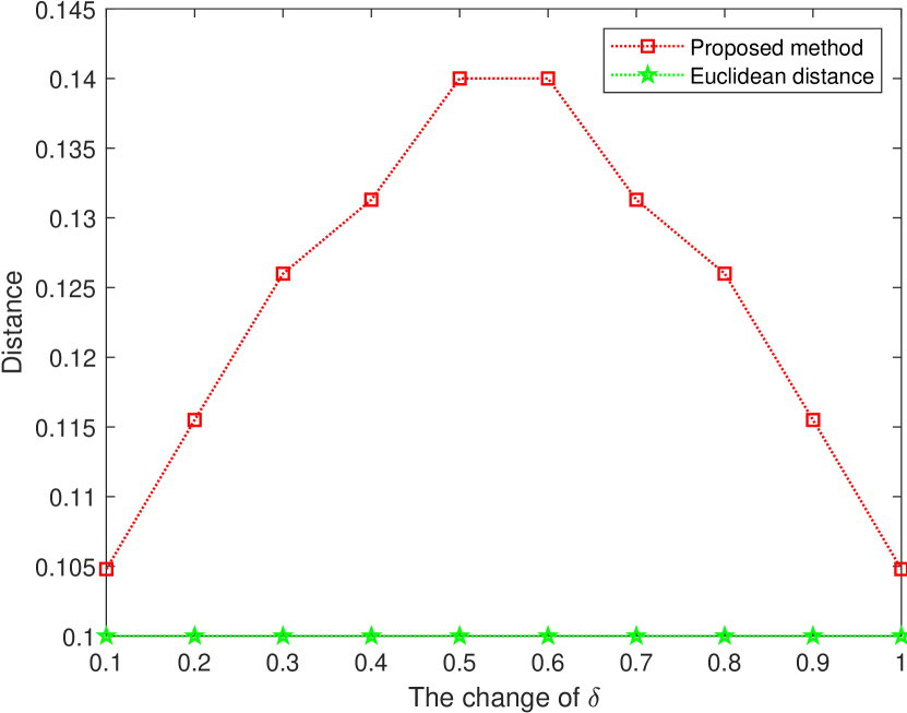
Figure 1:

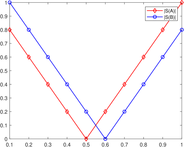
Figure 2:

TABLE III: Examples of PFSs

$PFSs$	$Case1$	$Case2$
$A_{i}$	$\{\langle{\color[rgb]{1,0,0}x_{1},0.55,0.45}\rangle,\langle{\color[rgb]{1,0,0}x_{2},0.63,0.55}\rangle\}$	$\{\langle{\color[rgb]{1,0,0}x_{1},0.55,0.45}\rangle,\langle{\color[rgb]{1,0,0}x_{2},0.63,0.55}\rangle\}$
$B_{i}$	$\{\langle x_{1},0.39,0.50\rangle,\langle x_{2},0.50,0.59\rangle\}$	$\{\langle x_{1},0.40,0.51\rangle,\langle x_{2},0.51,0.60\rangle\}$
$PFSs$	$Case3$	$Case4$
$A_{i}$	$\{\langle{\color[rgb]{0,0,1}x_{1},0.71,0.63}\rangle,\langle{\color[rgb]{0,0,1}x_{2},0.63,0.55}\rangle\}$	$\{\langle{\color[rgb]{0,0,1}x_{1},0.71,0.63}\rangle,\langle{\color[rgb]{0,0,1}x_{2},0.63,0.55}\rangle\}$
$B_{i}$	$\{\langle x_{1},0.63,0.63\rangle,\langle x_{2},0.71,0.63\rangle\}$	$\{\langle x_{1},0.77,0.55\rangle,\langle x_{2},0.55,0.45\rangle\}$
$PFSs$	$Case5$	$Case6$
$A_{i}$	$\{\langle{\color[rgb]{1,0,0}x_{1},0.55,0.45}\rangle,\langle{\color[rgb]{1,0,0}x_{2},0.63,0.55}\rangle\}$	$\{\langle{\color[rgb]{0,1,0}x_{1},0.30,0.20}\rangle,\langle{\color[rgb]{0,1,0}x_{2},0.40,0.30}\rangle\}$
$B_{i}$	$\{\langle x_{1},0.67,0.39\rangle,\langle x_{2},0.74,0.50\rangle\}$	$\{\langle x_{1},0.15,0.25\rangle,\langle x_{2},0.25,0.35\rangle\}$
$PFSs$	$Case7$	$Case8$
$A_{i}$	$\{\langle{\color[rgb]{0,1,0}x_{1},0.30,0.20}\rangle,\langle{\color[rgb]{0,1,0}x_{2},0.40,0.30}\rangle\}$	$\{\langle x_{1},0.50,0.40\rangle,\langle x_{2},0.40,0.30\rangle\}$
$B_{i}$	$\{\langle x_{1},0.45,0.15\rangle,\langle x_{2},0.55,0.25\rangle\}$	$\{\langle x_{1},0.40,0.40\rangle,\langle x_{2},0.50,0.40\rangle\}$

TABLE IV: Distances generated by different methods

$Methods$	$Case1$	$Case2$	$Case3$	$Case4$	$Case5$	$Case6$	$Case7$	$Case8$
$\widetilde{d}_{Hm}$	$0.1464$	$0.1351$	$0.1170$	$0.1350$	$0.1161$	$0.1500$	$0.1500$	$0.1500$
$\widetilde{d}_{Eu}$	$0.1298$	$0.1180$	$0.1110$	$0.1261$	$0.1009$	$0.1323$	$0.1323$	$0.1414$
$\widetilde{D}_{Hm}$	$0.1500$	$0.1400$	$0.1500$	$0.1500$	$0.1500$	$0.0825$	$0.1275$	$0.1250$
$\widetilde{D}_{Eu}$	$0.1323$	$0.1217$	$0.1414$	$0.1414$	$0.1323$	$0.0740$	$0.1186$	$0.1170$
$\widetilde{D}_{C}(\beta=1)$	$0.1500$	$0.1400$	$0.1500$	$0.1500$	$0.1500$	$0.0825$	$0.1275$	$0.1250$
$\widetilde{D}_{C}(\beta=2)$	$0.1323$	$0.1217$	$0.1414$	$0.1414$	$0.1323$	$0.0740$	$0.1186$	$0.1170$
$\widetilde{D}_{N}$	$0.1801$	$0.1756$	$0.1417$	$0.1517$	$0.1578$	$0.0746$	$0.0829$	$0.0982$

IV-A Examples and discussions

Example 1: Let $A$ and $B$ be two PFSs in the finite universe of discourse X, which are defined as $A=\{(x,A_{Y}(x),A_{N}(x))\}$ and $B=\{(x,B_{Y}(x),B_{N}(x))\}$. Besides, a further limitation is defined as: $A_{Y}^{2}(x)=\delta$
$A_{N}^{2}(x)=1-\delta$
$A_{Y}^{2}(x)=\delta-0.1$
$A_{N}^{2}(x)=1.1-\delta$
$A_{H}^{2}(x)=0=B_{H}^{2}(x)$ When setting the index of hesitance to 0, the difference between 2 PFSs is only about the values of membership and non-membership. The operation is carried to simplify the process of calculation. And of course, any parameter can be modified in this way, as long as the mass of each parameter satisfies the properties of pythagorean fuzzy set. And the differece of classic Euclidean distance and the new proposed is going to be discussed. All the results generated by the two methods are shown in table 1. And the values obtained by score function are also shown in table 2 with the consistent increase of the value of parameter $\delta$ which indicates a corresponding change in the distance of IFSs.

It can be easily told that the distance generated by classic Euclidean’s method is a fixed value. However, this phenonmenon is conflicting with the intuitive judgements. With the change of the $\delta$, if the results have not changed, then the results produced should be regarded irrational and counter-intuitive, which also indicates that the classic Euclidean distance is not sensitive to tiny variation among different PFSs. It may not accurately reveal potential changes in the relation of PFSs when they vary correspondingly but not symmetrically, which is crucial about whether a method of measuring distance can make reasonable judgements. Besides, when coming to analyse the variation of the variable $\delta$, the rationality and correctness of the proposed method is highlighted. With the increase of parameter $\delta$, when $\delta$ is in the range $0.1$ to $0.5$, the level of vagueness in these PFSs is getting higher, so the distance between two PFSs reaches its zenith. That is because the new proposed method can better detect the changes of different PFSs and present the difference in the results produced, which improved the sensitivity of distance measure compared to classic Euclidean distance. And the trend of the changes of PFSs can also be shown by the variation of the value of score function. While the parameter gradually reached the value of $0.5$, both of the absolute values of the score function of PFSs $A$ and $B$ are becoming smaller, which indicates the level of ambiguity of both PFSs is also getting higher. Because the PFSs are getting more uncertain, the distance between them is becoming bigger to indicate their distance can not be properly measured. Therefore, the new proposed method reflects this factor in the results and can better embody underlying relationship between or among PFSs.
Example 2: In this part, some numerical examples are given to illustrate the proority of new proposed method compared to other previous methods. Let $A_{i}$ and $B_{i}$ be two PFSs in the finite universe of discourse $X=\{x_{1},x_{2}\}$ and all of the docimastic cases are presented in table 3. And the distances generated by different methods are shown in table 4.
When coming to analysing the examples given in table 3, it can be easily concluded that $A_{1}=A_{2}=A_{5}$, but $B_{1}\neq B_{2}\neq B_{5}$; $A_{3}=A_{4}$, but $B_{3}\neq B_{4}$; $A_{6}=A_{7}$, but $B_{6}\neq B_{7}$. However, the results produced by different methods show a completely different figure among provided methods of measuring distances. After inspecting all of results, it can be summarized that:
1. After comparing all of the method of measuring distances between different PFSs, every method can accurately detect the differences under the condition in $Case1$ and $Case2$.
2. However, the results produced by $\widetilde{D}_{Hm}$, $\widetilde{D}_{Eu}$, $\widetilde{D}_{C}(\beta=1)$ and $\widetilde{D}_{C}(\beta=2)$ seem not satisfying. They produce the exactly the same results in completely different cases, which is counter-intuitive and irrational.
3. Besides, when checking the results produced by $\widetilde{d}_{Hm}$ and $\widetilde{d}_{Eu}$ in $Case6$ and $Case7$, they are also unreasonable due to the same results in different cases.
4. More than what have been mentioned in point $3$, $\widetilde{d}_{Hm}$ also dose not perform well in $Case7$ and $Case8$. Because the method produces another counter-intuitive results under different conditions.
5. All in all, when comparing all the cases mentioned above, it is very easy to distinguish that the distance of the new proposed method is more sensitive to the changes in PFSs and significantly indicates the discrimination level of different PFSs, which is much more efficient than any other methods. It is more rational and closer to actual situations.
6. A more important point should be noticed is that the new proposed method performs well under any cases given in the table 3 in producing distances between PFSs, which other ones generate irrational and counter-intuitive results in the same cases.

TABLE V: Properties different methods satisfy

$Methods$	$Properties$
	$Non-degeneracy$	$Symmetry$	$Triangleinequality$	$Boundness$
$\widetilde{d}_{Hm}$	$\surd$	$\surd$	$\surd$	$\surd$
$\widetilde{d}_{Eu}$	$\surd$	$\surd$	$\surd$	$\surd$
$\widetilde{D}_{Hm}$	$\surd$	$\surd$	$\surd$	$\surd$
$\widetilde{D}_{Eu}$	$\surd$	$\surd$	$\surd$	$\surd$
$\widetilde{D}_{C}(\beta=1)$	$\surd$	$\surd$	$\surd$	$\surd$
$\widetilde{D}_{C}(\beta=2)$	$\surd$	$\surd$	$\surd$	$\surd$
$\widetilde{D}_{N}$	$\surd$	$\surd$	$\surd$	$\surd$

Notice: It can be inferred from table 5 that except for the normalized Chen’s distance measure $\widetilde{D}_{C}$, other methods of measuring distances like $\widetilde{d}_{Hm}$, $\widetilde{d}_{Eu}$, $\widetilde{D}_{Hm}$, $\widetilde{D}_{Eu}$, $\widetilde{D}_{N}$ satisfy all the properties which the methods of distance measure are supposed to have. Moreover, the reason for the new proposed method can generate more rational and intuitive results is that the new proposed method considers discrepancies in PFSs and enlarges their influences in producing distances, which plays a significant role in manifesting differences. As a result, the new proposed method is more acceptable and conforms to acltual situations.

IV-B Applications and discussions

In this section, a new algorithm which is developed on the base of the new proposed method is designed for medical pattern recognition problems.
Problem narration : Assume there are a finite universe of discourse $X=\{x_{1},x_{2},x_{3},...,x_{n}\}$, existing medical patterns $P=\{P_{1},P_{2},P_{3},...,P_{k}\}$ consisting of n elements in the form of PFSs, expressed as $P_{j}=\{\langle x_{i},P_{Y}^{j}(x_{i}),P_{N}^{j}(x_{i})\}(1\leq j\leq k)$ in the finite universe of discourse $X$. And several examples $E=\{E_{1},E_{2},E_{3},...,E_{r}\}$ which is composed of $r$ samples is given to be rocognized and testify the correctness of the new algorithm. And all of the elements in example $E$ is denoted as the form of PFS and the whole example is written as $E_{u}=\{\langle x_{i},E_{Y}^{u}(x_{i}),E_{N}^{u}(x_{i})\}(1\leq u\leq r)$. All in all, what are expected to be achieved is to decide or classify every element in example $E_{u}$ whether belongs to the pattern $P_{j}$. The algorithm is designed as:
Step 1: For every element in $E_{u}$, the new proposed method of measuring distances is utlized to produce the distance between $P_{j}$ and $E_{u}$.

$D_{N}(P_{j},E_{u})=\sqrt{\frac{1}{n}\sum_{i=1}^{n}\frac{\vec{m_{i}}M(\vec{m_{i}}M)^{T}}{P_{j}E_{u}Y+P_{j}E_{u}N+P_{j}E_{u}H}}$

$P_{j}E_{u}Y=P_{j}^{4}{Y}(x_{i})+E_{u}^{4}{Y}(x_{i})$
$P_{j}E_{u}N=P_{j}^{4}{N}(x_{i})+E_{u}^{4}{N}(x_{i})$
$P_{j}E_{u}H=P_{j}^{4}{H}(x_{i})+E_{u}^{4}{H}(x_{i})$
$\vec{m_{i}}=(P_{j}^{2}{Y}(x_{i})-E_{u}^{2}{Y}(x_{i}),P_{j}^{2}{N}(x_{i})-E_{u}^{2}{N}(x_{i}),P_{j}^{2}{H}(x_{i})-E_{u}^{2}{H}(x_{i}))$
$M=\begin{pmatrix}1&0&0\\ 0&1&0\\ Y&N&H\end{pmatrix}$
$Y=\frac{(P_{j}^{2}{Y}(x_{i})+E_{u}^{2}{Y}(x_{i}))}{(P_{j}^{2}{Y}(x_{i})+E_{u}^{2}{Y}(x_{i})+P_{j}^{2}{N}(x_{i})+E_{u}^{2}{N}(x_{i}))}$
$N=\frac{(P_{j}^{2}{N}(x_{i})+E_{u}^{2}{N}(x_{i}))}{(P_{j}^{2}{Y}(x_{i})+E_{u}^{2}{Y}(x_{i})+P_{j}^{2}{N}(x_{i})+E_{u}^{2}{N}(x_{i}))}$
$H=\sqrt{1-Y^{2}-N^{2}}$ Step 2 : After calculating the distance of every pair of $P_{j}$ and $E_{u}$, the smallest value of the distances between two PFSs $P_{j}$ and $E_{u}$ is selected, which is written as: $\widetilde{D}_{N}^{choosen}=\mathop{min}\limits_{1\leq u\leq r}\widetilde{D}_{N}(P_{j},E_{u})$ Step 3 : According to the results generated by step 2, an element is classified into a pattern $P_{\beta}$, which is written as $\beta=arg\mathop{min}\limits_{1\leq u\leq r}\{\widetilde{D}_{N}(P_{j},E_{u})\}$
$E_{u}\leftarrow P_{\beta}$ In order to make the process of classifying more straightforward, a flow chart is offered as follows.
Except for that, the corresponding pseudocode is given in $Algorithm1$. And it can be easily concluded that the complexity of time of $Algorithm1$ is $O(n^{2})$, where n is a magnitude of certain problems.

Algorithm 1 :The details of the proposed algorithm

Input: The sets of every pattern $P=\{P_{1},P_{2},P_{3},...,P_{k}\}$
The sets of every sample $E=\{E_{1},E_{2},E_{3},...,E_{r}\}$
Output: The results of classification of samples $E_{u}$
$\textbf{for}\ j=1;\ j\leq k$  do
—– $\textbf{for}\ u=1;\ u\leq r$  do
———–Generate the distance $\widetilde{D}_{N}(P_{j},E_{u})$ between different PFSs by using the new proposed method
—– end       /- Step 1 -/
Choose the minimum value of $\widetilde{D}_{N}(P_{j},E_{u})$ as the final distance       /- Step 2 -/
Classify the tested sample $E_{u}$ into the corresponding pattern $P_{j}$       /- Step 3 -/
end

Example : To clarify the specific process of the algorithm, a simple is offered to illustrate details in handling data. Assume there are three medical patterns $P_{1}$, $P_{2}$ and $P_{3}$ which are expressed in the form of PFS in the finite universe of discourse $X=\{x_{1},x_{2},x_{3}\}$ and the details of the three medical patterns are written as follows: $P_{1}=\{\langle x_{1},0.4,0.7\rangle,\langle x_{2},0.5,0.6\rangle,\langle x_{2},0.7,0.4\rangle\}$
$P_{2}=\{\langle x_{1},0.6,0.7\rangle,\langle x_{2},0.4,0.5\rangle,\langle x_{2},0.9,0.1\rangle\}$
$P_{3}=\{\langle x_{1},0.3,0.6\rangle,\langle x_{2},0.7,0.3\rangle,\langle x_{2},0.2,0.8\rangle\}$ Besides, two medical samples $S_{1}$ and $S_{2}$ are expressed in the form of PFS in the finite unicerse of discourse and defined as: $S_{1}=\{\langle x_{1},0.6,0.5\rangle,\langle x_{2},0.3,0.8\rangle,\langle x_{2},0.2,0.7\rangle\}$
$S_{2}=\{\langle x_{1},0.2,0.6\rangle,\langle x_{2},0.7,0.6\rangle,\langle x_{2},0.8,0.3\rangle\}$

TABLE VI: Symptoms expressed in the form of PFS of patients in application 1

$Patients$	$Symptom1$	$Symptom2$	$Symptom3$	$Symptom4$	$Symptom5$
$P_{1}$	$\langle a_{1},0.80,0.10\rangle$	$\langle a_{2},0.60,0.10\rangle$	$\langle a_{3},0.20,0.80\rangle$	$\langle a_{4},0.60,0.10\rangle$	$\langle a_{5},0.10,0.60\rangle$
$P_{2}$	$\langle a_{1},0.00,0.80\rangle$	$\langle a_{2},0.40,0.40\rangle$	$\langle a_{3},0.60,0.10\rangle$	$\langle a_{4},0.10,0.70\rangle$	$\langle a_{5},0.10,0.80\rangle$
$P_{3}$	$\langle a_{1},0.80,0.10\rangle$	$\langle a_{2},0.80,0.10\rangle$	$\langle a_{3},0.00,0.60\rangle$	$\langle a_{4},0.20,0.70\rangle$	$\langle a_{5},0.00,0.50\rangle$
$P_{4}$	$\langle a_{1},0.60,0.10\rangle$	$\langle a_{2},0.50,0.40\rangle$	$\langle a_{3},0.30,0.40\rangle$	$\langle a_{4},0.70,0.20\rangle$	$\langle a_{5},0.30,0.40\rangle$

TABLE VII: Symptoms expressed in the form of PFS of diagnoses in application 1

$Diagnoses$	$Symptom1$	$Symptom2$	$Symptom3$	$Symptom4$	$Symptom5$
$D_{1}$	$\langle a_{1},0.40,0.00\rangle$	$\langle a_{2},0.30,0.50\rangle$	$\langle a_{3},0.10,0.70\rangle$	$\langle a_{4},0.40,0.30\rangle$	$\langle a_{5},0.10,0.70\rangle$
$D_{2}$	$\langle a_{1},0.70,0.00\rangle$	$\langle a_{2},0.20,0.60\rangle$	$\langle a_{3},0.00,0.90\rangle$	$\langle a_{4},0.70,0.00\rangle$	$\langle a_{5},0.10,0.80\rangle$
$D_{3}$	$\langle a_{1},0.30,0.30\rangle$	$\langle a_{2},0.60,0.10\rangle$	$\langle a_{3},0.20,0.70\rangle$	$\langle a_{4},0.20,0.60\rangle$	$\langle a_{5},0.10,0.90\rangle$
$D_{4}$	$\langle a_{1},0.10,0.70\rangle$	$\langle a_{2},0.20,0.40\rangle$	$\langle a_{3},0.80,0.00\rangle$	$\langle a_{4},0.20,0.70\rangle$	$\langle a_{5},0.20,0.70\rangle$
$D_{5}$	$\langle a_{1},0.10,0.80\rangle$	$\langle a_{2},0.00,0.80\rangle$	$\langle a_{3},0.20,0.80\rangle$	$\langle a_{4},0.20,0.80\rangle$	$\langle a_{5},0.80,0.10\rangle$

TABLE VIII: Distances generated by proposed method in application 1

$Patients$	$Distances$
	$D_{1}$	$D_{2}$	$D_{3}$	$D_{4}$	$D_{5}$
$P_{1}$	$0.2698$	$0.2235$	$0.2446$	$0.5878$	$0.6324$
$P_{2}$	$0.2486$	$0.2143$	$0.2979$	$0.0673$	$0.5051$
$P_{3}$	$0.2605$	$0.4448$	$0.1324$	$0.4853$	$0.5975$
$P_{4}$	$0.1727$	$0.2075$	$0.3118$	$0.5085$	$0.5256$

TABLE IX: Judgements generated by different methods in application 1

$Methods$	$Diagnoses$
	$P_{1}$	$P_{2}$	$P_{3}$	$P_{4}$
De et al. [66]	$Malaria$	$Stomachproblem$	$Typhoid$	$Malaria$
Own [65]	$Malaria$	$Stomachproblem$	$Malaria$	$Malaria$
Szmidt et al. [67]	$Malaria$	$Stomachproblem$	$Typhoid$	$Viralfever$
Mondal et al. [68]	$Malaria$	$Stomachproblem$	$Typhoid$	$Viralfever$
Wei et al. [55]	$Malaria$	$Stomachproblem$	$Typhoid$	$Viralfever$
Proposed method	$Malaria$	$Stomachproblem$	$Typhoid$	$Viralfever$

TABLE X: Symptoms expressed in the form of PFS of patients in application 2

$Patients$	$Symptom1$	$Symptom2$	$Symptom3$	$Symptom4$	$Symptom5$
$P_{1}$	$\langle a_{1},0.79,0.21\rangle$	$\langle a_{2},0.57,0.43\rangle$	$\langle a_{3},0.20,0.80\rangle$	$\langle a_{4},0.57,0.43\rangle$	$\langle a_{5},0.00,1.00\rangle$
$P_{2}$	$\langle a_{1},0.00,1.00\rangle$	$\langle a_{2},0.32,0.68\rangle$	$\langle a_{3},0.57,0.43\rangle$	$\langle a_{4},0.00,1.00\rangle$	$\langle a_{5},0.20,0.98\rangle$
$P_{3}$	$\langle a_{1},0.79,0.21\rangle$	$\langle a_{2},0.79,0.21\rangle$	$\langle a_{3},0.00,1.00\rangle$	$\langle a_{4},0.13,0.87\rangle$	$\langle a_{5},0.00,1.00\rangle$
$P_{4}$	$\langle a_{1},0.57,0.43\rangle$	$\langle a_{2},0.46,0.54\rangle$	$\langle a_{3},0.18,0.82\rangle$	$\langle a_{4},0.68,0.32\rangle$	$\langle a_{5},0.18,0.82\rangle$

TABLE XI: Symptoms expressed in the form of PFS of diagnoses in application 2

$Diagnoses$	$Symptom1$	$Symptom2$	$Symptom3$	$Symptom4$	$Symptom5$
$D_{1}$	$\langle a_{1},0.40,0.60\rangle$	$\langle a_{2},0.00,1.00\rangle$	$\langle a_{3},0.79,0.21\rangle$	$\langle a_{4},0.31,0.69\rangle$	$\langle a_{5},0.00,1.00\rangle$
$D_{2}$	$\langle a_{1},0.70,0.30\rangle$	$\langle a_{2},0.00,1.00\rangle$	$\langle a_{3},0.79,0.21\rangle$	$\langle a_{4},0.70,0.30\rangle$	$\langle a_{5},0.20,0.98\rangle$
$D_{3}$	$\langle a_{1},0.18,0.82\rangle$	$\langle a_{2},0.13,0.87\rangle$	$\langle a_{3},0.00,1.00\rangle$	$\langle a_{4},0.08,0.92\rangle$	$\langle a_{5},0.10,0.90\rangle$
$D_{4}$	$\langle a_{1},0.00,1.00\rangle$	$\langle a_{2},0.80,0.20\rangle$	$\langle a_{3},0.13,0.87\rangle$	$\langle a_{4},0.13,0.87\rangle$	$\langle a_{5},0.13,0.87\rangle$
$D_{5}$	$\langle a_{1},0.02,0.98\rangle$	$\langle a_{2},0.20,0.80\rangle$	$\langle a_{3},0.00,1.00\rangle$	$\langle a_{4},0.20,0.80\rangle$	$\langle a_{5},0.79,0.21\rangle$

What should be done is to categorize sample $S_{1}$ and $S_{2}$ into coincident classes. According to the procedure introduced above, the process of achieving the final outcomes is written as:
Step 1: Generate the distance among $P_{1}$, $P_{2}$, $P_{3}$ and $S_{1}$, $S_{2}$ by using the new proposed method respectively. The results are written as: $\widetilde{D}_{N}(P_{1},S_{1})=0.4470$    $\widetilde{D}_{N}(P_{2},S_{1})=0.5134$
$\widetilde{D}_{N}(P_{3},S_{1})=0.4511$
$\widetilde{D}_{N}(P_{1},S_{2})=0.2076$    $\widetilde{D}_{N}(P_{2},S_{2})=0.3294$
$\widetilde{D}_{N}(P_{3},S_{2})=0.5127$ Step 2: Choose the smallest value of the distances generated by the new proposed method. And according to the rugulation, the process is written as: $\widetilde{D}_{N}^{choosen}=\widetilde{D}_{N}(P_{1},S_{1})=0.4470$
$\widetilde{D}_{N}^{choosen}=\widetilde{D}_{N}(P_{1},S_{2})=0.2076$ Step 3: Classify the specific samples into corresponding patterns: $S_{1}\leftarrow P_{1}$
$S_{2}\leftarrow P_{1}$ And this is the full process of the new algorithm.
Application 1 : Suppose there are four patients, namely $Al$, $Bob$, $Joe$ and $Ted$, who are denoted as $P=\{P_{1},P_{2},P_{3},P_{4}\}$. Besides, five attibutes which are symptoms in fact are introdeced as $Temperature$, $Headache$, $Stomach\ pain$, $Cough$ and $Chest\ pain$, which are denoted as $A=\{a_{1},a_{2},a_{3},a_{4},a_{5}\}$. More than that, diagnostic results are divided into five categories, $Viralfever$, $Malaria$, $Typhoid$, $Stomach\ problem$ and $Chest$, which are also denoted as $D=\{D_{1},D_{2},D_{3},D_{4},D_{5}\}$. With the help of the concept of PFS, all of the examples are presented in the form of PFS, which is effective in judging proper patterns. And every details of the patients are shown in table $6$. Additionaly, the diagnoses in the form of PFS are also presented in table $7$. By using the new proposed method of measuring distance betweent PFSs, all the results generated by the new proposed method are shown in table $8$. According the standards raised in the algorithm, all of final judgements are presented in table $9$. And it can be concluded that $Al\ (P_{1})$ is diagnosed that he suffers from $Malaria\ (D_{2})$, $Bob\ (P_{2})$ is diagnosed that he suffers from $Stomach\ problem\ (D_{4})$, $Joe\ (P_{3})$ is diagnosed that she suffers from $Typhoid\ (D_{3})$ and $Ted\ (P_{4})$ is diagnosed that he suffers from $Viral\ fever(D_{1})$. And all the judgements produced by other methods and the results generated by the new proposed method are placed together in table $9$ to verify the correctness of the latter one. In the chart, what is the most obvious is that all of the methods have reach an agreement that $Al\ (P_{1})$ is diagnosed with $Malaria\ (D_{2})$ and $Bob\ (P_{2})$ is diagnosed with $Stomach\ problem\ (D_{4})$, which is satisfying and rational. However, when coming to judge the situation of patient $Joe\ (P_{3})$, the diagonoses vary among different methods. Five of them give judgements that $Joe\ (P_{3})$ is suffering from $Typhoid\ (D_{3})$ and only one of them considers that this patient is suffering from $Malaria\ (D_{2})$. Additionally, with respect to $Ted\ (P_{4})$, four of the methods choose $Viral\ fever(D_{1})$ as the diagnosis of $Ted\ (P_{4})$ and the other tqo methods regard that $Ted\ (P_{4})$ is suffering from $Malaria\ (D_{2})$. All of the results demonstrate that it is very difficult to diagnose $Ted\ (P_{4})$, because there may be a potential relationship between $Viral\ fever(D_{1})$ and $Malaria\ (D_{2})$ leading to a conflicting stage when comparing the results of different methods. Anyway, the results produced by Szmidt et al.’s method, Mondal et al.’s method and Wei et al.’s method conform to the ones produced by the new proposed method, which proves that the accuracy and validity of the new proposed method in real application and the feasibility of the new proposed method in practical usage.

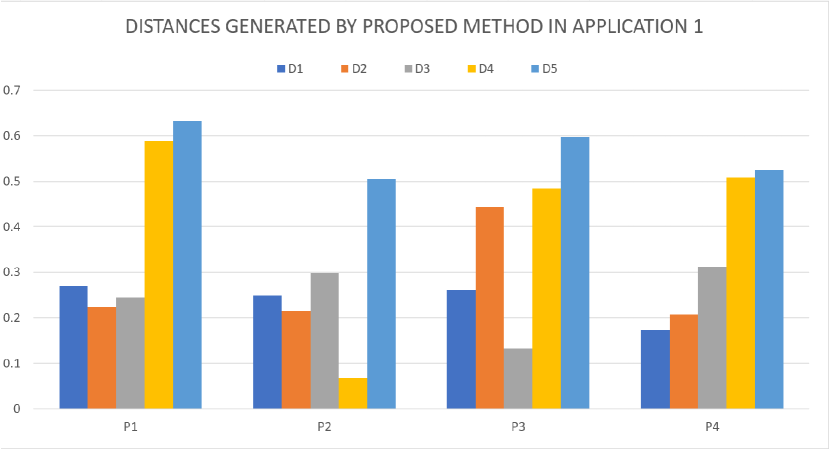
Figure 3:

TABLE XII: Distances generated by proposed method in application 2

$Patients$	$Distances$
	$D_{1}$	$D_{2}$	$D_{3}$	$D_{4}$	$D_{5}$
$P_{1}$	$0.5457$	$0.4593$	$0.5213$	$0.4847$	$0.6497$
$P_{2}$	$0.2224$	$0.5103$	$0.2680$	$0.3987$	$0.4768$
$P_{3}$	$0.6160$	$0.6561$	$0.5438$	$0.3955$	$0.6716$
$P_{4}$	$0.5058$	$0.4265$	$0.4444$	$0.4393$	$0.5723$

TABLE XIII: Judgements generated by different methods in application 2

$Methods$	$Diagnoses$
	$P_{1}$	$P_{2}$	$P_{3}$	$P_{4}$
Ngan et al. [72]	$Malaria$	$Stomach\ problem$	$Typhoid$	$Malaria$
Proposed method	$Malaria$	$Viral\ fever$	$Stomach\ problem$	$Malaria$

TABLE XIV: Symptoms expressed in the form of PFS of patients in application 3

$Patients$	$Symptom1$	$Symptom2$	$Symptom3$	$Symptom4$	$Symptom5$
$P_{1}$	$\langle a_{1},0.90,0.10\rangle$	$\langle a_{2},0.70,0.20\rangle$	$\langle a_{3},0.20,0.80\rangle$	$\langle a_{4},0.70,0.20\rangle$	$\langle a_{5},0.20,0.70\rangle$
$P_{2}$	$\langle a_{1},0.00,0.70\rangle$	$\langle a_{2},0.40,0.50\rangle$	$\langle a_{3},0.60,0.20\rangle$	$\langle a_{4},0.20,0.70\rangle$	$\langle a_{5},0.10,0.20\rangle$
$P_{3}$	$\langle a_{1},0.70,0.10\rangle$	$\langle a_{2},0.70,0.10\rangle$	$\langle a_{3},0.00,0.50\rangle$	$\langle a_{4},0.10,0.70\rangle$	$\langle a_{5},0.00,0.60\rangle$
$P_{4}$	$\langle a_{1},0.50,0.10\rangle$	$\langle a_{2},0.40,0.30\rangle$	$\langle a_{3},0.40,0.50\rangle$	$\langle a_{4},0.80,0.20\rangle$	$\langle a_{5},0.30,0.40\rangle$

TABLE XV: Symptoms expressed in the form of PFS of diagnoses in application 3

$Diagnoses$	$Symptom1$	$Symptom2$	$Symptom3$	$Symptom4$	$Symptom5$
$D_{1}$	$\langle a_{1},0.30,0.00\rangle$	$\langle a_{2},0.30,0.50\rangle$	$\langle a_{3},0.20,0.80\rangle$	$\langle a_{4},0.70,0.30\rangle$	$\langle a_{5},0.20,0.60\rangle$
$D_{2}$	$\langle a_{1},0.00,0.60\rangle$	$\langle a_{2},0.20,0.60\rangle$	$\langle a_{3},0.00,0.80\rangle$	$\langle a_{4},0.50,0.00\rangle$	$\langle a_{5},0.10,0.80\rangle$
$D_{3}$	$\langle a_{1},0.20,0.20\rangle$	$\langle a_{2},0.50,0.20\rangle$	$\langle a_{3},0.10,0.70\rangle$	$\langle a_{4},0.20,0.60\rangle$	$\langle a_{5},0.20,0.80\rangle$
$D_{4}$	$\langle a_{1},0.20,0.80\rangle$	$\langle a_{2},0.10,0.50\rangle$	$\langle a_{3},0.70,0.00\rangle$	$\langle a_{4},0.10,0.70\rangle$	$\langle a_{5},0.20,0.70\rangle$
$D_{5}$	$\langle a_{1},0.20,0.80\rangle$	$\langle a_{2},0.00,0.70\rangle$	$\langle a_{3},0.20,0.80\rangle$	$\langle a_{4},0.10,0.80\rangle$	$\langle a_{5},0.80,0.10\rangle$

TABLE XVI: Distances generated by proposed method in application 3

$Patients$	$Distances$
	$D_{1}$	$D_{2}$	$D_{3}$	$D_{4}$	$D_{5}$
$P_{1}$	$0.1930$	$0.3979$	$0.2707$	$0.6404$	$0.6942$
$P_{2}$	$0.4230$	$0.3648$	$0.2882$	$0.1181$	$0.3191$
$P_{3}$	$0.3558$	$0.4174$	$0.0996$	$0.4498$	$0.5463$
$P_{4}$	$0.1658$	$0.2727$	$0.3270$	$0.4664$	$0.5125$

TABLE XVII: Judgements generated by different methods in application 3

$Methods$	$Diagnoses$
	$P_{1}$	$P_{2}$	$P_{3}$	$P_{4}$
Smuel and Rajakumar [73]	$Stress$	$Spinal\ problem$	$Vision\ problem$	$Stress$
Xiao [74]	$Stress$	$Spinal\ problem$	$Vision\ problem$	$Stress$
Proposed method	$Stress$	$Spinal\ problem$	$Vision\ problem$	$Stress$

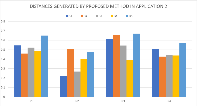
Figure 4:

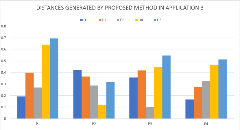
Figure 5:

Application 2 : Suppose there are four patients, namely $Ram$, $Mari$, $Sugu$ and $Somu$, who are denoted as $P=\{P_{1},P_{2},P_{3},P_{4}\}$. Besides, five attibutes which are symptoms in fact are introdeced as $Temperature$, $Headache$, $Stomach\ pain$, $Cough$ and $Chest\ pain$, which are denoted as $A=\{a_{1},a_{2},a_{3},a_{4},a_{5}\}$. More than that, diagnostic results are divided into five categories, $Viralfever$, $Malaria$, $Typhoid$, $Stomach\ problem$ and $Chest$, which are also denoted as $D=\{D_{1},D_{2},D_{3},D_{4},D_{5}\}$. With the help of the concept of PFS, all of the examples are presented in the form of PFS, which is effective in judging proper patterns. And every details of the patients are shown in table $10$. Additionaly, the diagnoses in the form of PFS are also presented in table $11$. By using the new proposed method of measuring distance betweent PFSs, all the results generated by the new proposed method are shown in table $12$. According the standards raised in the algorithm and other methods, all of final judgements are presented in table $13$.
Although the results produced by two methods are some kind of different, it can be easily inferred that the new proposed method conforms to the actual situation. With respect to patient $1$ and patient $4$, two methods have reached a agreement, which is satisfying. But when coming to judging patient $2$ and patient $3$, the situation is becoming more complex. The referenced method considers $Mari\ (P_{2})$ is suffering from $Stomach\ problem$, while the new proposed method illustrates that $Mari\ (P_{2})$ is diagnosed with $Viral\ fever$. Compared with the characteristics of patient $2$ and pattern $1$ and $4$, it can be concluded that the situation of patient $2$ conforms to every symptoms contained in pattern $1$ while the situation of patient $2$ is conflicting with pattern $4$ in symptoms $2$ and $3$, which indicates that there is a bigger probability of patient $1$ suffering from $Viral\ fever$ instead of $Stomach\ problem$. Similar circumstances occur in the judgment of patient $3$. The referenced method considers $Sugu\ (P_{3})$ is suffering from $Typhoid$, while the new proposed method illustrates that $Sugu\ (P_{3})$ is diagnosed with $Stomach\ problem$. Patient $3$ is conflicting with pattern $3$ in symptoms $1$ and $2$ while the situation of patient $3$ is only discordant with the symptom $1$, which indicates that the judgements given by the new proposed method are more rational and intuitive according to the data offered in table $10$ and $11$. As a result, the new proposed method has much better performance in handling actual cases.

Application 3 : Suppose there are four patients, namely $Ragu$, $Mathi$, $Velu$ and $Karthi$, who are denoted as $P=\{P_{1},P_{2},P_{3},P_{4}\}$. Besides, five attibutes which are symptoms in fact are introdeced as $Headache$, $Acidity$, $Burning\ eyes$, $Back\ pain$ and $Depression$, which are denoted as $A=\{a_{1},a_{2},a_{3},a_{4},a_{5}\}$. More than that, diagnostic results are divided into five categories, $Stress$, $Ulcer$, $Vision\ problem$, $Spinal\ problem$ and $Bloodpressure$, which are also denoted as $D=\{D_{1},D_{2},D_{3},D_{4},D_{5}\}$. With the help of the concept of PFS, all of the examples are presented in the form of PFS, which is effective in judging proper patterns. And every details of the patients are shown in table $14$. Additionaly, the diagnoses in the form of PFS are also presented in table $15$. By using the new proposed method of measuring distance betweent PFSs, all the results generated by the new proposed method are shown in table $16$. According the standards raised in the algorithm and other methods, all of final judgements are presented in table $17$.
After checking the results generated by the new propsoed methods, $P_{1}$ has the least value of $\widetilde{D}_{N}=0.1930$; $P_{2}$ has the least value of $\widetilde{D}_{N}=0.1181$; $P_{3}$ has the least value of $\widetilde{D}_{N}=0.0996$; $P_{4}$ has the least value of $\widetilde{D}_{N}=0.1658$. All in all, the results produced by Sumuel and Rajakumar’s method and Xiao’s method conform to the ones produced by the new proposed method, which proves that the accuracy and validity of the new proposed method in real application and the feasibility of the new proposed method in practical usage.

V Conclusion

In the theory of pythagorean fuzzy sets, how to accurately and properly measure the distance between PFSs is still an open issue, which may lead to chaos in pattern recognition. To solve this problem, in this paper, a completely new method of measuring distance between different PFSs is proposed, which statisfy all of the properties required by the axiom of measurement. The mainadvantage of the new proposed method is that it considers the indec of hesitance and distribute its mass to membership and non-membership in a reasonable way to strengthen the role which membership and non-membership plays in generating distances betweent PFSs. Besides, the rudction in the index of hesitance is also very important in alleviating the vagueness in PFSs and helpful in recognizing corresponding targets or patterns. Owing to this operation, the accuracy of the new proposed method is further improved. All in all, the proposeed method produces much more rational results than some previous methods, which is more closer to actual situations and conforms to intuitive judgements. When compared with other methods, the results produced by the proposed method also reached an agreement with the ones generated by other methods, which demonstrates the feasibility of the new proposed method in practical application. In this paper, the algorithm which is developed on the basis of the new proposed method offers a promising and reliable solution to address the recognition problems in medical diagnosis. And in future, this new proposed method can be used to measure vagueness, correlation and so on in corresponding research areas.

References

• [1] Y. Deng, “Uncertainty measure in evidence theory,” SCIENCE CHINA Information Sciences, vol. 64, pp. 10.1007/s11 432–020–3006–9, 2021.
• [2] F. Buono and M. Longobardi, “A dual measure of uncertainty: The deng extropy,” Entropy, vol. 22, no. 5, 2020. [Online]. Available: https://www.mdpi.com/1099-4300/22/5/582
• [3] X. Gao, F. Liu, L. Pan, Y. Deng, and S.-B. Tsai, “Uncertainty measure based on Tsallis entropy in evidence theory,” International Journal of Intelligent Systems, vol. 34, no. 11, pp. 3105–3120, 2019.
• [4] Y. Song, Q. Fu, Y.-F. Wang, and X. Wang, “Divergence-based cross entropy and uncertainty measures of Atanassov’s intuitionistic fuzzy sets with their application in decision making,” Applied Soft Computing, vol. 84, p. 105703, 2019.
• [5] P. Liu and X. Zhang, “A new hesitant fuzzy linguistic approach for multiple attribute decision making based on Dempster–Shafer evidence theory,” Applied Soft Computing, vol. 86, p. 105897, 2020.
• [6] A. P. Dempster, “Upper and Lower Probabilities Induced by a Multi-Valued Mapping,” Annals of Mathematical Statistics, vol. 38, no. 2, pp. 325–339, 1967.
• [7] L. A. Zadeh, “A Simple View of the Dempster-Shafer Theory of Evidence and Its Implication for the Rule of Combination,” Ai Magazine, vol. 7, no. 2, pp. 85–90, 1986.
• [8] R. R. Yager, “Generalized Dempster–Shafer structures,” IEEE Transactions on Fuzzy Systems, vol. 27, no. 3, pp. 428–435, 2019.
• [9] ——, “On the Dempster-Shafer framework and new combination rules,” Information sciences, vol. 41, no. 2, pp. 93–137, 1987.
• [10] Q. Zhou, H. Mo, and Y. Deng, “A new divergence measure of Pythagorean fuzzy sets based on belief function and its application in medical diagnosis,” Mathematics, vol. 8, no. 1, p. DOI: 10.3390/math8010142, 2020.
• [11] W. Jiang, “A correlation coefficient for belief functions,” International Journal of Approximate Reasoning, vol. 103, pp. 94–106, 2018.
• [12] F. Xiao, “A new divergence measure for belief functions in D-S evidence theory for multisensor data fusion,” Information Sciences, vol. 514, pp. 462–483, 2020.
• [13] L. Pan and Y. Deng, “An association coefficient of belief function and its application in target recognition system,” International Journal of Intelligent Systems, vol. 35, pp. 85–104, 2020.
• [14] E. Lefevre, O. Colot, and P. Vannoorenberghe, “Belief function combination and conflict management,” Information Fusion, vol. 3, no. 2, pp. 149 – 162, 2002. [Online]. Available: http://www.sciencedirect.com/science/article/pii/S1566253502000532
• [15] Y. Deng, W. Shi, Z. Zhu, and Q. Liu, “Combining belief functions based on distance of evidence,” Decision support systems, vol. 38, no. 3, pp. 489–493, 2004.
• [16] C. K. Murphy, “Combining belief functions when evidence conflicts,” Decision Support Systems, vol. 29, no. 1, pp. 1 – 9, 2000. [Online]. Available: http://www.sciencedirect.com/science/article/pii/S0167923699000846
• [17] Y. Xue and Y. Deng, “Entailment for Intuitionistic fuzzy sets based on generalized belief structures,” International Journal of Intelligent Systems, vol. 35, pp. 963–982, 2020.
• [18] R. R. Yager, “Entailment for measure based belief structures,” Information Fusion, vol. 47, pp. 111–116, 2019.
• [19] X. Deng and W. Jiang, “On the negation of a Dempster–Shafer belief structure based on maximum uncertainty allocation,” Information Sciences, vol. 516, pp. 346–352, 2020.
• [20] C. Fu, M. Xue, D.-L. Xu, and S.-L. Yang, “Selecting strategic partner for tax information systems based on weight learning with belief structures,” International Journal of Approximate Reasoning, vol. 105, pp. 66–84, 2019.
• [21] D. Li, X. Gao, and Y. Deng, “A Generalized Expression for Information Quality of Basic Probability Assignment,” IEEE Access, vol. 7, pp. 174 734–174 739, 2019.
• [22] M. Jing and Y. Tang, “A new base basic probability assignment approach for conflict data fusion in the evidence theory,” Applied Intelligence, pp. 1–13, 2020.
• [23] Z. Luo and Y. Deng, “A vector and geometry interpretation of basic probability assignment in Dempster-Shafer theory,” International Journal of Intelligent Systems, vol. 35, no. 6, pp. 944–962, 2020.
• [24] J. Zhang, R. Liu, J. Zhang, and B. Kang, “Extension of Yager’s negation of a probability distribution based on Tsallis entropy,” International Journal of Intelligent Systems, vol. 35, no. 1, pp. 72–84, 2020.
• [25] R. R. Yager, “On the maximum entropy negation of a probability distribution,” IEEE Transactions on Fuzzy Systems, vol. 23, no. 5, pp. 1899–1902, 2014.
• [26] L. Pan and Y. Deng, “Probability transform based on the ordered weighted averaging and entropy difference,” International Journal of Computers Communications & Control, vol. 15, no. 4, p. 3743, 2020.
• [27] F. Xiao, “A multiple-criteria decision-making method based on D numbers and belief entropy,” International Journal of Fuzzy Systems, vol. 21, no. 4, pp. 1144–1153, 2019.
• [28] S. Duan, T. Wen, and W. Jiang, “A new information dimension of complex network based on Rényi entropy,” Physica A: Statistical Mechanics and its Applications, vol. 516, pp. 529–542, 2019.
• [29] H. Yan and Y. Deng, “An improved belief entropy in evidence theory,” IEEE Access, vol. 8, no. 1, pp. 57 505–57 516, 2020.
• [30] J. Abellán, “Analyzing properties of Deng entropy in the theory of evidence,” Chaos, Solitons & Fractals, vol. 95, pp. 195–199, 2017.
• [31] Y. Deng, “Deng entropy,” Chaos, Solitons & Fractals, vol. 91, pp. 549–553, 2016.
• [32] Z. Cao, W. Ding, Y.-K. Wang, F. K. Hussain, A. Al-Jumaily, and C.-T. Lin, “Effects of Repetitive SSVEPs on EEG Complexity using Multiscale Inherent Fuzzy Entropy,” Neurocomputing, p. DOI: 10.1016/j.neucom.2018.08.091, 2019.
• [33] F. Xiao, “Multi-sensor data fusion based on the belief divergence measure of evidences and the belief entropy,” Information Fusion, vol. 46, pp. 23–32, 2019.
• [34] B. Kang, P. Zhang, Z. Gao, G. Chhipi-Shrestha, K. Hewage, and R. Sadiq, “Environmental assessment under uncertainty using Dempster–Shafer theory and Z-numbers,” Journal of Ambient Intelligence and Humanized Computing, pp. DOI: 10.1007/s12 652–019–01 228–y, 2019.
• [35] Y. Li, H. Garg, and Y. Deng, “A New Uncertainty Measure of Discrete Z-numbers,” International Journal of Fuzzy Systems, vol. 22, no. 3, pp. 760–776, 2020.
• [36] W. Jiang, Y. Cao, and X. Deng, “A novel Z-network model based on Bayesian network and Z-number,” IEEE Transactions on Fuzzy Systems, p. DOI: 10.1109/TFUZZ.2019.2918999, 2019.
• [37] L. A. Zadeh, “A note on Z-numbers,” Information Sciences, vol. 181, no. 14, pp. 2923–2932, 2011.
• [38] Q. Liu, Y. Tian, and B. Kang, “Derive knowledge of Z-number from the perspective of Dempster–Shafer evidence theory,” Engineering Applications of Artificial Intelligence, vol. 85, pp. 754–764, 2019.
• [39] B. liu and Y. Deng, “Risk evaluation in failure mode and effects analysis based on D numbers theory,” International Journal of Computers Communications & Control, vol. 14, no. 5, pp. 672–691, 2019.
• [40] X. Deng, Y. Hu, Y. Deng, and S. Mahadevan, “Environmental impact assessment based on D numbers,” Expert Systems with Applications, vol. 41, no. 2, pp. 635–643, 2014.
• [41] Y. Deng, “D numbers: theory and applications,” Journal of Information &Computational Science, vol. 9, no. 9, pp. 2421–2428, 2012.
• [42] F. Xiao, “A multiple-criteria decision-making method based on D numbers and belief entropy,” International Journal of Fuzzy Systems, vol. 21, no. 4, pp. 1144–1153, 2019.
• [43] X. Deng and W. Jiang, “A total uncertainty measure for D numbers based on belief intervals,” International Journal of Intelligent Systems, vol. 34, no. 12, pp. 3302–3316, 2019.
• [44] L. A. Zadeh, “Fuzzy sets,” Information and control, vol. 8, no. 3, pp. 338–353, 1965.
• [45] ——, “Fuzzy sets and information granularity,” Advances in fuzzy set theory and applications, vol. 11, pp. 3–18, 1979.
• [46] F. Xiao, “A distance measure for intuitionistic fuzzy sets and its application to pattern classification problems,” IEEE Transactions on Systems, Man, and Cybernetics: Systems, pp. 1–13, 2019.
• [47] Z. Liu, Y. Liu, J. Dezert, and F. Cuzzolin, “Evidence combination based on credal belief redistribution for pattern classification,” IEEE Transactions on Fuzzy Systems, p. DOI: 10.1109/TFUZZ.2019.2911915, 2019.
• [48] Y. Song, X. Wang, W. Wu, W. Quan, and W. Huang, “Evidence combination based on credibility and non-specificity,” Pattern Analysis and Applications, vol. 21, no. 1, pp. 167–180, 2018.
• [49] Y. Deng, X. Su, D. Wang, and Q. Li, “Target recognition based on fuzzy dempster data fusion method,” Defence Science Journal, vol. 60, no. 5, 2010.
• [50] R. R. Yager, “Weighted maximum entropy owa aggregation with applications to decision making under risk,” IEEE Transactions on Systems, Man, and Cybernetics-Part A: Systems and Humans, vol. 39, no. 3, pp. 555–564, 2009.
• [51] Y. Han, Y. Deng, Z. Cao, and C.-T. Lin, “An interval-valued Pythagorean prioritized operator based game theoretical framework with its applications in multicriteria group decision making,” Neural Computing and Applications, pp. DOI: 10.1007/s00 521–019–04 014–1, 2019.
• [52] L. Fei, J. Xia, Y. Feng, and L. Liu, “An ELECTRE-based multiple criteria decision making method for supplier selection using Dempster-Shafer theory,” IEEE Access, vol. 7, pp. 84 701–84 716, 2019.
• [53] R. R. Yager, “Weighted maximum entropy owa aggregation with applications to decision making under risk,” IEEE Transactions on Systems, Man, and Cybernetics-Part A: Systems and Humans, vol. 39, no. 3, pp. 555–564, 2009.
• [54] K. T. Atanassov, “Intuitionistic fuzzy sets.”   Springer, 1999, pp. 1–137.
• [55] C.-P. Wei, P. Wang, and Y.-Z. Zhang, “Entropy, similarity measure of interval-valued intuitionistic fuzzy sets and their applications,” Information Sciences, vol. 181, no. 19, pp. 4273 – 4286, 2011. [Online]. Available: http://www.sciencedirect.com/science/article/pii/S0020025511002751
• [56] K. T. Atanassov, Interval-Valued Intuitionistic Fuzzy Sets, ser. Studies in Fuzziness and Soft Computing.   Springer, 2020, vol. 388. [Online]. Available: https://doi.org/10.1007/978-3-030-32090-4
• [57] W. Ding, C. Lin, M. Prasad, Z. Cao, and J. Wang, “A layered-coevolution-based attribute-boosted reduction using adaptive quantum-behavior pso and its consistent segmentation for neonates brain tissue,” IEEE Transactions on Fuzzy Systems, vol. 26, no. 3, pp. 1177–1191, 2018.
• [58] R. R. Yager, “Pythagorean fuzzy subsets,” in 2013 Joint IFSA World Congress and NAFIPS Annual Meeting (IFSA/NAFIPS), 2013, pp. 57–61.
• [59] R. Yager and A. Abbasov, “Pythagorean Membership Grades, Complex Numbers, and Decision Making,” International Journal of Intelligent Systems, vol. 28, pp. 436–452, 2013.
• [60] R. Yager, “Pythagorean Membership Grades in Multicriteria Decision Making,” IEEE Transactions on Fuzzy Systems, vol. 22, pp. 958–965, 2014.
• [61] L. Fei and Y. Deng, “Multi-criteria decision making in Pythagorean fuzzy environment,” Applied Intelligence, vol. 50, no. 2, pp. 537–561, 2020.
• [62] R. R. Yager, “Properties and applications of Pythagorean fuzzy sets,” in Imprecision and Uncertainty in Information Representation and Processing.   Springer, 2016, pp. 119–136.
• [63] E. Szmidt and J. Kacprzyk, “Distances between intuitionistic fuzzy sets,” Fuzzy Sets and Systems, vol. 114, no. 3, pp. 505 – 518, 2000. [Online]. Available: http://www.sciencedirect.com/science/article/pii/S0165011498002449
• [64] P. Grzegorzewski, “Distances between intuitionistic fuzzy sets and/or interval-valued fuzzy sets based on the hausdorff metric,” Fuzzy Sets and Systems, vol. 148, no. 2, pp. 319 – 328, 2004. [Online]. Available: http://www.sciencedirect.com/science/article/pii/S0165011403003543
• [65] c.-m. Own, “Switching between type-2 fuzzy sets and intuitionistic fuzzy sets: An application in medical diagnosis,” Appl. Intell., vol. 31, pp. 283–291, 12 2009.
• [66] S. K. De, R. Biswas, and A. R. Roy, “An application of intuitionistic fuzzy sets in medical diagnosis,” Fuzzy Sets and Systems, vol. 117, no. 2, pp. 209 – 213, 2001. [Online]. Available: http://www.sciencedirect.com/science/article/pii/S0165011498002358
• [67] E. Szmidt and J. Kacprzyk, “Intuitionistic fuzzy sets in intelligent data analysis for medical diagnosis,” in Computational Science - ICCS 2001, V. N. Alexandrov, J. J. Dongarra, B. A. Juliano, R. S. Renner, and C. J. K. Tan, Eds.   Berlin, Heidelberg: Springer Berlin Heidelberg, 2001, pp. 263–271.
• [68] S. Pramanik and K. Mondal, “Intuitionistic fuzzy similarity measure based on tangent function and its application to multi-attribute decision making,” Global Journal of Advanced Research, vol. 2, pp. 464–471, 02 2015.
• [69] T.-Y. Chen, “Remoteness index-based pythagorean fuzzy vikor methods with a generalized distance measure for multiple criteria decision analysis,” Information Fusion, vol. 41, pp. 129 – 150, 2018. [Online]. Available: http://www.sciencedirect.com/science/article/pii/S1566253517300763
• [70] S.-M. Chen and J.-M. Tan, “Handling multicriteria fuzzy decision-making problems based on vague set theory,” Fuzzy Sets and Systems, vol. 67, pp. 163–172, 10 1994.
• [71] C. Cheng, F. Xiao, and Z. Cao, “A new distance for intuitionistic fuzzy sets based on similarity matrix,” IEEE Access, vol. 7, pp. 70 436–70 446, 2019.
• [72] R. Ngan, M. Ali, and L. Son, “-equality of intuitionistic fuzzy sets: a new proximity measure and applications in medical diagnosis,” Applied Intelligence, vol. 48, 02 2018.
• [73] X. Deng, “Analyzing the monotonicity of belief interval based uncertainty measures in belief function theory,” International Journal of Intelligent Systems, vol. 33, 03 2018.
• [74] F. Xiao, “Divergence measure of pythagorean fuzzy sets and its application in medical diagnosis,” Applied Soft Computing, vol. 79, 04 2019.