Study of Gravastars in Rastall Gravity

Abstract

Gravastars have been considered as a feasible alternative to black holes in the past couple of decades. Stable models of gravastar have been studied in many of the alternative gravity theories besides standard General Relativity (GR). The Rastall theory of gravity is a popular alternative to GR, specially in the cosmological and astrophysical context. Here, we propose a stellar model under the Rastall gravity following Mazur-Mottola’s [1, 2] conjecture. The gravastar consists of three regions, viz., ($I$) Interior region, ($II$) Intermediate shell region, and ($III$) Exterior region. The pressure within the interior core region is assumed with a constant negative matter-energy density which provides a repulsive force over the entire thin shell region. The shell is assumed to be made up of fluid of ultrarelativistic plasma which follows the Zel’dovich’s conjecture of stiff fluid [3, 4]. It is also assumed that the pressure is proportional to the matter-energy density according to Zel’dovich’s conjecture, which cancel the repulsive force exerted by the interior region. The exterior region is completely vacuum which is described by the Schwarzschild-de Sitter solution. Under all these specifications we obtain a set of exact and singularity-free solutions of the gravastar model presenting several physically valid features within the framework of Rastall gravity. The physical properties of the shell region namely, the energy density, proper length, total energy and entropy are explored. The stability of the gravastar model is investigated using the surface redshift against the shell thickness and maximizing the entropy of the shell within the framework of Rastall gravity.

1 Introduction

The end point of the stellar evolution of a massive object always attract the attention of the astrophysicists. It is conjectured that in the final stage of stellar evolution if the mass of the stellar remnant after forming planetary nebula or initiating supernova explosion is greater than three solar mass, then the collapsing phase of the star due its self gravitational pull leads to a highly dense object, i.e., black hole. In 1916, Schwarzschild obtained the simplest black hole solution from the Einstein field equation in vacuum which is considered as the important solution of a classical black hole (static as well as uncharged). But the Schwarzschild solution has some shortcomings due to (i) presence of singularity inside the black hole, (ii) existence of event horizon which leads to major unsolved issues. Mazur and Mottola [1, 2] first proposed a new idea of collapsing stellar object by considering an extended idea of Bose Einstein Condensation (BEC) in the gravitating system. In the model it was proposed that one can construct a cold, dark and compact object, they nomenclature it as a Gravitational Vacuum Condensed Star or Gravastar. The model of gravastar satisfies all the theoretical criterion for a stable end point of the stellar evolution and provides solution to the problems of classical black hole. After the successful detection of gravitation wave (GW) in 2015 [5], it is assumed that the GWs are originated due to merging of two massive black holes. As the observational signals does not confirm the recovery of the basic problems of black holes, it demands an alternative approach to describe the shortcomings. In this context, the gravastar may play an important role to describe the final state of the stellar evolution. Though there are no sufficient observational evidences in favour of gravastars directly for their existence, it is important to study the concept of gravastar that can be claimed as a viable alternative to resolve the conceptual issues in understanding the black holes.

The gravastar consists of three regions namely interior region, intermediate thin shell, and exterior region. As proposed by Mazur and Mottola [1, 2] the interior region of the gravastar being in de Sitter condensate phase is assumed to be filled with vacuum energy, the exterior region is completely vacuum known as Schwarzschild vacuum, and those two regions are separated by a thin shell of ultra-relativistic matter of very high density. The barotropic equation of state (EOS) is $p=\omega\rho$, where $p$ and $\rho$ are the pressure and matter-energy density respectively and $\omega$ is the EOS parameter.

In a gravastar the EOS parameter $\omega$, is different in different regions as follows:
($I$) Interior Region : $0\leq r<R_{1}$, $\omega=-1$, $i.e.$, EOS is $p=-\rho$ ,
($II$) Thin Shell Region: $R_{1}<r<R_{2}$, $\omega=1$, $i.e.$, EOS is $p=\rho$ ,
($III$) Exterior Region : $R_{2}<r$, $\omega=0$, $i.e.$, EOS is $p=\rho=0$ .
where $R_{1}$ and $R_{2}$ represent the radii of the interior and exterior boundary of the gravastar respectively. Therefore, thickness of the intermediate shell region is given by $R_{2}-R_{1}=\epsilon\ (say)$, where $\epsilon\ll 1$ because in a gravastar the thickness of the shell is very small compared to its size.

The idea of gravastar is discussed in the literature [6, 7, 8, 9, 10, 11, 12, 13, 14, 15, 16, 17, 19, 18, 20, 21, 22, 23, 24, 25, 26, 27, 28, 29, 30, 31] as an alternative to BH. Mazur and Mottola proposed a three layer structure of the gravastar and studied the thermodynamical stability employing the entropy maximization technique, whereas Visser [6] showed the dynamical stability of the system. Based on the three layer system it is now established that the theoretical acceptance of gravastar model in both lower and higher dimensions with or without charge is important in astrophysics. Usmani et al. [17] shown the possibility of existence of higher dimensional gravastar, and later on Bhar [24] and Ghosh et al. [26] studied the higher dimensional gravastar with and without conformal motion respectively. The possibility of gravastar in lower dimension is also studied [28, 29]. Chan and Silva [30] have investigated the effect of charge on the stability of the gravastar formation considering a charged shell configuration. Again, considering the Vaidya exterior spacetime, Chan $et~{}al.$ [31] have studied the dynamical models of prototype radiating gravastars and showed that the final output may corresponds to a number of objects, a black hole, an unstable gravastar, a stable gravastar or a “bounded excursion” gravastar depending on the mass of the shell that evolves in time, the cosmological constant, and the initial position of the dynamical shell. All of these works are mainly carried out in the framework of Einstein’s general theory of relativity (GR). Though it is well known that Einstein’s GR is one of the most promising theory for revealing most of the hidden mysteries of the Nature it is realized that a modification of the GR is inevitable to wipe out shortcomings in the theoretical as well as observational aspects. The confirmation of accelerated universe based on some observational evidences as well as the existence of dark matter and dark energy led to a theoretical challenge to GR  [32, 33, 34, 35, 36, 37, 38, 39, 40, 41, 42]. To accommodate the present acceleration of the universe a number of alternative theories of gravity, namely $f(R)$ gravity, $f(\mathbb{T})$ gravity, $f(R,\mathcal{T})$ gravity, $f(\mathbb{T},\mathcal{T})$ gravity are developed successively with a modification either in the geometrical part or in the matter-energy part of Einstein field equations. In most of these theories different functions of the Ricci scalar with or without other scalar quantities are incorporated in the gravitational Lagrangian of the corresponding Einstein-Hilbert action. A lot of works have been performed on compact stars as well as gravastars under the framework of modified theories of gravity as available in the literature [43, 44, 45, 46, 47, 48, 49, 50]. But, in most these theories the energy-momentum tensor (EMT) is not generally conserved unlike the case of general relativity. This interesting aspect of modified gravity motivates us to make a general study of gravastar under the Rastall theory of gravity as proposed by Rastall in 1972 [51, 52] based on the idea that the usual law of conservation of energy-momentum tensor, i.e., $\nabla_{\nu}T_{\mu}^{\nu}=0$ is violated when a curved spacetime is taken into account. The violation of conservation law of EMT is the key point of this modification where the covariant derivative of EMT is directly proportional to the divergence of scalar curvature. Mathematically, it can be written as $\nabla_{\nu}T_{\mu}^{\nu}\propto\mathcal{R}_{,\;\mu}$, which further takes the form $\nabla_{\nu}T_{\mu}^{\nu}=\psi\mathcal{R}_{,\;\mu}$, where $\psi$ is the constant of proportionality.

Various cosmological as well as astrophysical aspects have been investigated under the framework of Rastall theory due its numerous appealing features and simpler form of field equations as available in the literatures [53, 54, 55, 56, 57, 58, 59, 60, 61, 62]. Recently, in astrophysical context Rastall gravity has been extensively investigated in the context of rotating black holes [58], Kerr-Newman-AdS black hole [59], non commutative geometry [60]. Rastall theory is also successful in the context of relativistic solutions of compact stars. Oliveira $et~{}al.$ [61] have studied Neutron stars in Rastall gravity. Bhar et al. [62] studied a highly dense compact object in Rastall gravity using Tolman-Kuchowicz spacetime.

The outline of the present investigation is as follows: In section 2 the basic mathematical formalism of Rastall theory is presented and the explicit form of the field equations along with the conservation equation of Rastall gravity is given, in section 3, we obtain the solutions of the field equations considering the different regions, viz., interior region, exterior region, and shell region of the gravastar. In section 4, we consider the matching conditions in order to determine the numerical values of several constants which arise in different calculations. Section 5 deals with some physical features of the model, i.e., proper length, pressure, energy, and entropy within the shell region. Junction conditions are presented in section 6. Stability issue of the model has been explored in section 7, and finally, we pass some concluding remarks in section 8.

2 The Field Equations geometry in Rastall theory

We start from the short introduction to Rastall theory of gravity which was introduced by P. Rastall [51, 52]. According to the original idea of Rastall [51], the vanishing of covariant divergence of the matter energy-momentum tensor is no longer valid and this vector field is proportional to the covariant derivative of the Ricci curvature scalar as,

$$\nabla_{\nu}T_{\mu}^{\nu}=a_{\mu}$$ (2.1)

where the functions $a_{\mu}$ vanish in flat space-time, but not in curved space-time, and which are in agreement with present observations. Here, it is noted that $a_{\mu}=\psi\mathcal{R}_{,\;\mu}$, where $\psi$ is a constant, $\mathcal{R}=g^{\mu\nu}\mathcal{R}_{\mu\nu}=g^{\mu\nu}g^{\lambda\pi}\mathcal{R}_{\lambda\mu\nu\pi}$ is the curvature invariant, $\mathcal{R}$ and $T_{\mu}^{\nu}$ represent the Ricci scalar and energy momentum tensor respectively and the comma denotes the partial derivative. The primary mathematical relation of Rastall gravity in terms of energy-momentum tensor and curvature scalar is defined by,

$$\mathcal{R}_{\mu\nu}+(k\psi-\frac{1}{2})g_{\mu\nu}\mathcal{R}=kT_{\mu\nu}$$ (2.2)

The Eq. (2.2) leads to a modified theory whose field equations can be written as

$$\mathcal{G}_{\mu\nu}+k\;\psi g_{\mu\nu}\mathcal{R}=kT_{\mu\nu}$$ (2.3)

where $\mathcal{G}_{\mu\nu}$ represents Einstein tensor. In the above set of field equations, the parameter $k$ plays the role of gravitational coupling parameter for modified Rastall theory. Contracting Eq. (2.2) one obtains $\mathcal{R}(4k\psi-1)=kT^{\mu}_{\;\mu}$. We exclude the case $k\psi=\frac{1}{4}$, since it implies that $T^{\mu}_{\;\mu}=0$, which is not always true. In empty space-time one has $T_{\mu\nu}=0$, and hence $\mathcal{R}=0$. The field equations then reduce to $\mathcal{R}_{\mu\nu}=0$, just as in the Einstein theory. In this study, we define $\xi=k\psi$ as the Rastall parameter, which can be considered as dimensionless. Consequently, the gravitational coupling parameter $k$ and the constant $\psi$ must satisfy:

$$k=\frac{8\pi G}{c^{4}}\left(\frac{4\xi-1}{6\xi-1}\right)$$ (2.4)

where $G$ is the Newtonian gravitational constant, and $c$ is the speed of light. When $\xi=0$, $k$ becomes the Einstein gravitational constant ($k=\frac{8\pi G}{c^{4}}$). It is also noted that $\xi=\frac{1}{4}$ is not permitted here. Thus, a new set of field equations for Rastall theory is given by

$$\mathcal{G}_{\mu\nu}+\xi\;g_{\mu\nu}\mathcal{R}=8\pi T_{\mu\nu}\left[\frac{4\xi-1}{6\xi-1}\right],$$ (2.5)

To study the gravastar in $(3+1)$ dimension we first consider the line element for the interior spacetime of a static spherically symmetric matter distribution is in the form

$$ds^{2}=-e^{\nu(r)}dt^{2}+e^{\mu(r)}dr^{2}+r^{2}(d\theta^{2}+sin^{2}\theta d\phi^{2}),$$ (2.6)

where $\mu$ and $\nu$ are the metric potentials which are function of r only.

Now we assume that the matter distribution in the interior of the star is that of a perfect fluid type and can be given by

$$T_{\mu\nu}=(\rho+p)u_{\mu}u_{\nu}+pg_{\mu\nu},$$ (2.7)

where $\rho$ represents energy density, $p$ is the isotropic pressure and $u^{\mu}$ represents four-velocity of the fluid under consideration such that $u^{\mu}=e^{-\nu/2}\delta^{\mu}_{0}$ with $u_{\mu}u^{\mu}=-1$.

Thus in Rastall gravity Eq. (2.5) along with Eq. (2.6) and Eq. (2.7) yields the following set of equations:

$$\frac{\left(4\xi-1\right)\rho(r)}{6\xi-1}=e^{-\mu}\left[\frac{\mu^{\prime}}{r}-\frac{1}{r^{2}}\right]+\frac{1}{r^{2}}+\xi e^{-\mu}\left[\nu^{\prime\prime}+(\nu^{\prime})^{2}-\mu^{\prime}\nu^{\prime}-\frac{2}{r}(\mu^{\prime}-\nu^{\prime})-\frac{2\left(e^{\mu}-1\right)}{r^{2}}\right],$$ (2.8)

$$\frac{(4\xi-1)p(r)}{6\xi-1}=e^{-\mu}\left[\frac{\nu^{\prime}}{r}+\frac{1}{r^{2}}\right]-\frac{1}{r^{2}}-e^{-\mu}\xi\left[\nu^{\prime\prime}+(\nu^{\prime})^{2}-\mu^{\prime}\nu^{\prime}-\frac{2}{r}(\mu^{\prime}-\nu^{\prime})-\frac{2\left(e^{\mu}-1\right)}{r^{2}}\right],$$ (2.9)

$$\frac{(4\xi-1)p(r)}{6\xi-1}=\frac{e^{-\mu}}{4}\left[2\nu^{\prime\prime}+\left(\nu^{\prime}\right)^{2}+\frac{2\nu^{\prime}}{r}-\frac{2\mu^{\prime}}{r}-\mu^{\prime}\nu^{\prime}\right]$$

$$-e^{-\mu}\xi\left[\nu^{\prime\prime}+(\nu^{\prime})^{2}-\mu^{\prime}\nu^{\prime}-\frac{2}{r}(\mu^{\prime}-\nu^{\prime})-\frac{2\left(e^{\mu}-1\right)}{r^{2}}\right].$$ (2.10)

Here the symbol ‘$\prime$’ denotes differentiation with respect to the radial parameter $r$ and the geometrized units $G=c=1$.

Therefore, the energy conservation equation in Rastall gravity can be written as

$$p^{\prime}+\frac{1}{2}(p+\rho)\nu^{\prime}-\frac{\xi}{{4\xi-1}}\left(\rho^{\prime}-3p^{\prime}\right)=0.$$ (2.11)

The above equation is different from that obtained in GR and can be retrieved in the limit $\xi\rightarrow 0$.

3 The gravastar models

Now we will study the three regions of gravastar precisely in Rastall theory of gravity.

3.1 Interior spacetime

According to Mazur-Mottola [1, 2], the interior region of gravastar can be described by the EOS as

$$p=-\rho$$ (3.1)

This negative (repulsive) pressure acting radially outward from the centre of the spherically symmetric gravitating system to counter balance the inward gravitational pull of the shell. The above EOS is known in the literature as a ‘degenerate vacuum’or‘$\rho$-vacuum’ [63, 64, 65, 66] which is a gravitational BEC after the phase transition occurring at the horizon (replaced by a shell for a gravastar) and it acts along the radially outward direction to oppose the collapse to be continued. Plugging this EOS in the conservation equation as provided by Eq. (3.1), we get that

$$p=-\rho=-\rho_{c}.$$ (3.2)

Here $\rho_{c}$ is the constant interior density, thus implying constant pressure.

Using Eq. (3.2) in the field Eqs. (2.8) and (2.9), we get the expression of the metric potential $\mu$ given by

$$\rm e^{-\mu(r)}=\frac{1}{3}C_{1}r^{2}-\frac{C^{\prime}}{3r}+1.$$ (3.3)

where $C_{1}$ and $C^{\prime}$ are integration constants. To make the solution regular at $r=0$ one can demand that $C^{\prime}=0$. Thus, Eq. (3.3) essentially reduces to

$$\rm e^{-\mu(r)}=\frac{1}{3}C_{1}r^{2}+1.$$ (3.4)

Again, from Eqs. (2.9) and (2.10) in the interior the another metric potential can be obtained as,

$$\rm e^{-\nu(r)}=C_{2}\left(\frac{1}{3}C_{1}r^{2}+1\right).$$ (3.5)

Here $C_{2}$ is an constant of integration. From the above solutions it can be noticed that the interior solutions have no singularity and thus the problem of the central singularity of a classical black hole can be averted.

The active gravitational mass of the interior region can be found by using the following equation as

$$\tilde{M}=\int^{R_{1}=R}_{0}4\pi r^{2}\rho dr=\frac{4\pi R^{3}\rho_{c}}{3}.$$ (3.6)

3.2 Intermediate thin shell

The shell consists of ultra relativistic fluid and it obeys the EOS $p=\rho$. In connection to cold baryonic universe, Zel’dovich [3, 4] first conceived the idea of this kind of fluid and it is also known as the stiff fluid. In the present case we can argue that this may arise from the thermal excitations with negligible chemical potential or from conserved number density of the gravitational quanta at the zero temperature. Several authors have extensively exploited this type of fluid to explore various cosmological [67, 68, 69] as well as astrophysical phenomena [72, 71, 70]. Within the non-vacuum region, i.e., the shell one can observe that it is very difficult to find solution of the field equations. However, within the framework of the thin shell limit, i.e., $0<e^{-\mu(r)}\ll 1$, it is possible to find an analytical solution. As prescribed by Israel we can possibly argue that the intermediate region between the two spacetimes must be a thin shell. Also within the thin shell region any parameter which is a function of r is, in general, $\ll 1$ as $r\rightarrow 0$. Due to this kind of approximation along with the above EOS as well as Eqs. (2.8), (2.9) and (2.10), one can obtain the following equations:

$$\frac{(4\xi-1)\rho(r)}{(6\xi-1)}={\frac{{e^{-\mu}}\mu^{\prime}}{r}}+\frac{1}{r^{2}}+{e^{-\mu}}\xi\left(-\mu^{\prime}\nu^{\prime}-\frac{2\mu^{\prime}}{r}\right)-\frac{2\xi}{r^{2}},$$ (3.7)

$$\frac{(4\xi-1)p(r)}{(6\xi-1)}=-\frac{1}{r^{2}}-{e^{-\mu}}\xi\left(-\mu^{\prime}\nu^{\prime}-\frac{2\mu^{\prime}}{r}\right)+\frac{2\xi}{r^{2}},$$ (3.8)

$$\frac{(4\xi-1)p(r)}{(6\xi-1)}=\frac{e^{-\mu}}{4}\left(-\mu^{\prime}\nu^{\prime}-\frac{2\mu^{\prime}}{r}\right)-{e^{-\mu}}\xi\left(-\mu^{\prime}\nu^{\prime}-{\frac{2\mu^{\prime}}{r}}\right)+\frac{2\xi}{r^{2}}.$$ (3.9)

From Eqs. (3.8)-(3.9) we get

$$\nu^{\prime}=\frac{-2e^{-\mu}\mu^{\prime}r+4}{e^{-\mu}r^{2}{\mu^{\prime}}}.$$ (3.10)

Now using Eqs. (3.7) and (3.8) along with the above condition we have obtained the two metric functions of the shell as follows,

$$e^{-\mu(r)}=-12\xi\ln(r)+2\ln(r)+C_{3},$$ (3.11)

$$\nu=\frac{4}{(6\xi-1)}\ln(r)-\frac{12\xi}{(6\xi-1)}\ln(r)+C_{4}.$$ (3.12)

where $C_{3}$ and $C_{4}$ are another two integration constants.

3.3 Exterior spacetime

The exterior of the gravastar is assumed to obey the EOS $p=\rho=0$ which means that the outside region of the shell is completely vacuum. Thus, using Eqs. (2.8) and (2.9), we get

$$\mu^{\prime}+\nu^{\prime}=0$$ (3.13)

Considering the solution of Eq. (3.13), one can consider the line element for the exterior region as the well-known Schwarzschild de Sitter metric which is given by

$$ds^{2}=-\left(1-\frac{2M}{r}-\frac{\Lambda r^{2}}{3}\right)dt^{2}+\left(1-\frac{2M}{r}-\frac{\Lambda r^{2}}{3}\right)^{-1}dr^{2}+r^{2}(d\theta^{2}+\sin^{2}\theta d\phi^{2}),$$ (3.14)

where $M$ is the total mass and $\Lambda$ is the cosmological constant.

4 Boundary Condition

The gravastar configuration has two boundaries, one is between interior region and intermediate thin shell (i.e., at $r=R_{1}$) and the other is between the shell and exterior spacetime (i.e., at $r=R_{2}$). For any stable configuration the metric functions must be continuous at these interfaces. In order to determine the unknown constants of our present study viz. $C_{1}$, $C_{2}$, $C_{3}$, $C_{4}$ and $\Lambda$, we have matched the metric functions at these boundaries and eventually obtained the values of these constants:

(i) At the boundary between the interior and the intermediate thin shell, $i.e.$ at $R=R_{1}$,

$$\frac{1}{3}C_{1}R_{1}^{2}+1=C_{3}-12\xi\log\left(R_{1}\right)+2\log\left(R_{1}\right),$$ (4.1)

$$C_{2}\left(\frac{1}{3}C_{1}R_{1}^{2}+1\right)=C_{4}R_{1}^{\frac{4-12\xi}{6\xi-1}}.$$ (4.2)

(ii) Again, from the continuity of the metric potentials and $\frac{\delta g_{tt}}{dr}$ at $R=R_{2}$ we get another three conditions

$$-\frac{2M}{R_{2}}-\frac{1}{3}\Lambda R_{2}^{2}+1=C_{3}-12\xi\log\left(R_{2}\right)+2\log\left(R_{2}\right),$$ (4.3)

$$-\frac{2M}{R_{2}}-\frac{1}{3}\Lambda R_{2}^{2}+1=C_{4}R_{2}^{\frac{4-12\xi}{6\xi-1}},$$ (4.4)

$$\frac{2M}{R_{2}^{2}}-\frac{2\Lambda R_{2}}{3}=\frac{C_{4}(4-12\xi)R_{2}^{\frac{4-12\xi}{6\xi-1}-1}}{6\xi-1}.$$ (4.5)

To obtain the numerical values of five different constants, i.e., $C_{1}$, $C_{2}$, $C_{3}$, $C_{4}$ and $\Lambda$ we choose the mass of the gravastar $M=3.75M_{\odot}$, interior radius $R_{1}=10$ km and the four different values of $\xi=0.228,0.23,0.235$ and $0.24$ which are enlisted in Table-I. We have also shown the predicted values of $R_{2}$ for different $\xi$ values from the concept of the surface energy density ($\Sigma$) (from section 6) in Table-I. In the present work we have made choice of the values for different parameters to study the physical behaviour for a stable stellar model of gravastar. Again, we also find different constants for a particular choice of $\xi=0.24$ by varying the mass value of gravastar as shown in Table-II. For a given combination of $M$ and $R_{2}$ it would provide an unique solution, but we have chosen the values to satisfy the ratio $\frac{2M}{r}<\frac{8}{9}$ and $Z_{s}<2$ for a stable model. As long as this relation holds good we can choose the set of $M$ and $R_{2}$ which provide similar behaviour as obtained in the paper.

$\xi$	$\Lambda$	$C_{1}$	$C_{2}$	$C_{3}$	$C_{4}$	Predicted $R_{2}$ (km.)
0.228	0.002902	-0.02501	0.9550	1.8607	0.00005636	10.055
0.23	0.002268	-0.02436	0.9589	1.9378	0.00009521	10.061
0.235	-0.000056	-0.02197	0.9694	2.1556	0.00003331	10.070
0.24	-0.0047073	-0.01721	0.9793	2.4525	0.00115929	10.087

Table 1: Different values of constants for gravastar having $M=3.75M_{\odot}$ and $R_{1}=10$ km.

M	$\Lambda$	$C_{1}$	$C_{2}$	$C_{3}$	$C_{4}$
3.5	0.004137	-0.02494	0.97375	2.1948	0.0004616
3.75	-0.005467	-0.01673	0.99017	2.4684	0.0012311
4.0	-0.015072	-0.00852	0.99387	2.7420	0.0020006
4.25	-0.024678	-0.00324	0.99582	3.0154	0.0027701

Table 2: Different values of constants for gravastar keeping $\xi=0.24$, $R_{1}=10$ km and $R_{2}=10.05$ km.

5 Physical features of the model

The intermediate thin shell is assumed to be very thin but having matter of extremely high density, i.e., $R_{2}-R_{1}=\epsilon\ll 1$ where $r\ (=R_{1}=R)$ is the interior radius of the gravastar and $R_{2}(=R+\epsilon)$ is the external radius. With these assumptions we have studied the nature of various physical features of the model, $viz.,$ the proper thickness (or length), energy, entropy, and surface redshift of the shell. Thus we obtain a set of exact solutions within the shell.

5.1 Pressure and Matter density

Inserting the prescribed EOS within the shell, i.e., $p=\rho$ in Eq. (2.11) along with metric function of Eq. (3.12) for the thin shell, we obtain the pressure as well as the matter density of the shell as

$$p=\rho=\rho^{\prime}_{0}{r}^{{\frac{4(3\xi-1)(4\xi-1)}{(6\xi-1)^{2}}}},$$ (5.1)

where $\rho^{\prime}_{0}=\rho_{0}e^{-{\frac{(4\xi-1)C_{4}}{(6\xi-1)^{2}}}}$ and $\rho_{0}$ is an integration constant. The variation of the matter density as well as pressure over the shell is shown in Fig. 1 which shows that the matter density is increasing from the interior boundary to the exterior boundary.

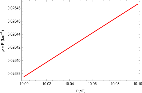
Figure 1: Variation of the pressure or the matter density $\rho=p$ ($km^{-2}$) of the shell with respect to r for $M=3.75M_{\odot}$ (taking $\xi=0.235$, $\rho_{0}=0.01$)

.

5.2 Proper length

According to the conjecture of Mazur and Mottola, the stiff fluid of the shell is situated between the junction of two spacetimes. The length span of the shell is from $R_{1}=R$ ($\it i.e.,$ the phase boundary between the interior and the shell) to $R_{2}(=R+\epsilon)$ ($\it i.e.,$ the phase boundary between the shell and the exterior spacetime), where $\epsilon<<1$. So, one can calculate the proper thickness between these two interfaces and the proper length or the proper thickness of the shell can be determined using the following formula:

$$\ell=\int_{R}^{R+\epsilon}\sqrt{e^{\mu}}dr=\int_{R}^{R+\epsilon}\frac{dr}{\sqrt{-12\xi\ln(r)+2\ln(r)+C_{3}}}.$$ (5.2)

To solve the above equation, let us consider that $\frac{df(r)}{dr}=\frac{1}{\sqrt{e^{-\mu}}}$, so that we get

$$\ell=\int_{R}^{R+\epsilon}\frac{df(r)}{dr}dr=f(R+\epsilon)-f(R)=f(R)+\epsilon f^{\prime}(R)+\frac{\epsilon^{2}}{2!}f^{\prime\prime}(R)-f(R)=\epsilon f^{\prime}(R)+\frac{\epsilon^{2}}{2!}f^{\prime\prime}(R).$$ (5.3)

In order to calculate the thickness of thin shell we have adopted the thin shell approximation and restricted upto second order term of thickness parameter $i.e.,$ the order of $\epsilon^{2}$ and eventually we have obtained the proper thickness of the shell as

$$\ell=\int_{R}^{R+\epsilon}\sqrt{e^{\mu}}dr=\frac{1}{2}\frac{-24\epsilon(\xi-\frac{1}{6})R\ln(R)+{\epsilon}^{2}(6\xi-1)+2R\epsilon C_{3}}{\left((-12\xi+2)\ln(R)+C_{3}\right)^{3/2}R}.$$ (5.4)

Variation of proper length within the thin shell has been shown in Fig. 2. The plot shows that the proper length increases monotonically with the increase of the thickness of the shell.

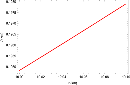
Figure 2: Proper length $\ell$(km) of the shell is plotted with respect to the radial distance of the shell $r$ (km) for $M=3.75M_{\odot}$ (taking $\xi=0.235$).

5.3 Energy

In the interior region as we consider the EOS, $p=-\rho$, one can argue that this indicates the negative energy region confirming the repulsive nature of the core. However, the energy within the shell and can be found out to be The energy $E$ within the shell can be calculated as

$${\it E}=\int_{R}^{R+\epsilon}4\pi r^{2}\rho dr={\frac{4(6\xi-1)^{2}\pi\rho_{0}}{156\xi^{2}-64\xi+7}\left[r^{{\frac{156\xi^{2}-64\xi+7}{(6\xi-1)^{2}}}}\right]_{R}^{R+\epsilon}}$$ (5.5)

Variation of the energy over the thin shell has been shown in Fig. 3. This figure demonstrates that the energy is increasing with the increment of thickness of the shell.

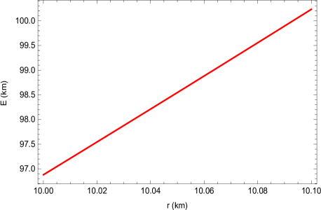
Figure 3: Energy E (km) within the shell is plotted with respect to the radial distance of the shell $r$ (km) for $M=3.75M_{\odot}$ (taking $\xi=0.235$, $\rho_{0}=0.01$).

5.4 Entropy

Following Mazur and Mottola prescription [1], we can determine the entropy of the thin shell using the following equation,

$$S=\int_{R}^{R+\epsilon}4\pi r^{2}s(r)\sqrt{e^{\mu(r)}}dr$$ (5.6)

where $s(r)$ is the entropy density for local temperature $T(r)$ and can be written as

$$s(r)=\frac{\alpha^{2}k_{B}^{2}T(r)}{4\pi\hbar^{2}}=\alpha\left(\frac{k_{B}}{\hbar}\right)\sqrt{\frac{p}{2\pi}}$$ (5.7)

where $\alpha$ is a dimensionless constant. Here we have assumed in the Planckian units, i.e., $k_{B}$ = $\hbar$ = 1 along with the geometrized units, i.e., $G=c=1$ as mentioned earlier. In order to calculate the entropy of system we have adopted the thin shell approximation and restricted upto second order term of thickness parameter $i.e.$ order of $\epsilon^{2}$ and the entropy of the fluid within the shell can be given by,

$$S(R) = \frac{\sqrt{\pi}\alpha k_{B}\sqrt{2}}{h}\left[\epsilon\sqrt{{\frac{\rho_{0}{R}^{4{\frac{(4\xi-1)(3\xi-1)}{(6\xi-1)^{2}}}}}{-12\xi\ln(R)+2\ln(R)+C_{3}}}}+\frac{\epsilon^{2}}{4}\left({\frac{4\rho_{0}(4\xi-1)(3\xi-1)R^{{\frac{4(4\xi-1)(3\xi-1)}{(6\xi-1)^{2}}}}}{(6\xi-1)^{2}r(-12\xi\ln(R)+2\ln(R)+C_{3})}}\right.\right.$$ (5.8)

$$\left.\left.-{\frac{\rho_{0}{R}^{4{\frac{(4\xi-1)\left(3\xi-1\right)}{(6\xi-1)^{2}}}}}{\left(-12\xi\ln(R)+2\ln(R)+C_{3}\right)^{2}}\left(-{\frac{12\xi}{R}}+\frac{2}{R}\right)}\right){\frac{1}{\sqrt{{\frac{\rho_{0}{R}^{{\frac{4(4\xi-1)\left(3\xi-1\right)}{(6\xi-1)^{2}}}}}{-12\xi\ln(R)+2\ln(R)+C_{3}}}}}}\right].$$

Following Ref. [21] it can be shown that (i) the thickness of the shell is negligibly small compared to its position from the center of the gravastar ($i.e.$, if $\epsilon<<R$), and (ii) the entropy depends on the thickness of the shell. Variation of entropy within the shell is shown in Fig. 4.

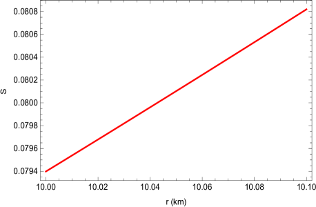
Figure 4: Variation of the entropy (S) of the shell with respect to $r$ for $M=3.75M_{\odot}$ (taking $\xi=0.235$, $\rho_{0}=0.01$).

6 Junction Condition

We know that gravastar consists of three regions, viz., interior (I), exterior (III) and intermediate shell (II). This shell maintains the connection between interior region ($I$) and exterior region ($II$). So it plays a very crucial part in the configuration of gravastar. This makes a geodetically complete manifold with a matter shell at the surface $r=R$. Thus a single manifold characterizes the gravastar configuration. At the junction there has to be a smooth matching between regions I and III, according to the fundamental junction condition. Though the metric coefficients are continuous at the junction surface but the derivatives of these metric coefficients may not be continuous there. Now we will use Darmois-Israel condition [73, 74, 75] to compute the surface stresses at the junction interface. The intrinsic surface stress energy tensor $S_{ij}$ is given by the Lanczos equation [76, 77, 78, 79] in the following form:

$$S_{j}^{i}=-\frac{1}{8\pi}\left[K_{j}^{i}-\delta_{j}^{i}K_{k}^{k}\right].$$ (6.1)

The discontinuity in the second fundamental form is given by

$$K_{ij}=K_{ij}^{+}-K_{ij}^{-}.$$ (6.2)

Here the second elemental form can be written as

$$K_{ij}^{\pm}=-\eta_{\nu}^{\pm}\left[\frac{\partial^{2}X_{\nu}}{\partial\zeta^{i}\partial\zeta^{j}}+\Gamma^{\nu}_{\alpha\beta}\frac{\partial X^{\alpha}}{\partial\zeta^{i}}\frac{\partial X^{\beta}}{\partial\zeta^{j}}\right]|_{S}$$ (6.3)

with the unit normal vector $\eta_{\nu}^{\pm}=\pm\left|g^{\alpha\beta}\frac{\partial f}{\partial X^{\alpha}}\frac{\partial f}{\partial X^{\beta}}\right|^{\frac{1}{2}}\frac{\partial f}{\partial X^{\nu}}$ with $\eta^{\nu}\eta_{\nu}=1$. Here $\zeta^{i}$ is the intrinsic coordinate on the shell and $f(X^{\alpha}(\zeta^{i}))=0$ is the parametric equation of the shell. Here $+$ and $-$ correspond to Schwarzschild spacetime and the interior spacetime of the gravastar respectively.

Considering spherically symmetric spacetime following Lanczos equation, the surface stress energy tensor can be written as $S_{ij}=diag(-\Sigma,P,P,P)$, where $\Sigma$ and $P$ are surface energy density and surface pressure respectively. The parameters $\Sigma$ and $P$ can be expressed by the following equations as

$$\Sigma=\left[-\frac{1}{4\pi R}\sqrt{f}\right]_{-}^{+},$$ (6.4)

$$P=\left[-\frac{\Sigma}{2}+\frac{f^{\prime}}{16\pi\sqrt{f}}\right]_{-}^{+}.$$ (6.5)

So, using the above two Eqs (7.6) and (6.5) we have obtained the surface energy density and surface pressure respectively as,

$$\Sigma={\frac{1}{12\pi R}\left(\sqrt{3R^{2}C_{1}+9}-\sqrt{9-{\frac{18M}{R}}-3\Lambda R^{2}}\right)},$$ (6.6)

$$\textit{P}={\frac{3}{8\pi R}\left({{\frac{\left(1-{\frac{M}{R}}-\frac{2\Lambda R^{2}}{3}\right)}{\sqrt{9-{\frac{18M}{R}}-3\Lambda R^{2}}}}}-{\frac{\frac{2}{3}{R}^{2}C_{{1}}+1}{\sqrt{3R^{2}C_{1}+9}}}\right)}.$$ (6.7)

Variation of the surface energy density is shown in Fig. 6. We have observed that both the parameters remain positive throughout the shell which immediately indicate that null energy condition has been satisfied for the formation of thin shell. Here, in Fig. 6, we have showed the variation of the surface energy density ($\Sigma$) for four different $\xi$ values taking mass of the gravastar $M=3.75M_{\odot}$ and $R_{1}=10.0$ km and thus we can predict the boundary of the intermediate shell ($R_{2}$) where the surface energy density ($\Sigma$) goes to zero for different $\xi$ values, which is first observed in our study. It is also evident that although surface energy density is more for lower $\xi$, it attains vanishing value earlier (say $\xi=0.28\;(Brown)$ in Fig. 6.

In Table-I, we have seen that the value of $R_{2}$ increases $i.e.,$ the thickness of the boundary increases for higher $\xi$ values of a particular star. There is a discontinuity of the second fundamental form at the junction between the two spacetimes which further implies that there must be a matter component (ultra relativistic fluid) obeying EOS $p=\rho$. This non-interacting matter or the fluid characterizes the existence of the thin shell of the gravastar.

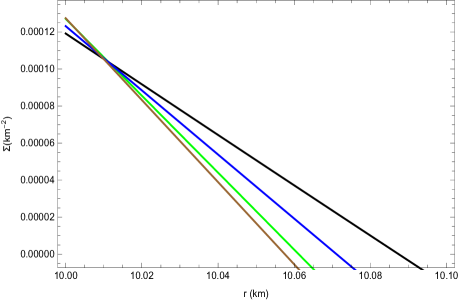
Figure 5: Variation of the surface energy density ($\Sigma$) ($km^{-2}$) of the shell with $r$ (km) taking $M=3.75M_{\odot}$ for different $\xi=0.228(Brown)$, $\xi=0.23(Green)$, $\xi=0.235(Blue)$ and $\xi=0.24(Black)$ values

Now, it is easy to find the surface mass $m_{s}$ of the thin shell from the equation of the surface energy density

$$m_{s}=4\pi r^{2}\Sigma=\frac{R}{3}\left(\sqrt{3R^{2}C_{1}+9}-\sqrt{9-{\frac{18M}{R}}-3\Lambda R^{2}}\right),$$ (6.8)

For negative $C_{1}$, we get a upper limit of radius $R<\sqrt{\frac{3}{|C_{1}|}}$ for which $m_{s}$ is realistic. Finally we note a limiting value on the radius

$$\left(\frac{6M}{\Lambda-|C_{1}|}\right)^{\frac{1}{3}}<R<\sqrt{\frac{3}{|C_{1}|}}$$

with $|C_{1}|<\Lambda$. The mass $M$, $\Lambda$ and $C_{1}$ determines the range of values of radius. It is interesting to note that the mass of a gravastar determines the lower limit of its size. With the help of the above equation we calculate the total mass of the gravastar in terms of the mass of the thin shell ($m_{s}$) as

$$M=\frac{2Rm_{s}\sqrt{3R^{2}C_{1}+9}-R^{4}(\Lambda+C_{1})-3{m_{s}}^{2}}{6R}.$$ (6.9)

7 Stability

In this section, we have studied the stability of our theoretical model by two methods: (i) Surface Redshift and (ii) Entropy maximization. The methods are described below:

7.1 Surface Redshift

Study of surface redshift of the gravastars can be considered as one of the most important source of information regarding it’s stability and detection. The surface gravitational redshift can be defined as $Z_{s}=\frac{\Delta\lambda}{\lambda_{e}}=\frac{\lambda_{0}}{\lambda_{e}}$, where $\Delta$ represents the fractional change in wavelength between the emitted signal $\lambda_{e}$ and observed signal $\lambda_{0}$. Buchdahl claimed that for an isotropic, static, perfect fluid distribution the value of surface redshift should not exceed $2$, $i.e.$, $Z_{s}<2$ [80, 81, 82]. Ivanov [83] claimed for anisotropic fluid distribution it can increase upto $3.84$. Barraco and Hamity [84] showed that $Z_{s}\leq 2$ for an isotropic fluid distribution when the cosmological constant is absent. But Bohmer and Harko [82] proved that in presence of cosmological constant of an anisotropic star $Z_{s}\leq 5$. To calculate the surface redshift we have used the following equation

$$Z_{s}=-1+\frac{1}{\sqrt{g_{tt}}}$$ (7.1)

eventually we get the surface redshift as,

$$Z_{s}=-1+\frac{1}{C_{4}^{\frac{1}{2}}\;r^{\left(\frac{2-6\xi}{6\xi-1}\right)}}$$ (7.2)

We have plotted the variation of surface redshift in Fig. 6. From the figure it can be observed that the value of $Z_{s}$ lies within 1 throughout the thin shell. So, our present model of gravastar can be claimed to be stable as well as physically acceptable.

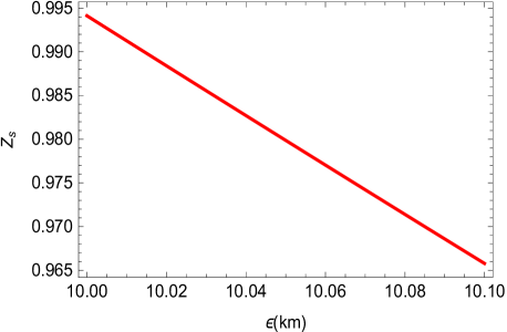
Figure 6: Variation of surface redshift of the shell with its thickness $\epsilon$ (km) for $M=3.75M_{\odot}$ (taking $\xi=0.235$).

7.2 Entropy maximization

Now to check the stability of the present study on gravastar in Rastall gravity we have followed the technique proposed by Mazur and Mottola [1, 2]. In order to accomplish this we have applied the technique of maximization of the entropy functional with respect to the mass function $M(r)$ and checked the sign of second variation of the entropy function. The first variation must vanish at the boundaries of the intermediate thin shell of the gravastar, which are fixed at $r=R_{1}$ and $r=R_{2}$ respectively i.e., $\delta S=0$

Now, the entropy functional can be written as

$$S=\frac{\sqrt{2}\alpha k_{B}}{2\hbar}\int^{R_{2}}_{R_{1}}rdr\left(\frac{dM}{dr}\right)^{\frac{1}{2}}\frac{1}{\sqrt{g(r)}},$$ (7.3)

here $g(r)=1-\frac{2M}{r}-\frac{\Lambda r^{2}}{3}$.

Now from Eqs. (3.11), (3.14) and (4.1) one can find the form of $M(r)$ in Rastall theory of gravity as

$$M(r)=-r\left((6\xi-1)\ln\left(\frac{R_{1}}{r}\right)+\frac{\Lambda{r}^{2}}{6}+\frac{C_{1}{R_{1}}^{2}}{6}\right).$$ (7.4)

Hence, we can obtain the second variation of the entropy function as

$$\delta^{2}S=\frac{\sqrt{2}\alpha k_{B}}{2\hbar}\int^{R_{2}}_{R_{1}}rdr\left(\frac{dM}{dr}\right)^{\frac{-3}{2}}\frac{1}{\sqrt{g(r)}}\left[-\left(\frac{d(\delta M)}{dr}\right)^{2}+\frac{(\delta M)^{2}}{g^{2}r^{2}}\left(\frac{dM}{dr}\right)\left(1+\frac{dM}{dr}\right)\right].$$ (7.5)

Here we have considered the linear combination of $M(r)$ as $\delta M=\beta\psi$, where $\psi$ vanishes at the boundaries. Now inserting this into Eq. 7.5, and integrating by parts keeping $\delta M=0$ at the extreme points of the thin shell, eventually we left with

$$\delta^{2}S=-\frac{\sqrt{2}\alpha k_{B}}{2\hbar}\int^{R_{2}}_{R_{1}}rdr\left(\frac{dM}{dr}\right)^{\frac{-3}{2}}\frac{1}{\sqrt{g(r)}}\beta^{2}\left[\frac{d\psi}{dr}\right]^{2}<0.$$ (7.6)

It clearly shows that, the entropy function in Rastal gravity attains the maximum value for all the radial variations which are vanished at the end points of the boundary of the shell of the gravastar. So we can conclude that the perturbation in the fluid of the intermediate shell region of the gravastar causes a decrease in entropy in the region II which is further indicating that our solutions are stable against small perturbations with fixed end points. In essence, the effect of modified gravity does not affect the stability of the gravastar.

8 Discussions and Conclusions

In the paper a unique stellar model of gravastar is studied following the conjecture of Mazur-Mottola in the Rastall’s theory of gravity. We obtain a set of exact, singularity free and physically acceptable solutions with a number of interesting and satisfactory properties of the gravastar in Rastall gravity. The following salient features of gravastar are noted :

(1) Interior region : Using the EOS given by Eq. (3.1) and the conservation equation Eq. (2.11) it is found that the matter density as well as the pressure remains constant in the interior. Again using field Eqs. (2.8)- (2.10), the metric functions $e^{\mu(r)}$ and $e^{\nu(r)}$ are determined. It is evident that both the functions are continuous at the origin $r=0$, and thus free from central singularity. We have also determined the active gravitational mass of the interior.

(2) Intermediate thin shell : In the intermediate thin shell region, one can apply the thin shell approximation and compute the corresponding metric functions. Both the metric functions remain finite and positive over the shell. The metric functions are modified due to the Rastall gravity effects which depend on the Rastall parameter $\xi$.

(3) Physical parameters of the Shell: Various physical parameters associated with the shell are computed which are modified in the Rastall gravity. The detail of the parameters are as follows:

(i) Pressure and matter density: The matter density or the pressure of the shell is plotted against the radial distance $r$ in Fig. 1. The variation of matter density or pressure for the shell is found to be positive which is monotonically increasing towards the exterior surface. This demands that the shell becomes more denser at the exterior boundary than the interior boundary.

(ii) Proper thickness: The proper thickness of the shell is determined adopting the thin shell approximation which is physically acceptable. The proper thickness or proper length $\ell$ of the shell is found to be monotonically increasing in nature from the interior junction to the exterior junction which is shown in Fig. 2.

(iii) Energy: The energy of the shell has been obtained in Eq. (5.5) and the variation with respect to radial parameter is shown in Fig. 3. The variation of energy is similar to that of the matter density. It satisfies the requirement that the energy of the shell increases with the increase in the radial distance.

(iv) Entropy: The entropy $S$ within the shell is given by Eq. (5.8) and the variation of entropy is shown in Fig. 4. The entropy is gradually increasing with respect to the radial distance $r$ indicating a maximum value of entropy on the surface of the gravastar which satisfies the physical validity condition. In order to calculate the entropy of the thin shell we assumed thin shell approximation and restricted upto second order term of thickness parameter $\epsilon$ ($i.e.,$ the order of $\epsilon^{2}$).

(4) Junction condition: The junction condition for the formation of thin shell between the interior and exterior spacetimes is considered. Following the condition of Darmois and Israel we study the variation of the surface energy density due to the formation of thin shell, which is plotted in Fig. 5 for different $\xi$ values. Both the parameters remain positive which indicates that the thin shell satisfies the weak and dominant energy conditions. In Fig. 5, we plot the variation of the surface energy density ($\Sigma$) for four different $\xi$ values taking mass of the gravastar $M=3.75M_{\odot}$ and $R_{1}=10.0$ km. This determines the variation of boundary of the gravastar with the Rastall parameter.

(5) Stability: The stability of the model is studied considering the surface redshift analysis and the entropy maximization technique. It is found that our model is stable and physically acceptable. It is found that :

(i) Surface redshift:The stability of the gravastar is checked using surface redshift analysis. For any stable stellar model the value of surface redshift lies within $2$. In the present case we have found that our model is stable under surface redshift analysis as can be noted from Fig. 6.

(ii) Entropy Maximization: We have checked the stability of gravastar models in Rastall gravity following the technique proposed by Mazur and Mottola [1, 2].We employ the maximization of the entropy with respect to the mass function $M(r)$ and checked the sign of second variation of the entropy for its consistency. Eq. (7.6) shows that the entropy function in Rastall gravity attains the maximum value for all the radial variations which are vanished at the end points of the boundary of the shell of the gravastar, perturbation in the fluid of the intermediate shell region of the gravastar causes a decrease in entropy in the region II which is further indicating that our solutions are stable against small perturbations with fixed end points.

(6) We have obtained the five different constants for different values of $\xi$ values which is shown in Table-I by choosing the mass of the gravastar $M=3.75M_{\odot}$ and interior radius $R_{1}=10$ km. In Table-II, we have also predicted the variation of the exterior boundary of the thin of shell ($R_{2}$) of the gravastar with the Rastall parameter ($\xi$). Thus we have examined the effect of Rastall gravity ($\xi$) in gravastar which is a new result.

(7) Again, we also find different metric parameters for a particular choice of $\xi=0.24$ by varying the mass value of gravastar which is shown in Table-II. For a given combination of $M$ and $R_{2}$ it would provide an unique solution, but we have chosen the values to satisfy the ratio $\frac{2M}{r}<\frac{8}{9}$ and $Z_{s}<2$ for a stable model.

From all the above analysis one can easily conclude that the gravastar may exist under the framework of Rastall’s theory of gravity. Unlike the previous works on gravastars, we have taken the thin shell approximation up to the second-order which provides more accurate results of the physical parameters of the shell. It is interesting to note that under the framework of of Rastall gravity the form of different physical parameters viz., energy, entropy, proper length etc. have been modified than those obtained in Einstein’s GR or other alternative gravity theories. One can get back the expressions of these parameters as obatained in Einstein’s GR by putting $\xi=0$ and restricting to the first-order approximation of the thickness parameter ($\epsilon$) of the shell. Also, unlike Einstein’s GR one can observe that the effect of Rastall gravity demands the exterior region of the gravastar to be de-Sitter type which is a clear indication of the existence of dark energy at the exterior region and its effect on the formation of stable gravastar under the framework of Rastall gravity.

8.1 Possibility of detection of gravastar:

Till date there are no direct evidences in favour of gravastar but few indirect evidences are available in the literature for predicting the existence and future detection of gravastar [5, 86, 85, 88, 89, 87, 90]. The concept for possible detection mechanism of gravastar was first proposed by Sakai et al. [85] through the study of gravastar shadows. Another possible method for the detection of gravastar may be employed by gravitational lensing method as suggested by Kubo and Sakai [85] where they have claimed that in a gravastar microlensing effects of larger maximal luminosity compared to black holes of the same mass might occur. According to Cardoso et al. [88, 89] the ringdown signal of GW 150914 [5] detected by interferometric LIGO detectors are supposed to be generated by objects without event horizon which might be a due to gravastar, though it is yet to be confirmed. Very recently in analysing the image obtained in the First M87 Event Horizon Telescope (EHT) result [91] it is not ruled out the possibility that the produced shadow may be due to gravastar. Shadow can be produced by any compact object having a spacetime which is characterized by unstable circular photon orbits as shown by Mizuno et al. [92]. According to Kubo and Sakai [85] gravastars can possess unstable circular photon orbits. In future, if similar effects mentioned above are detected observationally then it will be a good platform for comparing GR with Rastall gravity.

Analyzing the above points for our present study, we can conclude that, we obtain solutions in the Rastall theory of gravity which describe gravastars satisfactorily. For a gravastar in Rastall gravity an upper limit of radius is obtained determined by an integration constant $|C_{1}|<\Lambda$. We note a new result here that the mass of a gravastar determines its size. We have obtained a set of physically acceptable and non singular solution of the gravastar which immediately overcome the singularity problem and existence of event horizon of black hole. Analyzing we claim that our model of gravastar is stable under Rastall theory of gravity which is conceptually different from Einstein’s GR.

As a final comment we can say that, though there is no direct observational evidences are available till now which can differentiate a black hole from a gravastar. Again the recent observations of GW190521 clearly pointing out that the black hole theory is inconsistent with the observational results. Thus it can be argued that the possible black hole might be a possible gravastar.

9 Acknowledgements

SG and AD is thankful to the Department of Physics, IIEST Shibpur for providing research facilities and also thankful to Dr. Saibal Ray of G.C.E.C.T, Kolkata and Prof. B.K. Guha of Dept. of Physics, IIEST, Shibpur for their help and support. SG is also thankful to the Directorate of Legal Metrology under the Department of Consumer Affairs, West Bengal for their support. SD is thankful to UGC, New Delhi for financial support. The authors would like to thank IUCAA Centre for Astronomy Research and Development (ICARD), NBU for extending research facilities. AC would like to thank University of North Bengal for awarding Senior Research Fellowship. BCP would like to thank DST-SERB Govt. of India (File No.: EMR/2016/005734) for a project.

References

- [1] P. Mazur, E. Mottola, Gravitational Condensate Stars: An Alternative to Black Holes, Report number: LA-UR-01-5067 (2001) [gr-qc/0109035].
- [2] P. Mazur, E. Mottola, Gravitational vacuum condensate stars, Proc. Natl. Acad. Sci. USA 101 (2004) 9545. [gr-qc/0407075].
- [3] Y. B. Zel’dovich, The Equation of State at Ultrahigh Densities and Its Relativistic Limitations, Sov. Phys. JETP 14 (1962) 5, pg. 1143.
- [4] Y.B. Zel’dovich, A hypothesis, unifying the structure and the entropy of the Universe, Mon. Not. R. Astron. Soc. 160 (1972) 1P.
- [5] B. P. Abbott et al. (LIGO/Virgo Scientific Collaboration), Observation of Gravitational Waves from a Binary Black Hole Merger, Phys. Rev. Lett. 116 (2016) 061102. [gr-qc/1602.03837 ].
- [6] M. Visser and Wiltshire D. L., Stable gravastars - an alternative to black holes?, Class. Quant. Gravit. 21 (2004) 1135 [gr-qc/0310107].
- [7] C. Cattoen, T. Faber, M. Visser, Gravastars must have anisotropic pressures, Class. Quant. Gravit. 22 (2005) 4189. [gr-qc/0505137].
- [8] B.M.N. Carter, Stable gravastars with generalised exteriors, Class. Quant. Gravit. 22 (2005) 4551. [gr-qc/0509087].
- [9] N. Bilic et al., Born-Infeld Phantom Gravastars, JCAP 0602 (2006) 013. [astro-ph/0503427].
- [10] F. Lobo, Stable dark energy stars, Class. Quant. Gravit. 23 (2006) 1525. [gr-qc/0508115].
- [11] A. DeBenedictis et al., Gravastar Solutions with Continuous Pressures and Equation of State, Class. Quant. Gravit. 23 (2006) 2303 [gr-qc/0511097].
- [12] F. Lobo et al., Gravastars supported by nonlinear electrodynamics, Class. Quant. Gravit. 24 (2007) 1069. [gr-qc/0611083].
- [13] D. Horvat et al., Gravastar energy conditions revisited, Class. Quant. Gravit. 24 (2007) 5637 [gr-qc/0707.1636]
- [14] B.M.H. Cecilia Chirenti and L. Rezzolla , How to tell a gravastar from a black hole, Class. Quant. Gravit. 24 (2007) 4191 [gr-qc/0706.1513]
- [15] P. Rocha et al., Stable and ’bounded excursion’ gravastars, and black holes in Einstein’s theory of gravity, J. Cosmol. Astropart. Phys. 11 (2008) 010. [gr-qc/0809.4879 ].
- [16] D. Horvat, S. Ilijic and A. Marunovic, Electrically charged gravastar configurations, Class. Quant. Gravit. 26 (2009) 025003. [gr-qc/0807.2051].
- [17] A.A. Usmani, P.P. Ghosh, U. Mukhopadhyay, P.C. Ray, S. Ray, The dark energy equation of state, Mon. Not. R. Astron. Soc. 386 (2008) L92. [gr-qc/0801.4529].
- [18] B.V. Turimov, B.J. Ahmedov, A.A. Abdujabbarov, Electromagnetic Fields of Slowly Rotating Magnetized Gravastars, Mod. Phys. Lett. A 24 (2009) 733. [gr-qc/0902.0217].
- [19] K.K. Nandi et al., Energetics in condensate star and wormholes, Phys. Rev. D 79 (2009) 024011. [gr-qc/0809.4143].
- [20] T. Harko, Z. Kovcs and F. S. N. Lobo, Can accretion disk properties distinguish gravastars from black holes?, Class. Quant. Grav. 26 (2009) 215006. [gr-qc/0905.1355 ].
- [21] A.A. Usmani, F. Rahaman, S. Ray, K.K. Nandi, P.K.F. Kuhfittig, Sk.A. Rakib, Z. Hasan, Charged gravastars admitting conformal motion, Phys. Lett. B 701 (2011) 388. [gr-qc/1012.5605].
- [22] F. Rahaman et al., The - dimensional gravastars, Phys. Lett. B 707 (2012) 319. [gr-qc/1108.4824].
- [23] F. Rahaman et al., The - dimensional charged gravastars, Phys. Lett. B 717, 1 (2012) [gr-qc/1205.6796].
- [24] P. Bhar, Higher dimensional charged gravastar admitting conformal motion, Astrophys. Space Sci., 354 (2014) 457.
- [25] F. Rahaman, S. Chakraborty, S. Ray, A.A. Usmani, S. Islam, The Higher Dimensional Gravastars, Int. J. Theor. Phys. 54 (2015) 50. [gr-qc/1209.6291].
- [26] S. Ghosh, F. Rahaman, B.K. Guha, and S. Ray, Charged gravastars in higher dimensions, Phys. Lett. B 767 (2017) 380. [gr-qc/1511.05417].
- [27] S. Ghosh, F. Rahaman, B.K. Guha, and S. Ray, Gravastars with higher dimensional spacetimes, Ann. of Phys. 394 (2018) 230–243. [gr-qc/1701.01046].
- [28] S. Ghosh, S. Biswas, F. Rahaman, B.K. Guha, S. Ray, Gravastars in dimensions admitting Karmarkar condition, Ann. of Phys. 411 (2019) 167968.
- [29] S. Ghosh, D. Shee, F. Rahaman, B.K. Guha and Saibal Ray, Gravastars with Kuchowicz metric potential, Results in Physics 14 (2019) 102473.
- [30] R. Chan and M.F.A. da Silva, How the charge can affect the formation of gravastars, JCAP 07 (2010) 29 [gr-qc/1005.3703].
- [31] R. Chan, M.F.A. da Silva, Jaime F. Villas da Rocha and Anzhong Wang, Radiating gravastars, JCAP 10 (2011) 13 [gr-qc/1109.2062].
- [32] A.G. Riess et al., Observational Evidence from Supernovae for an Accelerating Universe and a Cosmological Constant, Astron. J. 116 (1998) 1009. [astro-ph/9805201].
- [33] S. Perlmutter et al., Measurements of and from 42 High-Redshift Supernovae, Astrophys. J. 517 (1999) 565.
- [34] P. de Bernardis et al., A flat Universe from high-resolution maps of the cosmic microwave background radiation, Nature (London) 404, 955 (2000). [astro-ph/0004404].
- [35] S. Hanany et al., MAXIMA-1: A Measurement of the Cosmic Microwave Background Anisotropy on angular scales of 10 arcminutes to 5 degrees, Astrophys. J. 545, L5 (2000). [astro-ph/0005123].
- [36] P. J. E. Peebles and B. Ratra, The cosmological constant and dark energy, Rev. Mod. Phys. 75, 559 (2003). [astro-ph/0207347].
- [37] T. Padmanabhan, Cosmological Constant - the Weight of the Vacuum, Phys. Rep. 380, 235 (2003). [hep-th/0212290].
- [38] T. Clifton, P. G. Ferreira, A. Padilla, and C. Skordis, Modified gravity and cosmology, Phys. Rep. 513, 1 (2012). [astro-ph/1106.2476].
- [39] A.G Riess et al, New Hubble Space Telescope Discoveries of Type Ia Supernovae at : Narrowing Constraints on the Early Behavior of Dark Energy, Astrophys. J. 659 (2007) 98. [astro-ph/0611572].
- [40] K. Tegmark et al, Cosmological parameters from SDSS and WMAP, Phys. Rev. D 69 (2004) 103501. [astro-ph/0310723].
- [41] R. Amanullah et al, Spectra and Light Curves of Six Type Ia Supernovae at and the Union2 Compilation, Astrophys. J. 716 (2010) 712. [astro-ph/1004.1711].
- [42] E. Komatsu et al, Seven-Year Wilkinson Microwave Anisotropy Probe (WMAP) Observations: Cosmological Interpretation, Astrophys. J. Suppl. 192 (2011) 18. [astro-ph/1001.4538].
- [43] A. Das, F. Rahaman, B. K. Guha and S. Ray, Relativistic compact stars in f(T) gravity admitting conformal motion, strophys. Space Sci. 358 (2015) 36 [gr-qc/1507.04959]
- [44] A. Das, F. Rahaman, B. K. Guha and S. Ray, Compact stars in f(R,T ) gravity, Eur. Phys. J. C 76 (2016) 654 [gr-qc/1608.00566 ].
- [45] A. Das, S. Ghosh, B.K. Guha, S. Das, F. Rahaman, S. Ray,Gravastars in f(R,T) gravity, Phys. Rev. D95 (2017) 124011.[gr-qc/ 1702.08873 ].
- [46] S. Biswas, S. Ghosh, B.K.Guha, F. Rahaman, S. Ray, Strange stars in Krori–Barua spacetime under f(R,T) gravity, Annals Phys. 401 (2019) 1 [gr-qc/ 1803.00442 ].
- [47] S. Ghosh, A.D. Kanfon, A. Das, M.J.S. Houndjo, I. G. Salako and S. Ray,Gravastars in f(T,T) gravity, Int. J. of Mod. Phys. A 35 (2020) 2050017.
- [48] A. Das, S. Ghosh, D. Deb, B.K. Guha, F. Rahaman and S. Ray,Study of gravastars under f (T) gravity, Nuc. Phys. B 954 (2020) 114986 [gr-qc/ 2003.10842 ].
- [49] R. Sengupta , S. Ghosh, S. Ray, B. Mishra and S. K. Tripathy,Gravastar in the framework of braneworld gravity, Physical Review D 102 (2020) 024037 [gr-qc/ 2004.01519].
- [50] S. Banerjee, S. Ghosh, N. Paul, F. Rahaman,Study of gravastars in Finslerian geometry, Euro. Phys. J Plus 135 (2020) 185.
- [51] P. Rastall, Generalization of the Einstein Theory, Phys. Rev. D 6 (1972) 3357.
- [52] P. Rastall, A Theory of Gravity, Can. J. Phys. 54 (1976) 66.
- [53] M. Capone, V.F. Cardone and M.L. Ruggiero, The possibility of an accelerating cosmology in Rastall’s theory, J. Phys. Conf. Ser. 222 (2010) 012012.
- [54] C. E. M. Batista, M. H. Daouda, J. C. Fabris, O. F. Piattella and D. C. Rodrigues, Rastall cosmology and the model, Phys. Rev. D 85 (2012) 084008. [astro-ph/1112.4141].
- [55] Y. Heydarzade, H. Moradpour and F. Darabi, Black Hole Solutions in Rastall Theory, Can. J. Phys. 95 (2017) 1253. [gr-qc/1610.03881].
- [56] Z. Haghani, T. Harko and S. Shahidi, The Einstein dark energy model, Phys. Dark Univ. 21 (2018) 27 [gr-qc/1707.00939]
- [57] Y. Heydarzade, H. Hadi, C. Corda and F. Darabi, Braneworld Black Holes and Entropy Bounds, Phys. Lett. B 776 (2018) 457 [gr-qc/ 1706.04434]
- [58] R. Kumar and S. G. Ghosh,Rotating black hole in Rastall theory, Eur. Phys. J. C 78 (2018) 750 [gr-qc/ 1711.08256]
- [59] Z. Xu and J. Wang, Kerr-Newman-AdS Black Hole Surrounded by Perfect Fluid Matter in Rastall Gravity, Eur. Phys. J. C 78 (2018) 513. [gr-qc/1711.04542].
- [60] M. S. Ma and R. Zhao, Noncommutative geometry inspired black holes in Rastall gravity, Eur. Phys. J. C 77 (2017) 629 [hep-th/1706.08054]
- [61] A. M. Oliveira, H. E. S. Velten, J. C. Fabris and L. Casarini,Neutron stars in Rastall gravity, Phys. Rev. D, 92 (2015) 044020 [gr-qc/ 1506.00567]
- [62] P. Bhar, F. Tello-Ortiz, Ángel Rincón, Y. Gomez-Leyton, Study on anisotropic stars in the framework of Rastall gravity, Astrophys. Space Sci. 365 (2020) 145.
- [63] P.C.W. Davies, Mining the Universe, Phys. Rev. D 30 (1984) 737.
- [64] J.J. Blome, W Priester, Naturwis. Vacuum energy in a Friedmann-Lemaître cosmos, Naturwissenschaften 71 (1984) 528.
- [65] C. Hogan, Cosmology: Cosmic strings and galaxies, Nat. 310 (1984) 365.
- [66] N. Kaiser, A. Stebbins,Nat.310 (1984) 391.
- [67] M.S. Madsen, J.P. Mimoso, J.A. Butcher, G.F.R. Ellis, Evolution of the density parameter in inflationary cosmology reexamined, Phys. Rev. D 46 (1992) 1399.
- [68] B.J. Carr, The Primordial black hole mass spectrum, Astrophys. J.201 (1975) 1.
- [69] I. Chakraborty, A. Pradhan, LRS BIANCHI I MODELS WITH TIME-VARYING GRAVITATIONAL AND COSMOLOGICAL CONSTANTS, Gravit. Cosmol. 7 (2001) 55.
- [70] T. Buchert,On Average Properties of Inhomogeneous Fluids in General Relativity: Perfect Fluid Cosmologies, Gen. Relativ. Gravit. 33 (2001) 1381 [gr-qc/0102049]
- [71] T.M. Braje, R.W. Romani, RX J1856A3754: EVIDENCE FOR A STIFF EQUATION OF STATE, Astrophys. J.580 (2002) 1043 [astro-ph/0208069v1]
- [72] L.P. Linares, M. Malheiro, S. Ray, THE IMPORTANCE OF THE RELATIVISTIC CORRECTIONS IN HYPERON STARS, Int. J. Mod. Phys. D 13 (2004) 1355.
- [73] G. Darmois,Memorial des Sciences Mathematiques XXV, Fasticule XXV, Gauthier-Villars, Paris, France, Chap. V (1927).
- [74] W. Israel, Singular hypersurfaces and thin shell in general relativity, Nuo. Cim. B44 (1966) 1.
- [75] W. Israel,erratum-ibid. 48 (1967) 463.
- [76] K. Lanczos, Ann. Phys. (Berlin) 379 (1924) 518.
- [77] N. Sen, Ann. Phys. (Leipzig) 378 (1924) 365.
- [78] G.P. Perry, R.B. Mann,Traversible wormholes in (2 + 1) dimensions Gen. Relativ. Gravit.24 (1992) 305 [gr-qc/0307034]
- [79] P. Musgrave, K. Lake,Junctions and thin shells in general relativity using computer algebra: I. The Darmois - Israel formalism, Class. Quant. Gravit.13 (1996) 1885 [gr-qc/9510052]
- [80] H. A. Buchdahl, General Relativistic Fluid Spheres Phys. Rev. 116 (1959) 1027.
- [81] N. Straumann, General Relativity and Relativistic Astrophysics, Springer, Berlin (1984).
- [82] C. G. Böhmer, T. Harko,Bounds on the basic physical parameters for anisotropic compact general relativistic objects, Class. Quantum Gravit.23 (2006) 6479 [gr-qc/0609061]
- [83] B.V. Ivanov, Maximum bounds on the surface redshift of anisotropic stars, Phys. Rev. D65 (2002) 104011 [gr-qc/0201090v2]
- [84] D.E. Barraco, V.H. Hamity, Maximum mass of a spherically symmetric isotropic star, Phys. Rev. D 65 (2002) 124028.
- [85] T. Kubo, N. Sakai, Gravitational lensing by gravastars, Phys. Rev. D93 (2016) 084051.
- [86] N. Sakai, H. Saida and T. Tamaki, Gravastar shadows, Phys. Rev. D 90 (2014) 104013 [gr-qc/1408.6929]
- [87] C. Chirenti and L. Rezzolla, Did GW150914 produce a rotating gravastar?, Phys. Rev. D 94 (2016) 084016 [gr-qc/1602.08759].
- [88] V. Cardoso, E. Franzin, and P. Pani, Is the Gravitational-Wave Ringdown a Probe of the Event Horizon?, Phys. Rev. Lett. 116 (2016) 171101 [gr-qc/1602.07309].
- [89] V. Cardoso, E. Franzin, and P. Pani, Erratum: Is the Gravitational-Wave Ringdown a Probe of the Event Horizon? Phys. Rev. Lett. 117 (2016) 089902.
- [90] N. Uchikata, S. Yoshida and P. Pani,Tidal deformability and I-Love-Q relations for gravastars with polytropic thin shells, Physical Review D 94 (2016) 064015.
- [91] EHT collaboration, First M87 Event Horizon Telescope Results. I. The Shadow of the Supermassive Black Hole, Astrophys. J. Lett. 875 (2019) L1 [astro-ph.GA/1906.11238]
- [92] Y. Mizuno et al., The current ability to test theories of gravity with black hole shadows, Nat Astron 2 (2018) 585 [astro-ph.GA/1804.05812]. .