GENETIC EVOLUTION OF A MULTI-GENERATIONAL POPULATION IN THE CONTEXT OF INTERSTELLAR SPACE TRAVELS
Part I: Genetic evolution under the neutral selection hypothesis

Abstract

We updated the agent based Monte Carlo code HERITAGE that simulates human evolution within restrictive environments such as interstellar, sub-light speed spacecraft in order to include the effects of population genetics. We incorporated a simplified – yet representative – model of the whole human genome with 46 chromosomes (23 pairs), containing 2110 building blocks that simulate genetic elements (loci). Each individual is endowed with his/her own diploid genome. Each locus can take 10 different allelic (mutated) forms that can be investigated. To mimic gamete production (sperm and eggs) in human individuals, we simulate the meiosis process including crossing-over and unilateral conversions of chromosomal sequences. Mutation of the genetic information from cosmic ray bombardments is also included. In this first paper of a series of two, we use the neutral hypothesis: mutations (genetic changes) have only neutral phenotypic effects (physical manifestations), implying no natural selection on variations. We will relax this assumption in the second paper. Under such hypothesis, we demonstrate how the genetic patrimony of multi-generational crews can be affected by genetic drift and mutations. It appears that centuries-long deep space travels have small but unavoidable effects on the genetic composition/diversity of the traveling populations that herald substantial genetic differentiation on longer time-scales if the annual equivalent dose of cosmic ray radiation is similar to the Earth radioactivity background at sea level. For larger doses, genomes in the final populations can deviate more strongly with significant genetic differentiation that arises within centuries. We tested whether the crew reaches the Hardy-Weinberg equilibrium that stipulates that the frequency of alleles (for non-sexual chromosomes) should be stable over long periods. We demonstrate that the Hardy-Weinberg equilibrium is reached for starting crews larger than 100 people, confirming our previous results, while noticing that larger departing crews (500 people) show more stable equilibriums over time.

Keywords: Long-duration mission – Multi-generational space voyage – Space exploration – Space genetics

1 Introduction

Why go explore exoplanets? One of the fundamental purposes of space exploration is the search for life other than the one we know on Earth. This question has obsessed humanity for thousands of years and is even found in ancient philosophical writings (Thales, Anaximander, Bruno, Kant …). The discovery of life on an extraterrestrial world within our Solar System, on an exoplanet or on an exomoon would, of course, be of prime interest. This would allow us to answer the fundamental question as to whether we (humans, and all other life forms found on Earth) are the only living beings in the Universe. In addition, such a discovery could also help better understand abiogenesis, that is the “natural generation” of life from non-living matter. Indeed, terrestrial life is based on a (bio)chemistry that involves only a few atoms: carbon, hydrogen, nitrogen, oxygen, phosphorus and sulfur (usually known through the mnemonic acronym CHNOPS). All those atoms are used by cells to construct simple to extremely complex high molecular mass molecules. Other trace elements (iron, zinc, potassium, sodium, boron, etc.) are also crucial to all living forms, although they are not integral part of macromolecules, but rather essential to the functioning of these molecular machines. Organic matter (carbon-containing molecules) now appears to be widespread in the Universe, including complex kinds of polymers, especially within meteorites [1], but the question of the origin of the first terrestrial complex molecular entities that underwent self-reproduction and used coordinated and complex chemical reaction networks (metabolism) to maintain their structural features remains a mystery. Moreover, are other types of chemistries (other than carbon-based) possible?

To answer these questions, satellites and rovers have been sent all over the Solar System. The wealth of planets, moons, asteroids and comets now explored tells us that potential living pools that could be suitable to life as we know it (Europa, Titan, Mars, see [2], [3], and [4], respectively) do exist. However, with the exception of Mars, none of the celestial bodies thus far explored within our Solar System seem to have kept for long enough periods of time conditions similar to those that presided on Earth when the first life forms are supposed to have emerged. Those facts make exoplanets and exomoons very interesting alternative candidates to study those questions. However, the tremendous distances between our planet and any exoplanet lead to missions taking centuries using non-fictional means of propulsion. This inevitably excludes deep-space exploration beyond the Solar System to first exploit resources for commercial or economic purposes, and rather highlights that it would necessarily be for other, likely scientific, goals.

One of the immediate consequences of those distances is that crewed journeys cannot be achieved within the life expectancy of a human. Discarding non-mature options (cryogenic technologies, suspended animation scenarios and genetic arks), the best choice might be to rely on giant self-contained generation ships that would travel through space while their population is active [5]. Such an undertaking requires choosing an initial crew in such a way that its overall genetic diversity be sufficient to sustain a long-term multi-generational voyage in an enclosed environment. Here, genetic diversity refers to the amount of variations that are present on average within the population that would minimize inbreeding and consanguinity, under the enclosed and isolated conditions that the crew and all subsequent offspring will endure during the course of space travel. Inbreeding and consanguinity have well-documented consequences on health [6] and fertility [7]. This directly impacts the population’s genetic health, which constrains the choice of a minimal viable population (MVP) [8, 9]. In addition, since migration back to or forward from Earth would be impossible given timescales and technological costs, the space-faring crew should be regarded as an ever after enclosed and henceforth isolated population, with no possible external genetic input. In this context, choosing an initial crew is complex because we need to introduce enough genetic variations in the spaceship’s population to avoid the genetic diversity to decrease with time, to the extent that inbreeding and consanguinity eventually prevails.

In our agent based Monte Carlo code HERITAGE [10, 11, 12, 13], because no genotype was formerly attributed to individuals, we took advantage of the precisely defined genealogy and kinship of individuals in the crew to evaluate the dynamics of consanguinity using the coefficients of inbreeding ($C_{\rm i}$) and of consanguinity ($F$) introduced by Wright [14]. They take into account only relationships of father/mother couples to their common ancestor at the generations scale [14]. The minimal number of initial crew members (male/female-balanced) that ensured $F$ to remain below a given security threshold expected not to be deleterious for the enclosed population was of $\sim$ 100 people to ensure a thousand year-long journey to Proxima Centauri $b$ [11]. As stated, $Ci$ and $F$ do not take into account genetic features of the initial crew that was presupposed to be genetically diverse (with low genetic similarities at the population level). However, because of a mechanism called genetic drift, the genetic composition of a starting population has to be taken into account to more realistically evaluate the evolution of inbreeding over time in an enclosed environment. This is what Smith [15] did when he applied population genetics probabilistic principles to determine a MVP of 14000 – 44000 individuals to have a healthy group of settlers upon a 5 generation-long journey. To this end, he followed the principle of reduction in heterozygosity (ROH, that is a measure of genetic diversity) applied to one single genetic element. ROH has effects similar to consanguinity in terms of health and reproductive outcomes [16] and accordingly affects the genetic health of a population [17].

The discrepancies between Smith’s and our results as to determine the MVP of the spaceship likely originates from the use of different methodologies that either integrate only kinship or simplified probabilistic population genetics principles that cannot alone approximate the complexity of population genetics at the genome scale. We therefore reasoned that to understand, quantify, evaluate and predict the complex genetic phenomena involved, we needed virtual populations in which individuals are endowed with bona fide genetic features mimicking those found in human genomes to perform forward-in-time population genetics simulations. Those are the goals of the present paper and its forthcoming accompanying publication (part II).

2 Adding genetics to HERITAGE

In order to include a representative model of the human genome and its evolution through multiple centuries of space travel – that, in addition, follow the laws of heredity and genetics –, we gradually improved HERITAGE. In the following, we detail the many upgrades of HERITAGE that will allow us to build increasingly realistic initial populations to simulate genetic outcomes of space-faring demes. In Sec. 2.1 we present the methodology to include chromosomes, loci and alleles in HERITAGE. In Sec. 2.2 we show how initial population genetics (the zeroth-generation) can be modeled. In Sec. 2.3 we describe the principles for transmitting the genetic traits from the parents to the offspring through gamete production and meiosis. We use this improvement to show the impact of allelic gene crossing-over and conversion onto the population genomes before including the effects of mutations and cosmic ray radiation in Sec. 2.4 and Sec. 2.5, respectively.

2.1 Methodology

2.1.1 The human genome: how to model it?

As stated in the introduction, a genealogical approach to measure the degree of consanguinity of individuals is a good way to evaluate the genetic diversity and health at the population level. However, the degree of genetic relatedness – that can lead to consanguinity in the offspring over time in small populations – strongly depends on the starting genetic composition of the initial population. It can be a continuum between high and low values, something that was not taken into account in our previous studies. In addition, the randomness of mating histories of and between individuals within genealogical lines can significantly modify the genetic composition (e.g., the frequency of alleles) of the overall descendant population throughout generations. This stochastically changes the degree of genetic relatedness between individuals, a phenomenon that not only depends on these individual histories, but also on the population’s size at each step. In order to better simulate human populations during the course of the interstellar journey by taking into account the genetic constitution of individuals and of the overall population, we needed to provide individuals with virtual genomes.

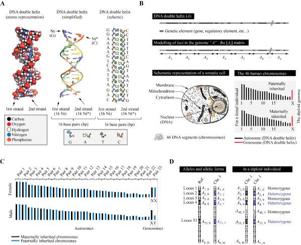
Figure 1: Model of the human genome such as implemented in HERITAGE. Description of the figure can be found in the text. Nt: (deoxyribo)nucleotide, Nt^∗: complementary Nt. A somatic (non-sexual) cell is represented to emphasize the nuclear localization of chromosomes within cells (in the nucleus).

Chromosome Size (x10⁶ base pairs) Number of genes (N) N/10 N/50 Simulated number of loci per chromosome 1 248.96 5096 509.6 101.92 100 2 242.19 3867 386.7 77.34 70 3 198.3 2988 298.8 59.76 60 4 190.22 2438 243.8 48.76 50 5 181.54 2594 259.4 51.88 50 6 170.81 3014 301.4 60.28 60 7 159.35 2770 277 55.4 55 8 145.14 2170 217 43.4 40 9 138.4 2265 226.5 45.3 40 10 133.8 2179 217.9 43.58 40 11 135.09 2921 292.1 58.42 60 12 133.28 2531 253.1 50.62 50 13 114.36 1378 137.8 27.56 30 14 107.04 2061 206.1 41.22 40 15 101.99 1822 182.2 36.44 35 16 90.34 1941 194.1 38.82 40 17 83.26 2449 244.9 48.98 50 18 80.37 984 98.4 19.68 20 19 58.62 2491 249.1 49.82 50 20 64.44 1358 135.8 27.16 30 21 46.71 777 77.7 15.54 15 22 50.82 1187 118.7 23.74 25 X 156.04 2186 218.6 43.72 45 Y 57.23 579 57.9 11.58 12 mitochondria 0.02 37 3.7 0.74 0 Total 3088.32 54083 1067

Table 1: Number of simulated number of loci per chromosome.

Let us first precisely define what “genome” means. In biology, the genome is referred to as the complete set of genetic elements of a given organism – here humans. In all known cellular organisms, the genetic material is composed of deoxyribonucleic acid (DNA), which is the shelf of the genetic information. This macromolecule, see Fig. 1 (A), is composed of two strands coiled together in a well-known double helix structure. Each strand is made of chains of building blocks called deoxyribonucleotides (that, for convenience, we shall term “nucleotides”, even if this is not chemically rigorous), whose succession constitutes the strand sequence. Nucleotides (A, T, G, C) found on one strand associate with complementary nucleotides on the opposite strand (A with T, G with C and reciprocally) to form so-called base pairs (bp) that contribute to the double helix’s stability. Because of this complementarity, complete knowledge of one strand sequence also provides complete knowledge of the second. This will facilitate our simulations, since only the “virtual sequence” of one strand shall be considered. DNA carries genetic elements (informational sequences) that can be genes – i. e. sequences that contain the instructions to synthesize proteins or non-coding ribonucleic acids –, but also regulatory sequences – i. e. that participate in the control and modulation of gene expression in response to internal and/or external stimuli –, or other types of elements. The human genome is composed of 3 $\times$ 10⁹ bp (two base-paired complementary strands of 3 $\times$ 10⁹ nucleotides each) and typically encodes $\sim$ 22 000 protein genes and approximatively the same number of non-coding RNA (ribonucleic acids) genes, see Tab. 1. Genetic elements are found at defined positions along the DNA molecule and, to simplify, we shall consider that these are discrete and non-overlapping, even though reality is more complex. The degree of complexity as to model these genetic elements to mirror the human genome is far beyond the scope of this study and well beyond computing possibilities.

A straightforward method to simulate a simplified human genome is to use matrices: let A₁, A₂, … A_n be the set of individual positions along the DNA molecule “A”. Those positions represent discrete and bounded blocks that are independent of each other in the sense that we can distinguish them by a property (their sequence, for example). As in genetics, a “bounded block” (of sequence) shall be termed a locus (plural loci). Loci can in principle either be considered nucleotide sequence intervals of any length, meaning that they can represent and/or contain any genetic feature or combination of genetic elements that are present on DNA. Their position on the chromosome is indexed in the order of their sequence by the letter $i$. We thus can create a matrix of one column and $n$ rows, where each line represents a particular locus. For A we thus have [A_i]=(A₁, A₂, A₃, A₄ … A_n), as shown in Fig. 1 (B).

2.1.2 Modeling the diploid genome and chromosomes

Humans are diploids, meaning that each human cell actually carries two genomes. One copy (a so-called haploid genome of $\sim$ 3 $\times$ 10⁹ bp) is of maternal origin, while the second haploid genome ($\sim$ 3 $\times$ 10⁹ bp) is of paternal origin. An individual’s diploid genome ($\sim$ 6 $\times$ 10⁹ bp) is the result of the combination of both. As shown in Fig. 1 (C), the human diploid genome is in fact separated into 46 physically independent DNA segments (double helices) that are called chromosomes: 23 of paternal origin and 23 of maternal origin. Among them, 22 paternal chromosomes and their 22 maternal counterparts are homologous, meaning that they are almost identical in terms of sequence, and conceptually grouped into 22 pairs of homologous chromosomes (autosomes). As an illustration, maternal chromosome 1 has its homologous paternal chromosome 1 counterpart – they share highly related sequence features – and so on for chromosomes 2 to 22. The two remaining are sexual chromosomes (gonosomes). In humans, females carry two homologous X sexual chromosomes (XX), while males possess one X and one small male-specific Y chromosome (XY) that are non-homologous (they differ in term of sequence, length, architecture, genetic elements content, etc.). Each chromosome carries its own set of genetic elements arranged along the sequence. Therefore, each chromosome can be modeled with a matrix of the same form as described above: for the first chromosome “A” we have [A_i]=(A₁, A₂, A₃, A₄ … A_n). For the second chromosome “B”, we have [B_i]=(B₁, B₂, B₃, B₄ … B_n) and so forth. Since each chromosome has one homologue, it implies that genetic elements (loci, sequence features, etc…) are always found in two copies within cells (one of maternal the other of paternal origin), with the exception of males, for which X- and Y-specific genes are present in single copies. Chromosome A thus has its A’ homologue, represented with matrix [A’_i]=(A’₁, A’₂, A’₃, A’₄ … A’_n), B has its homologous B’ chromosome represented with matrix [B’_i]=(B’₁, B’₂, B’₃, B’₄ … B’_n), etc. The complete human genome of a single individual can thus be numerically modeled using 46 individual matrices that we store in a single C++ vector, i.e. the diploid genome.

2.1.3 Genetic variations and alleles

The genetic information of human individuals is never rigorously identical (they are not clones). Genetic variations exist between individuals and between human populations that originate from past mutations that, by descent, were transmitted to the offspring. One consequence is that in one individual, the two haploid genomes inherited from his/her parents are not identical. If one considers a given locus A_i at a given position $i$ in a haploid genome (on chromosome A, for instance), it can have a given form (sequence), but another sequence (carrying variations of any type in various proportions) in another haploid genome (on the homologous chromosome A’). The two loci (A_i and A’_i) are the same genetic information, but with different states that are termed allelic forms. The two loci are termed alleles (or allelic forms) to one another. A given locus can have one or multiple possible allelic forms within a population. Let A₁₁, A₁₂, …, A_1m be the $m$ allelic forms that the first locus of A can take. The matrix [A_ij] therefore represents all the possible variants of all the loci found along A within the population, see Fig. 1 (D). The set of possible alleles of all the loci of chromosome A is thus an $n$ $\times$ $m$ matrix, with $n$ the number of loci (blocks) along A and $m$ the number of allelic forms of a given locus. The same can be applied to the homologous chromosome A’. A haploid genome can thus be considered a combination of specific alleles in a given order, that we shall term a haplotype. Each individual is diploid, and carries two haploid genomes – and, strictly speaking, two haplotypes –, a combination that is named a genotype (combination of alleles in a diploid individual).

2.1.4 The virtual human genome

As stated above, the human haploid genome is composed of 3 $\times$ 10⁹ bp and contain $\sim$ 22 000 protein genes and an almost equivalent number of non-protein genes. Due to the memory-space limitations of modern computers, it is challenging to allocate several thousands of vectors that each contains 46 $\times$ 2 $\times$ 22 000 $\times$ $m$ integer values if we would consider 22 000 blocks (corresponding to protein genes) on each haploid genome. The task would be even more challenging if individual nucleotides had to be taken into account (6 $\times$ 10⁹). We thus reasoned to approximate the human genome with a scaled-down model in order to keep the computing time reasonable. We therefore arbitrarily separated the sequences of each individual chromosome into N discrete blocks (where N corresponds to the number of genes of each chromosome divided by 50, see Tab. 1, fifth column), so the number of blocks became downscaled to 2110 for the entire diploid genome, with 100 loci for the largest chromosome (chromosome 1). Therefore, the human haploid genome of 3 $\times$ 10⁹ bp is, in our model, constituted of 1055 sequence blocks that, for convenience, we also termed loci. In this way, each locus/block can alternatively be considered a single gene, a set of genes, or any given DNA sequence of any size with specific and defined characteristics, depending on the scale to be considered. We thus included in the Human C++ class of HERITAGE (the blueprint of each numerical individual) a vector of 2110 integer values that is representative of the human genome (accounting for the homologous chromosomes). This vector will be filled upon the creation of the crew member, either at the beginning of the simulation or during the interstellar travel when reproduction will happen. The genome of each individual is stored by the program so that statistical and biological tests can be performed during and after the completion of the simulation. The typical memory-size of one human genome stored on the computer is 4.2 ko (34.4 kb). Note that the 1055 loci are distributed in a given order onto 23 chromosomes and that this architecture never changes. In reality, it is not strictly the case, but for simplicity we imposed the architecture of genomes (order and number of loci, number of chromosomes) to remain constant.

2.1.5 Measuring genetic diversity

A single human individual, because he/she carries two haploid genomes (he/she is diploid) independently acquired from the two parents, can carry two identical copies of a given locus (the same allele), or two different forms (alleles) of this locus. In the former case, the individual is termed homozygous at this locus/position, while in the latter case, it is referred to as heterozygous at this position/locus (Fig. 1 D). For each individual, we can therefore measure, at each locus A_ij, if he/she is heterozygous (carries two different alleles on chromosome A and A’) or homozygous (carries two identical alleles on A and A’). From this, we can measure the individual heterozygosity I_k of the k^th individual that is the fraction of pairs of homologous loci (A_ij and A’_ij) that are heterozygous. In the case of inbreeding, I_k is expected to decrease, because two closely related individuals (that share strong similarities in terms of allelic combinations) tend to produce descendants that are highly homozygous (reduced heterozygosity). In this sense, I_k is a measure of the genetic diversity at the individuals’ scale that will be used to evaluate inbreeding, consanguinity or similar phenomena that could arise from population genetics in individuals.

In addition, individual loci (A_ij) can have one or more allelic forms within a population. If the locus under investigation has more than one allelic form in the population, it is termed polymorphic. The degree of polymorphism (P) represents the fraction of loci (among the total N loci) that are polymorphic at the population scale. The allelic diversity (number of possible alleles) and the frequency of each allelic form within the whole population also have to be taken into account, because they both influence the proportion of possible heterozygous or homozygous individuals at various positions of the genome.

Finally, the heterozygosity index (H_i) measures the proportion of individuals that are heterozygous at position $i$ on locus A_i. Since the proportion of heterozygous individuals (at a given position $i$) depends on the actual allelic diversity (number and frequency of allelic forms at position $i$), it is also a measure of the genetic (allelic) diversity in the population. For $m$ allelic forms of a given locus, there are $m$ possible homozygous and $m$($m$-1)/2 heterozygous pairs that can exist in individuals. H_i depends on the number of possible alleles and their respective frequencies in the population. H_i is maximal (allelic diversity is maximal) when all allelic forms at position $i$ are equifrequent, with H_i,max,m=1-(1/$m$) at locus A_i. As indicated before, inbred or consanguineous populations tend to produce individuals that possess, on average, more homozygous positions than non-inbred populations, meaning that H_i is expected to decrease at discrete positions of the genome in the case of inbred populations, a phenomenon known as the Reduction in Heterozygosity (ROH) that Smith used, for one single locus, to evaluate the MVP of an interstellar journey [15]. In HERITAGE, we can now map H_i at all loci along the genome (except for sexual chromosomes) to visualize genome-scale changes in the genetic diversity of the population upon interstellar travels.

2.2 Building the initial population

The selection of the zeroth-generation for multi-generational space travels is of prime importance. First of all, one must realize that neither the initial crew members, nor most of the forthcoming generations, would reach the spaceship’s final destination. It means that they would be born, raised, live, have children, and die within the limited and enclosed environment offered by the vessel without any possibility for leaving this protective shell or tread upon the surface of a planet, hospitable for human life or not, before arrival. Long-duration off-Earth space missions within the Solar System (to the Moon or Mars) are already expected to cause strong emotional, psychological and psycho-pathological effects due to isolation and confinement but also to inter-personal, organizational and cultural aspects [19, 20, 21, 22, 23]. Such a series of constraints would undoubtedly be even stronger and more profound for people traveling beyond the Solar System, simply because interstellar travel implies to cross unthinkable distances. Spaceship system failure, exposure to on-board pathogens, radiation, social conflicts, external accidents, etc., would drive people, agencies or governments in charge of interstellar space exploration to select initial crew members with mental and psychological abilities that could best-fit such long-term constraints. Moreover, remoteness might favor the rise of a novel space culture with its own sociological, political, cultural, ethical – and possibly linguistic – properties and references [24, 25, 26, 15, 27], which would preclude any a priori (and unattainable) attempt to “socially engineer” an initial crew on the very long term.

Multi-generational space travel also raises biological issues regarding genetic diversity and health. In our case, “genetic diversity” shall refer, as we stated before, to the allelic diversity within the entire population enclosed in the vessel. It is described by the degree of polymorphism (P), the heterozygosity index of individuals (I_k) and the locus heterozygosity index (proportion of heterozygous individuals) at each locus (H_i). A “genetically diverse” population is ideally polymorphic, with a significant proportion of loci with multiple allelic forms that ensure that H_i does not approaches 0 (a case arising when only one allele exists in the population at position $i$), implying that heterozygous positions can exist, and that I_k remains high (individuals have multiple heterozygous positions). Note that, if P is high, a high proportion of all loci are polymorphic (have two or more allelic forms), which enables individuals to be heterozygous at various positions (increased I_k), and increases the chances that a given locus be heterozygous at the population scale (measured with H_i, the proportion of individuals that are heterozygous at position $i$).

Why should polymorphism and heterozygosity not become too low? We already indicated that inbreeding and consanguinity, that both reduce allelic diversity and, consequently, heterozygosity (both I_k and H_i), have well-documented consequences on health [6] and fertility [7]. This comes from the fact that, when genetically alike individuals reproduce, they produce descendants with genomes that correspond to the pooling of two genetically alike haploid genomes (see below), leading to multiple homozygous positions along the diploid genome. Some allelic variations (that originate from past mutations) can have deleterious manifestations (phenotypes) in individuals. The effect of such variations depends on the zygosity: deleterious dominant mutations manifest when individuals are homozygous (two identical mutated copies of the genetic element are present) or heterozygous (one mutated copy of the genetic element and one copy that does not possess the same mutation), while deleterious recessive mutations have effects only when individuals are homozygous (two mutated copies). Cystic fibrosis is an example of a recessive genetic variation that provokes a so-called genetic disease in homozygous but not in heterozygous individuals [28], but many others exist. When genetic diversity decreases, such as in the case of inbreeding and consanguinity, heterozygosity tends to decrease within the population, with homozygous positions increasing accordingly in individuals. This also increases risks to reveal deleterious recessive genetic effects/diseases. All possible homozygous combinations do not necessarily occur within a natural population with a large number of individuals, and associated recessive phenotypes (deleterious or not) therefore never or rarely manifest (from combinatorial). Therefore, even if chosen “genetically diverse”, the initial crew should, in addition, include enough individuals to avoid the next generations to be affected by inbreeding and consanguinity [10, 11] that both cause I_k and H_i to decrease. I_k and H_i can also be affected by strong stochastic variations in allele frequencies that could lead to random fixation (one allele becomes the only allelic form) or loss of alleles, due to a reduced number of possible mating combinatorial [15], a process that is referred to as “genetic drift” [29]. Since the initial crew will necessarily be small (limited resources, space, etc.), this will restrict mating possibilities between individuals and potentially affect I_k and H_i (reduce heterozygosity) and lead to inbreeding and/or consanguinity.

The initial crew would thus be regarded as a minimal viable population (MVP) [8, 9], in which genetic diversity (P, I_k and H_i) and the number of individuals would have to be determined to reduce risks of loss of heterozygosity (decrease of I_k and H_i) and consequently of inbreeding and consanguinity. In order to “stabilize” a selected initial allelic diversity in the initial population, the number of individuals shall be sufficient to reach, or at least approach, the Hardy-Weinberg equilibrium, a state under which alleles frequencies remain stable throughout generations within the population [30], which should also stabilize P, I_k and H_i.

The selection process of initial crew members could integrate tests to choose “genetically-healthy” candidates with no known deleterious genetic variations. In comparison to psychological tests, DNA sequencing technologies, clinical and genetic tests could more easily help determine whether the candidate or her/his offspring carry one or several genetic markers linked to known genetic disorders. However, things are far from being that simple:

• First, mutations in genes or genetic elements that generate allelic diversity can, of course, be detrimental to health, with phenotypes that express as well-known hereditary/congenital diseases. These genetic variations could, in principle, be excluded from the initial population to avoid highly deleterious genetic disorders. However, even if they were, de novo spontaneous mutations could put them back into the population’s allelic pool during the course of the journey, especially those that are known to occur with high frequencies on Earth.

• Second, mutations that are known to be associated with deleterious phenotypes can produce highly variable phenotypes (biological manifestations) in various individuals, depending on their own genetic background (genotype) [31, 32]. If the mutation of a genetic element is dominant, its associated phenotype will express even if only one of the two copies in the diploid genome is mutated; however, if it is recessive, only those individuals that possess two mutated copies will express the phenotype. This implies that novel homozygous combinations, naturally arising in the spaceship or originating from inbreeding and/or loss of heterozygosity could reveal unanticipated and unpredictable phenotypes, including diseases that, by definition, could not be detected as such when the initial population is constituted. In addition, the effect of a given dominant or recessive mutation not only depends on the hetero- or homozygous state of an allele, but also on the overall genetic background of individuals, that is, on other variations that are present across the diploid genome of an individual and that influence phenotypical manifestations. The same mutation can thus be entirely neutral (no phenotypical or fitness effect), advantageous or deleterious at various degrees depending on individuals’ genetic compositions. Cystic fibrosis [28] is affected by such genetic influences that modify clinical outcomes and severity of the disease [33], but this is true for any phenotypical trait.

• Third, gene expression strongly depends on the environment (temperature, pressure, gravity, pollution, diet, quality and amount of food, radiation, stress, etc.) or developmental stage of an individual. The manifestation of a phenotype associated with a given mutation therefore depends on the expression pattern and timing of the mutated gene, but also on the effect that it has on the capacity of the gene’s expression product (protein, RNA) to fulfill its function. Also, mutations in regulatory genetic elements can modify the expression pattern of one to several (sometimes hundreds of) genes in response to environmental, hormonal (external) or cellular (internal) signals and lead to unpredictable phenotypes, depending on what regulatory circuit and/or tissue, cell type is/are affected. Combined with the effect of the genetic background (other variations), one can understand that the effect of mutations and/or combination of mutations (or alleles) is not easy – and strictly speaking, impossible – to predict for one individual and, moreover, for an entire population [31, 32]. Since environmental conditions influence phenotypes, prediction of the effect of mutations on health, fertility or life expectancy is highly uncertain. This is also true for already existing genotypes, with known associated phenotypes (on Earth), that will be placed under novel environmental conditions (spaceship) and likely for all possible novel genetic combinations (genotypes).

From those facts it is clear that it would be almost impossible to predict or anticipate the rise of novel phenotypic manifestations (deleterious, neutral or advantageous) on-board. That is to say, it would be merely impossible to begin with a set of starting individuals (and genomes) who are predisposed towards generating a so-called healthy offspring. All in all, choosing a “good” starting population is equivalent to choosing an MVP [8, 9], i.e. gathering enough individuals and allelic diversity to avoid loss of heterozygosity, inbreeding and consanguinity over time and to keep this diversity stable until arrival. The goal would be to favor the allelic diversity so that the genetic combinatorics repertoire of individuals remains high enough to provide an even higher collection of possible phenotypic manifestations under the environmental conditions of the spaceship, with the expectation that, among them, the fewest would be deleterious. Note that, beyond the interstellar journey, having a highly diversified population at arrival is, from the genetic point-of-view, also critical to establish a long-term viable colony [15], since, again, the settlers would remain separated from other human populations at best for long durations, but most likely forever.

Careful selection of favorable genetic characteristics of a starting population in a eugenic (ethically disputable) way – as some have proposed – would therefore be highly speculative, if not unwise, since already existing genotypes that fit Earth’s conditions could randomly and unpredictably result in detrimental as well as neutral or advantageous expressed phenotypes on-board under non-terrestrial conditions, diets or radiation. Similarly, choosing or engineering advantageous genetic backgrounds to influence or drive future favorable genetic combinations (genetic engineering) would be equally unrealistic – apart from its ethical disputability – and irrelevant, given the random processes involved in the generation of the offspring (see next section and Appendix A) that would shuffle genotypes over time and produce novel genotypes, submitted again to unpredictable genetic interactions and random effect of the environment. If we add the equally random (naturally or intentionally introduced by genetic engineering) mutations that could have random effect placed in a random genotype of an individual living in an ever-changing and randomly varying environment, one understands that any genetics-based idealized short- or long-termed projection would be impossible.

Because of the complexity inherent to the genotype/phenotype/environment relationships, at the present stage, we consider in HERITAGE that the various allelic states and/or haplotypes and genotypes (allelic combinations in dipoids) in our code have neutral effects. This means that the combinations of alleles within genomes do not lead to genetic disorders neither in initial crew members that carry them, nor in their offspring, where those combinations change. In other words, there is no negative (deleterious) or positive (advantageous) selection of alleles, haplotypes or genotypes over time as a result of environmental, genetic, developmental, physiological, etc. constraints. Such hypothesis, very often used in population genetics simulations, will be examined in the second paper of this series.

To build the initial population, we first define a standard reference human genotype by setting all alleles to 0. We will use it for comparison with the $n^{\rm th}$ generation for the purpose of detecting variation and changes in the genetic structure/composition of the population. Then, in order to construct the carefully hand-picked, initial population, we decided to let the user select one of two options.

• The first option consists in a starting population in which each initial crew member has a completely randomized genotype (combination of alleles at the diploid state). In this population, individuals carry on average 5% differences (variations) with respect to the standard reference human genotype [34]. To do so, we randomly assign an allelic state comprised between 1 and 9 to randomly picked loci along all the chromosomes. This allows us to build genomes with realistic amounts of variations but with the drawback that there is no genetic history behind the various crew members. This means that we do not expect recognizable allele patterns between crew members that account for the existence of genetic lineages at the beginning of the simulation. Although this is likely to be an idealized population, it will help us check the validity of our code in Sect. 2.3.

• The second option is meant to construct a “non-random” zeroth-generation population with a chosen amount of variations with respect to the standard reference human genotype (in which all loci are set to 0). For example, a variation level of 20% means that individuals carry, on average, 20% of loci that adopt allelic states different from 0. Of course, the less variation, the closest individuals should be considered from the genetic point of view. An allelic variation of 0.5%, for example, simulates a population constituted of individuals that share close genetic ancestry, i.e. a “low diversity” population. With increasing variation levels, populations mimic more diverse groups, in which close genetic ancestry between individuals becomes less probable. For each population type, we first created pools of 100 individual genotypes with a variation level of x%. We then crossed these 100 genotypes in a randomized fashion: either 2, 3 or 4 sub-genotypes are mixed to simulate successive generations of tribes/populations mating, resulting in five final populations. All these genotypes and populations are stored and used as a different starting material each time we run HERITAGE. To constitute the initial crew, we randomly choose $k$ individuals among these 5 reference populations. This makes it possible to account for the fact that these populations, even if they are the initial ones, are themselves the result of a complex (and common) genetic history, with varying levels of genetic relatedness.

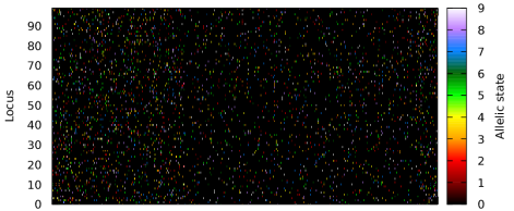
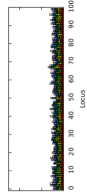
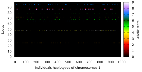
Figure 2: Haplotype heat maps of all chromosomes 1 found in an initial population of 250 women and 250 men. It presents 1000 haplotypes that correspond to the 1000 chromosomes 1 of the 500 diploid (initial) crew members. For each locus, a color code indicates its allelic state. The top figure shows the randomized population, in which 5% of variations (randomly distributed) are found within each genome, relative to the standard reference human genotype (all loci set to 0). The bottom figure shows a population for which individuals already share genetic patterns and whose genomes show an allelic variation of only 0.5% with respect to the standard reference human genotype (low diversity population). A stacked histogram on the right of each heat map allows to better visualize the distribution of the allelic forms for which the allelic state is non-zero (black alleles are not displayed for simplicity). Each bar represents the frequency of each allele with the same color code as in the heat map.

We programmed HERITAGE to automatically generate heat maps and stacked histograms representing the allelic composition (haplotype) of each chromosome, both at the beginning and at the end of the mission, together with graphs showing the degree of polymorphism P of the population, the heterozygosity index of individuals (I_k) and the heterozygosity index for each locus along chromosomes (H_i). In the rest of this publication, we will only show the results for chromosome 1 (for haplotypes heat maps and stacked histograms) for space saving purposes but all the chromosomes data are simultaneously plotted by the code.

In Fig. 2, we show on a heat map the 1000 different allelic patterns (haplotypes) of chromosomes 1 of an initial (zeroth) population of 500 individuals (250 males, 250 females). Since each of the 500 individuals is diploid (and has 2 chromosomes 1), 1000 chromosomes 1 are displayed. Allelic states found in the modeled loci are represented with a color code. We present the case of a randomized initial population (top figure, 5% of all loci carry variations) and the case of a non-random initial crew with much less allelic diversity (bottom figure, 0.5% variations). Both constitute extreme test cases that shall help present the possibilities offered by the improvements of the code to visualize changes in the allelic composition of traveling populations. Examples of non-random populations with variation levels of 5, 20 and 50% and pre-existing allelic patterns are also provided in Appendix B. In all cases, the initial population (500 individuals) is larger than the MVP thought to be needed for interstellar travel (100 individuals), such as determined in [11] to match more “classic” populations [36, 37, 38, 39].

In the case of a population with a randomized allelic diversity set to 5%, i.e. without previous genetic history or designed patterning, we see in the haplotypes heat maps and stacked histograms of Fig. 2 that most of the loci found on chromosome 1 have multiple allelic forms (polymorphism P is high), each with low and similar frequencies (within statistical fluctuations), which is characteristic of the random attribution of allelic states to loci. In the case of a low diversity population (allelic diversity set to 0.5%), the haplotypes heat map and stacked histogram show that allelic patterns do exist at the population level, which originates from pre-existing allelic patterns (haplotypes) implemented in ancestral populations. Also, only few allelic forms (1 to 3) in only a few loci (10 out of 100 on chromosome 1 in this example) exist (low polymorphism). Populations with variation levels of 5, 20 and 5080% were also tested (see Appendix B); as expected, polymorphism increases with variation levels, as well as the heterozygosity index of each locus (H_i), that reflects the increased allelic diversity, which translates into an increasing heterozygosity index at each locus (H_i) that describes the proportion of heterozygous individuals at those positions.

2.3 Gamete production, meiosis and formation of the n+1 generation

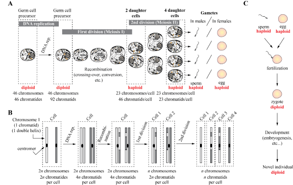
Figure 3: Principles of meiosis (formation of haploid egg and sperm cells from diploid precursor germ cells, panel A) and of genetic recombination followed by chromosomes and chromatids random shuffling (panel B). Panel C shows the formation a diploid individual from the haploid egg and sperm cells.

Once our initial population is created, we can run HERITAGE to generate the n+1 generation. A complete description of HERITAGE can be found in [10, 11, 12, 13], so we shall simply summarize the main steps for offspring’s generation. The code randomly selects two humans (one female and one male), checks that they are alive and within their procreation window, and determines by random draws if the two successfully mate. The code accounts for all necessary age-dependent biological parameters such as fertility, chances of pregnancy, miscarriage rate, etc. and checks whether the offspring is not inbred (within the security margins imposed by the user, using Wright’s genealogical parameters [14]). The new crew member is assigned an identification number. Various anthropometric parameters (weight, height, basal metabolic rate, etc.) are computed together with the life expectancy of the individual. Before the upgrades presented in this paper, we randomly assigned the sex of the offspring and did not account for her/his genetic heritage.

Now that each crew member of the zeroth-generation has a specific genotype, we can follow the rules of heredity to properly create the genotype of the offspring. The first step is to produce gametes (ova/eggs and spermatozoa/sperm, since only the variations present in these sexual cells are transmitted to the offspring). Gametes are produced from so-called germ line precursor cells, the only cells that can undergo meiosis. Meiosis is the process of double-cell division that allows switching from a diploid cell (two homologues for each chromosome) to four haploid cells (with a single chromosome of each kind in each cell, see [40, 41, 42] and Fig. 3 A). We recall that each human cell has 46 chromosomes that correspond to 22 (males) or 23 (females) homologous pairs. Chromosome 1 therefore exists in two homologous forms 1a and 1b, one (1b) from the father, the other (1a) from the mother. Their sequences are homologous, which means that they are similar but may carry sequence (state) differences, that is, they carry different haplotypes. It is the same for chromosomes 1 to 22 (1a, 1b, 2a, 2b, 3a, 3b …, 22a, 22b). This is different in the case of the sex chromosomes because female organisms have two homologous X chromosomes (Xa and Xb, from mother and father respectively), while males have one X chromosome (from the mother) and one Y chromosome (from the father) that are not homologous to each other.

During meiosis, the germ cells (cells that give rise to the gametes of an organism that reproduces sexually) start by duplicating all present DNA. This means that the 46 chromosomes present in the cell become duplicated. Chromosome 1a will therefore be duplicated in 1a and 1a’, the homologous chromosome 1b in 1b and 1b’, etc. Each chromosome therefore now possesses two chromatids (a and a’, b and b’, two DNA helices, clones of each other, see Fig. 3 B) which remain connected to each other by what is called the centromere. So, at this point, the amount of DNA is doubled, as it is the case for any cell division. Once everything is doubled, each pair of homologous chromosomes gets closer and both homologues undergo what is called homologous recombination (crossing-over event). In fact, one of the chromatids of one homologue interacts with one of the chromatids of the other homologue to form pairs of chromatids. There are four possible combinations: 1a with 1b, 1a with 1b’ or else 1a’ with 1b, or 1a’ with 1b’ (interactions of 1a with 1a’ or 1b with 1b’, although possible, are neglected, since they do not produce changes in allelic patterns/haplotypes). Only one of the combinations is chosen at random and the same is true for other chromosomes. These interactions occur over a certain lengths $l$ (the same on both chromatids). Homologous recombinations occurs within this interval. This means that the DNA sequences at these interaction zones make it possible to exchange the sequences contained in the interval of length $l$ between the two chromatids. For example, for the interaction of 1a with 1b, the exchange of sequences over a length $l$ between these two chromatids causes the passage of a segment from 1a to 1b, and reciprocally from 1b to 1a. It is the same for the other three combinations, if they are chosen. If the sequence exchange is unidirectional, that is, a sequence of length $l$ of chromatid 1a is shifted to chromatid 1b and replaces the original sequence, but reverse direction does not occur (1a remains unchanged), it is a phenomenon called conversion [41, 42]. By and large, the sequence contained in the interval $l$ of chromosome 1a imposes the sequence that will be present in 1b, but not the other way round. Overall, note that for any starting genotype constituted of two independent haplotypes, the homologous recombination and conversion (exchanges between homologous sequences) that takes place in germ cells will change the combination of alleles (haplotypes) found on individual chromosomes and randomly create genetic diversity, i.e. novel alleles combinations along chromosomes.

Once recombination and/or conversion are done, the homologous chromosomes are randomly separated and distributed in two different daughter cells. Therefore, each of the two daughter cells will contain 23 chromosomes with 2 chromatids each. The choice between 1a and 1b, 2a and 2b, etc. is entirely random, which, again, creates diversity. After this distribution, a second division of meiosis takes place for each of the two daughter cells. During this division, in each of the cells, the chromatids of each chromosome are separated and distributed in two daughter cells randomly. We thus obtain, from one starting germ cell, four daughter cells in total, each having 23 chromatids from the 46 starting chromosomes. These cells are haploid because they contain only one chromosome of each species and no longer two, as in the beginning. The process is the same for egg formation and sperm formation, so we do these genetic tasks for both the mother and the father (see Fig. 3 C). Homologous recombination, conversion, random separation of homologous chromosomes and random separation of chromatids shuffles the pre-existing genetic information, i.e. modify haplotypes of the final sexual cells (sperm or egg).

We must highlight the fact that the mechanism of meiosis, leading to four genetically different gametes, occurs for a single starting germ cell but there are thousands of germ cells, and millions of random possibilities of genetic shuffling in each one of them, so the combinatorics is really gigantic. This is why we use the full power of the Monte Carlo method to test all possible events and have a representative outcome of the meiosis. In HERITAGE, before mating, the code now uploads the vectors containing the mother’s and father’s genomes and creates haploid female (ovum/egg) and male (spermatozoon/sperm) gametes throughout the process described above. The algorithm performs recombination between pairs of homologous [X_ij] and [X’_ij] over intervals of length $l$ that are randomly selected between 3 $\leq l\leq$ 8 loci at the same time according to a discrete uniform distribution along the chromosome to make sure they do not always occur at the same place. In the code, there are 1 to 5 exchange areas per homologous pairs and the number of trades is also chosen at random. The code also allows conversion, i.e. the unidirectional exchange, over small areas (1 to 2 loci at maximum) with a known frequency of $\sim$ 10^-7 [43, 44, 45], so about 7.18 times over the entire genome in our simplified model of the human genome. For mating (and creation of a new individual), two final gametes, after meiosis, meet and pool their two haploid genomes to form a diploid genome containing two homologous chromosomes of each type. This genome is stored in a new vector of 2110 integers and is saved under the identification number of the child. The genome of the offspring is thus a novel combination of those haploid genomes from the two gametes, themselves selected from random but biologically-realistic processes. Pooling two Xs or one X and one Y makes it possible to determine the sex of the offspring in a sensible way, without imposing a ratio that, biologically speaking, does not actually exist since biological sex is due to this random pooling. Using this scheme, each novel individual resulting from the pooling of two haploid genomes from its parents’ sexual cells contains a novel and unique genotype, that is the result of the combination between two unique haplotypes obtained through meiosis in the parents.

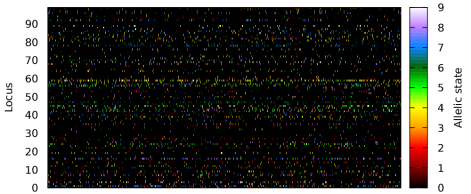
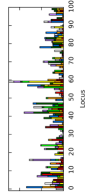
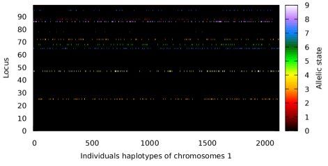
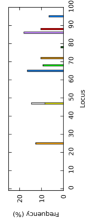
Figure 4: Haplotypes heat maps of all chromosomes 1 in a final population of approximately 1080 persons after 600 years of space travel under little-to-no cosmic ray radiation (no mutational effects). The top panel shows the genetic composition of a final population that descends from an initial randomized population in which the starting allelic diversity was 5%, with no pre-existing genetic patterns. Results (to be compared with Fig. 2, top panel) show that this final population, that is the result of a 600 year-long and complex genealogical history, now presents recognizable allelic patterns that are visible on the heat map and highlighted by significant changes in the number and frequencies of alleles for discrete loci. The bottom panel shows the genetic composition of a final population that descends from an initial low diversity population in which the starting allelic diversity was 0.5%, with pre-existing genetic patterns. Results (to be compared with Fig. 2, bottom panel) show that allelic patterns did not change significantly, but that allelic frequencies changed.

Fig. 4 presents the results of 600 years of breeding for the enclosed population in the spaceship, following the newly implemented biological laws. The ship’s volume capacity was fixed to 1200 inhabitants at maximum, with a security threshold of 90% to avoid overpopulation. Consanguinity was not allowed (up to first cousins once removed or half-first cousins, i.e., a consanguinity factor of 3.125% or below) in this simulation. The procreation window was selected to be between 30 and 40 years old according to the results from our previous publications [11, 12]. The top panel shows the genetic composition of a final population that descends from an initial randomized population in which the starting allelic diversity was 5%, with no pre-existing genetic patterns (random assignment of allelic states for  5% of loci). This final population is the result of a 600 year-long and complex genealogical history that produced novel genotypes through meiosis (genetic recombination, chromosomes and chromatids random shuffling) and random mating. The results (to be compared with Fig. 2, top panel) show that, contrary to the initial population, recognizable allelic patterns are now visible on the heat map of the final population. This is also highlighted by significant changes in the number and frequencies of alleles of discrete loci. Several alleles have been favored – others eliminated – by crossing-over, conversion and mating histories and the global genetic diversity of the final population shows clear differences with respect to the completely randomized distribution from year 0. While our theoretical population is not realistic (no pre-existing patterns), the results highlight the fact that the biological laws we have implemented work well and can generate novel allelic patterns that are the result of genetic recombination and shuffling mechanisms (see also Appendix A). The genetic diversity of the final population is still close to the initial value of 5% since neomutations were not permitted. This denotes that the number of starting individuals was enough, and that this number remained enough to stabilize allelic diversity, as if the population approached the Hardy-Weinberg equilibrium. The bottom heat map and stacked histogram show the genetic composition of a final population that descends from an initial low diversity population in which the starting allelic diversity was 0.5%, with pre-existing genetic patterns. Results (to be compared with Fig. 2, bottom panel) highlight that allelic patterns did not change significantly, but that allelic frequencies did. This comes from the fact that the starting allelic patterns and allelic diversity were highly reduced, which decreased the combinatorics possibilities, contrary to the above-mentioned randomized population. However, we observe stochastic changes in allele frequencies: some alleles are much less present than in the beginning of the journey, while some others have increased. This illustrates the genetic drift that resulted in changes in allelic frequencies from sampling effects (mating, recombination, etc.) in small populations. Genetic drift promotes intergroup differentiation in the long term. Here, the final genetic diversity is close to the initial one due to the absence of spontaneous or cosmic-ray induced mutations.

2.4 Introducing mutations

The stability of the genetic information is central to the normal function of cells and, more importantly to the reproduction of living organisms. It is therefore of vital importance to maintain genomic stability within the somatic (non-sexual) cells that constitute all the organs, tissues and structures of the body. Genomic stability avoid deleterious alterations of homeostasis and proliferation that could cause, among others, carcinogenesis, but also in sexual (germ line) cells that ensure transmission of this information to the offspring. This stability is ensured in both types of cells by the enzymatic (protein) machineries that replicate DNA [46] and by those that correct inevitable replication errors (mutations [47, 48]), a balance that results in very low mutation rates [49]. Mutations are modifications of DNA sequences. They naturally and continuously occur within cells as a result of physicochemical constraints imposed to DNA itself but also to the cellular machineries and processes that ensure DNA replication and transmission [50]. When they arise in germ cells, they are the cause of changes in the genetic composition of the offspring that are responsible for the emergence of novel polymorphisms (sequence variants), i.e. alleles, that make individuals genetically different (in addition to the genetic recombination and shuffling due to meiosis).

When a cell divides (mitosis), it must duplicate its entire genome and DNA polymerases are the enzymes (proteins) that catalyze the synthesis (polymerization) of a novel DNA strand using a single stranded DNA template, free nucleotides and the “complementarity rules” [46]. They possess “proofreading” activities that ensure correction of several types of errors, such as mismatches (wrong base-pairings), during or after replication [46, 51]. Oxidative, chemical or radiation-induced stress can alter the nucleotides chemistry, thereby influencing their base-pairing properties and leading to mismatches that lead to so-called punctual mutations. These stresses can also provoke various types of covalent cross-links between nucleotides and/or strands, as well as DNA single or double strand breaks that all alter the integrity of the genetic information and perturbs faithful DNA replication. This can lead to small or large sequence deletions (losses), insertions or duplications [52, 53, 54]. Those novel mutations (neo-mutations) may have deleterious effects [55]. Sometimes, alterations lead to large scale chromosomal rearrangements, i.e. changes in the architecture of chromosomes (whole region duplications, deletions, translocation of sequence elements from one chromosome to the other, fusions of chromosomes, etc.) that can all affect the overall physiology or even survival of cells [56]. Moreover, chemicals- or radiation-induced stress can dramatically increase abnormal chromosome and/or chromatids segregation during mitosis (cell division) or meiosis (germ cells’ specialized division, see above), leading to erroneous partition of the genetic material and of chromosomes, inducing aneuploidies (wrong number of chromosomes in one cell) that are highly detrimental to somatic cells [57] or to reproduction when they occur in sexual cells [58, 59].

However, cells are equipped with DNA repair proteins that detect and resolve mismatches and other types of DNA alteration, such as nucleotides chemical alterations, strands breaks, etc. triggered by oxidative-, chemical- or radiation-induced stresses [50, 52, 53, 54, 48]. Overall, DNA polymerase proofreading activities and DNA repair processes keep mutation rates very low, in the order of 1 erroneous nucleotide incorporated every 10⁸ to 10¹⁰ added nucleotide during replication [47, 46, 51]. As a result, the mutation rate is on the order of 10^-8 single nucleotide mutation per base pair per generation in germ line cells in humans (depending on the age of the individual), while small deletions or insertions are on the order of $\sim$ 10^-9. Duplication or deletion of regions of 50 bp or more occur at rates of $\sim$ 10^-4 – 10^-2, depending on the sequence’s length [49]. Despite those frequencies, punctual mutations (single nucleotide variants) and small deletions/insertions are, by far, the most frequent, likely because large scale changes (deletions, insertions or displacement of larger sequences) are deleterious and cannot be transmitted to or by the offspring [49].

Let, again, “A” be the first chromosome. We have [A_i]=(A₁, A₂, A₃, A₄ … A_n) the set of loci indexed in the order of localization along A. Let [A${}_{i}j$] be the chromosome A containing $n$ loci for which each can take the state $j$, that varies from 0, the “reference state”, to $m$, with, in our case $m$ taking one single value on one haplotype, comprised between 0 and 9 (only 10 different alleles of a given locus are authorized to exist in the initial population). If a mutation occurs in germ line cells inside one of these loci, then its state $j$ takes an integer value $k$ that, by definition, has to be different from the other pre-existing values (for other allelic forms). In reality, a mutation could, in principle, change the allelic state of one allele to a state that is identical to another, already existing allele, within the population. However, given the size (in bp) associated to each locus, such mutations are highly improbable and shall be neglected. We take a mutation rate (that is also the mutation probability) of 1.2 $\times$ 10^-8 single nucleotide change per base pair per generation [49]. For simplicity, all de novo mutations shall account for punctual mutations or small deletions/insertions. Larger DNA rearrangements, such as large scale deletions/insertions or even gene duplications, chromosomal changes (translocations, fusions, etc.) will not be considered in this work

2.5 Impact of cosmic rays

In the interstellar medium, a continuous flux of atomic nuclei and high energy (relativistic) particles have been detected [60, 61]. These cosmic radiation consist mainly of charged particles [62, 63, 64]: protons (88%), helium nuclei (9%), antiprotons, electrons, positrons and neutral particles (gamma rays, neutrinos and neutrons). The sources of the most energetic radiation (whose energy exceeds 10²⁰ eV) are not yet fully identified but are likely to be extra-galactic in nature (either from active galactic nuclei or the collapse of super-massive stars [65]). These particles are extremely harmful to Earth-like life [66] because they carry enough energy to ionize or remove electrons from atoms, possibly leading to DNA breaks and/or alterations [67].

Radiation (heavy ions, ionizing radiations, etc.) can induce chemical group modifications on nucleotides and change their base-paring properties, but also produce cross-links between nucleotides, and/or induce DNA single- or double-strand beaks [68, 52, 53, 54]. These alterations may be repaired by the DNA repair machineries [53, 48]. However, space conditions such as microgravity and/or radiation can cause DNA damage and affect DNA repair mechanisms to the extent that genetic mutations may accumulate over time, especially in somatic (non-sexual) cells [69]. Somatic cells in the human body (or any embarked animal or plant) would be the main victims of such radiation, with effects that depend on the type of radiations and localization and properties of affected tissues. DNA alterations caused by space radiation are not necessarily repaired [69] by the dedicated cellular machineries [52, 54], which can perturb DNA replication and cause genomic instability [70], thereby leading to mutations of various possible types in somatic cells that may produce detrimental effects such as cellular deregulations, cell death and cancers (carcinogenesis) [71, 72, 73, 74, 75]. These may also be the cause of various health issues and pathologies [76, 77, 78], including nervous system alterations [79, 80]. Such somatic cell DNA alterations would not be transmitted to the offspring. If occurring in exposed embryos or fetuses [81, 82], they could also trigger developmental deregulations, malformations or cancers.

Of course, if genetic alterations caused by space radiation occur in germ line (sexual) cells, they are, only in this case – if not repaired –, transmitted to the offspring [83], potentially leading to congenital diseases and/or other abnormalities [76, 77, 84], if the associated mutations are not neutral. Studies on mouse models show that mutation rates increase in germ line cells when they are chronically exposed to ionizing radiations, especially in males, and that the effect becomes much greater for acute exposures and the same can likely be extended to humans [83, 85]. Fortunately some of the space radiation and high energy particles are deflected by the solar wind and, at ground level on Earth, they are widely dispersed by the magnetosphere or blocked by the atmosphere and its particles in suspension. Because of this, cosmic radiation only accounts for 13 to 15% of terrestrial radioactivity [86]. However, in space, the annual flux of cosmic radiation received by astronauts is greater and therefore represents a danger [66]. This danger is all the greater as one moves away from the Sun and its natural protection. It is therefore understandable that cosmic radiation (and its impact on the human genome and overall health) is a considerable risk for any interstellar travel.

(a) Constant annual radiation dose: 0.3 mSv.

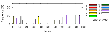
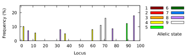
(b) Constant annual radiation dose: 3 mSv.

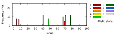
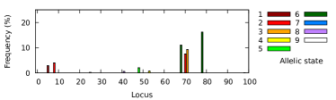
(c) Constant annual radiation dose: 30 mSv.

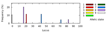
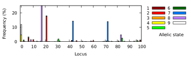
(d) Constant annual radiation dose: 300 mSv.

Figure 5: Effect of radiation on the overall allelic composition. Stacked histograms show the frequency of alleles found on chromosomes 1 for an initial, gender-balanced, “low diversity” population of 500 crew members (left figures) and for the final final populations of approximately 1080 persons after 600 years of space travel (right figures). Each row corresponds to a different constant annual radiation dose: 0.3, 3, 30 and 300 mSv.

For this reason, we decided to take into account radiation-induced mutations in our recent upgrades of HERITAGE. To do so, we allow the user to fix an annual equivalent dose of cosmic ray radiation (in milli-Sieverts) at the beginning of the simulation. This represents the effectiveness of cosmic ray shielding of the spacecraft. This value can be changed during the interstellar travel to simulate the degradation of the shielding material/technology, but also to mimic a nuclear disaster from, e.g., the propulsion system or a nearby and unexpected supernova event. In the framework of the Earth’s magnetosphere and atmospheric protection, the annual dose of radiation is of the order of 0.3 – 4.0 mSv in European countries [87]. This corresponds to a mutation rate that is less or equal than 10^-3 per generation per individual [88], much more than the estimated  10^-8 [49] under normal terrestrial conditions. We thus include in our simulation an additional random draw that is compared to the mutation rate scaled with respect to the annual dose of radiation, so that larger cosmic ray doses imply larger mutation rates. Note, however, that this is a simplification since the mutation rate as a function of cosmic ray impacts in deep space is yet to be measured and understood. The number of loci randomly affected by mutations is determined by the combination of the annual radiation dose and the mutation rate. In the case of 0.3 mSv per year, less than one locus is affected per generation per individual. In our model, any mutation of any kind that occurs within a locus $i$ that has a state $j$ shall be indicated by a change in the value of $j$, with the only restriction that the value must be different from those already present.

We ran HERITAGE for four different initial populations of 250 women and 250 men with a pre-existing genetic history (the “low diversity” population option). The space travel duration was set to 600 years. The ship’s maximum capacity, overpopulation threshold and authorized consanguinity are similar to those simulated in Sect. 2.3. With all the new biological upgrades, the codes now takes 3.6 times longer to complete. A single-run simulation (no iterations of the same trip) is achieved in 22 seconds using the input parameters described above. In Fig. 5, we present the effects of neomutations on the human genome after 600 years of space travel with four different constant annual radiation dose: 0.3, 3, 30 and 300 mSv. The first and second doses correspond to the annual background radiation on Earth at sea level and in US countries [89]. The third dose is representative of about 3 months on-board of the International Space Station [90] and the fourth dose to about 500 days on Mars [91]. Beyond the effects of genetic drift – that can change the frequency of pre-existing alleles –, we can see that mutations are very rare within 600 years for radiation doses of 0.3 and 3 mSv. The mutations either did not affect the genome, or were randomly lost during genetic recombination and chromosome shuffling (meiosis) or from biased sampling during mating. Very low-frequency neomutations emerged in the case of an annual radiation dose of 30 mSv and are still visible after 600 years. On average, they are well below the frequencies of the alleles that were initially present in the starting population. When considering an annual dose of 300 mSv, neomutations become more populated, impacting the genetic composition of the final population in a more substantial fashion, although novel alleles remain low-frequency variations.

Again, note that, like for allele combinations, neomutations that change the genotypes found in and transmitted by individuals are all neutral, with no deleterious (negative) or advantageous (positive) effects. Therefore, they do not affect the offspring (diseases, reduced life expectancy, etc.) or the probability that descendants can reproduce (sterility, fertility, etc.). All mutations that become transmitted after genetic recombination, chromosome shuffling (meiosis) and random mating therefore remain present in the population’s genetic pool, unless they are randomly lost according to the same genetic (meiosis) and reproductive (mating) mechanisms. Of note, those mutations that become transmitted to the offspring originate from changes in the haploid genomes of germ cells. However, we must remind that mutations also accumulate in somatic (non-sexual) cells of individuals during and as a function of their lifetime. This, in reality, would likely lead to cancers or other physiological perturbations, a fact that we do not take into account and that could also influence the transmission of germ cell-specific mutations, in addition to the effect of mutations acquired from ancestors. At high doses (300 mSv), individuals in the population could therefore be strongly affected by mutation-induced pathologies that affect the soma (e.g. cancers), i.e. somatic cells, which could change life expectancy, health, fertility, etc. in the whole population. Germ cells-specific mutations can be transmitted to the offspring and affect children with genetic diseases that can themselves change life expectancy, health, fertility, and even the capacity of cells to repair radiation-induced DNA alterations (increased mutational rate). This would most likely strongly and durably affect the entire population, with a time-dependent and cumulative worsening that could eventually completely wipe out the crew. It is interesting to note that our simulations demonstrate that at levels superior to 30 mSv, the human genome suffers numerous genetic changes (at the population and generation scales) that could be fatal, which is in perfect agreement with the regulatory dose limits of radiation workers (50 mSv) defined by federal (i.e., the Environmental Protection Agency – EPA –, the Nuclear Regulatory Commission – NRC – and the Department of Energy – DOE –) and state agencies (e.g., Agreement States) to limit cancer risk.

3 Genetic effects over 600 years of interstellar travel

3.1 Demographic results

Now that HERITAGE is able to compute, manipulate and store genetic data, we decided to run it in the context of a 600 years space travel towards any interesting target. For continuity purposes, we kept the same HERITAGE parametrization as before (250 women and 250 men for the first generation, consanguinity factor below 3%, etc.) and concentrate on the analysis of the population demographics. We simulate a catastrophic event at year 350 that will wipe out 30% of the population chosen at random. This will allow us to see the effect of a so-called “bottleneck event” (that affects the genetic composition of a population without selective effects on genes, i.e. rapid catastrophic events) in addition to genetic drift and mutations on the global genetic (allelic) composition of the final deme. We consider a state-of-the-art radiation shield so that the annual equivalent dose of cosmic ray radiation is similar to the Earth radioactivity background at sea level (0.3 mSv). The initial crew is young (20 years on average), carefully picked from five different existing populations (the “low diversity” option) but without family connexions at this point. We use the adaptive social engineering principles established in our series of publications [10, 11]: each woman can have 3 $\pm$ 1 children over the course of her life but if overpopulation onsets the code will reduce this value so that there will be internal population regulation. In comparison with our previous calculations, we decreased the standard deviation of the female and male life expectancy (from 15 to 5) in order to better mirror current reality [92, 93]. We also extended the procreation period from 30 – 40 years to 18 – 40 years in order to mitigate the sibships effect [94]. To calculate the total energy expenditure of the crew per year, we consider that the population is vigorously active between age 20 – 45 and less active before and after. We will loop HERITAGE over one hundred iterations since this is enough for reasonable demographic estimates [95, 12]. However, we must note that each iteration of the code will now produce different initial population genetics. This will become useful for determining the slow changes in the genetics of the crew throughout the space travel. Tab. 2 lists all the parameters that we fixed before starting the simulation. Extensive explication, details and description of the parameters are given in [10, 11, 12, 13].

Parameters	Values	Units
Number of space voyages to simulate	100	–
Duration of the interstellar travel	600	years
Colony ship capacity	1200	humans
Overpopulation threshold	0.9	fraction
Inclusion of Adaptive Social Engineering Principles (0 = no, 1 = yes)	1	–
Genetically realistic initial population (0 = no, 1 = yes)	1	–
Number of initial women	250	humans
Number of initial men	250	humans
Age of the initial women	20 $\pm$ 1	years
Age of the initial men	20 $\pm$ 1	years
Number of children per woman	3 $\pm$ 1	humans
Twinning rate	0.015	fraction
Life expectancy for women	85 $\pm$ 5	years
Life expectancy for men	79 $\pm$ 5	years
Mean age of menopause	45	years
Start of permitted procreation	18	years
End of permitted procreation	40	years
Initial consanguinity	0	fraction
Allowed consanguinity	0	fraction
Life reduction due to consanguinity	0.5	fraction
Possibility of a catastrophic event (0 = no, 1 = yes)	1	–
Fraction of the crew affected by the catastrophe	0.3	fraction
Year at which the disaster will happen (year; 0 = random)	350	years
Chaotic element of any human expedition	0.001	fraction

Table 2: Input parameters of the simulation. The $\mu$ $\pm$ $\sigma$ values shown for certain parameters indicate that the code needs a mean ($\mu$) and a standard deviation value ($\sigma$) to sample a number from of a normal (Gaussian) distribution.

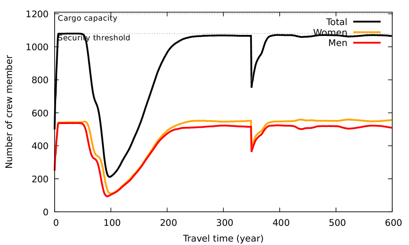
(a) Crew evolution in terms of population number (orange: women, red: men, black: total).

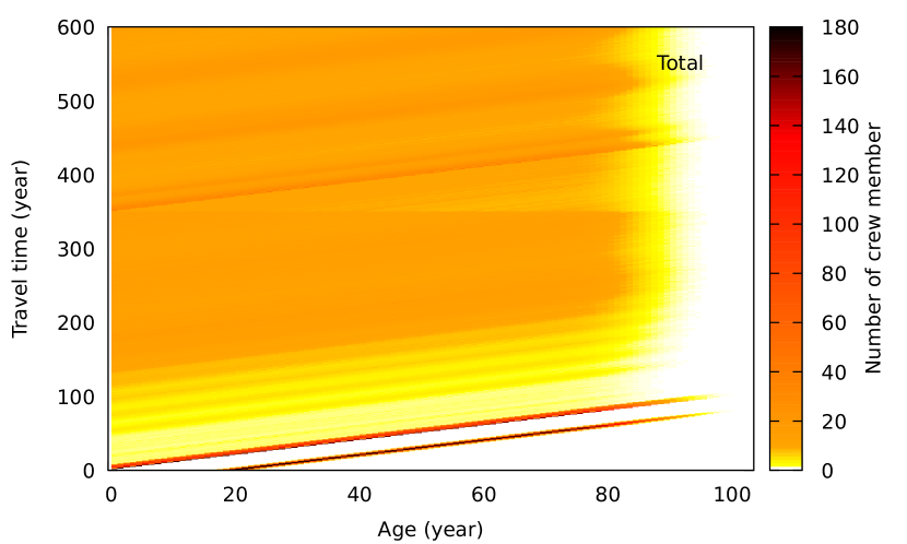
(b) Density of crew members of a given age (x-axis) over time (y-axis). The population density is color-coded from 0 (white) to maximum (black).

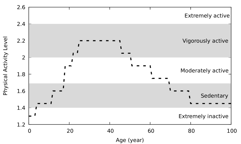
(c) Physical activity level (PAL) scenario for our population model.

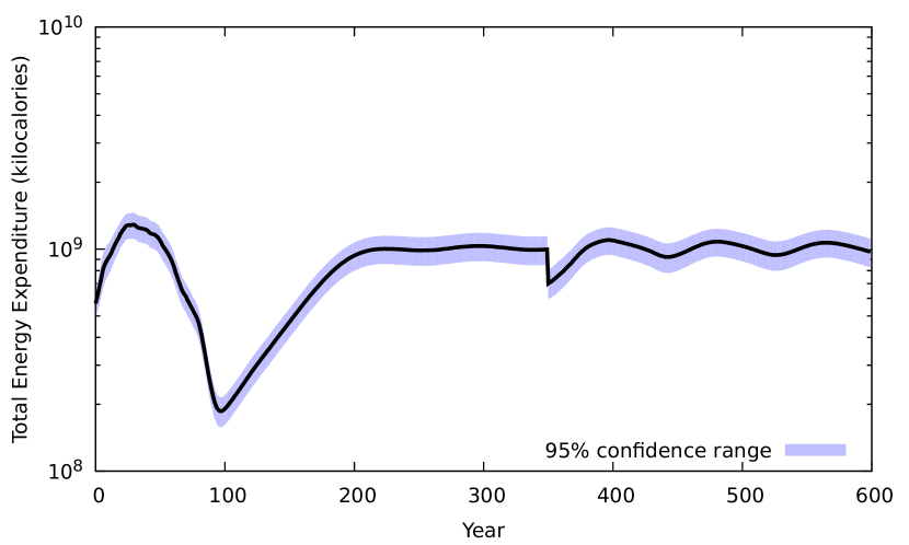
(d) Total energy expenditure (TEE, in kilo-calories) per year in the vessel for the considered PAL scenario.

Figure 6: HERITAGE results for a 600 years-long interstellar travel under the conditions described in the text.

In Fig. 6, we present the outcomes of the simulation in terms of demography and food consumption on-board. We can see that the population quickly heads towards the overpopulation threshold in two generations. The adaptive social engineering principles activate and we see a decrease of the population demography before a slower, second increase that would ultimately lead to stabilization except for the presence of the catastrophe at year 350. The strong demographical decrease at year $\sim$ 50 is due to the presence of sibships within the spacecraft: the zeroth-generation being very young, its results in well-defined demographic echelons during the first 200 years such as seen from Fig. 6 (b). Those demographic echelons, predicted by Moore [94], are impacting at the beginning of the travel until the various generation clusters mix in age. We also note that the minor demographic changes compared to the previous papers have not had a significant change on the end results. The physical activity level scenario in our simulation (Fig. 6, c) drives a total energy expenditure of approximately 10⁹ kilo-calories per year in the vessel (Fig. 6, d). From a demographic and metabolic point-of-view, the crew seems perfectly fine at the end of the mission.

3.2 Genetic results

3.2.1 The Hardy-Weinberg equilibrium

How to verify the genetic health of the multi-generational crew? The first test to be carried out is whether the population is at the Hardy-Weinberg (HW) equilibrium when there are no mutations [36, 37]: for a sufficiently large population (ideally infinite), the frequency of alleles (for non-sexual chromosomes) should tend to be stable over long periods (in our case $>$ 600 years). If the frequencies stay almost constant, this would confirm that the initial genetic diversity is likely to remain more or less constant (the population remains genetically varied like the original one). This means that the number of breeding individuals is sufficient to ensure a constant mixing of genes. This verification makes it possible to say that, if there are no mutations (and therefore no increase in potential genetic variability), the population is likely to be genetically stable. This is the first test geneticists would use before a multi-generational trip to probe the potential stability of the population.

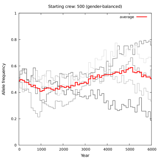
Figure 7: Results of genetic drift on the frequency of an allele at a randomly-chosen locus (that has two allelic forms) in a randomly-chosen chromosome. The changes in frequency is followed at every generation from the initial population presented in Tab. 2. The five gray lines represent the frequency of an allele in 5 independent populations while the thick red line represents the average frequency. The simulation was extended to 6 000 years in order to see any long-term effect on the genetic stability of the populations. The initial population consists of 500 gender-balanced individuals.

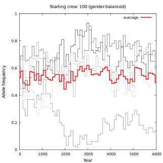
Figure 8: Same as in Fig. 7 but for an initial crew of 100 gender-balanced persons. This smaller population allows us to visualize the effects of the starting population’s size on the genetic drift.

In Fig. 7, we explored the allele frequency variations inside the multi-generational population with a departing crew of 500. To do so, we artificially imposed the frequency of the alleles at a random locus along the genome to be randomly but equally distributed between integer values 0 and 1. In other words, a randomly chosen locus is assigned two possible alleles with frequencies of 0.5 (50%) each. This is an idealized and simplified situation that facilitates the visualization of the genetic drift on the frequency of one of both alleles to determine whether this specific locus follows the Hardy-Weinberg equilibrium (stable frequency of alleles over time). We then ran HERITAGE and increased the duration of the interstellar travel from 600 to 6 000 years to check whether dramatic allele frequency variations could happen after the nominal period of 600 years. For the initial crew described in the previous section, we find that the average of numerous (repeated) simulations tends to show a nearly-constant frequency around 50%, indicative of the fact that the frequency of the allele under inspection remains stable over time, i.e. is nearly at the Hardy-Weinberg equilibrium, which is what one would expect for a population of more than 50 people [96]. The differences are simply due to the fact that we do not necessarily have clearly separated generations, and that the individuals are not all synchronous (in births, in age, in reproduction timing, etc.) contrary to theoretical models [97]. From these deviations from HW conditions, small stochastic variations of allelic frequencies occur even in the case of a population theoretically composed of enough individuals (more than 50 reproducing individuals). For a smaller population (Fig. 8), sampling bias and deviations from the theoretical HW conditions more strongly affect allele frequencies. The averaged frequency does also oscillate around 50% but stochastic variations are much larger. Yet, the population is close to the Hardy-Weinberg equilibrium, although it is more easily affected by sampling bias, which means that the HW equilibrium is more easily lost with a smaller population and that larger populations are better at avoiding this. This was already expected from previous findings [96], from results obtained by monitoring the heterozygosity index (see above) and it advantageously confirms the conclusions of our previous publication, in which we stated that at least 98 people should constitute the zeroth-generation crew of any multi-generational mission [11]. Our first preliminary tests, applied to one bi-allelic locus, indicate that our multi-generational population would likely be genetically healthy, in the sense that 100 to 500 people would be enough to stabilize allele frequencies and, consequently, the starting genetic diversity, at least over a 6 000 year-long period of time. Of course, now that we have implemented virtual genomes that carry thousands of loci with multiple possible allelic forms, we will be able to extend this analysis (HW equilibrium, frequency variations, etc.) at the genome-scale with more appropriate tools as we did by measuring polymorphism, heterozygosity indices and consanguinity.

3.2.2 Nei’s minimum genetic distance

Now that we have confirmed that the allele frequencies in the crew are likely stable in the long run, it is necessary to determine the impact of time (i.e. genetic recombination and shuffling during meiosis, matings, etc.) on the genetic composition of the crew in comparison to the zeroth-generation. To do so, we can compute the genetic distance $D_{\rm A}$ that measures the degree of differentiation: populations with many similar alleles have small genetic distances (they share similar genotypes, i.e. allelic patterns and are closer to a “common ancestor” population) while populations with more different allelic patterns or genotypes are separated by greater genetic distances. To determine the genetic distance, we used the Nei’s minimum genetic distance [98] that assumes that genetic differences arise mainly from mutation and genetic drift (which is the case here):

$$\textsl{{D}}_{\rm A}=1-\sum_{l}\sum_{u}\sqrt{X_{u}Y_{u}}/L,$$

where $X$ and $Y$ represent two different populations for which $L$ loci have been studied. In our calculus, $X$ is the zeroth-generation while $Y$ is the population after a given time. $X_{u}$ and $Y_{u}$ represent the $u^{th}$ allele frequencies at the $l^{th}$ locus. $D_{\rm A}$ = 0 means that the n^th generation is identical to the zeroth-generation and with increasing $D_{\rm A}$’s the genome of the population starts to differ from the initial one. A Nei’s minimum genetic distance between 0 and 0.05% indicates that the initial and final populations are very similar (in the sense that they share very similar allelic patterns) and likely poorly differentiated [99]. A value between 0.02 and 0.2% usually indicates that two (or more) populations are likely subspecies (e.g., the Bengal and Siberian tigers are examples of subspecies), which should be understood as “populations with sufficiently different allelic/genetic patterns to arbitrarily subdivise them into distinct entities” [99]. Values between 0.1 and 2% usually imply that the two (or more) populations under investigation are different species (e.g., cats, chickens and chimpanzees are three examples of species) [99]. Here, the term “species” must be considered carefully. In general, individuals or populations are considered to belong to the same species if they can breed and produce descendants that are themselves inter-fertile. However, in an evolutionary point-of-view, the concept of species arbitrarily encompasses all individuals that belong to a continuous genealogical flow/continuum (meaning that time is also part of the definition). All groups of individuals (populations) that have, though, similar genetic features but that do not (or not anymore) contribute to this genealogical flow (infertility, incompatibility of gametes, etc.), and that are part of a sister, but separated genealogical flow, are considered other species, by definition. Speciation is therefore not a discrete event, since the assignment of individuals to a particular group is arbitrary. However, the emergence of reproductive and/or biological incompatibilities (genetic reproductive barriers, etc.) constitutes the origin of separated genetic lineages that we name species [100]. The amount of genetic differences required to reproductively isolate populations from each other is not known and depends on incalculable possible combinations of genetic (mutational, genotypic, etc.), phenotypic (including behavioral) and environmental effects. For this reason, and because we did not (and cannot) model the tremendously complex mechanisms that drive reproductive compatibility, or influence reproductive isolation in the case of isolated human populations traveling through space for generations, the evaluation of the genetic distance (following Nei) will not be used to speculate on the emergence of human subspecies or species.

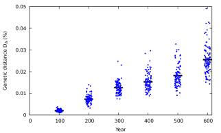
Figure 9: Evolution of the Nei’s minimum genetic distance $D_{\rm A}$ as a function of time for the HERITAGE parametrization presented in Fig. 6. Each point (at a given time-step) represents the outcome of one out of one hundred simulations. The averaged genetic distance is highlighted by a black bar. The annual equivalent dose of cosmic ray radiation is similar to the Earth radioactivity background at sea level (0.3 mSv).

We plot in Fig. 9 the time-dependent evolution of the genetic distance between the zeroth and the n^th generations (with 100 years steps). Each point (at a given time-step) represents the outcome of one out of one hundred simulations. The averaged genetic distance $D_{\rm A}$ is highlighted by a black bar. We can see a large spread around the mean that is predominantly due to the effect of genetic drift, that can change allelic patterns (haplotypes, genotypes). The increase in genetic distance is somewhat linear with time if we consider the mean values (such as expected from [99]) but we also observe that the tail of the $D_{\rm A}$ distribution is quite large. This means that the outcomes of 600 years of space travel most often lead to genetically not-so-different populations with respect to their zeroth-generation. This is in agreement with the results presented above, from which we concluded that our traveling populations are close to the HW equilibrium, a state that ensures the stabilization of alleles within populations. Consequently, under the neutral hypothesis condition we used (no phenotypic effect of mutations, allelic patterns, etc.), no natural selection of alleles or allelic patterns (haplotypes or genotypes) are expected, which reduces the otherwise unavoidable genetic differentiation of the population, with respect to the initial one (or to the one that remained on Earth). Yet, the genetic distance increases with time, because the deviations from the Hardy-Weinberg conditions, although small, tend to have cumulative effects that eventually affect the genetic composition of populations. Genetic differentiation, as expected, is unavoidable, because the genetic input within the vessel is limited, subjected to genetic drift with potential losses of alleles, and there is no external genetic input (from other human populations) that could replenish the genetic pool with primitive (original) alleles that could reconstitute the starting allelic diversity. Some extreme cases ($D_{\rm A}\approx$ 0.05%) may appear from those purely stochastic sampling effects (recombination, chromosome shuffling, mating), leading to genetically different sub-groups on-board (with respect to the 0^th generation). The distribution of the Nei’s minimum genetic distance at the 600 year time-step is illustrated in Fig. 10. It is a positively skewed unimodal distribution (the tail is on the right of the histogram) that originates from the relative small size of the populations but also from genetic drift. In some rare and extreme cases, several allele frequencies can drastically change, affecting the allelic composition, leading to larger genetic distances. Note that genetic differentiation occurs on-board during the journey, and that is will continue after arrival. As mentioned, measuring the Nei’s distance does not tell anything on the speciation of interstellar populations, but certainly illustrates that genetic differentiation will occur at rates that depend on the genetic drift and on the populations’ size.

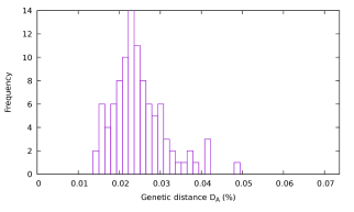
Figure 10: Histogram of the Nei’s minimum genetic distance between the final 100 populations and their respective zeroth-generation genome after 600 years of interstellar travel with low cosmic ray radiation (0.3 mSv).

For a purely scholastic experience, we can run one hundred more simulations with a much higher annual equivalent dose of cosmic ray radiation (300 mSv). While the crew would likely be wiped out by cancers and genetic disorders first, we can observe in Figs. 11 and 12 the effects of neutral mutations onto the Nei’s genetic distance after 600 years under those extreme conditions. In Fig. 11 we see that speciation (in the sense of Nei) or, more properly formulated, “strong genetic differentiation” would occur relatively quickly ($\geq$ 300 years) but also that the spread in genetic distances between the one hundred different populations is not so large. This is due to the fact that genetic drift becomes less important than the accumulation (at high rates) of spontaneous mutations. This latter phenomenon is unlikely to occur in reality, due to selection effects that would filter out numerous mutations or allelic combinations, reducing the differentiation rate accordingly. The histogram of $D_{\rm A}$ at year 600 (Fig. 12) is still a positively skewed unimodal distribution but the skewness factor is less prominent than in the case of negligible radiation doses.

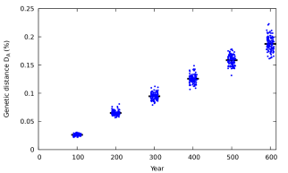
Figure 11: Same as Fig. 9 but with a higher annual equivalent dose of cosmic ray radiation (300 mSv).

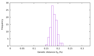
Figure 12: Same as Fig. 10 but with a higher annual equivalent dose of cosmic ray radiation (300 mSv).

4 Conclusions and further development

We have significantly upgraded the agent based Monte Carlo code HERITAGE in order to include a representative toy model of the human genome for each crew member. We implemented biologically realistic gamete production processes (meiosis), including crossing-over, unilateral conversion, chromosomes and chromatids shuffling, etc. Those new implementations allow us to perform genetic simulations on multi-generational populations in a large parameter phase space. We can now determine if, from an initial population of a given size and with a defined genetic composition, it would be possible to preserve sufficient allelic diversity over time and test the contribution of neomutations from cosmic ray radiation.

In this work, we assumed that all combinations of alleles (genotypes) and mutations have neutral phenotypic effects (neutral hypothesis). In this case, and using a single bi-allelic locus as a probe (as in [15]), we found that a MVP of about 100 gender-balanced people at the beginning of the interstellar travel would likely be close to the Hardy-Weinberg equilibrium (during the course of a 6000 years journey), which is expected to preserve most of the genetic diversity selected for the initial crew. This initial crew can also sustain genetic drift and small amounts of (neutral) neomutations, and arrive “genetically healthy” at the end of 600 years of deep space travel with state-of-the-art radiation shields. However, we observed that the Hardy-Weinberg equilibrium can easily be lost, and that its stabilization effect suppressed in the case of stronger radiation fluxes or catastrophic demographic events. It results that a safer and more adapted population threshold should be considered, probably in the range of a few hundred individuals. We indeed have experimented our code with a MVP of 500 crew members and found it more resilient. Nevertheless, it is too soon to conclude yet since we must exploit the full potential of our code to analyze genetic effects (HW equilibrium as a function of the number of crew members and allelic diversity) at the genomic (multi-locus) scale. We also have to move away from the neutral hypothesis and include phenotypic effects of allelic combinations, and more importantly, of neo-mutations, since this is likely to strongly influence the evolution of the genetic composition and structure of populations. Indeed, as discussed above, allelic combinations, mutations and interactions with the environment (external or internal, i.e. biological, cellular, etc.) can lead to selective effects (positive, negative or neutral effects). This will be achieved in the second part of this paper series. To take into account these complex effects, we will rely on the extended literature on population genetics of mutations [101, 102, 103]. It is highly probable that strong annual doses of radiation will most likely wipe out the interstellar crew rather than lead to strong differentiation in a time-frame of a few hundred years. However, we will be able to check the impact of any nuclear accident inside the spacecraft by artificially increasing the annual dose of radiation to a maximum peak for only a year, before returning to safer doses. In turn, we will have access to realistic simulations for managing nuclear accidents on Earth, such as the Chernobyl catastrophe [104, 105, 106] or the more recent triple nuclear meltdown in Fukushima Dai-ichi [107, 108].

APPENDIX A: Validating the numerical biological laws in the code

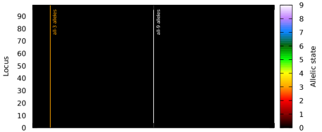
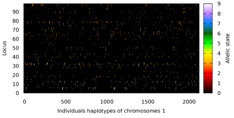
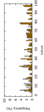
Figure 13: Haplotypes heat maps of all chromosomes 1 in an initial and final population after 600 years of space travel under little-to-no cosmic ray radiation (no mutational effects). The top panel shows the genetic composition of an initial theoretical population that is homozygous at all positions. All allelic states are set to 0, except for two individuals (“all-3 genotype” and “all-9 genotype”). The bottom panel shows the allelic patterns that formed after 600 years of mating as a result of genetic recombination, chromosome shuffling, and contingent formation of a novel diploid individual by pooling two independent haploid genomes.

We simulated an initial population of 500 individuals (250 males, 250 females) in which all individuals possess a diploid genome with all chromosomes composed of loci that all have an allelic state set to 0 (color code: black). Therefore, they are all homozygous at all positions. In this population, one completely homozygous individual has all alleles set to state 3 (color code: orange, i.e. “all-3 genotype”) and one second completely homozygous individual has a genotype with all alleles set to state 9 (color code: white, i.e. “all-9 genotype”). This situation is purely theoretical, but serves as a test case. This population is used as an initial crew in the starship, and simulated for a 600 year-long journey. The heat map (top panel) presented in Fig. 13 shows the 1000 aligned haplotypes of all chromosomes 1 (500 diploid individuals have 2 $\times$ 500 chromosomes 1) in the initial population, all shown in black (all-0 state) with only 2 entirely colored in orange (all-3 chromosomes 1) and 2 entirely colored in white (all-9 chromosomes 1) from the two test individuals. During the interstellar travel, the all-3 and all-9 individuals produced gametes and reproduced with other individuals, transmitting their all-3 and all-9 unchanged haplotypes to their offspring (recombination and chromosome shuffling occurred during meiosis but since all alleles were identical in the diploid genome, they produced all-3 and all-9 haploid gametes respectively). The offspring became entirely heterozygous (one all-3 hapoid genome and one all-0 haploid genome, or one all-9 and one all-0 genome) in every case. These descendants also produced gametes, that, in this case, produced novel and randomly shuffled combinations of alleles upon meiois, because genetic segments were exchanged between haploid genomes in sexual cells. At each generation, this random shuffling occurred, with, in addition, the contribution of contingent matings between random male and female individuals to produce diploid descendants with novel diploid genomes. After 600 years, the haplotype heat map presented in Fig. 13 (bottom) shows that discrete genetic segments (containing all-3 or all-9 alleles) originating from recombination of the initial all-3 and all-9 haplotypes are still present – with, however, frequencies that do not exceed 5% –, but distributed (sliced) across the  1100 individuals living in the vessel. This indicates that the recombination process that we implemented worked as expected, and illustrates how allelic patterns found along chromosomes in starting crew members can change, recombine, and produce novel patterns as a result of genetic recombination, chromosome shuffling, and contingent formation of a novel diploid individual by pooling two independent haploid genomes. This shows how biological processes such as meiosis and sexual reproduction introduce stochastic, contingent and random effects that can modify allelic combinations (haplotypes and genotypes) but also the frequency of alleles in a population. Note that the proportion/frequency of some alleles can increase (as some in our example, see Fig. 13), while others can be lost because they are (contingently) not transmitted (same figure).

APPENDIX B: Measuring the genetic diversity for various populations

In order to analyze population genetics of the crew during the interstellar journey, we added the possibility to measure several parameters that are representative of the genetic diversity within the whole population. The degree of polymorphism (P) indicates the proportion of genes within the population (relative to the total number of genes within the reference genome, N), that present polymorphism, i.e. that can take more than only one allele. If $P$=20%, this means that 20% of the 1055 loci ($N$) of the genome have more than one allelic form. Because P only indicates that a given proportion of genes is polymorphic but does not inform about the number of alleles per gene or the relative frequency of those alleles, we also provide a measure of the heterozygosity index H_i for all loci. H_i measures, at position $i$, the proportion of individuals found within the entire population, who are heterozygous at this position (have two different alleles at this position in the two haploid genomes at the diploid state). On Fig. 14, the number of alleles for each locus is indicated above each corresponding H_i value. The H_i,max,m thresholds are indicated with dot-dashed lines. We remind that H_i,max,m indicates the maximal value that H_i can take when $m$ alleles are present at the equilibrium state (equifrequency of alleles). Note that, on Fig. 14, P and H_i concern only chromosome 1, but HERITAGE calculates P for each chromosome as well as for the entire genome, and H_i for all loci.

(a) Initial population variation: 0.5%.

(b) Initial population variation: 5%.

(c) Initial population variation: 20%.

Figure 14: Measuring the degree of polymorphism and the heterozygosity index along chromosome 1. Each figure shows a population whose genomes show increasing (from top to bottom panels) allelic variations (with respect to the standard reference human genotype). Left column is at year 0, right column is after 600 years of space travel.

Another way to measure the genetic diversity of the population is to measure I_k, that we named the individual heterozygosity index. I_k measures the proportion of loci that are at the heterozygous state in a chosen individual (referred to as the k-th individual). In Fig. 15, I_k is measured for each individual at the moment of death (to account for all possible neomutations) and is calculated for all loci along the entire genome. Each point represents an individual and its inbreeding coefficient is indicated using a color code, which enables to appreciate that the lowest I_k correspond to the highest consanguineous individuals. For a consanguinity factor of 50% (bother/sister mating), I_k is expected to drop by approximatively 50% accordingly. Therefore, in the case of an average I_k value of 30% within the population, the most consanguineous individuals are expected to have an I_k value of approximatively 15%. In the case of a simulation were consanguineous mating was allowed (such as in Fig. 15), individuals with a consanguinity factor of approximatively 30% were detected when consanguineous mating was allowed, with I_k values of approximatively 20%, to be compared with the average 30% for the entire non- or moderately consanguineous population (not shown). This indicates that, as expected, the heterozygosity index I_k of individuals decreases with the degree of consanguinity. As a side note, when consanguinity was not allowed and with a starting population with variation level of 20%, decreasing the initial crew members to 100 individuals had little effect on I_k over the entire journey, as for 500 starting individuals, with I_k remaining stable (around 30%). With 30 people, however, the simulation terminated after 200 years because the consanguinity threshold was reached rapidly. When consanguinity was allowed, 30 starting crew members produced descendants with lower I_k (down to 22%) and much higher consanguinity index (up to 30%), highlighting that inbreeding and consanguinity occurred rapidly and that it accordingly, and as expected, decreased individuals’ heterozygosity index. With 100 or 500 starting people, the distribution of individuals’ I_k was centered around 25-30% and remained stable throughout the journey (seen Fig. 15), indicating that 100 to 500 starting crew members is enough to stabilize I_k, as it was the case for polymorphism and H_i, i.e. to preserve allelic diversity and the proportion of heterozygous individuals.

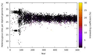
Figure 15: Individual heterozygosity index I_k measuring the proportion of loci that are at the heterozygous state in each individual of the population at the moment of their death. In this simulation, inbreeding was tolerated and the resulting inbreeding coefficient is shown using a color-code.

References

-
[1]
J. E. M. McGeoch, M. W. McGeoch,
Polymer
amide in the allende and murchison meteorites, Meteoritics & Planetary
Science 50 (12) (2015) 1971–1983.
arXiv:https://onlinelibrary.wiley.com/doi/pdf/10.1111/maps.12558,
doi:10.1111/maps.12558.
URL https://onlinelibrary.wiley.com/doi/abs/10.1111/maps.12558 - [2] M. H. Carr, M. J. S. Belton, C. R. Chapman, M. E. Davies, P. Geissler, R. Greenberg, A. S. McEwen, B. R. Tufts, R. Greeley, R. Sullivan, J. W. Head, R. T. Pappalardo, K. P. Klaasen, T. V. Johnson, J. Kaufman, D. Senske, J. Moore, G. Neukum, G. Schubert, J. A. Burns, P. Thomas, J. Veverka, Evidence for a subsurface ocean on Europa, Nature 391 (6665) (1998) 363–365. doi:10.1038/34857.
- [3] L. Iess, R. Jacobson, M. Ducci, D. Stevenson, J. Lunine, J. Armstrong, S. Asmar, P. Racioppa, N. Rappaport, P. Tortora, The tides of titan, Science (New York, N.Y.) 337 (2012) 457–9. doi:10.1126/science.1219631.
-
[4]
R. Orosei, S. E. Lauro, E. Pettinelli, A. Cicchetti, M. Coradini, B. Cosciotti,
F. Di Paolo, E. Flamini, E. Mattei, M. Pajola, F. Soldovieri, M. Cartacci,
F. Cassenti, A. Frigeri, S. Giuppi, R. Martufi, A. Masdea, G. Mitri,
C. Nenna, R. Noschese, M. Restano, R. Seu,
Radar evidence of
subglacial liquid water on mars, Science 361 (6401) (2018) 490–493.
arXiv:https://science.sciencemag.org/content/361/6401/490.full.pdf,
doi:10.1126/science.aar7268.
URL https://science.sciencemag.org/content/361/6401/490 - [5] A. M. Hein, M. Pak, D. Putz, C. Buhler, P. Reiss, World ships - architectures & feasibility revisited, Journal of the British Interplanetary Society 65 (2012) 119–133.
- [6] M. Fareed, M. Afzal, Genetics of consanguinity and inbreeding in health and disease, Annals of Human Biology 44 (2017) 99–107. doi:10.1080/03014460.2016.1265148.
- [7] D. Charlesworth, J. Willis, The genetics of inbreeding depression, Nature reviews. Genetics 10 (2009) 783–96. doi:10.1038/nrg2664.
- [8] I. Jamieson, F. Allendorf, How does the 50/500 rule apply to mvps?, Trends in ecology & evolution 27 (2012) 578–84. doi:10.1016/j.tree.2012.07.001.
- [9] R. Frankham, B. Brook, C. Bradshaw, L. Traill, D. Spielman, 50/500 rule and minimum viable populations: Response to jamieson and allendorf, Trends in ecology & evolution 28. doi:10.1016/j.tree.2013.01.002.
- [10] F. Marin, HERITAGE: A Monte Carlo code to evaluate the viability of interstellar travels using a multi-generational crew, Journal of the British Interplanetary Society 70 (2017) 184–195.
- [11] F. Marin, C. Beluffi, Computing the Minimal Crew for a multi-generational space journey towards Proxima b, Journal of the British Interplanetary Society 71 (2018) 45–52. arXiv:1806.03856.
- [12] F. Marin, C. Beluffi, R. Taylor, L. Grau, Numerical constraints on the size of generation ships from total energy expenditure on board, annual food production and space farming techniques, Journal of the British Interplanetary Society 71 (2018) 382–393. arXiv:1901.09542.
- [13] F. Marin, C. Beluffi, Water and air consumption aboard interstellar arks, arXiv e-prints (2020) arXiv:2003.09286arXiv:2003.09286.
-
[14]
S. Wright, Coefficients of
inbreeding and relationship, The American Naturalist 56 (645) (1922)
330–338.
URL http://www.jstor.org/stable/2456273 - [15] C. M. Smith, Estimation of a genetically viable population for multigenerational interstellar voyaging: Review and data for project Hyperion, Acta Astronautica 97 (2014) 16–29. doi:10.1016/j.actaastro.2013.12.013.
- [16] F. Ceballos, P. Joshi, D. Clark, M. Ramsay, J. Wilson, Runs of homozygosity: Windows into population history and trait architecture, Nature Reviews Genetics 19. doi:10.1038/nrg.2017.109.
-
[17]
J. T. Howard, J. E. Pryce, C. Baes, C. Maltecca,
Invited
review: Inbreeding in the genomics era: Inbreeding, inbreeding depression,
and management of genomic variability, Journal of Dairy Science 100 (8)
(2017) 6009 – 6024.
doi:https://doi.org/10.3168/jds.2017-12787.
URL http://www.sciencedirect.com/science/article/pii/S0022030217305817 -
[18]
H. L. Carson, The
genetic system, the deme, and the origin of species, Annual Review of
Genetics 21 (1) (1987) 405–423, pMID: 3327471.
arXiv:https://doi.org/10.1146/annurev.ge.21.120187.002201, doi:10.1146/annurev.ge.21.120187.002201.
URL https://doi.org/10.1146/annurev.ge.21.120187.002201 - [19] L. Palinkas, Psychosocial issues in long-term space flight: overview, Gravitational and space biology bulletin : publication of the American Society for Gravitational and Space Biology 14 (2001) 25–33.
- [20] D. Collins, Psychological issues relevant to astronaut selection for long-duration space flight: A review of the literature, Human performance in extreme environments : the journal of the Society for Human Performance in Extreme Environments 7 (2003) 43–67. doi:10.7771/2327-2937.1021.
- [21] N. Kanas, G. Sandal, B. Johannes, Psychology and culture during long-duration space missions, Psychology and and culture during long-duration space mission.
- [22] L. Landon, C. Rokholt, K. Slack, Y. Pecena, Selecting astronauts for long-duration exploration missions: Considerations for team performance and functioning, REACH - Reviews in Human Space Exploration 5. doi:10.1016/j.reach.2017.03.002.
- [23] C. Tafforin, F. Abati, Cultural ethology as a new approach of interplanetary crew’s behavior, Acta Astronautica 139. doi:10.1016/j.actaastro.2017.06.017.
- [24] L. Billings, How shall we live in space? culture, law and ethics in spacefaring society, Space Policy 22 (2006) 249–255. doi:10.1016/j.spacepol.2006.08.001.
- [25] J. Pass, Moon bases as initial” space society” trials: Utilizing astrosociology to make space settlements livable 8723. doi:10.1063/1.2437520.
- [26] C. Smith, E. Davies, Emigrating Beyond Earth, 2012. doi:10.1007/978-1-4614-1165-9.
-
[27]
C. Smith, Principles of
Space Anthropology: Establishing a Science of Human Space Settlement, Space
and Society, Springer International Publishing, 2019.
URL https://books.google.fr/books?id=AguwDwAAQBAJ -
[28]
G. R. Cutting,
Modifier
genetics: Cystic fibrosis, Annual Review of Genomics and Human Genetics
6 (1) (2005) 237–260, pMID: 15896111.
arXiv:https://doi.org/10.1146/annurev.genom.6.080604.162254, doi:10.1146/annurev.genom.6.080604.162254.
URL https://doi.org/10.1146/annurev.genom.6.080604.162254 -
[29]
U. Motro, G. Thomson,
On
heterozygosity and the effective size of populations subject to size
changes, Evolution 36 (5) (1982) 1059–1066.
arXiv:https://onlinelibrary.wiley.com/doi/pdf/10.1111/j.1558-5646.1982.tb05474.x,
doi:10.1111/j.1558-5646.1982.tb05474.x.
URL https://onlinelibrary.wiley.com/doi/abs/10.1111/j.1558-5646.1982.tb05474.x - [30] O. Mayo, A century of hardy–weinberg equilibrium, Twin research and human genetics : the official journal of the International Society for Twin Studies 11 (2008) 249–56. doi:10.1375/twin.11.3.249.
- [31] J. Zlotogora, G. Bach, The possibility of a selection process in the ashkenazi jewish population, American journal of human genetics 73 (2003) 438–40; author reply 440. doi:10.1086/377008.
- [32] T. Fournier, J. Schacherer, Genetic backgrounds and hidden trait complexity in natural populations, Current opinion in genetics & development 47 (2017) 48–53. doi:10.1016/j.gde.2017.08.009.
- [33] W. O’Neal, M. Knowles, Cystic fibrosis disease modifiers: Complex genetics defines the phenotypic diversity in a monogenic disease, Annual Review of Genomics and Human Genetics 19. doi:10.1146/annurev-genom-083117-021329.
- [34] R. Redon, S. Ishikawa, K. Fitch, L. Feuk, G. Perry, T. Andrews, H. Fiegler, M. Shapero, A. Carson, W. Chen, E. Cho, S. Dallaire, J. Freeman, J. Gonzalez, M. Gratacòs, J. Huang, D. Kalaitzopoulos, D. Komura, J. Macdonald, M. Hurles, Global variation in copy number in the human genome, Nature 444 (2006) 444–454. doi:10.1038/nature05329.
- [35] A. A, G. Abecasis, A. DM, D. RM, B. DR, C. A, C. AG, D. P, E. EE, F. P, G. SB, R. Gibbs, G. ED, H. ME, B. Knoppers, K. JO, L. ES, C. Lee, H. Lehrach, S. JA, A global reference for human genetic variation, Nature 526 (2015) 68.
-
[36]
G. H. Hardy, Mendelian
proportions in a mixed population, Science 28 (706) (1908) 49–50.
arXiv:https://science.sciencemag.org/content/28/706/49.full.pdf,
doi:10.1126/science.28.706.49.
URL https://science.sciencemag.org/content/28/706/49 - [37] W. Weinberg, Über den nachweis der vererbung beim menschen, Jahreshefte des Vereins Varterländische Naturkunde in Württemberg 64 (1908) 369–382.
- [38] R. A. Fisher, Xxi.—on the dominance ratio, Proceedings of the royal society of Edinburgh 42 (1923) 321–341.
- [39] S. Wright, Evolution in mendelian populations, Genetics 16 (2) (1931) 97.
-
[40]
B. Alberts, A. Johnson, J. Lewis, P. Walter, M. Raff, K. Roberts,
Molecular Biology of the
Cell 4th Edition: International Student Edition, Routledge, 2002.
URL https://books.google.fr/books?id=ozigkQEACAAJ - [41] F. Baudat, Y. Imai, B. de Massy, Meiotic recombination in mammals: Localization and regulation, Nature reviews. Genetics 14 (2013) 794–806. doi:10.1038/nrg3573.
- [42] E. Bolcun-Filas, M. Handel, Meiosis: The chromosomal foundation of reproduction, Biology of Reproduction 99. doi:10.1093/biolre/ioy021.
-
[43]
K. Högstrand, J. Böhme,
A determination of the
frequency of gene conversion in unmanipulated mouse sperm, Proceedings of
the National Academy of Sciences 91 (21) (1994) 9921–9925.
arXiv:https://www.pnas.org/content/91/21/9921.full.pdf, doi:10.1073/pnas.91.21.9921.
URL https://www.pnas.org/content/91/21/9921 -
[44]
F. Stahl,
Gene
conversion, in: S. Brenner, J. H. Miller (Eds.), Encyclopedia of Genetics,
Academic Press, New York, 2001, pp. 774 – 778.
doi:https://doi.org/10.1006/rwgn.2001.0503.
URL http://www.sciencedirect.com/science/article/pii/B0122270800005036 - [45] A. Harpak, X. Lan, Z. Gao, J. Pritchard, Frequent nonallelic gene conversion on the human lineage and its effect on the divergence of gene duplicates, Proceedings of the National Academy of Sciences 114 (2017) 201708151. doi:10.1073/pnas.1708151114.
- [46] R. Ganai, E. Johansson, Dna replication—a matter of fidelity, Molecular Cell 62 (2016) 745–755. doi:10.1016/j.molcel.2016.05.003.
- [47] W. Baarends, R. Van Der Laan, J. Grootegoed, Dna repair mechanisms and gametogenesis, Reproduction (Cambridge, England) 121 (2001) 31–9. doi:10.1530/rep.0.1210031.
- [48] N. Chatterjee, G. Walker, Mechanisms of dna damage, repair, and mutagenesis, Environmental and molecular mutagenesis 58. doi:10.1002/em.22087.
- [49] C. Campbell, E. Eichler, Properties and rates of germline mutations in humans, Trends in genetics : TIG 29. doi:10.1016/j.tig.2013.04.005.
- [50] H. Maki, Origins of spontaneous mutations: Specificity and directionality of base-substitution, frameshift, and sequence-substitution mutageneses, Annual review of genetics 36 (2002) 279–303. doi:10.1146/annurev.genet.36.042602.094806.
- [51] A. Bebenek, I. Ziuzia-Graczyk, Fidelity of dna replication—a matter of proofreading, Current Genetics 64. doi:10.1007/s00294-018-0820-1.
-
[52]
R. Okayasu,
Repair of
dna damage induced by accelerated heavy ions—a mini review, International
Journal of Cancer 130 (5) (2012) 991–1000.
arXiv:https://onlinelibrary.wiley.com/doi/pdf/10.1002/ijc.26445,
doi:10.1002/ijc.26445.
URL https://onlinelibrary.wiley.com/doi/abs/10.1002/ijc.26445 -
[53]
K. Sankaranarayanan, R. Taleei, S. Rahmanian, H. Nikjoo,
Ionizing
radiation and genetic risks. xvii. formation mechanisms underlying naturally
occurring dna deletions in the human genome and their potential relevance for
bridging the gap between induced dna double-strand breaks and deletions in
irradiated germ cells, Mutation Research/Reviews in Mutation Research
753 (2) (2013) 114 – 130.
doi:https://doi.org/10.1016/j.mrrev.2013.07.003.
URL http://www.sciencedirect.com/science/article/pii/S1383574213000501 - [54] J. Rak, L. Chomicz-Mańka, J. Wiczk, K. Westphal, M. Zdrowowicz, P. Wityk, M. Żyndul, S. Makurat, L. Golon, Mechanisms of damage to dna labeled with electrophilic nucleobases induced by ionizing or uv radiation, The journal of physical chemistry. B 119. doi:10.1021/acs.jpcb.5b03948.
- [55] C. S. Ku, E. Tan, D. Cooper, From the periphery to centre stage: De novo single nucleotide variants play a key role in human genetic disease, Journal of medical genetics 50. doi:10.1136/jmedgenet-2013-101519.
- [56] B. Weckselblatt, M. Rudd, Human structural variation: Mechanisms of chromosome rearrangements, Trends in genetics : TIG 31. doi:10.1016/j.tig.2015.05.010.
- [57] A. Newman, C. Steen, C. Liu, A. Gentles, A. Chaudhuri, F. Scherer, M. Khodadoust, M. Shahrokh Esfahani, B. Luca, D. Steiner, M. Diehn, A. Alizadeh, Determining cell type abundance and expression from bulk tissues with digital cytometry, Nature Biotechnology 37. doi:10.1038/s41587-019-0114-2.
- [58] R. Taylor, A. Pyle, H. Griffin, E. Blakely, J. Duff, L. He, T. Smertenko, C. Alston, V. Neeve, A. Best, J. Yarham, J. Kirschner, U. Schara, B. Talim, H. Topaloglu, I. Barić, E. Holinski-Feder, A. Abicht, B. Czermin, P. Chinnery, Use of whole-exome sequencing to determine the genetic basis of multiple mitochondrial respiratory chain complex deficiencies, JAMA : the journal of the American Medical Association 312 (2014) 68–77. doi:10.1001/jama.2014.7184.
- [59] S. Gunes, M. Alsadaanasan, A. Agarwal, Spermatogenesis, dna damage and dna repair mechanisms in male infertility, Reproductive BioMedicine Online 31. doi:10.1016/j.rbmo.2015.06.010.
- [60] J. Linsley, L. Scarsi, B. Rossi, Extremely Energetic Cosmic-Ray Event, Physical Review Letters 6 (9) (1961) 485–487. doi:10.1103/PhysRevLett.6.485.
- [61] J. Linsley, Evidence for a Primary Cosmic-Ray Particle with Energy 1e20 eV, Physical Review Letters 10 (4) (1963) 146–148. doi:10.1103/PhysRevLett.10.146.
- [62] A. H. Compton, H. A. Bethe, Composition of Cosmic Rays, Nature 134 (3393) (1934) 734–735. doi:10.1038/134734b0.
-
[63]
R. Mewaldt,
Galactic
cosmic ray composition and energy spectra, Advances in Space Research
14 (10) (1994) 737 – 747.
doi:https://doi.org/10.1016/0273-1177(94)90536-3.
URL http://www.sciencedirect.com/science/article/pii/0273117794905363 - [64] Pierre Auger Collaboration, Depth of Maximum of Air-Shower Profiles at the Pierre Auger Observatory: Composition Implications, arXiv e-prints (2014) arXiv:1409.5083arXiv:1409.5083.
- [65] Pierre Auger Collaboration, Observation of a large-scale anisotropy in the arrival directions of cosmic rays above 8e18 eV, Science 357 (6357) (2017) 1266–1270. arXiv:1709.07321, doi:10.1126/science.aan4338.
- [66] G. Nelson, Space radiation and human exposures, a primer, Radiation Research 185. doi:10.1667/RR14311.1.
-
[67]
C. Radiation, C. Sciences, D. Studies, N. Council,
Health Effects of
Exposure to Low Levels of Ionizing Radiation:: BEIR V, BEIR (Series),
National Academies Press, 1990.
URL https://books.google.fr/books?id=Kj0rAAAAYAAJ -
[68]
M. Frankenberg-Schwager, Induction,
repair and biological relevance of radiation-induced dna lesions in
eukaryotic cells, Radiation and Environmental Biophysics 29 (4) (1990)
273–292.
doi:10.1007/BF01210408.
URL https://doi.org/10.1007/BF01210408 - [69] M. Moreno-Villanueva, M. Wong, T. Lu, Y. Zhang, H. Wu, Interplay of space radiation and microgravity in dna damage and dna damage response, NPJ microgravity 3, article Number: 14. doi:10.1038/s41526-017-0019-7.
- [70] F. Tang, W.-K. Loke, Molecular mechanisms of low dose ionizing radiation-induced hormesis, adaptive responses, radioresistance, bystander effects, and genomic instability, International journal of radiation biology 91 (2014) 1–68. doi:10.3109/09553002.2014.937510.
- [71] M. Durante, F. Cucinotta, Heavy ion carcinogenesis and space exploration, Nature reviews. Cancer 8 (2008) 465–72. doi:10.1038/nrc2391.
- [72] M. Barcellos-Hoff, E. Blakely, S. Burma, A. Fornace, S. Gerson, L. Hlatky, D. Kirsch, U. Luderer, J. Shay, Y. Wang, M. Weil, Concepts and challenges in cancer risk prediction for the space radiation environment, Life sciences in space research 6 (2015) 92–103. doi:10.1016/j.lssr.2015.07.006.
- [73] D. Sridharan, A. Aroumougame, S. Bailey, S. Costes, P. Doetsch, W. Dynan, A. Kronenberg, K. Rithidech, J. Saha, A. Snijders, E. Werner, C. Wiese, F. Cucinotta, J. Pluth, Understanding cancer development processes after hze-particle exposure: Roles of ros, dna damage repair and inflammation, Radiation research 183. doi:10.1667/RR13804.1.
- [74] D. Sridharan, A. Aroumougame, S. Blattnig, S. Costes, P. Doetsch, W. Dynan, P. Hahnfeldt, L. Hlatky, Y. Kidane, A. Kronenberg, M. Naidu, L. Peterson, I. Plante, A. Ponomarev, J. Saha, A. Snijders, K. Srinivasan, J. Tang, E. Werner, J. Pluth, Evaluating biomarkers to model cancer risk post cosmic ray exposure, Life Sciences in Space Research 9. doi:10.1016/j.lssr.2016.05.004.
- [75] Z. Li, K. K. Jella, L. Jaafar, S. Li, S. Park, M. Story, H. Wang, Y. Wang, W. Dynan, Exposure to galactic cosmic radiation compromises dna repair and increases the potential for oncogenic chromosomal rearrangement in bronchial epithelial cells, Scientific Reports 8. doi:10.1038/s41598-018-29350-5.
- [76] F. Tang, W.-K. Loke, B. Khoo, Low-dose or low-dose-rate ionizing radiation-induced bioeffects in animal models, Journal of radiation research 58. doi:10.1093/jrr/rrw120.
- [77] F. Tang, K. Loganovsky, Low dose or low dose rate ionizing radiation-induced health effect in the human, Journal of Environmental Radioactivity 192. doi:10.1016/j.jenvrad.2018.05.018.
- [78] T. Squillaro, R. de rosa, G. Peluso, The effect of low-dose ionizing radiation on stem cell biology: A contribution to radiation risk: radiation risk and stem cells, STEM CELLS 36. doi:10.1002/stem.2836.
-
[79]
E. Cekanaviciute, S. Rosi, S. V. Costes,
Central
nervous system responses to simulated galactic cosmic rays., International
Journal of Molecular Sciences 19 (11) (2018) 3669.
URL http://scd-rproxy.u-strasbg.fr/login?url=http://search.ebscohost.com/login.aspx?direct=true&db=asx&AN=133157706&lang=fr&site=eds-live&scope=site - [80] R. Jandial, R. Hoshide, J. Waters, C. Limoli, Space–brain: The negative effects of space exposure on the central nervous system, Surgical Neurology International 9 (2018) 9. doi:10.4103/sni.sni_250_17.
- [81] P. Jacquet, Sensitivity of germ cells and embryos to ionizing radiation, Journal of biological regulators and homeostatic agents 18 (2004) 106–14.
- [82] R. Brent, Carcinogenic risks of prenatal ionizing radiation, Seminars in fetal & neonatal medicine 19. doi:10.1016/j.siny.2013.11.009.
- [83] N. Nakamura, A. Suyama, A. Noda, Y. Kodama, Radiation effects on human heredity, Annual review of genetics 47. doi:10.1146/annurev-genet-111212-133501.
- [84] B. Mishra, U. Luderer, Reproductive hazards of space travel in women and men, Nature Reviews Endocrinology 15. doi:10.1038/s41574-019-0267-6.
- [85] A. Adewoye, S. Lindsay, Y. Dubrova, M. Hurles, The genome-wide effects of ionizing radiation on mutation induction in the mammalian germline, Nature Communications 6 (2015) 6684. doi:10.1038/ncomms7684.
-
[86]
D. Delves, I. A. E. Agency,
IAEA Safety Glossary:
Terminology Used in Nuclear Safety and Radiation Protection, STI/PUB /
International Atomic Energy Agency, International Atomic Energy Agency, 2007.
URL https://books.google.fr/books?id=e65DOAAACAAJ -
[87]
G. Cinelli, V. Gruber, L. D. Felice, P. Bossew, M. A. Hernandez-Ceballos,
T. Tollefsen, S. Mundigl, M. D. Cort,
European annual
cosmic-ray dose: estimation of population exposure, Journal of Maps 13 (2)
(2017) 812–821.
arXiv:https://doi.org/10.1080/17445647.2017.1384934, doi:10.1080/17445647.2017.1384934.
URL https://doi.org/10.1080/17445647.2017.1384934 - [88] T. Ebisuzaki, S. Maruyama, United theory of biological evolution: Disaster-forced evolution through supernova, radioactive ash fall-outs, genome instability, and mass extinctions, Geoscience Frontiers 6. doi:10.1016/j.gsf.2014.04.009.
-
[89]
N. C. on Radiation Protection (NCRP),
Ionizing Radiation
Exposure of the Population of the United States, Vol. 93 of STI/PUB /
International Atomic Energy Agency, United States Nuclear Regulatory
Commission, 1987.
URL https://books.google.fr/books?id=e65DOAAACAAJ -
[90]
F. A. Cucinotta, M.-H. Y. Kim, V. Willingham, K. A. George,
Physical and Biological Organ
Dosimetry Analysis for International Space Station Astronauts, Radiation
Research 170 (1) (2008) 127 – 138.
doi:10.1667/RR1330.1.
URL https://doi.org/10.1667/RR1330.1 - [91] J. Chancellor, R. Blue, K. Cengel, S. Auñón-Chancellor, K. Rubins, H. Katzgraber, A. Kennedy, Limitations in predicting the space radiation health risk for exploration astronauts 8. doi:10.1038/s41526-018-0043-2.
-
[92]
Insee, Bilan
démographique 2018, Institut national de la statistique et des études
économiques.
URL https://www.insee.fr/fr/statistiques/1912926 -
[93]
J. Y. Ho, A. S. Hendi, Recent
trends in life expectancy across high income countries: retrospective
observational study, BMJ 362.
arXiv:https://www.bmj.com/content/362/bmj.k3622.full.pdf, doi:10.1136/bmj.k3622.
URL https://www.bmj.com/content/362/bmj.k3622 - [94] J. H. Moore, Kin-based crews for interstellar multi-generational space travel, in: K. Yoji, F. Bruhweiler, J. Moore, C. Sheffield (Eds.), Interstellar Travel and Multi-Generation Space Ships, Collectors Guide Publishing, Burlington, Ontario, Canada, 2003, pp. 80–88.
- [95] J. O. Deasy, Is monte carlo noise removal feasible?, in: W. Schlegel, T. Bortfeld (Eds.), The Use of Computers in Radiation Therapy, Springer Berlin Heidelberg, Berlin, Heidelberg, 2000, pp. 403–405.
-
[96]
B. J. Keats, S. L. Sherman,
Chapter
13 - population genetics, in: D. Rimoin, R. Pyeritz, B. Korf (Eds.), Emery
and Rimoin’s Principles and Practice of Medical Genetics, Academic Press,
Oxford, 2013, pp. 1 – 12.
doi:https://doi.org/10.1016/B978-0-12-383834-6.00015-X.
URL http://www.sciencedirect.com/science/article/pii/B978012383834600015X -
[97]
A. W. F. Edwards, G. h.
hardy (1908) and hardy–weinberg equilibrium, Genetics 179 (3)
(2008) 1143–1150.
arXiv:https://www.genetics.org/content/179/3/1143.full.pdf, doi:10.1534/genetics.104.92940.
URL https://www.genetics.org/content/179/3/1143 - [98] M. Nei, A. K. Roychoudhury, Genic variation within and between the three major races of man, caucasoids, negroids, and mongoloids., American journal of human genetics 26 4 (1974) 421–43.
- [99] M. Nei, Mathematical models of speciation and genetic distance, 1976, pp. 723–765.
- [100] N. Galtier, Delineating species in the speciation continuum: A proposal, Evolutionary Applications 12. doi:10.1111/eva.12748.
-
[101]
M. Kimura, T. Ohta, Stepwise mutation
model and distribution of allelic frequencies in a finite population,
Proceedings of the National Academy of Sciences of the United States of
America 75 (6) (1978) 2868–2872.
URL http://www.jstor.org/stable/68345 -
[102]
A. Fudala, R. Korona,
Low
frequency of mutations with strongly deleterious but nonlethal fitness
effects, Evolution 63 (8) (2009) 2164–2171.
arXiv:https://onlinelibrary.wiley.com/doi/pdf/10.1111/j.1558-5646.2009.00713.x,
doi:10.1111/j.1558-5646.2009.00713.x.
URL https://onlinelibrary.wiley.com/doi/abs/10.1111/j.1558-5646.2009.00713.x - [103] J. Masel, Q&a: Evolutionary capacitance, BMC biology 11 (2013) 103. doi:10.1186/1741-7007-11-103.
- [104] V. Ivanov, A. Tsyb, A. Gorsky, M. Maksyutov, E. M. Rastopchin, A. Konogorov, A. Korelo, A. Biryukov, V. t. Matyash, Leukaemia and thyroid cancer in emergency workers of the chernobyl accident, Radiation and environmental biophysics 36 (1) (1997) 9–16.
- [105] S. Davis, V. Stepanenko, N. Rivkind, K. J. Kopecky, P. Voillequé, V. Shakhtarin, E. Parshkov, S. Kulikov, E. Lushnikov, A. Abrosimov, et al., Risk of thyroid cancer in the bryansk oblast of the russian federation after the chernobyl power station accident, Radiation research 162 (3) (2004) 241–248.
-
[106]
L. B. Zablotska, 30 years
after the chernobyl nuclear accident: Time for reflection and re-evaluation
of current disaster preparedness plans, Journal of Urban Health 93 (3)
(2016) 407–413.
doi:10.1007/s11524-016-0053-x.
URL https://doi.org/10.1007/s11524-016-0053-x - [107] C. Rhodes, The fukushima daiichi nuclear accident, Science progress 97 (2014) 72–86. doi:10.3184/003685014X13904938571454.
-
[108]
W. Taira, C. Nohara, A. Hiyama, J. M. Otaki,
Fukushima’s Biological
Impacts: The Case of the Pale Grass Blue Butterfly, Journal of Heredity
105 (5) (2014) 710–722.
arXiv:http://oup.prod.sis.lan/jhered/article-pdf/105/5/710/10006420/esu013.pdf,
doi:10.1093/jhered/esu013.
URL https://doi.org/10.1093/jhered/esu013