A Modified Method of Successive Approximations for Stochastic Recursive Optimal Control Problems

Abstract. Based on the stochastic maximum principle for the partially coupled forward-backward stochastic control system (FBSCS for short), a modified method of successive approximations (MSA for short) is established for stochastic recursive optimal control problems. The second-order adjoint processes are introduced in the augmented Hamiltonian minimization step since the control domain is not necessarily convex. Thanks to the theory of bounded mean oscillation martingales (BMO martingales for short), we give a delicate proof of the error estimate and then prove the convergence of the modified MSA algorithm. In a special case, we obtain a logarithmic convergence rate. When the control domain is convex and compact, a sufficient condition which makes the control returned from the MSA algorithm be a near-optimal control is given for a class of linear FBSCSs.

Key words. BMO martingales; Forward-backward stochastic differential equations; Method of successive approximations; Stochastic maximum principle; Stochastic recursive optimal control

MSC subject classifications. 93E20, 60H10, 60H30, 49M05

1 Introduction

Finding numerical solutions to optimal control problems by scientific computing methods has attracted much attention in recent years. As one of those methods, the method of successive approximations (MSA for short) is an efficient tool to tackle optimal control problems. Compared with the algorithms based on the dynamic programming approach (for example, the Bellman-Howard policy iteration algorithm in [17]), the MSA is an iterative method equipped with alternating propagation and optimization steps based on the maximum principle. New application of the modified MSA to a deep learning problem has been investigated recently in [21], which leads to an alternative approach to training the deep neural networks from the deterministic optimal control viewpoint.

The MSA based on Pontryagin’s maximum principle [1] for seeking numerical solutions to deterministic control systems was first proposed by Krylov et al. [18]. This method includes successive integrations of the state and adjoint equations, and updates the control variables by minimizing the Hamiltonian. After that, many improved modifications of the MSA have been developed by researchers for a variety of deterministic control systems ([3, 19, 21, 22]).

A recent breakthrough in investigating the modified MSA for classical stochastic control systems can be found in [16], where the convergence result is based on the local stochastic maximum principle (SMP for short, see Theorem 4.12 in [2]). This provides a policy-updating algorithm to find the local optimal control candidates to the classical stochastic control systems, which improved their former result in [17] that is only capable of handling such kind of controlled dynamics with no control variables in the diffusion part. Nevertheless, in order to obtain the convergence of the modified MSA, the authors assumed "$D_{x}^{2}\sigma(\cdot)\equiv 0$" to eliminate the impact of the unboundedness of $q^{u}$ (see (2.8)) when they deduce the error estimates. Furthermore, since their modified MSA is based on the local SMP, it may fail to deal with the case when the control domain is non-convex. Thus, there are two natural questions that whether the above strong assumption can be weakened and how to modify the MSA to be applicable to the control problems with general control domains.

To go a further step, it has become increasingly clear that the modified MSA calls for an extension from the classical stochastic control system to a more general one with a non-convex control domain and weaker assumptions imposed on coefficients. Therefore, the main goal of this paper is to establish the modified MSA for the stochastic recursive optimal control problem which the state equation is described by a partially coupled forward-backward stochastic differential equation (FBSDE for short, see [11], [23], [31] and the references therein), and deduce the convergence of it. This kind of wider optimal control problem is closely related to the stochastic differential utility which plays an important role in the study of economic and financial fields such as the preference difference, the asset pricing, and the continuous-time general equilibrium in security markets (see [5, 14, 20] and the references therein).

More than that, we study the general case when the control domain may be non-convex. For this purpose, the construction of the modified MSA needs to base on the general SMP for the forward-backward stochastic control system (FBCSC for short). As for the general SMP, Peng [24] first established the general SMP for classical stochastic control systems. Then, numerous progress has been made for various stochastic control systems ([6, 25, 28, 29, 30]). Recently, Hu [9] introduced two adjoint equations to obtain the SMP for FBSCSs governed by partially coupled FBSDEs and solved the open problem proposed by Peng [26]. Inspired by Hu’s work, Hu et al. [10] lately proposed a new method to obtain the first and second-order variational equations which are essentially fully coupled FBSDEs, and derived the SMP for fully coupled FBSCSs.

Our main contributions are as follows. Firstly, we established a modified MSA for stochastic recursive optimal control problems subject to the partially coupled FBSCS (2.3) with a general control domain and proved it converges to a local minimum of the original control problem, which completely covers the results obtained in [16]. It is worth pointing out that the challenge to obtain the desired error estimate is the unboundedness of the solution $q^{u}$ to the adjoint equation (2.8). As mentioned earlier, this technical difficulty was avoided if we impose the restrictive assumption "$D_{x}^{2}\sigma(\cdot)\equiv 0$". Fortunately, we found that the stochastic integral $q^{u}\cdot W$ is a multi-dimensional BMO martingale, and substantially benefit from the harmonic analysis on the space of BMO martingales developed for tackling certain backward stochastic differential equations with unbounded coefficients by Delbaen and Tang [4]. Due to some useful inequalities, in particular the probabilistic version of Fefferman’s inequality, we obtained the error estimate which is critical to the convergence of our modified MSA. This also indicates that we can remove the above unnecessary assumption imposed on the diffusion coefficient by employing the BMO property of $q^{u}\cdot W$.

Secondly, in contrast to the classical stochastic control system, the emergence of $Z^{u}$ in the backward state equation of (2.3) makes the error estimate more difficult and complicated. By applying the Girsanov transformation, the process (3.10) disappears in the drift term under a new reference probability measure. It should be emphasized that the BMO property of any martingale under this new reference probability measure can be inherited from the corresponding one under the original probability measure. Then we get the error estimate (3.9) successfully. Furthermore, since the control domain need not be convex, the augmented Hamiltonian contains the second-order adjoint process $P^{u}$ (see (2.9)) whose boundedness is essential to obtain the error estimate (3.9). We proved that the boundedness of $P^{u}$ depends on the BMO property of $q^{u}\cdot W$.

Thirdly, as the number of the iterations $m$ increases, we obtain a $\frac{1}{m}$-order convergence rate of the stochastic control system only driven by a forward stochastic differential equation and the cost functional is quadratic both in the state and control processes. In addition, from the viewpoint of the near-optimality [32], we also prove the control returned from the MSA algorithm is near-optimal for a class of linear forward-backward stochastic recursive problems independent of $z$, when the control domain is convex and compact.

The rest of the paper is organized as follows. In section 2, preliminaries and the formulation of our problem are given. In section 3, we first show properties of the solutions to the adjoint equations, and then state our main results consisting of the error estimate and the convergence of our modified MSA algorithm. The results about the convergence rate and the sufficient condition of the near-optimality are also given as applications of the modified MSA algorithm. In section 4, we provide numerical demonstrations to illustrate the general results.

2 Preliminaries and Problem Formulation

Fix a terminal value $T>0$ and three positive integers $n$, $d$ and $k$. Let $(\Omega,\mathcal{F},\mathbb{P})$ be a complete probability space on which a standard $d$-dimensional Brownian motion $W=(W_{t}^{1},W_{t}^{2},...W_{t}^{d})_{t\in[0,T]}^{\intercal}$ is defined, and $\mathbb{F}:\mathbb{=}\left\{\mathcal{F}_{t}\right\}_{t\in[0,T]}$ be the $\mathbb{P}$-augmentation of the natural filtration generated by $W$.

Denote by $\mathbb{R}^{n}$ the $n$-dimensional real Euclidean space, $\mathbb{R}^{n\times m}$ the set of $n\times m$ real matrices ($n,m\geq 1$) and $\mathbb{S}^{n\times n}$ the set of all $n\times n$ symmetric matrices. The scalar product (resp. norm) of $A$, $B\in\mathbb{R}^{n\times m}$ is denoted by $\left(A,B\right)=\mathrm{tr}\{AB^{\intercal}\}$ (resp. $\left|A\right|=\sqrt{\mathrm{tr}\left\{AA^{\intercal}\right\}}$), where the superscript ^⊺ denotes the transpose of vectors or matrices. Denote by $I_{n}$ the $n\times n$ identity matrix.

For any given $p,q\geq 1$, we introduce the following Banach spaces.

$L_{\mathcal{F}_{T}}^{p}(\Omega;\mathbb{R}^{n})$: the space of $\mathcal{F}_{T}$-measurable $\mathbb{R}^{n}$-valued random variables $\xi$ such that $\mathbb{E}\left[\left|\xi\right|^{p}\right]<\infty$.

$L_{\mathcal{F}_{T}}^{\infty}(\Omega;\mathbb{R}^{n})$: the space of $\mathcal{F}_{T}$-measurable $\mathbb{R}^{n}$-valued random variables $\xi$ such that $\underset{\omega\in\Omega}{\mathrm{ess\leavevmode\nobreak\ sup}}\left|\xi(\omega)\right|<\infty$.

$L_{\mathcal{F}}^{\infty}([0,T];\mathbb{R}^{n})$: the space of $\mathbb{F}$-adapted $\mathbb{R}^{n}$-valued processes $\varphi$ defined on $[0,T]$ such that

$$\left\|\varphi\right\|_{\infty}:=\underset{(t,\omega)\in[0,T]\times\Omega}{\mathrm{ess\leavevmode\nobreak\ sup}}\left|\varphi_{t}\left(\omega\right)\right|<\infty.$$

$\mathcal{S}_{\mathcal{F}}^{p}([0,T];\mathbb{R}^{n})$: the space of $\mathbb{F}$-adapted $\mathbb{R}^{n}$-valued continuous processes $\varphi$ such that $\mathbb{E}\left[\sup\limits_{t\in[0,T]}\left|\varphi_{t}\right|^{p}\right]<\infty$.

$\mathcal{H}_{\mathcal{F}}^{p}([0,T];\mathbb{R}^{n})$: the space of $\mathbb{R}^{n}$-valued $\mathbb{F}$-martingales $M=\left(M^{1},\ldots,M^{n}\right)^{\intercal}$ with continuous pathes such that $M_{0}=0$ and $\left\|M\right\|_{\mathcal{H}^{p}}:=\left\|\sqrt{\mathrm{tr}\left\{\left\langle M\right\rangle_{T}\right\}}\right\|_{L^{p}}<\infty$, where

$$\left\langle M\right\rangle_{t}:=\left(\left\langle M^{i},M^{j}\right\rangle_{t}\right)_{1\leq i,j\leq n}\text{ \ for \ }t\in[0,T].$$

$\mathcal{M}^{p}(\mathbb{R}^{n\times d})$: the space of $\mathbb{R}^{n\times d}$-valued $\mathbb{F}$-progressively measurable processes $\varphi$ defined on $[0,T]$ such that

$$\left\|\varphi\right\|_{\mathcal{M}^{p}}:=\left(\mathbb{E}\left[\left(\int_{0}^{T}\left|\varphi_{t}\right|^{2}dt\right)^{\frac{p}{2}}\right]\right)^{\frac{1}{p}}<\infty.$$

$\mathrm{BMO}$: the space of processes $M\in\mathcal{H}_{\mathcal{F}}^{2}([0,T];\mathbb{R})$ such that

$$\left\|M\right\|_{\mathrm{BMO}}:=\sup_{\tau}\left\|\left(\mathbb{E}\left[\left\langle M\right\rangle_{T}-\left\langle M\right\rangle_{\tau}\mid\mathcal{F}_{\tau}\right]\right)^{\frac{1}{2}}\right\|_{\infty}<\infty,$$ (2.1)

where the supremum is taken over all stopping times $\tau\in\mathcal{[}0,T\mathcal{]}$. Furthermore, one can replace $\tau$ with all deterministic times $t\in[0,T]$ in definition (2.1).

$\mathcal{K}(\mathbb{R}^{n\times d})$: the space of $\mathbb{R}^{n\times d}$-valued processes $\varphi\in\mathcal{M}^{2}(\mathbb{R}^{n\times d})$ such that

$$\left\|\varphi\right\|_{\mathcal{K}}:=\sup_{\tau}\left\|\left(\mathbb{E}\left[\int_{\tau}^{T}\left|\varphi_{s}\right|^{2}ds\mid\mathcal{F}_{\tau}\right]\right)^{\frac{1}{2}}\right\|_{\infty}<\infty,$$ (2.2)

where the supremum is taken over all stopping times $\tau\in\mathcal{[}0,T\mathcal{]}$. Furthermore, one can replace $\tau$ with all deterministic times $t\in[0,T]$ in definition (2.2).

We write $\mathrm{BMO}(\mathbb{Q})$ and $\mathcal{K}(\mathbb{R}^{n\times d};\mathbb{Q})$ for any probability $\mathbb{Q}$ defined on $\left(\Omega,\mathcal{F}\right)$ whenever it is necessary to indicate the underlying probability. For simplicity, if the underlying probability is $\mathbb{P}$, we still use the notations $\mathrm{BMO}$ and $\mathcal{K}(\mathbb{R}^{n\times d})$.

2.1 Some Notations and Results of BMO Martingales

Here we list some notations and results of BMO martingales, which will be used in this paper. We refer the readers to [4], [8], [15] the references therein for more details.

Denote by $\mathcal{E}\left(M\right)$ the Doléans-Dade exponential of a continuous local martingale $M$, that is, $\mathcal{E}\left(M_{t}\right)=\exp\left\{M_{t}-\frac{1}{2}\left\langle M\right\rangle_{t}\right\}$ for any $t\in[0,T].$ If $M\in\mathrm{BMO}$, then $\mathcal{E}(M)$ is a uniformly integrable martingale (see Theorem 2.3 in [15]).

Let $H$ be an $\mathbb{R}^{d}$-valued $\mathbb{F}$-adapted process. Denote by $H\cdot W$ the stochastic integral of $H$ with respect to the $d$-dimensional Brownian motion $W$, that is, $\left(H\cdot W\right)_{t}:=\sum_{i=1}^{d}\int_{0}^{t}H_{s}^{i}dW_{s}^{i}$ for $t\in[0,T]$.

The following theorem plays an significant role in characterizing the duality between $\mathcal{H}_{\mathcal{F}}^{1}([0,T];\mathbb{R})$ and $\mathrm{BMO}$.

Theorem 2.1 ([8], Theorem 10.18).

Let $N\in\mathcal{H}_{\mathcal{F}}^{1}([0,T];\mathbb{R})$, $M\in\mathrm{BMO}$, and $\varphi$ be an $\mathbb{F}$-progressive measurable process such that $\mathbb{E}\left[\left(\int_{0}^{T}\left|\varphi_{t}\right|^{2}d\langle N\rangle_{t}\right)^{\frac{1}{2}}\right]<\infty$. Then, for any stopping time $\tau$ in $[0,T]$,

$$\mathbb{E}\left[\int_{\tau}^{T}\left|\varphi_{s}\right|\left|d\left\langle M,N\right\rangle_{s}\right|\mid\mathcal{F}_{\tau}\right]\leq\sqrt{2}\mathbb{E}\left[\left(\int_{\tau}^{T}\left|\varphi_{s}\right|^{2}d\left\langle N\right\rangle_{s}\right)^{\frac{1}{2}}\mid\mathcal{F}_{\tau}\right]\left\|M\right\|_{\mathrm{BMO}}.$$

Particularly, when $\tau=0$ and $\varphi=1$, we have

$$\mathbb{E}\left[\int_{0}^{T}\left|d\left\langle M,N\right\rangle_{s}\right|\right]\leq\sqrt{2}\left\|M\right\|_{\mathrm{BMO}}\left\|N\right\|_{\mathcal{H}^{1}},$$

which is well known as Fefferman’s inequality.

For any $M\in\mathrm{BMO}$, the energy-type inequality for $\left\langle M\right\rangle$ is a significant result commonly used in the BMO martingale theory (see [15]). In essence, for any $\varphi\in\mathcal{K}(\mathbb{R}^{n\times d})$, $\mathbb{F}$-stopping time $\tau$ on $[0,T]$ and $A\in\mathcal{F}_{\tau}$, we can apply Garsia’s Lemma ([8], Lemma 10.35) to the continuous increasing process $\left(1_{A}\int_{\tau}^{t}\left|\varphi_{s}\right|^{2}ds\right)_{t\in[\tau,T]}$ to obtain the following energy-type inequality.

Proposition 2.2 (Energy inequality).

Let $\varphi\in\mathcal{K}(\mathbb{R}^{n\times d})$. Then, for any integer $m$ and $\mathbb{F}$-stopping time $\tau$ on $[0,T]$, we have

$$\mathbb{E}\left[\left(\int_{\tau}^{T}\left|\varphi_{s}\right|^{2}ds\right)^{m}\mid\mathcal{F}_{\tau}\right]\leq m!\left\|\varphi\right\|_{\mathcal{K}}^{2m}.$$

Recall that the space BMO depends on the underlying probability measure. The following lemma shows the equivalence of different BMO-norms under the Girsanov transformation.

Lemma 2.3 ([12], Lemma A.4).

Let $K>0$ be a given constant and $M$ be in BMO. Then, there are constants $c_{1}>0$ and $c_{2}>0$ depending only on $K$ such that for any $N\in\mathrm{BMO}$ and $\left\|N\right\|_{\mathrm{BMO}}\leq K$, we have

$$c_{1}\left\|M\right\|_{\mathrm{BMO}}\leq\left\|\tilde{M}\right\|_{\mathrm{BMO}(\mathbb{\tilde{P}})}\leq c_{2}\left\|M\right\|_{\mathrm{BMO}},$$

where $\tilde{M}:=M-\left\langle M,N\right\rangle$ and $d\mathbb{\tilde{P}}:=\mathcal{E}\left(N_{T}\right)d\mathbb{P}$.

The following proposition is a more profound result by applying Fefferman’s inequality.

Proposition 2.4 ([4], Lemma 1.4).

Let $p\geq 1$. Assume that $X\in\mathcal{S}_{\mathcal{F}}^{p}([0,T];\mathbb{R})$ and $M\in\mathrm{BMO}$. Then, $X\cdot M\in\mathcal{H}_{\mathcal{F}}^{p}([0,T];\mathbb{R})$. Moreover, we have the following estimate

$$\left\|X\cdot M\right\|_{\mathcal{H}^{p}}\leq\sqrt{2}\left\|X\right\|_{\mathcal{S}^{p}}\left\|M\right\|_{\mathrm{BMO}}$$

for $p>1$ and

$$\left\|X\cdot M\right\|_{\mathcal{H}^{1}}\leq\left\|X\right\|_{\mathcal{S}^{1}}\left\|M\right\|_{\mathrm{BMO}}.$$

2.2 Problem Formulation

Consider the following decoupled FBSCS:

$$\left\{\begin{array}[c]{rl}dX_{t}^{u}=&b(t,X_{t}^{u},u_{t})dt+\sigma(t,X_{t}^{u},u_{t})dW_{t},\\ dY_{t}^{u}=&-f(t,X_{t}^{u},Y_{t}^{u},Z_{t}^{u},u_{t})dt+\left(Z_{t}^{u}\right)^{\intercal}dW_{t},\\ X_{0}^{u}=&x_{0},\ Y_{T}^{u}=\Phi(X_{T}^{u}),\end{array}\right.$$ (2.3)

with the cost functional

$$J(u(\cdot)):=Y_{0}^{u}$$ (2.4)

for a given $x_{0}\in\mathbb{R}^{n}$ and measurable functions $b:[0,T]\times\mathbb{R}^{n}\times U\longmapsto\mathbb{R}^{n}$, $\sigma:[0,T]\times\mathbb{R}^{n}\times U\longmapsto\mathbb{R}^{n\times d}$, $f:[0,T]\times\mathbb{R}^{n}\times\mathbb{R}\times\mathbb{R}^{d}\times U\longmapsto\mathbb{R}$ and $\Phi:\mathbb{R}^{n}\longmapsto\mathbb{R}$, where the control domain $U$ is a nonempty subset of $\mathbb{R}^{k}$, and the $\mathbb{F}$-adapted process $u(\cdot)$ is called an admissible control which takes values in $U$ satisfying

$$\sup_{t\in[0,T]}\mathbb{E}\left[\left|u_{t}\right|^{8}\right]<\infty.$$ (2.5)

Denote by $\mathcal{U}[0,T]$ the set of all admissible controls, and assume $\inf_{u(\cdot)\in\mathcal{U}[0,T]}J\left(u(\cdot)\right)>-\infty$. We want to find an optimal control $\bar{u}(\cdot)\in\mathcal{U}[0,T]$ reaching the minimum of (2.4) or, if the minimum cannot be reached, an $\epsilon$-optimal control $u^{\epsilon}(\cdot)$ such that $J(u^{\epsilon}(\cdot))\leq\inf_{u(\cdot)\in\mathcal{U}[0,T]}J\left(u(\cdot)\right)+\epsilon$ for some given $\epsilon>0$.

For deterministic control systems, it has been shown that the basic MSA may diverge when a bad initial value of control is chosen (see [3]) or the feasibility errors blow up (see [21]). It can be observed that Kerimkulov et al. [16] proposed directly a modified MSA for classical stochastic control systems to ensure the convergence. To go a further step, we are aimed at establishing a modified MSA for stochastic recursive control optimal control problems and obtaining the related convergence result.

Before giving the modified MSA algorithm for (2.3), we first introduce the SMP for it. Set

$$\begin{array}[c]{l}b(\cdot)=\left(b^{1}(\cdot),b^{2}(\cdot),\ldots,b^{n}(\cdot)\right)^{\intercal}\in\mathbb{R}^{n},\\ \sigma(\cdot)=\left(\sigma^{1}(\cdot),\sigma^{2}(\cdot),\ldots,\sigma^{d}(\cdot)\right)\in\mathbb{R}^{n\times d},\\ \sigma^{i}(\cdot)=\left(\sigma^{1i}(\cdot),\sigma^{2i}(\cdot),\ldots,\sigma^{ni}(\cdot)\right)^{\intercal}\in\mathbb{R}^{n},\text{ }i=1,2,\ldots,d\end{array}$$

and impose the following assumptions on the coefficients of (2.3):

Assumption 2.5.

Let $L_{i},i=1,2,3$ be given positive constants.

(i) $b$ and $\sigma$ are twice continuously differentiable with respect to $x$. $b$, $\sigma$, $b_{x}$, $\sigma_{x}$, $b_{xx}$, $\sigma_{xx}$ are continuous in $\left(x,u\right)$. $b_{x}$, $\sigma_{x}$, $b_{xx}$, $\sigma_{xx}$ are bounded. $b$ and $\sigma$ are bounded by $L_{1}\left(1+\left|x\right|+\left|u\right|\right)$.

(ii) $\Phi$ is twice continuously differentiable with respect to $x$. $\Phi_{x}$, $\Phi_{xx}$ are bounded, and $\Phi$ is bounded by $L_{2}\left(1+\left|x\right|\right)$.

(iii) $f$ is twice continuously differentiable with respect to $(x,y,z)$. $f$ together with its gradient $Df$, Hessian matrix $D^{2}f$ with respect to $x$, $y$, $z$ are continuous in $(x,y,z,u)$. $Df$, $D^{2}f$ are bounded, and $f$ is bounded by $L_{3}\left(1+\left|x\right|+\left|y\right|+\left|z\right|+\left|u\right|\right)$.

Let us fix a $u(\cdot)\in\mathcal{U}[0,T]$ arbitrarily. Under Assumption 2.5, thanks to [27] (Chapter V, Theorem 6) and Theorem 5.1 in [14], (2.3) admits a unique solution $(X^{u},Y^{u},Z^{u})\in\mathcal{S}_{\mathcal{F}}^{2}([0,T];\mathbb{R}^{n})\times\mathcal{S}_{\mathcal{F}}^{2}([0,T];\mathbb{R})\times$ $\mathcal{M}^{2}(\mathbb{R}^{d})$. We call $(X^{u},Y^{u},Z^{u})$ the state trajectory corresponding to $u(\cdot)$. Particularly, let $\bar{u}(\cdot)$ be an optimal control, $\left(\bar{X},\bar{Y},\bar{Z}\right)$ be the corresponding state trajectory of (2.3) and $\left(\bar{p},\bar{q}\right)$, $\left(\bar{P},\bar{Q}\right)$ be the corresponding unique solution to the first-order adjoint equation (2.8), the second-order adjoint equation (2.9) below respectively. The (stochastic) Hamiltonian $H:[0,T]\times\Omega\times\mathbb{R}^{n}\times\mathbb{R}\times\mathbb{R}^{d}\times\mathbb{R}^{n}\times\mathbb{R}^{n\times d}\times\mathbb{R}^{n\times n}\times U\longmapsto\mathbb{R}$ is defined as follows:

$$H(t,x,y,z,p,q,P,u)$$

$$=\dfrac{1}{2}\sum\limits_{i=1}^{d}\left(\sigma^{i}(t,x,u)-\sigma^{i}(t,\bar{X}_{t},\bar{u}_{t})\right)^{\intercal}P\left(\sigma^{i}(t,x,u)-\sigma^{i}(t,\bar{X}_{t},\bar{u}_{t})\right)$$

$$+p^{\intercal}b(t,x,u)+\sum\limits_{i=1}^{d}\left(q^{i}\right)^{\intercal}\sigma^{i}(t,x,u)+f(t,x,y,z+\Delta(t,x,u),u),$$

where $q^{i}$ is the $i$th column of $q$ for $i=1,2,\ldots,d$, and

$$\Delta(t,x,u)=\left(\left(\sigma^{1}(t,x,u)-\sigma^{1}(t,\bar{X}_{t},\bar{u}_{t})\right)^{\intercal}p,\ldots,\left(\sigma^{d}(t,x,u)-\sigma^{d}(t,\bar{X}_{t},\bar{u}_{t})\right)^{\intercal}p\right)^{\intercal}.$$

Then the following stochastic maximum principle ([9], Theorem 3; [10], Theorem 3.17) holds.

Theorem 2.6.

Let Assumption 2.5 hold. Then, for all $u\in U$,

$$H(t,\bar{X}_{t},\bar{Y}_{t},\bar{Z}_{t},\bar{p}_{t},\bar{q}_{t},\bar{P}_{t},u)\geq H(t,\bar{X}_{t},\bar{Y}_{t},\bar{Z}_{t},\bar{p}_{t},\bar{q}_{t},\bar{P}_{t},\bar{u}_{t}),\ dt\otimes d\mathbb{P}\text{-}a.e..$$ (2.6)

Secondly, it follows from the pioneering works mentioned before that a key step to control the divergent behavior rigorously of the modified MSA is to obtain the error estimate by estimating the difference between two cost functionals $J(u(\cdot))$ and $J(v(\cdot))$ corresponding to different admissible controls $u(\cdot)$ and $v(\cdot)$. In order to do this, we need to introduce the following notations and the augmented Hamiltonian.

Define the function $G:[0,T]\times\mathbb{R}^{n}\times\mathbb{R}\times\mathbb{R}^{d}\times\mathbb{R}^{n}\times\mathbb{R}^{n\times d}\times U\times U\longmapsto\mathbb{R}$ by

$$G(t,x,y,z,p,q,v,u)=p^{\intercal}b(t,x,v)+\sum\limits_{i=1}^{d}\left(q^{i}\right)^{\intercal}\sigma^{i}(t,x,v)+f(t,x,y,z+\tilde{\Delta}(t,x,p,v,u),v),$$

where $q=\left(q^{1},\ldots,q^{d}\right)$ and

$$\tilde{\Delta}(t,x,p,v,u):=\left(\left(\sigma^{1}(t,x,v)-\sigma^{1}(t,x,u)\right)^{\intercal}p,\ldots,\left(\sigma^{d}(t,x,v)-\sigma^{d}(t,x,u)\right)^{\intercal}p\right)^{\intercal}.$$

Let $u(\cdot),v(\cdot)\in\mathcal{U}[0,T]$. For $\psi=b$, $\sigma$, and $w=x$, $y$, $z$, we simply set

$$\begin{array}[c]{ll}\Theta_{t}^{u}=\left(X_{t}^{u},Y_{t}^{u},Z_{t}^{u}\right),&\Theta_{t}^{u,v}=\left(X_{t}^{u},Y_{t}^{u},Z_{t}^{u}+\tilde{\Delta}(t,X_{t}^{u},p_{t}^{u},v_{t},u_{t})\right),\\ \psi^{u}(t)=\psi(t,X_{t}^{u},u_{t}),&\psi_{x}^{u}(t)=\psi_{x}(t,X_{t}^{u},u_{t}),\\ \psi_{xx}^{u}(t)=\psi_{xx}(t,X_{t}^{u},u_{t}),&\\ f^{u}(t)=f(t,\Theta_{t}^{u},u_{t}),&f^{u,v}(t)=f(t,\Theta_{t}^{u,v},v_{t}),\\ f_{w}^{u}(t)=f_{w}(t,\Theta_{t}^{u},u_{t}),&f_{w}^{u,v}(t)=f_{w}(t,\Theta_{t}^{u,v},v_{t}),\\ f_{ww}^{u}(t)=f_{ww}(t,\Theta_{t}^{u},u_{t}),&f_{ww}^{u,v}(t)=f_{ww}(t,\Theta_{t}^{u,v},v_{t})\end{array}$$ (2.7)

and $D^{2}f^{u}(t)=D^{2}f(t,\Theta_{t}^{u},u_{t})$ for all $t\in[0,T]$. In particular, for $i=1,\ldots,d$, we denote $\sigma_{x}^{u,i}(t)=\sigma_{x}^{i}(t,X_{t}^{u},u_{t})$ and $\sigma_{xx}^{u,i}(t)=\sigma_{xx}^{i}(t,X_{t}^{u},u_{t})$.

In our context, for $t\in[0,T]$, the first-order (resp. second-order) adjoint equation in [9] can be rewritten as (2.8) (resp. (2.9)) below.

$$\begin{array}[c]{rl}p_{t}^{u}=&\Phi_{x}(X_{T}^{u})+\int_{t}^{T}\left\{G_{x}(s,\Theta_{s}^{u},p_{s}^{u},q_{s}^{u},u_{s},u_{s})+G_{y}(s,\Theta_{s}^{u},p_{s}^{u},q_{s}^{u},u_{s},u_{s})p_{s}^{u}\right.\\ &+\left.\Upsilon(s,X_{s}^{u},p_{s}^{u},q_{s}^{u},u_{s})G_{z}(s,\Theta_{s}^{u},p_{s}^{u},q_{s}^{u},u_{s},u_{s})\right\}ds-\sum\limits_{i=1}^{d}\int_{t}^{T}\left(q_{s}^{u}\right)^{i}dW_{s}^{i},\end{array}$$ (2.8)

$$\begin{array}[c]{cl}P_{t}^{u}=&\Phi_{xx}(X_{T}^{u})+\int_{t}^{T}\left\{f_{y}^{u}(s)P_{s}^{u}+\left(b_{x}^{u}(s)\right)^{\intercal}P_{s}^{u}+\left(P_{s}^{u}\right)^{\intercal}b_{x}^{u}(s)\right.\\ &+\sum\limits_{i=1}^{d}f_{z_{i}}^{u}(s)\left[\left(\sigma_{x}^{u,i}(s)\right)^{\intercal}P_{s}^{u}+\left(P_{s}^{u}\right)^{\intercal}\sigma_{x}^{u,i}(s)\right]\\ &+\sum\limits_{i=1}^{d}\left(\sigma_{x}^{u,i}(s)\right)^{\intercal}P_{s}^{u}\sigma_{x}^{u,i}(s)+\sum\limits_{i=1}^{d}f_{z_{i}}^{u}(s)\left(Q_{s}^{u}\right)^{i}\\ &+\left.\sum\limits_{i=1}^{d}\left[\left(\sigma_{x}^{u,i}(s)\right)^{\intercal}\left(Q_{s}^{u}\right)^{i}+\left(\left(Q_{s}^{u}\right)^{i}\right)^{\intercal}\sigma_{x}^{u,i}(s)\right]+\Psi_{s}^{u}\right\}ds\\ &-\sum\limits_{i=1}^{d}\int_{t}^{T}\left(Q_{s}^{u}\right)^{i}dW_{s}^{i},\end{array}$$ (2.9)

where

$$\Upsilon(t,X_{t}^{u},p_{t}^{u},q_{t}^{u},u_{t})=\left(\left(\sigma_{x}^{1}(t,X_{t}^{u},u_{t})\right)^{\intercal}p_{t}^{u}+\left(q_{t}^{u}\right)^{1},\ldots,\left(\sigma_{x}^{d}(t,X_{t}^{u},u_{t})\right)^{\intercal}p_{t}^{u}+\left(q_{t}^{u}\right)^{d}\right),$$

$$\begin{array}[c]{rl}\Psi_{t}^{u}=&\sum\limits_{j=1}^{n}\left(b_{xx}^{u}(t)\right)^{j}\left(p_{t}^{u}\right)^{j}+\sum\limits_{i=1}^{d}\sum\limits_{j=1}^{n}\left(\sigma_{xx}^{u,i}(t)\right)^{j}\left(f_{z_{i}}^{u}(t)\left(p_{t}^{u}\right)^{j}+\left(q_{t}^{u}\right)^{ji}\right)\\ &+\left(I_{n},p_{t}^{u},\Upsilon(t,X_{t}^{u},p_{t}^{u},q_{t}^{u},u_{t})\right)D^{2}f^{u}(t)\left(I_{n},p_{t}^{u},\Upsilon(t,X_{t}^{u},p_{t}^{u},q_{t}^{u},u_{t})\right)^{\intercal}.\end{array}$$ (2.10)

Here, for $i=1,\ldots,d$ and $j=1,\ldots,n$, $\left(p^{u}\right)^{j}$, $\left(q^{u}\right)^{ji}$ are the $j$th components of $p^{u}$, $\left(q^{u}\right)^{i}$ respectively; $\left(b_{xx}^{u}(t)\right)^{j}$, $\left(\sigma_{xx}^{u,i}(t)\right)^{j}$ are the Hessian matrices of the $j$th components of $b^{u}(t)$, $\sigma^{u,i}(t)$ respectively.

Define the (deterministic) Hamiltonian $\mathcal{H}:[0,T]\times\mathbb{R}^{n}\times\mathbb{R}\times\mathbb{R}^{d}\times\mathbb{R}^{n}\times\mathbb{R}^{n\times d}\times\mathbb{R}^{n\times n}\times U\times U\longmapsto\mathbb{R}$ by

$$\begin{array}[c]{ll}&\mathcal{H}(t,x,y,z,p,q,P,v,u)\\ =&G(t,x,y,z,p,q,v,u)\\ &+\dfrac{1}{2}\sum\limits_{i=1}^{d}\left(\sigma^{i}(t,x,v)-\sigma^{i}(t,x,u)\right)^{\intercal}P\left(\sigma^{i}(t,x,v)-\sigma^{i}(t,x,u)\right).\end{array}$$ (2.11)

Then, for all $u\in U$, the SMP in Theorem 2.6 can be rewritten as follows:

$$\mathcal{H}(t,\bar{X}_{t},\bar{Y}_{t},\bar{Z}_{t},\bar{p}_{t},\bar{q}_{t},\bar{P}_{t},u,\bar{u}_{t})\geq\mathcal{H}(t,\bar{X}_{t},\bar{Y}_{t},\bar{Z}_{t},\bar{p}_{t},\bar{q}_{t},\bar{P}_{t},\bar{u}_{t},\bar{u}_{t}),\text{ }dt\otimes d\mathbb{P}\text{-}a.e..$$

Now we introduce the augmented Hamiltonian $\mathcal{\tilde{H}}:[0,T]\times\mathbb{R}^{n}\times\mathbb{R}\times\mathbb{R}^{d}\times\mathbb{R}^{n}\times\mathbb{R}^{n\times d}\times\mathbb{R}^{n\times n}\times U\times U\longmapsto\mathbb{R}$ for some $\rho\geq 0$ by

$$\begin{array}[c]{cl}&\mathcal{\tilde{H}(}t,x,y,z,p,q,P,v,u\mathcal{)}\\ =&\mathcal{H}(t,x,y,z,p,q,P,v,u)+\dfrac{\rho}{2}\left\{\sum\limits_{\psi\in\{b,\sigma,f\}}\left|\psi(t,x,y,z,v)-\psi(t,x,y,z,u)\right|^{2}\right.\\ &+\left.\sum\limits_{w\in\{x,y,z\}}\left|G_{w}(t,x,y,z,p,q,v,u)-G_{w}(t,x,y,z,p,q,u,u)\right|^{2}\right\}.\end{array}$$ (2.12)

Note that when $\rho=0$ we get exactly the Hamiltonian (2.11). Moreover, the SMP also holds for $\mathcal{\tilde{H}}$, which is a basis of constructing the iterations in the MSA algorithm.

Lemma 2.7 (Extended SMP).

Let $\bar{u}(\cdot)$ be an optimal control, $\left(\bar{X},\bar{Y},\bar{Z}\right)$ be the corresponding state trajectory of (2.3) and $\left(\bar{p},\bar{q}\right)$, $\left(\bar{P},\bar{Q}\right)$ be the corresponding unique solutions to (2.8), (2.9) respectively. Then we have, $dt\otimes d\mathbb{P}\text{-}a.e.$,

$$\mathcal{\tilde{H}}(t,\bar{X}_{t},\bar{Y}_{t},\bar{Z}_{t},\bar{p}_{t},\bar{q}_{t},\bar{P}_{t},\bar{u}_{t},\bar{u}_{t})=\min_{u\in U}\mathcal{\tilde{H}}(t,\bar{X}_{t},\bar{Y}_{t},\bar{Z}_{t},\bar{p}_{t},\bar{q}_{t},\bar{P}_{t},u,\bar{u}_{t}).$$ (2.13)

The proof of the extended SMP is a direct application of Theorem 2.6 and (2.12) so we omit it. It should be emphasized that not all the multiples such as $\left(\bar{X},\bar{Y},\bar{Z},\bar{p},\bar{q},\bar{P},\bar{u}(\cdot)\right)$ satisfying (2.13) are globally optimal for (2.3)-(2.4) since (2.6) is only the necessary condition of the optimality and (2.13) is weaker than (2.6). Nonetheless, we will lately obtain an “approximation” form of (2.13) in Theorem 3.4, which is helpful for us to derive the sufficient condition of the near-optimality for a class of linear forward-backward stochastic recursive control problems and it will be proved rigorously in Theorem 3.11.

As the end of this section, we introduce the modified MSA in the following algorithm.

  Algorithm 1 The Modified Method of Successive Approximations for Stochastic Recursive Optimal Control Problems

 

1:Variable Initialisation: Put $m=1$, and take any $u^{0}(\cdot)\in\mathcal{U}[0,T]$ to be an initial approximation.

2:Solve the FBSDE (2.3) corresponding to $u^{0}(\cdot)$ and then obtain the state trajectory $\left(X^{1},Y^{1},Z^{1}\right)$.

3:Calculate $J(u^{0}(\cdot))$.

4:Solve the BSDE (2.8) and (2.9) with the control $u^{0}(\cdot)$ and state trajectory $\left(X^{1},Y^{1},Z^{1}\right)$, and then obtain the first and second-order adjoint processes $\left(p^{1},q^{1}\right)$ and $\left(P^{1},Q^{1}\right)$.

5:Set

$$u_{t}^{1}\in\arg\min_{u\in U}\mathcal{\tilde{H}}(t,X_{t}^{1},Y_{t}^{1},Z_{t}^{1},p_{t}^{1},q_{t}^{1},P_{t}^{1},u,u_{t}^{0}),\quad t\in[0,T].$$

6:Repeat steps 2-3 by replacing $u^{0}(\cdot)$ with $u^{1}(\cdot)$, and then obtain $\left(X^{2},Y^{2},Z^{2}\right)$, $J(u^{1}(\cdot))$.

7:while $J(u^{m-1}(\cdot))-J(u^{m}(\cdot))$ is larger than some given permissible error $\epsilon>0$ do

8:     Increase the value of $m$ by $1$.

9:     Repeat the step 4 by replacing $u^{0}(\cdot)$, $\left(X^{1},Y^{1},Z^{1}\right)$ with $u^{m-1}(\cdot)$, $\left(X^{m},Y^{m},Z^{m}\right)$ respectively, and then obtain $\left(p^{m},q^{m}\right)$ and $\left(P^{m},Q^{m}\right)$.

10:     Update the control

$$u_{t}^{m}\in\arg\min_{u\in U}\mathcal{\tilde{H}}(t,X_{t}^{m},Y_{t}^{m},Z_{t}^{m},p_{t}^{m},q_{t}^{m},P_{t}^{m},u,u_{t}^{m-1})\quad,t\in[0,T].$$ (2.14)

11:     Repeat steps 2-3 by replacing $u^{0}(\cdot)$ with $u^{m}(\cdot)$, and then obtain $\left(X^{m+1},Y^{m+1},Z^{m+1}\right)$, $J(u^{m}(\cdot))$.

12:end while

13:return $u^{m-1}$.

 

3 Main Results

In this section, the universal constant $C$ may depend only on $n$, $d$, $T$, $\left\|b_{x}\right\|_{\infty}$, $\left\|\sigma_{x}\right\|_{\infty}$, $\left\|\Phi_{x}\right\|_{\infty}$, $\left\|Df\right\|_{\infty}$, $\left\|D^{2}f\right\|_{\infty}$ and will change from line to line in our proof.

3.1 Properties of Solutions to Adjoint Equations

Before stating the main results of the paper, we first give some properties of solutions to the adjoint equations (2.8) and (2.9), which are necessary to prove the convergence of the Algorithm 2.2.

Under Assumption 2.5, the following lemma shows that the solution $\left(p^{u},q^{u}\right)$ to the first-order adjoint equation (2.8) is uniformly bounded in $L_{\mathcal{F}}^{\infty}([0,T];\mathbb{R}^{n})\times\mathcal{K}(\mathbb{R}^{n\times d})$ across all admissible controls.

Lemma 3.1.

Let Assumption 2.5 hold. Then, for any $u(\cdot)\in\mathcal{U}[0,T]$, (2.8) admits a unique solution $\left(p^{u},q^{u}\right)\in\mathcal{S}_{\mathcal{F}}^{2}([0,T];\mathbb{R}^{n})\times\mathcal{M}^{2}(\mathbb{R}^{n\times d})$. Moreover, we have

$$\sup_{u(\cdot)\in\mathcal{U}[0,T]}\left(\left\|p^{u}\right\|_{\infty}+\left\|q^{u}\right\|_{\mathcal{K}}\right)\leq C,$$

where $C$ is independent of $u(\cdot)$.

Proof.

At first, for any given $u(\cdot)\in\mathcal{U}[0,T]$, (2.8) can be rewritten in the following form:

$$\begin{array}[c]{rl}p_{t}^{u}=&\Phi_{x}(X_{T}^{u})+\int_{t}^{T}\left[\left(A_{1}^{u}(s)\right)^{\intercal}p_{s}^{u}+\sum\limits_{i=1}^{d}\left(B_{1}^{u,i}(s)\right)^{\intercal}\left(q_{s}^{u}\right)^{i}+f_{x}^{u}(s)\right]ds\\ &-\sum\limits_{i=1}^{d}\int_{t}^{T}\left(q_{s}^{u}\right)^{i}dW_{s}^{i},\text{ \ \ \ }t\in[0,T],\end{array}$$ (3.1)

where

$$\begin{array}[c]{l}A_{1}^{u}(t)=\sum\limits_{i=1}^{d}f_{z_{i}}^{u}(t)\sigma_{x}^{u,i}(t)+f_{y}^{u}(t)I_{n}+b_{x}^{u}(t);\\ B_{1}^{u,i}(t)=f_{z_{i}}^{u}(t)I_{n}+\sigma_{x}^{u,i}(t),\text{ \ for \ }i=1,2,\ldots,d;\\ q^{u}=\left(\left(q^{u}\right)^{1},\left(q^{u}\right)^{2},\ldots,\left(q^{u}\right)^{d}\right).\end{array}$$

Since $b_{x}$, $\sigma_{x}$, $\Phi_{x}$, $f_{x}$, $f_{y}$ and $f_{z}$ are bounded, it can be easily verified that both $A^{u}(\cdot)$ and $B^{u}(\cdot)$ are uniformly bounded. Moreover, by Theorem 5.1 in [14], (2.8) admits a unique solution $\left(p^{u},q^{u}\right)\in\mathcal{S}_{\mathcal{F}}^{2}([0,T];\mathbb{R}^{n})\times\mathcal{M}^{2}(\mathbb{R}^{n\times d})$. Furthermore, $p^{u}$ can be expressed explicitly by

$$p_{t}^{u}=\mathbb{E}\left[\left(\Lambda_{t}^{u}\right)^{\intercal}\left(\Gamma_{T}^{u}\right)^{\intercal}\Phi_{x}(X_{T}^{u})+\int_{t}^{T}\left(\Lambda_{t}^{u}\right)^{\intercal}\left(\Gamma_{s}^{u}\right)^{\intercal}f_{x}^{u}(s)ds\mid\mathcal{F}_{t}\right],\quad t\in[0,T]$$ (3.2)

(see Chapter 7, Section 2, Theorem 2.2 in [30]), where $\Gamma^{u}$ and $\Lambda^{u}$ satisfy the following matrix-valued SDEs respectively:

$$\Gamma_{t}^{u}=I_{n}+\int_{0}^{t}A_{1}^{u}(s)\Gamma_{s}^{u}ds+\sum_{i=1}^{d}\int_{0}^{t}B_{1}^{u,i}(s)\Gamma_{s}^{u}dW_{s}^{i},\quad\text{ \ }t\in[0,T]$$

and

$$\begin{array}[c]{rl}\Lambda_{t}^{u}=&I_{n}+{\displaystyle\int_{0}^{t}}\Lambda_{s}^{u}\left[-A_{1}^{u}(s)+\sum\limits_{i=1}^{d}\left(B_{1}^{u,i}(s)\right)^{2}\right]ds\\ &-\sum\limits_{i=1}^{d}{\displaystyle\int_{0}^{t}}\Lambda_{s}^{u}B_{1}^{u,i}(s)dW_{s}^{i},\quad\text{ \ }t\in[0,T].\end{array}$$

By using Itô’s formula, one can verify that $\Lambda_{t}^{u}=\left(\Gamma_{t}^{u}\right)^{-1}$ $\mathbb{P}$-almost surely for all $t\in[0,T]$. For each fixed $t\in[0,T]$, set $\left(\Gamma_{s}^{t}\right)^{u}=\Gamma_{s}^{u}\Lambda_{t}^{u}$ for $s\in[t,T]$. Then it is easy to check that $\Gamma^{t}$ satisfies the following SDE:

$$\left(\Gamma_{s}^{t}\right)^{u}=I_{n}+{\displaystyle\int_{t}^{s}}A_{1}^{u}(s)\left(\Gamma_{r}^{t}\right)^{u}dr+\sum_{i=1}^{d}{\displaystyle\int_{t}^{s}}B_{1}^{u,i}(s)\left(\Gamma_{r}^{t}\right)^{u}dW_{r}^{i},\text{ }s\in[t,T].$$ (3.3)

By using a standard SDE estimate, we obtain $\mathbb{E}\left[\sup_{s\in[t,T]}\left|\left(\Gamma_{s}^{t}\right)^{u}\right|^{\beta}\mid\mathcal{F}_{t}\right]\leq C$ for all $t\in[0,T]$ and any $\beta>1$. Then, it follows immediately that

$$\begin{array}[c]{cl}\left|p_{t}^{u}\right|&\leq\mathbb{E}\left[\sup\limits_{s\in[t,T]}\left|\left(\Gamma_{s}^{t}\right)^{u}\right|\left(\left|\Phi_{x}(X_{T}^{u})\right|+{\displaystyle\int_{t}^{T}}\left|f_{x}^{u}(s)\right|ds\right)\mid\mathcal{F}_{t}\right]\\ &\leq\left(\left\|\Phi_{x}\right\|_{\infty}+\left\|f_{x}\right\|_{\infty}T\right)\left(\mathbb{E}\left[\sup\limits_{s\in[t,T]}\left|\left(\Gamma_{s}^{t}\right)^{u}\right|^{2}\mid\mathcal{F}_{t}\right]\right)^{\frac{1}{2}}\\ &\leq C,\end{array}$$

where $C$ is independent of $u(\cdot)$. Hence, we deduce that $\sup_{u(\cdot)\in\mathcal{U}[0,T]}\left\|p^{u}\right\|_{\infty}<\infty$. Moreover, applying Itô’s formula to $\left|p_{t}^{u}\right|^{2}$ on $[t,T]$, since $p^{u}$ is bounded, one can obtain that

$$\begin{array}[c]{rl}&{\displaystyle\int_{t}^{T}}\left|q_{s}^{u}\right|^{2}ds\\ \leq&\left|\Phi_{x}(X_{T}^{u})\right|^{2}+2{\displaystyle\int_{t}^{T}}\left|\left(p_{s}^{u},\left(A_{1}^{u}(s)\right)^{\intercal}p_{s}^{u}\right)\right|ds+2{\displaystyle\int_{t}^{T}}\left|\left(p_{s}^{u},f_{x}^{u}(s)\right)\right|ds\\ &+2\sum\limits_{i=1}^{d}{\displaystyle\int_{t}^{T}}\left|\left(p_{s}^{u},\left(B_{1}^{u,i}(s)\right)^{\intercal}\left(q_{s}^{u}\right)^{i}\right)\right|ds-2\sum\limits_{i=1}^{d}{\displaystyle\int_{t}^{T}}\left(p_{s}^{u},\left(q_{s}^{u}\right)^{i}\right)dW_{s}^{i},\\ \leq&\left\|\Phi_{x}\right\|_{\infty}^{2}+2T\left(\left\|A_{1}^{u}(\cdot)\right\|_{\infty}\left\|p^{u}\right\|_{\infty}^{2}+\left\|f_{x}\right\|_{\infty}\left\|p^{u}\right\|_{\infty}\right)\\ &+2\left\|p^{u}\right\|_{\infty}\sum\limits_{i=1}^{d}\left\|B_{1}^{u,i}(\cdot)\right\|_{\infty}{\displaystyle\int_{t}^{T}}\left|\left(q_{s}^{u}\right)^{i}\right|ds-2\sum\limits_{i=1}^{d}{\displaystyle\int_{t}^{T}}\left(p_{s}^{u},\left(q_{s}^{u}\right)^{i}\right)dW_{s}^{i}.\end{array}$$ (3.4)

Note that, by Young’s inequality and Hölder’s inequality,

$$\begin{array}[c]{rl}&2\left\|p^{u}\right\|_{\infty}\sum\limits_{i=1}^{d}\left\|B_{1}^{u,i}(\cdot)\right\|_{\infty}{\displaystyle\int_{t}^{T}}\left|\left(q_{s}^{u}\right)^{i}\right|ds\\ \leq&2T\left\|p^{u}\right\|_{\infty}^{2}\left(\sum\limits_{i=1}^{d}\left\|B_{1}^{u,i}\right\|_{\infty}\right)^{2}+\frac{1}{2T}\left({\displaystyle\int_{t}^{T}}\left|\left(q_{s}^{u}\right)^{i}\right|ds\right)^{2}\\ \leq&2dT\left\|p^{u}\right\|_{\infty}^{2}\sum\limits_{i=1}^{d}\left\|B_{1}^{u,i}\right\|_{\infty}^{2}+\frac{1}{2}{\displaystyle\int_{t}^{T}}\left|\left(q_{s}^{u}\right)^{i}\right|^{2}ds\end{array}$$ (3.5)

Consequently, combining (3.4) with (3.5) and taking the conditional expectation on both sides of the inequalities, we have $\mathbb{E}\left[\int_{t}^{T}\left|q_{s}^{u}\right|^{2}ds\mid\mathcal{F}_{t}\right]\leq C$ for all $t\in[0,T]$, which implies that $q^{u}$ is bounded in $\mathcal{K}(\mathbb{R}^{n\times d})$ across all $u(\cdot)\in\mathcal{U}[0,T]$. ∎

Similar to Lemma 3.1, the solution $\left(P^{u},Q^{u}\right)$ to the second-order adjoint equation (2.9) is uniformly bounded in $L_{\mathcal{F}}^{\infty}([0,T];\mathbb{S}^{n\times n})\times\left(\mathcal{K}(\mathbb{S}^{n\times n})\right)^{d}$ across all admissible controls.

Lemma 3.2.

Let Assumption 2.5 hold. Then, for any $u(\cdot)\in\mathcal{U}[0,T]$, (2.9) admits a unique solution $\left(P^{u},Q^{u}\right)\in\mathcal{S}_{\mathcal{F}}^{2}([0,T];\mathbb{S}^{n\times n})\times\left(\mathcal{M}^{2}(\mathbb{S}^{n\times n})\right)^{d}$, where $Q^{u}=\left(\left(Q^{u}\right)^{1},\left(Q^{u}\right)^{2},\ldots,\left(Q^{u}\right)^{d}\right)$. Moreover, we have

$$\sup_{u(\cdot)\in\mathcal{U}[0,T]}\left(\left\|P^{u}\right\|_{\infty}+\left\|Q^{u}\right\|_{\mathcal{K}}\right)\leq C,$$

where $C$ is independent of $u(\cdot)$.

Proof.

For any given $u(\cdot)\in\mathcal{U}[0,T]$, by Theorem 5.1 in [14] with the boundedness of $b_{x}$, $\sigma_{x}$, $\Phi_{x}$, $f_{x}$, $b_{xx}$, $\sigma_{xx}$, $\Phi_{xx}$ and $f_{xx}$, (2.9) admits a unique solution $\left(P^{u},Q^{u}\right)\in\mathcal{S}_{\mathcal{F}}^{2}([0,T];\mathbb{S}^{n\times n})\times\left(\mathcal{M}^{2}(\mathbb{S}^{n\times n})\right)^{d}$. Furthermore, denote by $\left(P^{u}\right)^{j}$ (resp. $\left(\Psi^{u}\right)^{j}$, $\left(Q^{u}\right)^{ji}$) the $j$th column of $P^{u}$ (resp. $\Psi^{u}$, $\left(Q^{u}\right)^{i}$) for $i=1,2,\ldots,d$, $j=1,2,\ldots,n$, and $I_{n}^{ij}\in\mathbb{R}^{n\times n}$ the matrix whose elements equal to 0 except that the one in $i$th row and $j$th column equals to $1$. Set

$$\begin{array}[c]{l}\tilde{P}_{t}^{u}:=\left(\left(\left(P_{t}^{u}\right)^{1}\right)^{\intercal},\left(\left(P_{t}^{u}\right)^{2}\right)^{\intercal},\ldots,\left(\left(P_{t}^{u}\right)^{n}\right)^{\intercal}\right)^{\intercal}\in\mathbb{R}^{n^{2}},\\ \left(\tilde{Q}_{s}^{u}\right)^{i}:=\left(\left(\left(Q_{t}^{u}\right)^{1i}\right)^{\intercal},\left(\left(Q_{t}^{u}\right)^{2i}\right)^{\intercal},\ldots,\left(\left(Q_{t}^{u}\right)^{ni}\right)^{\intercal}\right)^{\intercal}\in\mathbb{R}^{n^{2}},\end{array}$$

$$A_{2}^{u}(t):=\left(\begin{array}[c]{ccc}\left(b_{x}^{u}(t)\right)^{\intercal}&&\\ &\ddots&\\ &&\left(b_{x}^{u}(t)\right)^{\intercal}\end{array}\right)\in\mathbb{R}^{n^{2}\times n^{2}},\text{ }$$

$$I_{n^{2}}^{\ast}:=\left(\begin{array}[c]{ccc}I_{n}^{11}&\cdots&I_{n}^{n1}\\ \vdots&\ddots&\vdots\\ I_{n}^{1n}&\cdots&I_{n}^{nn}\end{array}\right)\in\mathbb{S}^{n^{2}\times n^{2}},$$

$$\begin{array}[c]{l}B_{2}^{u,i}(t):=\left(\begin{array}[c]{ccc}\left(\sigma_{x}^{u,i}(t)\right)^{\intercal}&&\\ &\ddots&\\ &&\left(\sigma_{x}^{u,i}(t)\right)^{\intercal}\end{array}\right)\in\mathbb{R}^{n^{2}\times n^{2}},\\ D^{u,i}(t):=\left(\begin{array}[c]{ccc}\left(\sigma_{x_{1}}^{u,i}(t)\right)^{1}I_{n}&\cdots&\left(\sigma_{x_{1}}^{u,i}(t)\right)^{n}I_{n}\\ \vdots&\ddots&\vdots\\ \left(\sigma_{x_{n}}^{u,i}(t)\right)^{1}I_{n}&\cdots&\left(\sigma_{x_{n}}^{u,i}(t)\right)^{n}I_{n}\end{array}\right)\in\mathbb{R}^{n^{2}\times n^{2}},\end{array}$$

where $\left(\left(\sigma_{x_{1}}^{u,i}(t)\right)^{k},\ldots,\left(\sigma_{x_{n}}^{u,i}(t)\right)^{k}\right)$ is the gradient of the $k$th component of $\sigma^{u,i}(t)$, $k=1,\ldots,n$. Then (2.9) can be rewritten in the vector-valued form:

$$\begin{array}[c]{cl}\tilde{P}_{t}^{u}=&\tilde{P}_{T}^{u}+{\displaystyle\int_{t}^{T}}\left\{\left[f_{y}^{u}(s)I_{n^{2}}+\sum\limits_{i=1}^{d}f_{z_{i}}^{u}(s)\left(I_{n^{2}}+I_{n^{2}}^{\ast}\right)B_{2}^{u,i}(s)\right.\right.\\ &+\left.\left(I_{n^{2}}+I_{n^{2}}^{\ast}\right)A_{2}^{u}(s)\sum\limits_{i=1}^{d}D^{u,i}(s)B_{2}^{u,i}(s)\right]\tilde{P}_{s}^{u}\\ &+\left.\sum\limits_{i=1}^{d}\left[f_{z_{i}}^{u}(s)+\left(I_{n^{2}}+I_{n^{2}}^{\ast}\right)B_{2}^{u,i}(s)\right]\left(\tilde{Q}_{s}^{u}\right)^{i}+\tilde{\Psi}_{s}^{u}\right\}ds\\ &-\sum\limits_{i=1}^{d}{\displaystyle\int_{t}^{T}}\left(\tilde{Q}_{s}^{u}\right)^{i}dW_{s}^{i}\quad\text{ for }t\in[0,T],\end{array}$$ (3.6)

where $\tilde{\Psi}_{t}^{u}=\left(\left(\left(\Psi_{t}^{u}\right)^{1}\right)^{\intercal},\left(\left(\Psi_{t}^{u}\right)^{2}\right)^{\intercal},...,\left(\left(\Psi_{t}^{u}\right)^{n}\right)^{\intercal}\right)^{\intercal}$ and $I_{n^{2}}$ is the $n^{2}\times n^{2}$ identity matrix. Obviously, (3.6) is same as the form of (3.1). For all $t\in[0,T]$, recalling (2.10) and by Lemma 3.1, it can be verified that

$$\mathbb{E}\left[\left(\int_{t}^{T}\left|\tilde{\Psi}_{s}^{u}\right|ds\right)^{2}\mid\mathcal{F}_{t}\right]=\mathbb{E}\left[\left(\int_{t}^{T}\left|\Psi_{s}^{u}\right|ds\right)^{2}\mid\mathcal{F}_{t}\right]\leq C,$$ (3.7)

where $C$ is independent of $u(\cdot)$. Indeed, for instance, it follows immediately from the energy inequality and Lemma 3.1 that

$$\begin{array}[c]{l}\mathbb{E}\left[\left({\displaystyle\int_{t}^{T}}\sum\limits_{j,k=1}^{d}\left|f_{z_{j}z_{k}}^{u}(s)\left(q_{s}^{u}\right)^{j}\left(\left(q_{s}^{u}\right)^{k}\right)^{\intercal}\right|ds\right)^{2}\mid\mathcal{F}_{t}\right]\\ \leq d^{4}\left\|f_{zz}\right\|_{\infty}^{2}\mathbb{E}\left[\left(\int_{t}^{T}\left|q_{s}^{u}\right|^{2}dt\right)^{2}\mid\mathcal{F}_{t}\right]\\ \leq 2d^{4}\left\|f_{zz}\right\|_{\infty}^{2}\left\|q^{u}\right\|_{\mathcal{K}}^{2}\\ \leq C.\end{array}$$

The other terms in (2.10) can be estimated similarly so that (3.7) holds.

Therefore, similar to the proof of Lemma 3.1, due to (3.7), one can obtain that $\sup_{u(\cdot)\in\mathcal{U}[0,T]}\left\|\tilde{P}^{u}\right\|_{\infty}<\infty$. This implies that $\sup_{u(\cdot)\in\mathcal{U}[0,T]}\left\|P^{u}\right\|_{\infty}<\infty$. Then, applying Itô’s formula to $\left|\tilde{P}_{s}^{u}\right|^{2}$ on $[t,T]$ and noticing that $\left|Q_{s}^{u}\right|^{2}=\left|\tilde{Q}_{s}^{u}\right|^{2}$, we finally obtain the desired result. ∎

3.2 Convergence of the Modified MSA

In order to prove the convergence of Algorithm 2.2, we need the following lemma about the error estimate. It will be seen that if we directly minimize $\mathcal{H}$ instead of $\mathcal{\tilde{H}}$ (Step 5 in Algorithm 2.2), then the updated control variable may fail to make the cost functional descend efficiently.

For any given $u(\cdot)$, $v(\cdot)\in\mathcal{U}[0,T]$, define a new probability $\mathbb{\tilde{P}}$ and a Brownian motion $\tilde{W}$ with respect to $\mathbb{\tilde{P}}$ by

$$d\mathbb{\tilde{P}}:=\mathcal{E}\left(\sum\limits_{i=1}^{d}\int_{0}^{T}f_{z_{i}}^{u}(t)dW_{t}^{i}\right)d\mathbb{P};\text{ \ }\tilde{W}_{t}^{i}:=W_{t}^{i}-\int_{0}^{t}f_{z_{i}}^{u}(s)ds,\text{ }i=1,2,\ldots,d.$$ (3.8)

Denote by $\mathbb{\tilde{E}}\left[\cdot\right]$ the mathematical expectation corresponding to $\mathbb{\tilde{P}}$.

Lemma 3.3.

Let Assumption 2.5 hold. Then there exists a universal constant $C>0$ such that

$$\begin{array}[c]{l}J\left(v(\cdot)\right)-J\left(u(\cdot)\right)\\ \leq e^{\left\|f_{y}\right\|_{\infty}T}\mathbb{\tilde{E}}\left[\int_{0}^{T}\mathcal{\hat{H}}^{+}\mathcal{(}t\mathcal{)}dt\right]-e^{-\left\|f_{y}\right\|_{\infty}T}\mathbb{\tilde{E}}\left[\int_{0}^{T}\mathcal{\hat{H}}^{-}\mathcal{(}t\mathcal{)}dt\right]\\ \ \ +\ C\left\{\sum\limits_{\psi\in\{b,\sigma\}}\mathbb{\tilde{E}}\left[\int_{0}^{T}\left|\psi(t,X_{t}^{u},v_{t})-\psi(t,X_{t}^{u},u_{t})\right|^{2}dt\right]\right.\\ \ \ +\mathbb{\tilde{E}}\left[\int_{0}^{T}\left|f(t,\Theta_{t}^{u},v_{t})-f(t,\Theta_{t}^{u},u_{t})\right|^{2}dt\right]\\ \ \ +\left.\sum\limits_{w\in\{x,y,z\}}\mathbb{\tilde{E}}\left[\int_{0}^{T}\left|G_{w}(t,\Theta_{t}^{u},p_{t}^{u},q_{t}^{u},v_{t},u_{t})-G_{w}(t,\Theta_{t}^{u},p_{t}^{u},q_{t}^{u},u_{t},u_{t})\right|^{2}dt\right]\right\},\end{array}$$ (3.9)

where $\Theta_{t}^{u}$ is defined in (2.7),

$$\mathcal{\hat{H}(}t\mathcal{)}=\mathcal{H}(t,\Theta_{t}^{u},p_{t}^{u},q_{t}^{u},P_{t}^{u},v_{t},u_{t})-\mathcal{H}(t,\Theta_{t}^{u},p_{t}^{u},q_{t}^{u},P_{t}^{u},u_{t},u_{t}),\text{ }t\in[0,T]$$

and $\hat{\mathcal{H}}^{+}(\cdot)$, $\hat{\mathcal{H}}^{-}(\cdot)$ are respectively the positive, negative part of $\hat{\mathcal{H}}(\cdot)$.

Proof.

Let $u(\cdot)$, $v(\cdot)\in\mathcal{U}[0,T]$ be given. Denote by

$$\eta(t)=Y_{t}^{v}-Y_{t}^{u}-\left(p_{t}^{u}\right)^{\intercal}(X_{t}^{v}-X_{t}^{u})-\frac{1}{2}\mathrm{tr}\left\{P_{t}^{u}(X_{t}^{v}-X_{t}^{u})\left(X_{t}^{v}-X_{t}^{u}\right)^{\intercal}\right\}$$

and, for $i=1,\ldots,d$,

$$\begin{array}[c]{rl}\zeta^{i}(t)=&\left(Z_{t}^{v}\right)^{i}-\left(Z_{t}^{u}\right)^{i}-\tilde{\Delta}^{i}(t,X_{t}^{u},p_{t}^{u},v_{t},u_{t})\\ &-\left(\Upsilon^{i}(t,X_{t}^{u},p_{t}^{u},q_{t}^{u},u_{t})\right)^{\intercal}(X_{t}^{v}-X_{t}^{u})-R_{1}^{i}(t)\\ &-\left(p_{t}^{u}\right)^{\intercal}\left[\sigma_{x}^{i}(t,X_{t}^{u},v_{t})-\sigma_{x}^{u,i}(t)\right](X_{t}^{v}-X_{t}^{u})\text{ \ }\\ &-\frac{1}{2}\sum\limits_{j=1}^{n}\left(p_{t}^{u}\right)^{j}\mathrm{tr}\left\{\left(\sigma_{xx}^{u,i}(t)\right)^{j}\left(X_{t}^{v}-X_{t}^{u}\right)\left(X_{t}^{v}-X_{t}^{u}\right)^{\intercal}\right\}-\frac{1}{2}R_{2}^{i}(t)\\ &-\frac{1}{2}\mathrm{tr}\left\{\left[\left(\sigma_{x}^{u,i}(t)\right)^{\intercal}P_{t}^{u}+\left(P_{t}^{u}\right)^{\intercal}\sigma_{x}^{u,i}(t)+Q_{t}^{u,i}\right](X_{t}^{v}-X_{t}^{u})\left(X_{t}^{v}-X_{t}^{u}\right)^{\intercal}\right\},\end{array}$$ (3.10)

where

$$\begin{array}[c]{rl}&R_{1}^{i}(t)\\ =&\sum\limits_{j=1}^{n}\left(p_{t}^{u}\right)^{j}\cdot\int_{0}^{1}\int_{0}^{1}\\ &\lambda\left(X_{t}^{v}-X_{t}^{u}\right)^{\intercal}\left[\sigma_{xx}^{ji}(t,X_{t}^{u}+\lambda\mu(X_{t}^{v}-X_{t}^{u}),v_{t})-\left(\sigma_{xx}^{u,i}(t)\right)^{j}\right](X_{t}^{v}-X_{t}^{u})d\lambda d\mu;\end{array}$$

$$\begin{array}[c]{rl}R_{2}^{i}(t)=&\left(X_{t}^{v}-X_{t}^{u}\right)^{\intercal}P_{t}^{u}\Pi_{1}^{i}(t)+\left(\Pi_{1}^{i}(t)\right)^{\intercal}\left(P_{t}^{u}\right)^{\intercal}(X_{t}^{v}-X_{t}^{u});\end{array}$$

$$\begin{array}[c]{rl}\Pi_{1}^{i}(t)=&\int_{0}^{1}\left[\sigma_{x}^{u,i}(t,X_{t}^{u}+\lambda(X_{t}^{v}-X_{t}^{u}),v_{t})-\sigma_{x}^{u,i}(t)\right]d\lambda\cdot(X_{t}^{v}-X_{t}^{u})\\ &+\sigma^{i}(t,X_{t}^{u},v_{t})-\sigma^{u,i}(t).\end{array}$$

Denote $\tilde{D}^{2}f^{u,v}(t)=2\int_{0}^{1}\int_{0}^{1}\lambda D^{2}f(t,\Theta_{t}^{u,v}+\lambda\mu(\Theta_{t}^{v}-\Theta_{t}^{u,v}),v_{t})d\mu d\lambda$ and note that

$$\begin{array}[c]{rl}G_{x}(t,x,y,z,p,q,v,u)=&b_{x}^{\intercal}(t,x,v)p+\sum\limits_{i=1}^{d}\left(\sigma_{x}^{i}(t,x,v)\right)^{\intercal}q^{i}\\ &+f_{x}(t,x,y,z+\tilde{\Delta}(t,x,p,v,u),v)\\ &+\tilde{\Delta}_{x}^{\intercal}(t,x,p,v,u)f_{z}(t,x,y,z+\tilde{\Delta}(t,x,p,v,u),v),\\ G_{y}(t,x,y,z,p,q,v,u)=&f_{y}(t,x,y,z+\tilde{\Delta}(t,x,p,v,u),v),\\ G_{z}(t,x,y,z,p,q,v,u)=&f_{z}(t,x,y,z+\tilde{\Delta}(t,x,p,v,u),v).\end{array}$$

Then, applying Itô’s formula to $\eta$ on $[t,T]$, we have

$$\begin{array}[c]{rl}\eta(t)=&\eta(T)+{\displaystyle\int_{t}^{T}}\left\{f_{y}^{u}(s)\eta(s)+\sum\limits_{i=1}^{d}f_{z_{i}}^{u}(s)\zeta^{i}(s)+\left[f_{y}^{u,v}(s)-f_{y}^{u}(s)\right](Y_{s}^{v}-Y_{s}^{u})\right.\\ &+\mathcal{H}(s,\Theta_{s}^{u},p_{s}^{u},q_{s}^{u},P_{s}^{u},v_{s},u_{s})-\mathcal{H}(s,\Theta_{s}^{u},p_{s}^{u},q_{s}^{u},P_{s}^{u},u_{s},u_{s})\\ &+\left(G_{x}(s,\Theta_{s}^{u},p_{s}^{u},q_{s}^{u},v_{s},u_{s})-G_{x}(s,\Theta_{s}^{u},p_{s}^{u},q_{s}^{u},u_{s},u_{s})\right)^{\intercal}(X_{s}^{v}-X_{s}^{u})\\ &+\sum\limits_{i=1}^{d}\left[f_{z_{i}}^{u,v}(s)-f_{z_{i}}^{u}(s)\right]\cdot\left[\left(Z_{s}^{v}\right)^{i}-\left(Z_{s}^{u}\right)^{i}-\tilde{\Delta}^{i}(s,X_{s}^{u},p_{s}^{u},v_{s},u_{s})\right.\\ &-\left.\left(p_{s}^{u}\right)^{\intercal}\left(\sigma_{x}^{i}(s,X_{s}^{u},v_{s})-\sigma_{x}^{u,i}(s)\right)(X_{s}^{v}-X_{s}^{u})\right]\\ &+\left.\sum\limits_{i=1}^{d}f_{z_{i}}^{u}(s)\left(R_{1}^{i}(s)+\frac{1}{2}R_{2}^{i}(s)\right)+R_{3}(s)+R_{4}(s)+R_{5}(s)+\frac{1}{2}R_{6}(s)\right\}ds\\ &-\sum\limits_{i=1}^{d}{\displaystyle\int_{t}^{T}}\zeta^{i}(s)dW_{s}^{i},\end{array}$$ (3.11)

where

$$\eta(T)=\int_{0}^{1}\int_{0}^{1}\lambda\left(X_{T}^{v}-X_{T}^{u}\right)^{\intercal}\left[\Phi_{xx}(X_{T}^{u}+\lambda\mu(X_{T}^{v}-X_{T}^{u}))-\Phi_{xx}(X_{T}^{u})\right](X_{t}^{v}-X_{t}^{u})d\lambda d\mu;$$

$$\begin{array}[c]{l}\ \ \ R_{3}(t)\\ =\sum\limits_{i=1}^{d}\sum\limits_{j=1}^{n}\left(q_{t}^{u}\right)^{ji}\cdot\int_{0}^{1}\int_{0}^{1}\\ \lambda\left(X_{t}^{v}-X_{t}^{u}\right)^{\intercal}\left[\sigma_{xx}^{ji}(t,X_{t}^{u}+\lambda\mu(X_{t}^{v}-X_{t}^{u}),v_{t})-\left(\sigma_{xx}^{u,i}(t)\right)^{j}\right](X_{t}^{v}-X_{t}^{u})d\lambda d\mu;\end{array}$$

$$\begin{array}[c]{rl}&R_{4}(t)\\ =&\dfrac{1}{2}\left[\left(X_{t}^{v}-X_{t}^{u}\right)^{\intercal},Y_{t}^{v}-Y_{t}^{u},\left(\left(Z_{t}^{v}\right)-\left(Z_{t}^{u}\right)-\tilde{\Delta}(t,X_{t}^{u},p_{t}^{u},v_{t},u_{t})\right)^{\intercal}\right]\\ &\cdot\left[\tilde{D}^{2}f^{u,v}(t)-D^{2}f^{u}(t)\right]\\ &\cdot\left[\left(X_{t}^{v}-X_{t}^{u}\right)^{\intercal},Y_{t}^{v}-Y_{t}^{u},\left(\left(Z_{t}^{v}\right)-\left(Z_{t}^{u}\right)-\tilde{\Delta}(t,X_{t}^{u},p_{t}^{u},v_{t},u_{t})\right)^{\intercal}\right]^{\intercal},\\ &+\dfrac{1}{2}\left[\mathbf{0}_{n\times 1}^{\intercal},Y_{t}^{v}-Y_{t}^{u}-\left(X_{t}^{v}-X_{t}^{u}\right)^{\intercal}p_{t}^{u},\right.\\ &\left.\left(\left(Z_{t}^{v}\right)-\left(Z_{t}^{u}\right)-\tilde{\Delta}(t,X_{t}^{u},p_{t}^{u},v_{t},u_{t})-\Upsilon^{\intercal}(t,X_{t}^{u},p_{t}^{u},q_{t}^{u},u_{t})\left(X_{t}^{v}-X_{t}^{u}\right)\right)^{\intercal}\right]\\ &\cdot D^{2}f^{u}(t)\cdot\left[\mathbf{0}_{n\times 1}^{\intercal},Y_{t}^{v}-Y_{t}^{u}-\left(X_{t}^{v}-X_{t}^{u}\right)^{\intercal}p_{t}^{u},\right.\\ &\left.\left(\left(Z_{t}^{v}\right)-\left(Z_{t}^{u}\right)-\tilde{\Delta}(t,X_{t}^{u},p_{t}^{u},v_{t},u_{t})-\Upsilon^{\intercal}(t,X_{t}^{u},p_{t}^{u},q_{t}^{u},u_{t})\left(X_{t}^{v}-X_{t}^{u}\right)\right)^{\intercal}\right]^{\intercal},\end{array}$$

where $\mathbf{0}_{n\times 1}=(\overbrace{0,\ldots,0}^{n})^{\intercal}$;

$$R_{5}(t)=\sum_{j=1}^{n}\left(p_{t}^{u}\right)^{j}$$

$$\cdot\int_{0}^{1}\int_{0}^{1}\lambda\left(X_{t}^{v}-X_{t}^{u}\right)^{\intercal}\left[b_{xx}^{j}(t,X_{t}^{u}+\lambda\mu(X_{t}^{v}-X_{t}^{u}),v_{t})-b_{xx}^{u,j}(t)\right](X_{t}^{v}-X_{t}^{u})d\lambda d\mu;$$

$$\begin{array}[c]{rl}&R_{6}(t)\\ =&\left(X_{t}^{v}-X_{t}^{u}\right)^{\intercal}P_{t}^{u}\Pi_{2}(t)+\left(\Pi_{2}(t)\right)^{\intercal}\left(P_{t}^{u}\right)^{\intercal}(X_{t}^{v}-X_{t}^{u})\\ &+\sum\limits_{i=1}^{d}\left[\left(X_{t}^{v}-X_{t}^{u}\right)^{\intercal}Q_{t}^{u,i}\Pi_{1}^{i}(t)+\left(\Pi_{1}^{i}(t)\right)^{\intercal}\left(Q_{t}^{u,i}\right)^{\intercal}(X_{t}^{v}-X_{t}^{u})\right]\\ &+\sum\limits_{i=1}^{d}\left[\left(X_{t}^{v}-X_{t}^{u}\right)^{\intercal}\left(\sigma_{x}^{u,i}(t)\right)^{\intercal}P_{t}^{u}\Pi_{1}^{i}(t)+\left(\Pi_{1}^{i}(t)\right)^{\intercal}\left(P_{t}^{u}\right)^{\intercal}\sigma_{x}^{u,i}(t)(X_{t}^{v}-X_{t}^{u})\right]\\ &+\sum\limits_{i=1}^{d}\left(\Pi_{1}^{i}(t)-\sigma^{i}(t,X_{t}^{u},v_{t})+\sigma^{u,i}(t)\right)^{\intercal}P_{t}^{u}\left(\Pi_{1}^{i}(t)-\sigma^{i}(t,X_{t}^{u},v_{t})+\sigma^{u,i}(t)\right)\end{array}$$

with

$$\Pi_{2}(t)=\int_{0}^{1}\left[b_{x}^{u}(t,X_{t}^{u}+\lambda(X_{t}^{v}-X_{t}^{u}),v_{t})-b_{x}^{u}(t)\right]d\lambda\cdot(X_{t}^{v}-X_{t}^{u})+b(t,X_{t}^{u},v_{t})-b^{u}(t).$$

From the definition of $\hat{\mathcal{H}}$, (3.11) can be rewritten as

$$\begin{array}[c]{rl}\eta(t)=&\eta(T)+{\displaystyle\int_{t}^{T}}\left\{f_{y}^{u}(s)\eta(s)+\sum\limits_{i=1}^{d}f_{z_{i}}^{u}(s)\zeta^{i}(s)+\mathcal{\hat{H}(}s\mathcal{)}+\phi_{s}\right\}\\ &-\sum\limits_{i=1}^{d}{\displaystyle\int_{t}^{T}}\zeta^{i}(s)dW_{s}^{i},\end{array}$$ (3.12)

where

$$\begin{array}[c]{rl}\phi_{t}=&\left(G_{x}(t,\Theta_{t}^{u},p_{t}^{u},q_{t}^{u},v_{t},u_{t})-G_{x}(t,\Theta_{t}^{u},p_{t}^{u},q_{t}^{u},u_{t},u_{t})\right)^{\intercal}(X_{t}^{v}-X_{t}^{u})\\ &+\left[f_{y}^{u,v}(t)-f_{y}^{u}(t)\right](Y_{t}^{v}-Y_{t}^{u})\\ &+\sum\limits_{i=1}^{d}\left[f_{z_{i}}^{u,v}(t)-f_{z_{i}}^{u}(t)\right]\cdot\left[\left(Z_{t}^{v}\right)^{i}-\left(Z_{t}^{u}\right)^{i}-\tilde{\Delta}^{i}(t,X_{t}^{u},p_{t}^{u},v_{t},u_{t})\right.\\ &-\left.\left(p_{t}^{u}\right)^{\intercal}\left[\sigma_{x}^{i}(t,X_{t}^{u},v_{t})-\sigma_{x}^{u,i}(t)\right](X_{t}^{v}-X_{t}^{u})\right]\\ &+\sum\limits_{i=1}^{d}f_{z_{i}}^{u}(t)\left(R_{1}^{i}(t)+\frac{1}{2}R_{2}^{i}(t)\right)+R_{3}(t)+R_{4}(t)+R_{5}(t)+\frac{1}{2}R_{6}(t).\end{array}$$

Due to (3.8), (3.12) can be further rewritten as

$$\eta(t)=\eta(T)+\int_{t}^{T}\left[f_{y}^{u}(s)\eta(s)+\mathcal{\hat{H}(}s\mathcal{)}+\phi_{s}\right]ds-\sum\limits_{i=1}^{d}\int_{t}^{T}\zeta^{i}(s)d\tilde{W}_{s}^{i}.$$ (3.13)

Applying Itô’s formula to $\exp\left\{\int_{0}^{\cdot}f_{y}^{u}(s)ds\right\}\eta$ on $[t,T]$, we get

$$\begin{array}[c]{rl}\eta(t)=&\exp\left\{\int_{t}^{T}f_{y}^{u}(s)ds\right\}\eta(T)+\int_{t}^{T}\exp\left\{\int_{t}^{s}f_{y}^{u}(r)dr\right\}\left(\mathcal{\hat{H}(}s\mathcal{)}+\phi_{s}\right)ds\\ &-\sum\limits_{i=1}^{d}\int_{t}^{T}\exp\left\{\int_{t}^{s}f_{y}^{u}(r)dr\right\}\zeta^{i}(s)d\tilde{W}_{s}^{i}.\end{array}$$ (3.14)

One can check $\mathbb{\tilde{E}}\left[\left(\int_{0}^{T}\left|\zeta(t)\right|^{2}dt\right)^{\frac{1}{2}}\right]<\infty$ so the stochastic integral in (3.14) is a true martingale under $\mathbb{\tilde{P}}$. Then, by taking $\mathbb{\tilde{E}}\left[\cdot\right]$ on both sides of (3.14), we obtain

$$\begin{array}[c]{rl}\eta(0)=&J\left(v(\cdot)\right)-J\left(u(\cdot)\right)\\ =&\mathbb{\tilde{E}}\left[\exp\left\{\int_{0}^{T}f_{y}^{u}(t)dt\right\}\eta(T)+\int_{0}^{T}\exp\left\{\int_{0}^{t}f_{y}^{u}(s)ds\right\}\left(\mathcal{\hat{H}(}t\mathcal{)}+\phi_{t}\right)dt\right]\\ \leq&\exp\left\{\left\|f_{y}\right\|_{\infty}T\right\}\mathbb{\tilde{E}}\left[\left|\eta(T)\right|+\int_{0}^{T}\left|\phi_{t}\right|dt\right]\\ &+\exp\left\{\left\|f_{y}\right\|_{\infty}T\right\}\mathbb{\tilde{E}}\left[\int_{0}^{T}\mathcal{\hat{H}}^{+}\mathcal{(}t\mathcal{)}dt\right]-\exp\left\{-\left\|f_{y}\right\|_{\infty}T\right\}\mathbb{\tilde{E}}\left[\int_{0}^{T}\mathcal{\hat{H}}^{-}\mathcal{(}t\mathcal{)}dt\right].\end{array}$$ (3.15)

Thus, in order to obtain (3.9), we shall proceed to estimate $\mathbb{\tilde{E}}\left[\left|\eta(T)\right|+\int_{0}^{T}\left|\phi_{t}\right|dt\right]$ as the following three parts.

(i) Estimate of $\mathbb{\tilde{E}}\left[\left|\eta(T)\right|+\int_{0}^{T}\left(\sum_{i=1}^{d}\left|f_{z_{i}}^{u}(t)\left(R_{1}^{i}(t)+\frac{1}{2}R_{2}^{i}(t)\right)\right|+\left|R_{5}(t)\right|\right)dt\right]$

Denote by

$$\begin{array}[c]{l}\tilde{b}_{x}^{u,v}(t)=\int_{0}^{1}b_{x}(t,X_{t}^{u}+\lambda(X_{t}^{v}-X_{t}^{u}),v_{t})d\lambda;\\ \tilde{f}_{x}^{u,v}(t)=\int_{0}^{1}f_{x}(t,\Theta_{t}^{u}+\lambda(\Theta_{t}^{v}-\Theta_{t}^{u}),v_{t})d\lambda.\end{array}$$

$\tilde{\sigma}_{x}^{u,v}(t)$, $\tilde{f}_{y}^{u,v}(t)$ and $\tilde{f}_{z}^{u,v}(t)$ are defined similarly. Since

$$\begin{array}[c]{rl}&X_{t}^{v}-X_{t}^{u}\\ =&{\displaystyle\int_{0}^{t}}\left\{\left(\tilde{b}_{x}^{u,v}(s)+\sum\limits_{i=1}^{d}f_{z_{i}}^{u}(s)\left(\tilde{\sigma}_{x}^{u,v}(s)\right)^{i}\right)(X_{s}^{v}-X_{s}^{u})+b(s,X_{s}^{u},v_{s})-b^{u}(s)\right.\\ &+\left.\sum\limits_{i=1}^{d}f_{z_{i}}^{u}(s)\left[\sigma^{i}(s,X_{s}^{u},v_{s})-\sigma^{u,i}(s)\right]\right\}ds\\ &+\sum\limits_{i=1}^{d}{\displaystyle\int_{0}^{t}}\left\{\left(\tilde{\sigma}_{x}^{u,v}(s)\right)^{i}(X_{s}^{v}-X_{s}^{u})+\left[\sigma^{i}(s,X_{s}^{u},v_{s})-\sigma^{u,i}(s)\right]\right\}d\tilde{W}_{s}^{i},\end{array}$$

by using a standard SDE estimate, we obtain

$$\mathbb{\tilde{E}}\left[\sup\limits_{t\in[0,T]}\left|X_{t}^{v}-X_{t}^{u}\right|^{2}\right]$$ (3.16)

$$\leq C\mathbb{\tilde{E}}\left[\int_{0}^{T}\left|b(t,X_{t}^{u},v_{t})-b(t,X_{t}^{u},u_{t})\right|^{2}dt+\int_{0}^{T}\left|\sigma(t,X_{t}^{u},v_{t})-\sigma(t,X_{t}^{u},u_{t})\right|^{2}dt\right].$$

Notice that, for $i=1,2,\ldots,d$,

$$\begin{array}[c]{rl}&\left|\left(X_{t}^{v}-X_{t}^{u}\right)^{\intercal}P_{t}^{u}\Pi_{1}^{i}(t)\right|\\ \leq&\left\|P^{u}\right\|_{\infty}\left|X_{t}^{v}-X_{t}^{u}\right|\cdot\left(2\left\|\sigma_{x}^{u,i}\right\|_{\infty}\left|X_{t}^{v}-X_{t}^{u}\right|+\left|\sigma^{i}(t,X_{t}^{u},v_{t})-\sigma^{i}(t,X_{t}^{u},u_{t})\right|\right)\\ \leq&\left\|P^{u}\right\|_{\infty}\left(2\left\|\sigma_{x}^{u}\right\|_{\infty}+\frac{1}{2}\right)\left|X_{t}^{v}-X_{t}^{u}\right|^{2}+\frac{1}{2}\left\|P^{u}\right\|_{\infty}\left|\sigma(t,X_{t}^{u},v_{t})-\sigma(t,X_{t}^{u},u_{t})\right|^{2}.\end{array}$$

Therefore, applying Lemmas 3.1 and 3.2, (3.16) together with the boundedness of $\Phi_{xx}$, $b_{xx}$, $\sigma_{xx}$ and $f_{z}$ implies that

$$\begin{array}[c]{rl}&\mathbb{\tilde{E}}\left[\left|\eta(T)\right|+\sum\limits_{i=1}^{d}\int_{0}^{T}\left|f_{z_{i}}^{u}(t)\left(R_{1}^{i}(t)+\frac{1}{2}R_{2}^{i}(t)\right)\right|dt+\int_{0}^{T}\left|R_{5}(t)\right|dt\right]\\ \leq&C\mathbb{\tilde{E}}\left[\int_{0}^{T}\left|b(t,X_{t}^{u},v_{t})-b(t,X_{t}^{u},u_{t})\right|^{2}dt+\int_{0}^{T}\left|\sigma(t,X_{t}^{u},v_{t})-\sigma(t,X_{t}^{u},u_{t})\right|^{2}dt\right].\end{array}$$

(ii) Estimate of $\mathbb{\tilde{E}}\left[\int_{0}^{T}\left|R_{3}(t)\right|dt\right]$

By Lemma 3.1, since $\sup_{u(\cdot)\in\mathcal{U}[0,T]}\left\|q^{u}\right\|_{\mathcal{K}}<\infty$, then, for $i=1,2,\ldots,d$ and $j=1,2,\ldots,n$, we have $\left(q^{u}\right)^{ji}\cdot W^{i}\in\mathrm{BMO}$. Furthermore, by Lemma 2.3,

$$c_{1}\left\|\left(q^{u}\right)^{ji}\cdot W^{i}\right\|_{\mathrm{BMO}}\leq\left\|\left(q^{u}\right)^{ji}\cdot\tilde{W}^{i}\right\|_{\mathrm{BMO}(\mathbb{\tilde{P}})}\leq c_{2}\left\|\left(q^{u}\right)^{ji}\cdot W^{i}\right\|_{\mathrm{BMO}},$$ (3.17)

where $c_{1}$ and $c_{2}$ are two constants depending only on $\left\|f_{z}\right\|_{\infty}$ and $T$. Then it follows from Fefferman’s inequality, the estimate (3.16) and the inequality (3.17) that

$$\begin{array}[c]{l}\mathbb{\tilde{E}}\left[{\displaystyle\int_{0}^{T}}\left|R_{3}(t)\right|dt\right]\\ \leq 2\left\|\sigma_{xx}\right\|_{\infty}\sum\limits_{i=1}^{d}\sum\limits_{j=1}^{n}\mathbb{\tilde{E}}\left[{\displaystyle\int_{0}^{T}}\left|\left(q_{t}^{u}\right)^{ji}\right|\left|X_{t}^{v}-X_{t}^{u}\right|^{2}dt\right]\\ \leq 2\left\|\sigma_{xx}\right\|_{\infty}\sum\limits_{i=1}^{d}\sum\limits_{j=1}^{n}\mathbb{\tilde{E}}\left[{\displaystyle\int_{0}^{T}}\left|X_{t}^{v}-X_{t}^{u}\right|^{2}\cdot\left|d\left\langle\left|\left(q_{t}^{u}\right)^{ji}\right|\cdot\tilde{W}^{i},\tilde{W}^{i}\right\rangle_{t}\right|\right]\\ \leq 2\sqrt{2T}\left\|\sigma_{xx}\right\|_{\infty}\sum\limits_{i=1}^{d}\sum\limits_{j=1}^{n}\left\|\left(q^{u}\right)^{ji}\cdot\tilde{W}^{i}\right\|_{\mathrm{BMO}(\mathbb{\tilde{P}})}\mathbb{\tilde{E}}\left[\sup\limits_{t\in[0,T]}\left|X_{t}^{v}-X_{t}^{u}\right|^{2}\right]\\ \leq 2\sqrt{2T}ndc_{2}\left\|\sigma_{xx}\right\|_{\infty}\left\|q^{u}\right\|_{\mathcal{K}}\mathbb{\tilde{E}}\left[\sup\limits_{t\in[0,T]}\left|X_{t}^{v}-X_{t}^{u}\right|^{2}\right]\\ \leq C\mathbb{\tilde{E}}\left[{\displaystyle\int_{0}^{T}}\left|b(t,X_{t}^{u},v_{t})-b(t,X_{t}^{u},u_{t})\right|^{2}dt+{\displaystyle\int_{0}^{T}}\left|\sigma(t,X_{t}^{u},v_{t})-\sigma(t,X_{t}^{u},u_{t})\right|^{2}dt\right].\end{array}$$

(iii) Estimate of $\mathbb{\tilde{E}}\left[\int_{0}^{T}\left|R_{4}(t)\right|dt\right]$

In order to estimate $\mathbb{\tilde{E}}\left[\int_{0}^{T}\left|R_{4}(t)\right|dt\right]$, we only need to estimate the following two terms:

$$\begin{array}[c]{l}\mathbb{\tilde{E}}\left[\int_{0}^{T}\left(\int_{0}^{1}\int_{0}^{1}\lambda\left|f_{z_{i}z_{i}}(t,\Theta_{t}^{u,v}+\lambda\mu(\Theta_{t}^{v}-\Theta_{t}^{u,v}),v_{t})-f_{z_{i}z_{i}}^{u}(t)\right|d\mu d\lambda\right)\right.\\ \ \cdot\left.\left|\left(Z_{t}^{v}\right)^{i}-\left(Z_{t}^{u}\right)^{i}-\tilde{\Delta}^{i}(t,X_{t}^{u},p_{t}^{u},v_{t},u_{t})\right|^{2}dt\right]\end{array}$$ (3.18)

for any $i\in\left\{1,2,\ldots d\right\}$, and

$$\mathbb{\tilde{E}}\left[\int_{0}^{T}\left|\sum\limits_{i,j=1}^{d}f_{z_{i}z_{j}}^{u}(t)\left(X_{t}^{v}-X_{t}^{u}\right)^{\intercal}\left(q_{t}^{u}\right)^{i}\left(\left(q_{t}^{u}\right)^{j}\right)^{\intercal}(X_{t}^{v}-X_{t}^{u})\right|dt\right].$$ (3.19)

On the one hand, since

$$\begin{array}[c]{rl}Y_{t}^{v}-Y_{t}^{u}=&\Phi(X_{T}^{v})-\Phi(X_{T}^{u})+\int_{t}^{T}\left\{\left(\tilde{f}_{x}^{u,v}(s)\right)^{\intercal}(X_{s}^{v}-X_{s}^{u})\right.\\ &+\tilde{f}_{y}^{u,v}(s)(Y_{s}^{v}-Y_{s}^{u})+\left(\tilde{f}_{z}^{u,v}(s)-f_{z}^{u}(s)\right)^{\intercal}(Z_{s}^{v}-Z_{s}^{u})\\ &-\left.\left(\tilde{f}_{z}^{u,v}(s)\right)^{\intercal}\tilde{\Delta}(s,X_{s}^{u},p_{s}^{u},v_{s},u_{s})+f^{u,v}(s)-f^{u}(s)\right\}ds\\ &-\int_{t}^{T}(Z_{s}^{v}-Z_{s}^{u})^{\intercal}d\tilde{W}_{s}^{i}\end{array}$$

and

$$\begin{array}[c]{rl}&\left|f^{u,v}(t)-f^{u}(t)\right|\\ =&\left|f(t,X_{t}^{u},Y_{t}^{u},Z_{t}^{u}+\tilde{\Delta}(t,X_{t}^{u},p_{t}^{u},v_{t},u_{t}),v_{t})-f(t,X_{t}^{u},Y_{t}^{u},Z_{t}^{u},u_{t})\right|\\ \leq&\left\|f_{z}\right\|_{\infty}\left\|p^{u}\right\|_{\infty}\left|\sigma(t,X_{t}^{u},v_{t})-\sigma(t,X_{t}^{u},u_{t})\right|\\ &+\left|f(t,X_{t}^{u},Y_{t}^{u},Z_{t}^{u},v_{t})-f(t,X_{t}^{u},Y_{t}^{u},Z_{t}^{u},u_{t})\right|,\end{array}$$

by (3.16) and using a standard BSDE estimate, we get

$$\begin{array}[c]{l}\mathbb{\tilde{E}}\left[\sup\limits_{t\in[0,T]}\left|Y_{t}^{v}-Y_{t}^{u}\right|^{2}+\int_{0}^{T}\left|Z_{t}^{v}-Z_{t}^{u}\right|^{2}dt\right]\\ \leq C\mathbb{\tilde{E}}\left[\int_{0}^{T}\left|b(t,X_{t}^{u},v_{t})-b(t,X_{t}^{u},u_{t})\right|^{2}dt+\int_{0}^{T}\left|\sigma(t,X_{t}^{u},v_{t})-\sigma(t,X_{t}^{u},u_{t})\right|^{2}dt\right.\\ \ \ +\left.\int_{0}^{T}\left|f(t,X_{t}^{u},Y_{t}^{u},Z_{t}^{u},v_{t})-f(t,X_{t}^{u},Y_{t}^{u},Z_{t}^{u},u_{t})\right|^{2}dt\right].\end{array}$$ (3.20)

Thus, by Lemma 3.1, the estimate (3.20) and $\left\|D^{2}f\right\|_{\infty}<\infty$, (3.18) can be dominated by

$$\begin{array}[c]{l}2\left\|D^{2}f\right\|_{\infty}\mathbb{\tilde{E}}\left[\int_{0}^{T}\left|\left(Z_{t}^{v}\right)^{i}-\left(Z_{t}^{u}\right)^{i}-\tilde{\Delta}^{i}(t,X_{t}^{u},p_{t}^{u},v_{t},u_{t})\right|^{2}dt\right]\\ \leq C\mathbb{\tilde{E}}\left[\int_{0}^{T}\left|Z_{t}^{v}-Z_{t}^{u}\right|^{2}dt+\int_{0}^{T}\left|\tilde{\Delta}(t,X_{t}^{u},p_{t}^{u},v_{t},u_{t})\right|^{2}dt\right]\\ \leq C\mathbb{\tilde{E}}\left[\int_{0}^{T}\left|b(t,X_{t}^{u},v_{t})-b(t,X_{t}^{u},u_{t})\right|^{2}dt+\int_{0}^{T}\left|\sigma(t,X_{t}^{u},v_{t})-\sigma(t,X_{t}^{u},u_{t})\right|^{2}dt\right.\\ \ \ +\left.\int_{0}^{T}\left|f(t,X_{t}^{u},Y_{t}^{u},Z_{t}^{u},v_{t})-f(t,X_{t}^{u},Y_{t}^{u},Z_{t}^{u},u_{t})\right|^{2}dt\right].\end{array}$$

As for (3.19), we first note that

$$\begin{array}[c]{rl}&\int_{0}^{T}\left|\sum\limits_{i,j=1}^{d}f_{z_{i}z_{j}}(t)\left(X_{t}^{v}-X_{t}^{u}\right)^{\intercal}\left(q_{t}^{u}\right)^{i}\left(\left(q_{t}^{u}\right)^{j}\right)^{\intercal}(X_{t}^{v}-X_{t}^{u})\right|dt\\ \leq&\left\|f_{zz}\right\|_{\infty}\sum\limits_{i,j=1}^{d}\int_{0}^{T}\left|\left(X_{t}^{v}-X_{t}^{u}\right)^{\intercal}\left(q_{t}^{u}\right)^{i}\right|\cdot\left|\left(\left(q_{t}^{u}\right)^{j}\right)^{\intercal}(X_{t}^{v}-X_{t}^{u})\right|dt\\ \leq&\frac{d}{2}\left\|f_{zz}\right\|_{\infty}\left(\sum\limits_{i=1}^{d}\int_{0}^{T}\left|\left(X_{t}^{v}-X_{t}^{u}\right)^{\intercal}\left(q_{t}^{u}\right)^{i}\right|^{2}dt+\sum\limits_{j=1}^{d}\int_{0}^{T}\left|\left(X_{t}^{v}-X_{t}^{u}\right)^{\intercal}\left(q_{t}^{u}\right)^{j}\right|^{2}dt\right)\\ \leq&nd\left\|f_{zz}\right\|_{\infty}\sum\limits_{i=1}^{d}\sum\limits_{k=1}^{n}\int_{0}^{T}\left|\left(X_{t}^{v}-X_{t}^{u}\right)^{k}\left(q_{t}^{u}\right)^{ki}\right|^{2}dt,\end{array}$$

where the second inequality comes from $\left|ab\right|\leq\frac{1}{2}\left(a^{2}+b^{2}\right)$, and the last inequality is due to $\left|\sum_{k=1}^{n}a_{k}\right|^{2}\leq n\sum_{k=1}^{n}\left|a_{k}\right|^{2}$. Then, by Proposition 2.4 and (3.17), we have

$$\begin{array}[c]{rl}&\mathbb{\tilde{E}}\left[\int_{0}^{T}\left|\sum\limits_{i,j=1}^{d}f_{z_{i}z_{j}}(t)\left(X_{t}^{v}-X_{t}^{u}\right)^{\intercal}\left(q_{t}^{u}\right)^{i}\left(\left(q_{t}^{u}\right)^{j}\right)^{\intercal}(X_{t}^{v}-X_{t}^{u})\right|dt\right]\\ \leq&nd\left\|f_{zz}\right\|_{\infty}\sum\limits_{i=1}^{d}\sum\limits_{k=1}^{n}\mathbb{\tilde{E}}\left[\left\langle\left(X^{v}-X^{u}\right)^{k}\cdot\left(\left(q^{u}\right)^{ki}\cdot W^{i}\right)\right\rangle_{T}\right]\\ \leq&2nd\left\|f_{zz}\right\|_{\infty}\sum\limits_{i=1}^{d}\sum\limits_{k=1}^{n}\left\|\left(q^{u}\right)^{ji}\cdot\tilde{W}^{i}\right\|_{\mathrm{BMO}(\mathbb{\tilde{P}})}^{2}\mathbb{\tilde{E}}\left[\sup\limits_{t\in[0,T]}\left|\left(X_{t}^{v}-X_{t}^{u}\right)^{j}\right|^{2}\right]\\ \leq&2c_{2}n^{2}d^{2}\left\|f_{zz}\right\|_{\infty}\left\|q^{u}\right\|_{\kappa}^{2}\mathbb{\tilde{E}}\left[\sup\limits_{t\in[0,T]}\left|X_{t}^{v}-X_{t}^{u}\right|^{2}\right]\\ \leq&C\mathbb{\tilde{E}}\left[\int_{0}^{T}\left|b(t,X_{t}^{u},v_{t})-b(t,X_{t}^{u},u_{t})\right|^{2}dt+\int_{0}^{T}\left|\sigma(t,X_{t}^{u},v_{t})-\sigma(t,X_{t}^{u},u_{t})\right|^{2}dt\right].\end{array}$$

The estimates for other terms in $\mathbb{\tilde{E}}\left[\int_{0}^{T}\left|R_{4}(t)\right|dt\right]$ are similar to either (3.18) or (3.19). Hence, we obtain

$$\begin{array}[c]{ll}\mathbb{\tilde{E}}\left[\int_{0}^{T}\left|R_{4}(t)\right|dt\right]\leq&C\mathbb{\tilde{E}}\left[\int_{0}^{T}\left|b(t,X_{t}^{u},v_{t})-b(t,X_{t}^{u},u_{t})\right|^{2}dt\right.\\ &+\int_{0}^{T}\left|\sigma(t,X_{t}^{u},v_{t})-\sigma(t,X_{t}^{u},u_{t})\right|^{2}dt\\ &+\left.\int_{0}^{T}\left|f(t,X_{t}^{u},Y_{t}^{u},Z_{t}^{u},v_{t})-f(t,X_{t}^{u},Y_{t}^{u},Z_{t}^{u},u_{t})\right|^{2}dt\right].\end{array}$$

$R_{6}(\cdot)$ and other remained terms in $\phi$ can be estimated as in the way of dealing with the above three parts. Consequently, we have

$$\begin{array}[c]{l}\mathbb{\tilde{E}}\left[\left|\eta(T)\right|+\int_{0}^{T}\left|\phi_{t}\right|dt\right]\\ \leq C\left\{\sum\limits_{\psi\in\{b,\sigma\}}\mathbb{\tilde{E}}\left[\int_{0}^{T}\left|\psi(t,X_{t}^{u},v_{t})-\psi^{u}(t)\right|^{2}dt\right]+\mathbb{\tilde{E}}\left[\int_{0}^{T}\left|f(t,\Theta_{t}^{u},v_{t})-f^{u}(t)\right|^{2}dt\right]\right.\\ \ \ +\left.\sum\limits_{w\in\{x,y,z\}}\mathbb{\tilde{E}}\left[\int_{0}^{T}\left|G_{w}(t,\Theta_{t}^{u},p_{t}^{u},q_{t}^{u},v_{t},u_{t})-G_{w}(t,\Theta_{t}^{u},p_{t}^{u},q_{t}^{u},u_{t},u_{t})\right|^{2}dt\right]\right\}.\end{array}$$ (3.21)

Combining (3.21) with (3.15), we finally obtain (3.9), which completes the proof. ∎

For any integer $m$, recall the returned control $u^{m-1}(\cdot)$ at the $m$th iteration in Algorithm 2.2, the corresponding state trajectory $\Theta^{m}=\left(X^{m},Y^{m},Z^{m}\right)$, the first and second-order adjoint processes $\left(p^{m},q^{m}\right)$, $P^{m}$ and other notations defined in (2.7). Define a new probability $\mathbb{P}^{m}$ by $d\mathbb{P}^{m}:=\Xi_{T}^{m}d\mathbb{P}$, where $\Xi_{t}^{m}:=\mathcal{E}\left(\sum_{i=1}^{d}\int_{0}^{t}f_{z_{i}}^{u^{m-1}}(s)dW_{s}^{i}\right),$ and denote by $\mathbb{E}^{m}\left[\cdot\right]$ the mathematical expectation with respect to $\mathbb{P}^{m}$. Set

$$\mathcal{\hat{H}}_{m}\mathcal{(}t\mathcal{)}=\mathcal{H}(t,\Theta_{t}^{m},p_{t}^{m},q_{t}^{m},P_{t}^{m},u_{t}^{m},u_{t}^{m-1})-\mathcal{H}(t,\Theta_{t}^{m},p_{t}^{m},q_{t}^{m},P_{t}^{m},u_{t}^{m-1},u_{t}^{m-1})$$

and $\mu_{m}=\mathbb{E}^{m}\left[\int_{0}^{T}\mathcal{\hat{H}}_{m}\mathcal{(}t\mathcal{)}dt\right]$. Now we state the main result of the paper.

Theorem 3.4.

Let Assumption 2.5 hold. Then, for $\rho>2Ce^{\left\|f_{y}\right\|_{\infty}T}$, the sequence $\{J(u^{m}(\cdot))\}_{m}$ obtained by Algorithm 2.2 converges to a local minimum of (2.3)-(2.4) and $\lim_{m\rightarrow\infty}\mu_{m}=0$, where $C$ is the constant determined by the estimate (3.9). Moreover, recalling the $\epsilon$ introduced in Algorithm 2.2, then there exists the smallest positive integer $m_{\epsilon}$ depending on $\epsilon$ such that, for all $m\geq m_{\epsilon}$ and all $u(\cdot)\in\mathcal{U}[0,T]$,

$$\begin{array}[c]{rl}&\mathbb{E}^{m}\left[\int_{0}^{T}\mathcal{\tilde{H}}(t,\Theta_{t}^{m},p_{t}^{m},q_{t}^{m},P_{t}^{m},u_{t},u_{t}^{m-1})\right.\\ &-\left.\mathcal{\tilde{H}}(t,\Theta_{t}^{m},p_{t}^{m},q_{t}^{m},P_{t}^{m},u_{t}^{m-1},u_{t}^{m-1})dt\right]\\ \geq&-\left(e^{-\left\|f_{y}\right\|_{\infty}T}-\frac{2C}{\rho}\right)^{-1}\epsilon.\end{array}$$ (3.22)

Proof.

At first, from the updating step (2.14) in Algorithm 2.2, we get $\mathcal{\hat{H}}_{m}\mathcal{(}t\mathcal{)}\leq 0$, $dt\otimes d\mathbb{P}$-$a.e.$, so $\mu_{m}\leq 0$. By Lemma 3.3, letting $v(\cdot)=u^{m}(\cdot)$, $u(\cdot)=u^{m-1}(\cdot)$ and noting that $\mathcal{\hat{H}}_{m}^{+}(\cdot)=0$, then we have

$$\begin{array}[c]{l}J\left(u^{m}(\cdot)\right)-J\left(u^{m-1}(\cdot)\right)\\ \leq e^{-\left\|f_{y}\right\|_{\infty}T}\mathbb{E}^{m}\left[\int_{0}^{T}\mathcal{\hat{H}}_{m}\mathcal{(}t\mathcal{)}dt\right]+\mathbb{E}^{m}\left[\int_{0}^{T}\left|f(t,\Theta_{t}^{m},u_{t}^{m})-f(t,\Theta_{t}^{m},u_{t}^{m-1})\right|^{2}dt\right]\\ \ \ +\sum\limits_{\psi\in\{b,\sigma\}}\mathbb{E}^{m}\left[\int_{0}^{T}\left|\psi(t,X_{t}^{m},u_{t}^{m})-\psi(t,X_{t}^{m},u_{t}^{m-1})\right|^{2}dt\right]\\ \ \ +\ C\left\{\sum\limits_{w\in\{x,y,z\}}\mathbb{E}^{m}\left[\int_{0}^{T}\left|G_{w}(t,\Theta_{t}^{m},p_{t}^{m},q_{t}^{m},u_{t}^{m},u_{t}^{m-1})\right.\right.\right.\\ \ \ \ \ \ \ \ \ \ \ \ \ \ \ \ \ \ \ \ \ \ \ \ \ \ \ \ \ \ \ \ \left.\left.-\left.G_{w}(t,\Theta_{t}^{m},p_{t}^{m},q_{t}^{m},u_{t}^{m-1},u_{t}^{m-1})\right|^{2}dt\right]\right\}\end{array}$$ (3.23)

for some universal constant $C>0$ depending on $n$, $d$, $T$, $\left\|b_{x}\right\|_{\infty}$, $\left\|\sigma_{x}\right\|_{\infty}$, $\left\|\Phi_{x}\right\|_{\infty}$, $\left\|b_{xx}\right\|_{\infty}$, $\left\|\sigma_{xx}\right\|_{\infty}$, $\left\|\Phi_{xx}\right\|_{\infty}$, $\left\|Df\right\|_{\infty}$ and $\left\|D^{2}f\right\|_{\infty}$. Hence, by choosing $\rho>2Ce^{\left\|f_{y}\right\|_{\infty}T}$ and the definition of $\mathcal{\tilde{H}}$, (3.23) implies

$$J\left(u^{m}(\cdot)\right)-J\left(u^{m-1}(\cdot)\right)\leq\left(e^{-\left\|f_{y}\right\|_{\infty}T}-\frac{2C}{\rho}\right)\mu_{m}\leq 0.$$ (3.24)

Consequently, for any integer $l\geq 1$, we have

$$\begin{array}[c]{rl}\sum\limits_{m=1}^{l}\left(-\mu_{m}\right)\leq&\left(e^{-\left\|f_{y}\right\|_{\infty}T}-\dfrac{2C}{\rho}\right)^{-1}\sum\limits_{m=1}^{l}\left[J\left(u^{m-1}(\cdot)\right)-J\left(u^{m}(\cdot)\right)\right]\\ =&\left(e^{-\left\|f_{y}\right\|_{\infty}T}-\dfrac{2C}{\rho}\right)^{-1}\left[J\left(u^{0}(\cdot)\right)-J\left(u^{l}(\cdot)\right)\right]\\ \leq&\left(e^{-\left\|f_{y}\right\|_{\infty}T}-\dfrac{2C}{\rho}\right)^{-1}\left[J\left(u^{0}(\cdot)\right)-\inf\limits_{u(\cdot)\in\mathcal{U}[0,T]}J\left(u(\cdot)\right)\right]\\ <&\infty,\end{array}$$

which implies that $\sum\limits_{m=1}^{\infty}\left(-\mu_{m}\right)<\infty$. Since $-\mu_{m}\geq 0$, we obtain that $\mu_{m}\rightarrow 0$ as $m\rightarrow\infty$.

As for the last claim (3.22), since $\inf_{u(\cdot)\in\mathcal{U}[0,T]}J\left(u(\cdot)\right)>-\infty$, for any sufficiently small $\epsilon>0$, $J(u^{m-1}(\cdot))-J(u^{m}(\cdot))<\epsilon$ as long as $m$ is large enough. Denote by $m_{\epsilon}$ the smallest positive integer such that, for all $m\geq m_{\epsilon}$, $J(u^{m-1}(\cdot))-J(u^{m}(\cdot))<\epsilon$. Then it follows from (2.12) and (3.24) that, for all $m\geq m_{\epsilon}$ all $u(\cdot)\in\mathcal{U}[0,T]$,

$$\begin{array}[c]{rl}&\mathbb{E}^{m}\left[\int_{0}^{T}\mathcal{\tilde{H}}(t,\Theta_{t}^{m},p_{t}^{m},q_{t}^{m},P_{t}^{m},u_{t},u_{t}^{m-1})\right.\\ &-\left.\mathcal{\tilde{H}}(t,\Theta_{t}^{m},p_{t}^{m},q_{t}^{m},P_{t}^{m},u_{t}^{m-1},u_{t}^{m-1})dt\right]\\ \geq&\mathbb{E}^{m}\left[\int_{0}^{T}\mathcal{\tilde{H}}(t,\Theta_{t}^{m},p_{t}^{m},q_{t}^{m},P_{t}^{m},u_{t}^{m},u_{t}^{m-1})\right.\\ &-\left.\mathcal{\tilde{H}}(t,\Theta_{t}^{m},p_{t}^{m},q_{t}^{m},P_{t}^{m},u_{t}^{m-1},u_{t}^{m-1})dt\right]\\ \geq&\mu_{m}\\ \geq&-\left(e^{-\left\|f_{y}\right\|_{\infty}T}-\frac{2C}{\rho}\right)^{-1}\epsilon,\end{array}$$

which completes the proof. ∎

Remark 3.5.

In Theorem 3.11 below, we will prove that (3.22) is sufficient for making $u^{m_{\epsilon}-1}(\cdot)$ nearly minimize $J$ with an order of $\epsilon^{\frac{1}{2}}$ in a special case.

Corollary 3.6.

Suppose Assumption 2.5 holds, and $f$ is independent of $y,z$. We further assume that the following local maximum principle holds:

$$G(t,\bar{X}_{t},\bar{p}_{t},\bar{q}_{t},\bar{u}_{t})\leq G(t,\bar{X}_{t},\bar{p}_{t},\bar{q}_{t},u),\ \text{\ \ }\forall u\in U,\text{ }dt\otimes d\mathbb{P}\text{-a.e.}.$$ (3.25)

Then the estimate (3.9) becomes

$$\begin{array}[c]{l}J\left(v(\cdot)\right)-J\left(u(\cdot)\right)\\ \leq\mathbb{E}\left[\int_{0}^{T}\left[G(t,X_{t}^{u},p_{t}^{u},q_{t}^{u},v_{t})-G(t,X_{t}^{u},p_{t}^{u},q_{t}^{u},u_{t})\right]dt\right]\\ \ \ +C\left\{\sum\limits_{\psi\in\{b,\sigma\}}\mathbb{E}\left[\int_{0}^{T}\left|\psi(t,X_{t}^{u},v_{t})-\psi(t,X_{t}^{u},u_{t})\right|^{2}dt\right]\right.\\ \ \ +\left.\mathbb{E}\left[\int_{0}^{T}\left|G_{x}(t,X_{t}^{u},p_{t}^{u},q_{t}^{u},v_{t})-G_{x}(t,X_{t}^{u},p_{t}^{u},q_{t}^{u},u_{t})\right|^{2}dt\right]\right\}.\end{array}$$ (3.26)

Furthermore, the sequence $\{J(u^{m}(\cdot))\}_{m}$ obtained by Algorithm 2.2 converges to a local minimum of (2.3)-(2.4) for $\rho>2C$.

Proof.

Since $f$ is independent of $y,z$ and $P$ vanishes, we have $\mathbb{\tilde{E}[\cdot]=E[\cdot]}$ and $\mathcal{H}(t,x,y,z,p,q,P,v,u)=G(t,x,p,q,v)$. In such case, the augmented Hamiltonian becomes

$$\begin{array}[c]{cl}\mathcal{\tilde{H}(}t,x,p,q,v,u\mathcal{)}=&G(t,x,p,q,v)\\ &+\dfrac{\rho}{2}\left|b(t,x,v)-b(t,x,u)\right|^{2}+\dfrac{\rho}{2}\left|\sigma(t,x,v)-\sigma(t,x,u)\right|^{2}\\ &+\dfrac{\rho}{2}\left|G_{x}(t,x,p,q,v)-G_{x}(t,x,p,q,u)\right|^{2}.\end{array}$$

Then, similar to the proof of Lemma 3.3, we update the control by

$$u_{t}^{m}\in\arg\min_{u\in U}\mathcal{\tilde{H}(}t,X_{t}^{m},p_{t}^{m},q_{t}^{m},u,u_{t}^{m-1}\mathcal{)}.$$

and obtain estimate (3.26). By Theorem 3.4, we get the convergence of Algorithm 2.2 for $\rho>2C$. ∎

Remark 3.7.

Without assuming that $D_{x}^{2}\sigma(t,x,u)=0$ for all $(t,x,u)\in[0,T]\times\mathbb{R}^{n}\times U$, estimate (3.26) is same as the one obtained by Lemma 2.3 in [16]. Actually, control system (2.3) degenerates into the one studied in [16] when $f$ is independent of $y,z$. Hence, we relax their assumption and our model is a general case of theirs.

3.3 Convergence Rate in A Special Case

In this section, we provide a case where the convergence rate is available. Consider the following stochastic control problem: over $\mathcal{U}[0,T]$, minimize

$$J\left(u(\cdot)\right):=\frac{1}{2}\mathbb{E}\left[\left(X_{T}^{u}\right)^{\intercal}\Gamma X_{T}^{u}+\int_{0}^{T}\left[\left(X_{t}^{u}\right)^{\intercal}A_{t}X_{t}^{u}+\left(u_{t}\right)^{\intercal}B_{t}u_{t}\right]dt\right]$$ (3.27)

subject to

$$\left\{\begin{array}[c]{rl}dX_{t}^{u}=&\left(b_{1}(t)X_{t}^{u}+b_{2}(t)\right)dt+\sigma(t,u_{t})dW_{t},\quad t\in[0,T],\\ X_{0}^{u}=&x_{0},\end{array}\right.$$ (3.28)

where $x_{0}\in\mathbb{R}^{n}$, $\Gamma\in\mathbb{S}^{n\times n}$, $\sigma:[0,T]\times U\longmapsto\mathbb{R}^{n\times d}$; $b_{1}$ is an $n\times n$ matrix-valued, bounded, deterministic process; $b_{2}$ is an $n$-dimensional, vector-valued, bounded, deterministic process; $A$, $B$ are respectively $n\times n$, $k\times k$ matrix-valued, symmetric, bounded, deterministic processes.

Observe that, for any $u(\cdot)\in\mathcal{U}[0,T]$, (2.8) becomes

$$p_{t}^{u}=\Gamma X_{T}^{u}+\int_{t}^{T}\left(b_{1}^{\intercal}(s)p_{s}^{u}+A_{s}X_{s}^{u}\right)ds-\sum_{i=1}^{d}\int_{t}^{T}\left(q_{s}^{u}\right)^{i}dW_{s}^{i},\text{ \ }t\in[0,T],$$

and (2.9) becomes

$$P_{t}=\Gamma+\int_{t}^{T}\left[b_{1}^{\intercal}(s)P_{s}+\left(P_{s}\right)^{\intercal}b_{1}^{\intercal}(s)+A_{s}\right]ds,\text{ \ }t\in[0,T].$$

The Hamiltonian $\mathcal{H}$ turns out to be

$$\begin{array}[c]{rl}\mathcal{H}(t,x,p,q,P,v,u)=&p^{\intercal}[b_{1}(t)x+b_{2}(t)]+\sum\limits_{i=1}^{d}\left(q^{i}\right)^{\intercal}\sigma(t,v)+\frac{1}{2}\left(x^{\intercal}A_{t}x+v^{\intercal}B_{t}v\right)\\ &+\frac{1}{2}\left(\sigma(t,v)-\sigma(t,u)\right)^{\intercal}P\left(\sigma(t,v)-\sigma(t,u)\right).\end{array}$$

One can verify that, in (3.11), $\eta(T)=R_{1}(s)=R_{3}(s)=R_{4}(s)=R_{5}(s)=R_{6}(s)=0$, and

$$G_{x}(s,X_{s}^{u},p_{s}^{u},q_{s}^{u},v_{s},u_{s})-G_{x}(s,X_{s}^{u},p_{s}^{u},q_{s}^{u},u_{s},u_{s})=0,$$

which implies $\phi_{s}=0$ in (3.12). Thus, (3.12) becomes

$$\eta(t)=\int_{t}^{T}\mathcal{\hat{H}(}s\mathcal{)}ds-\sum\limits_{i=1}^{d}\int_{t}^{T}\zeta^{i}(s)dW_{s}^{i},\text{ \ }t\in[0,T].$$

Particularly, we have

$$J\left(v(\cdot)\right)-J\left(u(\cdot)\right)=\eta(0)=\mathbb{E}\left[\int_{0}^{T}\mathcal{\hat{H}}(t)dt\right],$$ (3.29)

where $\mathcal{\hat{H}}(t)=\mathcal{H(}t,X_{t}^{u},p_{t}^{u},q_{t}^{u},P_{t},v_{t},u_{t}\mathcal{)-H(}t,X_{t}^{u},p_{t}^{u},q_{t}^{u},P_{t},u_{t},u_{t}\mathcal{)}$, $t\in[0,T]$.

Compared with (3.9), the universal constant $C$ disappears in (3.29). Consequently, in Algorithm 2.2, only if we update the control by $\mathcal{H}$ instead of $\tilde{\mathcal{H}}$ (i.e. $\rho=0$ in such case), we can make $J$ decrease efficiently. Furthermore, we can obtain a $\frac{1}{m}$-order convergence rate if (3.27)-(3.28) admits an optimal control $\bar{u}(\cdot)$. This is illustrated by the following theorem.

Theorem 3.8.

Let $\sigma$ satisfy (i) in Assumption 2.5. Assume that (3.27)-(3.28) admits an optimal control $\bar{u}(\cdot)\in\mathcal{U}[0,T]$. Then $\tilde{\mathcal{H}}=\mathcal{H}$ so (2.14) in Algorithm 2.2 becomes

$$u_{t}^{m}\in\arg\min_{u\in U}\mathcal{H}(t,X_{t}^{m},p_{t}^{m},q_{t}^{m},P_{t},u,u_{t}^{m-1}),\quad t\in[0,T],$$ (3.30)

and there exists an positive integer $m_{0}$ such that, for all $m\geq m_{0}$,

$$0\leq J(u^{m-1}(\cdot))-J(\bar{u}(\cdot))\leq\frac{C_{1}}{m},$$ (3.31)

where $C_{1}=\max\left\{J(u^{m_{0}-1}(\cdot))-J(\bar{u}(\cdot)),1\right\}$.

Proof.

Similar to the proof of Theorem 3.4, due to (3.30), we have $0\geq\mu_{m}=\mathbb{E}\left[\int_{0}^{T}\mathcal{\hat{H}}_{m}(t)dt\right]\rightarrow 0$ as $m\rightarrow\infty$, where $\mathcal{\hat{H}}_{m}(t)=\mathcal{H}(t,X_{t}^{m},p_{t}^{m},q_{t}^{m},P_{t},u_{t}^{m},u_{t}^{m-1})$ $-\mathcal{H}(t,X_{t}^{m},p_{t}^{m},q_{t}^{m},P_{t},u_{t}^{m-1},u_{t}^{m-1})$. Thus, there exists a positive integer $m_{0}$ such that, for all $m\geq m_{0}$, $0\leq-\mu_{m}<\frac{1}{2}$. By Lemma 3.2 in [16], for any $m\geq m_{0}$, there exists $t_{m}\in[0,T]$ such that

$$\mathbb{E}\left[\int_{I_{t_{m},\mu_{m}}}\mathcal{\hat{H}}_{m}(t)dt\right]\leq-\mu_{m}^{2},$$ (3.32)

where $I_{t_{m},\mu_{m}}=\left[t_{m}-\left|\mu_{m}\right|T,t_{m}+\left|\mu_{m}\right|T\right]\bigcap[0,T]$.

From (3.29), (3.30) and (3.32), for any $m\geq m_{0}$, we have

$$J\left(u^{m}(\cdot)\right)-J\left(u^{m-1}(\cdot)\right)=\mathbb{E}\left[\int_{0}^{T}\mathcal{\hat{H}}_{m}(t)dt\right]\leq\mathbb{E}\left[\int_{I_{t_{m},\mu_{m}}}\mathcal{\hat{H}}_{m}(t)dt\right]\leq-\mu_{m}^{2}.$$ (3.33)

On the other hand, since we assume $\bar{u}(\cdot)$ is optimal, applying (3.29) to $u^{m-1}(\cdot)$, $\bar{u}(\cdot)$, we obtain

$$\begin{array}[c]{l}\ \ \ J\left(u^{m-1}(\cdot)\right)-J\left(\bar{u}(\cdot)\right)\\ =-\left[J\left(\bar{u}(\cdot)\right)-J\left(u^{m-1}(\cdot)\right)\right]\\ =\mathbb{E}\left[\int_{0}^{T}\left[\mathcal{H(}t,X_{t}^{m},p_{t}^{m},q_{t}^{m},P_{t},u_{t}^{m-1},u_{t}^{m-1})-\mathcal{H(}t,X_{t}^{m},p_{t}^{m},q_{t}^{m},P_{t},\bar{u}_{t},u_{t}^{m-1}\mathcal{)}\right]dt\right]\\ \leq\mathbb{E}\left[\int_{0}^{T}\left[\mathcal{H(}t,X_{t}^{m},p_{t}^{m},q_{t}^{m},P_{t},u_{t}^{m-1},u_{t}^{m-1}\mathcal{)}-\mathcal{H(}t,X_{t}^{m},p_{t}^{m},q_{t}^{m},P_{t},u_{t}^{m},u_{t}^{m-1}\mathcal{)}\right]dt\right]\\ =-\mu_{m}.\end{array}$$ (3.34)

Set $a_{m}=J\left(u^{m}(\cdot)\right)-J\left(\bar{u}(\cdot)\right)$. Consequently, when $m\geq m_{0}$, plugging (3.34) into (3.33), we have $a_{m}-a_{m-1}\leq-a_{m-1}^{2}$. Then, applying Lemma A.1 in [16] to the non-negative series $\left\{a_{m}\right\}$, we get $a_{m}\leq\frac{C_{1}}{m}$ with $C_{1}=\max\left\{J(u^{m_{0}-1}(\cdot))-J(\bar{u}(\cdot)),1\right\}$. ∎

Remark 3.9.

One can find that the terminal and running costs in (3.27) have a quadratic form in $x$ and $u$, which are beyond the setting of the linear growth in Assumption 2.5. Thus the first-order adjoint processes $\left(p^{u},q^{u}\right)$ are not necessarily bounded in $L_{\mathcal{F}}^{\infty}([0,T];\mathbb{R}^{n})\times\mathcal{K}(\mathbb{R}^{n\times d})$ across all admissible controls. But we can obtain (3.29) without using the uniformly bounded property of $\left(p^{u},q^{u}\right)$.

3.4 Finding the Near-Optimal Control in A Special Case

We give a sufficient condition of the near-optimality for a class of linear forward-backward stochastic recursive problems, by which we can determine whether the returned control $u^{m_{\epsilon}-1}(\cdot)$ introduced in Theorem 3.4, for some positive integer $m_{\epsilon}$ depending on $\epsilon$, is a near-optimal control.

Let $U\subset\mathbb{R}^{k}$ is convex and compact. Consider the following stochastic recursive control problem: over $\mathcal{U}[0,T]$, minimize $J(u(\cdot)):=Y_{0}^{u}$ subject to

$$\left\{\begin{array}[c]{rl}dX_{t}^{u}=&\left[b_{1}(t)X_{t}^{u}+b_{2}(t)u_{t}+b_{3}(t)\right]dt+\sum\limits_{i=1}^{d}\left[\sigma_{1}^{i}(t)X_{t}^{u}+\sigma_{2}^{i}(t)u_{t}+\sigma_{3}^{i}(t)\right]dW_{t}^{i},\\ dY_{t}^{u}=&-\left[f_{1}(t)X_{t}^{u}+f_{2}(t)Y_{t}^{u}+f_{3}(t,u_{t})\right]dt+\left(Z_{t}^{u}\right)^{\intercal}dW_{t},\\ X_{0}^{u}=&x_{0},\text{ \ }Y_{T}^{u}=\alpha^{\intercal}X_{T}^{u}+\gamma,\end{array}\right.$$ (3.35)

where $x_{0},\alpha\in\mathbb{R}^{n}$, $\gamma\in\mathbb{R}$, $b_{1}$, $b_{2}$, $b_{3}$, $\left(\sigma_{1}^{i}\right)_{i=1,\ldots d}$, $\left(\sigma_{2}^{i}\right)_{i=1,\ldots d}$, $\left(\sigma_{3}^{i}\right)_{i=1,\ldots d}$, $f_{1}$, $f_{2}$, $f_{3}$ are all deterministic processes in suitable sizes. We further assume that

Assumption 3.10.

(i) $b_{1}$, $b_{2}$, $\left(\sigma_{1}^{i},\sigma_{2}^{i},\sigma_{3}^{i}\right)$ for $i=1,\ldots d$, $f_{1}$, $f_{2}$ are bounded; $f_{3}$ is bounded by $L(1+\left|u\right|)$ with a given positive number $L$;

(ii) $f_{3}$ is continuously differentiable, convex with respect to $u$;

(iii) $(f_{3})_{u}$ is bounded and Lipschitz continuous with respect to $u$.

If Assumption 3.10 holds, then Assumption 2.5 holds for (3.35) naturally. Thus, under Assumption 3.10, by Theorem 3.4, the $\epsilon$-minimum condition (3.22) holds.

Let $u^{m_{\epsilon}-1}(\cdot)$ be the returned control defined in Theorem 3.4 corresponding to a given permissible error $\epsilon>0$, and $\left(X^{m_{\epsilon}},Y^{m_{\epsilon}}\right)$ be the corresponding state trajectory. The following theorem implies that, under Assumption 3.10, (3.22) is sufficient for the near-optimality of order $\epsilon^{\frac{1}{2}}$.

Theorem 3.11.

Let Assumption 3.10 hold. Then

$$J\left(u^{m_{\epsilon}-1}(\cdot)\right)-\inf_{u(\cdot)\in\mathcal{U}[0,T]}J\left(u(\cdot)\right)\leq\tilde{C}\epsilon^{\frac{1}{2}},$$

where $\tilde{C}$ is a positive constant independent of $\epsilon$.

At first, for any $u(\cdot)\in\mathcal{U}[0,T]$, the first-order adjoint equation (2.8) degenerates into the following linear ordinary differential equation (ODE for short)

$$p_{t}=\alpha+\int_{t}^{T}\left\{\left[f_{2}(s)+b_{1}(s)\right]p_{s}+f_{1}(s)\right\}ds,\text{ \ }t\in[0,T],$$

which admits a unique solution $p\in C^{1}([0,T];\mathbb{R}^{n})$, and the second-order adjoint equation (2.9) vanishes. Then, due to the vanishing of $z$, $q$ and $P$, we have $\tilde{\mathbb{E}}[\cdot]=\mathbb{E}[\cdot]$ and $\mathcal{H(}t,x,y,z,p,q,P,v,u\mathcal{)}=G(t,x,y,p,v)$, where $\mathcal{H}$ is introduced by (2.12), $\tilde{\mathbb{E}}[\cdot]$ is defiend in Lemma 3.3 and

$$G(t,x,y,p,v)=p^{\intercal}\left[b_{1}(t)x+b_{2}(t)v+b_{3}(t)\right]+f_{1}(t)x+f_{2}(t)y+f_{3}(t,v).$$ (3.36)

For any $u(\cdot)$, $v(\cdot)\in\mathcal{U}[0,T]$, by following the proof of Lemma 3.3, one can deduce that, in the BSDE (3.13), $\eta(T)=0$, $R_{i}(s)=0$ for $i=1,\ldots,6$ and

$$G_{x}(s,X_{s}^{u},Y_{s}^{u},p_{s},v_{s})-G_{x}(s,X_{s}^{u},Y_{s}^{u},p_{s},u_{s})=0,$$

which implies $\phi_{s}=0$ in (3.13). Thus (3.13) becomes

$$\eta(t)=\int_{t}^{T}\hat{G}(s)ds-\sum\limits_{i=1}^{d}\int_{t}^{T}\zeta^{i}(s)dW_{s}^{i},\text{ \ }t\in[0,T],$$

where $\hat{G}(t)=G(t,X_{t}^{u},Y_{t}^{u},p_{t},v_{t})-G(t,X_{t}^{u},Y_{t}^{u},p_{t},u_{t}\mathcal{)}$, $t\in[0,T]$. Then, similar to (3.15), one can deduce

$$J\left(v(\cdot)\right)-J\left(u(\cdot)\right)=\eta(0)\leq e^{\left\|f_{2}\right\|_{\infty}T}\mathbb{E}\left[\int_{0}^{T}\hat{G}^{+}(t)dt\right]-e^{-\left\|f_{2}\right\|_{\infty}T}\mathbb{E}\left[\int_{0}^{T}\hat{G}^{-}(t)dt\right],$$ (3.37)

where $\hat{G}^{+}(\cdot)$, $\hat{G}^{-}(\cdot)$ are respectively the positive, negative part of $\hat{G}(\cdot)$. Compared with (3.9), the universal constant $C$ disappears in (3.37). Consequently, in Algorithm 2.2, only if we update the control by

$$u_{t}^{m}\in\arg\min_{u\in U}G(t,X_{t}^{m},Y_{t}^{m},p_{t},u)$$ (3.38)

instead of minimizing $\tilde{\mathcal{H}}$ (i.e. $\rho=0$ in such case), we can make $J$ decrease efficiently. Hence, the $\epsilon$-minimum condition (3.22) implies

$$\mathbb{E}\left[\int_{0}^{T}\left[G(t,X_{t}^{m},Y_{t}^{m},p_{t},u_{t}^{m})-G(t,X_{t}^{m},Y_{t}^{m},p_{t},u_{t}^{m-1})\right]dt\right]\geq-e^{\left\|f_{2}\right\|_{\infty}T}\epsilon.$$ (3.39)

Introduce the following ODE:

$$\left\{\begin{array}[c]{rl}d\Gamma_{t}=&f_{2}(t)\Gamma_{t}dt,\text{ \ }t\in[0,T],\\ \Gamma_{0}=&1.\end{array}\right.$$

Since $f_{2}$ is bounded, we have $e^{-\left\|f_{2}\right\|_{\infty}T}\leq\left\|\Gamma^{-1}\right\|_{\infty}\leq e^{\left\|f_{2}\right\|_{\infty}T}$. Then it follows from (3.38) that

$$\begin{array}[c]{rl}&G(t,X_{t}^{m},Y_{t}^{m},p_{t},u_{t}^{m})-G(t,X_{t}^{m},Y_{t}^{m},p_{t},u_{t}^{m-1})\\ \leq&e^{-\left\|f_{2}\right\|_{\infty}T}\Gamma_{t}\left[G(t,X_{t}^{m},Y_{t}^{m},p_{t},u_{t}^{m})-G(t,X_{t}^{m},Y_{t}^{m},p_{t},u_{t}^{m-1})\right].\end{array}$$ (3.40)

Therefore, combining (3.39) with (3.40), we obtain, for all $u(\cdot)\in\mathcal{U}[0,T]$,

$$\mathbb{E}\left[\int_{0}^{T}\Gamma_{t}\left[G\mathcal{(}t,X_{t}^{m},Y_{t}^{m},p_{t},u_{t}\mathcal{)}dt-G\mathcal{(}t,X_{t}^{m},Y_{t}^{m},p_{t},u_{t}^{m}\mathcal{)}\right]dt\right]\geq-e^{2\left\|f_{2}\right\|_{\infty}T}\epsilon.$$ (3.41)

One can check that, by applying the formula of integration by parts to $\Gamma p$, the triple $\left(-\Gamma_{t},\Gamma_{t}p_{t},0\right)_{t\in[0,T]}$ are adjoint processes uniquely solving (9) in [13] and then (3.41) is nothing but (16) in Theorem 4.1 in [13]. Moreover, since $f_{3}$ is convex in $u$, $G(t,\cdot,\cdot,p,\cdot)$ is also convex in $(x,y,v)$ for any $(t,p)\in[0,T]\times\mathbb{R}^{n}$, which verifies the condition of Theorem 4.1 in [13]. Consequently, applying that theorem, we obtain the desired result.

Particularly, when $x_{0}=\alpha=\gamma=b_{1}=b_{2}=b_{3}=\sigma_{1}^{i}=\sigma_{2}^{i}=\sigma_{3}^{i}=\Phi=f_{1}=0$, $i=1,\ldots,d$, $f_{2}=\beta$ for some given constant $\beta>0$, and $f_{3}$ is independent of $t$, this example is closely related to the standard, continuous-time additive utility model in the theory of the stochastic differential recursive utility (see [5, 14] for more details).

4 Numerical Demonstration

In this section, a numerical demonstration is given to illustrate the general results obtained in the above sections.

Example 4.1.

Let $n=d=k=1$, $U=\left\{0,1\right\}$, $x_{0}=0$, $T=1$, $b=0$, $\sigma=u$, $f=\sin(Lz)$ and $\Phi=Lx$ for some given constant $0<L\leq\sqrt{\pi}$. By Theorem 2.6, the corresponding SMP reads

$$\sin\left(L\bar{Z}_{t}+L^{2}(u-\bar{u}_{t})\right)\geq\sin\left(L\bar{Z}_{t}\right),\quad\forall u\in U,\quad dt\otimes d\mathbb{P}\text{-a.e.},$$ (4.1)

where (2.8) degenerates into a constant equation such that $p_{t}\equiv L$ for all $t\in[0,T]$, and (2.9) vanishes. One can verify (4.1) is also sufficient for the optimality due to the comparison theorem of BSDEs. Thus it follows from $\sin(L^{2}u)\geq 0,\forall u\in U$ that $\left(\bar{X},\bar{Y},\bar{Z},\bar{u}(\cdot)\right)=\left(0,0,0,0\right)$ is an optimal quadruple and the optimal cost $J(\bar{u}(\cdot))=0$.

The Hamiltonian $\mathcal{H}:[0,1]\times\mathbb{R}\times U\times U\longmapsto\mathbb{R}$ is defined by $\mathcal{H}(t,z,v,u)=\sin\left(Lz+L^{2}(v-u)\right)$. Then, following from the proof of Lemma 3.3, one can define the augmented Hamiltonian $\tilde{\mathcal{H}}:[0,1]\times\mathbb{R}\times U\times U\longmapsto\mathbb{R}$ by $\tilde{\mathcal{H}}(t,z,v,u)=\mathcal{H}(t,z,v,u)+\frac{\rho}{2}\left(v-u\right)^{2}$, where $\rho=10L^{4}\left[1+(1+L^{2})(1+8L^{2}e^{8L^{2}})\right]$ is determined by a careful estimate of the constant $C$ appearing in (3.9) of Lemma 3.3.

In our numerical computation, we discretize the time interval $[0,1]$ into $20$ intervals $\Delta_{i}:=[\frac{i-1}{20},\frac{i}{20}]$, $i=1,\ldots,20$. By generating random numbers with values $0$ or $1$ on each $\Delta_{i}$, we can approximately get an initial control $u^{0}(\cdot)$ over $[0,1]$. Then we put this $u^{0}(\cdot)$ into the program based on the Monte Carlo algorithm to solve the FBSDE in (2.3)-(2.4) numerically (please refer to [7] for the details). The following two figures illustrate the performance of Algorithm 2.2 corresponding to different choices of $L$. The horizontal and vertical coordinates represent the times of iterations $m$ and the values of the cost $J(u^{m-1}(\cdot))$.

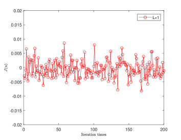
The case $L=1$.

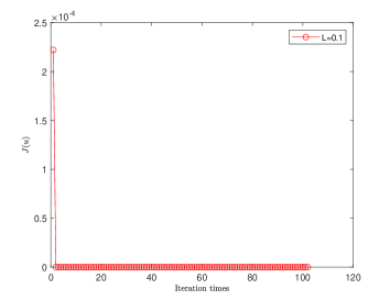
The case $L=0.1$.

Figure 1: The performance of Algorithm 2.2 corresponding to different choices of $L$.

In Figure 1, the graph on the left-hand side indicates that $J(u^{m-1}(\cdot))$ fluctuates up and down around the optimal cost $0$ as $m$ increases. The graph on the right-hand side indicates that $J(u^{0}(\cdot))=2.25\times 10^{-4}$ at the initial time and it descends to the optimal cost $0$ rapidly after one iterative step, and then $J(u^{m-1}(\cdot))$ remains steady at $0$ as $m$ increases. One can note that the convergence is rapid and sharp.

In conclusion, when $L$ is relatively small, Algorithm 2.2 converges to the minimum of Example 4.1 ($L=0.1$). This demonstrates that the modified MSA can indeed help us find the optimum for some simple or specific stochastic recursive control problems. However, it shows some fluctuation of the sequence $\{J(u^{m}(\cdot))\}_{m}$ around the optimal value when we set a relatively larger $L$ ($L=1$). The reason for this phenomenon may involve the error of discretizing the time interval and the computational error of solving the FBSDE in Example 4.1 by the numerical method.

References

- [1] V. G. Boltyanski, R. V. Gamkrelidze and L. S Pontryagin, On the theory of optimal processes. Dokl. Akad. Nauk SSSR, 10 (1956), pp. 7-10.
- [2] R. Carmona, Lectures on BSDEs, Stochastic Control, and Stochastic Differential Games with Financial Applications. Ringgold, Inc, 2016.
- [3] F. L. Chernousko and A. A. Lyubushin, Method of successive approximations for solution of optimal control problems. Optimal Control Applications and Methods, 3 (1982), pp. 101-114.
- [4] F. Delbaen and S. Tang, Harmonic analysis of stochastic equations and backward stochastic differential equations. Probability Theory and Related Fields, 146 (2010), pp. 291-336.
- [5] Duffie, D. and L. Epstein, Stochastic Differential Utility. Econometrica, 60(2) (1992), pp. 353–394.
- [6] M. Fuhrman, Y Hu and G. Tessitore, Stochastic maximum principle for optimal control of SPDEs. Applied Mathematics and Optimization, 68 (2013), pp. 181-217.
- [7] E. Gobet, J-P. Lemor and X. Warin, A regression-based Monte Carlo method to solve backward stochastic differential equations. Annals of Applied Probability, 15 (2005), pp. 2172-2202.
- [8] S. He, J. Wang and J. Yan, Semimartingale Theory and Stochastic Calculus. Science Press, Beijing 1992.
- [9] M. Hu, Stochastic global maximum principle for optimization with recursive utilities. Probability, Uncertainty and Quantitative Risk, 2(1) (2017), pp. 1-20.
- [10] M. Hu, S. Ji and X. Xue, A global stochastic maximum principle for fully coupled forward-backward stochastic systems. SIAM Journal on Control and Optimization, 56(6) (2018), pp. 4309-4335.
- [11] Y. Hu and S. Peng, Solution of forward-backward stochastic differential equations. Probability Theory and Related Fields, 103(2) (1995), pp. 273-283.
- [12] Y. Hu and S. Tang, Multi-dimensional backward stochastic differential equations of diagonally quadratic generators. Stochastic Processes and Their Applications, 126 (2016), pp. 1066-1086.
- [13] E. Hui, J. Huang, X. Li and G. Wang, Near-optimal control for stochastic recursive problems. Systems & Control Letters, 60 (2011), pp. 161-168.
- [14] N. El Karoui, S. Peng and M. C. Quenez, Backward stochastic differential equations in finance. Mathematical Finance, 7(1) (1997), pp. 1-71.
- [15] N. Kazamaki, Continuous exponential martingales and BMO. Springer-Verlag Berlin Heidelberg, 1994.
- [16] B. Kerimkulov, D. Šiška and Ł. Szpruch, A modified MSA for stochastic control problems. Applied Mathematics and Optimization, 84(3) (2021), 3417–3436.
- [17] B. Kerimkulov, D. Šiška and Ł. Szpruch, Exponential convergence and stability of Howard’s policy improvement algorithm for controlled diffusions. SIAM Journal on Control and Optimization, 58(3) (2020), pp. 1314-1340.
- [18] I. A. Krylov and F. L. Chernousko, On the method of successive approximations for solution of optimal control problems. Computational Mathematics and Mathematical Physics, 2(6) (1962), pp. 1371-1382.
- [19] I. A. Krylov and F. L. Chernousko, Algorithm of the method of successive approximations for optimal control problems. Computational Mathematics and Mathematical Physics, 12(1) (1972), pp. 15-38.
- [20] A. Lazrak and M. C. Quenez, A generalized stochastic differential utility. Mathematics of Operations Research, 28(1) (2003), pp. 154-180.
- [21] Q. Li, L. Chen, C. Tai, and W. E, Maximum principle based algorithms for deep learning. Journal of Machine Learning Research, 18(165) (2018), pp. 1-29.
- [22] A. A. Lyubushin, Modifications and convergence investigation of method of successive approximations for optimal control problems. Computational Mathematics and Mathematical Physics, 19(6) (1979), pp. 53-61.
- [23] J. Ma, P. Protter and J. Yong, Solving forward-backward stochastic differential equations explicitly - a 4 step scheme. Probability Theory and Related Fields, 98 (1994), pp. 339-359.
- [24] S. Peng, A general stochastic maximum principle for optimal control problems. SIAM Journal on Control and Optimization, 28(4) (1990), pp. 966-979.
- [25] S. Peng, Backward stochastic differential equations and applications to optimal control. Applied mathematics & optimization, 27(2) (1993), pp. 125-144.
- [26] S. Peng, Open problems on backward stochastic differential equations. Control of Distributed Parameter and Stochastic Systems, 13 (1999), pp. 265-273.
- [27] P. Protter, Stochastic Differential Equations: A New Approach. Springer-Verlag, Berlin, 1990.
- [28] S. Tang, The maximum principle for partially observed optimal control of stochastic differential equations. SIAM Journal on Control and Optimization, 36(5) (1998), pp. 1596–1617.
- [29] S. Tang and X. Li, Necessary conditions for optimal control of stochastic systems with random jumps. SIAM Journal on Control and Optimization, 32(5) (1994), pp. 1447-1475.
- [30] J. Yong and X. Zhou, Stochastic Controls: Hamiltonian Systems and HJB Equations. Springer, 1999.
- [31] J. Zhang, Backward Stochastic Differential Equations: From Linear to Fully Nonlinear Theory (Vol. 86). Springer, New York, 2017.
- [32] X. Zhou, Stochastic near-optimal controls: necessary and sufficient conditions for near-optimality. SIAM Journal on Control and Optimization, 36(3) (1998), pp. 929-947.