​​​​​​​​​​​​​​​ ​​​​​​​​​​

Phenomenological Consequences of Supersymmetric Theories from Dimensional Reduction and Reduction of Couplings
PhD Thesis of
GREGORY PATELLIS
Department of Physics
National Technical University of Athens

SUPERVISOR:
George Zoupanos
Professor Emeritus NTUA

December 2020

​​​​​​​​​​​​​​​ ​​​​​​​​​​ ΕΘΝΙΚΟ ΜΕΤΣΟΒΙΟ ΠΟΛϒΤΕΧΝΕΙΟ
ΣΧΟΛΗ ΕΦΑΡΜΟΣΜΕΝΩΝ ΜΑΘΗΜΑΤΙΚΩΝ
ΚΑΙ ΦϒΣΙΚΩΝ ΕΠΙΣΤΗΜΩΝ

Phenomenological Consequences of Supersymmetric Theories from Dimensional Reduction and Reduction of Couplings
PhD Thesis of
GREGORY PATELLIS
Department of Physics
National Technical University of Athens

3-MEMBER ADVISORY COMMITTEE:

1………….George Koutsoumbas, Prof. NTUA
2………….Nicholas Tracas, Prof. NTUA
3………….George Zoupanos, Prof. Emer. NTUA
3………….(Supervisor)
l

7-MEMBER EXAMINING COMMITTEE:

1…………Konstantinos Anagnostopoulos,
4…………Assoc. Prof. NTUA
2…………Konstantinos Farakos, Prof. NTUA
3…………Nikos Irges, Assoc. Prof. NTUA
4…………George Koutsoumbas, Prof. NTUA
5…………George Leontaris, Professor UOI
6…………Myriam Mondragón, Prof. UNAM
7…………Nicholas Tracas, Prof. NTUA

Athens, December 2020

a

“Man can will nothing unless he has first understood that he must
count on no one but himself; that he is alone, abandoned on earth in the
midst of his infinite responsibilities, without help, with no other aim than the one
he sets himself, with no other destiny than the one he forges for himself on this earth.”
JP. S.

Ευχαριςτιες

Καταρχας, ϑα ηϑελα να ευχαριςτηςω απο ϰαρδιας τον επιβλεποντα µου, Οµ. Καϑηγητη Γιωργο Ζουπανο, για την ϰαϑοδηγηςη του ολοϰληρη την τελευταια δεϰαετια. Στο επιςτηµονιϰο ϰοµµατι, µεταξυ πολλων αλλων, για την -αµεςη η εµµεςη- προτροπη ςτη ςφαιριϰη ϰατανοηςη αντι της εµµονης ςτο υπερ του δεοντος ςυγϰεϰριµενο. Κυριως οµως για την ςπανια ηϑιϰη του αϰεραιοτητα ςε ϰαϑε τοµεα, επιςτηµονιϰο ϰαι ϰοινωνιϰο. Τον ευχαριςτω επιςης για την δυνατοτητα ςυµµετοχης -αλλα ϰαι ςυνειςφορας- που µου εδωςε ςτο ετηςιο διεϑνες ςυνεδριο της Κερϰυρας, αλλα ϰαι για την ενϑαρρυνςη για επιςϰεψεις ςε διαϰεϰριµενα ιδρυµατα του εξωτεριϰου, ςτα οποια βρηϰα ςυνεργατες διεϑνους δραςτηριοτητας ϰαι αναγνωριςης.

Θα ηϑελα να ευχαριςτηςω τους δυο ςυνεργατες µου, την Καϑηγητρια Myriam Mondragón ϰαι τον Καϑηγητη Sven Heinemeyer, για την πολυτιµη βοηϑεια ϰαι τις ςυµβουλες που µου προςεφεραν ϰαϑολη τη διαρϰεια της ςυνεργαςιας µας.

Επιςης, ευχαριςτω τους ςυνεπιβλεποντες µου, τον Καϑηγητη Νιϰολα Τραϰα ϰαι τον Καϑηγητη Γιωργο Κουτςουµπα, ϰαϑως ηταν παντα προϑυµοι να απαντηςουν ςε ϰαϑε µου ερωτηςη, αλλα ϰαι τον ςτενο µου φιλο ϰαι ςυνεργατη, Γιωργο Μανωλαϰο, διοτι, περα απο τη βοηϑεια του ςε επιςτηµονιϰο επιπεδο, αντεξε ολα µου τα παραπονα τον τελευταιο ϰαιρο.

Αϰοµα, ευχαριςτω ολους τους ϰαλους φιλους που απεϰτηςα αυτα τα χρονια, πανεπιςτηµιαϰους ϰαι χορευτιϰους, ϰαϑως η παρεα ϰαι οι ςυζητηςεις µαζι τους διαµορφωςαν ςε µεγαλο βαϑµο το πλαιςιο µεςα ςτο οποιο η προςπαϑεια µου αυτη αποϰτα νοηµα.

Τελος, δε γινεται να µην αφιερωςω την παρουςα διατριβη ςτη µητερα µου ϰαι τη γιαγια µου, χωρις την αϰουραςτη ςτηριξη των οποιων δε ϑα ηταν δυνατο να ολοϰληρωϑει.

Περιληψη

Η ιδεα της «ελαττωςης παραµετρων» βαςιζεται ςτην ευρεςη ςχεςεων αναλλοιωτων ϰατω απο την οµαδα επαναϰανονιϰοποιηςης µεταξυ παραµετρων µιας επαναϰανονιϰοποιηςιµης ϑεωριας, οι οποιες ιςχυουν ςε ολες τις ταξεις ϑεωριας διαταραχων. Αυτη η µεϑοδος µπορει να εφαρµοςτει ςε $N=1$ υπερςυµµετριϰες ϑεωριες µεγαλης ενοποιηςης, ϰαϑιςτωντας τις πεπεραςµενες ςε ϰαϑε επιπεδο βροχων. Στο πρωτο µερος της παρουςας διατριβης, µετα απο ςυντοµη αναδροµη ςτις βαςιϰες αρχες της ελαττωςης παραµετρων ϰαι της περατοτητας, εξεταζονται τεςςερα µοντελα που παρουςιαζουν µεγαλο φαινοµενολογιϰο ενδιαφερον: µια ελαχιςτοποιηµενη εϰδοχη του $N=1$ υπερςυµµετριϰου µοντελου $SU(5)$, το πεπεραςµενο $N=1$ υπερςυµµετριϰο µοντελο $SU(5)$, το πεπεραςµενο (ςε επιπεδο δυο βροχων) $N=1$ υπερςυµµετριϰο µοντελο $SU(3)\otimes SU(3)\otimes SU(3)$ ϰαι µια ελαχιςτοποιηµενη εϰδοχη του Ελαχιςτου ϒπερςυµµετριϰου Καϑιερωµενου Προτυπου (ΕϒΚΠ). Η επανεξεταςη αυτων των µοντελων παρουςιαζει µια βελτιωµενη τιµη της µαζας του ελαφρου ςωµατιδιου Higgs, οπου για την αναλυςη χρηςιµοποιηϑηϰε η ϰαινουρια εϰδοχη του προγραµµατος FeynHiggs. Το ελαφρυτερο υπερςυµµετριϰο ςωµατιδιο, εφοςον ειναι neutralino, µπορει να ϑεωρηϑει ως υποψηφιο ςωµατιδιο ςϰοτεινης υλης, υποϑεςη που εξεταζεται µε το προγραµµα MicrOMEGAs, αν ϰαι ϰανενα µοντελο δεν δινει ιϰανοποιητιϰα αποτελεςµατα ςε αυτην την ϰατευϑυνςη. Στα τρια ενοποιηµενα µοντελα παρατηρουνται ςχετιϰα βαρια υπερςυµµετριϰα φαςµατα (τα οποια παρηχϑηςαν µε τα προγραµµατα FeynHiggs ϰαι SPheno) που ξεϰινουν πανω απο το $1\leavevmode\nobreak\ TeV$, οποτε ειναι ςυνεπη µε την µη παρατηρηςη τους απο τον Μεγαλο Επιταχυντη Αδρονιων (LHC), ενω το ελαχιςτοποιηµενο ΕϒΚΠ παρουςιαζει τη µαζα του ψευδοβαϑµωτου µποζονιου Higgs, $M_{A}$, ςε περιοχη που αποϰλειεται απο προςφατα αποτελεςµατα του πειραµατος ATLAS. Η δυνατοτητα αναϰαλυψης ϰαϑενος απο τα τρια µοντελα ενοποιηςης ςτον HL-LHC ειναι µηδαµινη, οµως ο FCC-hh πιςτευεται οτι ϑα ειναι ςε ϑεςη να παρατηρηςει µεγαλο µερος των φαςµατων των τριων µοντελων.

Στο δευτερο µερος της διατριβης, µετα απο µια αναδροµη ςτις βαςιϰες εννοιες της Διαςτατιϰης Ελαττωςης ςε Χωρους Πηλιϰου, παρουςιαζεται µια επεϰταςη του Καϑιερωµενου Προτυπου, η οποια προϰυπτει απο τη διαςτατιϰη ελαττωςη µιας $N=1$, $10D$ $E_{8}$ ϑεωριας ςε ενα χωρο της µορφης $M_{4}\times B_{0}/\mathbf{Z}_{3}$, οπου $B_{0}$ ειναι η nearly-Kähler πολλαπλοτητα $SU(3)/U(1)\times U(1)$ ϰαι $\mathbf{Z}_{3}$ ειναι µια ”freely-acting” διαϰριτη ςυµµετρια του $B_{0}$. Η εφαρµογη του µηχανιςµου ςπαςιµατος Wilson flux ϰαταληγει ςε µια $N=1$ ϑεωρια βαϑµιδας $SU(3)^{3}$, µε δυο επιπλεον ϰαϑολιϰες ςυµµετριες $U(1)$. Κατω απο την ϰλιµαϰα ενοποιηςης εχουµε ενα µοντελο µε δυο διπλετες Higgs ςε µια split-like υπερςυµµετριϰη εϰδοχη του Καϑιερωµενου Προτυπου η οποια ειναι φαινοµενολογιϰα ςυνεπης, εφοςον παραγει µαζες για το µποζονιο Higgs ϰαι τα ϰουαρϰς της τριτης οιϰογενειας ςε ςυµφωνια µε τις προςφατες πειραµατιϰες µετρηςεις, ενω η τιµη της µαζας του ελαφρυτερου υπερςυµµετριϰου ςωµατιδιου προβλεπεται ςτα $\sim 1500\leavevmode\nobreak\ GeV$.

Abstract

The ’reduction of couplings’ idea consists in the search for renormalization group invariant (RGI) relations between seemingly independent parameters of a renormalizable theory that hold to all orders of perturbation theory. This concept can be applied to $N=1$ supersymmetric Grand Unified Theories (GUTs) and make them finite at all loops. In the first part of this thesis, after a review of the reduction of couplings method and the properties of the resulting finiteness in supersymmetric theories, four phenomenologically interesting models are analysed: a minimal version of the $N=1$ supersymmetric $SU(5)$, a finite $N=1$ supersymmmetric $SU(5)$, a two-loop finite $N=1$ supersymmetric $SU(3)\otimes SU(3)\otimes SU(3)$ model and a reduced version of the Minimal Supersymmetric Standard Model (MSSM). A relevant update in the phenomenological evaluation has been the improved light Higgs-boson mass prediction as provided by the latest version of FeynHiggs. The lightest supersymmetric particle (LSP), which is a neutralino, is considered as a cold dark matter (CDM) candidate and put to test using the latest MicrOMEGAs code, although no model supports an acceptable value of the CDM relic density. The first three models predict relatively heavy supersymmetric spectra (produced using the FeynHiggs and SPheno codes) that start just above the TeV scale, consistent with the non-observation LHC results, while the reduced MSSM results in a pseudoscalar Higgs boson mass $M_{A}$ that is ruled out by recent results of the ATLAS experiment. The prospects of discovery of the three models at the HL-LHC vary from very dim to none, depending on the model. The FCC-hh, however, will in principle be able to test large parts of the predicted spectrum of each unified model.

In the second part of the thesis, after a review of the Coset Space Dimensional Reduction (CSDR) scheme, an extension of the Standard Model is presented that results from the dimensional reduction of the $N=1$, $10D$ $E_{8}$ group over a $M_{4}\times B_{0}/\mathbf{Z}_{3}$ space, where $B_{0}$ is the nearly-Kähler manifold $SU(3)/U(1)\times U(1)$ and $\mathbf{Z}_{3}$ is a freely acting discrete group on $B_{0}$. Using the Wilson flux breaking mechanism we are left in four dimensions with an $N=1$ $SU(3)^{3}$ gauge theory plus two global $U(1)$s. Below the unification scale we have a two Higgs doublet model in a split-like supersymmetric version of the Standard Model which is phenomenologically consistent, since it produces masses of a light Higgs, the top and the bottom particles within the experimental limits and predicts the LSP $\sim 1500\leavevmode\nobreak\ GeV$.

Contents

1. 1 Introduction
2. I Theories with Reduced Couplings - Finite Theories
   1. 2 Reduction of Couplings
      1. 2.1 Reduction of Dimensionless Parameters
      2. 2.2 Reduction of Couplings in $N=1$ SUSY Gauge Theories - Partial Reduction
      3. 2.3 Reduction of Dimension-1 and -2 Parameters
      4. 2.4 Reduction of Couplings of Soft Breaking Terms in $N=1$ SUSY Theories
   2. 3 Finiteness
      1. 3.1 The idea behind finiteness
      2. 3.2 Finiteness in N=1 Supersymmetric Gauge Theories
   3. 4 Phenomenologically Interesting Models with Reduced Couplings
      1. 4.1 The Minimal $N=1$ Supersymmetric $SU(5)$
      2. 4.2 The Finite $N=1$ Supersymmetric $SU(5)$
      3. 4.3 Finite $SU(N)^{3}$ Unification
      4. 4.4 Reduction of Couplings in the MSSM
   4. 5 Analysis of Phenomenologically Viable Models
      1. 5.1 Phenomenological Constraints
      2. 5.2 Computational setup
      3. 5.3 The Minimal $N=1$ $SU(5)$
      4. 5.4 The Finite $N=1$ $SU(5)$
      5. 5.5 The Two-Loop Finite $N=1$ $SU(3)\otimes SU(3)\otimes SU(3)$
      6. 5.6 The Reduced MSSM
3. II Trinification from Coset Space Dimensional Reduction
   1. 6 The Coset Space Dimensional Reduction
      1. 6.1 Coset Space Geometry
      2. 6.2 Main Features and Constraints of CSDR
      3. 6.3 The action of the reduced four-dimensional theory
      4. 6.4 CSDR and the Einstein-Yang-Mills Theory
   2. 7 Dimensional Reduction of $E_{8}$ over $SU(3)/U(1)\times U(1)$
   3. 8 Wilson Flux Breaking
      1. 8.1 Wilson Flux basics
      2. 8.2 $SU(3)^{3}$ produced by Wilson Flux
   4. 9 Selection of Parameters and GUT breaking
      1. 9.1 Choice of radii
      2. 9.2 Further gauge symmetry breaking of $SU(3)^{3}$
      3. 9.3 Electroweak Currents and $\sin{\theta_{W}}$
      4. 9.4 Lepton Yukawa couplings and $\mu$ terms
   5. 10 Phenomenological Analysis of $SU(3)^{3}$ with Small Coset Space Radii
      1. 10.1 Constraints
      2. 10.2 Gauge unification
      3. 10.3 Higgs potential
      4. 10.4 1-loop results
   6. 11 Conclusions
   7. A Reducing the 10-dimensional 32-spinor to 8-spinor by Majorana-Weyl Condition
   8. B Useful relations for the gaugino mass calculation
   9. C Calculation of $D^{A}$ terms
   10. D Calculation of scalar potential terms
   11. E Trinification supersymmetry breaking terms at the vacuum
   12. F Analytical expressions for $\beta$ functions

Chapter 1 Introduction

An essential direction of the theoretical efforts of the last decades in Elementary Particle Physics (EPP) is to understand the free parameters of the Standard Model (SM) in terms of few fundamental ones, i.e. to achieve reductions of couplings[1]. However, despite the many successes of the SM in describing elementary particles and their interactions, there is little to no progress when it comes to the plethora of free parameters. The pathology of the large number of free parameters is deeply correlated to the infinities that emerge at the quantum level. Renormalization removes the infinities, but only at the cost of introducing counterterms that add to the number of free parameters.

Although the SM is a successful theory, the widespread belief suggests that it will be proven to be the low energy limit of a fundamental theory. The search for physics beyond the Standard Model (BSM) expands in various directions. One of the most efficient ways to reduce the number of free parameters of a theory (and thus render it more predictive) is the introduction of a symmetry. A celebrated application of such an idea are the Grand Unified Theories (GUTs) [2, 3, 4, 5, 6, 7]. Decades ago, an early version of $SU(5)$ reduced the gauge couplings of the SM (featuring an -approximate- gauge unification), predicting one of them. It was the addition of an $N=1$ (softly broken) supersymmetry (SUSY) [8, 9, 10] that made the prediction viable. In the framework of GUTs, the Yukawa couplings can also be related among themselves. Again, $SU(5)$ demonstrated this by predicting the ratio of the tau to bottom mass [11] for the SM. Unfortunately, the introduction of additional gauge symmetry does not seem to help, since new complications arise due to new degrees of freedom, i.e. the channels of breaking the symmetry.

An alternative way to look for relations among seemingly unrelated parameters is the reduction of couplings method [12, 13, 14] (see also refs [15, 16, 17]). This technique reduces the number of parameters of a theory by relating either all or a number of couplings to a single parameter, the “primary coupling”. This method can identify hidden symmetries in a system, but it is also possible to have reduction of couplings in systems with no apparent symmetry. It is necessary, though, to make two assumptions: both the original and the reduced theory have to be renormalizable and the relations among parameters should be Renormalization Group Invariant (RGI).

A natural extension of the idea of Grand Unification is to achieve gauge-Yukawa Unification (GYU), that is to relate the gauge sector to the Yukawa sector. This is a feature of theories in which reduction of couplings has been applied. The original suggestion for the reduction of couplings in GUTs leads to the search for RGI relations that hold below the Planck scale, which are in turn preserved down to the unification scale. Impressively, this observation guarantees validity of such relations to all-orders in perturbation theory. This is done by studying their uniqueness at one-loop level. Even more remarkably, one can find such RGI relations that result in all-loop finiteness. The above principles have only been applied in $N=1$ supersymmetric GUTs for reasons that will be transparent in the following chapters. The application of the GYU programme in the dimensionless couplings of such theories has been very successful, including the prediction of the mass of the top quark in the minimal [18] (see also Chapter 5 for the latest update) and in the finite $N=1$ $SU(5)$ [19, 20] before its experimental discovery [21].

In order to successfully apply the above-mentioned programme, SUSY appears to be essential. However, one has to understand its breaking as well, since it has the ambition to supply the SM with predictions for several of its free parameters. Indeed, the search for RGI relations has been extended to the soft supersymmetry breaking sector (SSB) of these theories, which involves parameters of dimension one and two. In addition, there was important progress concerning the renormalization properties of the SSB parameters, based on the powerful supergraph method for studying supersymmetric theories, and it was applied to the softly broken ones by using the“spurion” external space-time independent superfields. According to this method a softly broken supersymmetric gauge theory is considered as a supersymmetric one in which the various parameters, such as couplings and masses, have been promoted to external superfields. Then, relations among the soft term renormalization and that of an unbroken supersymmetric theory have been derived. In particular the $\beta$-functions of the parameters of the softly broken theory are expressed in terms of partial differential operators involving the dimensionless parameters of the unbroken theory. The key point in solving the set of coupled differential equations so as to be able to express all parameters in a RGI way, was to transform the partial differential operators involved to total derivative operators. It is indeed possible to do this by choosing a suitable RGI surface.

The application of reduction of couplings on $N=1$ SUSY theories has led to many interesting phenomenological developments, too. In past work, an appealing “universal” set of soft scalar masses was assumed in the SSB sector of supersymmetric theories, given that apart from economy and simplicity (1) they are part of the constraints that preserve finiteness up to two loops, (2) they appear in the attractive dilaton dominated supersymmetry breaking superstring scenarios. However, further studies have exhibited a number of problems, all due to the restrictive nature of the “universality” assumption for the soft scalar masses. Subsequently, this constraint was replaced by a more “relaxed” all-loop RGI soft scalar squared masses sum rule that keeps the most attractive features of the universal case and overcomes the unpleasant phenomenological consequences. This arsenal of tools and results opened the way for the study of full finite models with few free parameters, with emphasis given on predictions for the SUSY spectrum and the light Higgs boson mass.

The Higgs mass prediction, which coincided with the LHC results (ATLAS [22, 23] and CMS [24, 25]) - combined with a predicted relatively heavy spectrum of SUSY particles - was a success of the all-loop finite $N=1$ SUSY $SU(5)$ model [26], while another finite theory, namely the $N=1$ (two-loop) finite $SU(3)\otimes SU(3)\otimes SU(3)$ [27] (see also [28, 29] for alternative versions of the model), also confirmed the LHC results. Additionally, the above programme was also applied in the MSSM [30, 31], with successful results concerning the top, bottom and Higgs masses, also featuring a relatively heavy SUSY spectrum (a review of past analyses can be found in [32]). Furthermore, it is a well known fact that the lightest neutralino, being the Lightest SUSY Particle (LSP), is an excellent candidate for Cold Dark Matter (CDM) [33].

On the other hand, apart from the efforts to reduce the arbitrariness in our description of Nature, the unification of all fundamental interactions has been - for more than half a century- the theoretical physicists’ desideratum. The community sets this direction in high priority, and as a result several interesting approaches have been developed over the past decades. Out of all of them, the ones that support and/or employ the existence of extra dimensions are perhaps the most prominent. The extra-dimensional scenarios are encouraged by a very consistent framework, the superstring theories [34], with the most promising being the heterotic string [35] (defined  in ten dimensions), due to its potential experimental testability. Specifically, the phenomenological aspect of the heterotic string is designated in the resulting GUTs, containing the SM gauge group, which are obtained after compactifying the 10D spacetime and performing a dimensional reduction of the $E_{8}\times E_{8}$ initial gauge theory. In addition, a few years before the formulation of superstring theories, an alternative framework of dimensional reduction of higher-dimensional gauge theories emerged. This important undertaking, which shared common aims with one of the many superstring theories, was initially explored by Forgacs-Manton (F-M) and Scherk-Schwartz (S-S) studying the Coset Space Dimensional Reduction (CSDR) [36, 37, 38] and the group manifold reduction [39], respectively.

In the higher-dimensional theory, the gauge fields unify the gauge and scalar sector, while, after the dimensional reduction, the resulting 4D theory features a particle spectrum of the surviving components. This holds for both approaches (F-M and S-S). Moreover, in the CSDR programme, inclusion of fermions in the higher-dimensional theory gives rise to Yukawa interactions in the resulting 4D theory. Furthermore, for a specific choice of initial dimensions, one can unify the fields even more if the higher-dimensional gauge theory is $N=1$ supersymmetric, in the way that both gauge and fermionic fields are accommodated in the same vector supermultiplet. It is important to note that the CSDR scheme allows the possibility of obtaining chiral 4D theories [40, 41].

In the CSDR context, some notions inspired from the heterotic string were incorporated, specifically the dimensionality of the spacetime and the gauge group of the higher-dimensional theory. Therefore, taking into consideration that superstring theories are consistent in ten dimensions, the extra dimensions have to be distinguished from the four observable ones with a compactification of the metric and then the resulting 4D theory is determined. Furthermore, a suitable choice of compactification manifold can lead to 4D, $N=1$ supersymmetric theories, aiming for realistic GUTs.

When dimensionally reducing an $N=1$ supersymmetric gauge theory, a very important and desired property is the amount of supersymmetry of the initial theory to be preserved in the 4D one. Some very good candidates that preserve it are the compact internal Calabi–Yau (CY) manifolds [42]. However, the moduli stabilization problem that emerges led to the study of flux compactification in a wider class of internal spaces, namely manifolds with an SU(3)-structure. In these manifolds a background non-vanishing, globally defined spinor is considered. This spinor is covariantly constant with respect to a connection including torsion, while, in the CY case, this holds for a Levi–Civita connection. Here, the nearly-Kähler manifolds class of the SU(3)-structure manifolds is considered [43, 44, 45, 46] , [47, 48, 49], [50, 51, 52, 53] , [54, 55, 56] , [57, 58, 59, 60, 61, 62, 63, 64, 65]. Specifically, the class of 6D homogeneous nearly-Kähler manifolds includes the non-symmetric coset spaces $G_{2}/SU(3)$, $Sp(4)/SU(2)\times U(1)_{non-max}$, $SU(3)/U(1)\times U(1)$ and the group manifold $SU(2)\times SU(2)$ [65] (see also [43, 44, 45, 46, 47, 48, 49, 50, 51, 52, 53, 54, 55, 56, 57, 58, 59, 60, 61, 62, 63, 64]). It is worth mentioning that, contrary to the CY case, the dimensional reduction of a 10D $N=1$ supersymmetric gauge theory over a non-symmetric coset space, leads to 4D theories which include supersymmetry breaking terms [66, 67, 68].

The above-mentioned framework has a very interesting application in the dimensional reduction of an $N-1$, 10D $E_{8}$ over the compactification space $SU(3)/U(1)\times U(1)\times\mathbf{Z}_{3}$, where the latter is the non-symmetric coset space $SU(3)/U(1)\times U(1)$ equipped with the freely-acting discrete symmetry $Z_{3}$. This extra symmetry is needed in order to employ the Wilson flux breaking mechanism ([69, 70, 71]) to further reduce the gauge symmetry of the $4D$ GUT. Specifically, the $E_{6}$ GUT (along with two $U(1)$ global symmetries) is broken to the trinification group, $SU(3)^{3}$ [37, 66, 54, 63] (see also [72]). The potential of the resulting 4D theory contains terms that can be identified as $F$-, $D$- and soft breaking terms, which means that the resulting theory is a (broken) $N=1$ supersymmetric theory.

The present thesis in organised as follows:
Starting from Part I, in Chapter 2 there is a brief review of the reduction of couplings principle and method. In Chapter 3 the notion of finiteness is explained and the way to obtain finite theories with dimensionless and dimensionful couplings is reviewed. Chapter 4 reviews four phenomenologically promising models, namely the Minimal $N=1$ $SU(5)$, the all-loop Finite $N=1$ $SU(5)$, the two-loop Finite $SU(3)\otimes SU(3)\otimes SU(3)$ and the Reduced MSSM. Their analysis follows in Chapter 5 (see the original publications [73, 74, 75]). Our analyses predict the top, bottom and light Higgs masses within experimental limits (with the exception of the bottom mass in the Minimal $SU(5)$ model), produce the full supersymmetric spectrum and the SUSY breaking scale, the CDM relic density for the LSP and the cross sections and branching rations necessary to determine the discovery potential of each model in (near) future colliders. While our analysis is based on the Higgs sector results obtained with the new version of FeynHiggs 2.16.0 code [76, 77, 78, 79], other software was used as well. In particular, SPheno 4.0.4 [80, 81] was used for the calculation of branching ratios, MadGraph [82] for the calculation of the cross sections and the MicrOMEGAs 5.0 [83, 84, 85] code was used for the calculation of the CDM relic density. As will be discussed in Chapter 5, none of the models satisfy the experimental bounds of the relic density.

Proceeding to Part II, Chapter 6 reviews the CSDR scheme and the reduction of a $D$-dimensional Yang-Mills-Dirac theory accordingly. In Chapter 7 the application of the CSDR programme in the case of a $N=1$, $10D$ $E_{8}$ group reduced over the non-symmetric coset $SU(3)/U(1)\times U(1)$ in demonstrated. The necessary Wilson flux breaking using a $Z_{3}$ discrete symmetry is demonstrated in Chapter 8 and the $SU(3)^{3}$ GUT is obtained. The radii of the coset are chosen to be small in a specific configuration, while the compactification and unification scales coincide, leading to a split-like supersymmetry scenario in which some supersymmetric particles are superheavy and others obtain mass in the $TeV$ region, as described in Chapter 9. After the employment of the spontaneous symmetry breaking of the GUT, the model can be viewed as a two Higgs doublet model (2HDM). The detailed phenomenological analysis of the model is presented in Chapter 10 (see [86] for the original work). Finally, some closing remarks can be found in 11.

Part I Theories with Reduced Couplings - Finite Theories

Chapter 2 Reduction of Couplings

The basic idea of reduction of couplings should be the first to be reviewed, as first introduced in [12] and consequently evolved and expanded over the next two decades. The aim is to express the parameters of a theory that are considered free in terms of one basic parameter called primary coupling. The basic idea is to search for RGI relations among couplings and use them to reduce the seemingly independent parameters. It is first applied to parameters without mass dimension, then extended to parameters of dimension one or two, i.e. the couplings and masses of the soft breaking sector of an $N=1$ supersymmetric theory.

2.1 Reduction of Dimensionless Parameters

Any RGI relation (i.e. which does not depend on the renormalization scale $\mu$ explicitly) among couplings $g_{1},...,g_{A}$ of a given renormalizable theory can be expressed in the implicit form $\Phi(g_{1},\cdots,g_{A})\leavevmode\nobreak\ =\leavevmode\nobreak\ \mbox{const.}$, which has to satisfy the  partial differential equation (PDE)

$$\mu\,\frac{d\Phi}{d\mu}={\vec{\nabla}}\Phi\cdot{\vec{\beta}}\leavevmode\nobreak\ =\leavevmode\nobreak\ \sum_{a=1}^{A}\,\beta_{a}\,\frac{\partial\Phi}{\partial g_{a}}\leavevmode\nobreak\ =\leavevmode\nobreak\ 0\leavevmode\nobreak\ ,$$ (2.1)

where $\beta_{a}$ is the $\beta$-function of $g_{a}$. Solving this PDE is equivalent to solving a set of ordinary differential equations, the so-called reduction equations (REs) [12, 13, 14],

$$\beta_{g}\,\frac{dg_{a}}{dg}=\beta_{a}\leavevmode\nobreak\ ,\leavevmode\nobreak\ a=1,\cdots,A\leavevmode\nobreak\ ,$$ (2.2)

where $g$ and $\beta_{g}$ are the primary coupling and its $\beta$-function, respectively, and the counting on $a$ does not include $g$. Since maximally ($A-1$) independent RGI “constraints” in the $A$-dimensional space of couplings can be imposed by the $\Phi_{a}$’s, one could in principle express all the couplings in terms of a single coupling $g$. However, a closer look to the set of Eqs. (2.2) reveals that their general solutions contain as many integration constants as the number of equations themselves. Thus, using such integration constants we have just traded an integration constant for each ordinary renormalized coupling, and consequently, these general solutions cannot be considered as reduced ones. The crucial requirement in the search for RGE relations is to demand power series solutions to the REs,

$$g_{a}=\sum_{n}\rho_{a}^{(n)}\,g^{2n+1}\leavevmode\nobreak\ ,$$ (2.3)

which preserve perturbative renormalizability. Such an ansatz fixes the corresponding integration constant in each of the REs and picks up a special solution out of the general one. Remarkably, the uniqueness of such power series solutions can be decided already at the one-loop level [12, 13, 14]. To illustrate this, we may assume $\beta$-functions of the form

$$\begin{split}\beta_{a}&=\frac{1}{16\pi^{2}}\left[\sum_{b,c,d\neq g}\beta^{(1)\,bcd}_{a}g_{b}g_{c}g_{d}+\sum_{b\neq g}\beta^{(1)\,b}_{a}g_{b}g^{2}\right]+\cdots\leavevmode\nobreak\ ,\\ \beta_{g}&=\frac{1}{16\pi^{2}}\beta^{(1)}_{g}g^{3}+\cdots\leavevmode\nobreak\ .\end{split}$$ (2.4)

Here $\cdots$ stands for higher-order terms, and $\beta^{(1)\,bcd}_{a}$’s are symmetric in $b,c,d$. We then assume that the $\rho_{a}^{(n)}$’s with $n\leq r$ have been uniquely determined. To obtain $\rho_{a}^{(r+1)}$’s, we insert the power series (2.3) into the REs (2.2) and collect terms of ${\cal O}(g^{2r+3})$. Thus, we find

$$\sum_{d\neq g}M(r)_{a}^{d}\,\rho_{d}^{(r+1)}=\mbox{lower order\leavevmode\nobreak\ quantities}\leavevmode\nobreak\ ,$$

where the right-hand side is known by assumption and

$$M(r)_{a}^{d} =3\sum_{b,c\neq g}\,\beta^{(1)\,bcd}_{a}\,\rho_{b}^{(1)}\,\rho_{c}^{(1)}+\beta^{(1)\,d}_{a}-(2r+1)\,\beta^{(1)}_{g}\,\delta_{a}^{d}\leavevmode\nobreak\ ,$$ (2.5)

$$0 =\sum_{b,c,d\neq g}\,\beta^{(1)\,bcd}_{a}\,\rho_{b}^{(1)}\,\rho_{c}^{(1)}\,\rho_{d}^{(1)}+\sum_{d\neq g}\beta^{(1)\,d}_{a}\,\rho_{d}^{(1)}-\beta^{(1)}_{g}\,\rho_{a}^{(1)}\leavevmode\nobreak\ .$$ (2.6)

Therefore, the $\rho_{a}^{(n)}$’s for all $n>1$ for a given set of $\rho_{a}^{(1)}$’s can be uniquely determined if $\det M(n)_{a}^{d}\neq 0$ for all $n\geq 0$. This is checked in all models that reduction of couplings is applied.

The various couplings in supersymmetric theories have the same asymptotic behaviour. Therefore, searching for a power series solution of the form (2.3) to the REs (2.2) is justified.

The possibility of coupling unification described in this section is without any doubt very attractive because the “completely reduced” theory contains only one independent coupling, but it can be unrealistic. Therefore, one often would like to impose fewer RGI constraints, and this is the idea of partial reduction [87, 88].

All the above give rise to hints towards an underlying connection among the requirement of reduction of couplings and SUSY. As an example, one can consider a $SU(N)$ gauge theory with $\phi^{i}({\bf N})$ and $\hat{\phi}_{i}(\overline{\bf N})$ complex scalars, $\psi^{i}({\bf N})$ and $\hat{\psi}_{i}(\overline{\bf N})$ left-handed Weyl spinors and $\lambda^{a}\leavevmode\nobreak\ (a=1,\dots,N^{2}-1)$ right-handed Weyl spinors in the adjoint representation of $SU(N)$.

The Lagrangian (kinetic terms are omitted) includes

$${\cal L}\supset i\sqrt{2}\{\leavevmode\nobreak\ g_{Y}\overline{\psi}\lambda^{a}T^{a}\phi-\hat{g}_{Y}\overline{\hat{\psi}}\lambda^{a}T^{a}\hat{\phi}+\mbox{h.c.}\leavevmode\nobreak\ \}-V(\phi,\overline{\phi}),$$ (2.7)

where

$$V(\phi,\overline{\phi})=\frac{1}{4}\lambda_{1}(\phi^{i}\phi^{*}_{i})^{2}+\frac{1}{4}\lambda_{2}(\hat{\phi}_{i}\hat{\phi}^{*\leavevmode\nobreak\ i})^{2}+\lambda_{3}(\phi^{i}\phi^{*}_{i})(\hat{\phi}_{j}\hat{\phi}^{*\leavevmode\nobreak\ j})+\lambda_{4}(\phi^{i}\phi^{*}_{j})(\hat{\phi}_{i}\hat{\phi}^{*\leavevmode\nobreak\ j}),$$ (2.8)

This is the most general renormalizable form in four dimensions. In search of a solution of the form of Eq. (2.3) for the REs, among other solutions, one finds in lowest order:

$$\begin{split}g_{Y}&=\hat{g}_{Y}=g\leavevmode\nobreak\ ,\\ \lambda_{1}&=\lambda_{2}=\frac{N-1}{N}g^{2}\leavevmode\nobreak\ ,\\ \lambda_{3}&=\frac{1}{2N}g^{2}\leavevmode\nobreak\ ,\leavevmode\nobreak\ \lambda_{4}=-\frac{1}{2}g^{2}\leavevmode\nobreak\ ,\end{split}$$ (2.9)

which corresponds to a $N=1$ SUSY gauge theory. While these remarks do not provide an answer about the relation of reduction of couplings and SUSY, they certainly point to further study in that direction.

2.2 Reduction of Couplings in $N=1$ SUSY Gauge Theories - Partial Reduction

Consider a chiral, anomaly-free, $N=1$ globally supersymmetric gauge theory that is based on a group G and has gauge coupling $g$. The superpotential of the theory is:

$$W = \frac{1}{2}\,m_{ij}\,\phi_{i}\,\phi_{j}+\frac{1}{6}\,C_{ijk}\,\phi_{i}\,\phi_{j}\,\phi_{k}\leavevmode\nobreak\ ,$$ (2.10)

where $m_{ij}$ and $C_{ijk}$ are gauge invariant tensors and the chiral superfield $\phi_{i}$ belongs to the irreducible representation $R_{i}$ of the gauge group. The renormalization constants associated with the superpotential, for preserved SUSY, are:

$$\phi_{i}^{0} =\left(Z^{j}_{i}\right)^{(1/2)}\,\phi_{j}\leavevmode\nobreak\ ,\leavevmode\nobreak\$$ (2.11)

$$m_{ij}^{0} =Z^{i^{\prime}j^{\prime}}_{ij}\,m_{i^{\prime}j^{\prime}}\leavevmode\nobreak\ ,\leavevmode\nobreak\$$ (2.12)

$$C_{ijk}^{0} =Z^{i^{\prime}j^{\prime}k^{\prime}}_{ijk}\,C_{i^{\prime}j^{\prime}k^{\prime}}\leavevmode\nobreak\ .$$ (2.13)

By virtue of the $N=1$ non-renormalization theorem [89, 90, 91, 92] there are no mass and cubic interaction term infinities. Therefore:

$$\begin{split}Z_{ij}^{i^{\prime}j^{\prime}}\left(Z^{i^{\prime\prime}}_{i^{\prime}}\right)^{(1/2)}\left(Z^{j^{\prime\prime}}_{j^{\prime}}\right)^{(1/2)}&=\delta_{(i}^{i^{\prime\prime}}\,\delta_{j)}^{j^{\prime\prime}}\leavevmode\nobreak\ ,\\ Z_{ijk}^{i^{\prime}j^{\prime}k^{\prime}}\left(Z^{i^{\prime\prime}}_{i^{\prime}}\right)^{(1/2)}\left(Z^{j^{\prime\prime}}_{j^{\prime}}\right)^{(1/2)}\left(Z^{k^{\prime\prime}}_{k^{\prime}}\right)^{(1/2)}&=\delta_{(i}^{i^{\prime\prime}}\,\delta_{j}^{j^{\prime\prime}}\delta_{k)}^{k^{\prime\prime}}\leavevmode\nobreak\ .\end{split}$$ (2.14)

The only surviving infinities are the wave function renormalization constants $Z^{j}_{i}$, so just one infinity per field. The $\beta$-function of the gauge coupling $g$ at the one-loop level is given by [93, 94, 95, 96, 97]

$$\beta^{(1)}_{g}=\frac{dg}{dt}=\frac{g^{3}}{16\pi^{2}}\left[\,\sum_{i}\,T(R_{i})-3\,C_{2}(G)\right]\leavevmode\nobreak\ ,$$ (2.15)

where $C_{2}(G)$ is the quadratic Casimir operator of the adjoint representation of the gauge group $G$ and $\textrm{Tr}[T^{a}T^{b}]=T(R)\delta^{ab}$, where $T^{a}$ are the group generators in the appropriate representation. The $\beta$-functions of $C_{ijk}$ are related to the anomalous dimension matrices $\gamma_{ij}$ of the matter fields as:

$$\beta_{ijk}=\frac{dC_{ijk}}{dt}\leavevmode\nobreak\ =\leavevmode\nobreak\ C_{ijl}\,\gamma^{l}_{k}+C_{ikl}\,\gamma^{l}_{j}+C_{jkl}\,\gamma^{l}_{i}\leavevmode\nobreak\ .$$ (2.16)

The one-loop $\gamma^{i}_{j}$ is given by [93]:

$$\gamma^{(1)}{}_{j}^{i}=\frac{1}{32\pi^{2}}\,[\,C^{ikl}\,C_{jkl}-2\,g^{2}\,C_{2}(R_{i})\delta^{i}_{j}\,],$$ (2.17)

where $C^{ijk}=C_{ijk}^{*}$. We take $C_{ijk}$ to be real so that $C_{ijk}^{2}$ are always positive. The squares of the couplings are convenient to work with, and the $C_{ijk}$ can be covered by a single index $i\leavevmode\nobreak\ (i=1,\cdots,n)$:

$$\alpha=\frac{g^{2}}{4\pi}\leavevmode\nobreak\ ,\leavevmode\nobreak\ \alpha_{i}\leavevmode\nobreak\ =\leavevmode\nobreak\ \frac{g_{i}^{2}}{4\pi}\leavevmode\nobreak\ .$$ (2.18)

Then the evolution of $\alpha$’s in perturbation theory will take the form

$$\begin{split}\frac{d\alpha}{dt}&=\beta\leavevmode\nobreak\ =\leavevmode\nobreak\ -\beta^{(1)}\alpha^{2}+\cdots\leavevmode\nobreak\ ,\\ \frac{d\alpha_{i}}{dt}&=\beta_{i}\leavevmode\nobreak\ =\leavevmode\nobreak\ -\beta^{(1)}_{i}\,\alpha_{i}\,\alpha+\sum_{j,k}\,\beta^{(1)}_{i,jk}\,\alpha_{j}\,\alpha_{k}+\cdots\leavevmode\nobreak\ ,\end{split}$$ (2.19)

Here, $\cdots$ denotes higher-order contributions and $\beta^{(1)}_{i,jk}=\beta^{(1)}_{i,kj}$. For the evolution equations (2.19) we investigate the asymptotic properties. First, we define [12, 14, 99, 98, 16]

$$\tilde{\alpha}_{i}\equiv\frac{\alpha_{i}}{\alpha}\leavevmode\nobreak\ ,\leavevmode\nobreak\ i=1,\cdots,n\leavevmode\nobreak\ ,$$ (2.20)

and derive from Eq. (2.19)

$$\begin{split}\alpha\frac{d\tilde{\alpha}_{i}}{d\alpha}&=-\tilde{\alpha}_{i}+\frac{\beta_{i}}{\beta}=\left(-1+\frac{\beta^{(1)}_{i}}{\beta^{(1)}}\,\right)\tilde{\alpha}_{i}\\ &-\sum_{j,k}\,\frac{\beta^{(1)}_{i,jk}}{\beta^{(1)}}\,\tilde{\alpha}_{j}\,\tilde{\alpha}_{k}+\sum_{r=2}\,\left(\frac{\alpha}{\pi}\right)^{r-1}\,\tilde{\beta}^{(r)}_{i}(\tilde{\alpha})\leavevmode\nobreak\ ,\end{split}$$ (2.21)

where $\tilde{\beta}^{(r)}_{i}(\tilde{\alpha})\leavevmode\nobreak\ (r=2,\cdots)$ are power series of $\tilde{\alpha}$’s and can be computed from the $r^{th}$-loop $\beta$-functions. We then search for fixed points $\rho_{i}$ of Eq. (2.20) at $\alpha=0$. We have to solve the equation

$$\left(-1+\frac{\beta^{(1)}_{i}}{\beta^{(1)}}\right)\rho_{i}-\sum_{j,k}\frac{\beta^{(1)}_{i,jk}}{\beta^{(1)}}\,\rho_{j}\,\rho_{k}=0\leavevmode\nobreak\ ,$$ (2.22)

assuming fixed points of the form

$$\rho_{i}=0\leavevmode\nobreak\ \mbox{for}\leavevmode\nobreak\ i=1,\cdots,n^{\prime}\leavevmode\nobreak\ ;\leavevmode\nobreak\ \rho_{i}\leavevmode\nobreak\ >0\leavevmode\nobreak\ \mbox{for}\leavevmode\nobreak\ i=n^{\prime}+1,\cdots,n\leavevmode\nobreak\ .$$ (2.23)

Next, we treat $\tilde{\alpha}_{i}$ with $i\leq n^{\prime}$ as small perturbations to the undisturbed system (defined by setting $\tilde{\alpha}_{i}$ with $i\leq n^{\prime}$ equal to zero). It is possible to verify the existence of the unique power series solution of the reduction equations (2.21) to all orders already at one-loop level [12, 13, 14, 99]:

$$\tilde{\alpha}_{i}=\rho_{i}+\sum_{r=2}\rho^{(r)}_{i}\,\alpha^{r-1}\leavevmode\nobreak\ ,\leavevmode\nobreak\ i=n^{\prime}+1,\cdots,n\leavevmode\nobreak\ .$$ (2.24)

These are RGI relations among parameters, and preserve formally perturbative renormalizability. So, in the undisturbed system there is only one independent parameter, the primary coupling $\alpha$.

The non-vanishing $\tilde{\alpha}_{i}$ with $i\leq n^{\prime}$ cause small perturbations that enter in a way that the reduced couplings ($\tilde{\alpha}_{i}$ with $i>n^{\prime}$) become functions both of $\alpha$ and $\tilde{\alpha}_{i}$ with $i\leq n^{\prime}$. Investigating such systems with partial reduction is very convenient to work with the following PDEs:

$$\begin{split}\left\{\tilde{\beta}\,\frac{\partial}{\partial\alpha}+\sum_{a=1}^{n^{\prime}}\,\tilde{\beta_{a}}\,\frac{\partial}{\partial\tilde{\alpha}_{a}}\right\}\leavevmode\nobreak\ \tilde{\alpha}_{i}(\alpha,\tilde{\alpha})&=\tilde{\beta}_{i}(\alpha,\tilde{\alpha})\leavevmode\nobreak\ ,\\ \tilde{\beta}_{i(a)}\leavevmode\nobreak\ =\leavevmode\nobreak\ \frac{\beta_{i(a)}}{\alpha^{2}}-\frac{\beta}{\alpha^{2}}\leavevmode\nobreak\ \tilde{\alpha}_{i(a)}&,\qquad\tilde{\beta}\leavevmode\nobreak\ \equiv\leavevmode\nobreak\ \frac{\beta}{\alpha}\leavevmode\nobreak\ .\end{split}$$ (2.25)

These equations are equivalent to the REs (2.21), where, in order to avoid any confusion, we let $a,b$ run from $1$ to $n^{\prime}$ and $i,j$ from $n^{\prime}+1$ to $n$. Then, we search for solutions of the form

$$\tilde{\alpha}_{i}=\rho_{i}+\sum_{r=2}\,\left(\frac{\alpha}{\pi}\right)^{r-1}\,f^{(r)}_{i}(\tilde{\alpha}_{a})\leavevmode\nobreak\ ,\leavevmode\nobreak\ i=n^{\prime}+1,\cdots,n\leavevmode\nobreak\ ,$$ (2.26)

where $f^{(r)}_{i}(\tilde{\alpha}_{a})$ are power series of $\tilde{\alpha}_{a}$. The requirement that in the limit of vanishing perturbations we obtain the undisturbed solutions (2.24) [88, 100] suggests this type of solutions. Once more, one can obtain the conditions for uniqueness of $f^{(r)}_{i}$ in terms of the lowest order coefficients.

2.3 Reduction of Dimension-1 and -2 Parameters

The extension of the reduction of couplings method to massive parameters is not straightforward, since the technique was originally aimed at massless theories on the basis of the Callan-Symanzik equation [12, 13]. Many requirements  ave to be met, such as the normalization conditions  mposed on irreducible Green’s functions [101], etc.  ignificant progress has been made towards this goal,  tarting from [102], where, as an assumption, a mass-independent renormalization scheme renders all RG functions only trivially dependent on dimensional parameters. Mass parameters can then be introduced similarly to couplings.

This was justified later [103, 104], where it was demonstrated that, apart from dimensionless parameters, pole masses and gauge couplings, the model can also include couplings carrying a dimension and masses. To simplify the analysis, we follow Ref. [102] and use a mass-independent renormalization scheme as well.

Consider a renormalizable theory that contains $(N+1)$ dimension-0 couplings, $\left(\hat{g}_{0},\hat{g}_{1},...,\hat{g}_{N}\right)$, $L$ parameters with mass dimension-1, $\left(\hat{h}_{1},...,\hat{h}_{L}\right)$, and $M$ parameters with mass dimension-2, $\left(\hat{m}_{1}^{2},...,\hat{m}_{M}^{2}\right)$. The renormalized irreducible vertex function $\Gamma$ satisfies the RGE

$$\mathcal{D}\Gamma\left[\Phi^{\prime}s;\hat{g}_{0},\hat{g}_{1},...,\hat{g}_{N};\hat{h}_{1},...,\hat{h}_{L};\hat{m}_{1}^{2},...,\hat{m}_{M}^{2};\mu\right]=0\leavevmode\nobreak\ ,$$ (2.27)

with

$$\mathcal{D}=\mu\frac{\partial}{\partial\mu}+\sum_{i=0}^{N}\beta_{i}\frac{\partial}{\partial\hat{g}_{i}}+\sum_{a=1}^{L}\gamma_{a}^{h}\frac{\partial}{\partial\hat{h}_{a}}+\sum_{\alpha=1}^{M}\gamma_{\alpha}^{m^{2}}\frac{\partial}{\partial\hat{m}_{\alpha}^{2}}+\sum_{J}\Phi_{I}\gamma^{\phi I}_{\,\,\,\,J}\,\frac{\delta}{\delta\Phi_{J}}\leavevmode\nobreak\ ,$$ (2.28)

where  $\beta_{i}$ are the $\beta$-functions of the dimensionless couplings $g_{i}$ and $\Phi_{I}$ are the matter fields. The mass, trilinear coupling and wave function anomalous dimensions, respectively, are denoted by $\gamma_{\alpha}^{m^{2}}$, $\gamma_{a}^{h}$ and $\gamma^{\phi I}_{\,\,\,\,J}$  and $\mu$ denotes the energy scale. For a mass-independent renormalization scheme, the $\gamma$’s are given by

$$\begin{split}\gamma^{h}_{a}&=\sum_{b=1}^{L}\gamma_{a}^{h,b}(g_{0},g_{1},...,g_{N})\hat{h}_{b},\\ \gamma_{\alpha}^{m^{2}}&=\sum_{\beta=1}^{M}\gamma_{\alpha}^{m^{2},\beta}(g_{0},g_{1},...,g_{N})\hat{m}_{\beta}^{2}+\sum_{a,b=1}^{L}\gamma_{\alpha}^{m^{2},ab}(g_{0},g_{1},...,g_{N})\hat{h}_{a}\hat{h}_{b}\leavevmode\nobreak\ .\end{split}$$ (2.29)

The $\gamma_{a}^{h,b}$, $\gamma_{\alpha}^{m^{2},\beta}$ and $\gamma_{\alpha}^{m^{2},ab}$ are power series of the (dimensionless) $g$’s.

We search for a reduced theory where

$$g\equiv g_{0},\qquad h_{a}\equiv\hat{h}_{a}\quad\textrm{for $1\leq a\leq P$},\qquad m^{2}_{\alpha}\equiv\hat{m}^{2}_{\alpha}\quad\textrm{for $1\leq\alpha\leq Q$}$$

are independent parameters. The reduction of the rest of the parameters, namely

$$\begin{split}\hat{g}_{i}&=\hat{g}_{i}(g),\qquad(i=1,...,N),\\ \hat{h}_{a}&=\sum_{b=1}^{P}f_{a}^{b}(g)h_{b},\qquad(a=P+1,...,L),\\ \hat{m}^{2}_{\alpha}&=\sum_{\beta=1}^{Q}e^{\beta}_{\alpha}(g)m^{2}_{\beta}+\sum_{a,b=1}^{P}k^{ab}_{\alpha}(g)h_{a}h_{b},\qquad(\alpha=Q+1,...,M)\end{split}$$ (2.30)

is consistent with the RGEs (2.27,2.28). The following relations should be satisfied

$$\begin{split}\beta_{g}\,\frac{\partial\hat{g}_{i}}{\partial g}&=\beta_{i},\qquad(i=1,...,N),\\ \beta_{g}\,\frac{\partial\hat{h}_{a}}{\partial g}+\sum_{b=1}^{P}\gamma^{h}_{b}\,\frac{\partial\hat{h}_{a}}{\partial h_{b}}&=\gamma^{h}_{a},\qquad(a=P+1,...,L),\\ \beta_{g}\,\frac{\partial\hat{m}^{2}_{\alpha}}{\partial g}+\sum_{a=1}^{P}\gamma_{a}^{h}\,\frac{\partial\hat{m}^{2}_{\alpha}}{\partial h_{a}}+\sum_{\beta=1}^{Q}\gamma_{\beta}^{m^{2}}\,\frac{\partial\hat{m}_{\alpha}^{2}}{\partial m_{\beta}^{2}}&=\gamma_{\alpha}^{m^{2}},\qquad(\alpha=Q+1,...,M).\end{split}$$ (2.31)

Using Eqs. (2.29) and (2.30), they reduce to

$$\begin{split}&\beta_{g}\,\frac{df^{b}_{a}}{dg}+\sum_{c=1}^{P}f^{c}_{a}\left[\gamma^{h,b}_{c}+\sum_{d=P+1}^{L}\gamma^{h,d}_{c}f^{b}_{d}\right]-\gamma^{h,b}_{a}-\sum_{d=P+1}^{L}\gamma^{h,d}_{a}f^{b}_{d}=0,\\ &\hskip 244.69386pt(a=P+1,...,L;\,b=1,...,P),\\ &\beta_{g}\,\frac{de^{\beta}_{\alpha}}{dg}+\sum_{\gamma=1}^{Q}e^{\gamma}_{\alpha}\left[\gamma_{\gamma}^{m^{2},\beta}+\sum_{\delta=Q+1}^{M}\gamma_{\gamma}^{m^{2},\delta}e^{\beta}_{\delta}\right]-\gamma_{\alpha}^{m^{2},\beta}-\sum_{\delta=Q+1}^{M}\gamma_{\alpha}^{m^{2},d}e^{\beta}_{\delta}=0,\\ &\hskip 236.15796pt(\alpha=Q+1,...,M;\,\beta=1,...,Q),\\ &\beta_{g}\,\frac{dk_{\alpha}^{ab}}{dg}+2\sum_{c=1}^{P}\left(\gamma_{c}^{h,a}+\sum_{d=P+1}^{L}\gamma_{c}^{h,d}f_{d}^{a}\right)k_{\alpha}^{cb}+\sum_{\beta=1}^{Q}e^{\beta}_{\alpha}\left[\gamma_{\beta}^{m^{2},ab}+\sum_{c,d=P+1}^{L}\gamma_{\beta}^{m^{2},cd}f^{a}_{c}f^{b}_{d}\right.\\ &\left.+2\sum_{c=P+1}^{L}\gamma_{\beta}^{m^{2},cb}f^{a}_{c}+\sum_{\delta=Q+1}^{M}\gamma_{\beta}^{m^{2},d}k_{\delta}^{ab}\right]-\left[\gamma_{\alpha}^{m^{2},ab}+\sum_{c,d=P+1}^{L}\gamma_{\alpha}^{m^{2},cd}f^{a}_{c}f^{b}_{d}\right.\\ &\left.+2\sum_{c=P+1}^{L}\gamma_{\alpha}^{m^{2},cb}f^{a}_{c}+\sum_{\delta=Q+1}^{M}\gamma_{\alpha}^{m^{2},\delta}k_{\delta}^{ab}\right]=0,\\ &\hskip 227.62204pt(\alpha=Q+1,...,M;\,a,b=1,...,P)\leavevmode\nobreak\ .\end{split}$$ (2.32)

The above relations ensure that the irreducible vertex function of the reduced theory

$$\begin{split}\Gamma_{R}&\left[\Phi\textrm{'s};g;h_{1},...,h_{P};m_{1}^{2},...,m_{Q}^{2};\mu\right]\equiv\\ &\Gamma\left[\Phi\textrm{'s};g,\hat{g}_{1}(g)...,\hat{g}_{N}(g);h_{1},...,h_{P},\hat{h}_{P+1}(g,h),...,\hat{h}_{L}(g,h);\right.\\ &\left.\qquad\qquad\qquad m_{1}^{2},...,m^{2}_{Q},\hat{m}^{2}_{Q+1}(g,h,m^{2}),...,\hat{m}^{2}_{M}(g,h,m^{2});\mu\right]\end{split}$$ (2.33)

has the same renormalization group flow as the original one.

Assuming a perturbatively renormalizable reduced theory, the functions $\hat{g}_{i}$, $f^{b}_{a}$, $e^{\beta}_{\alpha}$ and $k_{\alpha}^{ab}$ are expressed as power series in the primary coupling:

$$\begin{split}\hat{g}_{i}&=g\sum_{n=0}^{\infty}\rho_{i}^{(n)}g^{n},\qquad f_{a}^{b}=g\sum_{n=0}^{\infty}\eta_{a}^{b(n)}g^{n},\\ e^{\beta}_{\alpha}&=\sum_{n=0}^{\infty}\xi^{\beta(n)}_{\alpha}g^{n},\qquad k_{\alpha}^{ab}=\sum_{n=0}^{\infty}\chi_{\alpha}^{ab(n)}g^{n}.\end{split}$$ (2.34)

These expansion coefficients are found by inserting the above power series into Eqs. (2.31), (2.32) and requiring the equations to be satisfied at each order of $g$. It is not trivial to have a unique power series solution; it depends both on the theory and the choice of independent couplings.

If there are no independent dimension-1 parameters ($\hat{h}$), their reduction becomes

$$\hat{h}_{a}=\sum_{b=1}^{L}f_{a}^{b}(g)M,$$

where $M$ is a dimension-1 parameter (i.e. a gaugino mass, corresponding to the independent gauge coupling). If there are no independent dimension-2 parameters ($\hat{m}^{2}$), their reduction takes the form

$$\hat{m}^{2}_{a}=\sum_{b=1}^{M}e_{a}^{b}(g)M^{2}.$$

2.4 Reduction of Couplings of Soft Breaking Terms in $N=1$ SUSY Theories

The reduction of dimensionless couplings was extended [102, 105] to the SSB dimensionful parameters of $N=1$ supersymmetric theories. It was also found [106, 107] that soft scalar masses satisfy a universal sum rule.
Consider the superpotential (2.10)

$$W=\frac{1}{2}\,\mu^{ij}\,\Phi_{i}\,\Phi_{j}+\frac{1}{6}\,C^{ijk}\,\Phi_{i}\,\Phi_{j}\,\Phi_{k}\leavevmode\nobreak\ ,$$ (2.35)

and the SSB Lagrangian

$$-{\cal L}_{\rm SSB}=\frac{1}{6}\,h^{ijk}\,\phi_{i}\phi_{j}\phi_{k}+\frac{1}{2}\,b^{ij}\,\phi_{i}\phi_{j}+\frac{1}{2}\,(m^{2})^{j}_{i}\,\phi^{*\,i}\phi_{j}+\frac{1}{2}\,M\,\lambda_{i}\lambda_{i}+\mbox{h.c.}$$ (2.36)

The $\phi_{i}$’s are the scalar parts of chiral superfields $\Phi_{i}$, $\lambda$ are gauginos and $M$ the unified gaugino mass.

The one-loop gauge $\beta$-function (2.15) is given by [93, 94, 95, 96, 97]

$$\beta^{(1)}_{g}=\frac{dg}{dt}=\frac{g^{3}}{16\pi^{2}}\,\left[\,\sum_{i}\,T(R_{i})-3\,C_{2}(G)\,\right]\leavevmode\nobreak\ ,$$ (2.37)

whereas the one-loop $C_{ijk}$’s $\beta$-function (2.16) is given by

$$\beta_{C}^{ijk}=\frac{dC_{ijk}}{dt}\leavevmode\nobreak\ =\leavevmode\nobreak\ C_{ijl}\,\gamma^{l}_{k}+C_{ikl}\,\gamma^{l}_{j}+C_{jkl}\,\gamma^{l}_{i}\leavevmode\nobreak\ ,$$ (2.38)

and the (one-loop) anomalous dimension $\gamma^{(1)}\,{}^{i}_{j}$ of a chiral superfield (2.17) is

$$\gamma^{(1)}\,{}^{i}_{j}=\frac{1}{32\pi^{2}}\,\left[\,C^{ikl}\,C_{jkl}-2\,g^{2}\,C_{2}(R_{i})\delta^{i}_{j}\,\right]\leavevmode\nobreak\ .$$ (2.39)

Then the $N=1$ non-renormalization theorem [89, 90, 92] guarantees that the $\beta$-functions of $C_{ijk}$ are expressed in terms of the anomalous dimensions.
We make the assumption that the REs admit power series solutions:

$$C^{ijk}=g\,\sum_{n=0}\,\rho^{ijk}_{(n)}g^{2n}\leavevmode\nobreak\ .$$ (2.40)

Since we want to obtain higher-loop results instead of knowledge of explicit $\beta$-functions, we require relations among $\beta$-functions. The spurion technique [92, 108, 109, 110, 111] gives all-loop relations among SSB $\beta$-functions [112, 113, 114, 115, 116, 117, 118, 119]:

$$\beta_{M} =2{\cal O}\left(\frac{\beta_{g}}{g}\right)\leavevmode\nobreak\ ,$$ (2.41)

$$\beta_{h}^{ijk} =\gamma^{i}_{l}h^{ljk}+\gamma^{j}_{l}h^{ilk}+\gamma^{k}_{l}h^{ijl}$$

$$\,-2\left(\gamma_{1}\right)^{i}_{l}C^{ljk}-2\left(\gamma_{1}\right)^{j}_{l}C^{ilk}-2\left(\gamma_{1}\right)^{k}_{l}C^{ijl}\leavevmode\nobreak\ ,$$ (2.42)

$$(\beta_{m^{2}})^{i}_{j} =\left[\Delta+X\frac{\partial}{\partial g}\right]\gamma^{i}_{j}\leavevmode\nobreak\ ,$$ (2.43)

where

$${\cal O} =\left(Mg^{2}\frac{\partial}{\partial g^{2}}-h^{lmn}\frac{\partial}{\partial C^{lmn}}\right)\leavevmode\nobreak\ ,$$ (2.44)

$$\Delta =2{\cal O}{\cal O}^{*}+2|M|^{2}g^{2}\frac{\partial}{\partial g^{2}}+\tilde{C}_{lmn}\frac{\partial}{\partial C_{lmn}}+\tilde{C}^{lmn}\frac{\partial}{\partial C^{lmn}}\leavevmode\nobreak\ ,$$ (2.45)

$$(\gamma_{1})^{i}_{j} ={\cal O}\gamma^{i}_{j},$$ (2.46)

$$\tilde{C}^{ijk} =(m^{2})^{i}_{l}C^{ljk}+(m^{2})^{j}_{l}C^{ilk}+(m^{2})^{k}_{l}C^{ijl}\leavevmode\nobreak\ .$$ (2.47)

Assuming (following [114]) that the relation among couplings

$$h^{ijk}=-M(C^{ijk})^{\prime}\equiv-M\frac{dC^{ijk}(g)}{d\ln g}\leavevmode\nobreak\ ,$$ (2.48)

is RGI and the use of the all-loop gauge $\beta$-function of [120, 121, 122]

$$\beta_{g}^{\rm NSVZ}=\frac{g^{3}}{16\pi^{2}}\left[\frac{\sum_{l}T(R_{l})(1-\gamma_{l}/2)-3C_{2}(G)}{1-g^{2}C_{2}(G)/8\pi^{2}}\right]\leavevmode\nobreak\ ,$$ (2.49)

we are led to an all-loop RGI sum rule [123] (assuming $(m^{2})^{i}_{j}=m^{2}_{j}\delta^{i}_{j}$),

$$\begin{split}m^{2}_{i}+m^{2}_{j}+m^{2}_{k}&=|M|^{2}\left\{\leavevmode\nobreak\ \frac{1}{1-g^{2}C_{2}(G)/(8\pi^{2})}\frac{d\ln C^{ijk}}{d\ln g}+\frac{1}{2}\frac{d^{2}\ln C^{ijk}}{d(\ln g)^{2}}\leavevmode\nobreak\ \right\}\\ &\qquad\qquad+\sum_{l}\frac{m^{2}_{l}T(R_{l})}{C_{2}(G)-8\pi^{2}/g^{2}}\frac{d\ln C^{ijk}}{d\ln g}\leavevmode\nobreak\ .\end{split}$$ (2.50)

It is worth noting that the all-loop result of Eq. (2.50) coincides with the superstring result for the finite case in a certain class of orbifold models [124, 125, 107] if $\frac{d\ln C^{ijk}}{d\ln g}=1$ [20].

As mentioned above, the all-loop results on the SSB $\beta$-functions, Eqs.(2.41)-(2.47), lead to all-loop RGI relations. We assume:
(a) the existence of an RGI surface on which $C=C(g)$, or equivalently that the expression

$$\frac{dC^{ijk}}{dg}=\frac{\beta^{ijk}_{C}}{\beta_{g}}$$ (2.51)

holds (i.e. reduction of couplings is possible)
(b) the existence of a RGI surface on which

$$h^{ijk}=-M\frac{dC(g)^{ijk}}{d\ln g}$$ (2.52)

holds to all orders.
Then it can be proven [126, 127] that the relations that follow are all-loop RGI (note that in both assumptions we do not rely on specific solutions of these equations)

$$M =M_{0}\leavevmode\nobreak\ \frac{\beta_{g}}{g},$$ (2.53)

$$h^{ijk} =-M_{0}\leavevmode\nobreak\ \beta_{C}^{ijk},$$ (2.54)

$$b^{ij} =-M_{0}\leavevmode\nobreak\ \beta_{\mu}^{ij},$$ (2.55)

$$(m^{2})^{i}_{j} =\frac{1}{2}\leavevmode\nobreak\ |M_{0}|^{2}\leavevmode\nobreak\ \mu\frac{d\gamma^{i}{}_{j}}{d\mu},$$ (2.56)

where $M_{0}$ is an arbitrary reference mass scale to be specified shortly. Assuming

$$C_{a}\frac{\partial}{\partial C_{a}}=C_{a}^{*}\frac{\partial}{\partial C_{a}^{*}}$$ (2.57)

for an RGI surface $F(g,C^{ijk},C^{*ijk})$ we are led to

$$\frac{d}{dg}=\left(\frac{\partial}{\partial g}+2\frac{\partial}{\partial C}\,\frac{dC}{dg}\right)=\left(\frac{\partial}{\partial g}+2\frac{\beta_{C}}{\beta_{g}}\frac{\partial}{\partial C}\right)\,,$$ (2.58)

where Eq. (2.51) was used. Let us now consider the partial differential operator ${\cal O}$ in Eq. (2.44) which (assuming Eq. (2.48)), becomes

$${\cal O}=\frac{1}{2}M\frac{d}{d\ln g}\,$$ (2.59)

and $\beta_{M}$, given in Eq. (2.41), becomes

$$\beta_{M}=M\frac{d}{d\ln g}\big{(}\frac{\beta_{g}}{g}\big{)}\leavevmode\nobreak\ ,$$ (2.60)

which by integration provides us [119, 126] with the generalized, i.e. including Yukawa couplings, all-loop RGI Hisano - Shifman relation [115]

$$M=\frac{\beta_{g}}{g}M_{0}\leavevmode\nobreak\ .$$

$M_{0}$ is the integration constant and can be associated to the unified gaugino mass $M$ (of an assumed covering GUT), or to the gravitino mass $m_{3/2}$ in a supergravity framework. Therefore, Eq. (2.53) becomes the all-loop RGI Eq. (2.53). $\beta_{M}$, using Eqs.(2.60) and (2.53) can be written as follows:

$$\beta_{M}=M_{0}\frac{d}{dt}(\beta_{g}/g)\leavevmode\nobreak\ .$$ (2.61)

Similarly

$$(\gamma_{1})^{i}_{j}={\cal O}\gamma^{i}_{j}=\frac{1}{2}\leavevmode\nobreak\ M_{0}\leavevmode\nobreak\ \frac{d\gamma^{i}_{j}}{dt}\leavevmode\nobreak\ .$$ (2.62)

Next, from Eq.(2.48) and Eq.(2.53) we get

$$h^{ijk}=-M_{0}\leavevmode\nobreak\ \beta_{C}^{ijk}\leavevmode\nobreak\ ,$$ (2.63)

while $\beta^{ijk}_{h}$, using Eq.(2.62), becomes [126]

$$\beta_{h}^{ijk}=-M_{0}\leavevmode\nobreak\ \frac{d}{dt}\beta_{C}^{ijk},$$ (2.64)

which shows that Eq. (2.63) is RGI to all loops. Eq. (2.55) can similarly be shown to be all-loop RGI as well.

Finally, it is important to note that, under the assumptions (a) and (b), the sum rule of Eq. (2.50) has been proven [123] to be RGI to all loops, which (using Eq. (2.53)) generalizes Eq. (2.56) for application in cases with non-universal soft scalar masses, a necessary ingredient in the models that will be examined in the next Sections. Another important point to note is the use of Eq. (2.53), which, in the case of product gauge groups (as in the MSSM), takes the form

$$M_{i}=\frac{\beta_{g_{i}}}{g_{i}}M_{0}\leavevmode\nobreak\ ,$$ (2.65)

where $i=1,2,3$ denotes each gauge group, and will be used in the Reduced MSSM case.

Chapter 3 Finiteness

The principle of finiteness requires perhaps some more motivation to be considered and generally accepted these days than when it was first envisaged, since in recent years we have a more relaxed attitude towards divergencies. Most theorists believe that the divergencies are signals of the existence of a higher scale, where new degrees of freedom are excited. Even accepting this dogma, we are naturally led to the conclusion that beyond the unification scale, i.e. when all interactions have been taken into account in a unified scheme, the theory should be completely finite. In fact, this is one of the main motivations and aims of string, non-commutative geometry, and quantum group theories, which include also gravity in the unification of the interactions. The work on reduction of couplings and finiteness reviewed in this chapter is restricted to the unification of the known gauge interactions.

3.1 The idea behind finiteness

Finiteness is based on the fact that it is possible to find renormalization group invariant (RGI) relations among couplings that keep finiteness in perturbation theory, even to all orders. Accepting finiteness as a guiding principle in constructing realistic theories of EPP, the first thing that comes to mind is to look for an $N=4$ supersymmetric unified gauge theory, since any ultraviolet (UV) divergencies are absent in these theories. However nobody has managed so far to produce realistic models in the framework of $N=4$ SUSY. In the best of cases one could try to do a drastic truncation of the theory like the orbifold projection of refs. [128, 129], but this is already a different theory than the original one. The next possibility is to consider an $N=2$ supersymmetric gauge theory, whose $\beta$ function receives corrections only at one loop. Then it is not hard to select a spectrum to make the theory all-loop finite. However a serious obstacle in these theories is their mirror spectrum, which in the absence of a mechanism to make it heavy, does not permit the construction of realistic models. Therefore, one is naturally led to consider $N=1$ supersymmetric gauge theories, which can be chiral and in principle realistic.

It should be noted that in the approach followed here (UV) finiteness means the vanishing of all the $\beta$ functions, i.e. the non-renormalization of the coupling constants, in contrast to a complete (UV) finiteness where even field amplitude renormalization is absent. Before the work of several members of our group, the studies on $N=1$ finite theories were following two directions: (i) construction of finite theories up to two loops examining various possibilities to make them phenomenologically viable, (ii) construction of all-loop finite models without particular emphasis on the phenomenological consequences. The success of their work was the construction of the first realistic all-loop finite model, based on the theorem presented in the Sect. 3.2 below, realising in this way an old theoretical dream of field theorists.

3.2 Finiteness in N=1 Supersymmetric Gauge Theories

Let us, once more, consider a chiral, anomaly free, $N=1$ globally supersymmetric gauge theory based on a group G with gauge coupling constant $g$. The superpotential of the theory is given by (see Eq. (2.10))

$$W=\frac{1}{2}\,m_{ij}\,\phi_{i}\,\phi_{j}+\frac{1}{6}\,C_{ijk}\,\phi_{i}\,\phi_{j}\,\phi_{k}\leavevmode\nobreak\ .$$ (3.1)

The $N=1$ non-renormalization theorem, ensuring the absence of mass and cubic-interaction-term infinities, leads to wave-function infinities. The one-loop $\beta$-function is given by (see Eq. (2.15))

$$\beta^{(1)}_{g}=\frac{dg}{dt}=\frac{g^{3}}{16\pi^{2}}\left[\,\sum_{i}\,T(R_{i})-3\,C_{2}(G)\right]\leavevmode\nobreak\ ,$$ (3.2)

the $\beta$ function of $C_{ijk}$ by (see Eq. (2.16))

$$\beta_{ijk}=\frac{dC_{ijk}}{dt}\leavevmode\nobreak\ =\leavevmode\nobreak\ C_{ijl}\,\gamma^{l}_{k}+C_{ikl}\,\gamma^{l}_{j}+C_{jkl}\,\gamma^{l}_{i}\leavevmode\nobreak\$$ (3.3)

and the one-loop wave function anomalous dimensions by (see Eq. (2.17))

$$\gamma^{(1)}{}_{j}^{i}=\frac{1}{32\pi^{2}}\,[\,C^{ikl}\,C_{jkl}-2\,g^{2}\,C_{2}(R)\delta_{j}^{i}\,]\leavevmode\nobreak\ .$$ (3.4)

As one can see from Eqs. (3.2) and (3.4), all the one-loop $\beta$-functions of the theory vanish if $\beta_{g}^{(1)}$ and $\gamma^{(1)}{}_{j}^{i}$ vanish, i.e.

$$\sum_{i}T(R_{i}) =3C_{2}(G)\,,$$ (3.5)

$$C^{ikl}C_{jkl} =2\delta^{i}_{j}g^{2}C_{2}(R_{i})\,,$$ (3.6)

The conditions for finiteness for $N=1$ field theories with $SU(N)$ gauge symmetry are discussed in [130], and the analysis of the anomaly-free and no-charge renormalization requirements for these theories can be found in [131]. A very interesting result is that the conditions (3.5,3.6) are necessary and sufficient for finiteness at the two-loop level [93, 94, 95, 96, 97].

In case SUSY is broken by soft terms, the requirement of finiteness in the one-loop soft breaking terms imposes further constraints among themselves [132]. In addition, the same set of conditions that are sufficient for one-loop finiteness of the soft breaking terms render the soft sector of the theory two-loop finite [133].

The one- and two-loop finiteness conditions of Eqs. (3.5,3.6) restrict considerably the possible choices of the irreducible representations (irreps) $R_{i}$ for a given group $G$ as well as the Yukawa couplings in the superpotential (3.1). Note in particular that the finiteness conditions cannot be applied to the minimal supersymmetric standard model (MSSM), since the presence of a $U(1)$ gauge group is incompatible with the condition (3.5), due to $C_{2}[U(1)]=0$. This naturally leads to the expectation that finiteness should be attained at the grand unified level only, the MSSM being just the corresponding, low-energy, effective theory.

Another important consequence of one- and two-loop finiteness is that SUSY (most probably) can only be broken due to the soft breaking terms. Indeed, due to the unacceptability of gauge singlets, F-type spontaneous symmetry breaking [134] terms are incompatible with finiteness, as well as D-type [135] spontaneous breaking which requires the existence of a $U(1)$ gauge group.

A natural question to ask is what happens at higher loop orders. The answer is contained in a theorem [136, 137] which states the necessary and sufficient conditions to achieve finiteness at all orders. Before we discuss the theorem let us make some introductory remarks. The finiteness conditions impose relations between gauge and Yukawa couplings. To require such relations which render the couplings mutually dependent at a given renormalization point is trivial. What is not trivial is to guarantee that relations leading to a reduction of the couplings hold at any renormalization point. As we have seen (see Eq. (2.51)), the necessary and also sufficient, condition for this to happen is to require that such relations are solutions to the REs

$$\beta_{g}\frac{dC_{ijk}}{dg}=\beta_{ijk}$$ (3.7)

and hold at all orders. Remarkably, the existence of all-order power series solutions to (3.7) can be decided at one-loop level, as already mentioned.

Let us now turn to the all-order finiteness theorem [136, 137], which states under which conditions an $N=1$ supersymmetric gauge theory can become finite to all orders in perturbation theory, that is attain physical scale invariance. It is based on (a) the structure of the supercurrent in $N=1$ supersymmetric gauge theory [138, 139, 140], and on (b) the non-renormalization properties of $N=1$ chiral anomalies [136, 137, 141, 142, 143]. Details of the proof can be found in refs. [136, 137] and further discussion in Refs. [141, 142, 143, 144, 145]. Here, following mostly Ref. [145] we present a comprehensible sketch of the proof.

Consider an $N=1$ supersymmetric gauge theory, with simple Lie group $G$. The content of this theory is given at the classical level by the matter supermultiplets $S_{i}$, which contain a scalar field $\phi_{i}$ and a Weyl spinor $\psi_{ia}$, and the vector supermultiplet $V_{a}$, which contains a gauge vector field $A_{\mu}^{a}$ and a gaugino Weyl spinor $\lambda^{a}_{\alpha}$.

Let us first recall certain facts about the theory:

(1) A massless $N=1$ supersymmetric theory is invariant under a $U(1)$ chiral transformation $R$ under which the various fields transform as follows

$$\begin{split}A^{\prime}_{\mu}&=A_{\mu},\leavevmode\nobreak\ \leavevmode\nobreak\ \lambda^{\prime}_{\alpha}=\exp({-i\theta})\lambda_{\alpha}\\ \phi^{\prime}&=\exp({-i\frac{2}{3}\theta})\phi,\leavevmode\nobreak\ \leavevmode\nobreak\ \psi_{\alpha}^{\prime}=\exp({-i\frac{1}{3}\theta})\psi_{\alpha},\leavevmode\nobreak\ \cdots\end{split}$$ (3.8)

The corresponding axial Noether current $J^{\mu}_{R}(x)$ is

$$J^{\mu}_{R}(x)=\bar{\lambda}\gamma^{\mu}\gamma^{5}\lambda+\cdots$$ (3.9)

is conserved classically, while in the quantum case is violated by the axial anomaly

$$\partial_{\mu}J^{\mu}_{R}=r\left(\epsilon^{\mu\nu\sigma\rho}F_{\mu\nu}F_{\sigma\rho}+\cdots\right).$$ (3.10)

From its known topological origin in ordinary gauge theories [146, 147, 148], one would expect the axial vector current $J^{\mu}_{R}$ to satisfy the Adler-Bardeen theorem and receive corrections only at the one-loop level. Indeed it has been shown that the same non-renormalization theorem holds also in supersymmetric theories [141, 142, 143]. Therefore

$$r=\hbar\beta_{g}^{(1)}.$$ (3.11)

(2) The massless theory we consider is scale invariant at the classical level and, in general, there is a scale anomaly due to radiative corrections. The scale anomaly appears in the trace of the energy momentum tensor $T_{\mu\nu}$, which is traceless classically. It has the form

$$T^{\mu}_{\mu}=\beta_{g}F^{\mu\nu}F_{\mu\nu}+\cdots$$ (3.12)

(3) Massless, $N=1$ supersymmetric gauge theories are classically invariant under the supersymmetric extension of the conformal group – the superconformal group. Examining the superconformal algebra, it can be seen that the subset of superconformal transformations consisting of translations, SUSY transformations, and axial $R$ transformations is closed under SUSY, i.e. these transformations form a representation of SUSY. It follows that the conserved currents corresponding to these transformations make up a supermultiplet represented by an axial vector superfield called the supercurrent $J$,

$$J\equiv\left\{J^{\prime\mu}_{R},\leavevmode\nobreak\ Q^{\mu}_{\alpha},\leavevmode\nobreak\ T^{\mu}_{\nu},...\right\},$$ (3.13)

where $J^{\prime\mu}_{R}$ is the current associated to R invariance, $Q^{\mu}_{\alpha}$ is the one associated to SUSY invariance, and $T^{\mu}_{\nu}$ the one associated to translational invariance (energy-momentum tensor).
The anomalies of the R current $J^{\prime\mu}_{R}$, the trace anomalies of the SUSY current, and the energy-momentum tensor, form also a second supermultiplet, called the supertrace anomaly

$$S=\left\{Re\leavevmode\nobreak\ S,\leavevmode\nobreak\ Im\leavevmode\nobreak\ S,\leavevmode\nobreak\ S_{\alpha}\right\}=\left\{T^{\mu}_{\mu},\leavevmode\nobreak\ \partial_{\mu}J^{\prime\mu}_{R},\leavevmode\nobreak\ \sigma^{\mu}_{\alpha\dot{\beta}}\bar{Q}^{\dot{\beta}}_{\mu}\leavevmode\nobreak\ +\leavevmode\nobreak\ \cdots\right\}$$

where $T^{\mu}_{\mu}$ is given in Eq.(3.12) and

$$\partial_{\mu}J^{\prime\mu}_{R} \leavevmode\nobreak\ =\leavevmode\nobreak\ \beta_{g}\epsilon^{\mu\nu\sigma\rho}F_{\mu\nu}F_{\sigma\rho}+\cdots$$ (3.14)

$$\sigma^{\mu}_{\alpha\dot{\beta}}\bar{Q}^{\dot{\beta}}_{\mu} \leavevmode\nobreak\ =\leavevmode\nobreak\ \beta_{g}\lambda^{\beta}\sigma^{\mu\nu}_{\alpha\beta}F_{\mu\nu}+\cdots$$ (3.15)

(4) It is very important to note that the Noether current defined in (3.9) is not the same as the current associated to R invariance that appears in the supercurrent $J$ in (3.13), but they coincide in the tree approximation. So starting from a unique classical Noether current $J^{\mu}_{R(class)}$, the Noether current $J^{\mu}_{R}$ is defined as the quantum extension of $J^{\mu}_{R(class)}$ which allows for the validity of the non-renormalization theorem. On the other hand, $J^{\prime\mu}_{R}$, is defined to belong to the supercurrent $J$, together with the energy-momentum tensor. The two requirements cannot be fulfilled by a single current operator at the same time.

Although the Noether current $J^{\mu}_{R}$ which obeys (3.10) and the current $J^{\prime\mu}_{R}$ belonging to the supercurrent multiplet $J$ are not the same, there is a relation [136, 137] between quantities associated with them

$$r=\beta_{g}(1+x_{g})+\beta_{ijk}x^{ijk}-\gamma_{A}r^{A}$$ (3.16)

where $r$ was given in Eq. (3.11). The $r^{A}$ are the non-renormalized coefficients of the anomalies of the Noether currents associated to the chiral invariances of the superpotential, and –like $r$– are strictly one-loop quantities. The $\gamma_{A}$’s are linear combinations of the anomalous dimensions of the matter fields, and $x_{g}$, and $x^{ijk}$ are radiative correction quantities. The structure of Eq. (3.16) is independent of the renormalization scheme.

One-loop finiteness, i.e. vanishing of the $\beta$-functions at one-loop, implies that the Yukawa couplings $\lambda_{ijk}$ must be functions of the gauge coupling $g$. To find a similar condition to all orders it is necessary and sufficient for the Yukawa couplings to be a formal power series in $g$, which is solution of the REs (3.7).

We can now state the theorem for all-order vanishing $\beta$ functions [136].

Theorem:

Consider an $N=1$ supersymmetric Yang-Mills theory, with simple gauge group. If the following conditions are satisfied

1. There is no gauge anomaly.

2. The gauge $\beta$-function vanishes at one-loop

   $$\beta^{(1)}_{g}=0=\sum_{i}T(R_{i})-3\,C_{2}(G).$$ (3.17)

3. There exist solutions of the form

   $$C_{ijk}=\rho_{ijk}g,\leavevmode\nobreak\ \qquad\rho_{ijk}\in{{\rm I}\kern-5.89996pt{\rm C}}$$ (3.18)

   to the conditions of vanishing one-loop matter fields anomalous dimensions

   $$\gamma^{(1)}{}_{j}^{i}\leavevmode\nobreak\ =\leavevmode\nobreak\ 0=\frac{1}{32\pi^{2}}\leavevmode\nobreak\ [\leavevmode\nobreak\ C^{ikl}\,C_{jkl}-2\leavevmode\nobreak\ g^{2}\leavevmode\nobreak\ C_{2}(R)\delta_{j}^{i}].$$ (3.19)

4. These solutions are isolated and non-degenerate when considered as solutions of vanishing one-loop Yukawa $\beta$ functions:

   $$\beta_{ijk}=0.$$ (3.20)

Then, each of the solutions (3.18) can be uniquely extended to a formal power series in $g$, and the associated super Yang-Mills models depend on the single coupling constant $g$ with a $\beta$-function which vanishes at all-orders.

It is important to note a few things: The requirement of isolated and non-degenerate solutions guarantees the existence of a unique formal power series solution to the reduction equations. The vanishing of the gauge $\beta$ function at one-loop, $\beta_{g}^{(1)}$, is equivalent to the vanishing of the R current anomaly (3.10). The vanishing of the anomalous dimensions at one-loop implies the vanishing of the Yukawa couplings $\beta$ functions at that order. It also implies the vanishing of the chiral anomaly coefficients $r^{A}$. This last property is a necessary condition for having $\beta$ functions vanishing at all orders.

Proof:

Insert $\beta_{ijk}$ as given by the REs into the relationship (3.16). Since these chiral anomalies vanish, we get for $\beta_{g}$ an homogeneous equation of the form

$$0=\beta_{g}(1+O(\hbar)).$$ (3.21)

The solution of this equation in the sense of a formal power series in $\hbar$ is $\beta_{g}=0$, order by order. Therefore, due to the REs (3.7), $\beta_{ijk}=0$ too.

Thus, we see that finiteness and reduction of couplings are intimately related. Since an equation like eq. (3.16) is lacking in non-supersymmetric theories, one cannot extend the validity of a similar theorem in such theories.

A very interesting development was done in ref [113]. Based on the all-loop relations among the $\beta$ functions of the soft supersymmetry breaking terms and those of the rigid supersymmetric theory with the help of the differential operators, discussed in Sections 2.3 and 2.4, it was shown that certain RGI surfaces can be chosen, so as to reach all-loop finiteness of the full theory. More specifically it was shown that on certain RGI surfaces the partial differential operators appearing in Eqs. (2.41,2.42) acting on the beta- and gamma-functions of the rigid theory can be transformed to total derivatives. Then the all-loop finiteness of the $\beta$ and $\gamma$ functions of the rigid theory can be transferred to the $\beta$ functions of the soft supersymmetry breaking terms. Therefore a totally all-loop finite $N=1$ SUSY gauge theory can be constructed, including the soft supersymmetry breaking terms.

Chapter 4 Phenomenologically Interesting Models with Reduced Couplings

In this chapter the basic properties of phenomenologically viable SUSY models that use the idea of reduction of couplings are reviewed, as they were developed over the previous years by members of our group. The first three use a larger gauge structure to achieve reduction of couplings (two of them also feature finiteness), while the fourth can employs it within the MSSM gauge group.

4.1 The Minimal $N=1$ Supersymmetric $SU(5)$

The first case reviewed is the partial reduction of couplings in the minimal $N=1$ SUSY model based on the $SU(5)$ [18, 102]. $\Psi^{I}({\bf 10})$ and $\Phi^{I}(\overline{\bf 5})$ accommodate the three generations of quarks and leptons, $I$ running over the three generations, an adjoint $\Sigma({\bf 24})$ breaks $SU(5)$ down to the MSSM gauge group $SU(3)_{\rm C}\times SU(2)_{\rm L}\times U(1)_{\rm Y}$, and $H({\bf 5})$ and $\overline{H}({\overline{\bf 5}})$ describe the two Higgs superfields of the electroweak symmetry breaking (ESB) [9, 10]. Only one set of $({\bf 5}+{\bf\bar{5}})$ is used to describe the Higgs superfields appropriate for ESB. This minimality renders the present version asymptotically free (negative $\beta_{g}$). Its superpotential is [9, 10]

$$\begin{split}W=&\leavevmode\nobreak\ \leavevmode\nobreak\ \frac{g_{t}}{4}\,\epsilon^{\alpha\beta\gamma\delta\tau}\,\Psi^{(3)}_{\alpha\beta}\Psi^{(3)}_{\gamma\delta}H_{\tau}+\sqrt{2}g_{b}\,\Phi^{(3)\alpha}\Psi^{(3)}_{\alpha\beta}\overline{H}^{\beta}+\frac{g_{\lambda}}{3}\,\Sigma_{\alpha}^{\beta}\Sigma_{\beta}^{\gamma}\Sigma_{\gamma}^{\alpha}+g_{f}\,\overline{H}^{\alpha}\Sigma_{\alpha}^{\beta}H_{\beta}\\ &+\frac{\mu_{\Sigma}}{2}\,\Sigma_{\alpha}^{\gamma}\Sigma_{\gamma}^{\alpha}+\mu_{H}\,\overline{H}^{\alpha}H_{\alpha}\leavevmode\nobreak\ .\end{split}$$ (4.1)

where $t,b$ and $f$ are indices of the antisymmetric ${\bf 10}$ and adjoint ${\bf 24}$ tensors, $\alpha,\beta,\ldots$ are $SU(5)$ indices, and the first two generations Yukawa couplings have been suppressed. The SSB Lagrangian is

$$\begin{split}-{\cal L}_{\rm soft}=&\leavevmode\nobreak\ \leavevmode\nobreak\ m_{H_{u}}^{2}{\hat{H}}^{*\alpha}{\hat{H}}_{\alpha}+m_{H_{d}}^{2}\hat{\overline{H}}^{*}_{\alpha}\hat{\overline{H}}^{\alpha}+m_{\Sigma}^{2}{\hat{\Sigma}}^{{\dagger}\leavevmode\nobreak\ \alpha}_{\beta}{\hat{\Sigma}}_{\alpha}^{\beta}+\sum_{I=1,2,3}\,[\,m_{\Phi^{I}}^{2}{\hat{\Phi}}^{*\leavevmode\nobreak\ (I)}_{\alpha}{\hat{\Phi}}^{(I)\alpha}\\ &+\,m_{\Psi^{I}}^{2}{\hat{\Psi}}^{{\dagger}\leavevmode\nobreak\ (I)\alpha\beta}{\hat{\Psi}}^{(I)}_{\beta\alpha}\,]+\{\,\frac{1}{2}M\lambda\lambda+B_{H}\hat{\overline{H}}^{\alpha}{\hat{H}}_{\alpha}+B_{\Sigma}{\hat{\Sigma}}^{\alpha}_{\beta}{\hat{\Sigma}}_{\alpha}^{\beta}+h_{f}\,\hat{\overline{H}}^{\alpha}{\hat{\Sigma}}_{\alpha}^{\beta}{\hat{H}}_{\beta}\\ &+\frac{h_{\lambda}}{3}\,{\hat{\Sigma}}_{\alpha}^{\beta}{\hat{\Sigma}}_{\beta}^{\gamma}{\hat{\Sigma}}_{\gamma}^{\alpha}+\frac{h_{t}}{4}\,\epsilon^{\alpha\beta\gamma\delta\tau}\,{\hat{\Psi}}^{(3)}_{\alpha\beta}{\hat{\Psi}}^{(3)}_{\gamma\delta}{\hat{H}}_{\tau}+\sqrt{2}h_{b}\,{\hat{\Phi}}^{(3)\alpha}{\hat{\Psi}^{(3)}}_{\alpha\beta}\hat{\overline{H}}^{\beta}+\mbox{h.c.}\,\}\leavevmode\nobreak\ ,\end{split}$$ (4.2)

where the hat denotes the scalar components of the chiral superfields. The $\beta$ and $\gamma$ functions and a detailed presentation of the model can be found in [18] and in [153, 154].

The minimal number of SSB terms that do not violate perturbative renormalizability is required in the reduced theory. The perturbatively unified SSB parameters significantly differ from the universal ones. The gauge coupling $g$ is assumed to be the primary coupling. We should note that the dimensionless sector admits reduction solutions that are independent of the dimensionful sector. Two sets of asymptotically free (AF) solutions can achieve a Gauge-Yukawa Unification in this model [18]:

$$\begin{split}a&:g_{t}=\sqrt{\frac{2533}{2605}}g+{\cal O}(g^{3})\leavevmode\nobreak\ ,\leavevmode\nobreak\ g_{b}=\sqrt{\frac{1491}{2605}}g+{\cal O}(g^{3})\leavevmode\nobreak\ ,\leavevmode\nobreak\ g_{\lambda}=0\leavevmode\nobreak\ ,\leavevmode\nobreak\ g_{f}=\sqrt{\frac{560}{521}}g+{\cal O}(g^{3})\leavevmode\nobreak\ ,\\ b&:g_{t}=\sqrt{\frac{89}{65}}g+{\cal O}(g^{3})\leavevmode\nobreak\ ,\leavevmode\nobreak\ g_{b}=\sqrt{\frac{63}{65}}g+{\cal O}(g^{3})\leavevmode\nobreak\ ,\leavevmode\nobreak\ g_{\lambda}=0\leavevmode\nobreak\ ,\leavevmode\nobreak\ g_{f}=0\leavevmode\nobreak\ .\end{split}$$ (4.3)

The higher order terms denote uniquely computable power series in $g$. These solutions describe the boundaries of an AF RGI surface in the parameter space, on which $g_{\lambda}$ and $g_{f}$ may differ from zero. This fact makes possible a partial reduction where $g_{\lambda}$ and $g_{f}$ are (non-vanishing) independent parameters without endangering AF. The proton-decay safe region of that surface favours solution $a$. Therefore, we choose to be exactly at the boundary defined by solution $a$.

The reduction of dimensionful couplings is performed as in Eq. (2.30). It is understood that $\mu_{\Sigma}$, $\mu_{H}$ and $M$ cannot be reduced in a desired form and they are treated as independent parameters. The lowest-order reduction solution is found to be:

$$B_{H}=\frac{1029}{521}\,\mu_{H}M\leavevmode\nobreak\ ,\leavevmode\nobreak\ B_{\Sigma}=-\frac{3100}{521}\,\mu_{\Sigma}M\leavevmode\nobreak\ ,$$ (4.4)

$$\begin{split}h_{t}&=-g_{t}\,M\leavevmode\nobreak\ ,\leavevmode\nobreak\ h_{b}=-g_{b}\,M\leavevmode\nobreak\ ,\leavevmode\nobreak\ h_{f}=-g_{f}\,M\leavevmode\nobreak\ ,\leavevmode\nobreak\ h_{\lambda}=0\leavevmode\nobreak\ ,\\ m_{H_{u}}^{2}&=-\frac{569}{521}M^{2}\leavevmode\nobreak\ ,\leavevmode\nobreak\ m_{H_{d}}^{2}=-\frac{460}{521}M^{2}\leavevmode\nobreak\ ,\leavevmode\nobreak\ m_{\Sigma}^{2}=\frac{1550}{521}M^{2}\leavevmode\nobreak\ ,\\ m_{\Phi^{3}}^{2}&=\frac{436}{521}M^{2}\leavevmode\nobreak\ ,\leavevmode\nobreak\ m_{\Phi^{1,2}}^{2}=\frac{8}{5}M^{2}\leavevmode\nobreak\ ,\leavevmode\nobreak\ m_{\Psi^{3}}^{2}=\frac{545}{521}M^{2}\leavevmode\nobreak\ ,\leavevmode\nobreak\ m_{\Psi^{1,2}}^{2}=\frac{12}{5}M^{2}\leavevmode\nobreak\ .\end{split}$$ (4.5)

The gaugino mass $M$ characterize the scale of the SUSY breaking. It is noted that we may include $B_{H}$ and $B_{\Sigma}$ as independent parameters without changing the one-loop reduction solution (4.5). Also note that, although we have found specific relations among the soft scalar masses and the unified gaugino mass, the sum rule still holds.

4.2 The Finite $N=1$ Supersymmetric $SU(5)$

Next, let us review an $SU(5)$ gauge theory which is finite (Finite unified Theory - FUT) to all orders, with reduction of couplings applied to the third fermionic generation. This FUT was selected in the past due to agreement with experimental constraints at the time [26] and predicted the light Higgs mass between 121-126 GeV almost five years prior to the discovery. The particle content consists of three ($\overline{\bf 5}+\bf{10}$) supermultiplets, a pair for each generation of quarks and leptons, four ($\overline{\bf 5}+{\bf 5}$) and one ${\bf 24}$ considered as Higgs supermultiplets. When the finite GUT group is broken, the theory is no longer finite, and we are left with the MSSM [19, 18, 155, 156, 157, 20].

A predictive all-order finite GYU $SU(5)$ model should also have the following properties:

1. One-loop anomalous dimensions are diagonal, i.e., $\gamma_{i}^{(1)\,j}\propto\delta^{j}_{i}$.

2. The fermions in the irreps $\overline{\bf 5}_{i},{\bf 10}_{i}\leavevmode\nobreak\ (i=1,2,3)$ do not couple to the adjoint ${\bf 24}$.

3. The two Higgs doublets of the MSSM are mostly made out of a pair of Higgs quintet and anti-quintet, which couple to the third generation.

Reduction of couplings enhances the symmetry, and the superpotential is then given by [107, 158]:

$$W =\sum_{i=1}^{3}\,[\leavevmode\nobreak\ \frac{1}{2}g_{i}^{u}\,{\bf 10}_{i}{\bf 10}_{i}H_{i}+g_{i}^{d}\,{\bf 10}_{i}\overline{\bf 5}_{i}\,\overline{H}_{i}\leavevmode\nobreak\ ]+g_{23}^{u}\,{\bf 10}_{2}{\bf 10}_{3}H_{4}$$ (4.6)

$$+g_{23}^{d}\,{\bf 10}_{2}\overline{\bf 5}_{3}\,\overline{H}_{4}+g_{32}^{d}\,{\bf 10}_{3}\overline{\bf 5}_{2}\,\overline{H}_{4}+g_{2}^{f}\,H_{2}\,{\bf 24}\,\overline{H}_{2}+g_{3}^{f}\,H_{3}\,{\bf 24}\,\overline{H}_{3}+\frac{g^{\lambda}}{3}\,({\bf 24})^{3}\leavevmode\nobreak\ .$$

A more detailed description of the model and its properties can be found in [19, 18, 20]. The non-degenerate and isolated solutions to $\gamma^{(1)}_{i}=0$ give:

$$(g_{1}^{u})^{2}=\frac{8}{5}\leavevmode\nobreak\ g^{2}\leavevmode\nobreak\ ,\leavevmode\nobreak\ (g_{1}^{d})^{2}=\frac{6}{5}\leavevmode\nobreak\ g^{2}\leavevmode\nobreak\ ,\leavevmode\nobreak\ (g_{2}^{u})^{2}=(g_{3}^{u})^{2}=\frac{4}{5}\leavevmode\nobreak\ g^{2}\leavevmode\nobreak\ ,$$ (4.7)

$$(g_{2}^{d})^{2}=(g_{3}^{d})^{2}=\frac{3}{5}\leavevmode\nobreak\ g^{2}\leavevmode\nobreak\ ,\leavevmode\nobreak\ (g_{23}^{u})^{2}=\frac{4}{5}\leavevmode\nobreak\ g^{2}\leavevmode\nobreak\ ,\leavevmode\nobreak\ (g_{23}^{d})^{2}=(g_{32}^{d})^{2}=\frac{3}{5}\leavevmode\nobreak\ g^{2}\leavevmode\nobreak\ ,$$

$$(g^{\lambda})^{2}=\frac{15}{7}g^{2}\leavevmode\nobreak\ ,\leavevmode\nobreak\ (g_{2}^{f})^{2}=(g_{3}^{f})^{2}=\frac{1}{2}\leavevmode\nobreak\ g^{2}\leavevmode\nobreak\ ,\leavevmode\nobreak\ (g_{1}^{f})^{2}=0\leavevmode\nobreak\ ,\leavevmode\nobreak\ (g_{4}^{f})^{2}=0\leavevmode\nobreak\ .$$

Furthermore, we have the $h=-MC$ relation, while from the sum rule (see Sect. 2.4) we obtain:

$$m^{2}_{H_{u}}+2m^{2}_{{\bf 10}}=M^{2}\leavevmode\nobreak\ ,\leavevmode\nobreak\ m^{2}_{H_{d}}-2m^{2}_{{\bf 10}}=-\frac{M^{2}}{3}\leavevmode\nobreak\ ,\leavevmode\nobreak\ m^{2}_{\overline{{\bf 5}}}+3m^{2}_{{\bf 10}}=\frac{4M^{2}}{3}\leavevmode\nobreak\ .$$ (4.8)

This shows that we have only two free parameters $m_{{\bf 10}}$ and $M$ for the dimensionful sector.

The GUT symmetry breaks to the MSSM, where we want only two Higgs doublets. This is achieved with the introduction of appropriate mass terms that allow a rotation in the Higgs sector [159, 19, 20, 160, 161], that permits only one pair of Higgs doublets (which couple mostly to the third family) to remain light and acquire vacuum expectation values. The usual fine tuning to achieve doublet-triplet splitting helps the model to avoid fast proton decay (but this mechanism has differences compared to the one used in the minimal $SU(5)$ because of the extended Higgs sector of the finite case).

Thus, below the GUT scale we have the MSSM with the first two generations unrestricted, while the third is given by the finiteness conditions.

4.3 Finite $SU(N)^{3}$ Unification

One can consider the construction of FUTs that have a product gauge group. Let us consider an $N=1$ theory with a $SU(N)_{1}\times SU(N)_{2}\times\cdots\times SU(N)_{k}$ and $n_{f}$ copies (number of families) of the supermultiplets $(N,N^{*},1,\dots,1)+(1,N,N^{*},\dots,1)+\cdots+(N^{*},1,1,\dots,N)$. Then, the one-loop $\beta$ function coefficient of the RGE of each $SU(N)$ gauge coupling is

$$b=\left(-\frac{11}{3}+\frac{2}{3}\right)N+n_{f}\left(\frac{2}{3}+\frac{1}{3}\right)\left(\frac{1}{2}\right)2N=-3N+n_{f}N\,.$$ (4.9)

The necessary condition for finiteness is $b=0$, which occurs only for the choice $n_{f}=3$. Thus, it is natural to consider three families of quarks and leptons.

From a phenomenological point of view, the choice is the $SU(3)_{C}\times SU(3)_{L}\times\leavevmode\nobreak\ SU(3)_{R}$ model, which is discussed in detail in Ref. [27]. The discussion of the general well-known example can be found in [162, 163, 164, 165].  The quarks and the leptons of the model transform as follows:

$$Q=\begin{pmatrix}-d^{1}_{L}&-d^{2}_{L}&-d^{3}_{L}\\ u^{1}_{L}&u^{2}_{L}&u^{3}_{L}\\ D^{1}_{L}&D^{2}_{L}&D^{3}_{L}\end{pmatrix}\sim(3,3^{*},1),\leavevmode\nobreak\ \leavevmode\nobreak\ \leavevmode\nobreak\ q^{c}=\begin{pmatrix}d^{c1}_{R}&u^{c1}_{R}&D^{c1}_{R}\\ d^{c2}_{R}&u^{c2}_{R}&D^{c2}_{R}\\ d^{c3}_{R}&u^{c3}_{R}&D^{c3}_{R}\end{pmatrix}\sim(3^{*},1,3),$$ (4.10)

$$L=\begin{pmatrix}H_{d}^{0}&H_{u}^{+}&\nu_{L}\\ H_{d}^{-}&H_{u}^{0}&e_{L}\\ \nu^{c}_{R}&e^{c}_{R}&S\end{pmatrix}\sim(1,3,3^{*}),$$ (4.11)

where $D$ are down-type quarks that acquire masses close to $M_{GUT}$. We have to impose a cyclic $Z_{3}$ symmetry in order to have equal gauge couplings at the GUT scale, i.e.

$$Q\to L\to q^{c}\to Q,$$ (4.12)

where $Q$ and $q^{c}$ are given in Eq. (4.10) and $L$ in Eq. (4.11). Then the vanishing of the one-loop gauge $\beta$ function, which is the first finiteness condition (3.5), is satisfied. This leads us to the second condition, namely the vanishing of the anomalous dimensions of all superfields Eq. (3.6). Let us write down the superpotential first. For one family we have just two trilinear invariants that can be used in the superpotential as follows:

$$f\leavevmode\nobreak\ Tr(Lq^{c}Q)+\frac{1}{6}f^{\prime}\leavevmode\nobreak\ \epsilon_{ijk}\epsilon_{abc}(L_{ia}L_{jb}L_{kc}+q^{c}_{ia}q^{c}_{jb}q^{c}_{kc}+Q_{ia}Q_{jb}Q_{kc}),$$ (4.13)

where $f$ and $f^{\prime}$ are the Yukawa couplings associated to each invariant. The quark and leptons obtain masses when the scalar parts of the superfields $(H_{d}^{0},H_{u}^{0})$ obtain vacuum expectation values (vevs),

$$m_{d}=f\langle H_{d}^{0}\rangle,\leavevmode\nobreak\ \leavevmode\nobreak\ m_{u}=f\langle H_{u}^{0}\rangle,\leavevmode\nobreak\ \leavevmode\nobreak\ m_{e}=f^{\prime}\langle H_{d}^{0}\rangle,\leavevmode\nobreak\ \leavevmode\nobreak\ m_{\nu}=f^{\prime}\langle H_{u}^{0}\rangle.$$ (4.14)

For three families, the most general superpotential has 11 $f$ couplings and 10 $f^{\prime}$ couplings. Since anomalous dimensions of each superfield vanish, 9 conditions are imposed on these couplings:

$$\sum_{j,k}f_{ijk}(f_{ljk})^{*}+\frac{2}{3}\sum_{j,k}f^{\prime}_{ijk}(f^{\prime}_{ljk})^{*}=\frac{16}{9}g^{2}\delta_{il}\,,$$ (4.15)

where

$$f_{ijk}=f_{jki}=f_{kij},$$ (4.16)

$$f^{\prime}_{ijk}=f^{\prime}_{jki}=f^{\prime}_{kij}=f^{\prime}_{ikj}=f^{\prime}_{kji}=f^{\prime}_{jik}.$$ (4.17)

Quarks and leptons receive masses when the scalar part of the superfields $(H_{d}^{0})_{1,2,3}$ and $(H_{u}^{0})_{1,2,3}$ obtain vevs:

$$({\cal M}_{d})_{ij}=\sum_{k}f_{kij}\langle(H_{d}^{0})_{k}\rangle,\leavevmode\nobreak\ \leavevmode\nobreak\ \leavevmode\nobreak\ ({\cal M}_{u})_{ij}=\sum_{k}f_{kij}\langle(H_{u}^{0})_{k}\rangle,$$ (4.18)

$$({\cal M}_{e})_{ij}=\sum_{k}f^{\prime}_{kij}\langle(H_{d}^{0})_{k}\rangle,\leavevmode\nobreak\ \leavevmode\nobreak\ \leavevmode\nobreak\ ({\cal M}_{\nu})_{ij}=\sum_{k}f^{\prime}_{kij}\langle(H_{u}^{0})_{k}\rangle.$$ (4.19)

When the FUT breaks at $M_{\rm GUT}$, we are left with the MSSM, where both Higgs doublets couple maximally to the third generation.  These doublets are the linear combinations $H_{u}^{0}=\sum_{i}a_{i}(H_{u}^{0})_{i}$ and $H_{d}^{0}=\sum_{i}b_{i}(H_{u}^{0})_{i}$. For the choice of the particular combinations we can use the appropriate masses in the superpotential [159], since they are not constrained by the finiteness conditions. The FUT breaking leaves remnants in the form of the boundary conditions on the gauge and Yukawa couplings, i.e. Eq. (4.15), the $h=-Mf$ relation and the soft scalar mass sum rule at $M_{\rm GUT}$. The latter takes the following form in this model:

$$m^{2}_{H_{u}}+m^{2}_{\tilde{t}^{c}}+m^{2}_{\tilde{q}}=M^{2}=m^{2}_{H_{d}}+m^{2}_{\tilde{b}^{c}}+m^{2}_{\tilde{q}}\leavevmode\nobreak\ .$$ (4.20)

If the solution of Eq. (4.15) is both unique and isolated, the model is finite at all orders of perturbation theory. This leads $f^{\prime}$ to vanish and we are left with the relations

$$f^{2}=f^{2}_{111}=f^{2}_{222}=f^{2}_{333}=\frac{16}{9}g^{2}\,.$$ (4.21)

Since all $f^{\prime}$ parameters are zero in one-loop level, the lepton masses are zero. They cannot appear radiatively (as one would expect) due to the finiteness conditions, and remain as a problem for further study.

If the solution is just unique (but not isolated, i.e. parametric) we can keep non-vanishing $f^{\prime}$ and achieve two-loop finiteness, in which case lepton masses are not fixed to zero. Then we have a slightly different set of conditions that restrict the Yukawa couplings:

$$f^{2}=r\left(\frac{16}{9}\right)g^{2}\,,\quad f^{\prime 2}=(1-r)\left(\frac{8}{3}\right)g^{2}\,,$$ (4.22)

where $r$ is free and parametrizes the different solutions to the finiteness conditions. It is important to note that we use the sum rule as boundary condition to the soft scalars.

4.4 Reduction of Couplings in the MSSM

Finally, a version of the MSSM with reduced couplings is reviewed. All work is carried out in the framework of the MSSM, but with the assumption of a covering GUT. The original partial reduction in this model was done and analysed in [30, 166] and is once more restricted to the third fermionic generation. The superpotential in given by

$$W=Y_{t}H_{2}Qt^{c}+Y_{b}H_{1}Qb^{c}+Y_{\tau}H_{1}L\tau^{c}+\mu H_{1}H_{2}\,,$$ (4.23)

where $Q,L,t,b,\tau,H_{1},H_{2}$ are the usual superfields of MSSM, while the SSB Lagrangian is given by

$$\begin{split}-\mathcal{L}_{\rm SSB}&=\sum_{\phi}m^{2}_{\phi}\hat{\phi^{*}}\hat{\phi}+\left[m^{2}_{3}\hat{H_{1}}\hat{H_{2}}+\sum_{i=1}^{3}\frac{1}{2}M_{i}\lambda_{i}\lambda_{i}+\textrm{h.c}\right]\\ &+\left[h_{t}\hat{H_{2}}\hat{Q}\hat{t^{c}}+h_{b}\hat{H_{1}}\hat{Q}\hat{b^{c}}+h_{\tau}\hat{H_{1}}\hat{L}\hat{\tau^{c}}+\textrm{h.c.}\right],\end{split}$$ (4.24)

where $\hat{\phi}$ represents the scalar component of all superfields, $\lambda$ refers to the gaugino fields while all hatted fields refer to the scalar components of the corresponding superfield. The Yukawa $Y_{t,b,\tau}$ and the trilinear $h_{t,b,\tau}$ couplings refer to the third family.

Let us start with the dimensionless couplings, i.e. gauge and Yukawa. As a first step we consider only the strong coupling and the top and bottom Yukawa couplings, while the other two gauge couplings and the tau Yukawa will be treated as corrections. Following the above line, we reduce the Yukawa couplings in favour of the strong coupling $\alpha_{3}$

$$\frac{Y^{2}_{i}}{4\pi}\equiv\alpha_{i}=G_{i}^{2}\alpha_{3},\qquad i=t,b,$$

and using the RGE for the Yukawa, we get

$$G_{i}^{2}=\frac{1}{3},\qquad i=t,b.$$

This system of the top and bottom Yukawa couplings reduced with the strong one is dictated by (i) the different running behaviour of the $SU(2)$ and $U(1)$ coupling compared to the strong one [87] and (ii) the incompatibility of applying the above reduction for the tau Yukawa since the corresponding $G^{2}$ turns negative [30]. Adding now the two other gauge couplings and the tau Yukawa in the RGE as corrections, we obtain

$$G_{t}^{2}=\frac{1}{3}+\frac{71}{525}\rho_{1}+\frac{3}{7}\rho_{2}+\frac{1}{35}\rho_{\tau},\qquad G_{b}^{2}=\frac{1}{3}+\frac{29}{525}\rho_{1}+\frac{3}{7}\rho_{2}-\frac{6}{35}\rho_{\tau}$$ (4.25)

where

$$\rho_{1,2}=\frac{g_{1,2}^{2}}{g_{3}^{2}}=\frac{\alpha_{1,2}}{\alpha_{3}},\qquad\rho_{\tau}=\frac{g_{\tau}^{2}}{g_{3}^{2}}=\frac{\displaystyle{\frac{Y^{2}_{\tau}}{4\pi}}}{\alpha_{3}}$$ (4.26)

Note that the corrections in Eq. (4.25) are taken at the GUT scale and under the assumption that

$$\frac{d}{dg_{3}}\left(\frac{Y_{t,b}^{2}}{g_{3}^{2}}\right)=0.$$

A comment on the assumption above, which led to the Eq. (4.25), is in order. In practice, we assume that even including the corrections from the rest of the gauge as well as the tau Yukawa couplings, at the GUT scale the ratio of the top and bottom couplings $\alpha_{t,b}$ over the strong coupling are still constant, i.e. their scale dependence is negligible. Or, rephrasing it, our assumption can be understood as a requirement that in the ultraviolet (close to the GUT scale) the ratios of the top and bottom Yukawa couplings over the strong coupling become least sensitive against the change of the renormalization scale. This requirement sets the boundary condition at the GUT scale, given in Eq. (4.25). Alternatively, one could follow the systematic method to include the corrections to a non-trivially reduced system developed in [88], but considering two reduced systems: the first one consisting of the “top, bottom” couplings and the second of the “strong, bottom” ones.

At two-loop level the corrections are assumed to be of the form

$$\alpha_{i}=G_{i}^{2}\alpha_{3}+J_{i}^{2}\alpha_{3}^{2},\qquad i=t,b.$$

Then, the coefficients $J_{i}$ are given by

$$J_{i}^{2}=\frac{1}{4\pi}\,\frac{17}{24},\qquad i=t,b$$

for the case where only the strong gauge and the top and bottom Yukawa couplings are active, while for the case where the other two gauge and the tau Yukawa couplings are added as corrections we obtain

$$J_{t}^{2}=\frac{1}{4\pi}\frac{N_{t}}{D},\quad J_{b}^{2}=\frac{1}{4\pi}\frac{N_{b}}{5D},$$

where

$$\begin{split}D=&257250(196000+44500\rho_{1}+2059\rho_{1}^{2}+200250\rho_{2}+22500\rho_{1}\rho_{2}+50625\rho_{2}^{2}-\\ &33375\rho_{\tau}-5955\rho_{1}\rho_{\tau}-16875\rho_{2}\rho_{\tau}-1350\rho_{\tau}^{2}),\end{split}$$

$$\begin{split}N_{t}=&-(-35714875000-10349167500\rho_{1}+21077903700\rho_{1}^{2}+9057172327\rho_{1}^{3}+\\ &481651575\rho_{1}^{4}-55566000000\rho_{2}+2857680000\rho_{1}\rho_{2}+34588894725\rho_{1}^{2}\rho_{2}+\\ &5202716130\rho_{1}^{3}\rho_{2}+3913875000\rho_{2}^{2}+8104595625\rho_{1}\rho_{2}^{2}+11497621500\rho_{1}^{2}\rho_{2}^{2}+\\ &27047671875\rho_{2}^{3}+1977918750\rho_{1}\rho_{2}^{3}+7802578125\rho_{2}^{4}+3678675000\rho_{\tau}+\\ &1269418500\rho_{1}\rho_{\tau}-2827765710\rho_{1}^{2}\rho_{\tau}-1420498671\rho_{1}^{3}\rho_{\tau}+7557637500\rho_{2}\rho_{\tau}-\\ &2378187000\rho_{1}\rho_{2}\rho_{\tau}-4066909425\rho_{1}^{2}\rho_{2}\rho_{\tau}-1284018750\rho_{2}^{2}\rho_{\tau}-1035973125\rho_{1}\rho_{2}^{2}\rho_{\tau}-\\ &2464171875\rho_{2}^{3}\rho_{\tau}+1230757500\rho_{\tau}^{2}+442136100\rho_{1}\rho_{\tau}^{2}-186425070\rho_{1}^{2}\rho_{\tau}^{2}+\\ &1727460000\rho_{2}\rho_{\tau}^{2}+794232000\rho_{1}\rho_{2}\rho_{\tau}^{2}+973518750\rho_{2}^{2}\rho_{\tau}^{2}-\\ &325804500\rho_{\tau}^{3}-126334800\rho_{1}\rho_{\tau}^{3}-412695000\rho_{2}\rho_{\tau}^{3}-32724000\rho_{\tau}^{4}),\end{split}$$

$$\begin{split}N_{b}=&-(-178574375000-71734162500\rho_{1}+36055498500\rho_{1}^{2}+13029194465\rho_{1}^{3}+\\ &977219931\rho_{1}^{4}-277830000000\rho_{2}-69523650000\rho_{1}\rho_{2}+72621383625\rho_{1}^{2}\rho_{2}+\\ &10648126350\rho_{1}^{3}\rho_{2}+19569375000\rho_{2}^{2}+13062459375\rho_{1}\rho_{2}^{2}+25279672500\rho_{1}^{2}\rho_{2}^{2}+\\ &135238359375\rho_{2}^{3}+16587281250\rho_{1}\rho_{2}^{3}+39012890625\rho_{2}^{4}+58460062500\rho_{\tau}+\\ &35924411250\rho_{1}\rho_{\tau}-13544261325\rho_{1}^{2}\rho_{\tau}-2152509435\rho_{1}^{3}\rho_{\tau}-13050843750\rho_{2}\rho_{\tau}+\\ &45805646250\rho_{1}\rho_{2}\rho_{\tau}-75889125\rho_{1}^{2}\rho_{2}\rho_{\tau}-24218578125\rho_{2}^{2}\rho_{\tau}+17493046875\rho_{1}\rho_{2}^{2}\rho_{\tau}-\\ &1158046875\rho_{2}^{3}\rho_{\tau}-36356775000\rho_{\tau}^{2}-26724138000\rho_{1}\rho_{\tau}^{2}-4004587050\rho_{1}^{2}\rho_{\tau}^{2}-\\ &97864200000\rho_{2}\rho_{\tau}^{2}-22359847500\rho_{1}\rho_{2}\rho_{\tau}^{2}-39783656250\rho_{2}^{2}\rho_{\tau}^{2}+25721797500\rho_{\tau}^{3}+\\ &3651097500\rho_{1}\rho_{\tau}^{3}+11282287500\rho_{2}\rho_{\tau}^{3}+927855000\rho_{\tau}^{4}).\end{split}$$

Let us now move to the dimensionful couplings of the SSB sector of the Lagrangian, namely the trilinear couplings $h_{t,b,\tau}$ of the SSB Lagrangian, Eq. (4.24). Again, following the pattern in the Yukawa reduction, in the first stage we reduce $h_{t,b}$, while $h_{\tau}$ will be treated as a correction.

$$h_{i}=c_{i}Y_{i}M_{3}=c_{i}G_{i}M_{3}g_{3},\qquad i=t,b,$$

where $M_{3}$ is the gluino mass. Using the RGE for the two $h$ we get

$$c_{t}=c_{b}=-1,$$

where we have also used the 1-loop relation between the gaugino mass and the gauge coupling RGE

$$2M_{i}\frac{dg_{i}}{dt}=g_{i}\frac{dM_{i}}{dt},\qquad i=1,2,3.$$

Adding the other two gauge couplings as well as the tau Yukawa $h_{\tau}$ as correction we get

$$c_{t}=-\frac{A_{A}A_{bb}+A_{tb}B_{B}}{A_{bt}A_{tb}-A_{bb}A_{tt}},\qquad c_{b}=-\frac{A_{A}A_{bt}+A_{tt}B_{B}}{A_{bt}A_{tb}-A_{bb}A_{tt}},$$

where

$$\begin{split}A_{tt}&=G_{b}^{2}-\frac{16}{3}-3\rho_{2}-\frac{13}{15}\rho_{1},\quad A_{A}=\frac{16}{3}+3\rho_{2}^{2}+\frac{13}{15}\rho_{1}^{2}\\ A_{bb}&=G_{t}^{2}+\rho_{\tau}-\frac{16}{3}-3\rho_{2}-\frac{7}{15}\rho_{1},\quad B_{B}=\frac{16}{3}+3\rho_{2}^{2}+\frac{7}{15}\rho_{1}^{2}+\rho_{h_{\tau}}\rho_{\tau}^{1/2}\\ A_{tb}&=G_{b}^{2},\quad A_{bt}=G_{t}^{2},\quad\rho_{h_{\tau}}=\frac{h_{\tau}}{g_{3}M_{3}}.\end{split}$$ (4.27)

Finally we consider the soft squared masses $m^{2}_{\phi}$ of the SSB Lagrangian. Their reduction, according to the discussion in Sect. 2.3, takes the form

$$m_{i}^{2}=c_{i}M_{3}^{2},\quad i=Q,u,d,H_{u},H_{d}.$$ (4.28)

The 1-loop RGE for the scalar masses reduce to the following algebraic system (where we have added the corrections from the two gauge couplings, the tau Yukawa and $h_{\tau}$)

$$\begin{split}-12c_{Q}&=X_{t}+X_{b}-\frac{32}{3}-6\rho_{2}^{3}-\frac{2}{15}\rho_{1}^{3}+\frac{1}{5}\rho_{1}S,\\ -12c_{u}&=2X_{t}-\frac{32}{3}-\frac{32}{15}\rho_{1}^{3}-\frac{4}{5}\rho_{1}S,\\ -12c_{d}&=2X_{b}-\frac{32}{3}-\frac{8}{15}\rho_{1}^{3}+\frac{2}{5}\rho_{1}S,\\ -12c_{H_{u}}&=3X_{t}-6\rho_{2}^{3}-\frac{6}{5}\rho_{1}^{3}+\frac{3}{5}\rho_{1}S,\\ -12c_{H_{d}}&=3X_{b}+X_{\tau}-6\rho_{2}^{3}-\frac{6}{5}\rho_{1}^{3}-\frac{3}{5}\rho_{1}S,\end{split}$$

where

$$\begin{split}X_{t}&=2G_{t}^{2}\left(c_{H_{u}}+c_{Q}+c_{u}\right)+2c_{t}^{2}G_{t}^{2},\\ X_{b}&=2G_{b}^{2}\left(c_{H_{d}}+c_{Q}+c_{d}\right)+2c_{b}^{2}G_{b}^{2},\\ X_{\tau}&=2\rho_{\tau}c_{H_{d}}+2\rho_{h_{\tau}}^{2},\\ S&=c_{H_{u}}-c_{H_{d}}+c_{Q}-2c_{u}+c_{d}.\end{split}$$

Solving the above system for the coefficients $c_{Q,u,d,H_{u},H_{d}}$ we get

$$\begin{split}c_{Q}=&-\frac{c_{Q{\rm Num}}}{D_{m}},\quad c_{u}=-\frac{1}{3}\frac{c_{u{\rm Num}}}{D_{m}},\quad c_{d}=-\frac{c_{d{\rm Num}}}{D_{m}},\\ c_{H_{u}}=&-\frac{2}{3}\frac{c_{Hu{\rm Num}}}{D_{m}},\quad c_{H_{d}}=-\frac{c_{Hd{\rm Num}}}{D_{m}},\end{split}$$

where

$$\begin{split}D_{m}=&4(6480+6480G_{b}^{2}+6480G_{t}^{2}+6300G_{b}^{2}G_{t}^{2}+\rho_{1}(1836+1836G_{b}^{2}+1836G_{t}^{2}+1785G_{b}^{2}G_{t}^{2})+\\ &\rho_{\tau}\left[1080+540G_{b}^{2}+1080G_{t}^{2}+510G_{b}^{2}G_{t}^{2}+252\rho_{1}+99G_{b}^{2}\rho_{1}+252G_{t}^{2}\rho_{1}+92G_{b}^{2}G_{t}^{2}\rho_{1}\right]),\end{split}$$

$$\begin{split}c_{Q{\rm Num}}=&2160F_{Q}+G_{b}^{2}(-360F_{d}-360F_{H_{d}}+1800F_{Q})+G_{t}^{2}(-360F_{H_{u}}+1800F_{Q}-360F_{u})+\\ &G_{b}^{2}G_{t}^{2}(-300F_{d}-300F_{H_{d}}-300F_{H_{u}}+1500F_{Q}-300F_{u})+\\ &\rho_{1}(-36F_{d}+36F_{H_{d}}-36F_{H_{u}}+576F_{Q}+72F_{u})+\\ &G_{b}^{2}\rho_{1}(-138F_{d}-66F_{H_{d}}-36F_{H_{u}}+474F_{Q}+72F_{u})+\\ &G_{t}^{2}\rho_{1}(-36F_{d}+36F_{H_{d}}-138F_{H_{u}}+474F_{Q}-30F_{u})+\\ &G_{b}^{2}G_{t}^{2}\rho_{1}(-120F_{d}-50F_{H_{d}}-120F_{H_{u}}+390F_{Q}-15F_{u})+\\ &\rho_{\tau}\left[360F_{Q}+G_{b}^{2}(-60F_{d}+120F_{Q})+G_{t}^{2}(-60F_{H_{u}}+300F_{Q}-60F_{u})+\right.\\ &G_{b}^{2}G_{t}^{2}(-50F_{d}-20F_{H_{u}}+100F_{Q}-20F_{u})+\rho_{1}(-6F_{d}-6F_{H_{u}}+78F_{Q}+12F_{u})+\\ &G_{b}^{2}\rho_{1}(-11F_{d}+22F_{Q})+G_{t}^{2}\rho_{1}(-6F_{d}-20F_{H_{u}}+64F_{Q}-2F_{u})+\\ &\left.G_{b}^{2}G_{t}^{2}\rho_{1}(-9F_{d}-4F_{H_{u}}+18F_{Q}-3F_{u})\right],\end{split}$$

$$\begin{split}c_{u{\rm Num}}=&6480F_{u}+6480F_{u}G_{b}^{2}+G_{t}^{2}(-2160F_{H_{u}}-2160F_{Q}+4320F_{u})+\\ &G_{b}^{2}G_{t}^{2}(360F_{d}+360F_{H_{d}}-2160F_{H_{u}}-1800F_{Q}+4140F_{u})+\\ &\rho_{1}(432F_{d}-432F_{H_{d}}+432F_{H_{u}}+432F_{Q}+972F_{u})+\\ &G_{b}^{2}\rho_{1}(432F_{d}-432F_{H_{d}}+432F_{H_{u}}+432F_{Q}+972F_{u})+\\ &G_{t}^{2}\rho_{1}(432F_{d}-432F_{H_{d}}-180F_{H_{u}}-180F_{Q}+360F_{u})+\\ &G_{b}^{2}G_{t}^{2}\rho_{1}(522F_{d}-318F_{H_{d}}-192F_{H_{u}}-90F_{Q}+333F_{u})+\\ &\rho_{\tau}\left[1080F_{u}+540G_{b}^{2}F_{u}+G_{t}^{2}(-360F_{H_{u}}-360F_{Q}+720F_{u})+\right.\\ &G_{b}^{2}G_{t}^{2}(60F_{d}-180F_{H_{u}}-120F_{Q}+330F_{u})+\rho_{1}(72F_{d}+72F_{H_{u}}+72F_{Q}+108F_{u})+\\ &G_{b}^{2}\rho_{1}(36F_{H_{u}}+27F_{u})+72G_{t}^{2}\rho_{1}(F_{d}-12F_{H_{u}}-12F_{Q}+24F_{u})+\\ &\left.G_{b}^{2}G_{t}^{2}\rho_{1}(9F_{d}+4F_{H_{u}}-18F_{Q}+3F_{u})\right],\end{split}$$

$$\begin{split}c_{d{\rm Num}}=&2160F_{d}+G_{b}^{2}(1440F_{d}-720F_{H_{d}}-720F_{Q})+2160F_{d}G_{t}^{2}+\\ &G_{b}^{2}G_{t}^{2}(1380F_{d}-720F_{H_{d}}+120F_{H_{u}}-600F_{Q}+120F_{u})+\\ &\rho_{1}(540F_{d}+72F_{H_{d}}-72F_{H_{u}}-72F_{Q}+144F_{u})+\\ &G_{b}^{2}\rho_{1}(336F_{d}-132F_{H_{d}}-72F_{H_{u}}-276F_{Q}+144F_{u})+\\ &G_{t}^{2}\rho_{1}(540F_{d}+72F_{H_{d}}-72F_{H_{u}}-72F_{Q}+144F_{u})+\\ &G_{b}^{2}G_{t}^{2}\rho_{1}(321F_{d}-134F_{H_{d}}-36F_{H_{u}}-240F_{Q}+174F_{u})+\\ &\rho_{\tau}\left[360F_{d}+G_{b}^{2}(60F_{d}-120F_{Q})+360F_{d}G_{t}^{2}+G_{b}^{2}G_{t}^{2}(50F_{d}+20F_{H_{u}}-100F_{Q}+20F_{u})+\right.\\ &\rho_{1}(72F_{d}-12F_{H_{u}}-12F_{Q}+24F_{u})+G_{b}^{2}\rho_{1}(11F_{d}-22F_{Q})+\\ &\left.G_{t}^{2}\rho_{1}(72F_{d}-12F_{H_{u}}-12F_{Q}+24F_{u})+G_{b}^{2}G_{t}^{2}\rho_{1}(9F_{d}+4F_{H_{u}}-18F_{Q}+3F_{u})\right],\end{split}$$

$$\begin{split}c_{Hu{\rm Num}}=&3240F_{H_{u}}+3240F_{H_{u}}G_{b}^{2}+G_{t}^{2}(1620F_{H_{u}}-1620F_{Q}-1620F_{u})+\\ &G_{b}^{2}G_{t}^{2}(270F_{d}+270F_{H_{d}}+1530F_{H_{u}}-1350F_{Q}-1620F_{u})+\\ &\rho_{1}(-162F_{d}+162F_{H_{d}}+756F_{H_{u}}-162F_{Q}+324F_{u})+\\ &G_{b}^{2}\rho_{1}(-162F_{d}+162F_{H_{d}}+756F_{H_{u}}-162F_{Q}+324F_{u})+\\ &G_{t}^{2}\rho_{1}(-162F_{d}+162F_{H_{d}}+297F_{H_{u}}-621F_{Q}-135F_{u})+\\ &G_{b}^{2}G_{t}^{2}\rho_{1}(-81F_{d}+234F_{H_{d}}+276F_{H_{u}}-540F_{Q}-144F_{u})+\\ &\rho_{\tau}\left[540F_{H_{u}}+270F_{H_{u}}G_{b}^{2}+G_{t}^{2}(270F_{H_{u}}-270F_{Q}-270F_{u})+\right.\\ &G_{b}^{2}G_{t}^{2}(45F_{d}+120F_{H_{u}}-90F_{Q}-135F_{u})+\rho_{1}(-27F_{d}+99F_{H_{u}}-27F_{Q}+54F_{u})+\\ &G_{b}^{2}\rho_{1}(36F_{H_{u}}+27F_{u}-27F_{d})+G_{t}^{2}\rho_{1}(36F_{H_{u}}-90F_{Q}-9F_{u})+\\ &\left.G_{b}^{2}G_{t}^{2}\rho_{1}(9F_{d}+4F_{H_{u}}-18F_{Q}+3F_{u})\right],\end{split}$$

$$\begin{split}c_{Hd{\rm Num}}=&2160F_{H_{d}}+G_{b}^{2}(-1080F_{d}+1080F_{H_{d}}-1080F_{Q})+2160F_{H_{d}}G_{t}^{2}+\qquad\qquad\qquad\qquad\\ &G_{b}^{2}G_{t}^{2}(-1080F_{d}+1020F_{H_{d}}+180F_{H_{u}}-900F_{Q}+180F_{u})+\\ &\rho_{1}(108F_{d}+504F_{H_{d}}+108F_{H_{u}}+108F_{Q}-216F_{u})+\\ &G_{b}^{2}\rho_{1}(-198F_{d}+198F_{H_{d}}+108F_{H_{u}}-198F_{Q}-216F_{u})+\\ &G_{t}^{2}\rho_{(}108F_{d}1+504F_{H_{d}}+108F_{H_{u}}+108F_{Q}-216F_{u})+\\ &G_{b}^{2}G_{t}^{2}\rho_{1}(-201F_{d}+184F_{H_{d}}+156F_{H_{u}}-150F_{Q}-159F_{u})\end{split}$$

and

$$\begin{split}F_{Q}&=2c_{t}^{2}G_{t}^{2}+2c_{b}^{2}G_{b}^{2}-\frac{32}{3}-6\rho_{2}^{3}-\frac{2}{15}\rho_{1}^{3},\\ F_{u}&=4c_{t}^{2}G_{t}^{2}-\frac{32}{3}-\frac{32}{15}\rho_{1}^{3},\\ F_{d}&=4c_{b}^{2}G_{b}^{2}-\frac{32}{3}-\frac{8}{15}\rho_{1}^{3},\\ F_{H_{u}}&=6c_{t}^{2}G_{t}^{2}-6\rho_{2}^{3}-\frac{6}{5}\rho_{1}^{3},\\ F_{H_{d}}&=6c_{b}^{2}G_{b}^{2}+2\rho_{h_{\tau}}^{2}-6\rho_{2}^{3}-\frac{6}{5}\rho_{1}^{3},\end{split}$$

while $G_{t,b}^{2}$, $\rho_{1,2,\tau}$ and $\rho_{h_{\tau}}$ has been defined in Eqs.(4.25,4.26,4.27) respectively. For our completely reduced system, i.e. $g_{3},Y_{t},Y_{b},h_{t},h_{b}$, the coefficients of the soft masses become

$$c_{Q}=c_{u}=c_{d}=\frac{2}{3},\quad c_{H_{u}}=c_{H_{d}}=-1/3,$$

obeying the celebrated sum rules

$$\frac{m_{Q}^{2}+m_{u}^{2}+m_{H_{u}}^{2}}{M_{3}^{2}}=c_{Q}+c_{u}+c_{H_{u}}=1,\qquad\frac{m_{Q}^{2}+m_{d}^{2}+m_{H_{d}}^{2}}{M_{3}^{2}}=c_{Q}+c_{d}+c_{H_{d}}=1.$$

Concerning the gaugino masses, the Hisano-Shiftman relation (Eq. (2.53)) is applied to each gaugino mass as a boundary condition at the GUT scale, where the gauge couplings are considered unified. Thus, at one-loop level, each gaugino mass is only dependent on the b-coefficients of the gauge $\beta$-functions and the arbitrary $M_{0}$:

$$M_{i}=b_{i}M_{0}\leavevmode\nobreak\ .$$ (4.29)

This means that we can make a choice of $M_{0}$ such that the gluino mass equals the unified gaugino mass, and the other two gaugino masses are equal to the gluino mass times the ratio of the appropriate b coefficients.

In Sect. 5.6 we begin with the selection of the free parameters. This discussion is intimately connected to the fermion masses predictions.

Chapter 5 Analysis of Phenomenologically Viable Models

The analysis of each model reviewed in the previous chapter is presented here. It includes the predictions for quark masses, the light Higgs boson mass, the SUSY breaking scale (defined as the geometric mean of stops), $M_{S}$, the full SUSY spectrum and the Cold Dark Matter (CDM) relic density (in the case the lightest neutralino is considered a CDM candidate), as well as the set of experimental constraints employed. Note that in the examination of all four models we use the unified gaugino mass $M$ instead of $M_{S}$, as a more indicative parameter of scale. It should be noted that for the first part of the analysis (regarding the light Higgs mass and the first attempt to generate a supersymmetric spectrum) a homebrew code and the new FeynHiggs 2.16.0 code [76, 77, 78, 79] are used, while in the second part of the analysis, that focuses on the discovery potential, the supersymmetric spectrum and its corresponding branching ratios are generated by SPheno 4.0.4 [80, 81]. The MicrOMEGAs 5.0 [83, 84, 85] code is used to calculate the Cold Dark Matter relic density, while MadGraph [82] is used for the calculation of all cross sections.

5.1 Phenomenological Constraints

In the phenomenological analysis we apply several experimental constraints, which will be briefly reviewed in this section. It should be noted that the constraints presented in this section are the ones that were valid at the time the original research was carried out.

Starting from the quark masses, we calculate the top quark pole mass, while the bottom quark mass is evaluated at $M_{Z}$, in order not to encounter uncertainties inherent to its pole mass. Their experimental values are [167],

$$m_{b}(M_{Z})=2.83\pm 0.10\,\,\mathrm{GeV}\leavevmode\nobreak\ .$$ (5.1)

and

$$m_{t}^{\rm exp}=(173.1\pm 0.9)\,\,\mathrm{GeV}\leavevmode\nobreak\ .$$ (5.2)

The discovery of a Higgs-like particle at ATLAS and CMS in July 2012 [22, 24] can be interpreted as the discovery of the light $\cal CP$-even Higgs boson of the MSSM Higgs spectrum [168, 169, 170]. The experimental average for the (SM) Higgs boson mass is [167]

$$M_{H}^{\rm exp}=125.10\pm 0.14\leavevmode\nobreak\ {\rm GeV}\leavevmode\nobreak\ .$$ (5.3)

The theoretical accuracy [76, 77, 79], however, for the prediction of $M_{h}$ in the MSSM, dominates the uncertainty. In our following analysis of each of the models described, we use the new FeynHiggs code [76, 77, 78, 79] (Version 2.16.0) to predict the Higgs mass. FeynHiggs evaluates the Higgs masses using a combination of fixed order diagrammatic calculations and resummation of the (sub)leading logarithmic contributions at all orders, and thus provides a reliable evaluation of $M_{h}$ even for large SUSY scales. The refinements in this combination (w.r.t. previous versions [78]) result in a downward shift of $M_{h}$ of order ${\cal O}(2\leavevmode\nobreak\ {\rm GeV})$ for large SUSY masses. This version of FeynHiggs computes the uncertainty of the Higgs boson mass point by point. This theoretical uncertainty is added linearly to the experimental error in Eq. (5.3).

Furthermore, recent results from the ATLAS experiment [171] set limits to the mass of the pseudoscalar Higgs boson, $M_{A}$, in comparison with $\tan{\beta}$. For models with $\tan{\beta}\sim 45-55$, as the ones examined here, the lowest limit for the physical pseudoscalar Higgs mass is

$$M_{A}\gtrsim 1900{\rm\leavevmode\nobreak\ GeV}.$$ (5.4)

We also consider four types of flavour constraints, in which SUSY has non-negligible impact, namely the flavour observables ${\rm BR}(b\to s\gamma)$, ${\rm BR}(B_{s}\to\mu^{+}\mu^{-})$, ${\rm BR}(B_{u}\to\tau\nu)$ and $\Delta M_{B_{s}}$. Although we do not use the latest experimental values, no major effect would be expected.

• For the branching ratio ${\rm BR}(b\to s\gamma)$ we take a value from the Heavy Flavor Averaging Group (HFAG) [172, 173]:

  $$\frac{{\rm BR}(b\to s\gamma)^{\rm exp}}{{\rm BR}(b\to s\gamma)^{\rm SM}}=1.089\pm 0.27\leavevmode\nobreak\ .$$ (5.5)

• For the branching ratio ${\rm BR}(B_{s}\to\mu^{+}\mu^{-})$ we use a combination of CMS and LHCb data [174, 175, 176, 177, 178]:

  $${\rm BR}(B_{s}\to\mu^{+}\mu^{-})=(2.9\pm 1.4)\times 10^{-9}\leavevmode\nobreak\ .$$ (5.6)

• For the $B_{u}$ decay to $\tau\nu$ we use the limit [179, 173, 180]:

  $$\frac{{\rm BR}(B_{u}\to\tau\nu)^{\rm exp}}{{\rm BR}(B_{u}\to\tau\nu)^{\rm SM}}=1.39\pm 0.69\leavevmode\nobreak\ .$$ (5.7)

• For $\Delta M_{B_{s}}$ we use [181, 182]:

  $$\frac{\Delta M_{B_{s}}^{\rm exp}}{\Delta M_{B_{s}}^{\rm SM}}=0.97\pm 0.2\leavevmode\nobreak\ .$$ (5.8)

We finally consider Cold Dark Matter (CDM) constraints. Since the lightest neutralino, being the Lightest Supersymmetric Particle (LSP), is a very promising candidate for CDM [33], we demand that our LSP is indeed the lightest neutralino and we discard parameters leading to different LSPs. The current bound on the CDM relic density at $2\,\sigma$ level is given by [183, 184]

$$\Omega_{\rm CDM}h^{2}=0.1120\pm 0.0112\leavevmode\nobreak\ .$$ (5.9)

For the calculation of the relic density of each model we use the MicrOMEGAs code [83, 84, 85]) (Version 5.0). The calculation of annihilation and coannihilation channels is also included. It should be noted that other CDM constraints do not affect our models significantly, and thus were not included in the analysis.

5.2 Computational setup

Figure 5.1: Flow of information between used computer codes (see text for details).

The setup for our phenomenological analysis is as follows. Starting from an appropriate set of MSSM boundary conditions at the GUT scale, parameters are run down to the SUSY scale using a private code. Two-loop RGEs are used throughout, with the exception of the soft sector, in which one-loop RGEs are used. The running parameters are then used as inputs for both FeynHiggs [76, 77, 78, 79] and a SARAH [185] generated, custom MSSM module for SPheno [80, 81]. It should be noted that FeynHiggs requires the $m_{b}(m_{b})$ scale, the physical top quark mass $m_{t}$ as well as the physical pseudoscalar boson mass $M_{A}$ as input. The first two values are calculated by the private code while $M_{A}$ is calculated only in $\overline{\mathrm{DR}}$ scheme. This single value is obtained from the SPheno output where it is calculated at the two-loop level in the gaugeless limit [186, 187]. The flow of information between codes in our analysis is summarised in Fig. 5.1.

At this point both codes contain a consistent set of all required parameters. SM-like Higgs boson mass as well as low energy observables mentioned in Sec. 5.1 are evaluated using FeynHiggs. To obtain collider predictions we use SARAH to generate UFO [188, 189] model for MadGraph event generator. Based on SLHA spectrum files generated by SPheno, we use MadGraph5_aMC@NLO [82] to calculate cross sections for Higgs boson and SUSY particle production at the HL-LHC and a 100 TeV FCC-hh. Processes are generated at the leading order, using NNPDF31_lo_as_0130 [190] structure functions interfaced through LHAPDF6 [191]. Cross sections are computed using dynamic scale choice, where the scale is set equal to the transverse mass of an event, in 4 or 5-flavour scheme depending on the presence or not of $b$-quarks in the final state. The results are given in Sec. 4.1, 4.2 and 4.3.

5.3 The Minimal $N=1$ $SU(5)$

Let us begin by analysing the particle spectrum predicted by the Minimal $N=1$ SUSY $SU(5)$ as discussed in Sect. 4.1 for $\mu<0$ as the only phenomenologically acceptable choice (in the $\mu>0$ case the quark masses do not match the experimental measurements). Below $M_{\rm GUT}$ all couplings and masses of the theory run according to the RGEs of the MSSM. Thus we examine the evolution of these parameters according to their RGEs up to two loops for dimensionless parameters and at one-loop for dimensionful ones imposing the corresponding boundary conditions.

Figure 5.2: The bottom quark mass at the $Z$ boson scale (left) and top quark pole mass (right) are shown as a function of $M$ for the Minimal $N=1$ $SU(5)$. The green points are the ones that satisfy the B-physics constraints. The orange (blue) dashed lines denote the 2$\sigma$ (3$\sigma$) experimental uncertainties, while the black dashed lines in the left plot add a $\sim 6\,\,\mathrm{MeV}$ theory uncertainty to that.

In Fig. 5.2, we show the predictions for $m_{b}(M_{Z})$ and $m_{t}$ as a function of the unified gaugino mass $M$. The green points include the $B$-physics constraints. The $\Delta M_{B_{s}}$ channel is responsible for the gap at the $B$-physics allowed points. One can see that, once more, the model (mostly) prefers the higher energy region of the spectrum (especially with the admission of $B$-physics constraints). The orange (blue) lines denote the 2$\sigma$ (3$\sigma$) experimental uncertainties, while the black dashed lines in the left plot add a $\sim 6\,\,\mathrm{MeV}$ theory uncertainty to that. The uncertainty for the boundary conditions of the Yukawa couplings is taken to be $7\%$, which is included in the spread of the points shown.  In the evaluation of the bottom mass we have included the corrections coming from bottom squark-gluino loops and top squark-chargino loops [192].  One can see in the left plot of Fig. 5.2 that only by taking all uncertainties to their limit, some points at very high $M$ are within these bounds. I.e. confronting the Minimal $N=1$ SUSY $SU(5)$ with the quark mass measurements “nearly” excludes this model, and only a very heavy spectrum might be in agreement with the experimental data.

The prediction for $M_{h}$ with $\mu<0$ is given in Fig. 5.3 (left), for a unified gaugino mass between $2\,\,\mathrm{TeV}$ and $8\,\,\mathrm{TeV}$, where again the green points satisfy $B$-physics constraints. Fig. 5.3 (right) gives the theoretical uncertainty of the Higgs mass for each point, calculated with FeynHiggs 2.16.0 [79]. There is substantial improvement to the Higgs mass uncertainty compared to past analyses, since it has dropped by more than $1\,\,\mathrm{GeV}$.

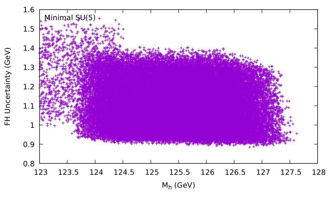
Figure 5.3: Left: The lightest Higgs mass, $M_{h}$, as a function of $M$ for the Minimal $N=1$ $SU(5)$ model. The $B$-physics constraints allow (mostly) higher scale points (with green colour). Right: The lightest Higgs mass theoretical uncertainty [79].

Large parts of the predicted particle spectrum are in agreement with the $B$-physics observables and the lightest Higgs boson mass measurement and its theoretical uncertainty. In order to test the models discovery potential, three benchmarks are selected, marking the points with the lightest SUSY particle (LSP) above $1200$ GeV (MINI-1), $1500$ GeV (MINI-2) and $2200$ GeV (MINI-3), respectively. The mass of the LSP can go as high as $\sim 3800\,\,\mathrm{GeV}$, but the cross sections calculated below will then be negligible and we restrict ourselves here to the low-mass region. The values presented in Tab. 5.1 were used as input to get the full supersymmetric spectrum from SPheno 4.0.4 [80, 81]. $M_{i}$ are the gaugino masses and the rest are squared soft sfermion masses which are diagonal ($\mathbf{m^{2}}=\rm diag(m_{1}^{2},m_{2}^{2},m_{3}^{2})$), and soft trilinear couplings (also diagonal $\mathbf{A_{i}}=\mathbb{1}_{3\times 3}A_{i}$).

	$M_{1}$	$M_{2}$	$M_{3}$	$|\mu|$	$b\leavevmode\nobreak\ \leavevmode\nobreak\ \leavevmode\nobreak\$	$A_{u}$	$A_{d}$	$A_{e}$	$\tan{\beta}$	$m_{Q_{1,2}}^{2}$
MINI-1	1227	2228	5310	4236	$401^{2}$	4325	4772	1732	50.3	$6171^{2}$
MINI-2	1507	2721	6376	5091	$496^{2}$	5245	5586	2005	52.0	$7445^{2}$
MINI-3	2249	4019	9138	7367	$1246^{2}$	7571	8317	3271	50.3	$10762^{2}$
	$m_{Q_{3}}^{2}$	$m_{L_{1,2}}^{2}$	$m_{L_{3}}^{2}$	$m_{\overline{u}_{1,2}}^{2}$	$m_{\overline{u}_{3}}^{2}$	$m_{\overline{d}_{1,2}}^{2}$	$m_{\overline{d}_{3}}^{2}$	$m_{\overline{e}_{1,2}}^{2}$	$m_{\overline{e}_{3}}^{2}$
MINI-1	$4548^{2}$	$3714^{2}$	$2767^{2}$	$5974^{2}$	$4181^{2}$	$5478^{2}$	$4177^{2}$	$4160^{2}$	$2491^{2}$
MINI-2	$5469^{2}$	$4521^{2}$	$3358^{2}$	$7206^{2}$	$5039^{2}$	$5478^{2}$	$4994^{2}$	$5070^{2}$	$3019^{2}$
MINI-3	$7890^{2}$	$6639^{2}$	$4934^{2}$	$10412^{2}$	$7233^{2}$	$9495^{2}$	$7211^{2}$	$7459^{2}$	$4464^{2}$

Table 5.1: Minimal $N=1$ $SU(5)$ predictions that are used as input to SPheno. Mass parameters are in $\,\,\mathrm{GeV}$ and rounded to $1\,\,\mathrm{GeV}$.

The resulting masses of all the particles that will be relevant for our analysis can be found in Tab. 5.2. The three first values are the heavy Higgs masses. The gluino mass is $M_{\tilde{g}}$, the neutralinos and the charginos are denoted as $M_{\tilde{\chi}_{i}^{0}}$ and $M_{\tilde{\chi}_{i}^{\pm}}$, while the slepton and sneutrino masses for all three generations are given as $M_{\tilde{e}_{1,2,3}},\leavevmode\nobreak\ M_{\tilde{\nu}_{1,2,3}}$. Similarly, the squarks are denoted as $M_{\tilde{d}_{1,2}}$ and $M_{\tilde{u}_{1,2}}$ for the first two generations. The third generation masses are given by $M_{\tilde{t}_{1,2}}$ for stops and $M_{\tilde{b}_{1,2}}$ for sbottoms.

	$M_{H}$	$M_{A}$	$M_{H^{\pm}}$	$M_{\tilde{g}}$	$M_{\tilde{\chi}^{0}_{1}}$	$M_{\tilde{\chi}^{0}_{2}}$	$M_{\tilde{\chi}^{0}_{3}}$	$M_{\tilde{\chi}^{0}_{4}}$	$M_{\tilde{\chi}_{1}^{\pm}}$	$M_{\tilde{\chi}_{2}^{\pm}}$
MINI-1	2.660	2.660	2.637	5.596	1.221	2.316	4.224	4.225	2.316	4.225
MINI-2	3.329	3.329	3.300	6.717	1.500	2.827	5.076	5.077	2.827	5.078
MINI-3	8.656	8.656	8.631	9.618	2.239	4.176	7.357	7.358	4.176	7.359
	$M_{\tilde{e}_{1,2}}$	$M_{\tilde{\nu}_{1,2}}$	$M_{\tilde{\tau}}$	$M_{\tilde{\nu}_{\tau}}$	$M_{\tilde{d}_{1,2}}$	$M_{\tilde{u}_{1,2}}$	$M_{\tilde{b}_{1}}$	$M_{\tilde{b}_{2}}$	$M_{\tilde{t}_{1}}$	$M_{\tilde{t}_{2}}$
MINI-1	3.729	3.728	2.445	2.766	5.617	6.100	4.332	4.698	4.312	4.704
MINI-2	4.539	4.538	2.968	3.356	6.759	7.354	5.180	5.647	5.197	5.652
MINI-3	6.666	6.665	4.408	4.935	9.722	10.616	7.471	8.148	7.477	8.151

Table 5.2: Masses of Higgs bosons and some of the SUSY particles for each benchmark of the Minimal $N=1$ $SU(5)$ (in TeV).

Table 5.3 shows the expected production cross section for selected channels at the 100 TeV future FCC-hh collider. We do not show any cross sections for $\sqrt{s}=14$ TeV, since the prospects for discovery of MINI scenarios at the HL-LHC are very dim. SUSY particles are too heavy to be produced with cross sections greater that 0.01 fb. Concerning the heavy Higgs bosons, the main search channels will be $H/A\to\tau^{+}\tau^{-}$. Our heavy Higgs-boson mass scale shows values $\;\raisebox{-3.00003pt}{$\stackrel{{\scriptstyle\displaystyle>}}{{\sim}}$}\;2500$ GeV with $\tan\beta\sim 50$. The corresponding reach of the HL-LHC has been estimated in [193]. In comparison with our benchmark points we conclude that they will not be accessible at the HL-LHC.

The situation changes for the FCC-hh. Theory analyses [194, 195] have shown that for large $\tan\beta$ heavy Higgs-boson mass scales up to $\sim 8$ TeV may be accessible, both for neutral as well as for charged Higgs bosons. The relevant decay channels are $H/A\to\tau^{+}\tau^{-}$ and $H^{\pm}\to\tau\nu_{\tau},tb$. This places our three benchmark points well within the covered region (MINI-1 and MINI-2) or at the border of the parameter space that can be probed (MINI-3).

The energy of 100 TeV is big enough to produce SUSY particles in pairs. However, the cross sections remain relatively small. Only for the MINI-1 scenario the squark pair and squark-gluino (summed over all squarks) production cross sections can reach tens of fb. For MINI-2 and MINI-3 scenarios the cross sections are significantly smaller. In these scenarios squarks decay preferentially into a quark+LSP (with $\rm BR\sim 0.95$), gluino into $\tilde{t}\bar{t}$ and $\tilde{b}\bar{b}$ +$h.c$ with $\rm BR\sim 0.33$ each.

The SUSY discovery reach at the FCC-hh with $3\,\mbox{ab}^{-1}$ was evaluated in [196] for a certain set of simplified models. In the following we will compare these simplified model limits with our benchmark points to get an idea, which part of the spectrum can be covered at the FCC-hh. A more detailed evaluation with the future limits implemented into proper recasting tools would be necessary to obtain a firmer statement. However, such a detailed analysis goes beyond the scope of our paper and we restrict ourselves to the simpler direct comparison of the simplified model limits with our benchmark predictions.

scenarios	MINI-1	MINI-2	MINI-3	scenarios	MINI-1	MINI-2	MINI-3
$\sqrt{s}$	100 TeV	100 TeV	100 TeV	$\sqrt{s}$	100 TeV	100 TeV	100 TeV
$\tilde{\chi}^{0}_{1}\tilde{\chi}^{0}_{1}$	0.04	0.02		$\tilde{u}_{i}\tilde{\chi}^{-}_{1},\tilde{d}_{i}\tilde{\chi}^{+}_{1}+h.c.$	1.00	0.35	0.03
$\tilde{\chi}^{0}_{1}\tilde{\chi}^{0}_{3}$	0.02	0.01		$\tilde{u}_{i}\tilde{\chi}^{-}_{2},\tilde{d}_{i}\tilde{\chi}^{+}_{2}+h.c.$	0.07	0.02
$\tilde{\chi}^{0}_{2}\tilde{\chi}^{0}_{2}$	0.06	0.02		$\tilde{q}_{i}\tilde{\chi}^{0}_{1},\tilde{q}_{i}^{*}\tilde{\chi}^{0}_{1}$	0.38	0.14	0.02
$\tilde{\chi}^{0}_{2}\tilde{\chi}^{0}_{3}$	0.03	0.01		$\tilde{q}_{i}\tilde{\chi}^{0}_{2},\tilde{q}_{i}^{*}\tilde{\chi}^{0}_{2}$	0.51	0.17	0.02
$\tilde{\chi}^{0}_{2}\tilde{\chi}^{0}_{4}$	0.02	0.01		$\tilde{\nu}_{i}\tilde{e}_{j}^{*},\tilde{\nu}_{i}^{*}\tilde{e}_{j}$	0.06	0.02
$\tilde{\chi}^{0}_{3}\tilde{\chi}^{0}_{4}$	0.05	0.02		$Hb\bar{b}$	84.04	30.10	0.17
$\tilde{\chi}^{0}_{2}\tilde{\chi}_{1}^{+}$	2.20	0.98	0.18	$Ab\bar{b}$	84.79	29.79	0.18
$\tilde{\chi}^{0}_{3}\tilde{\chi}_{2}^{+}$	0.10	0.04	0.01	$H^{+}b\bar{t}+H^{-}t\bar{b}$	33.24	12.76	0.1
$\tilde{\chi}^{0}_{4}\tilde{\chi}_{2}^{+}$	0.10	0.04	0.01	$H^{-}b\bar{b}$	0.04	0.02
$\tilde{g}\tilde{g}$	7.76	2.02	0.11	$Ht\bar{t}$	0.03	0.01
$\tilde{g}\tilde{\chi}^{0}_{1}$	0.28	0.11	0.01	$At\bar{t}$	0.02	0.01
$\tilde{g}\tilde{\chi}^{0}_{2}$	0.34	0.12	0.01	$Htb$	0.01
$\tilde{g}\tilde{\chi}_{1}^{+}$	0.70	0.27	0.03	$HA$	0.03	0.01
$\tilde{q}_{i}\tilde{q}_{j},\tilde{q}_{i}\tilde{q}_{j}^{*}$	21.15	7.44	0.74	$HH^{+}$	0.06	0.02
$\tilde{\chi}_{1}^{+}\tilde{\chi}_{1}^{-}$	1.19	0.54	0.09	$H^{+}W^{-}$	6.50	2.96	0.03
$\tilde{\chi}_{1}^{+}\tilde{\chi}_{2}^{-}$	0.05	0.02		$HW^{+}$	0.02	0.01
$\tilde{\chi}_{2}^{+}\tilde{\chi}_{1}^{-}$	0.05	0.02		$H^{+}H^{-}$	0.04	0.01
$\tilde{\chi}_{2}^{+}\tilde{\chi}_{2}^{-}$	0.06	0.02		$AH^{+}$	0.06	0.02
$\tilde{e}_{i}\tilde{e}_{j}^{*}$	0.16	0.08	0.01	$AW^{+}$	0.02	0.01
$\tilde{q}_{i}\tilde{g},\tilde{q}_{i}^{*}\tilde{g}$	30.57	9.33	0.66	$HZ$	1.38	0.58	0.01
$\tilde{\nu}_{i}\tilde{\nu}_{j}^{*}$	0.04	0.02		$AZ$	1.20	0.52	0.01

Table 5.3: Expected production cross sections (in fb) for SUSY particles in the MINI scenarios. There are no channels with cross sections exceeding 0.01 fb at $\sqrt{s}=14$ TeV.

Concerning the scalar tops, the mass predictions of MINI-1 and MINI-2 are well within the anticipated reach of the FCC-hh, while MINI-3 predicts a too heavy stop mass. On the other hand, even for MINI-1 and MINI-2 no $5\sigma$ discovery can be expected. The situation looks more favorable for the first and second generation squarks. All the predicted masses can be excluded at the FCC-hh, whereas a $5\sigma$ discovery will be difficult, but potentially possible (see Fig. 19 in [196]). Even more favorable appear the prospects for gluino searches at the FCC-hh. All three benchmark points may lead to a $5\sigma$ discovery (see Fig. 13 in [196]). On the other hand, chances for chargino/neutralino searches are slim at the FCC-hh. The Next-to LSP (NLSP) can only be accessed for $m_{\tilde{\chi}^{0}_{1}}\;\raisebox{-3.00003pt}{$\stackrel{{\scriptstyle\displaystyle<}}{{\sim}}$}\;1$ TeV (see Fig. 21 in [196]), where all our benchmark points have $m_{\tilde{\chi}^{0}_{1}}>1$ TeV. Taking into account that our three benchmark points represent only the lower part of the possible mass spectrum (with LSP masses of up to $\sim 1.5\,\,\mathrm{TeV}$ higher), we conclude that even at the FCC-hh large parts of the possible SUSY spectrum will remain elusive.

No point fulfills the strict bound of Eq. (5.9), since the relic abundance turns out to be too high, as it can be seen in Fig. 5.4. The model features a Bino-like neutralino, which proves too heavy to give an acceptable relic density. It is $\lesssim 5\%$ Higgsino-like and the Wino contribution is negligible. Thus, our model needs a mechanism that can reduce the CDM abundance in the early universe. This issue could be related to the problem of neutrino masses. These masses cannot be generated naturally in this particular model, although a non-zero value for neutrino masses has been established [180]. However, the model could be, in principle, extended by introducing bilinear R-parity violating terms and introduce neutrino masses [197, 198]. R-parity violation [199] would remove the CDM bound of Eq. (5.9) completely. Other mechanisms, not involving R-parity violation, that could be invoked if the amount of CDM appears to be too large, concern the cosmology of the early universe. For example, “thermal inflation” [200] or “late time entropy injection” [201] can bring the CDM density into agreement with WMAP measurements.

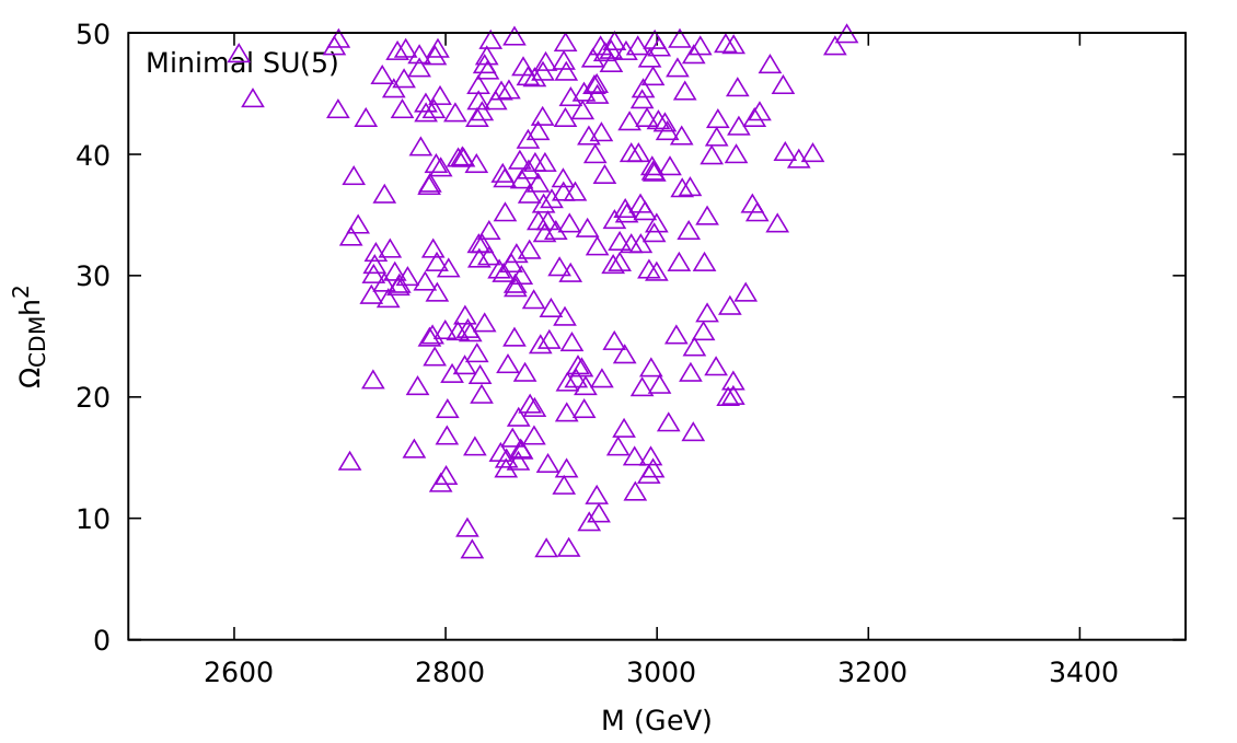
Figure 5.4: The plot shows the CDM relic density of the Minimal $N=1$ $SU(5)$ model for points with Higgs mass within its calculated uncertainty. Only the points with the lowest relic density are displayed.

5.4 The Finite $N=1$ $SU(5)$

This section contains the full particle spectrum predicted in the Finite $N=1$ SUSY $SU(5)$ model, as discussed in Sect. 4.2. The gauge symmetry breaks spontaneously below the GUT scale, so conditions set by finiteness do not restrict the  renormalization properties at low energies. We are left with boundary conditions on the gauge and Yukawa couplings (4.7), the $h=-MC$ relation and the soft scalar-mass sum rule at $M_{\rm GUT}$. Again, the uncertainty for the boundary conditions of the Yukawa couplings is at $7\%$, which again is included in the spread of the points.

In Fig. 5.5, $m_{b}(M_{Z})$ and $m_{t}$ are shown as functions of the unified gaugino mass $M$, where the green points satisfy the B-physics constraints with the same colour coding as in Fig. 5.2. Here we omitted the additional theoretical uncertainty of $\sim 6\,\,\mathrm{MeV}$. The only phenomenologically viable option is to consider $\mu<0$, as is shown in earlier work [202, 203, 204]. The experimental values are indicated by the horizontal lines with the uncertainties at the $2\,\sigma$ and $3\,\sigma$ level. The value of the bottom mass is lower than in past analyses, sending the allowed energy scale higher. Also the top-quark mass turns out slightly lower than in previous analyses.

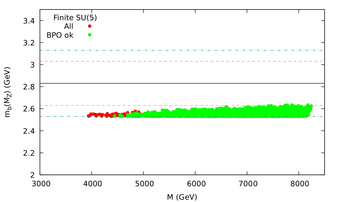
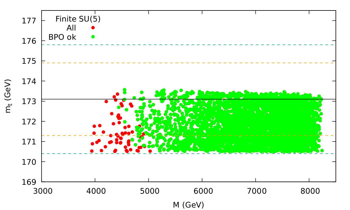
Figure 5.5: $m_{b}(M_{Z})$ (left) and $m_{t}$ (right) as a function of $M$ for the Finite $N=1$ $SU(5)$, with the colour coding as in Fig. 5.2.

The light Higgs boson mass is given in Fig. 5.6 (left) as a function of the unified gaugino mass. Like in the previous section, these predictions are subject to a theory uncertainty [79] that is given in Fig. 5.6 (right). This point-by-point uncertainty (calculated with FeynHiggs) drops significantly from the flat estimate of 2 and 3 GeV of past analyses to the much improved $0.65-0.70\,\,\mathrm{GeV}$. The $B$-physics constraints (green points) and the smaller Higgs uncertainty drive the energy scale above $\sim 4.5\,\,\mathrm{TeV}$. Older analyses, including in particular less refined evaluations of the light Higgs mass, are given in Refs. [202, 203, 204]. It should be noted that, w.r.t. previous analyses the top-quark mass turns out to be slightly lower. Consequently, higher scalar top masses have to be reached in order to yield the Higgs-boson mass around its central value of Eq. (5.3), resulting in a correspondingly heavier spectrum. Compared to our previous analyses [205, 202, 206, 203, 204, 207], the improved evaluation of $M_{h}$ and its uncertainty, together with a lower prediction of the top-quark mass prefers a heavier Higgs and SUSY spectrum. In particular, very heavy coloured SUSY particles are favoured (nearly independent of the $M_{h}$ uncertainty), in agreement with the non-observation of those particles at the LHC [208].

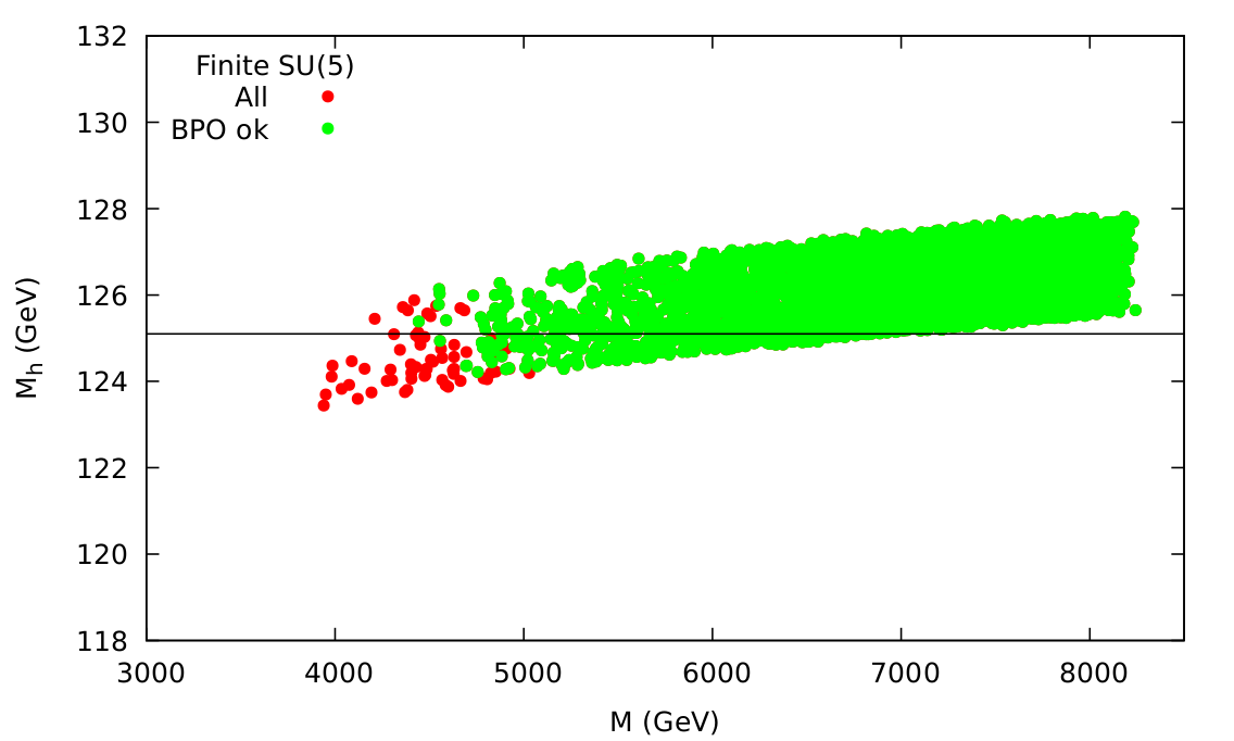
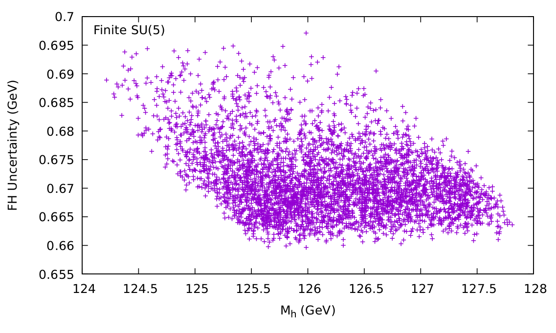
Figure 5.6: Left: $M_{h}$ as a function of $M$. Green points comply with $B$-physics constraints. Right: The lightest Higgs mass theoretical uncertainty calculated with FeynHiggs 2.16.0 [79].

For the purpose of testing the discovery potential we choose three benchmarks, each featuring the LSP above $2100$ GeV, $2400$ GeV and $2900$ GeV respectively. Again, they are chosen from the low-mass region. Although the LSP can be as heavy as $\sim 4000\,\,\mathrm{GeV}$, but in such cases the production cross sections even at the FCC-hh would be too small. The input and output of SPheno 4.0.4 [80, 81] can be found in Tab. 5.4 and Tab. 5.5 (with the notation as in Sect. 4.1).

	$M_{1}$	$M_{2}$	$M_{3}$	$|\mu|$	$b\leavevmode\nobreak\ \leavevmode\nobreak\ \leavevmode\nobreak\$	$A_{u}$	$A_{d}$	$A_{e}$	$\tan{\beta}$	$m_{Q_{1,2}}^{2}$
FUTSU5-1	2124	3815	8804	4825	$854^{2}$	7282	7710	2961	49.9	$8112^{2}$
FUTSU5-2	2501	4473	10198	5508	$1048^{2}$	8493	9023	3536	50.1	$9387^{2}$
FUTSU5-3	3000	5340	11996	6673	$2361^{2}$	10086	10562	4243	49.9	$11030^{2}$
	$m_{Q_{3}}^{2}$	$m_{L_{1,2}}^{2}$	$m_{L_{3}}^{2}$	$m_{\overline{u}_{1,2}}^{2}$	$m_{\overline{u}_{3}}^{2}$	$m_{\overline{d}_{1,2}}^{2}$	$m_{\overline{d}_{3}}^{2}$	$m_{\overline{e}_{1,2}}^{2}$	$m_{\overline{e}_{3}}^{2}$
FUTSU5-1	$6634^{2}$	$3869^{2}$	$3120^{2}$	$7684^{2}$	$5053^{2}$	$7635^{2}$	$4177^{2}$	$3084^{2}$	$2241^{2}$
FUTSU5-2	$7669^{2}$	$4521^{2}$	$3747^{2}$	$8887^{2}$	$6865^{2}$	$8826^{2}$	$6893^{2}$	$3602^{2}$	$2551^{2}$
FUTSU5-3	$9116^{2}$	$5355^{2}$	$3745^{2}$	$10419^{2}$	$8170^{2}$	$10362^{2}$	$7708^{2}$	$4329^{2}$	$3403^{2}$

Table 5.4: Finite $N=1$ $SU(5)$ predictions that are used as input to SPheno. Mass parameters are in $\,\,\mathrm{GeV}$ and rounded to $1\,\,\mathrm{GeV}$.

The expected production cross sections for various final states are listed in Table 5.6. At 14 TeV HL-LHC none of the Finite $N=1$ $SU(5)$ scenarios listed in Table 5.4 has a SUSY production cross section above 0.01 fb, and thus will (likely) remain unobservable. All superpartners are too heavy to be produced in pairs. Also the heavy Higgs bosons are far outside the reach of the HL-LHC [193].

	$M_{H}$	$M_{A}$	$M_{H^{\pm}}$	$M_{\tilde{g}}$	$M_{\tilde{\chi}^{0}_{1}}$	$M_{\tilde{\chi}^{0}_{2}}$	$M_{\tilde{\chi}^{0}_{3}}$	$M_{\tilde{\chi}^{0}_{4}}$	$M_{\tilde{\chi}_{1}^{\pm}}$	$M_{\tilde{\chi}_{2}^{\pm}}$
FUTSU5-1	5.688	5.688	5.688	8.966	2.103	3.917	4.829	4.832	3.917	4.833
FUTSU5-2	7.039	7.039	7.086	10.380	2.476	4.592	5.515	5.518	4.592	5.519
FUTSU5-3	16.382	16.382	16.401	12.210	2.972	5.484	6.688	6.691	5.484	6.691
	$M_{\tilde{e}_{1,2}}$	$M_{\tilde{\nu}_{1,2}}$	$M_{\tilde{\tau}}$	$M_{\tilde{\nu}_{\tau}}$	$M_{\tilde{d}_{1,2}}$	$M_{\tilde{u}_{1,2}}$	$M_{\tilde{b}_{1}}$	$M_{\tilde{b}_{2}}$	$M_{\tilde{t}_{1}}$	$M_{\tilde{t}_{2}}$
FUTSU5-1	3.102	3.907	2.205	3.137	7.839	7.888	6.102	6.817	6.099	6.821
FUTSU5-2	3.623	4.566	2.517	3.768	9.059	9.119	7.113	7.877	7.032	7.881
FUTSU5-3	4.334	5.418	3.426	3.834	10.635	10.699	8.000	9.387	8.401	9.390

Table 5.5: Masses for each benchmark of the Finite $N=1$ $SU(5)$ (in TeV).

At the FCC-hh the discovery prospects for the heavy Higgs-boson spectrum is significantly better. With $\tan\beta\sim 50$ the first two benchmark points, FUTSU5-1 and FUTSU5-2, are well within the reach of the FCC-hh. The third point, FUTSU5-3, however, with $M_{A}\sim 16$ TeV will be far outside the reach of the FCC-hh. Prospects for detecting production of squark pairs and squark-gluino pairs are also very dim since their production cross section is also at the level of a few fb. This is as a result of a heavy spectrum in this class of models (see [196] with the same Figures as discussed in Sec. 4.1).

scenarios	FUTSU5-1	FUTSU5-2	FUTSU5-3	scenarios	FUTSU5-1	FUTSU5-2	FUTSU5-3
$\sqrt{s}$	100 TeV	100 TeV	100 TeV	$\sqrt{s}$	100 TeV	100 TeV	100 TeV
$\tilde{\chi}^{0}_{2}\tilde{\chi}^{0}_{3}$	0.01	0.01		$\tilde{\nu}_{i}\tilde{\nu}_{j}^{*}$	0.02	0.01	0.01
$\tilde{\chi}^{0}_{3}\tilde{\chi}^{0}_{4}$	0.03	0.01		$\tilde{u}_{i}\tilde{\chi}^{-}_{1},\tilde{d}_{i}\tilde{\chi}^{+}_{1}+h.c.$	0.15	0.06	0.02
$\tilde{\chi}^{0}_{2}\tilde{\chi}_{1}^{+}$	0.17	0.08	0.03	$\tilde{q}_{i}\tilde{\chi}^{0}_{1},\tilde{q}_{i}^{*}\tilde{\chi}^{0}_{1}$	0.08	0.03	0.01
$\tilde{\chi}^{0}_{3}\tilde{\chi}_{2}^{+}$	0.05	0.03	0.01	$\tilde{q}_{i}\tilde{\chi}^{0}_{2},\tilde{q}_{i}^{*}\tilde{\chi}^{0}_{2}$	0.08	0.03	0.01
$\tilde{\chi}^{0}_{4}\tilde{\chi}_{2}^{+}$	0.05	0.03	0.01	$\tilde{\nu}_{i}\tilde{e}_{j}^{*},\tilde{\nu}_{i}^{*}\tilde{e}_{j}$	0.09	0.04	0.01
$\tilde{g}\tilde{g}$	0.20	0.05	0.01	$Hb\bar{b}$	2.76	0.85
$\tilde{g}\tilde{\chi}^{0}_{1}$	0.03	0.01		$Ab\bar{b}$	2.73	0.84
$\tilde{g}\tilde{\chi}^{0}_{2}$	0.03	0.01		$H^{+}b\bar{t}+h.c.$	1.32	0.42
$\tilde{g}\tilde{\chi}_{1}^{+}$	0.07	0.03	0.01	$H^{+}W^{-}$	0.38	0.12
$\tilde{q}_{i}\tilde{q}_{j},\tilde{q}_{i}\tilde{q}_{j}^{*}$	3.70	1.51	0.53	$HZ$	0.09	0.03
$\tilde{\chi}_{1}^{+}\tilde{\chi}_{1}^{-}$	0.10	0.05	0.02	$AZ$	0.09	0.03
$\tilde{\chi}_{2}^{+}\tilde{\chi}_{2}^{-}$	0.03	0.02	0.01
$\tilde{e}_{i}\tilde{e}_{j}^{*}$	0.23	0.13	0.05
$\tilde{q}_{i}\tilde{g},\tilde{q}_{i}^{*}\tilde{g}$	2.26	0.75	0.20

Table 5.6: Expected production cross sections (in fb) for SUSY particles in the FUTSU5 scenarios.

Concerning the stops, the lighter one might be accessible in FUTSU5-1. For the squarks of the first two generations the prospects of testing the model are somewhat better. All three benchmark models could possibly be excluded at the $2\sigma$ level, but no discovery at the $5\sigma$ can be expected. The same holds for the gluino. Charginos and neutralinos will remain unobservable due to the heavy LSP. As in the previous section, since only the lower part of the possible mass spectrum has been considered (with LSP masses higher by up to $\sim 1\,\,\mathrm{TeV}$), we have to conclude that again large parts of the possible mass spectra will not be observable at the FCC-hh.

Concerning DM, the model exhibits a high relic abundance for CDM, as it can be seen in Fig. 5.7. Again, the neutralino is strongly Bino-like, not allowing for a relic density within experimental limits. The CDM alternatives proposed for the Minimal $SU(5)$ model can also be applied here. It should be noted that the bilinear R-parity violating terms proposed in the previous section preserve finiteness, as well.

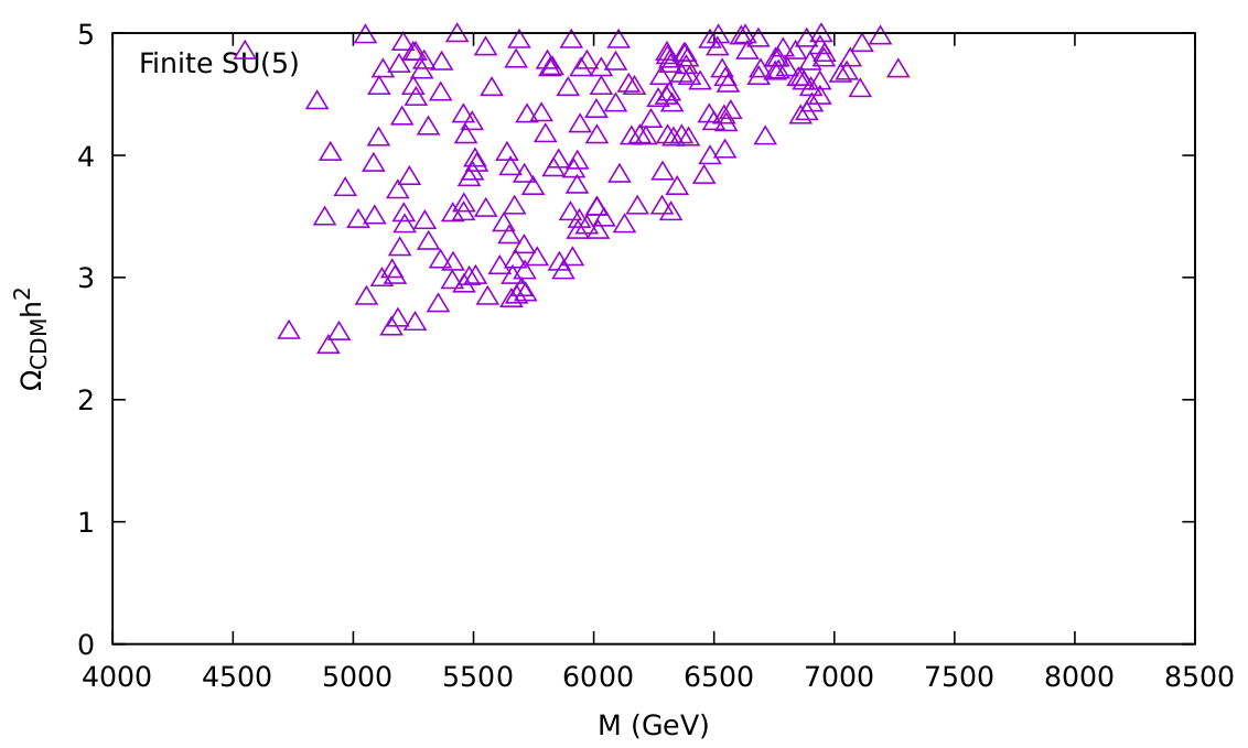
Figure 5.7: The plot shows the CDM relic density of the Finite $N=1$ $SU(5)$ model for points with Higgs mass within its calculated uncertainty. Only the points with the lowest relic density are displayed.

5.5 The Two-Loop Finite $N=1$ $SU(3)\otimes SU(3)\otimes SU(3)$

The analysis of the two-loop finite $N=1$ SUSY $SU(3)\otimes SU(3)\otimes SU(3)$ model, as described in the Sect. 4.3, is the focus of this section. Again, below $M_{\rm GUT}$ we get the MSSM. We further assume a unique SUSY breaking scale $M_{\rm SUSY}$ and below that scale the effective theory is just the SM. The boundary condition uncertainty is at $5\%$ for the Yukawa couplings and at $1\%$ for the strong gauge coupling and the soft parameters.

We take into account two new thresholds for the masses of the new exotic particles at $\sim 10^{13}\,\,\mathrm{GeV}$ and $\sim 10^{14}\,\,\mathrm{GeV}$. This results in a wider phenomenologically viable parameter space [209]. Specifically, one of the down-like exotic particles decouples at $10^{14}\,\,\mathrm{GeV}$  while the rest decouple at $10^{13}\,\,\mathrm{GeV}$.

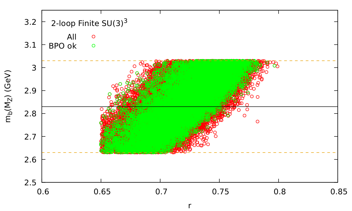
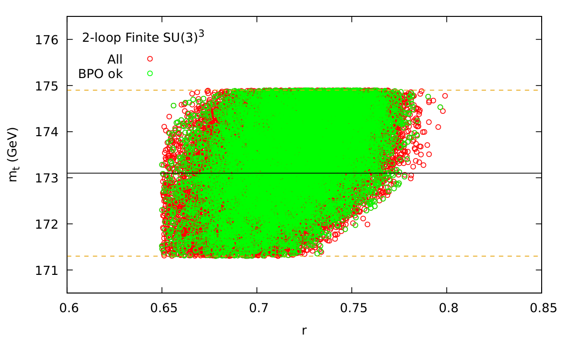
Figure 5.8: Bottom and top quark  masses for the Finite $N=1$ $SU(3)\otimes SU(3)\otimes SU(3)$ model, with $\mu<0$, as functions of $r$. The colour coding is as in Fig. 5.2.

We compare our predictions with the experimental value of $m_{t}^{\rm exp}$, while in the case of the bottom quark we take again the value evaluated at $M_{Z}$, see Eq. (5.1). We single out the $\mu<0$ case as the most promising model. With the inclusion of thresholds for the decoupling of the exotic particles, the parameter space allowed predicts a top quark mass in agreement with experimental bounds (see Eq. (5.2)), which is an important improvement from past versions of the model [27, 210, 211, 212]. Looking for the values of the parameter $r$ (see Sect. 4.3) which comply with the experimental limits (see Sect. 5.1) for $m_{b}(M_{Z})$ and $m_{t}$, we find, as shown in Fig. 5.8, that both masses are in the experimental range for the same value of $r$ between $0.65$ and $0.80$. It is important to note that the two masses are simultaneously within two sigmas of the experimental bounds.

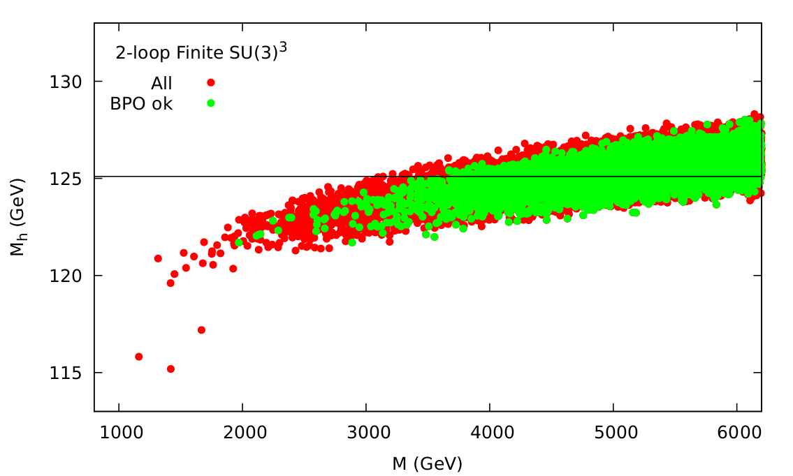
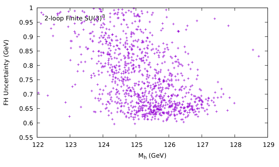
Figure 5.9: Left: $M_{h}$ as a function of $M$ for the Finite $N=1$ $SU(3)\otimes SU(3)\otimes SU(3)$. Right: The Higgs mass theoretical uncertainty [79].

In Fig. 5.9 (left) the light Higgs boson mass is shown as a function of the unified gaugino mass, while with the point-by-point calculated theoretical uncertainty drops below 1 GeV [79] (Fig. 5.9 (right)). As in the previous models examined, the $B$-physics constraints (green points in Fig. 5.9 (left) satisfy them) and the new, more restrictive Higgs mass uncertainty exclude most of the low range of $M$, pushing the particle spectrum to higher values.

	$M_{1}$	$M_{2}$	$M_{3}$	$|\mu|$	$b\leavevmode\nobreak\ \leavevmode\nobreak\ \leavevmode\nobreak\$	$A_{u}$	$A_{d}$	$A_{e}$	$\tan{\beta}$	$m_{Q_{1,2}}^{2}$
FSU33-1	1522	2758	6369	6138	$1002^{2}$	4520	4413	1645	46.2	$5574^{2}$
FSU33-2	2070	3722	8330	7129	$1083^{2}$	5841	5734	2357	45.5	$7255^{2}$
FSU33-3	2500	4484	10016	6790	$972^{2}$	7205	7110	2674	49.7	$8709$
	$m_{Q_{3}}^{2}$	$m_{L_{1,2}}^{2}$	$m_{L_{3}}^{2}$	$m_{\overline{u}_{1,2}}^{2}$	$m_{\overline{u}_{3}}^{2}$	$m_{\overline{d}_{1,2}}^{2}$	$m_{\overline{d}_{3}}^{2}$	$m_{\overline{e}_{1,2}}^{2}$	$m_{\overline{e}_{3}}^{2}$
FSU33-1	$4705^{2}$	$2382^{2}$	$3754^{2}$	$5234^{2}$	$5548^{2}$	$5197^{2}$	$7043^{2}$	$1558^{2}$	$3095^{2}$
FSU33-2	$7255^{2}$	$3136^{2}$	$4131^{2}$	$6749^{2}$	$7225^{2}$	$6745^{2}$	$8523^{2}$	$2238^{2}$	$3342^{2}$
FSU33-3	$9074^{2}$	$3831^{2}$	$5483^{2}$	$8152^{2}$	$7207^{2}$	$2558^{2}$	$8600^{2}$	$2507^{2}$	$4000^{2}$

Table 5.7: Finite $N=1$ $SU(3)^{3}$ predictions that are used as input to SPheno. Mass parameters are in $\,\,\mathrm{GeV}$ and rounded to $1\,\,\mathrm{GeV}$.

Again, we choose three benchmarks, each featuring the LSP above $1500$ GeV, $2000$ GeV and $2400$ GeV respectively (but the LSP can go as high as $\sim 4100\,\,\mathrm{GeV}$, again with too small cross sections). The input and output of SPheno 4.0.4 [80, 81] can be found in Tab. 5.7 and Tab. 5.8 respectively (with the notation as in Sect. 4.1).

It should be noted that in this model the scale of the heavy Higgs bosons does not vary monotonously with $m_{\tilde{\chi}^{0}_{1}}$, as in the previously considered models. This can be understood as follows.  The Higgs bosons masses are determined by a combination of the sum rule at the unification scale, and the requirement of successful electroweak symmetry breaking at the low scale. Like in the finite scenario of the previous section, there are no direct relations between the soft scalar masses and the unified gaugino mass, but they are related through the corresponding sum rule and thus vary correlatedly, a fact that makes the dependence on the boundary values more restrictive. Furthermore (and even more importantly), the fact that we took into account the two thresholds at $\sim 10^{13}\,\,\mathrm{GeV}$ and $\sim 10^{14}\,\,\mathrm{GeV}$ (as mentioned above), allows the new particles, mainly the Higgsinos of the two other families (that were considered decoupled at the unification scale in previous analyses) and the down-like exotic quarks (in a lower degree), to affect the running of the (soft) RGEs in a non-negligible way. Thus, since at low energies the heavy Higgs masses depend mainly on the values of $m^{2}_{H_{u}}$, $m^{2}_{H_{d}}$, $|\mu|$ and $\tan\beta$, they are substantially less connected to $m_{\tilde{\chi}^{0}_{1}}$ than in the other models, leading to a different exclusion potential, as  will be discussed in the following.

	$M_{H}$	$M_{A}$	$M_{H^{\pm}}$	$M_{\tilde{g}}$	$M_{\tilde{\chi}^{0}_{1}}$	$M_{\tilde{\chi}^{0}_{2}}$	$M_{\tilde{\chi}^{0}_{3}}$	$M_{\tilde{\chi}^{0}_{4}}$	$M_{\tilde{\chi}_{1}^{\pm}}$	$M_{\tilde{\chi}_{2}^{\pm}}$
FSU33-1	7.029	7.029	7.028	6.526	1.506	2.840	6.108	6.109	2.839	6.109
FSU33-2	6.484	6.484	6.431	8.561	2.041	3.817	7.092	7.093	3.817	7.093
FSU33-3	6.539	6.539	6.590	10.159	2.473	4.598	6.780	6.781	4.598	6.781
	$M_{\tilde{e}_{1,2}}$	$M_{\tilde{\nu}_{1,2}}$	$M_{\tilde{\tau}}$	$M_{\tilde{\nu}_{\tau}}$	$M_{\tilde{d}_{1,2}}$	$M_{\tilde{u}_{1,2}}$	$M_{\tilde{b}_{1}}$	$M_{\tilde{b}_{2}}$	$M_{\tilde{t}_{1}}$	$M_{\tilde{t}_{2}}$
FSU33-1	2.416	2.415	1.578	2.414	5.375	5.411	4.913	5.375	4.912	5.411
FSU33-2	3.188	3.187	2.269	3.186	7.026	7.029	6.006	7.026	6.005	7.029
FSU33-3	3.883	3.882	2.540	3.882	8.334	8.397	7.227	8.334	7.214	7.409

Table 5.8: Masses for each benchmark of the Finite $N=1$ $SU(3)^{3}$ (in TeV).

Scenarios of Finite $SU(3)^{3}$ are beyond the reach of the HL-LHC. Not only superpartners are too heavy, but also heavy Higgs bosons with a mass scale of $\sim 7$ TeV cannot be detected at the HL-LHC. At 100 TeV collider (see Tab. 5.9), on the other hand, all three benchmark points are well within the reach of the $H/A\to\tau^{+}\tau^{-}$ as well as the $H^{\pm}\to\tau\nu_{\tau},tb$ searches [194, 195], despite the slightly smaller values of $\tan\beta\sim 45$. This is particularly because of the different dependence of the heavy Higgs-boson mass scale on $m_{\tilde{\chi}^{0}_{1}}$, as discussed above. However, we have checked that $M_{A}$ can go up to to $\sim 11\,\,\mathrm{TeV}$, and thus the heaviest part of the possible spectrum would escape the heavy Higgs-boson searches at the FCC-hh.

Interesting are also the prospects for production of squark pairs and squark-gluino, which can reach $\sim 20$ fb for the FSU33-1 case, going down to a few fb for FSU33-2 and FSU33-3 scenarios. The lightest squarks decay almost exclusively  to the third generation quark and chargino/neutralino, while gluino enjoys many possible decay channels to quark-squark pairs each one with branching fraction of the order of a percent, with the biggest one $\sim 20\%$ to $t\tilde{t}_{1}+h.c.$.

We briefly discuss the SUSY discovery potential at the FCC-hh, referring again to [196] with the same Figures as discussed in Sec. 4.1. Stops in FSU33-1 and FSU33-2 can be tested at the FCC-hh, while the masses turn out to be too heavy in FSU33-3. The situation is better for scalar quarks, where all three scenarios can be tested, but will not allow for a $5\sigma$ discovery. Even more favorable are the prospects for gluino. Possibly all three scenarios can be tested at the $5\sigma$ level. As in the previous scenario, the charginos and neutralinos will not be accessible, due to the too heavy LSP. Keeping in mind that only the lower part of possible mass spectrum  is represented by the three benchmarks (with the LSP up to $\sim 1.5\,\,\mathrm{TeV}$ heavier), we conclude that as before large parts of the parameter space will not be testable at the FCC-hh. The only partial exception here is the Higgs-boson sector, where only the the part with the highest possible Higgs-boson mass spectra would escape the FCC-hh searches.

scenarios	FSU33-1	FSU33-2	FSU33-3	scenarios	FSU33-1	FSU33-2	FSU33-3
$\sqrt{s}$	100 TeV	100 TeV	100 TeV	$\sqrt{s}$	100 TeV	100 TeV	100 TeV
$\tilde{\chi}^{0}_{1}\tilde{\chi}^{0}_{1}$	0.04	0.01	0.01	$\tilde{q}_{i}\tilde{g},\tilde{q}_{i}^{*}\tilde{g}$	22.12	3.71	1.05
$\tilde{\chi}^{0}_{2}\tilde{\chi}^{0}_{2}$	0.04	0.01		$\tilde{\nu}_{i}\tilde{\nu}_{j}^{*}$	0.10	0.03	0.01
$\tilde{\chi}^{0}_{2}\tilde{\chi}_{1}^{+}$	0.58	0.16	0.07	$\tilde{u}_{i}\tilde{\chi}^{-}_{1},\tilde{d}_{i}\tilde{\chi}^{+}_{1}+h.c.$	1.22	0.25	0.08
$\tilde{\chi}^{0}_{3}\tilde{\chi}_{2}^{+}$	0.02	0.01	0.01	$\tilde{q}_{i}\tilde{\chi}^{0}_{1},\tilde{q}_{i}^{*}\tilde{\chi}^{0}_{1}$	0.55	0.13	0.05
$\tilde{\chi}^{0}_{4}\tilde{\chi}_{2}^{+}$	0.02	0.01	0.01	$\tilde{q}_{i}\tilde{\chi}^{0}_{2},\tilde{q}_{i}^{*}\tilde{\chi}^{0}_{2}$	0.60	0.13	0.04
$\tilde{g}\tilde{g}$	2.61	0.30	0.07	$\tilde{\nu}_{i}\tilde{e}_{j}^{*},\tilde{\nu}_{i}^{*}\tilde{e}_{j}$	0.36	0.12	0.04
$\tilde{g}\tilde{\chi}^{0}_{1}$	0.20	0.05	0.02	$Hb\bar{b}$	0.71	1.23	1.19
$\tilde{g}\tilde{\chi}^{0}_{2}$	0.20	0.04	0.01	$Ab\bar{b}$	0.72	1.23	1.18
$\tilde{g}\tilde{\chi}_{1}^{+}$	0.42	0.09	0.03	$H^{+}b\bar{t}+h.c.$	0.37	0.75	0.58
$\tilde{q}_{i}\tilde{q}_{j},\tilde{q}_{i}\tilde{q}_{j}^{*}$	25.09	6.09	2.25	$H^{+}W^{-}$	0.10	0.25	0.19
$\tilde{\chi}_{1}^{+}\tilde{\chi}_{1}^{-}$	0.37	0.10	0.04	$HZ$	0.02	0.04	0.04
$\tilde{e}_{i}\tilde{e}_{j}^{*}$	0.39	0.12	0.06	$AZ$	0.02	0.04	0.04

Table 5.9: Expected production cross sections (in fb) for SUSY particles in the FSU33 scenarios.

The only observable that fails to comply with the experimental bounds is the CDM relic density (see Eq. (5.9)), as evident in Fig. 5.10. The lightest neutralino is the LSP and considered as a CDM candidate, but its relic density does not go below $0.15$, since it is strongly Bino-like and would require a lower scale of the particle spectrum. It should be noted that if the B-physics constraints allowed for a unified gaugino mass $\sim 0.5\,\,\mathrm{TeV}$ lower, then agreement with the CDM bounds as well could be achieved.

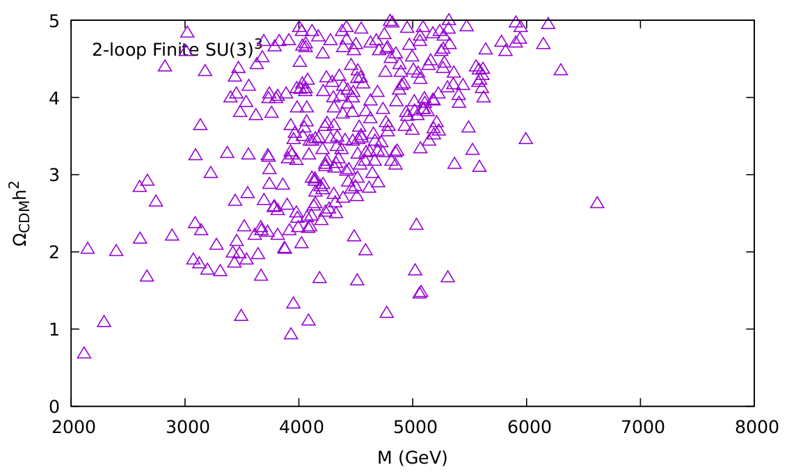
Figure 5.10: The plot shows the CDM relic density of the two-loop Finite $N=1$ $SU(3)\otimes SU(3)\otimes SU(3)$ model model for points with Higgs mass within its calculated uncertainty.

5.6 The Reduced MSSM

The last analysis is the one for the reduced version of the MSSM. The relations among reduced parameters in terms of the fundamental ones derived in Sect. 4.4 have an RGI part and a part that originates from the corrections, and thus scale dependent. In the present analysis we choose the unification scale to apply the corrections to all these RGI relations. As noted earlier, the Hisano-Shiftman relation sets a hierarchy among the gaugino masses, rendering Wino the lightest of them. As such, we have a Wino-like lightest neutralino.

In the dimensionless sector of the theory, since $Y_{\tau}$ is not reduced in favour of the fundamental parameter $\alpha_{3}$, the tau lepton mass is an input parameter and, consequently, $\rho_{\tau}$ is an independent parameter, too. At low energies we fix $\rho_{\tau}$ and $\tan\beta$ using the mass of the tau lepton $m_{\tau}(M_{Z})=1.7462$ GeV. Then, we determine the top and bottom masses using the value found for $\tan\beta$ together with $G_{t,b}$, as obtained from the REs and their corrections.

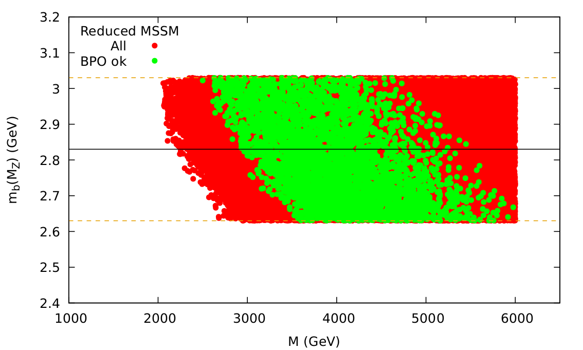
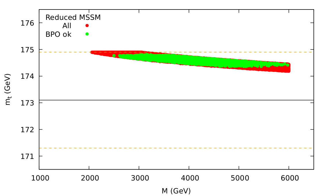
Figure 5.11: The left (right) plot shows the bottom (top) quark mass for the Reduced MSSM, with the colour coding as in Fig. 5.2.

Correspondingly, concerning the dimensionful sector, $h_{\tau}$ cannot be expressed in terms of the unified gaugino mass scale, leaving $\rho_{h_{\tau}}$ a free parameter. $\mu$ is a free parameter as well, as it cannot be reduced in favour of $M_{3}$ as discussed above. On the other hand, $m_{3}^{2}$ could be reduced, but here we choose to leave it free. However, $\mu$ and $m_{3}^{2}$ are restricted from the requirement of EWSB, and only $\mu$ is taken as an independent parameter. Finally, the other parameter in the Higgs-boson sector, the ${\cal CP}$-odd Higgs-boson mass $M_{A}$ is evaluated from $\mu$, as well as from $m_{H_{u}}^{2}$ and $m_{H_{d}}^{2}$, which are obtained from the REs. In total, we vary the parameters $\rho_{\tau}$, $\rho_{h_{\tau}}$, $M$ and $\mu$.

As it has been already mentioned, the variation of $\rho_{\tau}$ gives the running bottom quark mass at the $Z$ boson mass scale and the top pole mass, where points not within $2\sigma$ of the experimental data are neglected, as it is shown in Fig. 5.11. The experimental values (see Sect. 5.1) are denoted by the horizontal lines with the uncertainties at the $2\,\sigma$ level. The green dots satisfy the flavour constraints. One can see that the scan yields many parameter points that are in very good agreement with the experimental data and give restrictions in the allowed range of $M$ (the common gaugino mass at the unification scale).

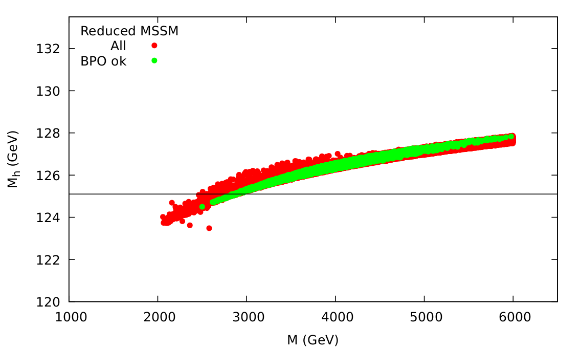
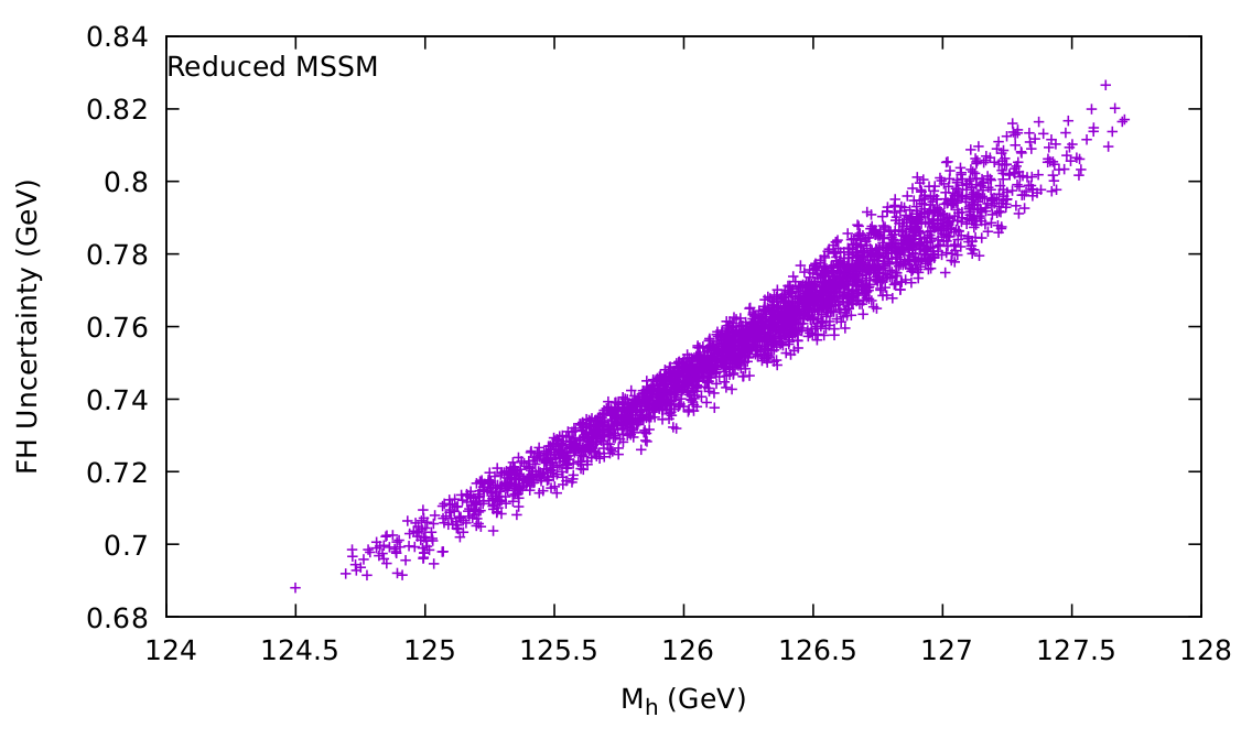
Figure 5.12: Left: The lightest Higgs boson mass, $M_{h}$ in the Reduced MSSM. The green points is the full model prediction. Right: the lightest Higgs mass theoretical uncertainty [79].

The prediction for $M_{h}$ is shown in Fig. 5.12 (left). Once again, one should keep in mind that the theory uncertainty given in Fig. 5.12 (right) has dropped below 1 GeV [79]. The Higgs mass predicted by the model is in the range measured at the LHC, favoring this time relatively small values of $M$. This in turn sets a limit on the low-energy SUSY masses, rendering the Reduced MSSM highly predictive and testable.

The $M_{h}$ limits set a limit on the low-energy supersymmetric masses, which we briefly discuss. The three selected benchmarks correspond to $\overline{\mathrm{DR}}$  pseudoscalar Higgs boson masses above $1900$ GeV, $1950$ GeV and $2000$ GeV respectively. The input of SPheno 4.0.4 [80, 81] can be found in Tab. 5.10 (notation as in Sect. 4.1).

	$M_{1}$	$M_{2}$	$M_{3}$	$|\mu|$	$b\leavevmode\nobreak\ \leavevmode\nobreak\ \leavevmode\nobreak\$	$A_{u}$	$A_{d}$	$A_{e}$	$\tan{\beta}$	$m_{Q_{1,2}}^{2}$
RMSSM-1	3711	1014	7109	4897	$284^{2}$	5274	5750	20	44.9	$5985^{2}$
RMSSM-2	3792	1035	7249	4983	$294^{2}$	5381	5871	557	44.6	$6103^{2}$
RMSSM-3	3829	1045	7313	5012	$298^{2}$	5427	5942	420	45.3	$6161^{2}$
	$m_{Q_{3}}^{2}$	$m_{L_{1,2}}^{2}$	$m_{L_{3}}^{2}$	$m_{\overline{u}_{1,2}}^{2}$	$m_{\overline{u}_{3}}^{2}$	$m_{\overline{d}_{1,2}}^{2}$	$m_{\overline{d}_{3}}^{2}$	$m_{\overline{e}_{1,2}}^{2}$	$m_{\overline{e}_{3}}^{2}$
RMSSM-1	$5545^{2}$	$2106^{2}$	$2069^{2}$	$6277^{2}$	$5386^{2}$	$5989^{2}$	$5114^{2}$	$3051^{2}$	$4491^{2}$
RMSSM-2	$5656^{2}$	$2122^{2}$	$2290^{2}$	$6385^{2}$	$5476^{2}$	$6110^{2}$	$5219^{2}$	$3153^{2}$	$4181^{2}$
RMSSM-3	$5708^{2}$	$2106^{2}$	$2279^{2}$	$6427^{2}$	$5506^{2}$	$6172^{2}$	$5269^{2}$	$3229^{2}$	$3504^{2}$

Table 5.10: Reduced MSSM predictions that are used as input to SPheno Mass parameters are in $\,\,\mathrm{GeV}$ and rounded to $1\,\,\mathrm{GeV}$.

Concerning the DM predictions, it should be noted that the Hisano-Shiftman relation imposes a Wino-like LSP, which unfortunately lowers the CDM relic density below the boundaries of Eq. (5.9). This can be seen in Fig. 5.13. This could render the model viable if Eq. (5.9) is applied only as an upper limit and additional sources of CDM are allowed. This is in contrast to the other three models discussed previously.

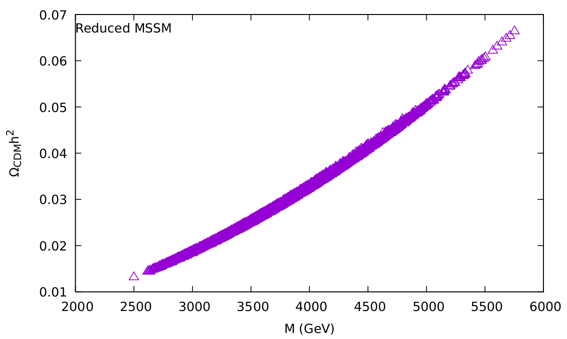
Figure 5.13: The plot shows the CDM relic density of the Reduced MSSM for points with Higgs mass within its calculated uncertainty. All points are below the experimental limits.

Table 5.11 shows the resulting masses of Higgs bosons and some of the lightest SUSY particles. In particular, we find $M_{A}\;\raisebox{-3.00003pt}{$\stackrel{{\scriptstyle\displaystyle<}}{{\sim}}$}\;1.5\,\,\mathrm{TeV}$ (for large values of $\tan\beta$ as in the other models), values substantially lower than in the previously considered models. This can be understood as follows.

	$M_{H}$	$M_{A}$	$M_{H^{\pm}}$	$M_{\tilde{g}}$	$M_{\tilde{\chi}^{0}_{1}}$	$M_{\tilde{\chi}^{0}_{2}}$	$M_{\tilde{\chi}^{0}_{3}}$	$M_{\tilde{\chi}^{0}_{4}}$	$M_{\tilde{\chi}_{1}^{\pm}}$	$M_{\tilde{\chi}_{2}^{\pm}}$
RMSSM-1	1.393	1.393	1.387	7.253	1.075	3.662	4.889	4.891	1.075	4.890
RMSSM-2	1.417	1.417	1.414	7.394	1.098	3.741	4.975	4.976	1.098	4.976
RMSSM-3	1.491	1.491	1.492	7.459	1.109	3.776	5.003	5.004	1.108	5.004
	$M_{\tilde{e}_{1,2}}$	$M_{\tilde{\nu}_{1,2}}$	$M_{\tilde{\tau}}$	$M_{\tilde{\nu}_{\tau}}$	$M_{\tilde{d}_{1,2}}$	$M_{\tilde{u}_{1,2}}$	$M_{\tilde{b}_{1}}$	$M_{\tilde{b}_{2}}$	$M_{\tilde{t}_{1}}$	$M_{\tilde{t}_{2}}$
RMSSM-1	2.124	2.123	2.078	2.079	6.189	6.202	5.307	5.715	5.509	5.731
RMSSM-2	2.297	2.139	2.140	2.139	6.314	6.324	5.414	5.828	5.602	5.842
RMSSM-3	2.280	2.123	2.125	2.123	6.376	6.382	5.465	5.881	5.635	5.894

Table 5.11: Masses for each benchmark of the Reduced MSSM (in TeV).

In this model, we have direct relations between the soft scalar masses and the unified gaugino mass, which receive corrections from the two gauge couplings $g_{1}$ and $g_{2}$ and the Yukawa coupling of the $\tau$ lepton. As mentioned above, in the absence of these corrections the relations obey the soft scalar mass sum rule. However, unlike all the previous models, these corrections make the sum rule only approximate. Thus, these unique boundary conditions result in very low values for the masses of the heavy Higgs bosons (even compared to the minimal $SU(5)$ case presented above, which also exhibits direct relations which however obey the sum rule). A relatively light spectrum is also favored by the prediction for the light CP-even Higgs boson mass, which turns out to be relatively high in this model and does not allow us to consider heavier spectra. Thus, in this model, contrary to the models analyzed before, because of the large $\tan\beta\sim 45$ found here, the physical mass of the pseudoscalar Higgs boson, $M_{A}$, is excluded by the searches $H/A\rightarrow\tau\tau$ at ATLAS with 139/fb [171] for all three benchmarks. One could try considering a heavier spectrum, in which we would have $M_{A}\gtrsim 1900\,\,\mathrm{GeV}$, but in that case the light Higgs mass would be well above its acceptable region. Particularly, it would be above 128 GeV, a value that is clearly excluded, especially given the improved (much smaller) uncertainty calculated by the new FeynHiggs code). Thus, the current version of this model has been ruled out experimentally. Consequently, we do not show any SUSY or Higgs production cross sections.

Part II Trinification from Coset Space Dimensional Reduction

Chapter 6 The Coset Space Dimensional Reduction

Consider a unified theory that is built on a spacetime in higher than four dimensions. Such a higher-dimensional theory can lead to a four-dimensional theory through the dimensional reduction procedure. The very first approach of such reduction of a unified higher-dimensional theory to a four-dimensional one was made by Kaluza and Klein [213, 214]. The main idea was to begin by considering a pure five-dimensional gravitational theory and perform a dimensional reduction which would lead to a four-dimensional theory, specifically a theory of electromagnetism coupled to gravity. Moreover, an appealing aspect of the whole dimensional reduction scheme is that the extension of the spacetime naturally leads to non-Abelian group structures [215, 216, 217] (for reviews see [218, 219, 220]).

The initial spacetime in high dimensions, $M^{D}$, can be considered as $M^{D}=M^{4}\times B$, where $B$ is a Riemannian manifold which is compact and its isometries are described by a group $S$. If a dimensional reduction is applied on the higher-dimensional theory, the resulting theory would be a four-dimensional one describing gravity and a Yang-Mills theory. The non-Abelian gauge group of the Yang-Mills part of the four-dimensional theory would include the isometry group of $B$, that is $S$, accompanied by scalar fields. Besides the main and most important aspect of the above scheme, namely the unification of the gravitational interaction with others that are described by gauge theories in a geometric way, it is also very welcome that the above scheme sheds light on the fact that some interactions admit a description of a gauge theory.

On the other hand, there are also some unwelcome features that emerge after performing the above dimensional reduction. First, expressing the higher-dimensional space $M^{D}$ as a product does not allow for a classical ground state. Although the Ricci tensor of a space like the one considered, $B$, is non-vanishing, the field equations of the initial, pure $D$-dimensional gravitational theory yield that the Ricci tensor is equal to zero. Thus, it is deduced that the extra dimensions cannot be interpreted in a physical way. Additionally, another serious drawback in the attempt to result in realistic four-dimensional models is that performing a dimensional reduction of a higher-dimensional theory in which fermions are accommodated does not allow to end up with chiral fermions in the resulting four-dimensional theory [221]. Nevertheless, it is possible to overcome the above problems by choosing an appropriate spectrum of particles in the higher-dimensional theory, specifically involving Yang-Mills fields [222, 41].

Putting aside gravitational phenomena in the low-energy regime implies the consideration of the initial higher-dimensional theory to be purely Yang-Mills (Y-M). Performing a dimensional reduction could lead to a (probably unified) four-dimensional Yang-Mills theory accompanied by a Higgs sector. A naive way way to perform such a reduction on a Y-M theory defined on $M^{D}=M^{4}\times B$ is to impose the condition that every particle of the spectrum depends only on the $M^{4}$ spacetime coordinates. Therefore, considering every particle independent of the extra coordinates implies that the Lagrangian density would also not depend on them. A less crude approach is to consider that the part of the space related to the extra dimensions is described by a coset space $B=S/R$. The elegance of this approach lies in the fact that one does not have to impose any independence of the fields on the extra dimensions. More specifically, the fields are allowed to depend on the coordinates of the extra dimensions in such a way that an application of an S-transformation would transform the Lagrangian by some quantity that would be cancelled by a simple gauge transformation. In other words, the Lagrangian ends up to be independent of the extra (coset) coordinates because of its gauge invariance, which is a built-in property, and not because of an arbitrary demand. This is the most fundamental argument that renders the Coset Space Dimensional Reduction (CSDR) a very appealing scheme for the treatment of higher-dimensional theories and the construction of promising four-dimensional theories [36, 37, 38].

6.1 Coset Space Geometry

Before we proceed to the description of the CSDR scheme, it is useful to recall some basic information about the geometry of coset spaces. This section includes the prerequisite geometrical aspects of coset spaces needed in order to understand the CSDR scheme. For an extended (and more complete) discussion of the geometry of coset spaces see [37, 223].

In the CSDR scheme one starts by considering a Yang-Mills-Dirac (YMD) action with a gauge group $G$. The action is defined on a spacetime of $D$ dimensions, $M^{D}$ and its metric is $g^{MN}$. The spacetime $M^{D}$ gets compactified to the spacetime $M^{4}\times S/R$, with $S/R$ a coset space. The metric of the compactified space has the following block diagonal form:

$$g^{MN}=\left[\begin{array}[]{cc}\eta^{\mu\nu}&0\\ 0&-g^{ab}\end{array}\right],$$ (6.1)

where $\eta^{\mu\nu}=\text{diag}(1,-1,-1,-1)$ and $g^{ab}$ is the metric of the coset space. The above compactification of the initial spacetime points to further exploration of the geometry of coset spaces $S/R$, where $S$ is a compact Lie group and $R$ is compact Lie subgroup of $S$.

It is useful to divide the set of the generators of the group $S$, $Q_{A}$, into two subsets, one including the generators of $R$, $Q_{i}$ $(i=1,\ldots,\text{dim}R)$ and another including the generators of $S/R$, $Q_{a}$, where $a=\text{dim}R+1\ldots,\text{dim}S$, with $\text{dim}(S/R)=\text{dim}S-\text{dim}R=d$. Therefore, their commutation relations can be written in the following form:

$$\left[Q_{i},Q_{j}\right] = f_{ij}^{\ \ k}Q_{k}\ ,$$

$$\left[Q_{i},Q_{a}\right] = f_{ia}^{\ \ b}Q_{b}\ ,$$

$$\left[Q_{a},Q_{b}\right] = f_{ab}^{\ \ i}Q_{i}+f_{ab}^{\ \ c}Q_{c}\ .$$ (6.2)

The second commutation relation demonstrates the fact that the coset space $S/R$ is reductive (since $R$ is compact) and, in general, non-symmetric.

Now, let us denote the coordinates of the compactified space $M^{4}\times S/R$ as $z^{M}=(x^{m},y^{\alpha})$, where $\alpha$ is a curved index of the coset space and $y$ is a parametrization of an element of $S$, which is actually a coset representative, $L(y)$. Latin indices $a,b,\ldots$ will denote the coordinates of the tangent space. The vielbein and the $R$-connection are defined by the Maurer-Cartan form which takes its values in the Lie algebra of $S$ :

$$L^{-1}(y)dL(y)=e^{A}_{\alpha}Q_{A}dy^{\alpha}\leavevmode\nobreak\ .$$ (6.3)

At the origin it holds that $y=0$, $e^{\leavevmode\nobreak\ a}_{\alpha}=\delta^{\leavevmode\nobreak\ a}_{\alpha}$ and $e^{\leavevmode\nobreak\ i}_{\alpha}=0$. In general, a connection form $\theta^{a}_{\ b}$ on $S/R$ consists of both curvature and torsion. In the case that the torsion vanishes, the calculation of the torsionless part $\omega^{a}_{\ b}$ takes place by setting the torsion form, $T^{a}$, to zero:

$$T^{a}=de^{a}+\omega^{a}_{\ b}\wedge e^{b}=0\ ,$$ (6.4)

while using the Maurer-Cartan equation

$$de^{a}=\frac{1}{2}f^{a}_{\ bc}e^{b}\wedge e^{c}+f^{a}_{\ bi}e^{b}\wedge e^{i}\ ,$$ (6.5)

one obtains the following expression for the connection

$$\omega^{a}_{\ b}=-f^{a}_{\ ib}e^{i}-\frac{1}{2}f^{a}_{\ bc}e^{c}-\frac{1}{2}K^{a}_{\ bc}e^{c}\ ,$$ (6.6)

where $K^{a}_{\ bc}$ is symmetric under the exchange of the lower indices $b,c$, thus $K^{a}_{\ bc}e^{c}\wedge e^{b}=0$. The expression of the $K^{a}_{\ bc}$ can be obtained by taking into consideration that $\omega^{a}_{\ b}$ is antisymmetric, that is $\omega^{a}_{\ b}g^{cb}=-\omega^{b}_{\ c}g^{ca}$:

$$K_{\ \ bc}^{a}=g^{ad}(g_{be}f_{dc}^{\ \ e}+g_{ce}f_{db}^{\ \ e})\ .$$ (6.7)

In turn, replacing the above expression for $K^{a}_{\ bc}$ in the expression for $\omega^{a}_{\ b}$, (6.6), one obtains the following form of the connection:

$$\omega^{a}_{\ b}=-f^{a}_{\ ib}e^{i}-D_{\ bc}^{a}e^{c},$$ (6.8)

where

$$D_{\ bc}^{a}=\frac{1}{2}g^{ad}[f_{db}^{\ \ e}g_{ec}+f_{cb}^{\ \ e}g_{de}-f_{cd}^{\ \ e}g_{be}]\ .$$ (6.9)

According to [37], the $D$’s can be related to the structure constants by a rescaling:

$$D^{a}_{\ bc}=(\lambda^{a}\lambda^{b}/\lambda^{c})f^{a}_{\ bc}\ ,$$

where the $\lambda$’s depend only on the radii of the coset. It should be noted that, in general, the rescaling factors affect the antisymmetry properties of the structure constants. Also, in the case that the radii are equal, it holds:

$$D^{a}_{\ bc}=\frac{1}{2}f^{a}_{\ bc}\ .$$ (6.10)

Moreover, the connection form $\omega^{a}_{\ b}$ is $S$-invariant, meaning that a parallel transport commutes with the $S$ action [223]. Consequently, the most general expression of an $S$-invariant connection on $S/R$ is:

$$\omega^{a}_{\ b}=f_{\ \ ib}^{a}e^{i}+J_{\ \ cb}^{a}e^{c}\ ,$$ (6.11)

with $J$ being a tensor that is $R$-invariant, namely:

$$\delta J_{cb}^{\ \ a}=-f_{ic}^{\ \ d}J_{db}^{\ \ a}+f_{id}^{\ \ a}J_{cb}^{\ \ d}-f_{ib}^{\ \ d}J_{cd}^{\ \ a}=0.$$

It can be easily shown -using the Jacobi identity- that the $D$ tensor, given in Eq. (6.9), satisfies the above condition.

Then, for the case of non-vanishing torsion the expression is:

$$T^{a}=de^{a}+\Omega^{a}_{\ b}\wedge e^{b}\ ,$$ (6.12)

where the connection $\Omega^{a}_{\ b}$ is expressed as a decomposition of two parts:

$$\Omega^{a}_{\ b}=\omega^{a}_{\ b}+\tau^{a}_{\ b}\ .$$

The first is the connection of the torsionless case mentioned above and the second is given by:

$$\tau^{a}_{\ b}=-\frac{1}{2}\Sigma^{a}_{\ bc}e^{c},$$ (6.13)

where $\Sigma^{a}_{\ \ bc}$ is the contorsion, expressed as

$$\Sigma^{a}_{\ bc}=T^{a}_{\ \ bc}+T_{bc}^{\ \ a}-T_{cb}^{\ \ a}$$ (6.14)

in terms of the torsion components $T^{a}_{\ bc}$. Therefore, putting all the expressions of the connections together, the general connection form $\theta^{a}_{\ b}$ is written as:

$$\Omega^{a}_{\ b}=-f^{a}_{\ ib}e^{i}-\left(D^{a}_{\ bc}+\frac{1}{2}\Sigma^{a}_{\ bc}\right)e^{c}=-f^{a}_{\ ib}e^{i}-G^{a}_{\ bc}e^{c}\ .$$ (6.15)

In the case of equal radii, it is possible to express $T^{a}_{\ bc}$ as $T^{a}_{\ bc}=\eta f^{a}_{\ bc}$, where $\eta$ is a parameter [45, 46, 224, 225, 226]. A natural generalization of the expression of $T^{a}_{\ bc}$ in the case of unequal radii would be $T^{a}_{\ bc}=2\tau D^{a}_{\ bc}$, where $\tau$ is another parameter. The latter was obtained after taking into consideration and generalizing the expression of $D^{a}_{\ bc}$ for equal radii, Eq. (6.10). However, generalizing the case of equal radii to the relation $T^{a}_{\ bc}=2\tau D^{a}_{\ bc}$ for different radii turns out to be insufficient, as the $D^{a}_{\ bc}$ fail to have the appropriate symmetry properties. In order to ameliorate this drawback, the $\Sigma$ is defined as a combination of $D^{a}_{\ bc}$ in such a way that it is rendered completely antisymmetric and, at the same time, $S$-invariant:

$$\Sigma_{abc}\equiv 2\tau(D_{abc}+D_{bca}-D_{cba})\ .$$ (6.16)

Furthermore, the curvature two-form is given by the following expression [37], [225, 226]:

$$R^{a}_{\ b}=\left[-\frac{1}{2}f_{ib}^{\ a}f_{de}^{\leavevmode\nobreak\ \leavevmode\nobreak\ i}-\frac{1}{2}G_{cb}^{\leavevmode\nobreak\ \leavevmode\nobreak\ a}f_{de}^{\leavevmode\nobreak\ \leavevmode\nobreak\ c}+\frac{1}{2}(G_{dc}^{\leavevmode\nobreak\ \leavevmode\nobreak\ a}G_{eb}^{\leavevmode\nobreak\ \leavevmode\nobreak\ c}-G_{ec}^{\leavevmode\nobreak\ \leavevmode\nobreak\ a}G_{db}^{\leavevmode\nobreak\ \leavevmode\nobreak\ c})\right]e^{d}\wedge e^{e},$$ (6.17)

while the Ricci tensor, $R_{ab}=R^{d}_{\ adb}$, is obtained as:

$$R_{ab}=G_{ba}^{\leavevmode\nobreak\ \leavevmode\nobreak\ c}G_{dc}^{\leavevmode\nobreak\ \leavevmode\nobreak\ d}-G_{bc}^{\leavevmode\nobreak\ \leavevmode\nobreak\ d}G_{da}^{\leavevmode\nobreak\ \leavevmode\nobreak\ c}-G_{ca}^{\leavevmode\nobreak\ \leavevmode\nobreak\ d}f_{db}^{\leavevmode\nobreak\ \leavevmode\nobreak\ c}-f_{ia}^{\leavevmode\nobreak\ \leavevmode\nobreak\ d}f_{db}^{\leavevmode\nobreak\ \leavevmode\nobreak\ i}\ .$$ (6.18)

If we choose $\tau$ to vanish, then the corresponding connection is called Riemannian connection, $\Omega_{R\leavevmode\nobreak\ b}^{\leavevmode\nobreak\ a}$. Another special case worth mentioning is the canonical connection, which is obtained by adjusting both the radii and $\tau$ in such a way that the connection form is $\Omega_{C\leavevmode\nobreak\ \leavevmode\nobreak\ b}^{\leavevmode\nobreak\ a}=-f^{a}_{\leavevmode\nobreak\ bi}e^{i}$, that is an $R$-gauge field [45, 46]. Also, the adjustments of the parameters are such that satisfy $G_{abc}=0$. In the case of $SU(3)/(U(1)\times U(1))$ with metric $g_{ab}=\text{diag}(a,a,b,b,c,c)$, one needs to set $a=b=c$ and therefore consider that $\tau=-\frac{1}{3}$. Similar adjustments can cause the Ricci tensor [45, 46] to vanish, with the corresponding connection called Ricci flattening connection.

6.2 Main Features and Constraints of CSDR

We continue with the description of the main aspects of the CSDR that will be necessary in the next sections. Consider a Y-M theory in $D$ dimensions with gauge group by $G$. The action will be:

$$S =\int d^{4}xd^{d}y\sqrt{-g}\left[-\frac{1}{4}\text{Tr}(F_{MN}F_{K\Lambda})g^{MK}g^{N\Lambda}+\frac{i}{2}\bar{\psi}\Gamma^{M}D_{M}\psi\right]\,,$$ (6.19)

in which it is evident from the last term that fermionic fields have been introduced in the theory. the metric tensor of the $D$-dimensional spacetime is denoted $g_{MN}$  and $D_{M}$ is the covariant derivative expressed as

$$D_{M}=\partial_{M}-\theta_{M}-igA_{M}\,,\,\text{where}\,\,\,\theta_{M}=\frac{1}{2}\theta_{MN\Lambda}\Sigma^{N\Lambda}\,$$ (6.20)

is the spin connection of the spacetime. Furthermore, $\psi$ is a spinor representing the fermionic fields of the theory, which can be assigned into an arbitrary representation $F$ of $G$. Nevertheless, in a supersymmetric version of the theory, the fermions should be accommodated in the adjoint representation along with $A_{M}$, which is the gauge field related to $G$, forming a vector supermultiplet. Subsequently, $F_{MN}$ is the field strength tensor of $A_{M}$:

$$F_{MN}=\partial_{M}A_{N}-\partial_{N}A_{M}-ig[A_{M},A_{N}]\,.$$ (6.21)

Now, let the Killing vectors of $S/R$ be denoted as $\xi^{\alpha}_{A}$, where $A=1,\ldots,\text{dim}S$ and $\alpha=\text{dim}R+1,\ldots,\text{dim}S$. Let us also consider a gauge transformation, $W_{A}$, which is related to the Killing vector $\xi_{A}$. The condition that all kinds of fields (scalars $\phi$, spinors $\psi$ and vectors $A_{\alpha}$) that live on the coset space are symmetric is translated to the following constraints:

$$\delta_{A}\phi =\xi^{\leavevmode\nobreak\ \alpha}_{A}\partial_{\alpha}\phi=D(W_{A})\phi,$$ (6.22)

$$\delta_{A}A_{\alpha} =\xi^{\leavevmode\nobreak\ \beta}_{A}\partial_{\beta}A_{\alpha}+\partial_{\alpha}\xi^{\leavevmode\nobreak\ \beta}_{A}A_{\beta}=\partial_{\alpha}W_{A}-[W_{A},A_{\alpha}],$$ (6.23)

$$\delta_{A}\psi =\xi^{\leavevmode\nobreak\ \alpha}_{A}\partial_{\alpha}\psi-\frac{1}{2}G_{Abc}\Sigma^{bc}\psi=D(W_{A})\psi\,.$$ (6.24)

In the above, $D(W_{A})$ is the gauge transformation $W_{A}$ in the appropriate representation of the group according to the representation in which the various fields are assigned. The transformation $W_{A}$, no matter the representation, depends only on the coordinates of the coset space. The above equations of the constraints (6.22)-(6.24) are particularly important, since their solutions determine both the gauge group and the spectrum of the reduced, four-dimensional theory [36, 37]. Let us now work through the above constraints in some detail. First, the gauge field $A_{M}$ defined on the $D$-dimensional spacetime can be written explicitly in the split form $A_{M}=(A_{\mu},A_{\alpha})$, since $M^{D}=M^{4}\times S/R$. Under an $S$-transformation the four-dimensional part $A_{\mu}$ follows the transformation rule of a scalar field, which is obviously accommodated in the adjoint representation of the initial gauge group, $G$. The first constraint, (6.22), leads to two enlightening results:

• The gauge group of the four-dimensional theory is $H=C_{G}(R_{G})$, that is the centralizer of $R$ in $G$.

• The first part of the $(A_{\mu},A_{\alpha})$ is identified as the four-dimensional gauge field $A_{\mu}$ and does not depend on the coordinates of the coset space. Regarding the second component of the initial gauge field, $A_{\alpha}$, it is identified as a set of scalar fields in the four-dimensional theory, assuming the role of intertwining operators among the representations of $R$ in $G$ and in $S$. The latter is obtained by solving the second constraint, (6.23). The following decomposition of the initial gauge group $G$, along with the decomposition of $S$ under its subgroup $R$, give insight on the representation of the produced scalars in the four-dimensional theory:

  $$G\supset R_{G}\times H\,,\qquad\mathrm{adj}G=(\mathrm{adj}R,1)+(1,\mathrm{adj}H)+\sum(r_{i},h_{i})\,,$$ (6.25)

  $$S\supset R\,,\qquad\mathrm{adj}S=\mathrm{adj}R+\sum s_{i}\,.$$ (6.26)

  Given that the irreducible representations $r_{i}$ and $s_{i}$ of $R$ are identical, the representation $h_{i}$ of $H$ accounts for a scalar multiplet. Any scalars that are not included in $h_{i}$ vanish.

In turn, the third constraint in (6.24) is related to the spinorial part and its form and properties in the four-dimensional theory. The line of reasoning is similar to the one described above about the scalars [37, 40, 41, 227, 228, 229, 230]. By solving the third constraint it becomes apparent that the four-dimensional spinors, $\psi$, depend exclusively on the coordinates of the four-dimensional part. In addition, similarly to the scalar fields, $\psi$ relates the induced representations of $R$ between $SO(d)$ and $G$ as an intertwining operator. The representation of the four-dimensional gauge group$H$ in which fermions are assigned, denoted by $f_{i}$, is determined by the decomposition rule of the representation $F$ of $G$, that is the fermionic representation in the higher-dimensional theory, with respect to $R_{G}\times H$ and the spinorial representation of $SO(d)$ under $R$:

$$G\supset R_{G}\times H\,,\qquad F=\sum(r_{i},f_{i}),$$ (6.27)

$$SO(d)\supset R\,,\qquad\sigma_{d}=\sum\sigma_{j}\,.$$ (6.28)

Similarly to the scalar case examined above, the $r_{i}$ and $\sigma_{i}$ representations are effectively the same and for each pair of those an $f_{i}$ multiplet of four-dimensional spinors exists.

At this point a few comments on the nature of the fermions before and after the dimensional reduction are in order. If the fermions introduced in the theory in higher dimensions are considered to be Dirac-type, then the surviving ones in the four-dimensional theory will not be chiral, which is surely a most unwelcome feature. However, considering the higher-dimensional theory defined on an even-dimensional spacetime and imposing the Weyl condition, the fermions of the resulting four-dimensional theory will have the property of chirality. In particular, fermions that are assigned to the adjoint representation of a gauge group of a higher-dimensional theory defined on a spacetime of $D=2n+2$ dimensions and also obey the Weyl constraint, eventually result to two sets of chiral fermions in the four-dimensional theory with the quantum numbers being identical for the components of the two sets. If the condition imposed on the fermions of the higher-dimensional theory is extended to include the Majorana condition, then the doubling of the fermionic spectrum does not appear in the four-dimensional theory. Imposing both the Weyl and the Majorana conditions is possible when the dimensions of the initial theory are $D=4n+2$.

6.3 The action of the reduced four-dimensional theory

Let us now focus on the action of the four-dimensional theory, obtained after the dimensional reduction. First, consider that the higher-dimensional spacetime, $M^{D}$, is compactified as $M^{4}\times S/R$, where $S/R$ is a compact coset space. This kind of compactification induces the following modification on the form of the metric:

$$g^{MN}=\left(\begin{array}[]{cc}\eta^{\mu\nu}&0\\ 0&-g^{ab}\\ \end{array}\right)\,,$$ (6.29)

where the upper left block is the (mainly negative) four-dimensional Minkowski metric, while the lower right is the coset space metric tensor. Introducing the above metric in the Y-M action of the higher-dimensional theory given in Eq. (6.19) and taking into account the constraints (6.22)-(6.24), the reduced action of the four-dimensional theory is:

$$S=C\int d^{4}x\,\mathrm{tr}\left[-\frac{1}{8}F_{\mu\nu}F^{\mu\nu}-\frac{1}{4}(D_{\mu}\phi_{a})(D^{\mu}\phi^{a})\right]+V(\phi)+\frac{i}{2}\bar{\psi}\Gamma^{\mu}D_{\mu}\psi-\frac{i}{2}\bar{\psi}\Gamma^{a}D_{a}\psi\,,$$ (6.30)

in which:

• $C$ denotes the coset space volume

• $D_{\mu}=\partial_{\mu}-igA_{\mu}$ is the covariant derivative in four dimensions

• $D_{a}=\partial_{a}-\theta_{a}-ig\phi_{a}$ is the covariant derivative of the coset space, $\theta_{a}=\tfrac{1}{2}\theta_{abc}\Sigma^{bc}$ its connection and $\phi_{a}\equiv A_{a}$

• $V(\phi)$ is the four-dimensional scalar potential which can be explicitly written as:

  $$V(\phi)=-\frac{1}{8}g^{ac}g^{bd}\mathrm{Tr}(f^{\leavevmode\nobreak\ \leavevmode\nobreak\ C}_{ab}\phi_{C}-ig[\phi_{a},\phi_{b}])(f^{\leavevmode\nobreak\ \leavevmode\nobreak\ D}_{cd}\phi_{D}-ig[\phi_{c},\phi_{d}])\,,$$ (6.31)

  in which $A=1,...,\mathrm{dim}S$ and $f^{\leavevmode\nobreak\ \leavevmode\nobreak\ C}_{ab},f^{\leavevmode\nobreak\ \leavevmode\nobreak\ D}_{cd}$ are the structure constants of the algebra of $S$, which is the group of isometries of the coset.

Furthermore, the constraints (6.22) - (6.24) imply that for the scalars $\phi_{a}$ we have:

$$f^{\leavevmode\nobreak\ \leavevmode\nobreak\ D}_{ai}\phi_{D}-ig[\phi_{a},\phi_{i}]=0\,,$$ (6.32)

in which $\phi_{i}$ denote the generators of the subgroup $R_{G}$. The scalar fields that survive the dimensional reduction are identified as the Higgs sector of the four-dimensional theory. The vacuum of the theory is obtained by the minimization of the scalar potential $V(\phi)$ written down in (6.31) and eventually the corresponding gauge symmetry is obtained [231, 232, 233, 234, 235, 236, 237, 238]. In general, the procedure above is not straightforward and is indeed difficult to carry out. Nevertheless, in the very special case in which the isometry group of the coset space, $S$, has an isomorphic image (denoted as $S_{G}$) into $G$, then the four-dimensional gauge group $H$ breaks spontaneously in a subgroup of $H$, denoted $K$. The subgroup $K$ is obtained by the centralizer of the isomorphic image of $S$ in $G$ in the gauge group $G$ of the higher-dimensional theory [37, 231, 232, 233, 234, 235, 236, 237, 238]. The latter gets well-understood by the following scheme:

$$G\supset \,S_{G}\times K$$

$$\,\cup\quad\,\,\,\cap$$

$$G\supset \,R_{G}\times H\leavevmode\nobreak\ .$$ (6.33)

In case of a symmetric coset space (this means $f_{ab}^{\leavevmode\nobreak\ \leavevmode\nobreak\ c}=0$) the four-dimensional scalar potential always takes a form which allows the spontaneous symmetry breaking [37]. Although an unwelcome feature of the application of the above theorem is that the fermions of the four-dimensional theory appear to become supermassive [239] (similarly to the Kaluza-Klein case), there is an exceptional case in which fermions are prevented form acquiring superheavy masses.

Examining the fermionic part of the effective four-dimensional action, one has to focus on the last two terms of (6.30). The first term is identified as the fermionic kinetic term, while the second is related to Yukawa interactions. Since the fermions of the higher-dimensional theory are considered to be satisfying the Weyl and Majorana conditions, then they it is possible to assign them in a real representation of the initial gauge group. In particular, the last term (Yukawa term) of the Lagrangian of Eq. (6.30) can be expressed as:

$$L_{Y}=-\frac{i}{2}\bar{\psi}\Gamma^{a}(\partial_{a}-\frac{1}{2}f_{ibc}e_{\Gamma}^{i}e_{a}^{\Gamma}\Sigma^{bc}-\frac{1}{2}G_{abc}\Sigma^{bc}-\phi_{a})\psi=\frac{i}{2}\bar{\psi}\Gamma^{a}\nabla_{a}\psi+\bar{\psi}V\psi\,,$$ (6.34)

in which it is implied that

$$\nabla_{a} =-\partial_{a}+\frac{1}{2}f_{ibc}e_{\Gamma}^{i}e_{a}^{\Gamma}\Sigma^{bc}+\phi_{a},$$ (6.35)

$$V =\frac{i}{4}\Gamma^{a}G_{abc}\Sigma^{bc},$$ (6.36)

making use of the complete connection, that is the one including torsion [225, 226]. As mentioned in Sect. 6.2, the third constraint Eq. (6.24) implies that they do not depend on the coordinates of the coset space. Moreover, due to the invariance of the Lagrangian under $S$-transformations, it is equivalent to work with the Lagrangian in the special case in which $y=0$ and $e_{\Gamma}^{\leavevmode\nobreak\ i}$. Under these conditions, (6.35) is reduced to the following form:

$$\nabla_{a}=\phi_{a}$$ (6.37)

The fermionic fields are independent of the coset space coordinates (i.e. $\partial_{a}\psi=0$) since they are symmetric fields, satisfying the constraint equation Eq. (6.24). Furthermore, we can consider the Lagrangian at the point $y=0$ due to its invariance under $S$-tranformations and $e^{i}_{\Gamma}=0$ at that point. Therefore, Eq. (6.35) becomes just $\nabla_{a}=\phi_{a}$ and the term $\frac{i}{2}\bar{\psi}\Gamma^{a}\nabla_{a}\psi$ of Eq. (6.34) is identified exactly as a Yukawa term.

Further examining the last term of Eq. (6.34), one can easily show that $V$ and the six-dimensional operator of helicity are anticommutative [37], while, on the other hand, $V$ and $T_{i}=-\frac{1}{2}f_{ibc}\Sigma^{bc}$ are commutative quantities. Taking into consideration Schur’s lemma, it is deduced that the surviving terms of $V$ are those that are present in the decomposition of $4$ and $\bar{4}$ irreducible representations of $SO(6)$, namely the singlets. Due to their geometric origin the singlets will obtain masses in a very large scale, a fact that most likely leads to problematic phenomenology. In particular, the gauginos that appear in the four-dimensional theory after the application of the CSDR theme on a supersymmetric higher-dimensional theory will obtain masses at the order of the compactification scale. However, such an outcome is prevented by the inclusion of the torsion. This will be the case considered in the following construction.

6.4 CSDR and the Einstein-Yang-Mills Theory

Finally, consider the case of the Einstein-Yang-Mills (EYM) theory in $4+d$ dimensions, in which a cosmological constant is present. Such a system is described by the following Lagrangian density:

$${\cal L}=-\frac{1}{16\pi G}\sqrt{-g}R^{D}-\frac{1}{4e^{2}}\sqrt{-g}F^{a}_{\ MN}F^{aMN}-\sqrt{-g}\Lambda\,.$$ (6.38)

The corresponding equations of motion are obtained:

$$R_{MN}-\frac{1}{2}Rg_{MN} = -8\pi GT_{MN}\,,$$

$$D_{M}F^{MN} = 0\,.$$ (6.39)

in which the energy-momentum tensor, $T_{MN}$, of Eq. (6.4), has been identified as:

$$T_{MN}=\frac{1}{e^{2}}F^{a}_{\ MP}F^{a\ P}_{\ N}-g_{MN}\left(\frac{1}{e^{2}}F^{a}_{\leavevmode\nobreak\ PS}F^{aPS}+\Lambda\right)\,.$$ (6.40)

At first, Cremmer and Scherk suggested that the above theoretical system admits a spontaneous compactification, in other words, they observed that there exist solutions if the EYM equations that correspond to manifolds of the form $M^{4}\times B$. Regarding the cosmological constant included in the $4+d$-dimensional theory, it ceases to appear in the four-dimensional theory since its role is restricted on counterbalancing the vacuum energy of the gauge fields. In the specific case in which the higher-dimensional theory is defined on a spacetime of the $M^{4}\times S/R$ form, meaning that the extra dimensions are described by a coset space, the corresponding metric is of the following form:

$$g_{MN}(x,y)=\left(\begin{array}[]{cc}g_{\mu\nu}(x^{\mu})&0\\ 0&g_{mn}(y^{\alpha})\end{array}\right),$$ (6.43)

where the coordinate $x^{M}$ of the higher-dimensional spacetime has been considered as a decomposition on the coordinates $x^{\mu}$ of the four-dimensional Minkowski spacetime and the extra-dimensional coset space ones, $y^{\alpha}$, namely $x^{M}=(x^{\mu},y^{\alpha})$. In general, the gauge symmetry of the emerging four-dimensional theory is at least $S\times H$, where $H=C_{G}(R)$.

Nevertheless, the gauge group of the four-dimensional theory cannot include the whole isometry of the coset space [240], [241]. Also, particularly for non-symmetric coset spaces, the modification -due to the extra scalar fields- on the potential of the four-dimensional theory is already known [241].

Let us consider a theory that is defined on a higher-dimensional spacetime and compactification leads to a spacetime in which the extra dimensions form a coset manifold, $S/R$. In such a case, by making use of $S$-symmetric gauge fields it is possible to result with exact solutions of the field equations. Due to the product structure of the spacetime $M^{D}=M^{4}\times S/R$ the expression of the curvature tensor, $R^{D}_{MN}$, comprises of $R_{\mu\nu}$ and $R_{\alpha\beta}$ (the four-dimensional and the coset space curvature tensors respectively) and is thus expressed as $R^{D}=R^{4}+R^{d}$ (up to some index regulation through vielbeins). Making the assumptions that the four-dimensional part of the gauge fields is independent of the coordinates of the coset space, i.e. $A_{M}=(A_{\mu}(x),A_{\alpha}(x,y))$ and that the coset space component of the gauge field, $A_{\alpha}(x,y)$, is symmetric, namely:

$$A_{\alpha}(x,y)=e^{A}_{\alpha}(y)\phi_{A}(x)\,,$$ (6.44)

in which $A$ is an $S$-algebra index and the generalized vielbein is written as $e^{A}_{\alpha}\rightarrow(e^{a}_{\alpha},e^{i}_{\alpha})$, the expression of the mixed component of the field strength tensor is found to be:

$$F_{\mu\alpha}=e_{\alpha}^{\leavevmode\nobreak\ A}D_{\mu}\phi_{A}\,,$$ (6.45)

from which, evidently, the kinetic term of $\phi_{A}$ will emerge. Moreover, the corresponding component related to the coset space will be:

$$\tilde{F}_{\alpha\beta}=e^{A}_{\alpha}e^{B}_{\beta}(f_{AB}^{\ \ C}\phi_{C}-[\phi_{A},\phi_{B}])=e^{A}_{\alpha}e^{B}_{\beta}F_{AB}\,,$$ (6.46)

an expression that will be associated to the potential. As mentioned above, in the case of interest the field equations can be obtained. Their explicit form is:

$$e(y)D_{\mu}(\sqrt{-g}F^{\mu\nu})+\sqrt{-g(x)}D_{\alpha}(e(y)F^{\alpha\nu})=0$$ (6.47)

$$e(y)D_{\mu}(\sqrt{-g}F^{\mu\beta})+\sqrt{-g(x)}D_{\alpha}(e(y)C^{\alpha\beta})=0\,,$$ (6.48)

in which $e(y)$ is the determinant of the veilbeins of the coset space. Now, replacing Eqs. (6.45) and (6.46) into Eq. (6.48), it is found that:

$$e(y)D_{\mu}(\sqrt{-g}F^{\mu\nu})+\sqrt{-g(x)}\{\partial_{\alpha}(e(y)e^{\alpha}_{A})D^{\nu}\phi^{A}+e(y)e_{\alpha}^{A}e^{B}_{\beta}g^{\alpha\beta}[\phi_{A},D^{\mu}\phi_{B}]\}=0\,.$$ (6.49)

Demanding that the Y-M equations in the vacuum:

$$D_{\mu}(\sqrt{-g}F^{\mu\nu})=0$$ (6.50)

are in effect and also that $\phi_{A}$ have constant classical values, it follows that:

$$[A_{\mu},\phi_{A}]=0\,.$$ (6.51)

Moreover, Eq. (6.46) leads to the following requirements:

$$F_{ib}=f_{ib}^{\ \ c}\phi_{c}-[\phi_{i},\phi_{b}]=0,$$

$$F_{ij}=f_{ij}^{\ \ k}\phi_{k}-[\phi_{i},\phi_{j}]=0,$$

$$\frac{1}{2}f_{ab}^{\ \ c}F^{ab}-[\phi_{a},F^{ac}]=0\,.$$ (6.52)

The obtained solutions above, Eq. (6.4), lead to the conclusion that consistency of the solutions of Eq. (6.48) and the CSDR constraints is achieved. Next, let us turn to the Einstein equations of the $D$-dimensional spacetime after the compactification takes place. Making use of Eqs. (6.50), (6.51) and (6.4) the equations become:

$$R_{\mu\nu}-\frac{1}{2}g_{\mu\nu}R^{(4)}=g_{\mu\nu}\left[\frac{1}{2}R^{(d)}+6\pi G\left(F_{\alpha\beta}F^{\alpha\beta}\right)+\Lambda\right]\,,$$ (6.53)

$$R_{\alpha\beta}-\frac{1}{2}R^{(d)}=g_{\alpha\beta}\left[\frac{1}{9}R^{(4)}+8\pi G\left(\frac{1}{4}\mathrm{Tr}(F_{\alpha\beta}F^{\alpha\beta})+\Lambda\right)\right]-8\pi G\mathrm{Tr}(F_{\alpha\gamma}F_{\beta}^{\ \gamma}).$$ (6.54)

Considering the Minkowski spacetime, $M^{4}$, as the four-dimensional solution, the Eq. (6.53) yields:

$$R^{(d)}=-16\pi G\left[\frac{9}{4}\mathrm{Tr}(F_{\alpha\beta}F^{\alpha\beta})+\Lambda\right]$$ (6.55)

and the Eq. (6.54) becomes:

$$R_{\alpha\beta}=-8\pi G\mathrm{Tr}(F_{\alpha\gamma}F_{\beta}^{\ \gamma})\,.$$ (6.56)

Last, calculating and then replacing the trace of Eq. (6.56) into $R^{(d)}$ of (6.55), it is obtained that:

$$\Lambda=\frac{1}{4}\mathrm{Tr}(F_{\alpha\beta}F^{\alpha\beta})\,.$$ (6.57)

Concluding, consideration of a suitable cosmological constant in the initial theory leads to a compactified classical solution for the EYM system of a $M^{4}\times S/R$ spacetime, where the four-dimensional fields obey the CSDR constraints. The cosmological constant has to be equal to the minimum of the potential of the theory, which in general is not zero, except in the case where $S$ is in $G$ which is the case that will be examined in the following. As a final remark, it should be noted that the gauge couplings of a four-dimensional theory produced by the reduction of a higher-dimensional one should depend, in general, on spacetime coordinates. For instance, the gravitational and gauge couplings are of the following form:

$$G^{(4)}=\frac{G}{V_{B}}\,,\quad g^{(4)}=\frac{g}{V_{B}}\,,$$ (6.58)

where $V_{B}$ denotes the volume of the space $B$.

Chapter 7 Dimensional Reduction of $E_{8}$ over $SU(3)/U(1)\times U(1)$

An illustrative example of the CSDR scheme is the case of an $\mathcal{N}=1$ supersymmetric $E_{8}$ YM theory that is dimensionally reduced over the non-symmetric coset space $SU(3)/U(1)\times U(1)$ [72, 242, 243]. The four-dimensional gauge group is determined -in accordance with Eq. (6.25), Eq. (6.26)- by the way the $R=U(1)\times U(1)$ is embedded in $E_{8}$ according to the following decomposition:

$$E_{8}\supset E_{6}\times SU(3)\supset E_{6}\times U(1)_{A}\times U(1)_{B}\,.$$ (7.1)

As mentioned earlier in Sect. 6.2 (first CSDR constraint), the gauge group of the four-dimensional theory after the coset space dimensional reduction of $E_{8}$ under $SU(3)/U(1)\times U(1)$ is obtained as the centralizer of $R=U(1)\times U(1)$ in $G=E_{8}$, that is:

$$H=C_{E_{8}}(U(1)_{A}\times U(1)_{B})=E_{6}\times U(1)_{A}\times U(1)_{B}\,.$$ (7.2)

Moreover, the second and third constraints of Sect. 6.2 imply that the scalar and fermion fields that remain in the four-dimensional theory are obtained by the decomposition of the representation 248 -adjoint representation- of $E_{8}$ under $U(1)_{A}\times U(1)_{B}$:

$$248=1_{(0,0)}+1_{(0,0)}+1_{(3,\tfrac{1}{2})}+1_{(-3,\tfrac{1}{2})}+1_{(0,-1)}+1_{(0,1)}+1_{(-3,-\tfrac{1}{2})}+1_{(3,-\tfrac{1}{2})}+$$

$$78_{(0,0)}+27_{(3,\tfrac{1}{2})}+27_{(-3,\tfrac{1}{2})}+27_{(0,-1)}+\overline{27}_{(-3,-\tfrac{1}{2})}+\overline{27}_{(3,-\tfrac{1}{2})}+\overline{27}_{(0,1)}\,.$$ (7.3)

In order to result with the representations of the surviving fields of the four-dimensional theory, it is necessary to examine the decompositions of the vector and spinor representations of $SO(6)$ under $R=U(1)_{A}\times U(1)_{B}$:

$$(3,\tfrac{1}{2})+(-3,\tfrac{1}{2})+(0,-1)+(-3,-\tfrac{1}{2})+(3,-\tfrac{1}{2})+(0,1)$$

and

$$(0,0)+(3,\tfrac{1}{2})+(-3,\tfrac{1}{2})+(0,-1)\,,$$

respectively. Therefore, the CSDR rules imply that the surviving gauge fields of the initial gauge theory ($E_{6}\times U(1)_{A}\times U(1)_{B}$) are accommodated in three $\mathcal{N}=1$ vector supermultiplets in the four-dimensional theory. Also, the matter fields of the four-dimensional theory end up in six chiral multiplets. Three of them are $E_{6}$ singlets carrying $U(1)_{A}\times U(1)_{B}$ charges, while the rest are chiral multiplets, let us denote them as $A^{i},B^{i}$ and $C^{i}$, with $i=1,\ldots,27$ an $E_{6}$ index.

In turn, the decomposition $S\supset R$, where $S=SU(3)$ and $R=U(1)\times U(1)$, namely $SU(3)\supset U(1)\times U(1)$:

$$8=(0,0)+(0,0)+(3,\tfrac{1}{2})+(-3,\tfrac{1}{2})+(0,-1)+(-3,-\tfrac{1}{2})+(3,-\tfrac{1}{2})+(0,1)\,.$$ (7.4)

implies the introduction of the following set of generators for the $SU(3)$:

$$Q_{SU(3)}=\big{\{}Q_{0},Q_{0}^{\prime},Q_{1},Q_{2},Q_{3},Q^{1},Q^{2},Q^{3}\big{\}}.$$ (7.5)

The above generators obey non-trivial commutation relations which can be found in [244]. The above notation of the generators suggests to denote the scalar fields as:

$$(\phi_{I},I=1,...,8)\longrightarrow(\phi_{0},\phi_{0}^{\prime},\phi_{1},\phi^{1},\phi_{2},\phi^{2},\phi_{3},\phi^{3}).$$ (7.6)

Adopting the above notation of the scalar fields, the scalar potential of any theory that results from the reduction under the $SU(3)/U(1)\times U(1)$ is:

$$\frac{2}{g^{2}}V(\phi)= (3\Lambda^{2}+\Lambda^{{}^{\prime}2})\left(\frac{1}{R_{1}^{4}}+\frac{1}{R_{2}^{4}}\right)+\frac{4\Lambda^{{}^{\prime}2}}{R_{3}^{4}}$$

$$+\frac{2}{R_{2}^{2}R_{3}^{2}}\mathrm{Tr}(\phi_{1}\phi^{1})+\frac{2}{R_{1}^{2}R_{3}^{2}}\mathrm{Tr}(\phi_{2}\phi^{2})+\frac{2}{R_{1}^{2}R_{2}^{2}}\mathrm{Tr}(\phi_{3}\phi^{3})$$

$$+\frac{\sqrt{3}\Lambda}{R_{1}^{4}}Tr(Q_{0}[\phi_{1},\phi^{1}])-\frac{\sqrt{3}\Lambda}{R_{2}^{4}}\mathrm{Tr}(Q_{0}[\phi_{2},\phi^{2}])-\frac{\sqrt{3}\Lambda}{R_{3}^{4}}\mathrm{Tr}(Q_{0}[\phi_{3},\phi^{3}])$$

$$+\frac{\Lambda^{{}^{\prime}}}{R_{1}^{4}}\mathrm{Tr}(Q_{0}^{{}^{\prime}}[\phi_{1},\phi^{1}])+\frac{\Lambda^{{}^{\prime}}}{R_{2}^{4}}\mathrm{Tr}(Q_{0}^{{}^{\prime}}[\phi_{2},\phi^{2}])-\frac{2\Lambda^{{}^{\prime}}}{R_{3}^{4}}\mathrm{Tr}(Q_{0}^{{}^{\prime}}[\phi_{3},\phi^{3}])$$

$$+\Big{[}\frac{2\sqrt{2}}{R_{1}^{2}R_{2}^{2}}\mathrm{Tr}(\phi_{3}[\phi_{1},\phi_{2}])+\frac{2\sqrt{2}}{R_{1}^{2}R_{3}^{3}}\mathrm{Tr}(\phi_{2}[\phi_{3},\phi_{1}])+\frac{2\sqrt{2}}{R_{2}^{2}R_{3}^{2}}\mathrm{Tr}(\phi_{1}[\phi_{2},\phi_{3}])+h.c\Big{]}$$

$$+\frac{1}{2}\mathrm{Tr}\Big{(}\frac{1}{R_{1}^{2}}([\phi_{1},\phi^{1}])+\frac{1}{R_{2}^{2}}([\phi_{2},\phi^{2}])+\frac{1}{R_{3}^{2}}([\phi_{3},\phi^{3}])\Big{)}^{2}$$

$$-\frac{1}{R_{1}^{2}R_{2}^{2}}\mathrm{Tr}([\phi_{1},\phi_{2}][\phi^{1},\phi^{2}])-\frac{1}{R_{1}^{2}R_{3}^{2}}\mathrm{Tr}([\phi_{1},\phi_{3}][\phi^{1},\phi^{3}])$$

$$-\frac{1}{R_{2}^{2}R_{3}^{2}}\mathrm{Tr}([\phi_{2},\phi_{3}][\phi^{2},\phi^{3}]),$$ (7.7)

where $R_{1}$, $R_{2}$, $R_{3}$ are the radii of the coset space. The real metric tensor of the coset space with respect to the radii is:

$$g_{ab}=diag(R_{1}^{2},R_{1}^{2},R_{2}^{2},R_{2}^{2},R_{3}^{2},R_{3}^{2})\,.$$ (7.8)

It is now meaningful to write down the generators of the initial group, $E_{8}$, in accordance to the decomposition of Eq. (7.3), as follows:

$$Q_{E_{8}}=\big{\{}Q_{0},Q_{0}^{{}^{\prime}},Q_{1},Q_{2},Q_{3},Q^{1},Q^{2},Q^{3},Q^{\alpha},Q_{1i},Q_{2i},Q_{3i},Q^{1i},Q^{2i},Q^{3i}\big{\}}\,,$$ (7.9)

where the indices take the values $\alpha=1,...,78$ and $i=1,...,27$. According to the Eq. (6.32) the redefined fields obey the following constraints:

$$[\phi_{1},\phi_{0}] =\sqrt{3}\phi_{1}, [\phi_{3},\phi_{0}] =0, [\phi_{1},\phi_{0}^{{}^{\prime}}] =\phi_{1},$$

$$[\phi_{2},\phi_{0}] =-\sqrt{3}\phi_{2}, [\phi_{2},\phi_{0}^{{}^{\prime}}] =\phi_{2}, [\phi_{3},\phi_{0}^{{}^{\prime}}] =-2\phi_{3}\,.$$ (7.10)

Solving the above constraints in terms of the genuine Higgs scalar fields and $E_{8}$ generators, (7.9) corresponding to the embedding of $R=U(1)\times U(1)$ in the $E_{8}$, (7.3) are $\phi_{0}=\Lambda Q_{0}$ and $\phi_{0}^{{}^{\prime}}=\Lambda^{{}^{\prime}}Q_{0}^{{}^{\prime}}$, with $\Lambda=\Lambda^{{}^{\prime}}=\frac{1}{\sqrt{10}}$ and

$$\phi_{1} =R_{1}\alpha^{i}Q_{1i}+R_{1}\alpha Q_{1}, \phi_{2} =R_{2}\beta^{i}Q_{2i}+R_{2}\beta Q_{2}, \phi_{3} =R_{3}\gamma^{i}Q_{3i}+R_{3}\gamma Q_{3},$$

with the unconstrained fields transforming under $E_{6}\times U(1)_{A}\times U(1)_{B}$ as:

$$\alpha_{i}\sim 27_{(3,\frac{1}{2})},\quad\beta_{i}\sim 27_{(-3,\frac{1}{2})},\quad\gamma_{i}\sim 27_{(0,-1)},\quad\alpha\sim 1_{(3,\frac{1}{2})},\quad\beta\sim 1_{(-3,\frac{1}{2})},\quad\gamma\sim 1_{(0,-1)}\,,$$

the potential of Eq. (7.7) is expressed as:

$$\frac{2}{g^{2}}V (\alpha^{i},\alpha,\beta^{i},\beta,\gamma^{i},\gamma)=$$

$$\leavevmode\nobreak\ \leavevmode\nobreak\ \frac{2}{5}\left(\frac{1}{R_{1}^{4}}+\frac{1}{R_{2}^{4}}+\frac{1}{R_{3}^{4}}\right)$$

$$+\bigg{(}\frac{4R_{1}^{2}}{R_{2}^{2}R_{3}^{2}}-\frac{8}{R_{1}^{2}}\bigg{)}\alpha^{i}\alpha_{i}+\bigg{(}\frac{4R_{1}^{2}}{R_{2}^{2}R_{3}^{2}}-\frac{8}{R_{1}^{2}}\bigg{)}\bar{\alpha}\alpha$$

$$+\bigg{(}\frac{4R_{2}^{2}}{R_{1}^{2}R_{3}^{2}}-\frac{8}{R_{2}^{2}}\bigg{)}\beta^{i}\beta_{i}+\bigg{(}\frac{4R_{2}^{2}}{R_{1}^{2}R_{3}^{2}}-\frac{8}{R_{2}^{2}}\bigg{)}\bar{\beta}\beta$$

$$+\bigg{(}\frac{4R_{3}^{2}}{R_{1}^{2}R_{2}^{2}}-\frac{8}{R_{3}^{2}}\bigg{)}\gamma^{i}\gamma_{i}+\bigg{(}\frac{4R_{3}^{2}}{R_{1}^{2}R_{2}^{2}}-\frac{8}{R_{3}^{2}}\bigg{)}\bar{\gamma}\gamma$$

$$+\bigg{[}\sqrt{2}80\bigg{(}\frac{R_{1}}{R_{2}R_{3}}+\frac{R_{2}}{R_{1}R_{3}}+\frac{R_{3}}{R_{2}R_{1}}\bigg{)}d_{ijk}\alpha^{i}\beta^{j}\gamma^{k}+\sqrt{2}80\bigg{(}\frac{R_{1}}{R_{2}R_{3}}+\frac{R_{2}}{R_{1}R_{3}}+\frac{R_{3}}{R_{2}R_{1}}\bigg{)}\alpha\beta\gamma+h.c\bigg{]}$$

$$+\frac{1}{6}\bigg{(}\alpha^{i}(G^{\alpha})_{i}^{j}\alpha_{j}+\beta^{i}(G^{\alpha})_{i}^{j}\beta_{j}+\gamma^{i}(G^{\alpha})_{i}^{j}\gamma_{j}\bigg{)}^{2}$$

$$+\frac{10}{6}\bigg{(}\alpha^{i}(3\delta_{i}^{j})\alpha_{j}+\bar{\alpha}(3)\alpha+\beta^{i}(-3\delta_{i}^{j})\beta_{j}+\bar{\beta}(-3)\beta\bigg{)}^{2}$$

$$+\frac{40}{6}\bigg{(}\alpha^{i}(\tfrac{1}{2}\delta_{i}^{j})\alpha_{j}+\bar{\alpha}(\tfrac{1}{2})\alpha+\beta^{i}(\tfrac{1}{2}\delta_{i}^{j})\beta_{j}+\bar{\beta}(\tfrac{1}{2})\beta+\gamma^{i}(-1\delta_{i}^{j})\gamma^{j}+\bar{\gamma}(-1)\gamma\bigg{)}^{2}$$

$$+40\alpha^{i}\beta^{j}d_{ijk}d^{klm}\alpha_{l}\beta_{m}+40\beta^{i}\gamma^{j}d_{ijk}d^{klm}\beta_{l}\gamma_{m}+40\alpha^{i}\gamma^{j}d_{ijk}d^{klm}\alpha_{l}\gamma_{m}$$

$$+40(\bar{\alpha}\bar{\beta})(\alpha\beta)+40(\bar{\beta}\bar{\gamma})(\beta\gamma)+40(\bar{\gamma}\bar{\alpha})(\gamma\alpha)\,,$$ (7.11)

which is positive definite as well. In the above expression of the scalar potential the $F-,D-$ and soft supersymmetry breaking (SSB) terms are identified. The $F$-terms emerge from the superpotential:

$$\mathcal{W}(A^{i},B^{j},C^{k},A,B,C)=\sqrt{40}d_{ijk}A^{i}B^{j}C^{k}+\sqrt{40}ABC\,,$$ (7.12)

while the $D$-terms are structured as:

$$\frac{1}{2}D^{\alpha}D^{\alpha}+\frac{1}{2}D_{1}D_{1}+\frac{1}{2}D_{2}D_{2}\,,$$ (7.13)

where the $D$ quantities are calculated as:

$$D^{\alpha} =\frac{1}{\sqrt{3}}\Big{(}\alpha^{i}(G^{\alpha})_{i}^{j}\alpha_{j}+\beta^{i}(G^{\alpha})_{i}^{j}\beta_{j}+\gamma^{i}(G^{\alpha})_{i}^{j}\gamma_{j}\Big{)},$$ (7.14)

$$D_{1} =\sqrt{\frac{10}{3}}\Big{(}\alpha^{i}(3\delta_{i}^{j})\alpha_{j}+\bar{\alpha}(3)\alpha+\beta^{i}(-3\delta_{i}^{j})\beta_{j}+\bar{\beta}(-3)\beta\Big{)}$$ (7.15)

$$D_{2} =\sqrt{\tfrac{40}{3}}\Big{(}\alpha^{i}(\tfrac{1}{2}\delta_{i}^{j})\alpha_{j}+\bar{\alpha}(\tfrac{1}{2})\alpha+\beta^{i}(\tfrac{1}{2}\delta_{i}^{j})\beta_{j}+\bar{\beta}(\tfrac{1}{2})\beta+\gamma^{i}(-1\delta_{i}^{j})\gamma_{j}+\bar{\gamma}(-1)\gamma\Big{)}\,.$$ (7.16)

Apart from the terms of the potential of Eq. (7.11) identified as $F$- and $D$- terms, the remaining ones admit the interpretation of soft scalar masses and trilinear soft terms. Last but not least, in order to complete the description of the (emerging) SSB sector, one has to determine the gaugino mass. This is done by calculating the $V$ operator of Eq. (6.36), using App. B. Moreover, using the $\Gamma$ matrices given in App. A we calculate $\Sigma^{ab}=\frac{1}{4}[\Gamma^{a}\Gamma^{b}]$ and then $G_{abc}\Gamma^{a}\Gamma^{bc}$. The combination  of all leads to the gaugino mass:

$$M=(1+3\tau)\frac{R_{1}^{2}+R_{2}^{2}+R_{3}^{2}}{8\sqrt{R_{1}^{2}R_{2}^{2}R_{3}^{2}}}\,.$$ (7.17)

Thus, since there is a contribution from the torsion of the coset space, the gaugino mass can in principle be at a different energy scale than the rest of the soft terms, since they do not receive any contribution from torsion. This is due to the fact that gauge fields, contrary to fermions, do not couple to torsion.

The next step is the minimization of the potential. This happens if two of the three singlets ($\alpha,\beta,\gamma$) acquire vevs at the compactification scale. For the purposes of the current work we choose the singlets $\alpha$ and $\beta$ to acquire vevs, while $\gamma$ remains massless. The reason is that $\gamma$ is the only singlet that will survive the Wilson breaking described in the next chapter and we will needed in the construction of higher-dimensional operators as we will see in Chapter 9.

This results in the breaking of the two $U(1)$, reducing our gauge group from $E_{6}\times U(1)_{A}\times U(1)_{B}$ to $E_{6}$. The two abelian groups remain, however, as global symmetries, which, as it will also be discussed in Chapter 9, will be very useful in conserving Baryon number. This does not come as a surprise, as in our case $S\supset G$, so the gauge group $H$ further breaks to $K=SU(3)^{3}$.

It is useful at this point to make a brief recap: starting with an $\mathcal{N}=1$ supersymmetric, $10D$ $E_{8}$ theory defined on a $M^{4}\times S/R$ manifold, where $S/R$ is the non-symmetric coset space$SU(3)/U(1)\times U(1)$, the CSDR leads to the content of an $N=1$ supersymmetric $E_{6}\times U(1)_{A}\times U(1)_{B}$ GUT. Subsequently, the two $U(1)$ groups are broken and end up parametrizing global symmetries, leaving an $N=1$ $E_{6}$ theory. In order to reduce our gauge symmetry to a simpler one (which will turn out to be $SU(3)\times SU(3)\times SU(3)$), we have to break our theory using the Wilson flux mechanism.

Chapter 8 Wilson Flux Breaking

In the above section the case in which the CSDR scheme is applied on a higher-dimensional $E_{8}$ gauge theory which is reduced over an $SU(3)/U(1)\times U(1)$ coset space and leads to a four-dimensional $E_{6}$ gauge theory was examined in detail. However, the $E_{6}$ group cannot be broken exclusively by the presence of the $27$ Higgs multiplet. For this reason, that is to further reduce the resulting gauge symmetry, the Wilson flux breaking mechanism is employed [69, 70, 71]. First, some information about the mechanism is given and then its application on the above model follows.

8.1 Wilson Flux basics

In the above sections the dimensional reduction occurs over a simply connected manifold, i.e. a coset space, $B_{0}=S/R$. Instead, there is an alternative choice in which the manifold can be chosen to be multiply connected, namely the $B=B_{0}/F^{S/R}$, where $F^{S/R}$ is a freely-acting discrete symmetry of the manifold $B_{0}$. For an element $g\in F^{S/R}$, an element $U_{g}$ in $H$ is corresponded, which may be considered as the Wilson Loop:

$$U_{g}={\mathcal{P}}exp\left(-i\oint_{\gamma_{g}}T^{a}A^{\leavevmode\nobreak\ a}_{M}dx^{M}\right),$$ (8.1)

where $A^{\leavevmode\nobreak\ a}_{M}$ are the gauge fields, $T^{a}$ the generators of the group, $\gamma_{g}$ is a contour representing the element $g$ of $F^{S/R}$ and $\mathcal{P}$ standing before the integration denotes the path ordering. In case that the considered manifold is simply connected, considering the field strength tensor to be vanishing implies that the gauge field could be set to zero by a gauge transformation. Choosing $\gamma_{g}$ to be non-contractible to a point leads to $U[\gamma]\neq 1$ and is also gauge covariant. In this case, it is understood that the vanishing of the vacuum field strength does not lead to $U_{g}=1$ and also the gauge field cannot be gauge fixed to zero. Therefore, a homomorphism of the discrete symmetry $F^{S/R}$ into $H$ is induced, with image denoted as $T^{H}$, which is actually the subgroup of $H$ generated by $U_{g}$. Moreover, consider a field $f(x)$ on $B_{0}$. It is obvious that $f(x)$ is equivalent to another field on $B_{0}$ for which it holds that $f(g(x))=f(x)$ for every $g\in F^{S/R}$. Nevertheless, the presence of the gauge group $H$ generalizes this statement to the following:

$$f(g(x))=U_{g}f(x)\,.$$ (8.2)

Now, about the gauge symmetry that remains by the vacuum: in the vacuum state it holds that $A_{\mu}^{a}=0$, and also consider a gauge transformation by the coordinate-dependent matrix $V(x)$ of $H$. In order to maintain $A_{\mu}^{\leavevmode\nobreak\ a}=0$ and preserve the invariance of the vacuum, the $V(x)$ must be chosen to be constant. Furthermore, $f\to Vf$ is consistent with Eq. (8.2) only in case that:

$$[V,U_{g}]=0\,$$ (8.3)

for every $g\in F^{S/R}$. Therefore, the subgroup of $H$ that remains unbroken is the centralizer of $T^{H}$ in $H$. As for the surviving matter fields of the theory, i.e. the matter fields satisfying Eq. (8.2), they must be invariant under the combination:

$$F^{S/R}\oplus T^{H}.$$

Last, the freely-acting discrete symmetries, $F^{S/R}$, of the coset spaces $B_{0}=S/R$ are the center of $S$, $Z(S)$ and $W=W_{S}/W_{R}$, where $W_{S}$ and $W_{R}$ are the Weyl groups of $S$ and $R$, respectively. In the case examined in the present thesis the coset space is the $B_{0}=SU(3)/U(1)\times U(1)$, therefore it holds:

$$F^{S/R}=\mathbb{Z}_{3}\subseteq W=S_{3}.$$ (8.4)

8.2 $SU(3)^{3}$ produced by Wilson Flux

The Wilson flux breaking mechanism projects the theory in such a way that the surviving fields are those which remain invariant under the action of the freely acting discrete symmetry, the $\mathbf{Z}_{3}$, on their gauge and geometric indices. The non-trivial action of the $\mathbf{Z}_{3}$ group on the gauge indices of the various fields is parametrized by the matrix [129]:

$$\gamma_{3}=\text{diag}\{\mathbf{1}_{3},\omega\mathbf{1}_{3},\omega^{2}\mathbf{1}_{3}\}\,,$$ (8.5)

where

$$\omega=e^{i\frac{2\pi}{3}}\leavevmode\nobreak\ .$$ (8.6)

The latter acts on the gauge fields of the $E_{6}$ gauge theory and a non-trivial phase acts on the matter fields. First, the gauge fields that pass through the filtering of the projection are those which satisfy the condition:

$$[A_{M},\gamma_{3}]=0\;\;\Rightarrow A_{M}=\gamma_{3}A_{M}\gamma_{3}^{-1}$$ (8.7)

and the remaining gauge symmetry is

$$SU(3)_{c}\times SU(3)_{L}\times SU(3)_{R}\leavevmode\nobreak\ .$$ (8.8)

The matter counterpart of Eq. (8.7) for is:

$$\vec{\alpha}=\omega\gamma_{3}\vec{\alpha},\;\;\vec{\beta}=\omega^{2}\gamma_{3}\vec{\beta},\;\;\vec{\gamma}=\omega^{3}\gamma_{3}\vec{\gamma}\,,\qquad\alpha=\omega\alpha,\;\;\beta=\omega^{2}{\beta},\;\;{\gamma}=\omega^{3}{\gamma}\,.$$ (8.9)

where $\vec{\alpha},\vec{\beta},\vec{\gamma}$ are the matter superfields which belong to the 27 representation and $\alpha,\beta,\gamma$ the singlets that only carry $U(1)_{A,B}$ charges. The representations of the remnant group, $SU(3)_{c}\times SU(3)_{L}\times SU(3)_{R}$, in which the above fields are accommodated, are obtained after considering the decomposition rule of the 27 representation of $E_{6}$ under the new group and are given as

$$(1,3,\bar{3})\oplus(\bar{3},1,3)\oplus(3,\bar{3},1)\leavevmode\nobreak\ .$$ (8.10)

Therefore, in the projected theory we are left with the following matter content:

$$\alpha_{3}\equiv\Psi_{1}\sim(\bar{3},1,3)_{(3,\frac{1}{2})},\;\;\;\beta_{2}\equiv\Psi_{2}\sim(3,\bar{3},1)_{(-3,\frac{1}{2})},\;\;\;\gamma_{1}\equiv\Psi_{3}\sim(1,\bar{3},3)_{(0,-1)},\;\;\;\gamma\equiv\theta_{(0,-1)},$$

where the three former are the leftovers of $\vec{\alpha},\vec{\beta},\vec{\gamma}$ and together they form a 27 representation of $E_{6}$, that means that the leftover content can be identified as one generation. In order to obtain a spectrum consisting of three generations, one may introduce non-trivial monopole charges in the $U(1)$s in $R$, resulting in a total of three replicas of the above fields (where an index $l=1,2,3$ can be used to specify each of the three families).

The scalar potential of the $E_{6}$ (plus the global abelian symmetries) that was obtained after the dimensional reduction of $E_{8}$, Eq. (7.11), can now (that is after the adoption of the Wilson flux breaking mechanism and the projection of the theory) be rewritten in the $SU(3)_{c}\times SU(3)_{L}\times SU(3)_{R}$ language as [63]:

$$V_{sc}=3\cdot\frac{2}{5}\Big{(}\frac{1}{R_{1}^{4}}+\frac{1}{R_{2}^{4}}+\frac{1}{R_{3}^{4}}\Big{)}+\underset{l=1,2,3}{\sum}V^{(l)}\,,$$ (8.11)

in which:

$$V^{(l)}=V_{susy}+V_{soft}=V_{D}+V_{F}+V_{soft}\,.$$ (8.12)

From now on, we give up on the generation superscript $(l)$, since our analysis will be focused on the third generation, and it will only be written explicitly when required. Regarding the $D$- and $F$-terms, they are identified as:

$$V_{D}=\frac{1}{2}\underset{A}{\sum}D^{A}D^{A}+\frac{1}{2}D_{1}D_{1}+\frac{1}{2}D_{2}D_{2},$$ (8.13)

$$V_{F}=\underset{i=1,2,3}{\sum}|F_{\Psi_{i}}|^{2}+|F_{\theta}|^{2},\;\;F_{\Psi_{i}}=\frac{\partial\mathcal{W}}{\partial\Psi_{i}},\;\;F_{\theta}=\frac{\partial\mathcal{W}}{\partial\theta}\,,$$ (8.14)

where the $F$-terms derive from the expression:

$$\mathcal{W}=\sqrt{40}d_{abc}\Psi_{1}^{a}\Psi_{2}^{b}\Psi_{3}^{c}\,,$$ (8.15)

while the $D$-terms are written explicitly as:

$$D^{A} =\frac{1}{\sqrt{3}}\big{<}\Psi_{i}|G^{A}|\Psi_{i}\big{>},$$ (8.16)

$$D_{1} =3\sqrt{\frac{10}{3}}(\big{<}\Psi_{1}|\Psi_{1}\big{>}-\big{<}\Psi_{2}|\Psi_{2}\big{>}),$$ (8.17)

$$D_{2} =\sqrt{\frac{10}{3}}(\big{<}\Psi_{1}|\Psi_{1}\big{>}+\big{<}\Psi_{2}|\Psi_{2}\big{>}-2\big{<}\Psi_{3}|\Psi_{3}\big{>}-2|\theta|^{2})\,.$$ (8.18)

where

$$\big{<}\Psi_{i}|G^{A}|\Psi_{i}\big{>} =\underset{i=1,2,3}{\sum}\Psi_{i}^{a}(G_{A})_{a}^{b}\Psi_{ib},$$

$$\big{<}\Psi_{i}|\Psi_{i}\big{>} =\underset{i=1,2,3}{\sum}\Psi_{i}^{a}\delta_{a}^{b}\Psi_{ib}.$$

The $(G^{A})_{a}^{\leavevmode\nobreak\ b}$ are the structure constants of the $SU(3)_{c}\times SU(3)_{L}\times SU(3)_{R}$ and therefore antisymmetric in $a$ and $b$. Their explicit calculation can be found in App. C. The soft supersymmetry breaking terms are written down as:

$$V_{soft}= \left(\frac{4R_{1}^{2}}{R_{2}^{2}R_{3}^{2}}-\frac{8}{R_{1}^{2}}\right)\big{<}\Psi_{1}|\Psi_{1}\big{>}+\left(\frac{4R_{2}^{2}}{R_{1}^{2}R_{3}^{2}}-\frac{8}{R_{2}^{2}}\right)\big{<}\Psi_{2}|\Psi_{2}\big{>}$$

$$+\left(\frac{4R_{3}^{2}}{R_{1}^{2}R_{2}^{2}}-\frac{8}{R_{3}^{2}}\right)(\big{<}\Psi_{3}|\Psi_{3}\big{>}+|\theta|^{2})$$

$$+80\sqrt{2}\left(\frac{R_{1}}{R_{2}R_{3}}+\frac{R_{2}}{R_{1}R_{3}}+\frac{R_{3}}{R_{1}R_{2}}\right)(d_{abc}\Psi_{1}^{a}\Psi_{2}^{b}\Psi_{3}^{c}+h.c)$$ (8.19)

$$= m_{1}^{2}\big{<}\Psi_{1}|\Psi_{1}\big{>}+m_{2}^{2}\big{<}\Psi_{2}|\Psi_{2}\big{>}+m_{3}^{2}\Big{(}\big{<}\Psi_{3}|\Psi_{3}\big{>}+|\theta|^{2}\Big{)}+(\alpha_{abc}\Psi_{1}^{a}\Psi_{2}^{b}\Psi_{3}^{c}+h.c)\,.$$ (8.20)

According to [246], the vectors of the $27$ of $E_{6}$ can be written in a more convenient form in the $SU(3)_{c}\times SU(3)_{L}\times SU(3)_{R}$ language, that is in complex $3\times 3$ matrices. Identification of:

$$\Psi_{1}\sim(\bar{3},1,3)\rightarrow(q^{c})_{p}^{\leavevmode\nobreak\ \alpha},\;\;\Psi_{2}\sim(3,\bar{3},1)\rightarrow(Q^{\leavevmode\nobreak\ a}_{\alpha}),\;\;\Psi_{3}\sim(1,3,\bar{3})\rightarrow L_{a}^{\leavevmode\nobreak\ p}\,,$$ (8.21)

leads to the following relabeling and assignment of the particle content of the MSSM (and more) in the above representation of the model:

$$q^{c}=\left(\begin{array}[]{ccc}d^{c1}_{R}&u^{c1}_{R}&D^{c1}_{R}\\ d^{c2}_{R}&u^{c2}_{R}&D^{c2}_{R}\\ d^{c3}_{R}&u^{c3}_{R}&D^{c3}_{R}\end{array}\right)\,,\,\,Q=\left(\begin{array}[]{ccc}-d^{1}_{L}&-d^{2}_{L}&-d^{3}_{L}\\ u^{1}_{L}&u^{2}_{L}&u^{3}_{L}\\ D^{1}_{L}&D^{2}_{L}&D^{3}_{L}\end{array}\right)\,,\,\,L=\left(\begin{array}[]{ccc}H_{d}^{0}&H_{u}^{+}&\nu_{L}\\ H_{d}^{-}&H_{u}^{0}&e_{L}\\ \nu^{c}_{R}&e^{c}_{R}&S\end{array}\right)\,.$$

It is evident from the above that $d_{L,R},u_{L,R},D_{L,R}$ transform as $3,\bar{3}$ under the colour group.

In turn, as suggested in [246], the following expressions are taken into account:

$$(\hat{q}^{c})_{\alpha}^{\leavevmode\nobreak\ p}=\frac{1}{3}\frac{\partial I_{3}}{\partial(q^{c})_{p}^{\leavevmode\nobreak\ \alpha}},\;\;\hat{Q}^{\leavevmode\nobreak\ \alpha}_{a}=\frac{1}{3}\frac{\partial I_{3}}{\partial Q^{\leavevmode\nobreak\ a}_{\alpha}},\;\;\hat{L}_{p}^{\leavevmode\nobreak\ a}=\frac{1}{3}\frac{\partial I_{3}}{\partial L^{\leavevmode\nobreak\ p}_{a}}\,,$$ (8.23)

where $I_{3}$ is an $E_{6}$ trilinear invariant:

$$I_{3}=d_{abc}A^{a}A^{b}A^{c}\,,\quad\bar{I}_{3}=d^{abc}A_{a}A_{b}A_{c}\,,$$ (8.24)

where $A$ is a vector of the $\mathbf{27}$ representation of $E_{6}$. The $I_{3}$ invariant quantity can be written as a decomposition under $SU(3)\times SU(3)\times SU(3)$ as:

$$I_{3}=\mathrm{det}[Q]+\mathrm{det}[q^{c}]+\mathrm{det}[L]-\mathrm{tr}(q^{c}\cdot L\cdot Q)\,.$$ (8.25)

The $\langle\Psi_{i}|\Psi_{i}\rangle$ that appear in the calculation of the $D$-terms, may now be written in terms of the above matrices as:

$$\big{<}\Psi_{1}|\Psi_{1}\big{>}=\mathrm{tr}(q^{c\dagger}q^{c}),\quad\big{<}\Psi_{2}|\Psi_{2}\big{>}=\mathrm{tr}(Q^{\dagger}Q),\quad\big{<}\Psi_{3}|\Psi_{3}\big{>}=\mathrm{tr}(L^{\dagger}L)$$ (8.26)

and also:

$$I_{3} =d_{abc}\Psi_{1}^{a}\Psi_{2}^{b}\Psi_{3}^{c}=\mathrm{det}q^{c}+\mathrm{det}Q+\mathrm{det}L-\mathrm{tr}(q^{c}QL)$$

$$\bar{I}_{3} =d^{abc}\Psi_{1a}\Psi_{2b}\Psi_{3c}=\mathrm{det}q^{c\dagger}+\mathrm{det}Q^{\dagger}+\mathrm{det}L^{\dagger}-\mathrm{tr}((q^{c})^{\dagger}Q^{\dagger}L^{\dagger})\,.$$

The expression of the potential due to the $F$-terms in terms of the $3\times 3$ complex matrices is:

$$V_{F}=40d_{abc}d^{cde}(\Psi_{1}^{a}\Psi_{2}^{b}\Psi_{1d}\Psi_{2e}+\Psi_{2}^{a}\Psi_{3}^{b}\Psi_{2d}\Psi_{3e}+\Psi_{1}^{a}\Psi_{3}^{b}\Psi_{1d}\Psi_{3e})$$ (8.27)

and may now be written in terms of the above hatted quantities as:

$$V_{F}=360\mathrm{tr}(\hat{q}^{c^{\dagger}}\hat{q}^{c}+\hat{Q}^{\dagger}\hat{Q}+\hat{L}^{\dagger}\hat{L})\,.$$ (8.28)

The explicit calculation of the above, including $D$-, $F$- and soft terms, can be found in App. D.

Chapter 9 Selection of Parameters and GUT breaking

With the above-mentioned theoretical framework fully in place, it is time to specify the compactification scale of the theory, as well as other (resulting) quantities, in order to proceed to phenomenology.

9.1 Choice of radii

We will examine the case where the compactification scale is high, and more specifically $M_{C}=M_{GUT}$. Thus for the radii we have $R_{l}\sim\frac{1}{M_{GUT}}\leavevmode\nobreak\ ,\leavevmode\nobreak\ l=1,2,3$.

Without any special treatment, this results in soft trilinear couplings and soft scalar masses around $M_{GUT}$. However, we can select our third radius slightly different than the other two in a way that yields:

$$m_{3}^{2}\sim-\mathcal{O}(TeV^{2}),\leavevmode\nobreak\ \leavevmode\nobreak\ \leavevmode\nobreak\ \leavevmode\nobreak\ m_{1,2}^{2}\sim-\mathcal{O}(M_{GUT}^{2}),\leavevmode\nobreak\ \leavevmode\nobreak\ \leavevmode\nobreak\ \leavevmode\nobreak\ a_{abc}\gtrsim M_{GUT}\leavevmode\nobreak\ .$$ (9.1)

In other words, we have supermassive squarks and $TeV$-scaled sleptons. Thus, supersymmetry is softly broken already at the unification scale, in addition to its breaking by both $D$-terms and $F$-terms.

9.2 Further gauge symmetry breaking of $SU(3)^{3}$

The spontaneous breaking of the $SU(3)_{L}$ and $SU(3)_{R}$ can be triggered by the following vevs of the two families of $L$’s.

$$\langle L_{s}^{(3)}\rangle=\left(\begin{array}[]{ccc}0&0&0\\ 0&0&0\\ 0&0&V\end{array}\right),\;\;\langle L_{s}^{(2)}\rangle=\left(\begin{array}[]{ccc}0&0&0\\ 0&0&0\\ V&0&0\end{array}\right)\leavevmode\nobreak\ ,$$

where the $s$ index denotes the scalar component of the multiplet. These vevs are singlets under $SU(3)_{c}$, so they leave the colour group unbroken. If we use only $\langle L_{s}^{(3)}\rangle$ we get the breaking

$$SU(3)_{c}\times SU(3)_{L}\times SU(3)_{R}\rightarrow SU(3)_{c}\times SU(2)_{L}\times SU(2)_{R}\times U(1)\leavevmode\nobreak\ ,$$ (9.2)

while if we use only $\langle L_{s}^{(2)}\rangle$ we get the breaking

$$SU(3)_{c}\times SU(3)_{L}\times SU(3)_{R}\rightarrow SU(3)_{c}\times SU(2)_{L}\times SU(2)^{\prime}_{R}\times U(1)^{\prime}\leavevmode\nobreak\ .$$ (9.3)

Their combination gives the desired breaking [247]:

$$SU(3)_{c}\times SU(3)_{L}\times SU(3)_{R}\rightarrow SU(3)_{c}\times SU(2)_{L}\times U(1)_{Y}\leavevmode\nobreak\ .$$ (9.4)

Let us examine this unusual breaking in more detail. The breaking of the gauge sector of the theory comes from the term $\mathrm{Tr}|D_{\mu}L_{0}^{(i)}|^{2}$ , where

$$D_{\mu}L_{s}=\partial_{\mu}L_{0}^{(i)}\underbrace{-ig_{L}(A_{\mu}^{\alpha}T^{\alpha})L_{0}^{(i)}}_{SU(3)_{L}}-\underbrace{iL_{0}^{(i)}g_{R}B_{\mu}^{\alpha}\overline{T}^{\alpha}}_{SU(3)_{R}}\leavevmode\nobreak\ ,$$ (9.5)

with $T^{\alpha}$ the Gell-Mann matrices with $\alpha=1,...,8$ ($\overline{T}^{\alpha}=-{T^{\alpha}}^{*}$) and $A_{\mu}^{\alpha}$ and $B_{\mu}^{\alpha}$ the gauge bosons of each group.

For simplicity we abandon (temporarily) the $\mu$ indices:

$$A^{1}T^{1}=\frac{1}{2}\begin{pmatrix}0&A^{1}&0\\ A^{1}&0&0\\ 0&0&0\\ \end{pmatrix},\phantom{a}A^{2}T^{2}=\frac{1}{2}\begin{pmatrix}0&-iA^{2}&0\\ iA^{2}&0&0\\ 0&0&0\\ \end{pmatrix},\phantom{a}A^{3}T^{3}=\frac{1}{2}\begin{pmatrix}A^{3}&0&0\\ 0&-A^{3}&0\\ 0&0&0\\ \end{pmatrix},$$

$$A^{4}T^{4}=\frac{1}{2}\begin{pmatrix}0&0&A^{4}\\ 0&0&0\\ A^{4}&0&0\\ \end{pmatrix},\phantom{a}A^{5}T^{5}=\frac{1}{2}\begin{pmatrix}0&0&-iA^{5}\\ 0&0&0\\ iA^{5}&0&0\\ \end{pmatrix},\phantom{a}A^{6}T^{6}=\frac{1}{2}\begin{pmatrix}0&0&0\\ 0&0&A^{6}\\ 0&A^{6}&0\\ \end{pmatrix},$$

$$A^{7}T^{7}=\frac{1}{2}\begin{pmatrix}0&0&0\\ 0&0&-iA^{7}\\ 0&iA^{7}&0\\ \end{pmatrix},\phantom{a}A^{8}T^{8}=\frac{1}{2\sqrt{3}}\begin{pmatrix}A^{8}&0&0\\ 0&A^{8}&0\\ 0&0&-2A^{8}\\ \end{pmatrix}$$ (9.6)

and similarly for $B^{\alpha}T^{\alpha}$. Thus:

$$A_{\mu}\equiv A_{\mu}^{\alpha}T^{\alpha} =\frac{1}{2}\begin{pmatrix}A^{3}+\frac{1}{\sqrt{3}}A^{8}&A^{1}-iA^{2}&A^{4}-iA^{5}\\ A^{1}+iA^{2}&\frac{1}{\sqrt{3}}A^{8}-A^{3}&A^{6}-iA^{7}\\ A^{4}+iA^{5}&A^{6}+iA^{7}&-\frac{2}{\sqrt{3}}A^{8}\\ \end{pmatrix}$$ (9.7)

$$B_{\mu}\equiv B_{\mu}^{\alpha}{T^{\alpha}}^{*} =\frac{1}{2}\begin{pmatrix}B^{3}+\frac{1}{\sqrt{3}}B^{8}&B^{1}+iB^{2}&B^{4}+iB^{5}\\ B^{1}-iB^{2}&\frac{1}{\sqrt{3}}B^{8}-B^{3}&B^{6}+iB^{7}\\ B^{4}-iB^{5}&B^{6}-iB^{7}&-\frac{2}{\sqrt{3}}B^{8}\\ \end{pmatrix}$$ (9.8)

and we (temporarily) redefine

$$-ig_{L}A_{\mu}L_{0}^{(i)}+iL_{0}^{(i)}g_{R}B_{\mu}\equiv-i\tilde{A}_{\mu}L_{0}^{(i)}+iL_{0}^{(i)}\tilde{B}_{\mu}\leavevmode\nobreak\ .$$ (9.9)

First Breaking

First, we attempt to use only one of the two multiplets that get a vev. For simplicity we drop the Lorentz indices, as they We use $L_{0}^{(3)}$ first:

$$-i\tilde{A}_{\mu}\langle L_{0}^{(3)}\rangle +i\langle L_{0}^{(3)}\rangle\tilde{B}_{\mu}=$$

$$=-i\frac{V}{2}\begin{pmatrix}\phantom{\tilde{A}^{4}}0\phantom{i\tilde{A}^{5}}&\phantom{\tilde{A}^{4}}0\phantom{i\tilde{A}^{5}}&\tilde{A}^{4}-i\tilde{A}^{5}\\ \phantom{\tilde{A}^{4}}0\phantom{i\tilde{A}^{5}}&\phantom{\tilde{A}^{4}}0\phantom{i\tilde{A}^{5}}&\tilde{A}^{6}-i\tilde{A}^{7}\\ \phantom{\tilde{A}^{4}}0\phantom{i\tilde{A}^{5}}&\phantom{\tilde{A}^{4}}0\phantom{i\tilde{A}^{5}}&-\frac{2}{\sqrt{3}}\tilde{A}^{8}\\ \end{pmatrix}$$

$$\phantom{a}+i\frac{V}{2}\begin{pmatrix}0&0&0\\ 0&0&0\\ \tilde{B}^{4}-i\tilde{B}^{5}&\tilde{B}^{6}-i\tilde{B}^{7}&-\frac{2}{\sqrt{3}}\tilde{B}^{8}\\ \end{pmatrix}$$

$$=-i\frac{V}{2}\begin{pmatrix}0&0&\tilde{A}^{4}-i\tilde{A}^{5}\\ 0&0&\tilde{A}^{6}-i\tilde{A}^{7}\\ -(\tilde{B}^{4}-i\tilde{B}^{5})&-(\tilde{B}^{6}-i\tilde{B}^{7})&\frac{2}{\sqrt{3}}(\tilde{B}^{8}-\tilde{A}^{8})\\ \end{pmatrix}$$

Then the relevant part of its square is:

$$|D_{\mu}L_{0}^{(3)}|^{2}=\frac{V^{2}}{4}\begin{pmatrix}0&0&-(\tilde{B}^{4}-i\tilde{B}^{5})\\ 0&0&-(\tilde{B}^{6}-i\tilde{B}^{7})\\ \tilde{A}^{4}-i\tilde{A}^{5}&\tilde{A}^{6}-i\tilde{A}^{7}&\frac{2}{\sqrt{3}}(\tilde{B}^{8}-\tilde{A}^{8})\\ \end{pmatrix}$$

$$\phantom{aaaaaaaaa}\times\begin{pmatrix}0&0&\tilde{A}^{4}-i\tilde{A}^{5}\\ 0&0&\tilde{A}^{6}-i\tilde{A}^{7}\\ -(\tilde{B}^{4}-i\tilde{B}^{5})&-(\tilde{B}^{6}-i\tilde{B}^{7})&\frac{2}{\sqrt{3}}(\tilde{B}^{8}-\tilde{A}^{8})\\ \end{pmatrix}$$

$$\phantom{aaaa}= \frac{V^{2}}{4}\begin{pmatrix}|\tilde{B}^{4}-i\tilde{B}^{5}|^{2}&\begin{matrix}(\tilde{B}^{6}-i\tilde{B}^{7})\times\\ \times(\tilde{B}^{4}-i\tilde{B}^{5})\\ \\ \end{matrix}&\begin{matrix}(\tilde{B}^{6}-i\tilde{B}^{7})\times\\ \times(\tilde{B}^{4}-i\tilde{B}^{5})\\ \\ \end{matrix}\\ \begin{matrix}(\tilde{B}^{6}+i\tilde{B}^{7})\times\\ \times(\tilde{B}^{4}+i\tilde{B}^{5})\\ \\ \end{matrix}&|\tilde{B}^{6}-i\tilde{B}^{7}|^{2}&\begin{matrix}(\tilde{B}^{6}+i\tilde{B}^{7})\times\\ \times(\tilde{B}^{4}+i\tilde{B}^{5})\\ \\ \end{matrix}\\ \begin{matrix}\frac{2}{\sqrt{3}}(\tilde{A}^{8}-\tilde{B}^{8})\times\\ \times(\tilde{B}^{4}-i\tilde{B}^{5})\\ \end{matrix}&\begin{matrix}\frac{2}{\sqrt{3}}(\tilde{A}^{8}-\tilde{B}^{8})\times\\ \times(\tilde{B}^{6}-i\tilde{B}^{7})\\ \end{matrix}&\begin{matrix}|\tilde{A}^{4}+i\tilde{A}^{5}|^{2}+\\ +|\tilde{A}^{6}-i\tilde{A}^{7}|^{2}+\\ +\frac{4}{3}(\tilde{B}^{8}-\tilde{A}^{8})^{2}\\ \end{matrix}\\ \end{pmatrix}$$

and (the relevant part of) its trace will be

$$Tr|D_{\mu}L_{0}^{(3)}|^{2}= \frac{V^{2}}{4}\Big{(}(\tilde{A}^{4})^{2}+(\tilde{A}^{5})^{2}+(\tilde{A}^{6})^{2}+(\tilde{A}^{7})^{2}$$

$$+(\tilde{B}^{4})^{2}+(\tilde{B}^{5})^{2}+(\tilde{B}^{6})^{2}+(\tilde{B}^{7})^{2}$$ (9.10)

$$+\frac{4}{3}(\tilde{B}^{8})^{2}+\frac{4}{3}(\tilde{A}^{8})^{2}-\frac{4}{3}\tilde{A}^{8}\tilde{B}^{8}-\frac{4}{3}\tilde{B}^{8}\tilde{A}^{8}\Big{)}$$

$$= \frac{V^{2}}{4}g_{L}^{2}\Big{(}(A^{4})^{2}+(A^{5})^{2}+(A^{6})^{2}+(A^{7})^{2}\Big{)}$$

$$+\frac{V^{2}}{4}g_{R}^{2}\Big{(}(B^{4})^{2}+(B^{5})^{2}+(B^{6})^{2}+(B^{7})^{2}\Big{)}$$ (9.11)

$$+\frac{V^{2}}{4}\Big{(}\frac{4}{3}g_{R}^{2}(B^{8})^{2}+\frac{4}{3}g_{L}^{2}(A^{8})^{2}-\frac{4}{3}g_{L}g_{R}(A^{8}B^{8}-B^{8}A^{8})\Big{)}\leavevmode\nobreak\ .$$

Concerning $A^{8}$ and $B^{8}$, we have:

$$V^{2}\begin{pmatrix}A^{8}&B^{8}\end{pmatrix} \begin{pmatrix}\frac{1}{3}g_{L}^{2}&-\frac{1}{3}g_{L}g_{R}\\ -\frac{1}{3}g_{L}g_{R}&\frac{1}{3}g_{R}^{2}\end{pmatrix}\begin{pmatrix}A^{8}\\ B^{8}\end{pmatrix}$$ (9.12)

$$=V^{2}\begin{pmatrix}A^{8}&B^{8}\end{pmatrix}P_{1}^{-1}P_{1} \begin{pmatrix}\frac{1}{3}g_{L}^{2}&-\frac{1}{3}g_{L}g_{R}\\ -\frac{1}{3}g_{L}g_{R}&\frac{1}{3}g_{R}^{2}\end{pmatrix}P_{1}^{-1}P_{1}\begin{pmatrix}A^{8}\\ B^{8}\end{pmatrix}$$ (9.13)

$$=V^{2}\begin{pmatrix}K^{1}&K^{2}\end{pmatrix} \begin{pmatrix}0&0\\ 0&\frac{1}{3}(g_{L}^{2}+g_{R}^{2})\end{pmatrix}\begin{pmatrix}K^{1}\\ K^{2}\end{pmatrix}\leavevmode\nobreak\ ,$$ (9.14)

where

$$\begin{pmatrix}K^{1}\\ K^{2}\end{pmatrix}=\frac{1}{\sqrt{g_{L}^{2}+g_{R}^{2}}}\begin{pmatrix}g_{L}B^{8}+g_{R}A^{8}\\ g_{R}B^{8}-g_{L}A^{8}\end{pmatrix}\leavevmode\nobreak\ .$$ (9.16)

We see that $A^{4},\leavevmode\nobreak\ A^{5},\leavevmode\nobreak\ A^{6},\leavevmode\nobreak\ A^{7},\leavevmode\nobreak\ B^{4},\leavevmode\nobreak\ B^{5},\leavevmode\nobreak\ B^{6},\leavevmode\nobreak\ B^{7}$ and $K^{2}$ acquired mass. So we are left with:

$$A^{1},\leavevmode\nobreak\ A^{2},\leavevmode\nobreak\ A^{3}\leavevmode\nobreak\ \leavevmode\nobreak\ \rightarrow\leavevmode\nobreak\ SU(2)_{L}$$ (9.17)

$$B^{1},\leavevmode\nobreak\ B^{2},\leavevmode\nobreak\ B^{3}\leavevmode\nobreak\ \leavevmode\nobreak\ \rightarrow\leavevmode\nobreak\ SU(2)_{R}$$ (9.18)

$$K^{1}\leavevmode\nobreak\ \leavevmode\nobreak\ \rightarrow\leavevmode\nobreak\ U(1)$$ (9.19)

Counting in the 8 gauge bosons of $SU(3)_{C}$ we have 15 massless gauge bosons.

Second Breaking

We will now use $L_{0}^{(2)}$ instead:

$$-i \tilde{A}_{\mu}\langle L_{0}^{(2)}\rangle+i\langle L_{0}^{(2)}\rangle\tilde{B}_{\mu}=$$

$$=-i\frac{V}{2}\begin{pmatrix}\tilde{A}^{4}-i\tilde{A}^{5}&0&0\\ \tilde{A}^{6}-i\tilde{A}^{7}&0&0\\ -(\tilde{B}^{3}+\frac{1}{\sqrt{3}}\tilde{B}^{8})-\frac{2}{\sqrt{3}}\tilde{A}^{8}&-(\tilde{B}^{1}+i\tilde{B}^{2})&-(\tilde{B}^{4}+i\tilde{B}^{5})\\ \end{pmatrix}$$

and in a similar way:

$$|D_{\mu}L_{0}^{(2)}|^{2}=\frac{V^{2}}{4}\times$$

$$\begin{pmatrix}\begin{matrix}|\tilde{A}^{4}-i\tilde{A}^{5}|^{2}+|\tilde{A}^{6}-i\tilde{A}^{7}|^{2}+\\ +(\tilde{B}^{3}+\frac{1}{\sqrt{3}}\tilde{B}^{8}+\frac{2}{\sqrt{3}}\tilde{A}^{8})^{2}\\ \\ \end{matrix}&\begin{matrix}\tilde{B}^{1}+i\tilde{B}^{2})\times\\ \times(\tilde{B}^{3}++\frac{1}{\sqrt{3}}\tilde{B}^{8}+\frac{2}{\sqrt{3}}\tilde{A}^{8})\\ \\ \end{matrix}&\begin{matrix}-(\tilde{B}^{4}+i\tilde{B}^{5})\times\\ \times(\tilde{B}^{3}++\frac{1}{\sqrt{3}}\tilde{B}^{8}+\frac{2}{\sqrt{3}}\tilde{A}^{8})\\ \\ \end{matrix}\\ \begin{matrix}-(\tilde{B}^{1}i\tilde{B}^{2})\times\\ \times(\tilde{B}^{3}++\frac{1}{\sqrt{3}}\tilde{B}^{8}+\frac{2}{\sqrt{3}}\tilde{A}^{8})\\ \\ \end{matrix}&\begin{matrix}|\tilde{B}^{1}+i\tilde{B}^{2}|^{2}\end{matrix}&\begin{matrix}(\tilde{B}^{4}+i\tilde{B}^{5})\times\\ \times(\tilde{B}^{1}-i\tilde{B}^{2})\\ \\ \end{matrix}\\ \begin{matrix}\tilde{B}^{4}-i\tilde{B}^{5})\times\\ \times(\tilde{B}^{3}++\frac{1}{\sqrt{3}}\tilde{B}^{8}+\frac{2}{\sqrt{3}}\tilde{A}^{8})\\ \end{matrix}&\begin{matrix}\tilde{B}^{1}+i\tilde{B}^{2})\times\\ \times(\tilde{B}^{4}-i\tilde{B}^{5})\\ \end{matrix}&|\tilde{B}^{4}+i\tilde{B}^{5}|^{2}\\ \end{pmatrix}\leavevmode\nobreak\ .$$

Its trace will be:

$$Tr|D_{\mu}L_{0}^{(2)}|^{2}= \frac{V^{2}}{4}\Big{(}(\tilde{A}^{4})^{2}+(\tilde{A}^{5})^{2}+(\tilde{A}^{6})^{2}+(\tilde{A}^{7})^{2}$$

$$+(\tilde{B}^{4})^{2}+(\tilde{B}^{5})^{2}+(\tilde{B}^{1})^{2}+(\tilde{B}^{2})^{2}$$

$$+(\tilde{B}^{3})^{2}+\frac{1}{3}(\tilde{B}^{8})^{2}+\frac{4}{3}(\tilde{A}^{8})^{2}$$

$$+\frac{1}{\sqrt{3}}(\tilde{B}^{3}\tilde{B}^{8}+\tilde{B}^{8}\tilde{B}^{3})+\frac{2}{\sqrt{3}}(\tilde{B}^{3}\tilde{A}^{8}+\tilde{A}^{8}\tilde{B}^{3})$$

$$+\frac{2}{3}(\tilde{B}^{8}\tilde{A}^{8}+\tilde{A}^{8}\tilde{B}^{8})\Big{)}$$ (9.20)

$$= \frac{V^{2}}{4}g_{L}^{2}\Big{(}(A^{4})^{2}+(A^{5})^{2}+(A^{6})^{2}+(A^{7})^{2}\Big{)}$$

$$+\frac{V^{2}}{4}g_{R}^{2}\Big{(}(\tilde{B}^{1})^{2}+(\tilde{B}^{2})^{2}+(\tilde{B}^{4})^{2}+(\tilde{B}^{5})^{2}\Big{)}$$

$$+\frac{V^{2}}{4}\Big{(}g_{R}^{2}(B^{3})^{2}+\frac{1}{3}g_{R}^{2}(B^{8})^{2}+\frac{4}{3}g_{L}^{2}(A^{8})^{2}$$

$$+\frac{1}{\sqrt{3}}g_{R}^{2}(B^{3}B^{8}+B^{8}B^{3})+\frac{2}{\sqrt{3}}g_{L}g_{R}(B^{3}A^{8}+A^{8}B^{3})$$

$$+\frac{2}{3}g_{L}g_{R}(B^{8}A^{8}+A^{8}B^{8})\Big{)}$$ (9.21)

Concerning $A^{8},\leavevmode\nobreak\ B^{8}$ and $B^{3}$, we have:

$$V^{2}\begin{pmatrix}A^{8}&B^{8}&B^{3}\end{pmatrix} \begin{pmatrix}\frac{1}{3}g_{L}^{2}&\frac{1}{6}g_{L}g_{R}&\frac{1}{2\sqrt{3}}g_{L}g_{R}\\ \frac{1}{6}g_{L}g_{R}&\frac{1}{12}g_{R}^{2}&\frac{1}{4\sqrt{3}}g_{R}^{2}\\ \frac{1}{2\sqrt{3}}g_{L}g_{R}&\frac{1}{4\sqrt{3}}g_{R}^{2}&\frac{g_{R}^{2}}{4}\end{pmatrix}\begin{pmatrix}A^{8}\\ B^{8}\\ B^{3}\end{pmatrix}$$ (9.22)

$$=V^{2}\begin{pmatrix}A^{8}&B^{8}&B^{3}\end{pmatrix}P_{2}^{-1}P_{2} \begin{pmatrix}\frac{1}{3}g_{L}^{2}&\frac{1}{6}g_{L}g_{R}&\frac{1}{2\sqrt{3}}g_{L}g_{R}\\ \frac{1}{6}g_{L}g_{R}&\frac{1}{12}g_{R}^{2}&\frac{1}{4\sqrt{3}}g_{R}^{2}\\ \frac{1}{2\sqrt{3}}g_{L}g_{R}&\frac{1}{4\sqrt{3}}g_{R}^{2}&\frac{g_{R}^{2}}{4}\end{pmatrix}P_{2}^{-1}P_{2}\begin{pmatrix}A^{8}\\ B^{8}\\ B^{3}\end{pmatrix}$$ (9.23)

$$=V^{2}\begin{pmatrix}K^{3}&K^{4}&K^{5}\end{pmatrix} \begin{pmatrix}0&0&0\\ 0&0&0\\ 0&0&\frac{1}{3}(g_{L}^{2}+g_{R}^{2})\end{pmatrix}\begin{pmatrix}K^{3}\\ K^{4}\\ K^{5}\end{pmatrix}\leavevmode\nobreak\ ,$$ (9.24)

where

$$\begin{pmatrix}K^{3}\\ K^{4}\\ K^{5}\end{pmatrix}=\begin{pmatrix}\frac{g_{L}B^{8}}{\sqrt{g_{L}^{2}+\frac{3}{4}g_{R}^{2}}}-\frac{\sqrt{3}g_{R}A^{8}}{2\sqrt{g_{L}^{2}+\frac{3}{4}g_{R}^{2}}}\\ \frac{g_{L}B^{8}}{\sqrt{g_{L}^{2}+\frac{1}{4}g_{R}^{2}}}-\frac{g_{R}A^{8}}{2\sqrt{g_{L}^{2}+\frac{1}{4}g_{R}^{2}}}\\ \frac{\sqrt{3}g_{R}B^{3}}{2\sqrt{g_{L}^{2}+g_{R}^{2}}}+\frac{g_{R}B^{8}}{2\sqrt{g_{L}^{2}+g_{R}^{2}}}+\frac{g_{L}A^{3}}{\sqrt{g_{L}^{2}+g_{R}^{2}}}\end{pmatrix}\leavevmode\nobreak\ .$$ (9.25)

We see that $A^{4},\leavevmode\nobreak\ A^{5},\leavevmode\nobreak\ A^{6},\leavevmode\nobreak\ A^{7},\leavevmode\nobreak\ B^{1},\leavevmode\nobreak\ B^{2},\leavevmode\nobreak\ B^{4},\leavevmode\nobreak\ B^{5}$ and $K^{5}$ acquired mass. So we are left with:

$$A^{1},\leavevmode\nobreak\ A^{2},\leavevmode\nobreak\ A^{3}\leavevmode\nobreak\ \leavevmode\nobreak\ \rightarrow\leavevmode\nobreak\ SU(2)_{L}$$ (9.26)

$$B^{6},\leavevmode\nobreak\ B^{7},\leavevmode\nobreak\ K^{3}\leavevmode\nobreak\ \leavevmode\nobreak\ \rightarrow\leavevmode\nobreak\ SU(2)^{\prime}_{R}$$ (9.27)

$$K^{4}\leavevmode\nobreak\ \leavevmode\nobreak\ \rightarrow\leavevmode\nobreak\ U(1)^{\prime}$$ (9.28)

Again, counting the 8 gauge bosons of $SU(3)_{C}$ as well we have 15 massless gauge bosons.

Combined Breaking

However, in order for our gauge group to become $SU(3)_{c}\times SU(2)_{L}\times U(1)_{Y}$ we want both breakings to happen simultaneously. This way, $B^{1},\leavevmode\nobreak\ B^{2},\leavevmode\nobreak\ B^{6},\leavevmode\nobreak\ B^{7}$ all acquire masses, so we do not have any of the two $SU(2)_{R}$ groups of the above isolated scenaria. Furthermore, only one linear combination of $A^{8},\leavevmode\nobreak\ B^{8},\leavevmode\nobreak\ B^{3}$ remains massless (and will be identified as $B_{\mu}$ of $U(1)_{Y}$), so we can only have one $U(1)$ gauge group.

Thus, we have the masses

$$\frac{1}{2}m_{A^{4}}^{2}=\frac{1}{2}m_{A^{5}}^{2}=\frac{1}{2}m_{A^{6}}^{2}=\frac{1}{2}m_{A^{7}}^{2}= \frac{g_{L}^{2}V^{2}}{2}$$ (9.29)

$$\frac{1}{2}m_{B^{4}}^{2}=\frac{1}{2}m_{B^{5}}^{2}= \frac{g_{R}^{2}V^{2}}{2}$$ (9.30)

$$\frac{1}{2}m_{B^{1}}^{2}=\frac{1}{2}m_{B^{2}}^{2}=\frac{1}{2}m_{B^{6}}^{2}=\frac{1}{2}m_{B^{7}}^{2}= \frac{g_{R}^{2}V^{2}}{4}\leavevmode\nobreak\ ,$$ (9.31)

while for $A^{8},\leavevmode\nobreak\ B^{8},\leavevmode\nobreak\ B^{3}$ we have

$$V^{2}\begin{pmatrix}A^{8}&B^{8}&B^{3}\end{pmatrix} \begin{pmatrix}\frac{2}{3}g_{L}^{2}&-\frac{1}{6}g_{L}g_{R}&\frac{1}{2\sqrt{3}}g_{L}g_{R}\\ -\frac{1}{6}g_{L}g_{R}&\frac{5}{12}g_{R}^{2}&\frac{1}{4\sqrt{3}}g_{R}^{2}\\ \frac{1}{2\sqrt{3}}g_{L}g_{R}&\frac{1}{4\sqrt{3}}g_{R}^{2}&\frac{g_{R}^{2}}{4}\end{pmatrix}\begin{pmatrix}A^{8}\\ B^{8}\\ B^{3}\end{pmatrix}$$ (9.32)

$$=V^{2}\begin{pmatrix}A^{8}&B^{8}&B^{3}\end{pmatrix}P^{-1}P \begin{pmatrix}\frac{2}{3}g_{L}^{2}&-\frac{1}{6}g_{L}g_{R}&\frac{1}{2\sqrt{3}}g_{L}g_{R}\\ -\frac{1}{6}g_{L}g_{R}&\frac{5}{12}g_{R}^{2}&\frac{1}{4\sqrt{3}}g_{R}^{2}\\ \frac{1}{2\sqrt{3}}g_{L}g_{R}&\frac{1}{4\sqrt{3}}g_{R}^{2}&\frac{g_{R}^{2}}{4}\end{pmatrix}P^{-1}P\begin{pmatrix}A^{8}\\ B^{8}\\ B^{3}\end{pmatrix}$$ (9.33)

$$=V^{2}\begin{pmatrix}B_{\mu}&C^{1}&C^{2}\end{pmatrix} \begin{pmatrix}0&0&0\\ 0&\frac{g_{R}^{2}}{2}&0\\ 0&0&\frac{1}{6}(4g_{L}^{2}+g_{R}^{2})\end{pmatrix}\begin{pmatrix}B_{\mu}\\ C^{1}\\ C^{2}\end{pmatrix}\leavevmode\nobreak\ ,$$ (9.34)

where the rotation matrix is

$$P=\frac{1}{\sqrt{4g_{L}^{2}+g_{R}^{2}}}\begin{pmatrix}-g_{R}&-g_{L}&\sqrt{3}g_{L}\\ 0&\frac{\sqrt{3}}{2}\sqrt{4g_{L}^{2}+g_{R}^{2}}&\frac{1}{2}\sqrt{4g_{L}^{2}+g_{R}^{2}}\\ 2g_{L}&-\frac{1}{2}g_{R}&\frac{\sqrt{3}}{2}g_{R}\end{pmatrix}$$ (9.35)

and

$$\begin{pmatrix}B_{\mu}\\ C^{1}\\ C^{2}\end{pmatrix}=P\begin{pmatrix}A^{8}\\ B^{8}\\ B^{3}\end{pmatrix}=\frac{1}{\sqrt{4g_{L}^{2}+g_{R}^{2}}}\begin{pmatrix}\sqrt{3}g_{L}B^{3}-g_{L}B^{8}-g_{R}A^{8}\\ B^{3}\frac{\sqrt{4g_{L}^{2}+g_{R}^{2}}}{2}+B^{8}\frac{\sqrt{3}\sqrt{4g_{L}^{2}+g_{R}^{2}}}{2}\\ \frac{\sqrt{3}}{2}g_{R}B^{3}-\frac{1}{2}g_{R}B^{8}+2g_{L}A^{8}\end{pmatrix}\leavevmode\nobreak\ .$$ (9.36)

It is understood that $C^{i}$ are two physical massive gauge bosons that do not correspond to any of the unbroken symmetries. It is useful to also write down

$$\begin{pmatrix}A^{8}\\ B^{8}\\ B^{3}\end{pmatrix}=P^{-1}\begin{pmatrix}B_{\mu}\\ C^{1}\\ C^{2}\end{pmatrix}=\frac{1}{\sqrt{4g_{L}^{2}+g_{R}^{2}}}\begin{pmatrix}-g_{R}B_{\mu}+2g_{L}C^{2}\\ -g_{L}B_{\mu}-\frac{g_{R}}{2}C^{2}+\frac{\sqrt{3}}{2}\sqrt{4g_{L}^{2}+g_{R}^{2}}C^{1}\\ \sqrt{3}g_{L}B_{\mu}+\frac{\sqrt{3}}{2}C^{2}+\frac{1}{2}\sqrt{4g_{L}^{2}+g_{R}^{2}}C^{1}\end{pmatrix}$$ (9.37)

Thus, the masses of $C^{i}$ will be

$$\frac{1}{2}m_{C^{1}}^{2}=\frac{g_{R}^{2}V^{2}}{2}\leavevmode\nobreak\ \leavevmode\nobreak\ \leavevmode\nobreak\ \leavevmode\nobreak\ \leavevmode\nobreak\ \leavevmode\nobreak\ \leavevmode\nobreak\ \leavevmode\nobreak\ \leavevmode\nobreak\ \leavevmode\nobreak\ \leavevmode\nobreak\ \leavevmode\nobreak\ \frac{1}{2}m_{C^{2}}^{2}=\frac{1}{6}(4g_{L}^{2}+g_{R}^{2})V^{2}\leavevmode\nobreak\ .$$ (9.38)

Restoring the Lorentz indices, we see that now we have 12 massless gauge fields:

• the 8 $SU(3)_{C}$ bosons

• $A_{\mu}^{1},\leavevmode\nobreak\ A_{\mu}^{2},\leavevmode\nobreak\ A_{\mu}^{3}$ that form $SU(2)_{L}$ and

• $B_{\mu}$ that is identified as the $U(1)_{Y}$ gauge boson:

  $$B_{\mu}=\sqrt{3}\frac{g_{L}B_{\mu}^{3}-\frac{g_{L}}{\sqrt{3}}B_{\mu}^{8}-\frac{g_{R}}{\sqrt{3}}A_{\mu}^{8}}{\sqrt{4g_{L}^{2}+g_{R}^{2}}}\leavevmode\nobreak\ .$$ (9.39)

Electroweak (EW) breaking then proceeds by the vevs [27]:

$$\langle L_{s}^{(3)}\rangle=\left(\begin{array}[]{ccc}\upsilon_{d}&0&0\\ 0&\upsilon_{u}&0\\ 0&0&0\end{array}\right)\;.$$

9.3 Electroweak Currents and $\sin{\theta_{W}}$

Now one can determine the relation between the gauge couplings of $SU(3)_{L}\times SU(3)_{R}$, $g_{L}$ and $g_{R}$, and the gauge coupling of $SU(2)_{L}\times U(1)_{Y}$, $g_{2}$ and $g_{Y}$. The way to do that is by comparing the currents of the theory with the electroweak currents. For the sake of simplicity only one of the generations will be considered. The chiral multiplets can be written once more (in a colour-implicit way):

$$\Psi_{1}\equiv q^{c}= \begin{pmatrix}d_{R}^{*1}&u_{R}^{*1}&D_{R}^{*1}\\ d_{R}^{*2}&u_{R}^{*2}&D_{R}^{*2}\\ d_{R}^{*3}&u_{R}^{*3}&D_{R}^{*3}\end{pmatrix}\equiv\begin{pmatrix}d_{R}^{*}&u_{R}^{*}&D_{R}^{*}\end{pmatrix}\leavevmode\nobreak\ \leavevmode\nobreak\ \leavevmode\nobreak\ \sim(\overline{3},1,3)_{(3,1/2)}$$ (9.40)

$$\Psi_{2}\equiv Q= \begin{pmatrix}-d_{L}^{1}&-d_{L}^{2}&-d_{L}^{3}\\ u_{L}^{1}&u_{L}^{2}&u_{L}^{3}\\ D_{L}^{1}&D_{L}^{2}&D_{L}^{3}\end{pmatrix}\equiv\begin{pmatrix}-d_{L}\\ u_{L}\\ D_{L}\end{pmatrix}\leavevmode\nobreak\ \leavevmode\nobreak\ \leavevmode\nobreak\ \sim(3,\overline{3},1)_{(-3,1/2)}$$ (9.41)

$$\Psi_{3}\equiv L= \begin{pmatrix}H_{d}^{0}&H_{u}^{+}&\nu_{L}\\ H_{d}^{-}&H_{u}^{0}&e_{L}\\ \nu_{R}^{*}&e_{R}^{*}&S\end{pmatrix}\leavevmode\nobreak\ \leavevmode\nobreak\ \leavevmode\nobreak\ \sim(1,3,\overline{3})_{(0,-1)}\leavevmode\nobreak\ ,$$ (9.42)

where the first parenthesis has the representation each one belongs under the three $SU(3)$’s and the index parenthesis the charges under the two $U(1)$’s.

We consider the generic Dirac kinetic term

$$i\overline{\psi}\gamma^{\mu}(\partial_{\mu}-igG_{\alpha}W_{\mu}^{\alpha})\psi$$ (9.43)

where $g$ is the coupling constant, $G_{\alpha}$ are the normalized generators of the gauge group and $W_{\mu}^{\alpha}$ are the corresponding gauge bosons. Ignoring $SU(3)_{C}$, we have the following expressions (we discard the $\partial_{\mu}$ term as it is not of interest at the moment):

$$\bullet\leavevmode\nobreak\ \leavevmode\nobreak\ (-i^{2})\overline{Q}\gamma^{\mu}g_{L}\overline{T}_{i}A_{\mu}^{i}Q\leavevmode\nobreak\ ,\leavevmode\nobreak\ \leavevmode\nobreak\ \leavevmode\nobreak\ \leavevmode\nobreak\ i=1,2,3$$ (9.44)

$$\bullet\leavevmode\nobreak\ \leavevmode\nobreak\ (-i^{2})Tr[\overline{L}\gamma^{\mu}g_{L}T_{i}A_{\mu}^{i}L]\leavevmode\nobreak\ ,\leavevmode\nobreak\ \leavevmode\nobreak\ \leavevmode\nobreak\ \leavevmode\nobreak\ i=1,2,3$$ (9.45)

$$\bullet\leavevmode\nobreak\ \leavevmode\nobreak\ (-i^{2})\overline{Q}\gamma^{\mu}g_{L}\overline{T}_{8}A_{\mu}^{8}Q$$ (9.46)

$$\bullet\leavevmode\nobreak\ \leavevmode\nobreak\ (-i^{2})Tr[\overline{q}^{c}\gamma^{\mu}g_{R}q^{c}T_{i}B_{\mu}^{i}]\leavevmode\nobreak\ ,\leavevmode\nobreak\ \leavevmode\nobreak\ \leavevmode\nobreak\ \leavevmode\nobreak\ i=3,8$$ (9.47)

$$\bullet\leavevmode\nobreak\ \leavevmode\nobreak\ (-i^{2})Tr[\overline{L}\gamma^{\mu}g_{R}L\overline{T}_{i}B_{\mu}^{i}]\leavevmode\nobreak\ ,\leavevmode\nobreak\ \leavevmode\nobreak\ \leavevmode\nobreak\ \leavevmode\nobreak\ i=3,8$$ (9.48)

$$\bullet\leavevmode\nobreak\ \leavevmode\nobreak\ (-i^{2})Tr[\overline{L}\gamma^{\mu}g_{L}T_{8}A_{\mu}^{8}L]\leavevmode\nobreak\ .$$ (9.49)

Weak Currents

Expanding Eq. (9.44) and Eq. (9.45) we get:

$$\bullet\leavevmode\nobreak\ \leavevmode\nobreak\ \frac{g_{L}}{2}\Big{[}(\overline{d}_{L}\gamma^{\mu}u_{L}+\overline{u}_{L}\gamma^{\mu}d_{L})A_{\mu}^{1}+i(\overline{d}_{L}\gamma^{\mu}u_{L}-\overline{u}_{L}\gamma^{\mu}d_{L})A_{\mu}^{2}+(\overline{u}_{L}\gamma^{\mu}u_{L}-\overline{d}_{L}\gamma^{\mu}d_{L})A_{\mu}^{3}\Big{]}$$ (9.50)

$$\bullet\leavevmode\nobreak\ \leavevmode\nobreak\ \frac{g_{L}}{2}\Big{[}(\overline{e}_{L}\gamma^{\mu}\nu_{L}+\overline{\nu}_{L}\gamma^{\mu}e_{L})A_{\mu}^{1}+i(\overline{e}_{L}\gamma^{\mu}\nu_{L}-\overline{\nu}_{L}\gamma^{\mu}e_{L})A_{\mu}^{2}+(\overline{\nu}_{L}\gamma^{\mu}\nu_{L}-\overline{e}_{L}\gamma^{\mu}e_{L})A_{\mu}^{3}\Big{]}\leavevmode\nobreak\ ,$$ (9.51)

where we omit the Higgsino currents as they are irrelevant to the present discussion. Re-expressing the above, we have:

$$\mathcal{L}=g_{L}j^{\mu 1}A_{\mu}^{1}+g_{L}j^{\mu 2}A_{\mu}^{2}+g_{L}j^{\mu 3}A_{\mu}^{3}\leavevmode\nobreak\ ,$$ (9.52)

where

$$j^{\mu 1}= \frac{1}{2}\Big{(}\overline{e}_{L}\gamma^{\mu}\nu_{L}+\overline{\nu}_{L}\gamma^{\mu}e_{L}+\overline{d}_{L}\gamma^{\mu}u_{L}+\overline{u}_{L}\gamma^{\mu}d_{L}\Big{)}$$ (9.53)

$$j^{\mu 2}= \frac{i}{2}\Big{(}\overline{e}_{L}\gamma^{\mu}\nu_{L}-\overline{\nu}_{L}\gamma^{\mu}e_{L}+\overline{d}_{L}\gamma^{\mu}u_{L}-\overline{u}_{L}\gamma^{\mu}d_{L}\Big{)}$$ (9.54)

$$j^{\mu 3}= \frac{1}{2}\Big{(}\overline{\nu}_{L}\gamma^{\mu}\nu_{L}-\overline{e}_{L}\gamma^{\mu}e_{L}+\overline{u}_{L}\gamma^{\mu}u_{L}-\overline{d}_{L}\gamma^{\mu}d_{L}\Big{)}\leavevmode\nobreak\$$ (9.55)

exactly match the (supersymmetric) SM weak currents. We can thus really identify $A_{\mu}^{1,2,3}$ as the $W_{\mu}^{1,2,3}$ of the weak interaction and $g_{L}$ as $g_{2}$.

$U(1)_{Y}$ currents

Having identified the weak currents, Eqs. (9.46),(9.47),(9.48) and (9.49) must be matched to the $U(1)_{Y}$ currents:

$$\bullet\leavevmode\nobreak\ \leavevmode\nobreak\ \phantom{-} \frac{g_{Y}}{6}\Big{(}\overline{u}_{L}\gamma^{\mu}u_{L}+\overline{d}_{L}\gamma^{\mu}d_{L}\Big{)}B_{\mu}$$ (9.56)

$$\bullet\leavevmode\nobreak\ \leavevmode\nobreak\ - \frac{g_{Y}}{2}\Big{(}\overline{\nu}_{L}\gamma^{\mu}\nu_{L}+\overline{e}_{L}\gamma^{\mu}e_{L}\Big{)}B_{\mu}$$ (9.57)

$$\bullet\leavevmode\nobreak\ \leavevmode\nobreak\ - g_{Y}\overline{e}_{R}\gamma^{\mu}e_{R}B_{\mu}$$ (9.58)

$$\bullet\leavevmode\nobreak\ \leavevmode\nobreak\ \phantom{-} \frac{2}{3}g_{Y}\overline{u}_{R}\gamma^{\mu}u_{R}B_{\mu}$$ (9.59)

$$\bullet\leavevmode\nobreak\ \leavevmode\nobreak\ - \frac{g_{Y}}{3}\overline{d}_{R}\gamma^{\mu}d_{R}B_{\mu}$$ (9.60)

We will substitute $A_{\mu}^{8},\leavevmode\nobreak\ B_{\mu}^{8},\leavevmode\nobreak\ B_{\mu}^{3}$ from Eq. (9.37), keeping only the (relevant) $\sim B_{\mu}$ part. Again, we will ignore Higgsino currents and exotic particle currents as they are not relevant. Matching Eq. (9.46) with Eq. (9.56) we get:

$$-\frac{g_{L}}{2\sqrt{3}}\Big{(}\overline{u}_{L}\gamma^{\mu}u_{L}+\overline{d}_{L}\gamma^{\mu}d_{L}\Big{)}A_{\mu}^{8}+...= -\frac{g_{L}}{2\sqrt{3}}\Big{(}\overline{u}_{L}\gamma^{\mu}u_{L}+\overline{d}_{L}\gamma^{\mu}d_{L}\Big{)}\Big{(}\frac{-g_{R}}{\sqrt{4g_{L}^{2}+g_{R}^{2}}}\Big{)}B_{\mu}$$

$$= \frac{1}{6}\frac{\sqrt{3}g_{L}g_{R}}{\sqrt{4g_{L}^{2}+g_{R}^{2}}}\Big{(}\overline{u}_{L}\gamma^{\mu}u_{L}+\overline{d}_{L}\gamma^{\mu}d_{L}\Big{)}B_{\mu}$$

$$= \frac{g_{Y}}{6}\Big{(}\overline{u}_{L}\gamma^{\mu}u_{L}+\overline{d}_{L}\gamma^{\mu}d_{L}\Big{)}B_{\mu}\leavevmode\nobreak\ .$$ (9.61)

From the above we identify

$$g_{Y}=\frac{\sqrt{3}g_{L}g_{R}}{\sqrt{4g_{L}^{2}+g_{R}^{2}}}\leavevmode\nobreak\ .$$ (9.62)

Matching Eq. (9.47) with Eqs. (9.59),(9.60) and Eqs. (9.48),(9.49) with Eqs. (9.57),(9.58) we confirm Eq. (9.62):

$$\frac{g_{R}}{2}\Big{(}\overline{u}_{R}\gamma^{\mu}u_{R}-\overline{d}_{R}\gamma^{\mu}d_{R}\Big{)}B_{\mu}^{3}- \frac{g_{R}}{2\sqrt{3}}\Big{(}\overline{u}_{R}\gamma^{\mu}u_{R}+\overline{d}_{R}\gamma^{\mu}d_{R}\Big{)}B_{\mu}^{8}+...=$$

$$=...=\frac{2}{3}\frac{\sqrt{3}g_{L}g_{R}}{\sqrt{4g_{L}^{2}+g_{R}^{2}}}\Big{(}\overline{u}_{R}\gamma^{\mu}u_{R}\Big{)}B_{\mu}-\frac{1}{3}\frac{\sqrt{3}g_{L}g_{R}}{\sqrt{4g_{L}^{2}+g_{R}^{2}}}\Big{(}\overline{d}_{R}\gamma^{\mu}d_{R}\Big{)}B_{\mu}$$ (9.63)

$$\Big{(}\overline{\nu}_{L}\gamma^{\mu}\nu_{L}+\overline{e}_{L}\gamma^{\mu}e_{L}\Big{)} \Big{[}\frac{g_{L}}{2\sqrt{3}}A_{\mu}^{8}+\frac{g_{R}}{\sqrt{3}}B_{\mu}^{8}\Big{]}+\Big{(}\overline{e}_{R}\gamma^{\mu}e_{R}\Big{)}\Big{[}\frac{g_{L}}{\sqrt{3}}A_{\mu}^{8}-\frac{g_{R}}{2}B_{\mu}^{3}+\frac{g_{R}}{2\sqrt{3}}B_{\mu}^{8}\Big{]}+...=$$

$$=...=-\frac{1}{2}\frac{\sqrt{3}g_{L}g_{R}}{\sqrt{4g_{L}^{2}+g_{R}^{2}}}\Big{(}\overline{\nu}_{L}\gamma^{\mu}\nu_{L}+\overline{e}_{L}\gamma^{\mu}e_{L}\Big{)}B_{\mu}-\frac{\sqrt{3}g_{L}g_{R}}{\sqrt{4g_{L}^{2}+g_{R}^{2}}}\Big{(}\overline{e}_{R}\gamma^{\mu}e_{R}\Big{)}B_{\mu}\leavevmode\nobreak\ .$$ (9.64)

Now we can use Eq. (9.62) to see that at $M_{GUT}$ where $g_{C}=g_{L}=g_{R}$ (remember that $g_{L}=g_{2}$):

$$sin^{2}(\theta_{W})=\frac{g_{Y}^{2}}{g_{Y}^{2}+g_{L}^{2}}=\frac{\frac{3g_{L}^{2}g_{R}^{2}}{4g_{L}^{2}+g_{R}^{2}}}{\frac{3g_{L}^{2}g_{R}^{2}}{4g_{L}^{2}+g_{R}^{2}}+g_{L}^{2}}\xrightarrow{\text{$M=M_{GUT}$}}\frac{\frac{3}{4+1}}{\frac{3}{4+1}+1}=\frac{3}{8}\leavevmode\nobreak\ .$$ (9.65)

9.4 Lepton Yukawa couplings and $\mu$ terms

The configuration of the scalar potential just after the breaking (for details see App. E) gives vevs to the singlet of each family (not necessarily to all three). It should be reminded that, from the three singlets (for each family) only one, namely $\gamma$, survived the Wilson breaking. In our case we have $\langle\theta^{(3)}\rangle\sim\mathcal{O}(TeV)\leavevmode\nobreak\ ,\leavevmode\nobreak\ \langle\theta^{(1,2)}\rangle\sim\mathcal{O}(M_{GUT})$. The fact that one of them is at the $TeV$ scale and the other two are superheavy is crucial for the phenomenological viability of the model, as it will become apparent in the following.

Although the two $U(1)$s were already broken before the Wilson flux breaking, they still impose global symmetries. As a result, in the lepton sector we cannot have invariant Yukawa terms. However  below the unification scale, an effective term can occur from higher-dimensional operators [63]:

$$L\overline{e}H_{d}\Big{(}\frac{\overline{K}}{M}\Big{)}^{3}\leavevmode\nobreak\ ,$$ (9.66)

where $\overline{K}$ is the vacuum expectation value of the conjugate scalar component of either $S^{(i)},\leavevmode\nobreak\ \nu_{R}^{(i)}$ or $\theta^{(i)}$, or any combination of them, with or without mixing of flavours. Using similar arguments, one can also have mass terms for $S^{(i)}$ and $\nu_{R}^{(i)}$, which will then be rendered supermassive.

Another much needed quantity that is missing from our model is the $\mu$ term, one for each family of Higgs doublets. In the same way, we can have:

$$H_{u}^{(i)}H_{d}^{(i)}\overline{\theta}^{(i)}\frac{\overline{K}}{M}\leavevmode\nobreak\ .$$ (9.67)

The first two generations of Higgs doublets will then have supermassive $\mu$ terms, while the $\mu$ term of the third generation will be at the $TeV$ scale.

Before proceeding to the phenomenological analysis of the next chapter, it is useful to sum up the scale of some important parameters in Tab. 9.1 in order to avoid confusion.

Parameter	Scale
soft trilinear couplings	$\mathcal{O}(GUT)$
squark masses	$\mathcal{O}(GUT)$
slepton masses	$\mathcal{O}(TeV)$
$\mu^{(3)}$	$\mathcal{O}(TeV)$
$\mu^{(1,2)}$	$\mathcal{O}(GUT)$
unified gaugino mass $M_{U}$	$\mathcal{O}(TeV)$

Table 9.1: Approximate scale of parameters.

Chapter 10 Phenomenological Analysis of $SU(3)^{3}$ with Small Coset Space Radii

Like every GUT, this model considers all gauge couplings to start as one coupling $g$ at $M_{GUT}$. However, since at the $E_{8}$ level there is only one coupling, it is clear that the (quark) Yukawa couplings are equal to $g$ at $M_{GUT}$ as well (for a discussion on Yukawa couplings from CSDR see the last part of Sect. 6.3). This makes the selection of a large $tan\beta$ necessary. The unified coupling $g$ is used as a boundary condition for all the above-mentioned couplings at $M_{GUT}$.

In the following analysis 1-loop $\beta$ functions are used for all parameters included. Below the unification scale they run according the RGEs of the MSSM (squarks included) plus the 4 additional Higgs doublets (and their supersymmetric counterparts) that come from the two extra $L$ multiplets of the first and second generations, down to an intermediate scale $M_{int}$. Below this scale, all supermassive particles and parameters are considered decoupled, and the RGEs used include only the 2 Higgs doublets that originate from the third generation (and their respective Higgsinos), the sleptons and the gauginos. Finally, below a second intermediate scale that we call $M_{TeV}$, we run the RGEs of a non-supersymmetric 2HDM.

10.1 Constraints

In our analysis we apply several experimental constraints, which we briefly review in this subsection.
Starting from the strong gauge coupling, we use the experimental value [248]:

$$a_{s}(M_{Z})=0.1187\pm 0.0016\,.$$ (10.1)

We calculate the top quark pole mass, while the bottom quark mass is evaluated at $M_{Z}$, in order not to induce uncertainties that are inherent to its pole mass. Their experimental values are [248]:

$$m_{t}^{\rm exp}=(172.4\pm 0.7)\,\,\mathrm{GeV}\,,\leavevmode\nobreak\ \leavevmode\nobreak\ \leavevmode\nobreak\ \leavevmode\nobreak\ \leavevmode\nobreak\ \leavevmode\nobreak\ m_{b}(M_{Z})=2.83\pm 0.10\,\,\mathrm{GeV}\leavevmode\nobreak\ .$$ (10.2)

We interpret the Higgs-like particle discovered in July 2012 by ATLAS and CMS [22] as the light $\cal CP$-even Higgs boson of the supersymmetric SM. The (SM) Higgs boson experimental average mass is [248]:

$$M_{H}^{\rm exp}=125.10\pm 0.14\leavevmode\nobreak\ {\rm GeV}\leavevmode\nobreak\ .$$ (10.3)

10.2 Gauge unification

A first challenge for each unification model is to predict a unification scale, while maintaining agreement with experimental constraints on gauge couplings. The 1-loop gauge $\beta$ functions are given by:

$$2\pi\beta_{i}=b_{i}\alpha_{i}^{2}\leavevmode\nobreak\ ,$$ (10.4)

where for our field content in each of the three energy regions the $b$ coefficients are given in Tab. 10.1 (see App. F for the calculation of each $\beta$ function).

Scale	$b_{1}$	$b_{2}$	$b_{3}$
$M_{EW}$-$M_{TeV}$	$\frac{21}{5}$	$-3$	$-7$
$M_{TeV}$-$M_{int}$	$\frac{11}{2}$	$-\frac{1}{2}$	$-5$
$M_{int}$-$M_{GUT}$	$\frac{39}{5}$	$3$	$-3$

Table 10.1: $b$ coefficients for gauge RGEs.

The $a_{1,2}$ determine the unification scale and the $a_{3}$ is used to confirm that unification is indeed possible. Using a $0.3\%$ uncertainty at the unification scale boundary, we predict the different scales of our model (shown on Tab. 10.2), while the strong coupling is predicted within $2\sigma$ of the experimental value (Eq. (10.1)):

$$a_{s}(M_{Z})=0.1218\leavevmode\nobreak\ .$$ (10.5)

Scale	$GeV$
$M_{GUT}$	$\sim 1.7\times 10^{15}$
$M_{int}$	$\sim 9\times 10^{13}$
$M_{TeV}$	$\sim 1500$

Table 10.2: Scale predicted by gauge unification.

It should be noted that although the unification scale is somewhat lower than expected in a supersymmetric theory, there is no fear of fast proton decay, as the $U(1)_{A}$ remaining global symmetry can be immediately recognised as:

$$U(1)_{A}=-\frac{1}{9}B\leavevmode\nobreak\ ,$$ (10.6)

where $B$ is the baryon number. Therefore, the unification scale could, in principle, lie even lower without such problems.

10.3 Higgs potential

We once again turn our focus on the third family. After GUT breaking, the Higgs scalar potential is calculated from the $D$-, $F$- and soft terms of Sect. 8.2. While the soft terms are extracted in a very straightforward way at this point, the $D$- and $F$- terms are somewhat more involved.

First, the $D^{A}$-terms $\langle\phi|G^{A}|\phi\rangle$ will eventually vanish identically at the vacuum for our choice of vevs, since the coefficients $(G^{A})_{a}^{b}$ are antisymmetric in $a$ and $b$, so we can ignore them. The $D_{1}$-terms are also zero, since they do not contain any of the Higgs fields in their expressions. With help from App. D the $D_{2}$- and $F$-terms are calculated:

$$V_{F}^{Higgs}= -20g^{2}\Big{[}\overline{H_{d}^{0}}H_{d}^{-}\overline{H_{u}^{0}}H_{u}^{+}+c.c.\Big{]}\;$$ (10.7)

$$V_{D_{2}}^{Higgs}= \frac{10}{3}g^{2}\Big{[}|H_{d}^{0}|^{4}+|H_{d}^{-}|^{4}+|H_{u}^{0}|^{4}+|H_{u}^{+}|^{4}+$$

$$\leavevmode\nobreak\ \leavevmode\nobreak\ \leavevmode\nobreak\ \leavevmode\nobreak\ \leavevmode\nobreak\ \leavevmode\nobreak\ \leavevmode\nobreak\ \leavevmode\nobreak\ \leavevmode\nobreak\ \leavevmode\nobreak\ \leavevmode\nobreak\ \leavevmode\nobreak\ 2|H_{d}^{0}|^{2}|H_{d}^{-}|^{2}+2|H_{d}^{-}|^{2}|H_{u}^{0}|^{2}+2|H_{d}^{0}|^{2}|H_{u}^{+}|^{2}+2|H_{u}^{0}|^{2}|H_{u}^{+}|^{2}\Big{]}$$

$$+\frac{20}{3}g^{2}\Big{[}|H_{d}^{0}|^{2}|H_{u}^{0}|^{2}+|H_{d}^{-}|^{2}|H_{u}^{+}|^{2}\Big{]}$$ (10.8)

Together with the $\mu$ term of Eq. (9.67) (see Sect. 9.4) and the soft terms (see App. D) we have the Higgs potential:

$$V_{Higgs}= \Big{(}3|\mu^{(3)}|^{2}+m_{3}^{2}\Big{)}\Big{(}|H_{d}^{0}|^{2}+|H_{d}^{-}|^{2}\Big{)}+\Big{(}3|\mu^{(3)}|^{2}+m_{3}^{2}\Big{)}\Big{(}|H_{u}^{0}|^{2}+|H_{u}^{+}|^{2}\Big{)}$$

$$+b^{(3)}\Big{[}(H_{u}^{+}H_{D}^{-}-H_{u}^{0}H_{D}^{0})+c.c.\Big{]}$$

$$+\frac{10}{3}g^{2}\Big{[}|H_{d}^{0}|^{4}+|H_{d}^{-}|^{4}+|H_{u}^{0}|^{4}+|H_{u}^{+}|^{4}+$$

$$\leavevmode\nobreak\ \leavevmode\nobreak\ \leavevmode\nobreak\ \leavevmode\nobreak\ \leavevmode\nobreak\ \leavevmode\nobreak\ \leavevmode\nobreak\ \leavevmode\nobreak\ \leavevmode\nobreak\ \leavevmode\nobreak\ \leavevmode\nobreak\ \leavevmode\nobreak\ 2|H_{d}^{0}|^{2}|H_{d}^{-}|^{2}+2|H_{d}^{-}|^{2}|H_{u}^{0}|^{2}+2|H_{d}^{0}|^{2}|H_{u}^{+}|^{2}+2|H_{u}^{0}|^{2}|H_{u}^{+}|^{2}\Big{]}$$

$$+\frac{20}{3}g^{2}\Big{[}|H_{d}^{0}|^{2}|H_{u}^{0}|^{2}+|H_{d}^{-}|^{2}|H_{u}^{+}|^{2}\Big{]}-20g^{2}\Big{[}\overline{H_{d}^{0}}H_{d}^{-}\overline{H_{u}^{0}}H_{u}^{+}+c.c.\Big{]}\leavevmode\nobreak\ ,$$ (10.9)

where $g$ is the gauge coupling at the unification scale and it is understood that the RG running has not yet taken place. One can easily compare the above potential with the standard 2 Higgs doublet scalar potential [249, 250, 251] and identify:

$$\lambda_{1}=\lambda_{2}=\lambda_{3}=\frac{20}{3}g^{2}\leavevmode\nobreak\ ,\leavevmode\nobreak\ \leavevmode\nobreak\ \leavevmode\nobreak\ \leavevmode\nobreak\ \leavevmode\nobreak\ \leavevmode\nobreak\ \lambda_{4}=20g^{2}\leavevmode\nobreak\ ,\leavevmode\nobreak\ \leavevmode\nobreak\ \leavevmode\nobreak\ \leavevmode\nobreak\ \leavevmode\nobreak\ \leavevmode\nobreak\ \lambda_{5}=\lambda_{6}=\lambda_{7}=0\leavevmode\nobreak\ .$$ (10.10)

The absence of $\lambda_{5,6,7}$ is expected in a supersymmetric theory (even in the case it is a broken one). The above relations are used as boundary conditions at GUT scale, then all the Higgs couplings run using their RGEs (see App. F for the full expressions for each energy regime), which in turn change appropriately for each energy interval explained above.

10.4 1-loop results

The Higgs couplings $\lambda_{i}$ are evolved from the GUT scale down to the EW scale together with the gauge couplings, the top, bottom and tau Yukawas, all at one loop. It is useful to recall that all gauge and quark Yukawa couplings use $g$ as boundary condition, while the tau Yukawa emerges from a higher-dimensional operator and has significantly wider freedom. We use the standard tau lepton mass [248] as an input.

We consider uncertainties on the two important boundaries we consider, namely $M_{GUT}$ and $M_{TeV}$, because of threshold corrections (for a more comprehensive discussion see [252]). For simplicity we have considered degeneracy between all supersymmetric particles that acquire masses at the $TeV$ scale. The uncertainty of the top and bottom Yukawa couplings on the GUT boundary is taken to be $6\%$, while on the $TeV$ boundary is taken to be $2\%$. For $\lambda_{1,2}$ the uncertainty is $8\%$ on both boundaries and for $\lambda_{3,4}$ is $7\%$ at GUT and $5\%$ at $TeV$.

Both top and bottom quark masses are predicted within $2\sigma$ of their experimental values (Eq. (10.2)):

$$m_{b}(M_{Z})=3.00\leavevmode\nobreak\ GeV\leavevmode\nobreak\ ,\leavevmode\nobreak\ \leavevmode\nobreak\ \leavevmode\nobreak\ \leavevmode\nobreak\ \leavevmode\nobreak\ \leavevmode\nobreak\ \leavevmode\nobreak\ \leavevmode\nobreak\ \leavevmode\nobreak\ \leavevmode\nobreak\ \hat{m}_{t}=171.6\leavevmode\nobreak\ GeV\leavevmode\nobreak\ ,$$ (10.11)

while the light Higgs boson mass is predicted within $1\sigma$ of Eq. (10.3):

$$m_{h}=125.18\leavevmode\nobreak\ GeV\leavevmode\nobreak\ .$$ (10.12)

The model features a large $tan\beta\sim 48$. This is necessary, since the Yukawas begin from the same value at the GUT boundary, so a large difference between the two vevs is needed to reproduce the known fermion hierarchy. The pseudoscalar Higgs boson is considered to have mass between $2000-3000\leavevmode\nobreak\ GeV$, in agreement with its non-detection [171] at the LHC.

Chapter 11 Conclusions

This thesis focuses on supersymmetric theories that have only a few free parameters. In the first part, after a brief discussion on the ideas concerning the reduction of couplings of renormalizable theories and the theoretical tools which have been developed to confront the problem, as well as a review of the concept of finiteness in supersymmetric theories, updates and new results were given for four specific models, in which the reduction of parameters has been theoretically explored and tested against the experimental data. Important updates w.r.t. previous analyses are the improved Higgs-boson mass predictions as provided by the latest version of FeynHiggs (version 2.16.0), including in particular the improved uncertainty evaluation. Furthermore, the CDM predictions of each model have been evaluated with MicrOMEGAs(version 5.0). From a phenomenological point of view, the reduction of couplings method described in the thesis provides selection rules that single out realistic models, whether applied to GUTs or directly to the MSSM. In each case the number of free parameters is decreased substantially and the model becomes more predictive.

The analysis is focused on four models, namely the Minimal $N=1$ $SU(5)$, the Finite $N=1$ $SU(5)$, the Two-Loop Finite $N=1$ $SU(3)\otimes SU(3)\otimes SU(3)$ and the Reduced MSSM, which all share similar features. The Minimal $N=1$ $SU(5)$ model predicts the top quark mass and the light Higgs boson mass in agreement with LHC measurements, as well as the full SUSY spectrum of the MSSM. However, concerning the bottom-quark mass predictions, relatively small values are obtained, and agreement with the experimental data can be found at the $3\,\sigma$ level only if additionally a $\sim 6\,\,\mathrm{MeV}$ theory uncertainty is included, favoring an extremely heavy supersymmetric spectrum. The Finite $N=1$ $SU(5)$ model and the Finite $N=1$ $SU(3)\otimes SU(3)\otimes SU(3)$ model are in natural agreement with all LHC measurements and searches and feature heavy spectra as well, while the Reduced MSSM - which is the model with the lightest supersymmetric spectrum among the four - has a low pseudoscalar Higgs boson mass $M_{A}$ that is ruled out by the recent ATLAS results. The three GUTs evade detection at HL-LHC, while their discovery potential at FCC-hh is determined as well. Concerning the DM predictions, the three former models have an excess of CDM w.r.t. the experimental measurements, while the latter has a lower relic density than required by experimental searches. In the case of the Reduced MSSM the situation can be ameliorated if additional sources of CDM are allowed, in order for the experimental value to be applied only as an upper limit. If not, bilinear R-parity violating terms (that preserve finiteness) should be introduced in each model.

In the second part of the thesis an $N=1$, $10D$ $E_{8}$ is considered on a compactified spacetime $M_{4}\times B_{0}/\mathbf{Z}_{3}$, where $B_{0}$ is the nearly-Kähler manifold $SU(3)/U(1)\times U(1)$ and $\mathbf{Z}_{3}$ is a freely acting discrete group on $B_{0}$. Then $E_{8}$ is dimensionally reduced on this manifold and the Wilson flux breaking mechanism is employed, leading in four dimensions to an $N=1\leavevmode\nobreak\ SU(3)^{3}$ gauge theory with two extra global $U(1)$s.

In the case considered the radii of the coset space are small, in order for the compactification scale to match the unification scale. This choice results in a split-like supersymmetric scenario, where gauginos, Higgsinos (of the third generation) and sleptons all acquire masses at the TeV scale, and the rest supesymmetric spectrum is superheavy ($\sim M_{GUT}$). The global $U(1)_{A}$ conserves Baryon number, a fact which allows for the predicted unification scale to be $\sim 10^{15}\,\,\mathrm{GeV}$. The 2 Higgs doublets model employed below GUT breaking predicts a light Higgs boson mass within the experimental boundaries, while the top and bottom quark masses are also in ($2\sigma$) agreement with experimental measurements. The pseudoscalar Higgs boson is considered to have mass between $2000-3000\leavevmode\nobreak\ GeV$ and the neutralino, which is expected to be the LSP, acquires mass at $\sim 1500\leavevmode\nobreak\ GeV$.

The next step in this direction includes the prediction of the full (light) supersymmetric spectrum, a 2-loop analysis of the model, the application of more experimental constraints (i.e. B-physics observables), the calculation of the CDM relic density and the model’s discovery potential from present and/or future colliders. This is already planned for future work [255]. Another direction in the same framework would be the examination of the high energy potential of the theory, in order to test the model’s agreement with the observed values of the cosmological constant. The torsion of the model is heavily involved in this endeavour, although its value is already constrained by the gaugino masses. A success in this direction could establish this theory as the low energy limit of the heterotic string, thus achieving the long-term challenge of the development of a framework in which the above successes of the field theory models are combined with gravity.

Appendix A Reducing the 10-dimensional 32-spinor to 8-spinor by Majorana-Weyl Condition

Here the reduction of the Dirac spinor with $2^{D/2}=32$ components to a Weyl-Majorana spinor with 8 components in the case of a $N=1$ theory in $10D$ is demonstrated, in order to have the same degrees of freedom as the gauge fields. We choose the following representation for the $\Gamma$ matrices:

$$\Gamma^{\mu}=\gamma^{\mu}\otimes I_{8}\phantom{a},\phantom{a}\mu=0,1,2,3\leavevmode\nobreak\ .$$ (A.1)

The Dirac spinor can be written as

$$\psi=(\psi_{1}...\psi_{4}\chi_{1}...\chi_{4})^{T}\leavevmode\nobreak\ ,$$ (A.2)

where all $\psi_{i}$, $\chi_{i}$ ($i=1,...,4$) transform as $SO(1,3)$ Dirac spinors. The rest $\Gamma$ matrices are presented:

$$\Gamma^{4} =\gamma^{5}\otimes\sigma^{1}\otimes\sigma^{2}\otimes\sigma^{2} ,\phantom{a}\Gamma^{5} =\gamma^{5}\otimes\sigma^{2}\otimes\sigma^{2}\otimes\sigma^{2}\phantom{a},$$

$$\Gamma^{6} =\gamma^{5}\otimes I_{2}\otimes\sigma^{3}\otimes\sigma^{2} ,\phantom{a}\Gamma^{7} =\gamma^{5}\otimes I_{4}\otimes\sigma^{1}\phantom{a},$$ (A.3)

$$\Gamma^{8} =\gamma^{5}\otimes\sigma^{3}\otimes\sigma^{2}\otimes\sigma^{2} ,\phantom{a}\Gamma^{9} =\gamma^{5}\otimes I_{2}\otimes\sigma^{1}\otimes\sigma^{2}\phantom{a}$$

and hence

$$\Gamma^{11}=\Gamma^{0}...\Gamma^{9}=-\gamma^{5}\otimes I_{2}\otimes I_{2}\otimes\sigma^{3}=\gamma^{5}\otimes\begin{pmatrix}-I_{4}&0\\ 0&I_{4}\\ \end{pmatrix}\leavevmode\nobreak\ .$$ (A.4)

The spinor $\psi$ is reducible, $\Gamma^{11}\psi_{\pm}=\pm\psi_{\pm}$, where $\psi_{\pm}=\frac{1}{2}(1\pm\Gamma^{11})\psi$. Then the Weyl condition $\Gamma^{11}\psi=\psi$ selects $\psi_{+}$, where

$$\psi_{+}=(L\psi_{1}...L\psi_{4}R\chi_{1}...R\chi_{4})^{T}\leavevmode\nobreak\ ,$$ (A.5)

where $L=\frac{1}{2}(1-\gamma^{5})$ (left-handed) and $R=\frac{1}{2}(1+\gamma^{5})$ (right-handed). The $\psi_{i}$ form the $4$ and the $\chi_{i}$ the $\overline{4}$ representations of $SO(6)$. Imposing further the Mayorana condition on the $10$-dimensional spinor

$$\psi=C_{10}\Gamma^{0}\psi^{*}\leavevmode\nobreak\ ,$$ (A.6)

where $C_{10}=C_{4}\otimes\sigma_{2}\otimes\sigma_{2}\otimes I_{2}$, we are led to the relations $\chi_{1,3}=C\gamma_{0}\psi^{*}_{2,4}$ and $\chi_{2,4}=-C\gamma_{0}\psi^{*}_{1,3}$. Therefore, by imposing the Weyl and Majorana condition in $10D$, we obtain a Weyl spinor in 4 dimensions transforming as the $4$ representation of $SO(6)$:

$$\psi=(L\psi_{1}\phantom{a}L\psi_{2}\phantom{a}L\psi_{3}\phantom{a}L\psi_{4}\phantom{a}R\tilde{\psi}_{1}\phantom{a}R\tilde{\psi}_{2}\phantom{a}R\tilde{\psi}_{3}\phantom{a}R\tilde{\psi}_{4}\phantom{a})^{T}\phantom{a},\phantom{a}\tilde{\psi}_{i}=(-1)^{i}C\gamma_{0}\psi^{*}_{i}\leavevmode\nobreak\ .$$ (A.7)

In addition, we need the $\gamma$ matrices in the coset space $SU(3)/U(1)\times U(1)$. The metric is given as $g_{ab}=diag(R_{1}^{2},R_{1}^{2},R_{2}^{2},R_{2}^{2},R_{3}^{2},R_{3}^{2})$, $g^{ab}=diag(\frac{1}{R_{1}^{2}}\frac{1}{R_{1}^{2}}\frac{1}{R_{2}^{2}}\frac{1}{R_{2}^{2}}\frac{1}{R_{3}^{2}}\frac{1}{R_{3}^{2}},)$ and therefore the $\Gamma$ matrices are given by

$$\Gamma^{4} =\frac{1}{R_{1}}\gamma^{5}\otimes\sigma^{1}\otimes\sigma^{2}\otimes\sigma^{2} ,\phantom{a}\Gamma^{5} =\frac{1}{R_{1}}\gamma^{5}\otimes\sigma^{2}\otimes\sigma^{2}\otimes\sigma^{2}\phantom{a},$$

$$\Gamma^{6} =\frac{1}{R_{2}}\gamma^{5}\otimes I_{2}\otimes\sigma^{3}\otimes\sigma^{2} ,\phantom{a}\Gamma^{7} =\frac{1}{R_{2}}\gamma^{5}\otimes I_{4}\otimes\sigma^{1}\phantom{a},$$ (A.8)

$$\Gamma^{8} =\frac{1}{R_{3}}\gamma^{5}\otimes\sigma^{3}\otimes\sigma^{2}\otimes\sigma^{2} ,\phantom{a}\Gamma^{9} =\frac{1}{R_{3}}\gamma^{5}\otimes I_{2}\otimes\sigma^{1}\otimes\sigma^{2}\phantom{a}.$$

Appendix B Useful relations for the gaugino mass calculation

We use the real metric of the coset, $g_{ab}=diag(R_{1}^{2},R_{1}^{2},R_{2}^{2},R_{2}^{2},R_{3}^{2},R_{3}^{2})$. Using the structure constants of $SU(3)$, $f_{12}^{3}=2$, $f_{45}^{8}=f_{67}^{8}=\sqrt{3}$, $f_{24}^{6}=f_{14}^{7}=-f_{36}^{7}=-f_{15}^{6}=f_{34}^{5}=1$ (where the indices $3$ and $8$ correspond to $U(1)\times U(1)$ and the rest are the coset indices), we calculate $D_{abc}$:

$$D_{523}=D_{613}=D_{624}=D_{541}=-D_{514}=-D_{532}=-D_{631}=-D_{624}=\frac{1}{2}(c-a-b)$$

$$D_{235}=D_{136}=D_{264}=D_{154}=-D_{145}=-D_{253}=-D_{163}=-D_{264}=\frac{1}{2}(a-b-c)$$

$$D_{352}=D_{361}=D_{462}=D_{415}=-D_{451}=-D_{325}=-D_{316}=-D_{426}=\frac{1}{2}(b-c-a)$$

From the $D$’s we calculate the contorsion tensor

$$\Sigma_{abc}=2\tau(D_{abc}+D_{bca}+D_{cba})\leavevmode\nobreak\ ,$$

and then the tensor

$$G_{abc}=D_{abc}+\frac{1}{2}\Sigma_{abc}\leavevmode\nobreak\ ,$$

which is

$$G_{523}=G_{613}=G_{642}=G_{541}=-G_{514}=-G_{532}=-G_{631}=-G_{642}=\frac{1}{2}[(1-\tau)c-(1+\tau)a-(1+\tau)b]$$

$$G_{235}=G_{136}=G_{246}=G_{154}=-G_{145}=-G_{253}=-G_{163}=-G_{264}=\frac{1}{2}[-(1-\tau)a+(1+\tau)b+(1+\tau)c]$$

$$G_{352}=G_{361}=G_{462}=G_{415}=-G_{451}=-G_{325}=-G_{316}=-G_{426}=\frac{1}{2}[-(1+\tau)a+(1-\tau)b-(1+\tau)c]$$

Appendix C Calculation of $D^{A}$ terms

Here the explicit calculation of the $D^{A}$ terms of Eq. (8.16) is given.

Decomposition of 27 and 78 of $E_{6}$ under $SU(3)_{c}\times SU(3)_{L}\times SU(3)_{R}$

The decomposition of 27 and 78 of $E_{6}$ under the trinification gauge group is given as:

$$27 =(1,3,\bar{3})\oplus(3,\bar{3},1)\oplus(\bar{3},1,3)$$ (C.1)

$$78 =(1,8,1)\oplus(1,1,8)\oplus(8,1,1)\oplus(3,3,3)\oplus(\bar{3},\bar{3},\bar{3})$$ (C.2)

First, for bookkeeping, we study the $E_{6}$ group as seen under its $SU(3)^{3}$ maximal subgroup. A vector, $\psi_{\mu},\mu=1,\ldots,27$, of the fundamental representation of $E_{6}$, i.e. the $27$, can be expressed as a triple, $(\Psi_{1},\Psi_{2},\Psi_{3})$, of the three complex $3\times 3$ matrices, $H_{i}$, which transform under the maximal subgroup as:

• $(1,3,\bar{3})$ is related to $\Psi_{3}\rightarrow L_{a}^{\leavevmode\nobreak\ p}$

• $(3,\bar{3},1)$ is related to $\Psi_{2}\rightarrow Q_{\alpha}^{\leavevmode\nobreak\ a}$

• $(\bar{3},1,3)$ is related to $\Psi_{1}\rightarrow(q^{c})_{p}^{\leavevmode\nobreak\ \alpha}$

In addition, the corresponding $\bar{\psi}_{\mu}$ vector of $\overline{27}$ is expressed as $(\Psi_{1}^{\dagger},\Psi_{2}^{\dagger},\Psi_{3}^{\dagger})$. In the $L,Q,q^{c}$ notation the indices are:

• $\alpha,\beta,\gamma=1,\ldots 3$: $SU(3)_{c}$ indices

• $a,b,c=1,\ldots,3$: $SU(3)_{L}$ indices

• $p,q,r=1,\ldots 3$: $SU(3)_{R}$ indices

The $78$ generators of $E_{6}$ written in the $SU(3)_{c}\times SU(3)_{L}\times SU(3)_{R}$ meaningful notation are:

• $t_{A}^{c}\sim(8,1,1)$

• $t_{A}^{L}\sim(1,8,1)$

• $t_{A}^{R}\sim(1,1,8)$

• $t_{\alpha ap}\sim(3,3,3)$

• $\bar{t}^{\alpha ap}\sim(\bar{3},\bar{3},\bar{3})$,

where the index $A$ is referring to the octet, $A=1,\ldots 8$, of each $SU(3)$. The commutation relations of the generators written in the above form are:

$$[t_{A}^{c},t_{B}^{c}] =if_{ABC}t^{c}_{C}\,,\quad[t_{A}^{L},t_{B}^{L}]=if_{ABC}t_{C}^{L}\,,\quad[t_{A}^{R},t_{B}^{R}]=if_{ABC}t_{C}^{R}\,,$$ (C.3)

$$[t_{A}^{c},t_{B}^{L}] \,=\,[t_{A}^{c},t_{B}^{R}]\,=\,[t_{A}^{L},t_{B}^{R}]\,=\,0\,,$$ (C.4)

$$[t_{A}^{c},t_{\alpha ap}] =-\tfrac{1}{2}(\lambda_{A})_{\alpha}^{\leavevmode\nobreak\ \beta}t_{\beta ap}\,,\quad[t_{A}^{L},t_{\alpha ap}]=-\tfrac{1}{2}(\lambda_{A})_{a}^{\leavevmode\nobreak\ b}t_{\alpha bp}\,,\quad[t_{A}^{R},t_{\alpha ap}]=-\tfrac{1}{2}(\lambda_{A})_{p}^{\leavevmode\nobreak\ q}t_{\alpha aq}$$ (C.5)

$$[t_{A}^{c},\bar{t}^{\alpha ap}] =\tfrac{1}{2}(\lambda_{A})_{\beta}^{\leavevmode\nobreak\ \alpha}\bar{t}^{\beta ap}\,,\quad[t_{A}^{L},\bar{t}^{\alpha ap}]=\tfrac{1}{2}(\lambda_{A})_{b}^{\leavevmode\nobreak\ a}\bar{t}^{\alpha bp}\,,\quad[t_{A}^{R},\bar{t}^{\alpha ap}]=\tfrac{1}{2}(\lambda_{A})_{q}^{\leavevmode\nobreak\ p}\bar{t}^{\alpha aq}\,,$$ (C.6)

$$[t_{\alpha ap},{t}_{\beta bq}] =\epsilon_{\alpha\beta\gamma}\epsilon_{abc}\epsilon_{pqr}\bar{t}^{\gamma cr}\,,\quad[\bar{t}^{\alpha ap},\bar{t}_{\beta bq}]=\epsilon^{\alpha\beta\gamma}\epsilon^{abc}\epsilon^{pqr}{t}_{\gamma cr}\,,$$ (C.7)

$$[\bar{t}^{\alpha ap},t_{\beta bq}] =(\lambda_{A})_{\beta}^{\leavevmode\nobreak\ \alpha}\delta_{b}^{\leavevmode\nobreak\ a}\delta_{q}^{\leavevmode\nobreak\ p}t_{A}^{c}+\delta_{\beta}^{\leavevmode\nobreak\ \alpha}(\lambda_{A})_{b}^{\leavevmode\nobreak\ a}\delta_{q}^{\leavevmode\nobreak\ p}t_{A}^{L}+\delta_{\beta}^{\leavevmode\nobreak\ \alpha}\delta_{b}^{\leavevmode\nobreak\ a}(\lambda_{A})_{q}^{\leavevmode\nobreak\ p}t_{A}^{R}\,.$$ (C.8)

where $f_{ABC}$ are the standard $SU(3)$ structure constants:

$$f_{12}^{\leavevmode\nobreak\ \leavevmode\nobreak\ 3} =2\,,\quad f_{45}^{\leavevmode\nobreak\ \leavevmode\nobreak\ 8}\,=\,f_{67}^{\leavevmode\nobreak\ \leavevmode\nobreak\ 8}=\sqrt{3}\,,$$ (C.9)

$$f_{24}^{\leavevmode\nobreak\ \leavevmode\nobreak\ 6}\, =\,f_{14}^{\leavevmode\nobreak\ \leavevmode\nobreak\ 7}\,=\,f_{25}^{\leavevmode\nobreak\ \leavevmode\nobreak\ 7}\,=\,-f_{36}^{\leavevmode\nobreak\ \leavevmode\nobreak\ 7}\,=\,-f_{15}^{\leavevmode\nobreak\ \leavevmode\nobreak\ 6}\,=\,-f_{34}^{\leavevmode\nobreak\ \leavevmode\nobreak\ 5}=1$$ (C.10)

and $\lambda_{A}$ are the eight Gell-Mann matrices. Also, the action of the various tensors (generators) on the multiplets is given as follows:

$$t_{A}^{c}Q =\tfrac{1}{2}\lambda_{A}Q\,,\quad t_{A}^{c}L=0\,,\quad t_{A}^{c}q^{c}=-\tfrac{1}{2}q^{c}\lambda_{A}\,,$$ (C.11)

$$t_{A}^{L}Q =-\tfrac{1}{2}Q\lambda_{A}\,,\quad t_{A}^{L}L=\tfrac{1}{2}\lambda_{A}L\,,\quad t_{A}^{L}q^{c}=0\,,$$ (C.12)

$$t_{A}^{R}Q =0\,,\quad t_{A}^{R}L=-\tfrac{1}{2}L\lambda_{A}\,,\quad t_{A}^{R}q^{c}=\tfrac{1}{2}\lambda_{A}q^{c}\,,$$ (C.13)

$$t_{\alpha ap}Q_{b}^{\leavevmode\nobreak\ b} =\epsilon_{\alpha\beta\gamma}\delta_{a}^{\leavevmode\nobreak\ b}(q^{c})_{p}^{\leavevmode\nobreak\ \gamma}\,,\quad\bar{t}^{\alpha ap}Q_{\beta}^{\leavevmode\nobreak\ b}=-\epsilon^{abc}\delta_{\beta}^{\leavevmode\nobreak\ \alpha}L_{c}^{\leavevmode\nobreak\ p}\,,$$ (C.14)

$$t_{\alpha ap}L_{b}^{\leavevmode\nobreak\ q} =\epsilon_{abc}\delta_{p}^{\leavevmode\nobreak\ q}Q_{\alpha}^{\leavevmode\nobreak\ c}\,,\quad\bar{t}^{\alpha ap}L_{b}^{\leavevmode\nobreak\ q}=-\epsilon^{pqr}\delta_{b}^{\leavevmode\nobreak\ a}(q^{c})_{r}^{\leavevmode\nobreak\ \alpha}\,,$$ (C.15)

$$t_{\alpha ap}(q^{c})_{q}^{\leavevmode\nobreak\ \beta} =\epsilon_{pqr}\delta_{\alpha}^{\leavevmode\nobreak\ \beta}L_{\alpha}^{\leavevmode\nobreak\ r}\,,\quad\bar{t}^{\alpha ap}(q^{c})_{q}^{\leavevmode\nobreak\ \beta}=-\epsilon^{\alpha\beta\gamma}\delta_{q}^{\leavevmode\nobreak\ p}Q_{\gamma}^{\leavevmode\nobreak\ a}\,.$$ (C.16)

So, as mentioned above, the $78$ generators are written in the following set:

$$G_{S}=\{t_{A}^{c},\,t_{A}^{L},\,t_{A}^{R},\,t_{\alpha ap},\,\bar{t}^{\alpha ap}\}\,.$$ (C.17)

Study of the subgroup after the Wilson flux mechanism

Performing the breaking with the Wilson flux, the resulting gauge group is $SU(3)_{c}\times SU(3)_{L}\times SU(3)_{R}$ and therefore its generators are given by the following set:

$$t_{A}^{s}=\{t_{A}^{c},t_{A}^{L},t_{A}^{R}\}\,,\quad s=c,R,L\,,$$ (C.18)

where $A=1,\ldots,8$. Therefore, we keep in mind the commutation relations and actions of the generators on the triplet only for the $24$ generators that remain unbroken, neglecting everything that involves the $t_{\alpha ap}$ and $\bar{t}^{\alpha ap}$.

At this point, everything that is necessary for the calculation of the $24$ $D$s is settled (where we lowered the $A$ index for more clarity). The starting point of the calculations is:

$$D_{A}^{c} =\frac{1}{\sqrt{3}}\langle\Psi_{i}|t_{A}^{c}|\Psi_{i}\rangle$$ (C.19)

$$D_{A}^{L} =\frac{1}{\sqrt{3}}\langle\Psi_{i}|t_{A}^{L}|\Psi_{i}\rangle$$ (C.20)

$$D_{A}^{R} =\frac{1}{\sqrt{3}}\langle\Psi_{i}|t_{A}^{R}|\Psi_{i}\rangle\,.$$ (C.21)

From now on, we make use of the renamed $H_{i}$, that is the $Q,L,q^{c}$ and use the matrix notation instead of the Dirac one. In particular, the above relations become:

$$D_{A}^{c} =\frac{1}{\sqrt{3}}\left[\bar{Q}_{a}^{\leavevmode\nobreak\ \alpha}(t_{A}^{c}Q)_{\alpha}^{\leavevmode\nobreak\ a}+(\bar{q}^{c})_{\alpha}^{\leavevmode\nobreak\ p}(t_{A}^{c}q^{c})_{p}^{\leavevmode\nobreak\ \alpha}+\bar{L}_{p}^{\leavevmode\nobreak\ a}(t_{A}^{c}L)_{a}^{\leavevmode\nobreak\ p}\right]$$ (C.22)

$$D_{A}^{L} =\frac{1}{\sqrt{3}}\left[\bar{Q}_{a}^{\leavevmode\nobreak\ \alpha}(t_{A}^{L}Q)_{\alpha}^{\leavevmode\nobreak\ a}+(\bar{q}^{c})_{\alpha}^{\leavevmode\nobreak\ p}(t_{A}^{L}q^{c})_{p}^{\leavevmode\nobreak\ \alpha}+\bar{L}_{p}^{\leavevmode\nobreak\ a}(t_{A}^{L}L)_{a}^{\leavevmode\nobreak\ p}\right]$$ (C.23)

$$D_{A}^{R} =\frac{1}{\sqrt{3}}\left[\bar{Q}_{a}^{\leavevmode\nobreak\ \alpha}(t_{A}^{R}Q)_{\alpha}^{\leavevmode\nobreak\ a}+(\bar{q}^{c})_{\alpha}^{\leavevmode\nobreak\ p}(t_{A}^{R}q^{c})_{p}^{\leavevmode\nobreak\ \alpha}+\bar{L}_{p}^{\leavevmode\nobreak\ a}(t_{A}^{R}L)_{a}^{\leavevmode\nobreak\ p}\right]$$ (C.24)

Acting with the generators on the multiplets, according to the corresponding rules given above, the above equations turn into:

$$D_{A}^{c} =\frac{1}{2\sqrt{3}}\left[\overline{Q}_{a}^{\leavevmode\nobreak\ \alpha}(\lambda_{A})_{\alpha}^{\leavevmode\nobreak\ \beta}Q_{\beta}^{\leavevmode\nobreak\ a}-(\overline{q}^{c})_{\alpha}^{\leavevmode\nobreak\ p}(q^{c})_{p}^{\leavevmode\nobreak\ \beta}(\lambda_{A})_{\beta}^{\leavevmode\nobreak\ \alpha}\right]$$ (C.25)

$$D_{A}^{L} =\frac{1}{2\sqrt{3}}\left[-\overline{Q}_{a}^{\leavevmode\nobreak\ \alpha}Q_{\alpha}^{\leavevmode\nobreak\ b}(\lambda_{A})_{b}^{\leavevmode\nobreak\ a}+\overline{L}_{p}^{\leavevmode\nobreak\ a}(\lambda_{A})_{a}^{\leavevmode\nobreak\ b}L_{b}^{\leavevmode\nobreak\ p}\right]$$ (C.26)

$$D_{A}^{R} =\frac{1}{2\sqrt{3}}\left[(\overline{q}^{c})_{\alpha}^{\leavevmode\nobreak\ p}(\lambda_{A})_{p}^{\leavevmode\nobreak\ q}(q^{c})_{q}^{\leavevmode\nobreak\ \alpha}-\overline{L}_{p}^{\leavevmode\nobreak\ a}L_{a}^{\leavevmode\nobreak\ q}(\lambda_{A})_{q}^{\leavevmode\nobreak\ p}\right]\,.$$ (C.27)

Let us now demonstrate the way the above terms are obtained through the example of $D_{3}^{L}$, taking into consideration that $\lambda_{3}=\mathrm{diag}(1,-1,0)$:

$$D_{3}^{L} =\frac{1}{2\sqrt{3}}\left[-\overline{Q}_{a}^{\leavevmode\nobreak\ \alpha}Q_{\alpha}^{\leavevmode\nobreak\ b}(\lambda_{3})_{b}^{\leavevmode\nobreak\ a}+\overline{L}_{p}^{\leavevmode\nobreak\ a}(\lambda_{3})_{a}^{\leavevmode\nobreak\ b}L_{b}^{\leavevmode\nobreak\ p}\right]$$ (C.28)

$$=\frac{1}{2\sqrt{3}}\left[-\overline{Q}_{1}^{\leavevmode\nobreak\ \alpha}Q_{\alpha}^{\leavevmode\nobreak\ 1}(\lambda_{3})_{1}^{\leavevmode\nobreak\ 1}-\overline{Q}_{2}^{\leavevmode\nobreak\ \alpha}Q_{\alpha}^{\leavevmode\nobreak\ 2}(\lambda_{3})_{2}^{\leavevmode\nobreak\ 2}+\overline{L}_{p}^{\leavevmode\nobreak\ 1}(\lambda_{3})_{1}^{\leavevmode\nobreak\ 1}L_{1}^{\leavevmode\nobreak\ p}+\overline{L}_{p}^{\leavevmode\nobreak\ 2}(\lambda_{3})_{2}^{\leavevmode\nobreak\ 2}L_{2}^{\leavevmode\nobreak\ p}\right]$$ (C.29)

$$=\frac{1}{2\sqrt{3}}\left[-\overline{Q}_{1}^{\leavevmode\nobreak\ \alpha}Q_{\alpha}^{\leavevmode\nobreak\ 1}+\overline{Q}_{2}^{\leavevmode\nobreak\ \alpha}Q_{\alpha}^{\leavevmode\nobreak\ 2}+\overline{L}_{p}^{\leavevmode\nobreak\ 1}L_{1}^{\leavevmode\nobreak\ p}-\overline{L}_{p}^{\leavevmode\nobreak\ 2}L_{2}^{\leavevmode\nobreak\ p}\right]$$ (C.30)

$$=\frac{1}{2\sqrt{3}}\left[-\overline{Q}_{1}^{\leavevmode\nobreak\ 1}Q_{1}^{\leavevmode\nobreak\ 1}-\overline{Q}_{1}^{\leavevmode\nobreak\ 2}Q_{2}^{\leavevmode\nobreak\ 1}-\overline{Q}_{1}^{\leavevmode\nobreak\ 3}Q_{3}^{\leavevmode\nobreak\ 1}+\overline{Q}_{2}^{\leavevmode\nobreak\ 1}Q_{1}^{\leavevmode\nobreak\ 2}+\overline{Q}_{2}^{\leavevmode\nobreak\ 2}Q_{2}^{\leavevmode\nobreak\ 2}+\overline{Q}_{2}^{\leavevmode\nobreak\ 3}Q_{3}^{\leavevmode\nobreak\ 2}\right.$$ (C.31)

$$\leavevmode\nobreak\ \leavevmode\nobreak\ \leavevmode\nobreak\ \leavevmode\nobreak\ \leavevmode\nobreak\ \leavevmode\nobreak\ \leavevmode\nobreak\ \leavevmode\nobreak\ \leavevmode\nobreak\ \leavevmode\nobreak\ \leavevmode\nobreak\ \leavevmode\nobreak\ +\overline{L}_{1}^{\leavevmode\nobreak\ 1}L_{1}^{\leavevmode\nobreak\ 1}+\overline{L}_{2}^{\leavevmode\nobreak\ 1}L_{1}^{\leavevmode\nobreak\ 2}+\overline{L}_{3}^{\leavevmode\nobreak\ 1}L_{1}^{\leavevmode\nobreak\ 3}-\overline{L}_{1}^{\leavevmode\nobreak\ 2}L_{2}^{\leavevmode\nobreak\ 1}-\overline{L}_{2}^{\leavevmode\nobreak\ 2}L_{2}^{\leavevmode\nobreak\ 2}-\overline{L}_{3}^{\leavevmode\nobreak\ 2}L_{2}^{\leavevmode\nobreak\ 3}\left.\right]$$ (C.32)

$$=\frac{1}{2\sqrt{3}}\left[-\bar{d}_{L}^{1}d_{L}^{1}-\bar{d}_{L}^{2}u_{L}^{1}-\bar{d}_{L}^{3}D_{L}^{1}+\bar{u}_{L}^{1}d_{L}^{2}+\bar{u}_{L}^{2}u_{L}^{2}+\bar{u}_{L}^{3}D_{L}^{2}\right.$$ (C.33)

$$\leavevmode\nobreak\ \leavevmode\nobreak\ \leavevmode\nobreak\ \leavevmode\nobreak\ \leavevmode\nobreak\ \leavevmode\nobreak\ \leavevmode\nobreak\ \leavevmode\nobreak\ \leavevmode\nobreak\ \leavevmode\nobreak\ \leavevmode\nobreak\ \leavevmode\nobreak\ \left.+\bar{H}_{d}^{0}H_{d}^{0}+\bar{H}_{d}^{-}H_{u}^{+}+\bar{v}_{R}v_{L}-\bar{H}_{u}^{+}H_{d}^{-}-\bar{H}_{u}^{0}H_{u}^{0}-\bar{e}_{R}e_{L}\right]$$ (C.34)

Accordingly, the rest of the $D$s are calculated and their results are listed as follows:

The $D^{c}_{A}$s

$$D_{1}^{c} =\frac{1}{2\sqrt{3}}[\bar{d}_{L}^{1}u_{L}^{1}+\bar{u}_{L}^{1}u_{L}^{2}+\bar{D}_{L}^{1}d_{L}^{3}+\bar{d}_{L}^{2}d_{L}^{1}+\bar{u}_{L}^{2}u_{L}^{1}+\bar{D}_{L}^{2}d_{L}^{3}$$

$$\leavevmode\nobreak\ \leavevmode\nobreak\ \leavevmode\nobreak\ \leavevmode\nobreak\ \leavevmode\nobreak\ \leavevmode\nobreak\ \leavevmode\nobreak\ -\bar{d}_{R}^{2}d_{R}^{1}-\bar{u}_{R}^{2}d_{R}^{2}-\bar{D}_{R}^{2}d_{R}^{3}-\bar{d}_{R}^{1}u_{R}^{1}-\bar{u}_{R}^{1}u_{R}^{2}-\bar{D}_{R}^{1}u_{R}^{3}]$$ (C.35)

$$D_{2}^{c} =\frac{i}{2\sqrt{3}}[-\bar{d}_{L}^{1}u_{L}^{1}-\bar{u}_{L}^{1}u_{L}^{2}-\bar{D}_{L}^{1}d_{L}^{3}+\bar{d}_{L}^{2}d_{L}^{1}+\bar{u}_{L}^{2}u_{L}^{1}+\bar{D}_{L}^{2}d_{L}^{3}$$

$$\leavevmode\nobreak\ \leavevmode\nobreak\ \leavevmode\nobreak\ \leavevmode\nobreak\ \leavevmode\nobreak\ \leavevmode\nobreak\ \leavevmode\nobreak\ +\bar{d}_{R}^{2}d_{R}^{1}+\bar{u}_{R}^{2}d_{R}^{2}+\bar{D}_{R}^{2}d_{R}^{3}-\bar{d}_{R}^{1}u_{R}^{1}-\bar{u}_{R}^{1}u_{R}^{2}-\bar{D}_{R}^{1}u_{R}^{3}]$$ (C.36)

$$D_{3}^{c} =\frac{1}{2\sqrt{3}}[\bar{d}_{L}^{1}d_{L}^{1}+d_{L}^{2}u_{L}^{1}+\bar{D}_{R}^{1}d_{L}^{3}-\bar{d}_{L}^{2}u_{L}^{1}-\bar{u}_{L}^{2}u_{L}^{2}-\bar{D}_{L}^{2}u_{L}^{3}$$

$$\leavevmode\nobreak\ \leavevmode\nobreak\ \leavevmode\nobreak\ \leavevmode\nobreak\ \leavevmode\nobreak\ \leavevmode\nobreak\ \leavevmode\nobreak\ -\bar{d}_{R}^{1}d_{R}^{1}-\bar{u}_{R}^{1}d_{R}^{2}-\bar{D}_{R}^{1}d_{R}^{3}+\bar{d}_{R}^{2}u_{R}^{1}+\bar{u}_{R}^{2}u_{R}^{2}+\bar{D}_{R}^{2}u_{R}^{3}]$$ (C.37)

$$D_{4}^{c} =\frac{1}{2\sqrt{3}}[\bar{d}_{L}^{1}d_{R}^{3}+\bar{u}_{L}^{1}D_{L}^{2}+\bar{D}_{L}^{1}D_{L}^{3}+\bar{d}_{L}^{3}d_{L}^{1}+\bar{u}_{L}^{3}d_{L}^{2}+\bar{D}_{L}^{3}d_{L}^{3}$$

$$\leavevmode\nobreak\ \leavevmode\nobreak\ \leavevmode\nobreak\ \leavevmode\nobreak\ \leavevmode\nobreak\ \leavevmode\nobreak\ \leavevmode\nobreak\ -\bar{d}_{R}^{3}d_{R}^{1}-\bar{u}_{R}^{3}d_{R}^{2}-\bar{D}_{R}^{3}d_{R}^{3}-\bar{d}_{R}^{1}D_{R}^{1}-\bar{u}_{R}^{1}D_{R}^{2}-\bar{D}_{R}^{1}D_{R}^{3}]$$ (C.38)

$$D_{5}^{c} =\frac{i}{2\sqrt{3}}[-\bar{d}_{L}^{1}d_{R}^{3}-\bar{u}_{L}^{1}D_{L}^{2}-\bar{D}_{L}^{1}D_{L}^{3}+\bar{d}_{L}^{3}d_{L}^{1}+\bar{u}_{L}^{3}d_{L}^{2}+\bar{D}_{L}^{3}d_{L}^{3}$$

$$\leavevmode\nobreak\ \leavevmode\nobreak\ \leavevmode\nobreak\ \leavevmode\nobreak\ \leavevmode\nobreak\ \leavevmode\nobreak\ \leavevmode\nobreak\ +\bar{d}_{R}^{3}d_{R}^{1}+\bar{u}_{R}^{3}d_{R}^{2}+\bar{D}_{R}^{3}d_{R}^{3}-\bar{d}_{R}^{1}D_{R}^{1}-\bar{u}_{R}^{1}D_{R}^{2}-\bar{D}_{R}^{1}D_{R}^{3}]$$ (C.39)

$$D_{6}^{c} =\frac{1}{2\sqrt{3}}[\bar{d}_{L}^{2}D_{L}^{1}+\bar{u}_{L}^{2}D_{L}^{2}+\bar{D}_{L}^{2}D_{L}^{3}+\bar{d}_{L}^{3}u_{L}^{1}+\bar{u}_{L}^{3}u_{L}^{2}+\bar{D}_{L}^{3}u_{L}^{3}$$

$$\leavevmode\nobreak\ \leavevmode\nobreak\ \leavevmode\nobreak\ \leavevmode\nobreak\ \leavevmode\nobreak\ \leavevmode\nobreak\ \leavevmode\nobreak\ -\bar{d}_{R}^{3}u_{R}^{1}-\bar{u}_{R}^{3}u_{R}^{2}-\bar{D}_{R}^{3}u_{R}^{3}-\bar{d}_{R}^{2}D_{R}^{1}-\bar{u}_{R}^{2}D_{R}^{2}-\bar{D}_{R}^{2}D_{R}^{3}]$$ (C.40)

$$D_{7}^{c} =\frac{i}{2\sqrt{3}}[-\bar{d}_{L}^{2}D_{L}^{1}-\bar{u}_{L}^{2}D_{L}^{2}-\bar{D}_{L}^{2}D_{L}^{3}+\bar{d}_{L}^{3}u_{L}^{1}+\bar{u}_{L}^{3}u_{L}^{2}+\bar{D}_{L}^{3}u_{L}^{3}$$

$$\leavevmode\nobreak\ \leavevmode\nobreak\ \leavevmode\nobreak\ \leavevmode\nobreak\ \leavevmode\nobreak\ \leavevmode\nobreak\ \leavevmode\nobreak\ +\bar{d}_{R}^{3}u_{R}^{1}+\bar{u}_{R}^{3}u_{R}^{2}+\bar{D}_{R}^{3}u_{R}^{3}-\bar{d}_{R}^{2}D_{R}^{1}-\bar{u}_{R}^{2}D_{R}^{2}-\bar{D}_{R}^{2}D_{R}^{3}]$$ (C.41)

$$D_{8}^{c} =\frac{1}{6}[\bar{d}_{L}^{1}d_{L}^{1}+\bar{u}_{L}^{1}d_{L}^{2}+\bar{D}_{L}^{1}d_{L}^{3}+\bar{d}_{L}^{2}u_{L}^{1}+\bar{u}_{L}^{2}u_{L}^{2}+\bar{D}_{L}^{2}u_{L}^{3}-2\bar{d}_{L}^{3}D_{L}^{1}-2\bar{u}_{L}^{3}D_{L}^{2}-2\bar{D}_{L}^{3}D_{L}^{3}$$

$$\leavevmode\nobreak\ \leavevmode\nobreak\ \leavevmode\nobreak\ \leavevmode\nobreak\ -\bar{d}_{R}^{1}d_{R}^{1}-\bar{u}_{R}^{1}d_{R}^{2}-\bar{D}_{R}^{1}d_{R}^{3}-\bar{d}_{R}^{2}u_{R}^{1}-\bar{u}_{R}^{2}u_{R}^{2}-\bar{D}_{R}^{2}u_{R}^{3}+2\bar{d}_{R}^{3}D_{R}^{1}+2\bar{u}_{R}^{3}D_{R}^{2}+2\bar{D}_{R}^{3}D_{R}^{3}]$$ (C.42)

The $D^{L}_{A}$s

$$D_{1}^{L} =\frac{1}{2\sqrt{3}}[-\bar{u}_{L}^{1}d_{L}^{1}-\bar{u}_{L}^{2}u_{L}^{1}-\bar{u}_{L}^{3}D_{L}^{1}-\bar{d}_{L}^{1}d_{L}^{2}-\bar{d}_{L}^{2}u_{L}^{2}-\bar{d}_{L}^{3}D_{L}^{2}$$

$$\leavevmode\nobreak\ \leavevmode\nobreak\ \leavevmode\nobreak\ \leavevmode\nobreak\ \leavevmode\nobreak\ \leavevmode\nobreak\ \leavevmode\nobreak\ +\bar{H}_{d}^{0}H_{d}^{-}+\bar{H}_{d}^{-}H_{u}^{0}+\bar{v}_{R}e_{L}+\bar{H}_{u}^{+}H_{d}^{0}+\bar{H}_{u}^{0}H_{u}^{+}+\bar{e}_{R}v_{R}]$$ (C.43)

$$D_{2}^{L} =\frac{i}{2\sqrt{3}}[\bar{u}_{L}^{1}d_{L}^{1}+\bar{u}_{L}^{2}u_{L}^{1}+\bar{u}_{L}^{3}D_{L}^{1}-\bar{d}_{L}^{1}d_{L}^{2}-\bar{d}_{L}^{2}u_{L}^{2}-\bar{d}_{L}^{3}D_{L}^{2}$$

$$\leavevmode\nobreak\ \leavevmode\nobreak\ \leavevmode\nobreak\ \leavevmode\nobreak\ \leavevmode\nobreak\ \leavevmode\nobreak\ \leavevmode\nobreak\ -\bar{H}_{d}^{0}H_{d}^{-}-\bar{H}_{d}^{-}H_{u}^{0}-\bar{v}_{R}e_{L}+\bar{H}_{u}^{+}H_{d}^{0}+\bar{H}_{u}^{0}H_{u}^{+}+\bar{e}_{R}v_{R}]$$ (C.44)

$$D_{3}^{L} =\frac{1}{2\sqrt{3}}[-\bar{d}_{L}^{1}d_{L}^{1}-\bar{d}_{L}^{2}u_{L}^{1}-\bar{d}_{L}^{3}D_{L}^{1}+\bar{u}_{L}^{1}d_{L}^{2}+\bar{u}_{L}^{2}u_{L}^{2}+\bar{u}_{L}^{3}D_{L}^{2}$$

$$\leavevmode\nobreak\ \leavevmode\nobreak\ \leavevmode\nobreak\ \leavevmode\nobreak\ \leavevmode\nobreak\ \leavevmode\nobreak\ \leavevmode\nobreak\ +\bar{H}_{d}^{0}H_{d}^{0}+\bar{H}_{d}^{-}H_{u}^{+}+\bar{v}_{R}v_{L}-\bar{H}_{u}^{+}H_{d}^{-}-\bar{H}_{u}^{0}H_{u}^{0}-\bar{e}_{R}e_{L}]$$ (C.45)

$$D_{4}^{L} =\frac{1}{2\sqrt{3}}[-\bar{D}_{L}^{1}d_{L}^{1}-\bar{D}_{L}^{2}u_{L}^{1}-\bar{D}_{L}^{3}D_{L}^{1}-\bar{d}_{L}^{1}d_{L}^{3}-\bar{d}_{L}^{2}u_{L}^{3}-\bar{d}_{L}^{3}D_{L}^{3}$$

$$\leavevmode\nobreak\ \leavevmode\nobreak\ \leavevmode\nobreak\ \leavevmode\nobreak\ \leavevmode\nobreak\ \leavevmode\nobreak\ \leavevmode\nobreak\ +\bar{H}_{d}^{0}v_{R}+\bar{H}_{d}^{-}e_{R}+\bar{v}_{R}S+\bar{v}_{L}H_{d}^{0}+\bar{e}_{L}H_{u}^{+}+\bar{S}v_{L}]$$ (C.46)

$$D_{5}^{L} =\frac{i}{2\sqrt{3}}[\bar{D}_{L}^{1}d_{L}^{1}+\bar{D}_{L}^{2}u_{L}^{1}+\bar{D}_{L}^{3}D_{L}^{1}-\bar{d}_{L}^{1}d_{L}^{3}-\bar{d}_{L}^{2}u_{L}^{3}-\bar{d}_{L}^{3}D_{L}^{3}$$

$$\leavevmode\nobreak\ \leavevmode\nobreak\ \leavevmode\nobreak\ \leavevmode\nobreak\ \leavevmode\nobreak\ \leavevmode\nobreak\ \leavevmode\nobreak\ -\bar{H}_{d}^{0}v_{R}-\bar{H}_{d}^{-}e_{R}-\bar{v}_{R}S+\bar{v}_{L}H_{d}^{0}+\bar{e}_{L}H_{u}^{+}+\bar{S}v_{L}]$$ (C.47)

$$D^{L}_{6} =\frac{1}{2\sqrt{3}}[-\bar{D}_{L}^{1}d_{L}^{2}-\bar{D}_{L}^{2}u_{L}^{2}-\bar{D}_{L}^{3}D_{L}^{2}-\bar{u}_{L}^{1}d_{L}^{3}-\bar{u}_{L}^{2}u_{L}^{3}-\bar{u}_{L}^{3}D_{L}^{3}$$

$$\leavevmode\nobreak\ \leavevmode\nobreak\ \leavevmode\nobreak\ \leavevmode\nobreak\ \leavevmode\nobreak\ \leavevmode\nobreak\ \leavevmode\nobreak\ +\bar{H}_{u}^{+}v_{R}+\bar{H}_{u}^{0}e_{R}+\bar{e}_{R}S+\bar{v}_{L}H_{d}^{-}+\bar{e}_{L}H_{u}^{0}+\bar{S}e_{L}]$$ (C.48)

$$D^{L}_{7} =\frac{i}{2\sqrt{3}}[\bar{D}_{L}^{1}d_{L}^{2}+\bar{D}_{L}^{2}u_{L}^{2}+\bar{D}_{L}^{3}D_{L}^{2}-\bar{u}_{L}^{1}d_{L}^{3}-\bar{u}_{L}^{2}u_{L}^{3}-\bar{u}_{L}^{3}D_{L}^{3}$$

$$\leavevmode\nobreak\ \leavevmode\nobreak\ \leavevmode\nobreak\ \leavevmode\nobreak\ \leavevmode\nobreak\ \leavevmode\nobreak\ \leavevmode\nobreak\ -\bar{H}_{u}^{+}v_{R}-\bar{H}_{u}^{0}e_{R}-\bar{e}_{R}S+\bar{v}_{L}H_{d}^{-}+\bar{e}_{L}H_{u}^{0}+\bar{S}e_{L}]$$ (C.49)

$$D^{L}_{8} =\frac{1}{6}[-\bar{d}_{L}^{1}d_{L}^{1}-\bar{d}_{L}^{2}u_{L}^{1}-\bar{d}_{L}^{3}D_{L}^{1}-\bar{u}_{L}^{1}d_{L}^{2}-\bar{u}_{L}^{2}u_{L}^{2}-\bar{u}_{L}^{3}D_{L}^{2}+2\bar{D}_{L}^{1}d_{L}^{3}+2\bar{D}_{L}^{2}u_{L}^{3}+2\bar{D}_{L}^{3}D_{L}^{3}$$

$$\leavevmode\nobreak\ \leavevmode\nobreak\ \leavevmode\nobreak\ \leavevmode\nobreak\ +\bar{H}_{d}^{0}H_{d}^{0}+\bar{H}_{d}^{-}H_{u}^{+}+\bar{v}_{R}v_{L}+\bar{H}_{u}^{+}H_{d}^{-}+\bar{H}_{u}^{0}H_{0}+\bar{e}_{R}e_{L}-2\bar{v}_{L}v_{R}-2\bar{e}_{L}e_{R}-2\bar{S}S]$$ (C.50)

The $D^{R}_{A}$s

$$D_{1}^{R} =\frac{1}{2\sqrt{3}}[\bar{d}_{R}^{1}d_{R}^{2}+\bar{d}_{R}^{2}u_{R}^{2}+\bar{d}_{R}^{3}D_{R}^{2}+\bar{u}_{R}^{1}d_{R}^{1}+\bar{u}_{R}^{2}u_{R}^{1}+\bar{u}_{R}^{3}D_{R}^{1}$$

$$\leavevmode\nobreak\ \leavevmode\nobreak\ \leavevmode\nobreak\ \leavevmode\nobreak\ \leavevmode\nobreak\ \leavevmode\nobreak\ \leavevmode\nobreak\ -\bar{H}_{d}^{-}H_{d}^{0}-\bar{H}_{u}^{0}H_{d}^{-}-\bar{e}_{L}v_{R}-\bar{H}_{d}^{0}H_{u}^{+}-\bar{H}_{u}^{+}H_{u}^{0}-\bar{v}_{L}e_{R}]$$ (C.51)

$$D_{2}^{R} =\frac{i}{2\sqrt{3}}[-\bar{d}_{R}^{1}d_{R}^{2}-\bar{d}_{R}^{2}u_{R}^{2}-\bar{d}_{R}^{3}D_{R}^{2}+\bar{u}_{R}^{1}d_{R}^{1}+\bar{u}_{R}^{2}u_{R}^{1}+\bar{u}_{R}^{3}D_{R}^{1}$$

$$\leavevmode\nobreak\ \leavevmode\nobreak\ \leavevmode\nobreak\ \leavevmode\nobreak\ \leavevmode\nobreak\ \leavevmode\nobreak\ \leavevmode\nobreak\ +\bar{H}_{d}^{-}H_{d}^{0}+\bar{H}_{u}^{0}H_{d}^{-}+\bar{e}_{L}v_{R}-\bar{H}_{d}^{0}H_{u}^{+}-\bar{H}_{u}^{+}H_{u}^{0}-\bar{v}_{L}e_{R}]$$ (C.52)

$$D_{3}^{R} =\frac{1}{2\sqrt{3}}[\bar{d}_{R}^{1}d_{R}^{1}+\bar{d}_{R}^{2}u_{R}^{1}+\bar{d}_{R}^{3}D_{R}^{1}-\bar{u}_{R}^{1}d_{R}^{2}-\bar{u}_{R}^{2}u_{R}^{2}-\bar{u}_{R}^{3}D_{R}^{2}$$

$$\leavevmode\nobreak\ \leavevmode\nobreak\ \leavevmode\nobreak\ \leavevmode\nobreak\ \leavevmode\nobreak\ \leavevmode\nobreak\ \leavevmode\nobreak\ -\bar{H}_{d}^{0}H_{d}^{0}-\bar{H}_{u}^{+}H_{d}^{-}-\bar{v}_{L}v_{R}+\bar{H}_{d}^{-}H_{u}^{+}+\bar{H}_{u}^{0}H_{u}^{0}+\bar{e}_{L}e_{R}]$$ (C.53)

$$D_{4}^{R} =\frac{1}{2\sqrt{3}}[\bar{d}_{R}^{1}d_{R}^{3}+\bar{d}_{R}^{2}u_{R}^{3}+\bar{d}_{R}^{3}D_{R}^{3}+\bar{D}_{R}^{1}d_{R}^{1}+\bar{D}_{R}^{2}u_{R}^{1}+\bar{D}_{R}^{3}D_{R}^{1}$$

$$\leavevmode\nobreak\ \leavevmode\nobreak\ \leavevmode\nobreak\ \leavevmode\nobreak\ \leavevmode\nobreak\ \leavevmode\nobreak\ \leavevmode\nobreak\ -\bar{v}_{R}H_{d}^{0}-\bar{e}_{R}H_{d}^{-}-\bar{S}v_{R}-\bar{H}_{d}^{0}v_{L}-\bar{H}_{u}^{+}e_{L}-\bar{v}_{L}S]$$ (C.54)

$$D_{5}^{R} =\frac{i}{2\sqrt{3}}[-\bar{d}_{R}^{1}d_{R}^{3}-\bar{d}_{R}^{2}u_{R}^{3}-\bar{d}_{R}^{3}D_{R}^{3}+\bar{D}_{R}^{1}d_{R}^{1}+\bar{D}_{R}^{2}u_{R}^{1}+\bar{D}_{R}^{3}D_{R}^{1}$$

$$\leavevmode\nobreak\ \leavevmode\nobreak\ \leavevmode\nobreak\ \leavevmode\nobreak\ \leavevmode\nobreak\ \leavevmode\nobreak\ \leavevmode\nobreak\ +\bar{v}_{R}H_{d}^{0}+\bar{e}_{R}H_{d}^{-}+\bar{S}v_{R}-\bar{H}_{d}^{0}v_{L}-\bar{H}_{u}^{+}e_{L}-\bar{v}_{L}S]$$ (C.55)

$$D_{6}^{R} =\frac{1}{2\sqrt{3}}[\bar{u}_{R}^{1}d_{R}^{3}+\bar{u}_{R}^{2}u_{R}^{3}+\bar{u}_{R}^{3}D_{R}^{3}+\bar{D}_{R}^{1}d_{R}^{2}+\bar{D}_{R}^{2}u_{R}^{2}+\bar{D}_{R}^{3}D_{R}^{2}$$

$$\leavevmode\nobreak\ \leavevmode\nobreak\ \leavevmode\nobreak\ \leavevmode\nobreak\ \leavevmode\nobreak\ \leavevmode\nobreak\ \leavevmode\nobreak\ -\bar{v}_{R}H_{u}^{+}-\bar{e}_{R}H_{u}^{0}-\bar{S}e_{R}-\bar{H}_{d}^{-}v_{L}-\bar{H}_{u}^{0}e_{L}-\bar{e}_{L}S]$$ (C.56)

$$D_{7}^{R} =\frac{i}{2\sqrt{3}}[-\bar{u}_{R}^{1}d_{R}^{3}-\bar{u}_{R}^{2}u_{R}^{3}-\bar{u}_{R}^{3}D_{R}^{3}+\bar{D}_{R}^{1}d_{R}^{2}+\bar{D}_{R}^{2}u_{R}^{2}+\bar{D}_{R}^{3}D_{R}^{2}$$

$$\leavevmode\nobreak\ \leavevmode\nobreak\ \leavevmode\nobreak\ \leavevmode\nobreak\ \leavevmode\nobreak\ \leavevmode\nobreak\ \leavevmode\nobreak\ +\bar{v}_{R}H_{u}^{+}+\bar{e}_{R}H_{u}^{0}+\bar{S}e_{R}-\bar{H}_{d}^{-}v_{L}-\bar{H}_{u}^{0}e_{L}-\bar{e}_{L}S]$$ (C.57)

$$D_{8}^{R} =\frac{1}{6}[\bar{d}_{R}^{1}d_{R}^{1}+\bar{d}_{R}^{2}u_{R}^{1}+\bar{d}_{R}^{3}D_{R}^{1}+\bar{u}_{R}^{1}d_{R}^{2}+\bar{u}_{R}^{2}u_{R}^{2}+\bar{u}_{R}^{3}D_{R}^{2}-2\bar{D}_{R}^{1}d_{R}^{3}-2\bar{D}_{R}^{2}u_{R}^{3}-2\bar{D}_{R}^{3}D_{R}^{3}$$

$$\leavevmode\nobreak\ \leavevmode\nobreak\ \leavevmode\nobreak\ \leavevmode\nobreak\ -\bar{H}_{d}^{0}H_{d}^{0}-\bar{H}_{u}^{+}H_{d}^{-}-\bar{v}_{L}v_{R}-\bar{H}_{d}^{-}H_{u}^{+}-\bar{H}_{u}^{0}H_{u}^{0}-\bar{e}_{L}e_{R}+2\bar{v}_{R}v_{L}+2\bar{e}_{R}e_{L}+2\bar{S}S]$$ (C.58)

Appendix D Calculation of scalar potential terms

Here the expressions of the $F$-, $D$- and soft terms are calculated, following the results of Sect. 8.2.

Potential due to F-terms $V_{F}$

First, we need to calculate the following derivative:

$$F_{\Psi_{i}} =\frac{\partial W}{\partial\Psi_{i}},\quad F_{\theta}=\frac{\partial W}{\partial\theta}\leavevmode\nobreak\ ,\quad W=\sqrt{40}d_{abc}\Psi_{1}^{a}\Psi_{2}^{b}\Psi_{3}^{c}\leavevmode\nobreak\ ,\quad W^{\dagger}=\sqrt{40}d^{abc}\Psi_{1a}\Psi_{2b}\Psi_{3c}$$ (D.1)

$$F_{\Psi_{1}} =\frac{\partial W}{\partial\Psi_{1}^{m}}=\sqrt{40}d_{abc}\delta_{m}^{a}\Psi_{2}^{b}\Psi_{3}^{c}\leavevmode\nobreak\ ,\quad F_{\Psi_{1}^{\dagger}}^{\dagger}=\frac{\partial W^{\dagger}}{\partial\Psi_{1m}}=\sqrt{40}d^{abc}\delta_{a}^{m}\Psi_{2b}\Psi_{3c}$$

$$F_{\Psi_{2}} =\frac{\partial W}{\partial\Psi_{2}^{n}}=\sqrt{40}d_{abc}\Psi_{1}^{a}\delta_{n}^{b}\Psi_{3}^{c}\leavevmode\nobreak\ ,\quad F_{\Psi_{2}^{\dagger}}^{\dagger}=\frac{\partial W^{\dagger}}{\partial\Psi_{2n}}=\sqrt{40}d^{abc}\Psi_{1a}\delta_{b}^{n}\Psi_{3c}$$

$$F_{\Psi_{3}} =\frac{\partial W}{\partial\Psi_{3}^{p}}=\sqrt{40}d_{abc}\Psi_{1}^{a}\Psi_{2}^{b}\delta_{p}^{c}\leavevmode\nobreak\ ,\quad F_{\Psi_{2}^{\dagger}}^{\dagger}=\frac{\partial W^{\dagger}}{\partial H_{3p}}=\sqrt{40}d^{abc}\Psi_{1a}\Psi_{2b}\delta_{c}^{p}$$

Therefore, since $F_{\theta}=0$, the $V_{F}$ of Eq. (8.14) will be:

$$V_{F} =\sum_{i=1}^{3}|F_{\Psi_{i}}|^{2}=\sum_{i=1}^{3}{F_{\Psi_{i}^{\dagger}}}^{\dagger}F_{\Psi_{i}}={F_{\Psi_{1}^{\dagger}}}^{\dagger}F_{\Psi_{1}}+{F_{\Psi_{2}^{\dagger}}}^{\dagger}F_{\Psi_{2}}+{F_{\Psi_{3}^{\dagger}}}^{\dagger}F_{\Psi_{3}}$$

$$=\sqrt{40}d^{def}\delta_{d}^{m}\Psi_{2e}\Psi_{3f}\sqrt{40}d_{abc}\delta_{m}^{a}\Psi_{2}^{b}\Psi_{3}^{c}$$

$$+\sqrt{40}d^{def}\Psi_{1d}\delta_{e}^{n}\Psi_{3f}\sqrt{40}d_{abc}\Psi_{1}^{a}\delta_{n}^{b}\Psi_{3}^{c}$$

$$+\sqrt{40}d^{def}\Psi_{1d}\Psi_{2e}\delta_{f}^{p}\sqrt{40}d_{abc}\Psi_{1}^{a}\Psi_{2}^{b}\delta_{p}^{c}$$

$$=40\left(d^{aef}\Psi_{2e}\Psi_{3f}d_{abc}\Psi_{2}^{b}\Psi_{3}^{c}+d^{dbf}\Psi_{1d}\Psi_{3f}d_{abc}\Psi_{1}^{a}\Psi_{3}^{c}+d^{dec}\Psi_{1d}\Psi_{2e}d_{abc}\Psi_{1}^{a}\Psi_{2}^{b}\right)$$ (D.2)

For convenience, the three terms of the above equation will be studied separately. Interchanging the various indices produces:

$$d^{aef}\Psi_{2e}\Psi_{3f}d_{abc}\Psi_{2}^{b}\Psi_{3}^{c} =d_{abc}d^{ade}\Psi_{2}^{b}\Psi_{3}^{c}\Psi_{2d}\Psi_{3c}=d_{cba}d^{cde}\Psi_{2}^{b}\Psi_{3}^{a}\Psi_{2d}\Psi_{3e}=d_{cab}d^{dce}\Psi_{2}^{a}\Psi_{3}^{b}\Psi_{2d}\Psi_{3e}$$

$$=d_{abc}d^{cde}\Psi_{2}^{a}\Psi_{3}^{b}\Psi_{2d}\Psi_{3e}$$

$$d^{dbf}d_{abc}\Psi_{1d}\Psi_{3f}\Psi_{1}^{a}\Psi_{3}^{c} =d_{acb}d^{dcf}\Psi_{1d}\Psi_{3f}\Psi_{1}^{a}\Psi_{3}^{b}=d_{abc}d^{cde}\Psi_{2}^{a}\Psi_{3}^{b}\Psi_{1d}\Psi_{3e}$$

$$d^{dec}d_{abc}\Psi_{1d}\Psi_{3f}\Psi_{1}^{a}\Psi_{3}^{c} =d_{acb}d^{dcf}\Psi_{1}^{a}\Psi_{2}^{b}\Psi_{1d}\Psi_{2f}=d_{abc}d^{cde}\Psi_{1}^{a}\Psi_{2}^{b}\Psi_{1d}\Psi_{2e}$$

Taking into consideration the above relations and putting them back together into Eq. (D.2), we obtain the potential of the F-terms Eq. (8.27):

$$V_{F}=40d_{abc}d^{cde}\left(\Psi_{1}^{a}\Psi_{2}^{b}\Psi_{1d}\Psi_{2e}+\Psi_{2}^{a}\Psi_{3}^{b}\Psi_{2d}\Psi_{3e}+\Psi_{1}^{a}\Psi_{3}^{b}\Psi_{1d}\Psi_{3e}\right)$$ (D.3)

Now we want to express the above potential in terms of $3\times 3$ matrices, $(q^{c},Q,L)$, which compose an alternative description of the vectors of $E_{6}$, i.e. the various $H_{i}$s that live in representation 27. First, we consider the following cubic invariant along with its hermitian conjugate:

$$I_{3}=d_{abc}\Psi_{1}^{a}\Psi_{2}^{b}\Psi_{3}^{c}\leavevmode\nobreak\ ,\quad\bar{I}_{3}=d^{abc}\Psi_{1a}\Psi_{2b}\Psi_{3c}$$ (D.4)

Taking into account [246], the above expressions of the cubic invariants convert to the following ones:

$$I_{3}=\mathrm{det}q^{c}+\mathrm{detq}Q+\mathrm{detq}L-\mathrm{Tr}(q^{c}QL)\leavevmode\nobreak\ ,\quad\bar{I}_{3}=\mathrm{det}q^{c{\dagger}}+\mathrm{detq}Q^{\dagger}+\mathrm{detq}L^{\dagger}-\mathrm{Tr}(q^{c{\dagger}}Q^{\dagger}L^{\dagger})$$ (D.5)

The invariants of Eq. (D.4) are actually the superpotential $W$ (and $\bar{W}$) of Eq. (D.1). In order to obtain the potential due to the F-terms, $V_{F}$, in terms of $q^{c},Q,L$, one needs to calculate the derivatives $F_{\Psi_{i}}$ of (D.1) in terms of them:

$$F_{\Psi_{1}} \rightarrow F_{q^{c}}=\sqrt{40}\frac{\partial I_{3}}{\partial q^{c}}\equiv\sqrt{40}3\hat{q}^{c}\leavevmode\nobreak\ ,\quad F^{\dagger}_{\Psi_{1}^{\dagger}}\rightarrow F^{\dagger}_{q^{c{\dagger}}}=\sqrt{40}\frac{\partial\bar{I}_{3}}{\partial q^{c{\dagger}}}\equiv\sqrt{40}3\hat{q}^{c{\dagger}}$$

$$F_{\Psi_{2}} \rightarrow F_{Q}=\sqrt{40}\frac{\partial I_{3}}{\partial Q}\equiv\sqrt{40}3\hat{Q}\leavevmode\nobreak\ ,\quad F^{\dagger}_{\Psi_{2}^{\dagger}}\rightarrow F^{\dagger}_{Q^{\dagger}}=\sqrt{40}\frac{\partial\bar{I}_{3}}{\partial Q^{\dagger}}\equiv\sqrt{40}3\hat{Q}^{\dagger}$$

$$F_{\Psi_{3}} \rightarrow F_{L}=\sqrt{40}\frac{\partial I_{3}}{\partial L}\equiv\sqrt{40}3\hat{L}\leavevmode\nobreak\ ,\quad F^{\dagger}_{\Psi_{3}^{\dagger}}\rightarrow F^{\dagger}_{L^{\dagger}}=\sqrt{40}\frac{\partial\bar{I}_{3}}{\partial L^{\dagger}}\equiv\sqrt{40}3\hat{L}^{\dagger}\leavevmode\nobreak\ ,$$

where the definitions Eq. (8.23) were used. Therefore, in accordance with (D.2), the potential $V_{F}$ will be written as:

$$V_{F}=|F_{\Psi_{i}}|^{2}\leavevmode\nobreak\ \rightarrow\leavevmode\nobreak\ V_{F} =\mathrm{Tr}\left(F_{q^{c{\dagger}}}^{\dagger}F_{q^{c}}+F_{Q^{\dagger}}^{\dagger}F_{Q}+F_{L{\dagger}}^{\dagger}F_{L}^{\dagger}\right)=40\mathrm{Tr}\left(9\hat{q}^{c{\dagger}}\hat{q}^{c}+9\hat{Q}^{\dagger}\hat{Q}+9\hat{L}^{\dagger}\hat{L}\right)$$

$$=360\mathrm{Tr}\left(\hat{q}^{c{\dagger}}\hat{q}^{c}+\hat{Q}^{\dagger}\hat{Q}+\hat{L}^{\dagger}\hat{L}\right)\leavevmode\nobreak\ ,$$ (D.6)

which is that of Eq. (8.28). Moreover, the explicit expressions of the hatted quantities, which will be of importance after the vev is considered, are ([246]):

$$3(\hat{q}^{c})_{a}^{\leavevmode\nobreak\ \alpha} =\frac{\partial I_{3}}{\partial({q}^{c})_{\leavevmode\nobreak\ \alpha}^{a}}=\frac{1}{2}\epsilon_{abc}\epsilon^{\alpha\beta\gamma}({q}^{c})_{\beta}^{\leavevmode\nobreak\ b}({q}^{c})_{\gamma}^{\leavevmode\nobreak\ c}-Q_{a}^{\leavevmode\nobreak\ p}L_{p}^{\leavevmode\nobreak\ \alpha}$$

$$3\hat{Q}_{p}^{\leavevmode\nobreak\ a} =\frac{\partial I_{3}}{\partial{Q}_{a}^{\leavevmode\nobreak\ p}}=\frac{1}{2}\epsilon_{pqr}\epsilon^{abc}{Q}_{b}^{\leavevmode\nobreak\ q}{Q}_{c}^{\leavevmode\nobreak\ r}-L_{p}^{\leavevmode\nobreak\ \alpha}({q}^{c})_{\alpha}^{\leavevmode\nobreak\ a}$$

$$3\hat{L}_{\alpha}^{\leavevmode\nobreak\ p} =\frac{\partial I_{3}}{\partial{L}_{p}^{\leavevmode\nobreak\ \alpha}}=\frac{1}{2}\epsilon_{\alpha\beta\gamma}\epsilon^{pqr}{L}_{q}^{\leavevmode\nobreak\ \beta}L_{r}^{\leavevmode\nobreak\ \gamma}-(q^{c})_{\alpha}^{\leavevmode\nobreak\ a}Q_{a}^{\leavevmode\nobreak\ p}\leavevmode\nobreak\ .$$ (D.7)

The above expressions are the ones from which we will obtain the matrix elements and then use their explicit expressions. Since we will only calculate these terms at the vacuum, only $\hat{L}$ will be non-zero. Thus, we can re-write (D.6) as:

$$V_{F}=360\left(\mathrm{Tr}(\hat{q}^{c{\dagger}}\hat{q}^{c})+\mathrm{Tr}(\hat{Q}^{{\dagger}}\hat{Q}^{c})+\mathrm{Tr}(\hat{L}^{{\dagger}}\hat{L}^{c})\right)=360\mathrm{Tr}(\hat{L}^{{\dagger}}\hat{L})\leavevmode\nobreak\ ,$$ (D.8)

In order to calculate the trace of (D.8), we need to calculate the matrix elements of the $\hat{L}$, in this case of the vacuum state. The calculations begins with the expression mentioned in (D.7), which in this case becomes:

$$3(\hat{L})_{\alpha}^{\leavevmode\nobreak\ p}=\frac{\partial I_{3}}{\partial(L)_{p}^{\leavevmode\nobreak\ \alpha}}=\frac{1}{2}\epsilon_{\alpha\beta\gamma}\epsilon^{pqr}L_{q}^{\leavevmode\nobreak\ \beta}L_{r}^{\leavevmode\nobreak\ \gamma}\,.$$ (D.9)

We calculate straightforwardly the matrix elements:

$$\hat{L}_{1}^{\leavevmode\nobreak\ 1} =\frac{1}{2}\epsilon_{1\beta\gamma}\epsilon^{1qr}L_{q}^{\leavevmode\nobreak\ \beta}L_{r}^{\leavevmode\nobreak\ \gamma}=\frac{1}{2}\left(\epsilon_{12\gamma}\epsilon^{1qr}L_{q}^{\leavevmode\nobreak\ 2}L_{r}^{\leavevmode\nobreak\ \gamma}+\epsilon_{13\gamma}\epsilon^{1qr}L_{q}^{\leavevmode\nobreak\ 3}L_{r}^{\leavevmode\nobreak\ \gamma}\right)=\frac{1}{2}\left(\epsilon_{123}\epsilon^{1qr}L_{q}^{\leavevmode\nobreak\ 2}L_{r}^{3}+\epsilon_{132}\epsilon^{1qr}L_{q}^{\leavevmode\nobreak\ 3}L_{r}^{\leavevmode\nobreak\ 3}\right)$$

$$=\frac{1}{2}\left(\epsilon_{123}\epsilon^{12r}L_{2}^{\leavevmode\nobreak\ 2}L_{r}^{3}+\epsilon_{123}\epsilon^{13r}L_{3}^{\leavevmode\nobreak\ 2}L_{r}^{3}+\epsilon_{132}\epsilon^{12r}L_{2}^{\leavevmode\nobreak\ 3}L_{r}^{\leavevmode\nobreak\ 2}+\epsilon_{132}\epsilon^{13r}L_{3}^{\leavevmode\nobreak\ 3}L_{r}^{2}\right)$$

$$=\frac{1}{2}\left(\epsilon_{123}\epsilon^{123}L_{2}^{\leavevmode\nobreak\ 2}L_{3}^{3}+\epsilon_{123}\epsilon^{132}L_{3}^{\leavevmode\nobreak\ 2}L_{2}^{3}+\epsilon_{132}\epsilon^{123}L_{2}^{\leavevmode\nobreak\ 3}L_{3}^{\leavevmode\nobreak\ 2}+\epsilon_{132}\epsilon^{132}L_{3}^{\leavevmode\nobreak\ 3}L_{2}^{2}\right)\,$$ (D.10)

and similarly

$$\hat{L}_{1}^{\leavevmode\nobreak\ 2} =\frac{1}{2}\left(\epsilon_{123}\epsilon^{213}L_{1}^{\leavevmode\nobreak\ 2}L_{3}^{3}+\epsilon_{123}\epsilon^{231}L_{3}^{\leavevmode\nobreak\ 2}L_{1}^{3}+\epsilon_{132}\epsilon^{213}L_{1}^{\leavevmode\nobreak\ 3}L_{3}^{\leavevmode\nobreak\ 2}+\epsilon_{132}\epsilon^{231}L_{3}^{\leavevmode\nobreak\ 3}L_{1}^{2}\right)$$ (D.11)

$$\hat{L}_{1}^{\leavevmode\nobreak\ 3} =\frac{1}{2}\left(\epsilon_{123}\epsilon^{312}L_{1}^{\leavevmode\nobreak\ 2}L_{2}^{3}+\epsilon_{123}\epsilon^{321}L_{2}^{\leavevmode\nobreak\ 2}L_{1}^{3}+\epsilon_{132}\epsilon^{312}L_{1}^{\leavevmode\nobreak\ 3}L_{2}^{\leavevmode\nobreak\ 2}+\epsilon_{132}\epsilon^{321}L_{2}^{\leavevmode\nobreak\ 3}L_{1}^{2}\right)$$ (D.12)

$$\hat{L}_{2}^{\leavevmode\nobreak\ 1} =\frac{1}{2}\left(\epsilon_{231}\epsilon^{123}L_{2}^{\leavevmode\nobreak\ 3}L_{3}^{1}+\epsilon_{231}\epsilon^{132}L_{3}^{\leavevmode\nobreak\ 3}L_{1}^{2}+\epsilon_{213}\epsilon^{123}L_{2}^{\leavevmode\nobreak\ 1}L_{3}^{\leavevmode\nobreak\ 3}+\epsilon_{213}\epsilon^{132}L_{3}^{\leavevmode\nobreak\ 1}L_{2}^{3}\right)$$ (D.13)

$$\hat{L}_{2}^{\leavevmode\nobreak\ 2} =\frac{1}{2}\left(\epsilon_{213}\epsilon^{213}L_{1}^{\leavevmode\nobreak\ 1}L_{3}^{3}+\epsilon_{213}\epsilon^{231}L_{3}^{\leavevmode\nobreak\ 1}L_{1}^{3}+\epsilon_{231}\epsilon^{213}L_{1}^{\leavevmode\nobreak\ 3}L_{3}^{\leavevmode\nobreak\ 1}+\epsilon_{231}\epsilon^{231}L_{3}^{\leavevmode\nobreak\ 3}L_{1}^{1}\right)$$ (D.14)

$$\hat{L}_{2}^{\leavevmode\nobreak\ 3} =\frac{1}{2}\left(\epsilon_{213}\epsilon^{312}L_{1}^{\leavevmode\nobreak\ 1}L_{3}^{2}+\epsilon_{213}\epsilon^{321}L_{2}^{\leavevmode\nobreak\ 1}L_{1}^{3}+\epsilon_{231}\epsilon^{312}L_{1}^{\leavevmode\nobreak\ 3}L_{2}^{\leavevmode\nobreak\ 1}+\epsilon_{231}\epsilon^{321}L_{2}^{\leavevmode\nobreak\ 3}L_{1}^{1}\right)$$ (D.15)

$$\hat{L}_{3}^{\leavevmode\nobreak\ 1} =\frac{1}{2}\left(\epsilon_{312}\epsilon^{123}L_{2}^{\leavevmode\nobreak\ 1}L_{3}^{2}+\epsilon_{132}\epsilon^{321}L_{3}^{\leavevmode\nobreak\ 1}L_{2}^{2}+\epsilon_{321}\epsilon^{123}L_{2}^{\leavevmode\nobreak\ 2}L_{3}^{\leavevmode\nobreak\ 1}+\epsilon_{321}\epsilon^{132}L_{3}^{\leavevmode\nobreak\ 2}L_{2}^{1}\right)$$ (D.16)

$$\hat{L}_{3}^{\leavevmode\nobreak\ 2} =\frac{1}{2}\left(\epsilon_{312}\epsilon^{213}L_{1}^{\leavevmode\nobreak\ 1}L_{3}^{2}+\epsilon_{312}\epsilon^{231}L_{3}^{\leavevmode\nobreak\ 1}L_{1}^{2}+\epsilon_{321}\epsilon^{213}L_{1}^{\leavevmode\nobreak\ 2}L_{3}^{\leavevmode\nobreak\ 1}+\epsilon_{321}\epsilon^{231}L_{3}^{\leavevmode\nobreak\ 2}L_{1}^{1}\right)$$ (D.17)

$$\hat{L}_{3}^{\leavevmode\nobreak\ 3} =\frac{1}{2}\left(\epsilon_{312}\epsilon^{312}L_{1}^{\leavevmode\nobreak\ 1}L_{2}^{2}+\epsilon_{312}\epsilon^{321}L_{2}^{\leavevmode\nobreak\ 1}L_{1}^{2}+\epsilon_{321}\epsilon^{312}L_{1}^{\leavevmode\nobreak\ 2}L_{2}^{\leavevmode\nobreak\ 1}+\epsilon_{321}\epsilon^{321}L_{2}^{\leavevmode\nobreak\ 2}L_{1}^{1}\right)$$ (D.18)

Potential due to D-terms $V_{D}$

The potential due to the D-terms is given in Eq. (8.13). Each term of this potential is given in Eqs. (8.16)-(8.18). The first equation is set to zero when at a vacuum, due to the fact that the coefficients $G^{A}$ are antisymmetric on their gauge indices. Therefore, we will not deal with it any more. The second and third expressions of the above are written in terms of the redefined quantities as:

$$D_{1} =3\sqrt{\frac{10}{3}}\left(\mathrm{Tr}(q^{c{\dagger}}q^{c})-\mathrm{Tr}(Q^{\dagger}Q)\right)$$

$$D_{2} =\sqrt{\frac{10}{3}}\left(\mathrm{Tr}(q^{c{\dagger}}q^{c})+\mathrm{Tr}(Q^{\dagger}Q)-2\mathrm{Tr}(L^{\dagger}L)-2|\theta|^{2}\right)\leavevmode\nobreak\ ,$$ (D.19)

where we have made use of the fact that $\langle\Psi_{1}|\Psi_{1}\rangle=\mathrm{Tr}(q^{c{\dagger}}q^{c})$, $\langle\Psi_{2}|\Psi_{2}\rangle=\mathrm{Tr}(Q^{\dagger}Q)$ and $\langle\Psi_{3}|\Psi_{3}\rangle=\mathrm{Tr}(L^{\dagger}L)$.

Potential due to soft terms $V_{soft}$

The potential due to the soft terms, $V_{soft}$, is given in Eq. (8.20). It can be re-expressed in terms of the three matrices as:

$$V_{soft} =\left(\frac{4R_{1}^{2}}{R_{2}^{2}R_{3}^{2}}-\frac{8}{R_{1}^{2}}\right)\mathrm{Tr}(q^{c{\dagger}}q^{c})+\left(\frac{4R_{2}^{2}}{R_{1}^{2}R_{3}^{2}}-\frac{8}{R_{2}^{2}}\right)\mathrm{Tr}(Q^{\dagger}Q)$$

$$+\left(\frac{4R_{3}^{2}}{R_{1}^{2}R_{2}^{2}}-\frac{8}{R_{3}^{2}}\right)\left(\mathrm{Tr}(L^{\dagger}L)+|\theta|^{2}\right)+80\sqrt{2}\left(\frac{R_{1}}{R_{2}R_{3}}+\frac{R_{2}}{R_{1}R_{3}}+\frac{R_{3}}{R_{1}R_{2}}\right)(I_{3}+\bar{I}_{3})\leavevmode\nobreak\ .$$ (D.20)

Appendix E Trinification supersymmetry breaking terms at the vacuum

The GUT breaking of Sect. 9.2 is performed by considering the following vevs:

$$L_{0}^{(3)}=\left(\begin{array}[]{ccc}0&0&0\\ 0&0&0\\ 0&0&V\end{array}\right)\leavevmode\nobreak\ ,\quad L_{0}^{(2)}=\left(\begin{array}[]{ccc}0&0&0\\ 0&0&0\\ V&0&0\end{array}\right)$$ (E.1)

We calculate the useful quantities:

$$\mathrm{Tr}\left((L_{0}^{(3)})^{\dagger}L_{0}^{(3)}\right)=\mathrm{Tr}\left((L_{0}^{(2)})^{\dagger}L_{0}^{(2)}\right)= V^{2}$$ (E.2)

$$\mathrm{det}\left(L_{0}^{(3)}\right)=\mathrm{det}\left(L_{0}^{(3){\dagger}}\right)= 0\leavevmode\nobreak\ ,$$ (E.3)

$$\mathrm{det}\left(L_{0}^{(2)}\right)=\mathrm{det}\left(L_{0}^{(2){\dagger}}\right)= 0\,.$$ (E.4)

It is also obvious that $I_{3}=\bar{I}_{3}=0$ for each generation.

Because of the way the vevs are placed in the two multiplets in Eq. (E.1), no element of Eq. (D.8) survives. This means that every $F$-term vanishes, but so do the $D_{1}$-terms, since they only contain fields that do not acquire any vev:

$$V_{D_{1}}^{vev}=\frac{1}{2}D_{1}^{2}=3\sqrt{\frac{10}{3}}\frac{1}{2}\left(\mathrm{Tr}(q^{c{\dagger}}q^{c})-\mathrm{Tr}(Q^{\dagger}Q)\right)^{2}=0\leavevmode\nobreak\ .$$ (E.5)

However, from $D_{A}^{L,R}$ of App. C and from Eq. (D.19) of App. D:

$$V_{D^{A}}^{vev}= \frac{1}{2}D_{A}^{2}=...=\frac{V^{4}}{9}$$ (E.6)

$$V_{D_{2}}^{vev}= \frac{1}{2}D_{2}^{2}=$$

$$= \frac{1}{2}\sqrt{\frac{10}{3}}\Big{[}\left(-2\mathrm{Tr}(L^{(3){\dagger}}L^{(3)})-2|\theta_{0}^{(3)}|^{2}\right)^{2}+\left(-2\mathrm{Tr}(L^{(2){\dagger}}L^{(2)})-2|\theta_{0}^{(2)}|^{2}\right)^{2}-\left(2|\theta_{0}^{(1)}|^{2}\right)^{2}\Big{]}=$$

$$= \frac{20}{3}\Big{[}(V^{2}+|\theta_{0}^{(3)}|^{2})^{2}+(V^{2}+|\theta_{0}^{(2)}|^{2})^{2}+|\theta_{0}^{(1)}|^{4}\Big{]}$$ (E.7)

Accordingly, beginning from (D.20), we obtain the corresponding result for the potential due to the soft terms, again making use of the $L^{\dagger}L$, (E.2), along with $\mathrm{Tr}(q^{c{\dagger}}q^{c})=\mathrm{Tr}(Q^{\dagger}Q)=0$:

$$V_{soft}^{vev}= \left(\frac{4R_{3}^{2}}{R_{1}^{2}R_{2}^{2}}-\frac{8}{R_{3}^{2}}\right)\Big{(}\mathrm{Tr}(L^{(3){\dagger}}L^{(3)})+|\theta_{0}^{(3)}|^{2}+\mathrm{Tr}(L^{(2){\dagger}}L^{(3)})+|\theta_{0}^{(2)}|^{2}+|\theta_{0}^{(1)}|^{2}\Big{)}$$

$$+3\cdot 80\sqrt{2}\left(\frac{R_{1}}{R_{2}R_{3}}+\frac{R_{2}}{R_{1}R_{3}}+\frac{R_{3}}{R_{1}R_{2}}\right)\Big{(}I_{3}+\bar{I}_{3}\Big{)}$$

$$= \left(\frac{4R_{3}^{2}}{R_{1}^{2}R_{2}^{2}}-\frac{8}{R_{3}^{2}}\right)\Big{(}2V^{2}+|\theta_{0}^{(3)}|^{2}+|\theta_{0}^{(2)}|^{2}+|\theta_{0}^{(1)}|^{2}\Big{)}$$ (E.8)

Therefore, restoring the coupling constant, the scalar potential for all generations at the vacuum just after the GUT breaking will be:

$$\frac{2}{g^{2}}V_{scalar}^{GUT}= \phantom{+}\frac{6}{5}\left(\frac{1}{R_{1}^{4}}+\frac{1}{R_{2}^{4}}+\frac{1}{R_{3}^{4}}\right)+\frac{V^{4}}{9}$$

$$+\frac{20}{3}\Big{[}(V^{2}+(\theta_{0}^{(3)})^{2})^{2}+(V^{2}+(\theta_{0}^{(2)})^{2})^{2}+(\theta_{0}^{(1)})^{4}\Big{]}$$

$$+\left(\frac{4R_{3}^{2}}{R_{1}^{2}R_{2}^{2}}-\frac{8}{R_{3}^{2}}\right)\Big{(}2V^{2}+|\theta_{0}^{(3)}|^{2}+|\theta_{0}^{(2)}|^{2}+|\theta_{0}^{(1)}|^{2}\Big{)}$$ (E.9)

Appendix F Analytical expressions for $\beta$ functions

Here the calculation of the 1-loop $\beta$ functions used in Part II is carried out. The general gauge $\beta$ function expression can be found in [253], while the general $\lambda_{i}$ $\beta$ functions can be found in [254].

Gauge $\beta$ functions

For the gauge structure $G_{1}\otimes G_{2}$ with couplings $g_{1}$ and $g_{2}$ respectively, the 1-loop $\beta_{g_{1}}$ is given by [253]:

$$\beta_{g_{1}}= \Big{[}(16\pi^{2})^{-1}g_{1}^{3}[\frac{2}{3}T(R_{1})d(R_{2})+\frac{1}{3}T(S_{1})d(S_{2})-\frac{11}{3}C_{2}(G_{1})]\Big{]}=(16\pi^{2})^{-1}g_{1}^{3}b_{1}\leavevmode\nobreak\ .$$

The fermion multiplets transform according to the $R_{1}$ representation for $G_{1}$ and according to the $R_{2}$ representation for $G_{2}$, while the bosonic multiplets transform according to the $S_{1}$ representation for $G_{1}$ and according to the $S_{2}$ representation for $G_{2}$.

$C_{2}(R)$ is the quadratic Casimir operator, while $G$ is the adjoint representation. We have:

$$R^{\alpha}R^{\alpha}=C_{2}(R)I\leavevmode\nobreak\ ,$$

$$Tr[R^{\alpha},R^{\beta}]=T(R)\delta^{\alpha,\beta}\leavevmode\nobreak\ ,$$ (F.1)

$$C_{2}(R)d(R)=T(R)r\leavevmode\nobreak\ ,$$

where $R^{\alpha}$ is a matrix representation of the generators of the group, $r$ the number of generators of the group and $d(R)$ the dimension of the representation. For non-abelian groups we have

$$C_{2}(G)=N\leavevmode\nobreak\ ,$$ (F.2)

where the convention is selected,

$$T(fundamental)=\frac{1}{2}\leavevmode\nobreak\ ,$$ (F.3)

while for the abelian $U(1)$:

$$C_{2}(G)=0\leavevmode\nobreak\ ,$$

$$C_{2}(R)=T(R)=Y^{2}\leavevmode\nobreak\ ,$$ (F.4)

where $Y$ is the hypercharge (in the appropriate formalism). Moreover, it is worth noting that we have taken the scalar representations to be complex and the fermion representations complex and chiral, as in the theories of interest left- and right- handed projections of a field often transform differently.

For the Standard Model gauge group $SU(3)\times SU(2)\times U(1)$ we have:

$$b_{1}= \frac{2}{3}T(R_{1})d(R_{2})d(R_{3})+\frac{1}{3}T(S_{1})d(S_{2})d(S_{3})-\frac{11}{3}C_{s}(G_{1})\leavevmode\nobreak\ ,$$

$$b_{2}= \frac{2}{3}T(R_{2})d(R_{1})d(R_{3})+\frac{1}{3}T(S_{2})d(S_{1})d(S_{3})-\frac{11}{3}C_{s}(G_{2})\leavevmode\nobreak\ ,$$ (F.5)

$$b_{3}= \frac{2}{3}T(R_{3})d(R_{2})d(R_{1})+\frac{1}{3}T(S_{3})d(S_{2})d(S_{1})-\frac{11}{3}C_{s}(G_{3})\leavevmode\nobreak\ ,$$

which, after the insertion of gauginos (and the rest of the supersymmetric spectrum) and the substitution of each field, become:

$$b_{1}= \frac{4}{9}n_{Q}+\frac{32}{9}n_{u}+\frac{8}{9}n_{d}+\frac{4}{3}n_{L}+\frac{8}{3}n_{e}+\frac{2}{9}n_{\tilde{Q}}+\frac{16}{9}n_{\tilde{u}}+\frac{4}{9}n_{\tilde{d}}+\frac{2}{3}n_{\tilde{L}}+\frac{4}{3}n_{\tilde{e}}+\frac{2}{3}n_{H}+\frac{4}{3}n_{\tilde{H}}\leavevmode\nobreak\ ,$$

$$b_{2}= n_{Q}+\frac{1}{3}n_{L}+\frac{1}{2}n_{\tilde{Q}}+\frac{1}{6}n_{\tilde{L}}+\frac{1}{6}n_{H}+\frac{1}{3}n_{\tilde{H}}-2(\frac{11}{3}-\frac{2}{3}n_{\tilde{W}})\leavevmode\nobreak\ ,$$

$$b_{3}= \frac{2}{3}n_{Q}+\frac{1}{3}n_{u}+\frac{1}{3}n_{d}+\frac{1}{3}n_{\tilde{Q}}+\frac{1}{6}n_{\tilde{u}}+\frac{1}{6}n_{\tilde{d}}-3(\frac{11}{3}-\frac{2}{3}n_{\tilde{g}})\leavevmode\nobreak\ ,$$ (F.6)

where $n_{i}$ is the number of the fields that belong to the same multiplet, $Q$ being the quark doublet, $u,d$ the quark singlets (possibly also counting any exotic particles of the theory, such as the superheavy $D$ in the trinification model), $L$ and $e$ the lepton doublet and singlet respecitively, $H$ the Higgs doublet and their ”tilded” versions their supersymmetric counterparts. $\tilde{W}$ and $\tilde{g}$ are the Winos and the gluinos, respectively. Therefore, one can now construct the 1-loop gauge $\beta$ functions of any supersymmetric version of the Standard Model, even a split-like one. It should be noted that in the $U(1)$ coefficient we use the SM formalism. The GUT formalism can be easily achieved by multiplying with a $3/20$ factor.

Yukawa $\beta$ functions

The easiest of the $\beta$ functions needed in this thesis are the (third generation) Yukawa $\beta$ functions, since they are not very sensitive in changes at the supersymmetric content. Thus we only have to differentiate between their supersymmetric and non-supersymmetric versions:

$$16\pi^{2}\beta_{t}^{SM}= y_{t}\Big{[}\frac{9}{2}y_{t}^{2}+\frac{3}{2}y_{b}^{2}+y_{\tau}^{2}-8g_{3}^{2}-\frac{9}{4}g_{2}^{2}-\frac{17}{20}g_{1}^{2}\Big{]}\leavevmode\nobreak\ ,$$

$$16\pi^{2}\beta_{b}^{SM}= y_{b}\Big{[}\frac{9}{2}y_{b}^{2}+\frac{3}{2}y_{t}^{2}+y_{\tau}^{2}-8g_{3}^{2}-\frac{9}{4}g_{2}^{2}-\frac{1}{4}g_{1}^{2}\Big{]}\leavevmode\nobreak\ ,$$

$$16\pi^{2}\beta_{\tau}^{SM}= y_{\tau}\Big{[}\frac{5}{2}y_{\tau}^{2}+3y_{t}^{2}+3y_{b}^{2}-\frac{9}{4}g_{2}^{2}-\frac{9}{4}g_{1}^{2}\Big{]}$$

$$16\pi^{2}\beta_{t}^{SSM}= y_{t}\Big{[}6y_{t}^{2}+y_{b}^{2}+-\frac{16}{3}g_{3}^{2}-3g_{2}^{2}-\frac{13}{15}g_{1}^{2}\Big{]}\leavevmode\nobreak\ ,$$

$$16\pi^{2}\beta_{b}^{SSM}= y_{b}\Big{[}6y_{b}^{2}+y_{\tau}^{2}-\frac{16}{3}g_{3}^{2}-3g_{2}^{2}-\frac{7}{15}g_{1}^{2}\Big{]}\leavevmode\nobreak\ ,$$

$$16\pi^{2}\beta_{\tau}^{SSM}= y_{\tau}\Big{[}4y_{\tau}^{2}+3y_{b}^{2}-3g_{2}^{2}-\frac{9}{5}g_{1}^{2}\Big{]}$$

The above expressions are given in GUT formalism.

Higgs couplings $\beta$ functions

The general expressions for these $\beta$ functions can be found in the Appendix A of [254]. Here their expressions for the three energy regions (and with the appropriate field content) explained in Chapter 10 are listed. Since $\lambda_{5,6,7}$ vanish in the model examined, only $\lambda_{1,2,3,4}$ are listed. The below expressions are in Standard Model formalism.

$M_{GUT}-M_{int}$

$$16\pi^{2}\beta_{\lambda_{1}}^{high}= \leavevmode\nobreak\ \leavevmode\nobreak\ 6\lambda_{1}^{2}+\lambda_{3}^{2}+(\lambda_{3}+\lambda_{4})^{2}+\frac{3}{8}\Big{[}g_{2}^{4}+(g_{2}^{2}+g_{1}^{2})^{2}\Big{]}$$

$$-2y_{\tau}^{4}+(y_{\tau}^{2}-\frac{1}{2}g_{1}^{2})^{2}+y_{\tau}^{4}-\frac{1}{2}y_{\tau}^{2}(-g_{1}^{2}+g_{2}^{2})+\frac{1}{8}(g_{2}^{4}+g_{1}^{4})$$

$$+3\Big{[}-2y_{b}^{4}+(y_{b}^{2}-\frac{1}{6}g_{1}^{2})^{2}+\frac{1}{9}g_{1}^{4}+y_{b}^{4}-\frac{1}{2}y_{b}^{2}(\frac{1}{3}g_{1}^{2}+g_{2}^{2})+\frac{1}{8}(g_{2}^{4}+\frac{1}{9}g_{1}^{4})\Big{]}$$

$$-\frac{5}{2}g_{2}^{4}-g_{1}^{2}g_{2}^{2}-\frac{1}{2}g_{1}^{4}-\frac{1}{2}\lambda_{1}\Big{[}9g_{2}^{2}+3g_{1}^{2}-4y_{\tau}^{2}-12y_{b}^{2}\Big{]}$$

$$16\pi^{2}\beta_{\lambda_{2}}^{high}= \leavevmode\nobreak\ \leavevmode\nobreak\ 6\lambda_{2}^{2}+\lambda_{3}^{2}+(\lambda_{3}+\lambda_{4})^{2}+\frac{3}{8}\Big{[}g_{2}^{4}+(g_{2}^{2}+g_{1}^{2})^{2}\Big{]}+(\frac{1}{2}g_{1}^{2})^{2}+\frac{1}{8}(g_{2}^{4}+g_{1}^{4})$$

$$+3\Big{[}-2y_{t}^{4}+(\frac{1}{6}g_{1}^{2})^{2}+(y_{t}^{2}-\frac{1}{3}g_{1}^{2})^{2}+y_{t}^{4}+\frac{1}{2}y_{t}^{2}(\frac{1}{3}g_{1}^{2}-g_{2}^{2})+\frac{1}{8}(g_{2}^{4}+\frac{1}{9}g_{1}^{4})\Big{]}$$

$$-\frac{5}{2}g_{2}^{4}-g_{1}^{2}g_{2}^{2}-\frac{1}{2}g_{1}^{4}-\frac{1}{2}\lambda_{2}\Big{[}9g_{2}^{2}+3g_{1}^{2}-12y_{t}^{2}\Big{]}$$

$$16\pi^{2}\beta_{\lambda_{3}}^{high}= \leavevmode\nobreak\ \leavevmode\nobreak\ (\lambda_{1}+\lambda_{2})(3\lambda_{3}+\lambda_{4})+2\lambda_{3}^{2}+\lambda_{4}^{2}+\frac{3}{8}\Big{[}2g_{2}^{4}+(g_{2}^{2}-g_{2}^{2})^{2}\Big{]})$$

$$+\frac{1}{2}g_{1}^{2}(y_{\tau}^{2}-\frac{1}{2}g_{1}^{2})-\frac{1}{4}y_{\tau}^{2}(g_{1}^{2}+g_{2}^{2})+\frac{1}{8}(g_{2}^{4}-g_{1}^{4})$$

$$+3\Big{[}-2y_{t}^{2}y_{b}^{2}+\frac{1}{6}g_{1}^{2}(y_{b}^{2}-\frac{1}{6}g_{1}^{2})+\frac{1}{3}g_{1}^{2}(y_{t}^{2}-\frac{1}{3}g_{1}^{2})+y_{t}^{2}y_{b}^{2}+y_{t}^{2}y_{b}^{2}$$

$$-\frac{1}{4}y_{t}^{2}(\frac{1}{3}g_{1}^{2}+g_{2}^{2})+\frac{1}{4}y_{b}^{2}(\frac{1}{3}g_{1}^{2}-g_{2}^{2})+\frac{1}{8}(g_{2}^{4}-\frac{1}{9}g_{1}^{4})\Big{]}$$

$$-\frac{5}{2}g_{2}^{4}+g_{1}^{2}g_{2}^{2}-\frac{1}{2}g_{1}^{4}-\frac{1}{4}\lambda_{3}\Big{[}2(9g_{2}^{2}+3g_{1}^{2}-6g_{2}^{2}-2g_{1}^{2})-4y_{\tau}^{2}-12y_{b}^{2}-12y_{t}^{2}\Big{]}$$

$$16\pi^{2}\beta_{\lambda_{4}}^{high}= \leavevmode\nobreak\ \leavevmode\nobreak\ \lambda_{4}(\lambda_{1}+\lambda_{2}+4\lambda_{3}+2\lambda_{4})+\frac{3}{2}g_{2}^{2}g_{1}^{2}+\frac{1}{2}g_{2}^{2}(y_{\tau}^{2}-\frac{1}{2}g_{2}^{2})$$

$$+3\Big{[}2y_{t}^{2}y_{b}^{2}-y_{t}^{2}y_{b}^{2}-(y_{t}^{2}-\frac{1}{2}g_{2}^{2})(y_{b}^{2}-\frac{1}{2}g_{2}^{2})\Big{]}$$

$$+2g_{2}^{4}-2g_{1}^{2}g_{2}^{2}-\frac{1}{4}\lambda_{3}\Big{[}2(9g_{2}^{2}+3g_{1}^{2}-6g_{2}^{2}-2g_{1}^{2})-4y_{\tau}^{2}-12y_{b}^{2}-12y_{t}^{2}\Big{]}$$

$M_{int}-M_{TeV}$

$$16\pi^{2}\beta_{\lambda_{1}}^{inter.}= \leavevmode\nobreak\ \leavevmode\nobreak\ 6\lambda_{1}^{2}+\lambda_{3}^{2}+(\lambda_{3}+\lambda_{4})^{2}+\frac{3}{8}\Big{[}g_{2}^{4}+(g_{2}^{2}+g_{1}^{2})^{2}\Big{]}$$

$$-2y_{\tau}^{4}+(y_{\tau}^{2}-\frac{1}{2}g_{1}^{2})^{2}+y_{\tau}^{4}-\frac{1}{2}y_{\tau}^{2}(-g_{1}^{2}+g_{2}^{2})+\frac{1}{8}(g_{2}^{4}+g_{1}^{4})$$

$$-6y_{b}^{4}-\frac{5}{2}g_{2}^{4}-g_{1}^{2}g_{2}^{2}-\frac{1}{2}g_{1}^{4}-\frac{1}{2}\lambda_{1}\Big{[}9g_{2}^{2}+3g_{1}^{2}-4y_{\tau}^{2}-12y_{b}^{2}\Big{]}$$

$$16\pi^{2}\beta_{\lambda_{2}}^{inter.}= \leavevmode\nobreak\ \leavevmode\nobreak\ 6\lambda_{2}^{2}+\lambda_{3}^{2}+(\lambda_{3}+\lambda_{4})^{2}+\frac{3}{8}\Big{[}g_{2}^{4}+(g_{2}^{2}+g_{1}^{2})^{2}\Big{]}+(\frac{1}{2}g_{1}^{2})^{2}+\frac{1}{8}(g_{2}^{4}+g_{1}^{4})$$

$$-6y_{t}^{4}-\frac{5}{2}g_{2}^{4}-g_{1}^{2}g_{2}^{2}-\frac{1}{2}g_{1}^{4}-\frac{1}{2}\lambda_{2}\Big{[}9g_{2}^{2}+3g_{1}^{2}-12y_{t}^{2}\Big{]}$$

$$16\pi^{2}\beta_{\lambda_{3}}^{inter.}= \leavevmode\nobreak\ \leavevmode\nobreak\ (\lambda_{1}+\lambda_{2})(3\lambda_{3}+\lambda_{4})+2\lambda_{3}^{2}+\lambda_{4}^{2}+\frac{3}{8}\Big{[}2g_{2}^{4}+(g_{2}^{2}-g_{2}^{2})^{2}\Big{]})$$

$$+\frac{1}{2}g_{1}^{2}(y_{\tau}^{2}-\frac{1}{2}g_{1}^{2})-\frac{1}{4}y_{\tau}^{2}(g_{1}^{2}+g_{2}^{2})+\frac{1}{8}(g_{2}^{4}-g_{1}^{4})$$

$$-6y_{t}^{2}y_{b}^{2}-\frac{5}{2}g_{2}^{4}+g_{1}^{2}g_{2}^{2}-\frac{1}{2}g_{1}^{4}-\frac{1}{4}\lambda_{3}\Big{[}2(9g_{2}^{2}+3g_{1}^{2}-6g_{2}^{2}-2g_{1}^{2})-4y_{\tau}^{2}-12y_{b}^{2}-12y_{t}^{2}\Big{]}$$

$$16\pi^{2}\beta_{\lambda_{4}}^{inter.}= \leavevmode\nobreak\ \leavevmode\nobreak\ \lambda_{4}(\lambda_{1}+\lambda_{2}+4\lambda_{3}+2\lambda_{4})+\frac{3}{2}g_{2}^{2}g_{1}^{2}+\frac{1}{2}g_{2}^{2}(y_{\tau}^{2}-\frac{1}{2}g_{2}^{2})$$

$$+6y_{t}^{2}y_{b}^{2}+2g_{2}^{4}-2g_{1}^{2}g_{2}^{2}-\frac{1}{4}\lambda_{3}\Big{[}2(9g_{2}^{2}+3g_{1}^{2}-6g_{2}^{2}-2g_{1}^{2})-4y_{\tau}^{2}-12y_{b}^{2}-12y_{t}^{2}\Big{]}$$

$M_{TeV}-M_{EW}$

$$16\pi^{2}\beta_{\lambda_{1}}^{low}= \leavevmode\nobreak\ \leavevmode\nobreak\ 6\lambda_{1}^{2}+\lambda_{3}^{2}+(\lambda_{3}+\lambda_{4})^{2}+\frac{3}{8}\Big{[}g_{2}^{4}+(g_{2}^{2}+g_{1}^{2})^{2}\Big{]}$$

$$-2y_{\tau}^{4}-6y_{b}^{4}-\frac{1}{2}\lambda_{1}\Big{[}9g_{2}^{2}+3g_{1}^{2}-4y_{\tau}^{2}-12y_{b}^{2}\Big{]}$$

$$16\pi^{2}\beta_{\lambda_{2}}^{low}= \leavevmode\nobreak\ \leavevmode\nobreak\ 6\lambda_{2}^{2}+\lambda_{3}^{2}+(\lambda_{3}+\lambda_{4})^{2}+\frac{3}{8}\Big{[}g_{2}^{4}+(g_{2}^{2}+g_{1}^{2})^{2}\Big{]}$$

$$-6y_{t}^{4}-\frac{1}{2}\lambda_{2}\Big{[}9g_{2}^{2}+3g_{1}^{2}-12y_{t}^{2}\Big{]}$$

$$16\pi^{2}\beta_{\lambda_{3}}^{low}= \leavevmode\nobreak\ \leavevmode\nobreak\ (\lambda_{1}+\lambda_{2})(3\lambda_{3}+\lambda_{4})+2\lambda_{3}^{2}+\lambda_{4}^{2}+\frac{3}{8}\Big{[}2g_{2}^{4}+(g_{2}^{2}-g_{2}^{2})^{2}\Big{]}$$

$$-6y_{t}^{2}y_{b}^{2}-\frac{1}{4}\lambda_{3}\Big{[}2(9g_{2}^{2}+3g_{1}^{2})-4y_{\tau}^{2}-12y_{b}^{2}-12y_{t}^{2}\Big{]}$$

$$16\pi^{2}\beta_{\lambda_{4}}^{low}= \leavevmode\nobreak\ \leavevmode\nobreak\ \lambda_{4}(\lambda_{1}+\lambda_{2}+4\lambda_{3}+2\lambda_{4})+\frac{3}{2}g_{2}^{2}g_{1}^{2}$$

$$+6y_{t}^{2}y_{b}^{2}-\frac{1}{4}\lambda_{3}\Big{[}2(9g_{2}^{2}+3g_{1}^{2})-4y_{\tau}^{2}-12y_{b}^{2}-12y_{t}^{2}\Big{]}$$

References

• [1] J. Kubo, S. Heinemeyer, M. Mondragon, O. Piguet, K. Sibold, W. Zimmermann and G. Zoupanos, PoS (Higgs & top)001, Ed. Klaus Sibold, https://pos.sissa.it/cgi-bin/reader/conf.cgi?confid=222. A short version is published in arXiv:1411.7155 [hep-ph].
• [2] J. C. Pati and A. Salam, “Is Baryon Number Conserved?,” Phys. Rev. Lett.  31 (1973) 661.
• [3] H. Georgi and S. L. Glashow, “Unity of All Elementary Particle Forces,” Phys. Rev. Lett.  32 (1974) 438.
• [4] H. Georgi, H. R. Quinn and S. Weinberg, “Hierarchy of Interactions in Unified Gauge Theories,” Phys. Rev. Lett.  33 (1974) 451.
• [5] H. Fritzsch and P. Minkowski, “Unified Interactions of Leptons and Hadrons,” Annals Phys.  93 (1975) 193.
• [6] F. Gursey, P. Ramond and P. Sikivie, “A Universal Gauge Theory Model Based on E6,” Phys. Lett.  60B (1976) 177.
• [7] Y. Achiman and B. Stech, “Quark Lepton Symmetry and Mass Scales in an E6 Unified Gauge Model,” Phys. Lett.  77B (1978) 389.
• [8] U. Amaldi, W. de Boer and H. Furstenau, “Comparison of grand unified theories with electroweak and strong coupling constants measured at LEP,” Phys. Lett. B 260 (1991) 447.
• [9] S. Dimopoulos and H. Georgi, “Softly Broken Supersymmetry and SU(5),” Nucl. Phys. B 193 (1981) 150.
• [10] N. Sakai, “Naturalness in Supersymmetric Guts,” Z. Phys. C 11 (1981) 153.
• [11] A. J. Buras, J. R. Ellis, M. K. Gaillard and D. V. Nanopoulos, “Aspects of the Grand Unification of Strong, Weak and Electromagnetic Interactions,” Nucl. Phys. B 135 (1978) 66.
• [12] W. Zimmermann, Reduction in the Number of Coupling Parameters, Commun. Math. Phys. 97 (1985) 211.
• [13] R. Oehme, W. Zimmermann, Relation Between Effective Couplings for Asymptotically Free Models, Commun. Math. Phys. 97 (1985) 569.
• [14] R. Oehme, Reduction and reparametrization of quantum field theories, Prog.  Theor. Phys. Suppl. 86 (1986) 215.
• [15] E. Ma, “Modified Quantum Chromodynamics. 1. Exact Global Color Symmetry and Asymptotic Freedom,” Phys. Rev. D 17 (1978) 623; E. Ma, Phys. Rev. D 31 (1985) 1143.
• [16] N. P. Chang, “Eigenvalue Conditions and Asymptotic Freedom for Higgs Scalar Gauge Theories,” Phys. Rev. D 10 (1974) 2706.
• [17] S. Nandi and W. C. Ng, “Can Coupling Constants Be Related?,” Phys. Rev. D 20 (1979) 972.
• [18] J. Kubo, M. Mondragón, G. Zoupanos, Reduction of couplings and heavy top quark in the minimal SUSY GUT, Nucl. Phys. B424 (1994) 291.
• [19] D. Kapetanakis, M. Mondragón, G. Zoupanos, Finite unified models, Z. Phys.  C60 (1993) 181.
• [20] M. Mondragón, G. Zoupanos, Finite unified theories and the top quark mass, Nucl. Phys. Proc. Suppl. 37C (1995) 98.
• [21] Tevatron Electroweak Working Group, CDF and D0 Collaborations, (2011), 1107.5255.
• [22] ATLAS Collaboration, G. Aad et al., Phys.Lett. B716 (2012) 1, 1207.7214;
• [23] ATLAS Collaboration, Reports ATLAS-CONF-2013-014, ATLAS-COM-CONF-2013-025 (2013).
• [24] CMS Collaboration, S. Chatrchyan et al., Phys.Lett. B716, 30 (2012), arXiv:1207.7235.
• [25] CMS Collaboration, S. Chatrchyan et al., (2013), arXiv:1303.4571.
• [26] S. Heinemeyer, M. Mondragon and G. Zoupanos, “Confronting Finite Unified Theories with Low-Energy Phenomenology,” JHEP 0807 (2008) 135 doi:10.1088/1126-6708/2008/07/135 [arXiv:0712.3630 [hep-ph]].
• [27] E. Ma, M. Mondragon and G. Zoupanos, “Finite SU(N)**k unification,” JHEP 12 (2004), 026 doi:10.1088/1126-6708/2004/12/026 [arXiv:hep-ph/0407236 [hep-ph]].
• [28] R. Mann, J. Meffe, F. Sannino, T. Steele, Z. W. Wang and C. Zhang, Phys. Rev. Lett. 119 (2017) no.26, 261802 doi:10.1103/PhysRevLett.119.261802 [arXiv:1707.02942 [hep-ph]].
• [29] Z. W. Wang, A. Al Balushi, R. Mann and H. M. Jiang, Phys. Rev. D 99 (2019) no.11, 115017 doi:10.1103/PhysRevD.99.115017 [arXiv:1812.11085 [hep-ph]].
• [30] M. Mondragón, N. D. Tracas and G. Zoupanos, “Reduction of Couplings in the MSSM,” Phys. Lett. B 728 (2014), 51-57 doi:10.1016/j.physletb.2013.11.043 [arXiv:1309.0996 [hep-ph]].
• [31] S. Heinemeyer, M. Mondragon, N. Tracas and G. Zoupanos, “Reduction of the Parameters in MSSM,” JHEP 08 (2018), 150 doi:10.1007/JHEP08(2018)150 [arXiv:1712.02729 [hep-ph]].
• [32] S. Heinemeyer, M. Mondragón, N. Tracas and G. Zoupanos, “Reduction of Couplings and its application in Particle Physics,” Phys. Rept. 814 (2019), 1-43 doi:10.1016/j.physrep.2019.04.002 [arXiv:1904.00410 [hep-ph]].
• [33] H. Goldberg, “Constraint on the Photino Mass from Cosmology”, Phys. Rev. Lett.  50 (1983) 1419 Erratum: [Phys. Rev. Lett.  103 (2009) 099905]; J. R. Ellis, J. S. Hagelin, D. V. Nanopoulos, K. A. Olive and M. Srednicki, “Supersymmetric Relics from the Big Bang”, Nucl. Phys. B 238 (1984) 453. doi:10.1016/0550-3213(84)90461-9
• [34] M. B. Green, J. H. Schwarz and E. Witten Superstring Theory. Vol. 1: Introduction; Cambridge Monographs on Mathematical Physics; Cambridge, Uk: Univ. Pr. ( 1987) 469 P. ( Cambridge Monographs On Mathematical Physics);
M. B. Green, J. H. Schwarz and E. Witten, “Superstring Theory. Vol. 2: Loop Amplitudes, Anomalies And Phenomenology,” Cambridge, Uk: Univ. Pr. ( 1987) 596 P. ( Cambridge Monographs on Mathematical Physics);
Polchinski, J. (1998). “String Theory,” (Cambridge Monographs on Mathematical Physics). Cambridge: Cambridge University Press. doi:10.1017/CBO9780511816079;
R. Blumenhagen, D. Lüst and S. Theisen, “Basic concepts of string theory,” doi:10.1007/978-3-642-29497-6;
D. Lust and S. Theisen, “Lectures on string theory,” Lect. Notes Phys. 346 (1989), 1-346 doi:10.1007/BFb0113507
• [35] D. J. Gross, J. A. Harvey, E. J. Martinec, R. Rohm, Heterotic String Theory. 1. The Free Heterotic String. Nucl. Phys. B 1985, 256, 253–284. doi:10.1016/0550-3213(85)90394-3;
D. J. Gross, J. A. Harvey, E. J. Martinec and R. Rohm, “The Heterotic String,” Phys. Rev. Lett.  54 (1985) 502. doi:10.1103/PhysRevLett.54.502.
• [36] P. Forgacs and N. S. Manton, “Space-Time Symmetries in Gauge Theories,” Commun. Math. Phys. 72 (1980), 15 doi:10.1007/BF01200108
• [37] D. Kapetanakis and G. Zoupanos, “Coset space dimensional reduction of gauge theories,” Phys. Rept. 219 (1992), 4-76 doi:10.1016/0370-1573(92)90101-5
• [38] Y. A. Kubyshin, I. P. Volobuev, J. M. Mourao and G. Rudolph, “Dimensional Reduction of Gauge Theories, Spontaneous Compactification and Model Building,” Lect. Notes Phys. 349 (1990), 1 doi:10.1007/3-540-51917-3
• [39] J. Scherk and J. H. Schwarz, “How to Get Masses from Extra Dimensions,” Nucl. Phys. B 153 (1979), 61-88 doi:10.1016/0550-3213(79)90592-3
• [40] N. S. Manton, “Fermions and Parity Violation in Dimensional Reduction Schemes,” Nucl. Phys. B 193 (1981), 502 doi:10.1016/0550-3213(81)90343-6;
• [41] G. Chapline and R. Slansky, “Dimensional Reduction and Flavor Chirality,” Nucl. Phys. B 209 (1982), 461-483 doi:10.1016/0550-3213(82)90267-X
• [42] P. Candelas,; G. T. Horowitz,; A. Strominger,; E. Witten, Vacuum Configurations for Superstrings. Nucl. Phys. B 1985, 258, 46–74. doi:10.1016/0550-3213(85)90602-9.
• [43] G.L. Cardoso ; G. Curio ; G. Dall’Agata ; D. Lust ; P. Manousselis ; G. Zoupanos, NonKahler string backgrounds and their five torsion classes. Nucl. Phys. B 2003, 652, 5–34, doi:10.1016/S0550-3213(03)00049-X [hep-th/0211118].
• [44] A. Strominger, Superstrings with Torsion. Nucl. Phys. B 1986, 274, 253–284. doi:10.1016/0550-3213(86)90286-5.
• [45] D. Lust, Compactification of Ten-dimensional Superstring Theories Over Ricci Flat Coset Spaces. Nucl. Phys. B 1986, 276, 220–240. doi:10.1016/0550-3213(86)90021-0.
• [46] L. Castellani ; D. Lust, Superstring Compactification on Homogeneous Coset Spaces with Torsion. Nucl. Phys. B 1988, 296, 143–156. doi:10.1016/0550-3213(88)90384-7.
• [47] K. Becker ;M. Becker ;K. Dasgupta ; P. S. Green, Compactifications of heterotic theory on nonKahler complex manifolds. 1. JHEP 2003, 0304, 007, doi:10.1088/1126-6708/2003/04/007 [hep-th/0301161].
• [48] K. Becker ; M. Becker ; P. S. Green ; K. Dasgupta ;E. Sharpe, Compactifications of heterotic strings on nonKahler complex manifolds. 2. Nucl. Phys. B 2004, 678, 19–100. doi:10.1016/j.nuclphysb.2003.11.029 [hep-th/0310058].
• [49] S. Gurrieri ;A. Lukas ;A. Micu, Heterotic on half-flat. Phys. Rev. D 2004, 70, 126009. doi:10.1103/PhysRevD.70.126009 [hep-th/0408121].
• [50] I. Benmachiche ;J. Louis ;D. Martinez-Pedrera, The Effective action of the heterotic string compactified on manifolds with SU(3) structure. Class. Quantum Gravity 2008, 25, 135006. doi:10.1088/0264-9381/25/13/135006. arXiv:0802.0410.
• [51] A. Micu, Heterotic compactifications and nearly-Kahler manifolds. Phys. Rev. D 2004, 70, 126002, doi:10.1103/PhysRevD.70.126002. [hep-th/0409008].
• [52] A. R. Frey ;M. Lippert, AdS strings with torsion: Non-complex heterotic compactifications. Phys. Rev. D 2005, 72, 126001. doi:10.1103/PhysRevD.72.126001. [hep-th/0507202].
• [53] P. Manousselis ;N. Prezas ;G. Zoupanos, Supersymmetric compactifications of heterotic strings with fluxes and condensates. Nucl. Phys. B 2006, 739, 85–105. doi:10.1016/j.nuclphysb.2006.01.008. [hep-th/0511122].
• [54] A. Chatzistavrakidis, P. Manousselis and G. Zoupanos, “Reducing the Heterotic Supergravity on nearly-Kahler coset spaces,” Fortsch. Phys.  57 (2009) 527 doi:10.1002/prop.200900012 [arXiv:0811.2182 [hep-th]].
• [55] A. Chatzistavrakidis ;G. Zoupanos, Dimensional Reduction of the Heterotic String over nearly-Kaehler manifolds. J. High Energy Phys. 2009, 0909, 077. doi:10.1088/1126-6708/2009/09/077. [arXiv:0905.2398 [hep-th]].
• [56] Dolan, B.P.; Szabo, R.J. Dimensional Reduction and Vacuum Structure of Quiver Gauge theory. J. High Energy Phys. 2009, 0908, 038. doi:10.1088/1126-6708/2009/08/038. [arXiv:0905.4899 [hep-th]].
• [57] Lechtenfeld, O.; Nolle, C.; Popov, A.D. Heterotic compactifications on nearly Kahler manifolds. J. High Energy Phys. 2010, 1009, 074. doi:10.1007/JHEP09(2010)074. [arXiv:1007.0236 [hep-th]].
• [58] Popov, A.D.; Szabo, R.J. Double quiver gauge theory and nearly Kahler flux compactifications. J. High Energy Phys. 2012, 1202, 033. doi:10.1007/JHEP02(2012)033. [arXiv:1009.3208 [hep-th]].
• [59] Klaput, M.; Lukas, A.; Matti, C. Bundles over Nearly-Kahler Homogeneous Spaces in Heterotic String Theory. J. High Energy Phys. 2011, 1109, 100. doi:10.1007/JHEP09(2011)100. [arXiv:1107.3573 [hep-th]].
• [60] A. Chatzistavrakidis ;O. Lechtenfeld ;A.D. Popov, Nearly Káhler heterotic compactifications with fermion condensates. J. High Energy Phys. 2012, 1204, 114. doi:10.1007/JHEP04(2012)114. [arXiv:1202.1278 [hep-th]].
• [61] Gray, J.; Larfors, M.; Lust, D. Heterotic domain wall solutions and SU(3) structure manifolds. J. High Energy Phys. 2012, 1208, 099. doi:10.1007/JHEP08(2012)099. [arXiv:1205.6208 [hep-th]].
• [62] Klaput, M.; Lukas, A.; Matti, C.; Svanes, E.E. Moduli Stabilising in Heterotic Nearly Káhler Compactifications. J. High Energy Phys. 2013, 1301, 015. doi:10.1007/JHEP01(2013)015. [arXiv:1210.5933 [hep-th]].
• [63] N. Irges; G. Zoupanos, Reduction of N=1, E8 SYM over SU(3)/U(1) x U(1) x Z3 and its four-dimensional effective action. Phys. Lett. B 2011, 698, 146–151. doi:10.1016/j.physletb.2011.03.005. [arXiv:1102.2220 [hep-ph]].
• [64] N. Irges ;S. Orfanidis ;G. Zoupanos, Dimensional Reduction of N=1, E8 SYM over SU(3)/U(1) x U(1) x Z3 and its four-dimensional effective action. PoS CORFU 2011, 2011, 105. doi:10.22323/1.155.0105. [arXiv:1205.0753 [hep-ph]].
• [65] J. B. Butruille. Homogeneous nearly Kähler manifolds. arXiv 2006, arXiv:math.DG/0612655.
• [66] P. Manousselis ; G. Zoupanos, Soft supersymmetry breaking due to dimensional reduction over nonsymmetric coset spaces. Phys. Lett. B 2001, 518, 171–180. doi:10.1016/S0370-2693(01)01040-1. [hep-ph/0106033].
• [67] P. Manousselis ;G. Zoupanos, Supersymmetry breaking by dimensional reduction over coset spaces. Phys. Lett. B 2001, 504, 122–130. doi:10.1016/S0370-2693(01)00268-4. [hep-ph/0010141].
• [68] P. Manousselis ;G. Zoupanos, Dimensional reduction of ten-dimensional supersymmetric gauge theories in the N=1, D=4 superfield formalism. J. High Energy Phys. 2004, 0411, 025. doi:10.1088/1126-6708/2004/11/025. [hep-ph/0406207].
• [69] Y. Hosotani, “Dynamical Mass Generation by Compact Extra Dimensions,” Phys. Lett. B 126 (1983), 309-313 doi:10.1016/0370-2693(83)90170-3;
E. Witten, “Symmetry Breaking Patterns in Superstring Models,” Nucl. Phys. B 258 (1985), 75 doi:10.1016/0550-3213(85)90603-0;
J. D. Breit, B. A. Ovrut and G. C. Segre, “E(6) Symmetry Breaking in the Superstring Theory,” Phys. Lett. B 158 (1985), 33 doi:10.1016/0370-2693(85)90734-8;
B. R. Greene, K. H. Kirklin, P. J. Miron and G. G. Ross, “A Three Generation Superstring Model. 1. Compactification and Discrete Symmetries,” Nucl. Phys. B 278 (1986), 667-693 doi:10.1016/0550-3213(86)90057-X.
• [70] G. Zoupanos, “Wilson Flux Breaking and Coset Space Dimensional Reduction,” Phys. Lett. B 201 (1988), 301-305 doi:10.1016/0370-2693(88)91144-6
• [71] N. G. Kozimirov, V. A. Kuzmin and I. I. Tkachev, “DIMENSIONAL REDUCTION ON NOT SIMPLY CONNECTED HOMOGENEOUS SPACES,” Sov. J. Nucl. Phys. 49 (1989), 164 TPI-MINN-89-2-T;
D. Kapetanakis and G. Zoupanos, “Discrete Symmetries and Coset Space Dimensional Reduction,” Phys. Lett. B 232 (1989), 104-112 doi:10.1016/0370-2693(89)90565-0
• [72] D. Lust and G. Zoupanos, “Dimensional Reduction of Ten-dimensional E8 Gauge Theory Over a Compact Coset Space S/r,” Phys. Lett. B 165 (1985), 309-314 doi:10.1016/0370-2693(85)91236-5
• [73] S. Heinemeyer, M. Mondragón, G. Patellis, N. Tracas and G. Zoupanos, “The LHC Higgs Boson Discovery: Updated implications for Finite Unified Theories and the SUSY breaking scale,” Symmetry 10 (2018) no.3, 62 doi:10.3390/sym10030062 [arXiv:1802.04666 [hep-ph]].
• [74] S. Heinemeyer, M. Mondragón, G. Patellis, N. Tracas and G. Zoupanos, “Updates and New Results in Models with Reduced Couplings,” Fortsch. Phys. 68 (2020) no.6, 2000028 doi:10.1002/prop.202000028 [arXiv:2002.10983 [hep-ph]].
• [75] S. Heinemeyer, J. Kalinowski, W. Kotlarski, M. Mondragón, G. Patellis, N. Tracas and G. Zoupanos, “Probing Unified Theories with Reduced Couplings at Future Hadron Colliders,” [arXiv:2011.07900 [hep-ph]], to be published in EPJ C.
• [76] G. Degrassi, S. Heinemeyer, W. Hollik, P. Slavich and G. Weiglein, Eur. Phys. J. C28, 133 (2003), [hep-ph/0212020].
• [77] H. Bahl, S. Heinemeyer, W. Hollik and G. Weiglein, Reconciling EFT and hybrid calculations of the light MSSM Higgs-boson mass, Eur. Phys. J. C 78 (2018) no.1, 57 doi:10.1140/epjc/s10052-018-5544-3 [arXiv:1706.00346 [hep-ph]].
• [78] S. Heinemeyer, W. Hollik and G. Weiglein, FeynHiggs: A Program for the calculation of the masses of the neutral CP even Higgs bosons in the MSSM, Comput. Phys. Commun.  124 (2000) 76 doi:10.1016/S0010-4655(99)00364-1 [hep-ph/9812320];
S. Heinemeyer, W. Hollik and G. Weiglein, The Masses of the neutral CP - even Higgs bosons in the MSSM: Accurate analysis at the two loop level, Eur. Phys. J. C 9 (1999) 343 doi:10.1007/s100529900006, 10.1007/s100520050537 [hep-ph/9812472];
M. Frank, T. Hahn, S. Heinemeyer, W. Hollik, H. Rzehak and G. Weiglein, The Higgs Boson Masses and Mixings of the Complex MSSM in the Feynman-Diagrammatic Approach, JHEP 0702 (2007) 047 doi:10.1088/1126-6708/2007/02/047 [hep-ph/0611326];
T. Hahn, S. Heinemeyer, W. Hollik, H. Rzehak and G. Weiglein, FeynHiggs: A program for the calculation of MSSM Higgs-boson observables - Version 2.6.5, Comput. Phys. Commun.  180 (2009) 1426. doi:10.1016/j.cpc.2009.02.014;
T. Hahn, S. Heinemeyer, W. Hollik, H. Rzehak and G. Weiglein, High-Precision Predictions for the Light CP -Even Higgs Boson Mass of the Minimal Supersymmetric Standard Model, Phys. Rev. Lett.  112 (2014) no.14, 141801 doi:10.1103/PhysRevLett.112.141801 [arXiv:1312.4937 [hep-ph]];
H. Bahl and W. Hollik, Precise prediction for the light MSSM Higgs boson mass combining effective field theory and fixed-order calculations, Eur. Phys. J. C 76 (2016) no.9, 499 doi:10.1140/epjc/s10052-016-4354-8 [arXiv:1608.01880 [hep-ph]];
H. Bahl, T. Hahn, S. Heinemeyer, W. Hollik, S. Paßehr, H. Rzehak and G. Weiglein, “Precision calculations in the MSSM Higgs-boson sector with FeynHiggs arXiv:1811.09073 [hep-ph]; See http://www.feynhiggs.de.
• [79] H. Bahl, S. Heinemeyer, W. Hollik and G. Weiglein, “Theoretical uncertainties in the MSSM Higgs boson mass calculation,” arXiv:1912.04199 [hep-ph].
• [80] W. Porod, “SPheno, a program for calculating supersymmetric spectra, SUSY particle decays and SUSY particle production at e+ e- colliders,” Comput. Phys. Commun. 153 (2003), 275-315 doi:10.1016/S0010-4655(03)00222-4 [arXiv:hep-ph/0301101 [hep-ph]].
• [81] W. Porod and F. Staub, “SPheno 3.1: Extensions including flavour, CP-phases and models beyond the MSSM,” Comput. Phys. Commun. 183 (2012), 2458-2469 doi:10.1016/j.cpc.2012.05.021 [arXiv:1104.1573 [hep-ph]].
• [82] J. Alwall, R. Frederix, S. Frixione, V. Hirschi, F. Maltoni, O. Mattelaer, H. S. Shao, T. Stelzer, P. Torrielli and M. Zaro, “The automated computation of tree-level and next-to-leading order differential cross sections, and their matching to parton shower simulations,” JHEP 07 (2014), 079 doi:10.1007/JHEP07(2014)079 [arXiv:1405.0301 [hep-ph]].
• [83] G. Belanger, F. Boudjema, A. Pukhov and A. Semenov, “MicrOMEGAs: A Program for calculating the relic density in the MSSM”, Comput. Phys. Commun. 149 (2002) 103 doi:10.1016/S0010-4655(02)00596-9 [hep-ph/0112278].
• [84] G. Belanger, F. Boudjema, A. Pukhov and A. Semenov, “micrOMEGAs: Version 1.3”, Comput. Phys. Commun. 174 (2006) 577 doi:10.1016/j.cpc.2005.12.005 [hep-ph/0405253].
• [85] D. Barducci, G. Belanger, J. Bernon, F. Boudjema, J. Da Silva, S. Kraml, U. Laa and A. Pukhov, “Collider limits on new physics within micrOMEGAs_4.3”, Comput. Phys. Commun. 222 (2018) 327 doi:10.1016/j.cpc.2017.08.028 [arXiv:1606.03834 [hep-ph]].
• [86] G. Manolakos, G. Patellis and G. Zoupanos, “$N=1$ trinification from dimensional reduction of $N=1$, $10D$ $E_{8}$ over $SU(3)/U(1)\times U(1)\times Z_{3}$ and its phenomenological consequences,” Phys. Lett. B 813 (2021), 136031 doi:10.1016/j.physletb.2020.136031 [arXiv:2009.07059 [hep-ph]].
• [87] J. Kubo, K. Sibold and W. Zimmermann, “Higgs and Top Mass from Reduction of Couplings,” Nucl. Phys. B 259 (1985), 331-350 doi:10.1016/0550-3213(85)90639-X
• [88] J. Kubo, K. Sibold and W. Zimmermann, “New Results in the Reduction of the Standard Model,” Phys. Lett. B 220 (1989), 185-190 doi:10.1016/0370-2693(89)90034-8
• [89] J. Wess and B. Zumino, “A Lagrangian Model Invariant Under Supergauge Transformations,” Phys. Lett. B 49 (1974), 52 doi:10.1016/0370-2693(74)90578-4
• [90] J. Iliopoulos and B. Zumino, “Broken Supergauge Symmetry and Renormalization,” Nucl. Phys. B 76 (1974), 310 doi:10.1016/0550-3213(74)90388-5
• [91] S. Ferrara, J. Iliopoulos and B. Zumino, “Supergauge Invariance and the Gell-Mann - Low Eigenvalue,” Nucl. Phys. B 77 (1974), 413 doi:10.1016/0550-3213(74)90372-1
• [92] K. Fujikawa and W. Lang, “Perturbation Calculations for the Scalar Multiplet in a Superfield Formulation,” Nucl. Phys. B 88 (1975), 61-76 doi:10.1016/0550-3213(75)90525-8
• [93] A. Parkes and P. C. West, “Finiteness in Rigid Supersymmetric Theories,” Phys. Lett. B 138 (1984), 99-104 doi:10.1016/0370-2693(84)91881-1
• [94] P. C. West, “The Yukawa beta Function in N=1 Rigid Supersymmetric Theories,” Phys. Lett. B 137 (1984), 371-373 doi:10.1016/0370-2693(84)91734-9
• [95] D. R. T. Jones and A. J. Parkes, “Search for a Three Loop Finite Chiral Theory,” Phys. Lett. B 160 (1985), 267-270 doi:10.1016/0370-2693(85)91324-3
• [96] D. R. T. Jones and L. Mezincescu, “The Chiral Anomaly and a Class of Two Loop Finite Supersymmetric Gauge Theories,” Phys. Lett. B 138 (1984), 293-295 doi:10.1016/0370-2693(84)91663-0
• [97] A. J. Parkes, “Three Loop Finiteness Conditions in $N=1$ Superyang-mills,” Phys. Lett. B 156 (1985), 73-79 doi:10.1016/0370-2693(85)91357-7
• [98] T. P. Cheng, E. Eichten and L. F. Li, “Higgs Phenomena in Asymptotically Free Gauge Theories,” Phys. Rev. D 9 (1974), 2259 doi:10.1103/PhysRevD.9.2259
• [99] R. Oehme, K. Sibold and W. Zimmermann, “Renormalization Group Equations With Vanishing Lowest Order of the Primary Beta Function,” Phys. Lett. B 147 (1984), 115-120 doi:10.1016/0370-2693(84)90604-X
• [100] W. Zimmermann, Phys. Lett. B 311 (1993), 249-254 doi:10.1016/0370-2693(93)90563-W
• [101] O. Piguet and K. Sibold, “Reduction of Couplings in the Presence of Parameters,” Phys. Lett. B 229 (1989), 83-88 doi:10.1016/0370-2693(89)90160-3
• [102] J. Kubo, M. Mondragon and G. Zoupanos, “Perturbative unification of soft supersymmetry breaking terms,” Phys. Lett. B 389 (1996), 523-532 doi:10.1016/S0370-2693(96)01323-8 [arXiv:hep-ph/9609218 [hep-ph]].
• [103] P. Breitenlohner and D. Maison, “Gauge and mass parameter dependence of renormalized Green’s functions,” Commun. Math. Phys. 219 (2001), 179-190 doi:10.1007/s002200100395
• [104] W. Zimmermann, “Scheme independence of the reduction principle and asymptotic freedom in several couplings,” Commun. Math. Phys. 219 (2001), 221-245 doi:10.1007/s002200100396
• [105] I. Jack and D. R. T. Jones, “Renormalization group invariance and universal soft supersymmetry breaking,” Phys. Lett. B 349 (1995), 294-299 doi:10.1016/0370-2693(95)00271-L [arXiv:hep-ph/9501395 [hep-ph]].
• [106] Y. Kawamura, T. Kobayashi and J. Kubo, “Soft scalar mass sum rule in gauge Yukawa unified models and its superstring interpretation,” Phys. Lett. B 405 (1997), 64-70 doi:10.1016/S0370-2693(97)00618-7 [arXiv:hep-ph/9703320 [hep-ph]].
• [107] T. Kobayashi, J. Kubo, M. Mondragon and G. Zoupanos, “Constraints on finite soft supersymmetry breaking terms,” Nucl. Phys. B 511 (1998), 45-68 doi:10.1016/S0550-3213(97)00765-7 [arXiv:hep-ph/9707425 [hep-ph]].
• [108] R. Delbourgo, “Superfield Perturbation Theory and Renormalization,” Nuovo Cim. A 25 (1975), 646 doi:10.1007/BF02729305
• [109] A. Salam and J. A. Strathdee, “Feynman Rules for Superfields,” Nucl. Phys. B 86 (1975), 142-152 doi:10.1016/0550-3213(75)90078-4
• [110] M. T. Grisaru, W. Siegel and M. Rocek, “Improved Methods for Supergraphs,” Nucl. Phys. B 159 (1979), 429 doi:10.1016/0550-3213(79)90344-4
• [111] L. Girardello and M. T. Grisaru, “Soft Breaking of Supersymmetry,” Nucl. Phys. B 194 (1982), 65 doi:10.1016/0550-3213(82)90512-0
• [112] Y. Yamada, “Two loop renormalization group equations for soft SUSY breaking scalar interactions: Supergraph method,” Phys. Rev. D 50 (1994), 3537-3545 doi:10.1103/PhysRevD.50.3537 [arXiv:hep-ph/9401241 [hep-ph]].
• [113] D. I. Kazakov, “Finiteness of soft terms in finite N=1 SUSY gauge theories,” Phys. Lett. B 421 (1998), 211-216 doi:10.1016/S0370-2693(97)01561-X [arXiv:hep-ph/9709465 [hep-ph]].
• [114] I. Jack and D. R. T. Jones, “The Gaugino Beta function,” Phys. Lett. B 415 (1997), 383-389 doi:10.1016/S0370-2693(97)01277-X [arXiv:hep-ph/9709364 [hep-ph]].
• [115] J. Hisano and M. A. Shifman, “Exact results for soft supersymmetry breaking parameters in supersymmetric gauge theories,” Phys. Rev. D 56 (1997), 5475-5482 doi:10.1103/PhysRevD.56.5475 [arXiv:hep-ph/9705417 [hep-ph]].
• [116] I. Jack, D. R. T. Jones and A. Pickering, “Renormalization invariance and the soft Beta functions,” Phys. Lett. B 426 (1998), 73-77 doi:10.1016/S0370-2693(98)00270-6 [arXiv:hep-ph/9712542 [hep-ph]].
• [117] L. V. Avdeev, D. I. Kazakov and I. N. Kondrashuk, “Renormalizations in softly broken SUSY gauge theories,” Nucl. Phys. B 510 (1998), 289-312 doi:10.1016/S0550-3213(97)00706-2 [arXiv:hep-ph/9709397 [hep-ph]].
• [118] D. I. Kazakov, “Exploring softly broken SUSY theories via Grassmannian Taylor expansion,” Phys. Lett. B 449 (1999), 201-206 doi:10.1016/S0370-2693(99)00086-6 [arXiv:hep-ph/9812513 [hep-ph]].
• [119] A. Karch, T. Kobayashi, J. Kubo and G. Zoupanos, “Infrared behavior of softly broken SQCD and its dual,” Phys. Lett. B 441 (1998), 235-242 doi:10.1016/S0370-2693(98)01182-4 [arXiv:hep-th/9808178 [hep-th]].
• [120] V. A. Novikov, M. A. Shifman, A. I. Vainshtein and V. I. Zakharov, “Instanton Effects in Supersymmetric Theories,” Nucl. Phys. B 229 (1983), 407 doi:10.1016/0550-3213(83)90340-1
• [121] V. A. Novikov, M. A. Shifman, A. I. Vainshtein and V. I. Zakharov, “The beta function in supersymmetric gauge theories. Instantons versus traditional approach,” Sov. J. Nucl. Phys. 43 (1986), 294 doi:10.1016/0370-2693(86)90810-5
• [122] M. A. Shifman, “Little miracles of supersymmetric evolution of gauge couplings,” Int. J. Mod. Phys. A 11 (1996), 5761-5784 doi:10.1142/S0217751X96002650 [arXiv:hep-ph/9606281 [hep-ph]].
• [123] T. Kobayashi, J. Kubo and G. Zoupanos, “Further all loop results in softly broken supersymmetric gauge theories,” Phys. Lett. B 427 (1998), 291-299 doi:10.1016/S0370-2693(98)00343-8 [arXiv:hep-ph/9802267 [hep-ph]].
• [124] L. E. Ibanez and D. Lust, “Duality anomaly cancellation, minimal string unification and the effective low-energy Lagrangian of 4-D strings,” Nucl. Phys. B 382 (1992), 305-361 doi:10.1016/0550-3213(92)90189-I [arXiv:hep-th/9202046 [hep-th]].
• [125] A. Brignole, L. E. Ibanez, C. Munoz and C. Scheich, “Some issues in soft SUSY breaking terms from dilaton / moduli sectors,” Z. Phys. C 74 (1997), 157-170 doi:10.1007/s002880050379 [arXiv:hep-ph/9508258 [hep-ph]].
• [126] I. Jack and D. R. T. Jones, “RG invariant solutions for the soft supersymmetry breaking parameters,” Phys. Lett. B 465 (1999), 148-154 doi:10.1016/S0370-2693(99)01064-3 [arXiv:hep-ph/9907255 [hep-ph]].
• [127] T. Kobayashi, J. Kubo, M. Mondragon and G. Zoupanos, “Finite and gauge-Yukawa unified theories: Theory and predictions,” AIP Conf. Proc. 490 (1999) no.1, 279-309 doi:10.1063/1.1301389
• [128] S. Kachru and E. Silverstein, “4-D conformal theories and strings on orbifolds,” Phys. Rev. Lett. 80 (1998), 4855-4858 doi:10.1103/PhysRevLett.80.4855 [arXiv:hep-th/9802183 [hep-th]].
• [129] A. Chatzistavrakidis, H. Steinacker and G. Zoupanos, “Orbifolds, fuzzy spheres and chiral fermions,” JHEP 05 (2010), 100 doi:10.1007/JHEP05(2010)100 [arXiv:1002.2606 [hep-th]].
• [130] S. Rajpoot and J. G. Taylor, “ON FINITE QUANTUM FIELD THEORIES,” Phys. Lett. B 147 (1984), 91-95 doi:10.1016/0370-2693(84)90598-7
• [131] S. Rajpoot and J. G. Taylor, “TOWARDS FINITE QUANTUM FIELD THEORIES,” Int. J. Theor. Phys. 25 (1986), 117 doi:10.1007/BF00677701
• [132] D. R. T. Jones, L. Mezincescu and Y. P. Yao, “Soft Breaking of Two Loop Finite $N=1$ Supersymmetric Gauge Theories,” Phys. Lett. B 148 (1984), 317-322 doi:10.1016/0370-2693(84)90095-9
• [133] I. Jack and D. R. T. Jones, “Soft supersymmetry breaking and finiteness,” Phys. Lett. B 333 (1994), 372-379 doi:10.1016/0370-2693(94)90156-2 [arXiv:hep-ph/9405233 [hep-ph]].
• [134] L. O’Raifeartaigh, “Spontaneous Symmetry Breaking for Chiral Scalar Superfields,” Nucl. Phys. B 96 (1975), 331-352 doi:10.1016/0550-3213(75)90585-4
• [135] P. Fayet and J. Iliopoulos, “Spontaneously Broken Supergauge Symmetries and Goldstone Spinors,” Phys. Lett. B 51 (1974), 461-464 doi:10.1016/0370-2693(74)90310-4
• [136] C. Lucchesi, O. Piguet and K. Sibold, “Vanishing Beta Functions in $N=1$ Supersymmetric Gauge Theories,” Helv. Phys. Acta 61 (1988), 321 CERN-TH-4860/87.
• [137] C. Lucchesi, O. Piguet and K. Sibold, “Necessary and Sufficient Conditions for All Order Vanishing Beta Functions in Supersymmetric {Yang-Mills} Theories,” Phys. Lett. B 201 (1988), 241-244 doi:10.1016/0370-2693(88)90221-3
• [138] S. Ferrara and B. Zumino, “Transformation Properties of the Supercurrent,” Nucl. Phys. B 87 (1975), 207 doi:10.1016/0550-3213(75)90063-2
• [139] O. Piguet and K. Sibold, “The Supercurrent in $N=1$ Supersymmetrical {Yang-Mills} Theories. 1. The Classical Case,” Nucl. Phys. B 196 (1982), 428-446 doi:10.1016/0550-3213(82)90499-0
• [140] O. Piguet and K. Sibold, “The Supercurrent in $N=1$ Supersymmetrical {Yang-Mills} Theories. 2. Renormalization,” Nucl. Phys. B 196 (1982), 447-460 doi:10.1016/0550-3213(82)90500-4
• [141] O. Piguet and K. Sibold, “Nonrenormalization Theorems of Chiral Anomalies and Finiteness in Supersymmetric {Yang-Mills} Theories,” Int. J. Mod. Phys. A 1 (1986), 913 doi:10.1142/S0217751X86000332
• [142] O. Piguet and K. Sibold, “Nonrenormalization Theorems of Chiral Anomalies and Finiteness,” Phys. Lett. B 177 (1986), 373 doi:10.1016/0370-2693(86)90770-7
• [143] P. Ensign and K. T. Mahanthappa, “The Supercurrent and the Adler-bardeen Theorem in Coupled Supersymmetric {Yang-Mills} Theories,” Phys. Rev. D 36 (1987), 3148 doi:10.1103/PhysRevD.36.3148
• [144] C. Lucchesi and G. Zoupanos, “All order finiteness in N=1 SYM theories: Criteria and applications,” Fortsch. Phys. 45 (1997), 129-143 doi:10.1002/prop.2190450203 [arXiv:hep-ph/9604216 [hep-ph]].
• [145] O. Piguet, “Supersymmetry, ultraviolet finiteness and grand unification,” [arXiv:hep-th/9606045 [hep-th]].
• [146] L. Alvarez-Gaume and P. H. Ginsparg, “The Topological Meaning of Nonabelian Anomalies,” Nucl. Phys. B 243 (1984), 449-474 doi:10.1016/0550-3213(84)90487-5
• [147] W. A. Bardeen and B. Zumino, “Consistent and Covariant Anomalies in Gauge and Gravitational Theories,” Nucl. Phys. B 244 (1984), 421-453 doi:10.1016/0550-3213(84)90322-5
• [148] B. Zumino, Y. S. Wu and A. Zee, “Chiral Anomalies, Higher Dimensions, and Differential Geometry,” Nucl. Phys. B 239 (1984), 477-507 doi:10.1016/0550-3213(84)90259-1
• [149] A. V. Ermushev, D. I. Kazakov and O. V. Tarasov, “FINITE N=1 SUPERSYMMETRIC GRAND UNIFIED THEORIES,” Nucl. Phys. B 281 (1987), 72-84 doi:10.1016/0550-3213(87)90247-1
• [150] D. I. Kazakov, “FINITE N=1 SUSY GAUGE FIELD THEORIES,” Mod. Phys. Lett. A 2 (1987), 663-674 doi:10.1142/S0217732387000823
• [151] D. R. T. Jones, “Coupling Constant Reparametrization and Finite Field Theories,” Nucl. Phys. B 277 (1986), 153-167 doi:10.1016/0550-3213(86)90436-0
• [152] R. G. Leigh and M. J. Strassler, “Exactly marginal operators and duality in four-dimensional N=1 supersymmetric gauge theory,” Nucl. Phys. B 447 (1995), 95-136 doi:10.1016/0550-3213(95)00261-P [arXiv:hep-th/9503121 [hep-th]].
• [153] N. Polonsky and A. Pomarol, “GUT effects in the soft supersymmetry breaking terms,” Phys. Rev. Lett. 73 (1994), 2292-2295 doi:10.1103/PhysRevLett.73.2292 [arXiv:hep-ph/9406224 [hep-ph]].
• [154] D. I. Kazakov, M. Y. Kalmykov, I. N. Kondrashuk and A. V. Gladyshev, “Softly broken finite supersymmetric grand unified theory,” Nucl. Phys. B 471 (1996), 389-408 doi:10.1016/0550-3213(96)00180-0 [arXiv:hep-ph/9511419 [hep-ph]].
• [155] J. Kubo, M. Mondragon, N. D. Tracas and G. Zoupanos, “Gauge Yukawa unification in asymptotically nonfree theories,” Phys. Lett. B 342 (1995), 155-162 doi:10.1016/0370-2693(94)01396-T [arXiv:hep-th/9409003 [hep-th]].
• [156] J. Kubo, M. Mondragon, M. Olechowski and G. Zoupanos, “Gauge Yukawa unification and the top - bottom hierarchy,” [arXiv:hep-ph/9510279 [hep-ph]].
• [157] J. Kubo, M. Mondragon and G. Zoupanos, “Unification beyond GUTs: Gauge Yukawa unification,” Acta Phys. Polon. B 27 (1997), 3911-3944 [arXiv:hep-ph/9703289 [hep-ph]].
• [158] M. Mondragon and G. Zoupanos, “Finite unified theories,” J. Phys. Conf. Ser. 171 (2009), 012095 doi:10.1088/1742-6596/171/1/012095
• [159] J. Leon, J. Perez-Mercader, M. Quiros and J. Ramirez-Mittelbrunn, “A SENSIBLE FINITE SU(5) SUSY GUT?,” Phys. Lett. B 156 (1985), 66-72 doi:10.1016/0370-2693(85)91356-5
• [160] S. Hamidi and J. H. Schwarz, “A REALISTIC FINITE UNIFIED THEORY?,” Phys. Lett. B 147 (1984), 301-306 doi:10.1016/0370-2693(84)90121-7
• [161] D. R. T. Jones and S. Raby, “A Two Loop Finite Supersymmetric SU(5) Theory: Towards a Theory of Fermion Masses,” Phys. Lett. B 143 (1984), 137-141 doi:10.1016/0370-2693(84)90820-7
• [162] A. De Rújula, H. Georgi, and G. S. L., p. 88 (1984), Fifth Workshop on Grand Unification, K. Kang, H. Fried, and P. Frampton eds., World Scientific, Singapore.
• [163] G. Lazarides, C. Panagiotakopoulos and Q. Shafi, “Supersymmetric unification without proton decay,” Phys. Lett. B 315 (1993), 325-330 [erratum: Phys. Lett. B 317 (1993), 661] doi:10.1016/0370-2693(93)91620-3 [arXiv:hep-ph/9306332 [hep-ph]].
• [164] G. Lazarides and C. Panagiotakopoulos, “MSSM from SUSY trinification,” Phys. Lett. B 336 (1994), 190-193 doi:10.1016/0370-2693(94)00925-2 [arXiv:hep-ph/9403317 [hep-ph]].
• [165] E. Ma, “Particle Dichotomy and Left-Right Decomposition of E(6) Superstring Models,” Phys. Rev. D 36 (1987), 274 doi:10.1103/PhysRevD.36.274
• [166] M. Mondragón, S. Heinemeyer, N. Tracas and G. Zoupanos, “Reduction of Couplings: Applications in Finite Theories and the MSSM,” PoS CORFU2016 (2017), 041 doi:10.22323/1.292.0041
• [167] M. Tanabashi et al. [Particle Data Group], “Review of Particle Physics,” Phys. Rev. D 98 (2018) no.3, 030001 doi:10.1103/PhysRevD.98.030001
• [168] S. Heinemeyer, O. Stal and G. Weiglein, “Interpreting the LHC Higgs Search Results in the MSSM,” Phys. Lett. B 710 (2012), 201-206 doi:10.1016/j.physletb.2012.02.084 [arXiv:1112.3026 [hep-ph]].
• [169] P. Bechtle, S. Heinemeyer, O. Stal, T. Stefaniak, G. Weiglein and L. Zeune, “MSSM Interpretations of the LHC Discovery: Light or Heavy Higgs?,” Eur. Phys. J. C 73 (2013) no.4, 2354 doi:10.1140/epjc/s10052-013-2354-5 [arXiv:1211.1955 [hep-ph]].
• [170] S. Heinemeyer, “Heavy MSSM Higgs Interpretation of the LHC Run I Data,” PoS CHARGED2016 (2017), 015 doi:10.22323/1.286.0015 [arXiv:1612.08249 [hep-ph]].
• [171] G. Aad et al. [ATLAS], “Search for heavy Higgs bosons decaying into two tau leptons with the ATLAS detector using $pp$ collisions at $\sqrt{s}=13$ TeV,” Phys. Rev. Lett. 125 (2020) no.5, 051801 doi:10.1103/PhysRevLett.125.051801 [arXiv:2002.12223 [hep-ex]].
• [172] M. Misiak et al., Estimate of $\mathcal{B}(\bar{B}\to X_{s}\gamma)$ at $O(\alpha_{s}^{2})$, Phys. Rev. Lett.  98 (2007) 022002 [hep-ph/0609232];
M. Ciuchini, G. Degrassi, P. Gambino and G. F. Giudice, Next-to-leading QCD corrections to B —¿ X(s) gamma in supersymmetry, Nucl. Phys. B 534 (1998) 3 [hep-ph/9806308];
G. Degrassi, P. Gambino and G. F. Giudice, B —¿ X(s gamma) in supersymmetry: Large contributions beyond the leading order, JHEP 0012 (2000) 009 [hep-ph/0009337];
M. Carena, D. Garcia, U. Nierste and C. E. M. Wagner, $b\to s\gamma$ and supersymmetry with large $\tan\beta$, Phys. Lett. B 499 (2001) 141 [hep-ph/0010003];
G. D’Ambrosio, G. F. Giudice, G. Isidori and A. Strumia, Minimal flavor violation: An Effective field theory approach, Nucl. Phys. B 645 (2002) 155 [hep-ph/0207036].
• [173] D. Asner et al. [Heavy Flavor Averaging Group], Averages of $b$-hadron, $c$-hadron, and $\tau$-lepton properties, arXiv:1010.1589 [hep-ex].
• [174] C. Bobeth, M. Gorbahn, T. Hermann, M. Misiak, E. Stamou and M. Steinhauser, $B_{s,d}\to l^{+}l^{-}$ in the Standard Model with Reduced Theoretical Uncertainty, Phys. Rev. Lett.  112 (2014) 101801 [arXiv:1311.0903 [hep-ph]];
T. Hermann, M. Misiak and M. Steinhauser, Three-loop QCD corrections to $B_{s}\to\mu^{+}\mu^{-}$, JHEP 1312 (2013) 097 [arXiv:1311.1347 [hep-ph]];
C. Bobeth, M. Gorbahn and E. Stamou, Electroweak Corrections to $B_{s,d}\to\ell^{+}\ell^{-}$, Phys. Rev. D 89 (2014) no.3, 034023 [arXiv:1311.1348 [hep-ph]].
• [175] A. J. Buras, Relations between $\Delta$ M($s$, $d^{)}$ and B($s$, $d^{)}\to\mu\bar{\mu}$ in models with minimal flavor violation, Phys. Lett. B 566 (2003) 115 [hep-ph/0303060]; G. Isidori and D. M. Straub, Minimal Flavour Violation and Beyond, Eur. Phys. J. C 72 (2012) 2103 [arXiv:1202.0464 [hep-ph]].
• [176] R. Aaij et al. [LHCb], “First Evidence for the Decay $B_{s}^{0}\to\mu^{+}\mu^{-}$,” Phys. Rev. Lett. 110 (2013) no.2, 021801 doi:10.1103/PhysRevLett.110.021801 [arXiv:1211.2674 [hep-ex]].
• [177] S. Chatrchyan et al. [CMS], “Measurement of the $B^{0}_{s}\to\mu^{+}\mu^{-}$ Branching Fraction and Search for $B^{0}\to\mu^{+}\mu^{-}$ with the CMS Experiment,” Phys. Rev. Lett. 111 (2013), 101804 doi:10.1103/PhysRevLett.111.101804 [arXiv:1307.5025 [hep-ex]].
• [178] CMS and LHCb Collaborations [CMS and LHCb Collaborations], Combination of results on the rare decays $B^{0}_{(s)}\to\mu^{+}\mu^{-}$ from the CMS and LHCb experiments, CMS-PAS-BPH-13-007, LHCb-CONF-2013-012, CERN-LHCb-CONF-2013-012.
• [179] G. Isidori and P. Paradisi, Hints of large tan(beta) in flavour physics, Phys. Lett. B 639 (2006) 499 [hep-ph/0605012]; G. Isidori, F. Mescia, P. Paradisi and D. Temes, Flavour physics at large tan(beta) with a Bino-like LSP, Phys. Rev. D 75 (2007) 115019 [hep-ph/0703035 [HEP-PH]].
• [180] K. A. Olive et al. [Particle Data Group], Review of Particle Physics, Chin. Phys. C 38 (2014) 090001.
• [181] A. J. Buras, P. Gambino, M. Gorbahn, S. Jager and L. Silvestrini, “epsilon-prime / epsilon and rare K and B decays in the MSSM,” Nucl. Phys. B 592 (2001), 55-91 doi:10.1016/S0550-3213(00)00582-4 [arXiv:hep-ph/0007313 [hep-ph]].
• [182] R. Aaij et al. [LHCb], “Precision measurement of the $B^{0}_{s}$-$\bar{B}^{0}_{s}$ oscillation frequency with the decay $B^{0}_{s}\rightarrow D^{-}_{s}\pi^{+}$,” New J. Phys. 15 (2013), 053021 doi:10.1088/1367-2630/15/5/053021 [arXiv:1304.4741 [hep-ex]].
• [183] E. Komatsu et al. [WMAP], “Seven-Year Wilkinson Microwave Anisotropy Probe (WMAP) Observations: Cosmological Interpretation,” Astrophys. J. Suppl. 192 (2011), 18 doi:10.1088/0067-0049/192/2/18 [arXiv:1001.4538 [astro-ph.CO]].
• [184] E. Komatsu et al. [WMAP Science Team], “Results from the Wilkinson Microwave Anisotropy Probe,” PTEP 2014 (2014), 06B102 doi:10.1093/ptep/ptu083 [arXiv:1404.5415 [astro-ph.CO]].
• [185] F. Staub, Comput. Phys. Commun. 185 (2014), 1773-1790 doi:10.1016/j.cpc.2014.02.018 [arXiv:1309.7223 [hep-ph]].
• [186] M. Gabelmann, M. Mühlleitner and F. Staub, Eur. Phys. J. C 79 (2019) no.2, 163 doi:10.1140/epjc/s10052-019-6570-5 [arXiv:1810.12326 [hep-ph]].
• [187] M. Goodsell, K. Nickel and F. Staub, Eur. Phys. J. C 75 (2015) no.6, 290 doi:10.1140/epjc/s10052-015-3494-6 [arXiv:1503.03098 [hep-ph]].
• [188] C. Degrande, C. Duhr, B. Fuks, D. Grellscheid, O. Mattelaer and T. Reiter, Comput. Phys. Commun. 183 (2012), 1201-1214 doi:10.1016/j.cpc.2012.01.022 [arXiv:1108.2040 [hep-ph]].
• [189] F. Staub, Comput. Phys. Commun. 184 (2013), 1792-1809 doi:10.1016/j.cpc.2013.02.019 [arXiv:1207.0906 [hep-ph]].
• [190] R. D. Ball et al. [NNPDF], Eur. Phys. J. C 77 (2017) no.10, 663 doi:10.1140/epjc/s10052-017-5199-5 [arXiv:1706.00428 [hep-ph]].
• [191] A. Buckley, J. Ferrando, S. Lloyd, K. Nordström, B. Page, M. Rüfenacht, M. Schönherr and G. Watt, Eur. Phys. J. C 75 (2015), 132 doi:10.1140/epjc/s10052-015-3318-8 [arXiv:1412.7420 [hep-ph]].
• [192] M. Carena, D. Garcia, U. Nierste and C. E. M. Wagner, “Effective Lagrangian for the $\bar{t}bH^{+}$ interaction in the MSSM and charged Higgs phenomenology,” Nucl. Phys. B 577 (2000), 88-120 doi:10.1016/S0550-3213(00)00146-2 [arXiv:hep-ph/9912516 [hep-ph]].
• [193] CMS-PAS-FTR-18-017, 2018;
M. Cepeda et al. CERN Yellow Rep. Monogr. 7 (2019), 221-584 [arXiv:1902.00134 [hep-ph]].
• [194] N. Craig, J. Hajer, Y. Y. Li, T. Liu and H. Zhang, JHEP 01 (2017), 018 [arXiv:1605.08744 [hep-ph]].
• [195] J. Hajer, Y. Y. Li, T. Liu and J. F. H. Shiu, JHEP 11 (2015), 124 [arXiv:1504.07617 [hep-ph]].
• [196] T. Golling et al. CERN Yellow Rep. (2017) no.3, 441-634 [arXiv:1606.00947 [hep-ph]].
• [197] J. W. F. Valle, Neutrino mass: Theory, data and interpretation, PoS corfu 98 (1998) 010 [hep-ph/9907222].
• [198] M. A. Diaz, M. Hirsch, W. Porod, J. C. Romao and J. W. F. Valle, Solar neutrino masses and mixing from bilinear R parity broken supersymmetry: Analytical versus numerical results, Phys. Rev. D 68 (2003) 013009 Erratum: [Phys. Rev. D 71 (2005) 059904] [hep-ph/0302021].
• [199] H. K. Dreiner, An Introduction to explicit R-parity violation, Adv. Ser. Direct. High Energy Phys.  21 (2010) 565 [hep-ph/9707435]; G. Bhattacharyya, A Brief review of R-parity violating couplings, In *Tegernsee 1997, Beyond the desert 1997* 194-201 [hep-ph/9709395]; B. C. Allanach, A. Dedes and H. K. Dreiner, Bounds on R-parity violating couplings at the weak scale and at the GUT scale, Phys. Rev. D 60 (1999) 075014 [hep-ph/9906209]; J. C. Romao and J. W. F. Valle, Neutrino masses in supersymmetry with spontaneously broken R parity, Nucl. Phys. B 381 (1992) 87.
• [200] D. H. Lyth and E. D. Stewart, Thermal inflation and the moduli problem, Phys. Rev. D 53 (1996) 1784 [hep-ph/9510204].
• [201] G. B. Gelmini and P. Gondolo, Neutralino with the right cold dark matter abundance in (almost) any supersymmetric model, Phys. Rev. D 74 (2006) 023510 [hep-ph/0602230].
• [202] S. Heinemeyer, M. Mondragon and G. Zoupanos, “Finite Theories after the discovery of a Higgs-like boson at the LHC,” Phys. Lett. B 718 (2013), 1430-1435 doi:10.1016/j.physletb.2012.12.042 [arXiv:1211.3765 [hep-ph]].
• [203] S. Heinemeyer, M. Mondragon and G. Zoupanos, “Futs and the Higgs-boson,” Int. J. Mod. Phys. Conf. Ser. 13 (2012), 118-126 doi:10.1142/S2010194512006782
• [204] S. Heinemeyer, M. Mondragon and G. Zoupanos, “Finite Unified Theories and the Higgs boson,” Phys. Part. Nucl. 44 (2013), 299-315 doi:10.1134/S1063779613020159 [arXiv:1201.5171 [hep-ph]].
• [205] S. Heinemeyer, M. Mondragon and G. Zoupanos, “Finite Unification: Theory and Predictions,” SIGMA 6 (2010), 049 doi:10.3842/SIGMA.2010.049 [arXiv:1001.0428 [hep-ph]].
• [206] S. Heinemeyer, M. Mondragón and G. Zoupanos, “Finite Theories Before and After the Discovery of a Higgs Boson at the LHC,” Fortsch. Phys. 61 (2013) no.11, 969-993 doi:10.1002/prop.201300017 [arXiv:1305.5073 [hep-ph]].
• [207] S. Heinemeyer, M. Mondragón, N. Tracas and G. Zoupanos, “Reduction of parameters in Finite Unified Theories and the MSSM,” Nucl. Phys. B 927 (2018), 319-338 doi:10.1016/j.nuclphysb.2017.12.010
• [208] https://twiki.cern.ch/twiki/bin/view/AtlasPublic/SupersymmetryPublicResults,
https://twiki.cern.ch/twiki/bin/view/CMSPublic/PhysicsResultsSUS
• [209] M. Mondragon and G. Zoupanos, “Finite unified theories: Theoretical basis and phenomenological implications,” Phys. Part. Nucl. Lett. 8 (2011), 173-186 doi:10.1134/S1547477111030162
• [210] S. Heinemeyer, E. Ma, M. Mondragon and G. Zoupanos, “Finite SU(3)**3 model,” AIP Conf. Proc. 1200 (2010) no.1, 568-571 doi:10.1063/1.3327674 [arXiv:0910.0501 [hep-ph]].
• [211] S. Heinemeyer, E. Ma, M. Mondragon and G. Zoupanos, “Finite unification: Phenomenology,” J. Phys. Conf. Ser. 259 (2010), 012097 doi:10.1088/1742-6596/259/1/012097
• [212] S. Heinemeyer, E. Ma, M. Mondragon and G. Zoupanos, “Finiteness in SU(3)**3 models,” Fortsch. Phys. 58 (2010), 729-732 doi:10.1002/prop.201000048
• [213] T. Kaluza, “Zum Unitätsproblem der Physik,” Int. J. Mod. Phys. D 27 (2018) no.14, 1870001 doi:10.1142/S0218271818700017 [arXiv:1803.08616 [physics.hist-ph]].
• [214] O. Klein, “Quantum Theory and Five-Dimensional Theory of Relativity. (In German and English),” Z. Phys. 37 (1926), 895-906 doi:10.1007/BF01397481
• [215] R. Kerner, “Generalization of the Kaluza-Klein Theory for an Arbitrary Nonabelian Gauge Group,” Ann. Inst. H. Poincare Phys. Theor. 9 (1968), 143-152
• [216] Y. M. Cho, “Higher - Dimensional Unifications of Gravitation and Gauge Theories,” J. Math. Phys. 16 (1975), 2029 doi:10.1063/1.522434
• [217] Y. M. Cho and P. G. O. Freund, “Nonabelian Gauge Fields in Nambu-Goldstone Fields,” Phys. Rev. D 12 (1975), 1711 doi:10.1103/PhysRevD.12.1711
• [218] W. Mecklenburg, “The {Kaluza-Klein} Idea: Status and Prospects,” Fortsch. Phys. 32 (1984), 207 IC-83-32.
• [219] D. Bailin and A. Love, “KALUZA-KLEIN THEORIES,” Rept. Prog. Phys. 50 (1987), 1087-1170 doi:10.1088/0034-4885/50/9/001
• [220] A. Salam and J. A. Strathdee, “On Kaluza-Klein Theory,” Annals Phys. 141 (1982), 316-352 doi:10.1016/0003-4916(82)90291-3
• [221] E. Witten, “FERMION QUANTUM NUMBERS IN KALUZA-KLEIN THEORY,” Conf. Proc. C 8306011 (1983), 227 PRINT-83-1056 (PRINCETON).
• [222] Z. Horvath, L. Palla, E. Cremmer and J. Scherk, “Grand Unified Schemes and Spontaneous Compactification,” Nucl. Phys. B 127 (1977), 57-65 doi:10.1016/0550-3213(77)90351-0
• [223] L. Castellani, “On G / H geometry and its use in M theory compactifications,” Annals Phys. 287 (2001), 1-13 doi:10.1006/aphy.2000.6097 [arXiv:hep-th/9912277 [hep-th]].
• [224] A. M. Gavrilik, “Coset space string compactification leading to fourteen subcritical dimensions,” Acta Phys. Hung. A 11 (2000), 35-41 [arXiv:hep-th/9911120 [hep-th]].
• [225] F. Mueller-Hoissen and R. Stuckl, “Coset Spaces and Ten-dimensional Unified Theories,” Class. Quant. Grav. 5 (1988), 27 doi:10.1088/0264-9381/5/1/011
• [226] N. A. Batakis, K. Farakos, D. Kapetanakis, G. Koutsoumbas and G. Zoupanos, “Compactification Over Coset Spaces With Torsion and Vanishing Cosmological Constant,” Phys. Lett. B 220 (1989), 513-519 doi:10.1016/0370-2693(89)90778-8
• [227] C. Wetterich, “Dimensional Reduction of Weyl, Majorana and Majorana-weyl Spinors,” Nucl. Phys. B 222 (1983), 20-44 doi:10.1016/0550-3213(83)90607-7
• [228] L. Palla, “On Dimensional Reduction of Gauge Theories: Symmetric Fields and Harmonic Expansion,” Z. Phys. C 24 (1984), 195 doi:10.1007/BF01571726
• [229] K. Pilch and A. N. Schellekens, “Formulae for the Eigenvalues of the Laplacian on Tensor Harmonics on Symmetric Coset Spaces,” J. Math. Phys. 25 (1984), 3455 doi:10.1063/1.526101
• [230] P. Forgacs, Z. Horvath and L. Palla, “SPONTANEOUS COMPACTIFICATION TO NONSYMMETRIC SPACES,” Z. Phys. C 30 (1986), 261 doi:10.1007/BF01575434
• [231] G. Chapline and N. S. Manton, “The Geometrical Significance of Certain Higgs Potentials: An Approach to Grand Unification,” Nucl. Phys. B 184 (1981), 391-405 doi:10.1016/0550-3213(81)90226-1
• [232] F. A. Bais, K. J. Barnes, P. Forgacs and G. Zoupanos, “Dimensional Reduction of Gauge Theories Yielding Unified Models Spontaneously Broken to SU(3) X U(1),” Nucl. Phys. B 263 (1986), 557-590 doi:10.1016/0550-3213(86)90274-9
• [233] Y. A. Kubyshin, J. M. Mourao and I. P. Volobuev, “Scalar Fields in the Dimensional Reduction Scheme for Symmetric Spaces,” Int. J. Mod. Phys. A 4 (1989), 151 doi:10.1142/S0217751X89000066
• [234] J. P. Harnad, S. Shnider and L. Vinet, “The {Yang-Mills} System in Compactified Minkowski Space. 1. Invariance Conditions and SU(2) Invariant Solutions,” J. Math. Phys. 20 (1979), 931 doi:10.1063/1.524141
• [235] J. P. Harnad, L. Vinet and S. Shnider, “Group Actions on Principal Bundles and Invariance Conditions for Gauge Fields,” J. Math. Phys. 21 (1980), 2719 doi:10.1063/1.524389
• [236] J. P. Harnad, S. Shnider and J. Tafel, “Group Actions on Principal Bundles and Dimensional Reduction,” Lett. Math. Phys. 4 (1980), 107-113 doi:10.1007/BF00417502
• [237] K. Farakos, G. Koutsoumbas, M. Surridge and G. Zoupanos, “Dimensional Reduction and the Higgs Potential,” Nucl. Phys. B 291 (1987), 128-140 doi:10.1016/0550-3213(87)90468-8
• [238] K. Farakos, G. Koutsoumbas, M. Surridge and G. Zoupanos, “Geometrical Hierarchy and Spontaneous Symmetry Breaking,” Phys. Lett. B 191 (1987), 135-140 doi:10.1016/0370-2693(87)91334-7
• [239] K. J. Barnes, P. Forgacs, M. Surridge and G. Zoupanos, “On Fermion Masses in a Dimensional Reduction Scheme,” Z. Phys. C 33 (1987), 427 doi:10.1007/BF01552549
• [240] A. Chatzistavrakidis, P. Manousselis, N. Prezas and G. Zoupanos, “On the consistency of coset space dimensional reduction,” Phys. Lett. B 656 (2007), 152-157 doi:10.1016/j.physletb.2007.09.015 [arXiv:0708.3222 [hep-th]].
• [241] A. Chatzistavrakidis, P. Manousselis, N. Prezas and G. Zoupanos, “Coset Space Dimensional Reduction of Einstein–Yang–Mills theory,” Fortsch. Phys. 56 (2008), 389-399 doi:10.1002/prop.200710510 [arXiv:0712.2717 [hep-th]].
• [242] D. Kapetanakis and G. Zoupanos, “A Unified Theory in Higher Dimensions,” Phys. Lett. B 249 (1990), 66-72 doi:10.1016/0370-2693(90)90528-E
• [243] D. Kapetanakis and G. Zoupanos, “Constructing unified models based on E(8) in ten-dimensions,” Z. Phys. C 56 (1992), 91-96 doi:10.1007/BF01589710
• [244] P. Manousselis and G. Zoupanos, “Dimensional reduction over coset spaces and supersymmetry breaking,” JHEP 03 (2002), 002 doi:10.1088/1126-6708/2002/03/002 [arXiv:hep-ph/0111125 [hep-ph]].
• [245] E. Witten, “Dimensional Reduction of Superstring Models,” Phys. Lett. B 155 (1985), 151 doi:10.1016/0370-2693(85)90976-1
• [246] T. W. Kephart and M. T. Vaughn, “Tensor Methods for the Exceptional Group E6,” Annals Phys. 145 (1983), 162 doi:10.1016/0003-4916(83)90176-8
• [247] K. S. Babu, X. G. He and S. Pakvasa, “Neutrino Masses and Proton Decay Modes in SU(3) X SU(3) X SU(3) Trinification,” Phys. Rev. D 33 (1986), 763 doi:10.1103/PhysRevD.33.763
• [248] P. A. Zyla et al. [Particle Data Group], “Review of Particle Physics,” PTEP 2020 (2020) no.8, 083C01 doi:10.1093/ptep/ptaa104
• [249] J. F. Gunion and H. E. Haber, “Higgs Bosons in Supersymmetric Models. 1.,” Nucl. Phys. B 272 (1986), 1 [erratum: Nucl. Phys. B 402 (1993), 567-569] doi:10.1016/0550-3213(86)90340-8
• [250] M. Quiros, “Constraints on the Higgs boson properties from the effective potential,” doi:10.1142/9789812819505_0006 [arXiv:hep-ph/9703412 [hep-ph]].
• [251] G. C. Branco, P. M. Ferreira, L. Lavoura, M. N. Rebelo, M. Sher and J. P. Silva, “Theory and phenomenology of two-Higgs-doublet models,” Phys. Rept. 516 (2012), 1-102 doi:10.1016/j.physrep.2012.02.002 [arXiv:1106.0034 [hep-ph]].
• [252] J. Kubo, M. Mondragon, M. Olechowski and G. Zoupanos, “Testing gauge Yukawa unified models by M($t$),” Nucl. Phys. B 479 (1996), 25-45 doi:10.1016/0550-3213(96)00433-6 [arXiv:hep-ph/9512435 [hep-ph]].
• [253] D. R. T. Jones, “The Two Loop beta Function for a G(1) x G(2) Gauge Theory,” Phys. Rev. D 25 (1982), 581 doi:10.1103/PhysRevD.25.581
• [254] H. E. Haber and R. Hempfling, “The Renormalization group improved Higgs sector of the minimal supersymmetric model,” Phys. Rev. D 48 (1993), 4280-4309 doi:10.1103/PhysRevD.48.4280 [arXiv:hep-ph/9307201 [hep-ph]].
• [255] S. Heinemeyer, G. Manolakos, P. Manousselis, M. Mondragon, G. Patellis and G. Zoupanos, in preparation.