Mauve: Measuring the Gap
Between Neural Text and Human Text
using Divergence Frontiers

Abstract

As major progress is made in open-ended text generation, measuring how close machine-generated text is to human language remains a critical open problem. We introduce Mauve, a comparison measure for open-ended text generation, which directly compares the learnt distribution from a text generation model to the distribution of human-written text using divergence frontiers. Mauve scales up to modern text generation models by computing information divergences in a quantized embedding space. Through an extensive empirical study on three open-ended generation tasks, we find that Mauve identifies known properties of generated text, scales naturally with model size, and correlates with human judgments, with fewer restrictions than existing distributional evaluation metrics.

1 Introduction

Recent large-scale text generation models show an ability to produce human-like text of remarkable quality and coherence in open-ended generation [45, 61, 6]. In this setting, a text generation model forms a distribution over natural language sequences, induced by an autoregressive neural sequence model (e.g., GPT-3 [6]) paired with a decoding algorithm (e.g., nucleus sampling [26]). Generating text amounts to sampling from this distribution, with the goal of obtaining samples that resemble those from the “true” distribution of human-written text.

To evaluate how close a generation model’s distribution is to that of human-written text, we must consider two types of errors: (I) where the model assigns high probability to sequences which do not resemble human-written text, and, (II) where the model distribution does not cover the human distribution, i.e., it fails to yield diverse samples. However, quantifying these aspects in a principled yet computationally tractable manner is challenging, as the text distributions are high-dimensional and discrete, accessed only through samples or expensive model evaluations [26, 58, 62].

We develop Mauve, a comparison measure for open-ended text generation. The proposed measure is efficient, interpretable, and practical for evaluating modern text generation models. It captures both types of errors (Figure 1) by building upon information divergence frontiers [49, 31, 16], so far underexplored in natural language processing. The key idea for making the proposed measure computationally tractable, yet effective, is to reduce its measurement to computing Kullback-Leibler divergences in a quantized, low-dimensional space after embedding samples from each distribution with an external language model. From an end-user’s perspective, Mauve has a simple interface: given neural text and human text, it yields a scalar measure of the gap between them.

Figure 1: Left: Mauve compares the machine text distribution $Q$ to that of human text $P$ by using the family of mixtures $R_{\lambda}=\lambda P+(1-\lambda)Q$ for $\lambda\in(0,1)$. Right: Illustration of Type I errors, where $Q$ produces degenerate, repetitive text which is unlikely under $P$, and, Type II errors, where $Q$ cannot produce plausible human text due to truncation heuristics [26]. Mauve measures these errors softly, by using the mixture distribution $R_{\lambda}$. Varying $\lambda$ in $(0,1)$ gives a divergence curve and captures a spectrum of soft Type I and Type II errors. Mauve summarizes the entire divergence curve in a single scalar as the area under this curve.

We summarize our contributions. First, we introduce Mauve, a comparison measure between neural text and human text. Second, we empirically show that Mauve is able to quantify known properties of generated text with respect to text length, model size, and decoding more correctly and with fewer restrictions than existing distributional evaluation metrics. Third, we find through a human evaluation that Mauve better correlates with human quality judgements of text. Finally, we find that Mauve can be highly robust to the choice of quantization, embeddings, and scaling. We open-source a pip-installable Python package to compute Mauve.

2 Mauve

We begin by discussing the basics of open-ended text generation, and then introduce Mauve for measuring the divergence between machine generated text and human text.

Open-ended Text Generation. A language model is an estimate $\hat{P}(\bm{x})$ of the probability distribution over sequences of text $\bm{x}=(x_{1},\ldots,x_{|\bm{x}|})$, consisting of tokens $x_{t}$ belonging to a fixed vocabulary (e.g. characters, or words). Prevailing neural autoregressive language models estimate the joint distribution $\hat{P}(\bm{x})$ by modeling the conditional distribution $\hat{P}(x_{t+1}|\bm{x}_{1:t})$ over the next token in a sequence. The open-ended text generation task asks us to output text $\hat{\bm{x}}_{t+1:|\bm{x}|}$ in continuation of a given context $\bm{x}_{1:t}$. Unlike targeted generation tasks like translation or summarization, there is no “correct” output; the main criteria for open-ended text generation are coherence, creativity, and fluency.

Given a neural autoregressive language model $\hat{P}$, we can generate open-ended text in a serial, left-to-right fashion, by sampling $\hat{x}_{t+1}\sim\hat{P}(\cdot|\bm{x}_{1:t})$, $\hat{x}_{t+2}\sim\hat{P}(\cdot|\bm{x}_{1:t},\hat{x}_{t+1})$, etc. In practice, this simple decoding algorithm is often modified by adjusting the conditional distribution $\hat{P}(\cdot|\bm{x}_{1:t})$ to promote more conservative outputs. The decoding algorithm and the language model taken together define a distribution $Q$ over text, which we call the model distribution. Common decoding algorithms include temperature rescaling [1] and truncation [18, 26]. Note that truncation methods in particular create sparsity in $Q$, which leads to degeneracy of some measures including test-set perplexity.

Sources of Error in Text Generation. Our goal in this work is to measure the gap between the model distribution $Q$ and the target distribution $P$ of human text. As highlighted in Figure 1, this gap arises from two sources of error:

• $Q$ places high mass on text which is unlikely under $P$,

• $Q$ cannot generate text which is plausible under $P$.

The Type I errors are false positives, including the common failure case where a model generates text with semantic repetitions [15, 26, 59] that are highly unlikely to be written by humans. The Type II errors are false negatives, which can occur, for instance, because some pieces of plausible human text cannot be generated by truncation-based decoding algorithms such as nucleus sampling [26]. The gap between $P$ and $Q$ is small only if both of these errors are small.

Quantifying the Errors. We formalize the Type I and II errors with the Kullback-Leibler (KL) divergences ${\mathrm{KL}}(Q|P)$ and ${\mathrm{KL}}(P|Q)$, respectively. The divergence ${\mathrm{KL}}(Q|P)$ penalizes $Q$ if there exists text $\bm{x}$ such that $Q(\bm{x})$ is large but $P(\bm{x})$ is small, so it quantifies the Type I error. Likewise, ${\mathrm{KL}}(P|Q)$ quantifies the Type II error.

Unfortunately, one or both of the KL divergences ${\mathrm{KL}}(P|Q)$ and ${\mathrm{KL}}(Q|P)$ are infinite if the supports of $P$ and $Q$ are not identical, which is often the case in open-ended generation. This makes the KL divergence itself unsuitable as an evaluation metric. We overcome this issue by softly measuring the two errors using the mixture distribution $R_{\lambda}=\lambda P+(1-\lambda)Q$ for some $\lambda\in(0,1)$. In particular, we define the (soft) Type I error at level $\lambda$ as ${\mathrm{KL}}(Q|R_{\lambda})$ and the (soft) Type II error as ${\mathrm{KL}}(P|R_{\lambda})$.

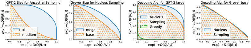
Figure 2: Divergence curves for different models (GPT-2 [45], Grover [61]) and decoding algorithms (greedy decoding, ancestral and nucleus sampling). Mauve is computed as the area of the shaded region, and larger values of Mauve indicate that $Q$ is closer to $P$. In general, Mauve indicates that generations from larger models and nucleus sampling are closer to human text. Rightmost: Nucleus sampling has a slightly smaller Type I error than ancestral sampling but a higher Type II error, indicating that ancestral sampling with Grover base produces more degenerate text while nucleus sampling does not effectively cover the human text distribution.

Summarizing the Errors with a Divergence Curve. Since the mixture weight $\lambda$ was arbitrary, we consider a family of Type I and II error values by varying $\lambda$ between 0 and 1, in the same spirit as information divergence frontiers [49, 16]. This yields a divergence curve,

$$\mathcal{C}(P,Q)=\Big{\{}\big{(}\exp(-c\,{\mathrm{KL}}(Q|R_{\lambda})),\exp(-c\,{\mathrm{KL}}(P|R_{\lambda}))\big{)}\,:\,R_{\lambda}=\lambda P+(1-\lambda)Q,\,\lambda\in(0,1)\Big{\}}\,,$$ (1)

where $c>0$ is a hyperparameter for scaling. The divergence curve formalizes and encodes information about the trade-off between Type I and II errors. Figure 2 illustrates the divergence curves for different models and decoding algorithms.

Our proposed measure, $\textbf{{{{Mauve}}}}(P,Q)$, is the area under the divergence curve $\mathcal{C}(P,Q)$. It provides a scalar summary of the trade-off between Type I and Type II errors. ${{\textsc{Mauve}}}(P,Q)$ lies in $(0,1]$, with a larger value meaning that $Q$ is closer to $P$. Further, ${{\textsc{Mauve}}}(P,Q)=1$ if and only if $Q=P$. The area under the curve is a common summary of trade-off curves in machine learning [13, 11, 12, 19].

Connections to Common Divergences. The divergence curve encodes more information than the KL divergence ${\mathrm{KL}}(P|Q)$, which can be obtained from the second coordinate of the curve $\mathcal{C}(P,Q)$ as $\lambda\to 0$, and the reverse KL divergence ${\mathrm{KL}}(Q|P)$ which can be obtained from the first coordinate of the curve $\mathcal{C}(P,Q)$ as $\lambda\to 1$. Further, the Jensen-Shannon (JS) divergence $\mathrm{JS}(P,Q)=\big{(}{\mathrm{KL}}(P|R_{1/2})+{\mathrm{KL}}(Q|R_{1/2})\big{)}/2$, can be obtained from the two coordinates of $\mathcal{C}(P,Q)$ at $\lambda=1/2$. Mauve summarizes all of the divergence curve $\mathcal{C}(P,Q)$.

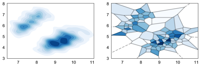
Figure 3: Illustration of the quantization. Left: A continuous two-dimensional distribution $P$. Right: A partitioning of the Euclidean plane $\mathbb{R}^{2}$ and the corresponding quantized distribution $\tilde{P}$.

Computing Mauve for Open-Ended Text Generation. Each point on the divergence curve $\mathcal{C}(P,Q)$ consists of a coordinate

$${\mathrm{KL}}(P|R_{\lambda}) =\sum_{\bm{x}}P(\bm{x})\log\frac{P(\bm{x})}{R_{\lambda}(\bm{x})},$$ (2)

and a similarly defined coordinate ${\mathrm{KL}}(Q|R_{\lambda})$. We cannot compute the summation as written in Eq. (2), as we do not know the ground-truth probabilities $P(\cdot)$ and the support of a typical model distribution is prohibitively large, since it is the space of all sequences of tokens. As a result of these two issues, Mauve cannot be tractably computed in closed form.

We employ a Monte Carlo estimator using samples $\bm{x}_{i}\sim P$ and $\bm{x}_{i}^{\prime}\sim Q$ to overcome the fact that ground-truth probabilities $P(\cdot)$ are unknown. We circumvent the intractable support size by computing Mauve in a quantized embedding space that is sensitive to important features of text.

The overall estimation procedure is as follows. First, we sample human text $\bm{x}_{i}\sim P$ and machine text $\bm{x}_{i}^{\prime}\sim Q$. We then embed each text sequence using an external language model $M$ (e.g., GPT-2 [45]) to obtain embeddings $\{M(\bm{x}_{i})\}_{i=1}^{N}$ and $\{M(\bm{x}_{i}^{\prime})\}_{i=1}^{N^{\prime}}$. Each embedding is now a vector $M(\bm{x})\in\mathbb{R}^{d}$. Next, we jointly quantize the embedded samples (e.g. with $k$-means [36]), and count the cluster assignments to form histograms, giving low-dimensional discrete distributions that approximate each high-dimensional text distribution. In particular, the distribution $P$ of human text is approximated by the discrete distribution $\tilde{P}$ of support size $k$, which is defined as,

$$\tilde{P}(j)=\frac{1}{N}\sum_{i=1}^{N}\mathbb{I}\big{(}\phi(\bm{x}_{i})=j\big{)}\,,$$ (3)

where $\phi(\bm{x})\in\{1,\cdots,k\}$ returns the cluster id of $\bm{x}$. The model distribution $Q$ is approximated as $\tilde{Q}$ similarly. Here, $\tilde{P}$ and $\tilde{Q}$ can be interpreted as piecewise constant approximations of $P$ and $Q$, similar to a histogram; see Figure 3 for an illustration. Computing the divergence curve is now tractable, as each coordinate is a KL divergence between the $k$-element discrete distributions.

To recap, our proposed measure $\textbf{{{{Mauve}}}}{(P,Q)}$ is the area under this divergence curve, providing a summary of all Type I and Type II errors through an efficient approximation designed for text generation. Next, we discuss how Mauve compares to prior comparison measures for text (§3), then present empirical results with Mauve (§4).

3 Related Work

Divergence Measures for Text. Prior measures of similarity/divergence between machine text and human text come in three broad categories: (a) reference-based, (b) statistics-based, and (c) language modeling. Table 1 summarizes the latter two categories, and contrasts them with Mauve.

Reference-based measures evaluate generated text with respect to a (small set of) reference text sample(s), rather than comparing full sequence distributions. These include classical metrics for $n$-gram matching [44, 32, 2], which are designed to capture similarities in the surface form of the generated text and the human references, making them fundamentally ill-suited for open-ended generation. Moreover, it has been recently shown in [42] show that these classical metrics only weakly agree with human judgments.

More recent reference-based metrics are capable of comparisons in a high dimensional space [53, 63, 51, 9], thereby capturing distributional semantics beyond superficial $n$-gram statistics. For instance, Moverscore [64] relies on the Word Mover’s distance [30], and is an instance of an optimal transportation distance [57]. It computes the minimum cost of transforming the generated text to the reference text, taking into account Euclidean distance between vector representations of $n$-grams, as well as their document frequencies. The paradigm of reference-based measures is useful for targeted generation tasks such as translation and summarization where matching a set of references is paramount. It is, however, unsuitable for open-ended generation where there typically are several plausible continuations for each context and creative generations are desirable.

Type	Metric	Measures	Approximates
Statistics	Zipf Coefficient [26]	Unigram rank-frequency statistics	–
	Self-BLEU [65]	N-gram diversity	–
	Generation Perplexity [18]	Generation quality via external model $R$	$|\mathbb{E}_{Q}[\log R(\bm{x})]-\mathbb{E}_{P}[\log R(\bm{x})]|$ (a single point inside $\mathcal{C}(P,Q)$)
Language Modeling	Perplexity	Test-set perplexity	$\mathbb{E}_{P}[\log Q(\bm{x})]$
	$\varepsilon$-perplexity [39]	Perplexity w/ Laplace smoothing	$\mathbb{E}_{P}[\tilde{Q}(\bm{x})]$
	Sparsemax Score [39]	LM quality (sparsemax loss [38])	$\mathbb{E}_{P}[\tilde{Q}(\bm{x})]$
	Token JS-Div. [39]	LM quality (JS divergence)	$\mathbb{E}_{P}[\tilde{Q}(\bm{x})]$
Divergence Curve	Mauve (this work)	Quality & diversity via the divergence curve	$\mathcal{C}(P,Q)$ at all $\lambda$

Table 1: Summary of automatic distributional metrics for evaluating open-ended text generation. Mauve provides a summary of all points along the divergence curve, rather than a single point. The summary is based on comparisons in a joint embedding space, rather than a statistic computed independently on each distribution. $\tilde{Q}$ informally refers to a quantity related to $Q$.

Statistics-based measures compare the model distribution $Q$ with respect to the human distribution $P$ on the basis of some statistic $T(P)$ and $T(Q)$. Property-specific statistics such as the amount of repetition [26, 59], verifiability [40], or termination [58] are orthogonal to Mauve, which provides a summary of the overall gap between $P$ and $Q$ rather than focusing on an individual property. Another statistic is the generation perplexity [18, 26], which compares the perplexity of the model text $\bm{x}\sim Q$ with that of human text $\bm{x}^{\prime}\sim P$ under an external model $R$. By virtue of $T(\cdot)$ being a scalar, generation perplexity cannot trade-off the Type I and Type II errors like Mauve. In fact, we show in Appendix A that the generation perplexity can be derived from a single point enclosed between the divergence curve and the axes.

Language modeling metrics calculate how (un)likely human text $\bm{x}\sim P$ is under the model distribution $Q$, for instance, using the probability $Q(\bm{x})$. These metrics are related to a single point on the divergence curve, rather than a full summary. Examples include the perplexity of the test set (which is a sample from $P$) under the model $Q$ and its generalizations to handle sparse distributions [39]. Unlike Mauve, these metrics never see model text samples $\bm{x}^{\prime}\sim Q$, so they cannot account for how likely the model text is under the human distribution $P$. Moreover, they cannot be used for decoding algorithms such as beam search which do not define a token-level distribution.

Automatic metrics have been proposed for specific domains such as generation of dialogues [55], stories [21], and others [43]. They capture task-specific properties; see the surveys [8, 48]. In contrast, Mauve compares machine and human text in a domain-agnostic manner. Other related work has proposed metrics that rely on multiple samples for quality-diversity evaluation [7], and Bayesian approaches to compare the distribution of statistics in machine translation [17].

Non-automatic Metrics. HUSE [24] aims to combine human judgements of Type I errors with Type II errors measured using perplexity under $Q$. Due to the costs of human evaluation, we consider HUSE, as well other metrics requiring human evaluation, such as single-pair evaluation, as complementary to Mauve, which is an automatic comparison measure. As a separate technical caveat, it is unclear how to use HUSE for sparse $Q$ that assigns zero probability to a subset of text, which is the case with state-of-the-art decoding algorithms [26, 39].

Evaluation of Generative Models. Evaluation of generative models is an active area of research in computer vision, where generative adversarial networks [20] are commonly used. However, metrics such as Inception Score [50] are based on large-scale supervised classification tasks, and thus inappropriate for text generation. The Fréchet Distance [25, 52] and its unbiased counterpart, the Kernel Inception Distance [5] are both used for evaluating generative models, but unlike Mauve, do not take into account a trade-off between different kinds of errors between the learned and a reference distribution. Sajjadi et al. [49] and Kynkäänniemi et al. [31] both proposed metrics based on precision-recall curves. Djolonga et al. [16] proposed information divergence frontiers as a unified framework emcompassing both these works as special cases. Mauve extends the above line of work, and is operationalized for open-ended text generation, applicable for data generated by large-scale neural language models. Complementary to this work, Liu et al. [33] study the theory of information divergence frontiers, proving non-asymptotic bounds on the estimation and quantization error.

4 Experiments

We perform three sets of experiments to validate Mauve. Our first set of experiments (§4.1) examine how known properties of generated text with respect to generation length, decoding algorithm, and model size can be identified and quantified by Mauve. Next, in §4.2 we demonstrate that Mauve is robust to various embedding strategies, quantization algorithms, and hyperparameter settings. Finally, in §4.3 we find that Mauve correlates with human judgments. The code as well as the scripts to reproduce the experiments are available online.

Tasks. We consider open-ended text generation using a text completion task [26, 59] in three domains: web text, news and stories. Each domain consists of a sequence dataset split into (context, continuation) pairs. Given a context $\bm{x}_{1:k}$, the task is to generate a continuation $\hat{\bm{x}}_{k+1:T}\sim Q(\cdot\mid\bm{x}_{1:k})$, forming a completion. Each ground-truth completion $\bm{x}_{1:T}$ is considered a sample from the true distribution $P$, while the completion $(\bm{x}_{1:k},\hat{\bm{x}}_{k+1:T})$ is considered a sample from $Q$. The datasets, context and completion lengths, and number of completions used for each domain are shown in Table 2.

Task Domain Model Finetuning Dataset Prompt Length Max. Generation Length Number of Generations Web text GPT-2 (all sizes) Pretrained Webtext $35$ tokens $1024$ tokens $5000$ News Grover (all sizes) Pretrained RealNews varying $1024$ tokens $5000$ Stories GPT-2 medium Finetuned WritingPrompts $50$ tokens $512$ tokens $5000$

Table 2: Dataset and task summary. Note that $1024$ tokens correspond to $\sim 750$ words on average.

Models. As the language model $\hat{P}(\cdot)$, we use GPT-2, a large-scale transformer [56] pretrained on the web text dataset (see [45]), that is representative of state-of-the-art autoregressive language models. As the embedding model $M(\cdot)$ we use GPT-2 Large, and compare others in §4.2.

Decoding Algorithms. We consider three common decoding algorithms: ancestral sampling which samples directly from the language model’s per-step distributions, $x_{t}\sim\hat{P}(x_{t}\mid\bm{x}_{1:t})$, greedy decoding which selects the most likely next token, $x_{t}=\arg\max_{x\in\mathcal{V}}\hat{P}(x\mid\bm{x}_{1:t})$, as well as nucleus sampling [26] which samples from top-$p$ truncated per-step distributions, $x_{t}\sim\hat{P}_{\text{nuc},p}(x_{t}\mid\bm{x}_{1:t})$, which is defined as

$$\hat{P}_{\text{nuc},p}(x_{t}\mid\bm{x}_{1:t})\propto\begin{cases}\hat{P}_{\text{nuc},p}(x_{t}\mid\bm{x}_{1:t}),&\text{if }x_{t}\in V_{p},\\ 0,&\text{else}.\end{cases}$$

Here, the top-$p$ vocabulary $V_{p}$ is the smallest set $V$ such that $\sum_{x\in V}\hat{P}(x\mid\bm{x}_{1:t})\geq p$.

We also consider an adversarial sampling procedure, designed to generate low-quality text that nevertheless matches the perplexity of human text. Adversarial perplexity sampling proceeds in two phases: (1) we generate the first 15% of tokens in a sequence uniformly at random from the vocabulary, and (2) we generate the remaining tokens greedily to make the running perplexity of the generated sequence as close as possible to the perplexity of human text.

4.1 Quantifying Properties of Generated Text

To study Mauve’s effectiveness as a measure for comparing text distributions, we first examine how Mauve quantifies known properties of generated text: a good measure should meet expected behavior that is known from existing research on each property. Specifically, we investigate how Mauve behaves under changes in generation length, decoding algorithm, and model size.

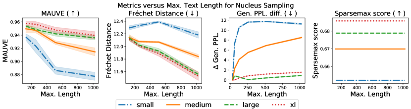
Figure 4: Generation quality versus maximum generation length according to Mauve and three alternative measures (web text, GPT-2). Mauve is the only comparison measure which identifies that generation quality decreases monotonically with increasing text length. The shaded area shows one standard deviation over generations from 5 random seeds.

Mauve quantifies quality differences due to generation length. Although large transformer-based models can generate remarkably fluent text, it has been observed that the quality of generation deteriorates with text length: as the generation gets longer, the model starts to wander, switching to unrelated topics and becoming incoherent [46]. As a result, an effective measure should indicate lower quality (e.g. lower Mauve) as generation length increases.

Figure 4 shows Mauve as the generation length increases, along with three alternative metrics: generation perplexity, sparsemax score, and Fréchet distance [25, 52]. Mauve reflects the desired behavior, showing a decrease in quality (lower Mauve) as generation length grows, with the trend consistent across model sizes. The other three metrics, however, show less favorable trends. Fréchet distance indicates improving quality as the length increases, while generation perplexity shows non-monotonic quality trends for the small and large models. Finally, language modeling metrics such as the sparsemax score [39] remain constant, since they do not depend on the samples generated.

Mauve identifies quality differences between decoding algorithms. Recent work has identified two clear trends in open-ended text generation with standard autoregressive models: (1) using greedy decoding results in repetitive, degenerate text [26, 59, 58]; (2) nucleus sampling (and related truncated sampling methods) yields higher quality text than ancestral sampling [18, 26]. An effective measure should thus indicate the quality relationship $\text{greedy}\prec\text{ancestral}\prec{\text{nucleus}}$.

Table 4 summarizes Mauve’s quality measures of greedy decoding, ancestral sampling, and nucleus sampling, along with alternative automated metrics and a human quality score. Mauve correctly identifies the expected quality relationship, assigning the lowest quality to greedy decoding ($.016$) followed by ancestral sampling ($.882$), and the highest quality to nucleus sampling ($.940$). Other commonly-used metrics fail to identify this relationship: generation perplexity rates the highly degenerate greedy-decoded text as better than ancestral sampling ($11.324$ vs. $19.284$), while the language-modeling metrics (SP, JS, $\varepsilon$-PPL) rate nucleus-decoded text as equal to or worse than greedy decoding or ancestral sampling. Further, as we show in Appendix D, Mauve rightly identifies degeneracy of beam search, thus quantifying the qualitative observations of Holtzman et al. [26]. Finally, generation perplexity falls victim to the adversarial decoder (Adv.), unlike Mauve.

Mauve quantifies quality differences due to model size. Scaling the model size has been a key driver of recent advances in NLP, with larger models leading to better language modeling and higher quality generations in open-ended settings [45, 6]. An effective metric should capture the relationship between model size and generation quality, which we verify with human quality scores.

Table 4 shows Mauve’s quality measures as the model size increases, along with alternatives and human quality scores. Mauve increases as model size increases, agreeing with the human quality measure and the expectation that larger models should have higher quality generations. The widely-used generation perplexity, however, incorrectly rates the large model’s text as the best. Although the language modeling metrics (SP, JS, and $\varepsilon$-PPL) capture the size-quality relationship, they are constant with respect to length (Figure 4), and did not correctly quantify decoding algorithm quality (Table 4).

Table 6 in Appendix D shows additional results with ancestral sampling. In this case, human evaluators rated generations from the small model as better than those from the medium model. Interestingly, Mauve also identified this relationship, agreeing with the human ratings, in contrast to the other automatic metrics we surveyed.

	Adv.	Greedy	Sampling	Nucleus
Gen. PPL($\downarrow$)	lightmauve!30$\mathbf{0.05}$	$11.3$	$19.3$	$1.54$
Zipf($\downarrow$)	$0.03$	$0.02$	$0.02$	lightmauve!30$\mathbf{0.01}$
Self-BLEU($\downarrow$)	$0.07$	$0.03$	lightmauve!30$\mathbf{0.02}$	$0.03$
SP($\uparrow$)	–	$0.50$	lightmauve!30$\mathbf{0.69}$	$0.69$
JS($\downarrow$)	–	lightmauve!30$\mathbf{0.35}$	$0.37$	$0.36$
$\varepsilon$-PPL($\downarrow$)	–	$497$	lightmauve!30$\mathbf{11.4}$	$13.7$
Mauve ($\uparrow$)	$0.06$	$0.02$	$0.88$	lightmauve!30$\mathbf{0.94}$
Human($\uparrow$)	–	–	$9.0$	lightmauve!30$\mathbf{15.7}$

Table 3: Generation quality w.r.t different decoding algorithms (web text, GPT-2 xl) under various metrics, and humans. Mauve correctly captures the relationship $\text{greedy}\prec\text{ancestral}\prec{\text{nucleus}}$, and rates the adversarial decoder’s text as low quality. Results are consistent across model sizes and random seeds. Boldfaced/highlighted entries denote the best decoding algorithm under each metric.

	Small	Medium	Large	XL
Gen. PPL($\downarrow$)	$11.2$	$8.5$	lightmauve!30$\mathbf{0.9}$	$1.5$
Zipf($\downarrow$)	$0.06$	lightmauve!30$\mathbf{0.00}$	$0.02$	$0.01$
Self-BLEU($\downarrow$)	$0.05$	lightmauve!30$\mathbf{0.02}$	$0.03$	$0.03$
SP($\uparrow$)	$0.65$	$0.67$	$0.68$	lightmauve!30$\mathbf{0.69}$
JS($\downarrow$)	$0.41$	$0.39$	$0.37$	lightmauve!30$\mathbf{0.36}$
$\varepsilon$-PPL($\downarrow$)	$25.9$	$18.8$	$14.9$	lightmauve!30$\mathbf{13.7}$
Mauve ($\uparrow$)	$0.878$	$0.915$	$0.936$	lightmauve!30$\mathbf{0.940}$
Human($\uparrow$)	$-15.9$	$-3.4$	$12.6$	lightmauve!30$\mathbf{15.7}$

Table 4: Generation quality w.r.t different model sizes (web text, nucleus sampling) under various metrics, as well as human evaluators. Mauve captures the relationship between model size and generation quality, agreeing with human-evaluated quality. Results are consistent across random seeds and decoding algorithms. Boldfaced/highlighted entries denote the best model size under each metric.

Summary. Mauve identifies properties of generated text that a good measure should capture, related to length, decoding algorithm, and model size. In contrast, commonly used language modeling and statistical measures did not capture all of these properties. Unlike these alternatives, which capture a single statistic or relate to a single point on the divergence curve, Mauve’s summary measure incorporates type I errors that quantify the degenerate text produced by greedy decoding (recall Figure 1), while capturing distribution-level information that describes quality changes from generation length, model size, and the nuanced distinction between ancestral and nucleus sampling.

4.2 Approximations in Mauve

Mauve summarizes the divergence between two text distributions with an approximation that relies on two components: an embedding model $M(\bm{x})$ and a quantization algorithm $\mathcal{A}$ (§2, Eq. (3)). We study the effects of these two components.

Mauve works with alternative embedding models. Figure 5 (left) shows that Mauve with features from RoBERTa- large [34] gives qualitatively similar trends across model size and decoding as Mauve with features from GPT-2 large. Quantitatively, the Spearman rank correlation between them across all model and decoders is $0.993$. We observe that RoBERTa penalizes smaller models more than GPT-2 but rates greedy decoding higher. We leave further study of inductive biases in the different embedding models to future work.

Mauve is robust to quantization. We compare different three different quantization algorithms:

1. $k$-Means: We cluster the hidden representations using $k$-means, and represent them by their cluster membership to get a discrete distribution with size equal to the number of clusters.

2. Deep Residual Mixture Models (DRMM): As a generalization of $k$-means, we train a deep generative model known as DRMM [22]. We convert the soft clustering returned by DRMM into a hard clustering by assigning each point to its most likely cluster, and quantize the data using the cluster membership. We use DRMM with $3$ layers and $10$ components per layer for a total of $10^{3}$ clusters, and train it for $20$ epochs.

3. Lattice Quantization: We learn a $4$-dimensional feature representation of the vectors $M(\bm{x})$ using a deep network which maintains the neighborhood structure of the data while encouraging the features to be uniformly distributed on the unit sphere [47]. We quantize the data on a uniform lattice into $744$ bins.

We compare different choices of the quantization to $k$-means with $k=500$, which is our default. The Spearman rank correlation between Mauve computed with $k$-means for $k$ ranging from $100$ to $5000$ correlates nearly perfectly with that of $k=500$. In particular, the Spearman correlation is exactly $0.99$ or $1.00$. Likewise, Mauve computed with DRMM or lattice quantization has a near-perfect Spearman correlation of at least $0.99$ with $k$-means. While the actual numerical value of Mauve could vary with the quantization algorithm, these results show that the rankings induced by various variants of Mauve are nearly identical.

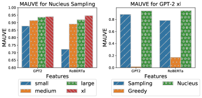
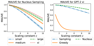
Figure 5: Left: Mauve computed using GPT-2 (default) and RoBERTa [34] embeddings, across model sizes and decoding algorithms; see Table 12 in the Appendix for further results. The Spearman rank correlation between the two is 0.993 across model sizes and decoding algorithms. Right: Effect of the scaling constant $c$ on Mauve. Choice of $c$ does not affect the relative order of the curves but only the numerical value. We use $c=5$ to get interpretable values with both nucleus and greedy decoding.

Practical recommendation for scaling parameter. Figure 5 (right) shows the effects of adjusting the scaling parameter $c$, which does not affect the relative order of the divergence curve, but adjusts the numerical value returned by Mauve. As a practical recommendation, we found $c=5$ to yield interpretable values.

4.3 Correlation with Human Judgments

An effective metric should yield judgments that correlate highly with human judgments, assuming that human evaluators represent a gold-standard. We evaluate how Mauve’s quality judgments correlate with human quality judgments. In our study, a quality judgment means choosing a particular (model, decoder) setting based on the resultant generations.

Evaluation Protocol. To obtain human judgments, we employ a pairwise setup: at each round, an annotator receives a context and continuations from two different (model, decoder) settings, and selects the continuation they found more natural using a 5-point Likert scale. Our interface for collecting annotations is shown in Figure 9 of Appendix E, which also includes further details and additional results.

We collect these annotations for web text generation with 8 different (model, decoder) settings plus a ninth setting for human-written continuations. Each setting is a GPT-2 model size paired with either ancestral or nucleus sampling. This gives us a total of $36$ pairs of settings. Given the known difficulties with human evaluation of longer texts [28], we use a maximum completion length of $256$ tokens. We obtain $90$ preference ratings for each pair of settings, coming from a total of $214$ crowd-workers from the Amazon Mechanical Turk platform. The evaluators were paid USD $0.40$ per evaluation based on an estimated wage of USD $16$ per hour.

We convert these pairwise preferences to a ranking by fitting a Bradley-Terry model [37], a parametric model used to predict the outcome of a head-to-head comparison. In particular, we obtain a score $w_{i}$ for each setting $i$ so that the log odds of humans preferring setting $i$ to setting $j$ in a head-to-head comparison is given by the difference $w_{i}-w_{j}$. For a given comparison measure, we compute the Spearman rank correlation between the comparison measure and the fitted Bradley-Terry coefficients $w_{i}$ for each of the (model, decoder) settings. The end result is a correlation score in $[-1,1]$, with higher values meaning that quality judgments using the comparison measure correlate with quality judgments made by human evaluators.

Mauve correlates with human judgments. Table 5 shows the correlation between human judgments and five automatic evaluation metrics obtained using our evaluation protocol on the web text domain. Mauve correlates highly with human judgments of how human-like ($0.952$), interesting $(0.810)$, and sensible $(0.857)$ the machine text is. Mauve’s correlations with human judgments are substantially higher than those for the other automated measures; for instance, the commonly-used generation perplexity has correlations that are $0.12$ to $0.17$ lower than Mauve’s. The results suggest that Mauve may act as an effective, automatic surrogate for costly human judgments.

Metric Task Gen. PPL Zipf Coef. REP Distinct-4 Self-BLEU Mauve Human-like/BT Web text $0.810$ $0.833$ $-0.167$ $0.738$ $0.595$ lightmauve!30$\mathbf{0.952}$ Interesting/BT Web text $0.643$ $0.524$ $-0.143$ $0.524$ $0.405$ lightmauve!30$\mathbf{0.810}$ Sensible/BT Web text $0.738$ $0.690$ $-0.071$ $0.595$ $0.524$ lightmauve!30$\mathbf{0.857}$ % Disc. Acc. News $0.468$ $0.595$ $0.792$ $0.653$ $0.516$ lightmauve!30$\mathbf{0.956}$ % Disc. Acc. Stories $0.643$ $0.643$ $0.250$ $0.750$ $0.857$ lightmauve!30$\mathbf{0.893}$

Table 5: Correlation of various similarity measures with human judgments when available, and the accuracy of a trained discriminator otherwise. “BT” denotes the Bradley-Terry score for a pairwise human evaluation (§ 4.3). Boldfaced/highlighted numbers indicate highest correlation in each row. We observe that Mauve has the highest correlation with human evaluation and discriminator accuracy.

Mauve correlates with learned discriminators. We also measure the quality of generations by how well a trained model (a discriminator) can distinguish between real and generated text [35]. We report the test accuracy of a binary classifier trained to discriminate between machine and human text; a lower discrimination accuracy implies that the generation is harder to distinguish from human text. We report the accuracy of Grover mega as the discriminator for the news generations as it produced the highest discrimination accuracy [61] while we use GPT-2 large for the story domain. As seen in Table 5, Mauve correlates the highest with the discrimination accuracy ($0.96$ for news and $0.89$ for stories) among all comparison measures. Computing the discrimination accuracy for each (model, decoder) pair requires fine-tuning a separate model, which is particularly expensive for large models such as Grover-mega. Mauve, on the other hand, does not require any training.

5 Conclusion

We presented Mauve, an automatic measure of the gap between neural text and human text for open-ended text generation. Mauve measures the area under a divergence curve, formalizing and summarizing a spectrum of errors that capture phenomena present in machine and human-generated text. Mauve correlated with human judgments and identified quality differences due to generation length, decoding algorithm, and model size, which prior metrics struggle to capture. Automated metrics have driven advances in computer vision and many other machine learning domains. Mauve’s principled foundation and strong empirical performance offers a similar path forward for open-ended text generation systems. Extensions of Mauve to closed-ended tasks, such as summarization and translation, where generations must be compared to a fixed set of gold-standard references, are promising directions for future work.

Broader Impacts Statement

Mauve rewards model text which resembles human-authored text. However, we acknowledge the risks of rewarding systems that try to mimic humans [4], which is the ultimate goal of open-ended text generation. While our research is important for developing better language generators, we also encourage the community to pay attention to the development of technology that can reliably distinguish between human and machine text. We leave the extension of our method towards building such systems to future work.

Acknowledgments

Part of this work was done while Zaid Harchaoui was visiting the Simons Institute for the Theory of Computing, and while John Thickstun was at the University of Washington. This work was supported by NSF DMS-2134012, NSF CCF-2019844, NSF DMS-2023166, the DARPA MCS program through NIWC Pacific (N66001-19-2-4031), the CIFAR “Learning in Machines & Brains” program, a Qualcomm Innovation Fellowship, and faculty research awards.

Appendix

Appendix A Divergence Curves and Mauve: Additional Details

We discuss some aspects of the divergence curves alluded to in §2 and §3. In particular, we discuss the following.

• Appendix A.1: the Pareto optimality of the divergence curves, mentioned in a footnote in §2.

• Appendix A.2: the connection between generation perplexity and the divergence curves as mentioned in §3.

• Appendix A.3: a formal definition of the quantization which is first introduced in §2, as well as an illustration.

• Appendix A.4: the pesudocode for Mauve.

A.1 Pareto Optimality of Divergence Curves

Here, we show the property of Pareto optimality of $\mathcal{C}(P,Q)$. We refer to the textbook [23] for more background on information theory and KL divergence. The main property we will show in this section is the following.

Proposition 1.

Consider two distributions $P,Q$ with finite support and a scaling constant $c>0$. Let $R_{\lambda}$ be such that $\big{(}e^{-c\,{\mathrm{KL}}(Q|R_{\lambda})},e^{-c\,{\mathrm{KL}}(P|R_{\lambda})}\big{)}\in\mathcal{C}(P,Q)$. Then, $R_{\lambda}$ is Pareto-optimal for the pair of objectives $\big{(}{\mathrm{KL}}(Q|\cdot),{\mathrm{KL}}(P|\cdot)\big{)}$. In other words, there does not exist any distribution $R$ such that ${\mathrm{KL}}(Q|R)<{\mathrm{KL}}(Q|R_{\lambda})$ and ${\mathrm{KL}}(P|R)<{\mathrm{KL}}(P|R_{\lambda})$ simultaneously.

Proof.

Let $\mathcal{F}(P,Q)$ be the Pareto frontier of $\big{(}{\mathrm{KL}}(Q|\cdot),{\mathrm{KL}}(P|\cdot)\big{)}$. The convexity of ${\mathrm{KL}}(Q|\cdot),{\mathrm{KL}}(P|\cdot)$ allows us to compute the Pareto frontier $\mathcal{F}(P,Q)$ exactly by minimizing linear combinations of the objectives. Concretely, we have from [41, Thm. 3.4.5, 3.5.4] that

$$\mathcal{F}(P,Q)=\Big{\{}\big{(}{\mathrm{KL}}(P|R_{\lambda}^{\star}),{\mathrm{KL}}(P|R_{\lambda}^{\star})\big{)}\,:\,\lambda\in[0,1]\Big{\}}$$

where

$$R_{\lambda}^{\star}\in\operatorname*{arg\,min}_{R}\{\lambda\,{\mathrm{KL}}(Q|R)+(1-\lambda){\mathrm{KL}}(P|R)\}\,.$$

We invoke the next lemma to show that $R_{\lambda}^{\star}=\lambda P+(1-\lambda)Q$ to complete the proof. ∎

Lemma 2.

Let $P,Q,S$ be discrete distributions with finite support. For any $\lambda\in[0,1]$ and $\bar{\lambda}=1-\lambda$, letting $R_{\lambda}=\lambda P+\bar{\lambda}Q$, we have the identity

$$\lambda\,{\mathrm{KL}}(P|S)+\bar{\lambda}\,{\mathrm{KL}}(Q|S)=\lambda\,{\mathrm{KL}}(P|R_{\lambda})+\bar{\lambda}\,{\mathrm{KL}}(Q|R_{\lambda})+{\mathrm{KL}}(R_{\lambda}|S)\,.$$

Consequently, we have that

$$R_{\lambda}\in\operatorname*{arg\,min}_{S}\left\{\lambda\,{\mathrm{KL}}(P|S)+\bar{\lambda}\,{\mathrm{KL}}(Q|S)\right\}\,.$$

Proof.

By adding and subtracting $\sum_{i}R_{\lambda,i}\log(R_{\lambda,i})$, we get,

$$\lambda\,{\mathrm{KL}}(P|S)+\bar{\lambda}\,{\mathrm{KL}}(Q|S) =\sum_{i}\lambda P_{i}\log P_{i}+\bar{\lambda}Q_{i}\log Q_{i}-R_{\lambda,i}\log S_{i}$$

$$=\sum_{i}\lambda P_{i}\log\frac{P_{i}}{R_{\lambda,i}}+\bar{\lambda}Q_{i}\log\frac{Q_{i}}{R_{\lambda,i}}+R_{\lambda,i}\log\frac{R_{\lambda,i}}{S_{i}}$$

$$=\lambda\,{\mathrm{KL}}(P|R_{\lambda})+\bar{\lambda}\,{\mathrm{KL}}(Q|R_{\lambda})+{\mathrm{KL}}(R_{\lambda}|S)\,.$$

The first two terms are independent of $S$ and the last term is minimized at $S=R_{\lambda}$. ∎

Connection to Divergence Frontiers [16]. The Pareto frontier $\mathcal{F}(P,Q)$ of $\big{(}{\mathrm{KL}}(Q|\cdot),{\mathrm{KL}}(P|\cdot)\big{)}$ (defined in the proof of Proposition 1) coincides exactly with the notion of the inclusive divergence frontier, as defined by Djolonga et al. [16]. It follows that the inclusive KL divergence frontier is related to the divergence curve we have defined as,

$$\mathcal{F}(P,Q)=\Big{\{} \left(c^{-1}\log t_{1}^{-1},c^{-1}\log t_{2}^{-1}\right)\,:\,(t_{1},t_{2})\in\mathcal{C}(P,Q)\Big{\}}\,.$$

A.2 Generation Perplexity and Divergence Curves

Recall that the generation perplexity of a text distribution $P$ is the perplexity of this distribution under an external language model $R$. That is,

$$T_{\text{ppl}}(P)=\exp\left(-\mathbb{E}_{P}[\log R(\bm{x})]\right)\,.$$

For simplicity, we write the perplexity using base $e$ rather than base $2$. Then, the difference in generation perplexity between $P$ and $Q$ is given by

$$\big{|}T_{\text{ppl}}(P)-T_{\text{ppl}}(Q)\big{|} =\Big{|}\exp\big{(}-\mathbb{E}_{P}[\log R(\bm{x})]\big{)}-\exp\big{(}-\mathbb{E}_{Q}[\log R(\bm{x})]\big{)}\Big{|}$$

$$=\Big{|}\exp\big{(}H(P)+{\mathrm{KL}}(P|R)\big{)}-\exp\big{(}H(Q)+{\mathrm{KL}}(Q|R)\big{)}\Big{|}\,,$$

where $H(P)=-\mathbb{E}_{P}[\log P(\bm{x})]$ is the Shannon entropy of $P$. When $H(P)=H(Q)=\log C$, i.e., both $P$ and $Q$ are equally diverse, then

$$\big{|}T_{\text{ppl}}(P)-T_{\text{ppl}}(Q)\big{|}=C\,\Big{|}\exp\big{(}{\mathrm{KL}}(P|R)\big{)}-\exp\big{(}{\mathrm{KL}}(Q|R)\big{)}\Big{|}\,.$$

When $R=\lambda P+(1-\lambda)Q$, this is proportional to the difference between the reciprocal of two coordinates of one point on the divergence curve. When $R$ is some other model, then $\big{(}\exp(-{\mathrm{KL}}(Q|R)),\exp(-{\mathrm{KL}}(P|R))\big{)}$ corresponds to the coordinates of a point enclosed within the divergence curve and the coordinate axes. Indeed, this is because the divergence curve encodes the Pareto frontier of $({\mathrm{KL}}(P|\cdot),{\mathrm{KL}}(Q|\cdot))$.

When $H(P)\neq H(Q)$, the difference in the generation perplexity can be written as a function of some point $\big{(}\exp(-{\mathrm{KL}}(Q|R)),\exp(-{\mathrm{KL}}(P|R))\big{)}$ that is enclosed within the divergence curve and the axes:

$$\big{|}T_{\text{ppl}}(P)-T_{\text{ppl}}(Q)\big{|}=\Big{|}C_{1}\,\exp\big{(}{\mathrm{KL}}(P|R)\big{)}-C_{2}\,\exp\big{(}{\mathrm{KL}}(Q|R)\big{)}\Big{|}\,,$$

where $C_{1}=\exp(H(P))$ and $C_{2}=\exp(H(Q))$.

A.3 Quantization: Definition

We formally define the quantization of a distribution.

Consider a distribution $P$ over some space $\mathcal{X}$. Consider a partition $S=(S_{1},\cdots,S_{k})$ of $\mathcal{X}$, i.e., $\cup_{j=1}^{k}S_{j}=\mathcal{X}$ and $S_{i}\cap S_{j}=\varnothing$ if $i\neq j$. Quantizing the distribution $P$ over partitions $S$ gives us a multinomial distribution $\tilde{P}_{S}$ over $k$ elements. Concretely, we have,

$$\tilde{P}_{S}(j)=P(S_{j})\,.$$

This histogram is a classical example of a quantizer. While the quantized distribution $\tilde{P}_{S}$ is a discrete multinomial distribution, it can be viewed as a piecewise constant approximation to $P$, similar to the histogram. This is visualized in Figure 3 for a two-dimensional example. In our setting, $\mathcal{X}$ is the space of encoded representation of text, i.e., a Euclidean space $\mathbb{R}^{d}$. We use data-dependent quantization schemes such as $k$-means and lattice quantization of a learned feature representation. In one-dimension, quantization is equivalent to computing a histogram. Hence, we casually use the term “bin” to refer to a partition.

A.4 Pseudocode for Mauve

Algorithm 1 shows the pseudocode for computing Mauve. It consists of the following steps:

• The first step is to embed the sampled text using an external language model $M$. In our experiments, we use GPT-2 large [45].

• The second step is to quantize the embeddings. We primarily use $k$-means, which returns the cluster memberships $C_{P}$ and $C_{Q}$.

• The third step is to form the quantized distributions from the cluster memberships from (3). This amounts to counting the number of points in each cluster contributed by $P$ and $Q$.

• The next step is to build the divergence curve. The full divergence curve (1) is a continuously parameterized curve for $\lambda\in(0,1)$. For the sake of computation, we take a discretization $\Lambda$ of $[0,1]$:

  $$\hat{\mathcal{C}}(P,Q)=\Big{\{}\big{(}\exp(-c\,{\mathrm{KL}}(Q|R_{\lambda})),\exp(-c\,{\mathrm{KL}}(P|R_{\lambda}))\big{)}\,:\,\begin{matrix}R_{\lambda}=\lambda P+(1-\lambda)Q,\\ \lambda\in\Lambda\end{matrix}\Big{\}}\,.$$ (4)

  We take a uniform grid $\Lambda=\{1/n,2/n,\cdots,(n-1)/n\}$ with $n$ points.

• The last step is to estimate the area under $\hat{\mathcal{C}}(\tilde{P},\tilde{Q})$ using numerical quadrature.

Input: Human text $\{\bm{x}_{i}^{P}\}_{i=1}^{N}$, model text $\{\bm{x}_{i}^{Q}\}_{i=1}^{N^{\prime}}$, number of clusters $k$, embedding model $M$, discretization $\Lambda$ of $[0,1]$.

Output: ${{\textsc{Mauve}}}(P,Q)$.

 // Embed the samples

$\{M(\bm{x}_{i}^{P})\}_{i=1}^{N}$, $\{M(\bm{x}_{i}^{Q})\}_{i=1}^{N^{\prime}}\leftarrow\texttt{embed}\left(M,\{\bm{x}_{i}^{P}\}_{i=1}^{N},\{\bm{x}_{i}^{Q}\}_{i=1}^{N^{\prime}}\right)$

 // Cluster embeddings jointly

$C_{P},C_{Q}=\texttt{quantize}\left(\{M(\bm{x}_{i}^{P})\}_{i=1}^{N},\{M(\bm{x}_{i}^{Q})\}_{i=1}^{N^{\prime}}\right)$

 // Form quantized distributions by counting cluster assignments

$\tilde{P}\leftarrow\texttt{count}(C_{P})/N$,   $\tilde{Q}\leftarrow\texttt{count}(C_{Q})/N^{\prime}$

 // Build the divergence curve

Compute $\hat{\mathcal{C}}(\tilde{P},\tilde{Q})$ from (4) for $\lambda\in\Lambda$

 // Compute Mauve using numerical quadrature

return $\texttt{area}\left(\hat{\mathcal{C}}(\tilde{P},\tilde{Q})\right)$

Algorithm 1 Pseduocode to compute Mauve

Appendix B Software Package

We illustrate the use of the accompanying Python package, available on GitHub and installable via pip as pip install mauve-text.

Listing 1: Compute Mauve from text

⬇

1from mauve import compute_mauve

2

3p_text = ... # list of strings representing human distribution P

4q_text = ... # list of strings representing model distribution Q

5

6# Obtain feature representation, quantize it and then compute MAUVE

7out = compute_mauve(p_text=p_text, q_text=q_text,

8 device_id=0, # use GPU 0 for featurization

9 max_text_length=256 # truncate text to 256 tokens

10 )

11print(’MAUVE(P, Q) =’, out.mauve)

12

13# Plot the divergence curve

14import matplotlib.pyplot as plt

15plt.plot(out.divergence_curve[:, 0], out.divergence_curve[:, 1])

16

17# Visualize quantized versions of P and Q

18import numpy as np

19idxs = np.argsort(out.p_hist)[::-1]

20sample_p = np.random.multinomial(n=1000, pvals=out.p_hist[idxs])

21sample_q = np.random.multinomial(n=1000, pvals=out.q_hist[idxs])

22

23x = np.arange(out.p_hist.shape[0])

24plt.bar(x, sample_p, color=’blue’, alpha=0.3, label=’P’)

25plt.bar(x, sample_q, color=’red’, alpha=0.3, label=’Q’)

26plt.legend()

Appendix C Experiments: Setup

Here, we provide the full details of the experiments in §4. In particular, the outline of this appendix is as follows.

• Appendix C.1: the three task domains considered in the expeirments.

• Appendix C.2: training and decoding hyperparameters for each of these tasks.

• Appendix C.3: hyperparameters of Mauve.

• Appendix C.4: details of other automatic comparison measures we consider.

• Appendix C.5: other details (software, hardware, running time, etc.).

C.1 Task Domains

We consider an open-ended text generation task under three domains: web text, news and stories. As summarized in Table 2, we follow a slightly different setting for the task in each domain:

Web text Generation. The goal of this task is to generate articles from the publicly available analogue of the Webtext dataset using pretrained GPT-2 models for various sizes. At generation time, we use as prompts the first $35$ tokens of each of the $5000$ articles from the Webtext test set, keeping maximum generation length to $1024$ tokens (which corresponds, on average, to around $750$ words). For comparison with human text, we use the corresponding human-written continuations from the test set (up to a maximum length of $1024$ tokens).

News Generation. Under this task, the goal is to generate the body of a news article, given the title and metadata (publication domain, date, author names). We use a Transformer-based [56] causal language model, Grover [61], which is similar to GPT-2, but tailored to generating news by conditioning on the metadata of the article as well. Our generations rely on pretrained Grover architectures of various sizes. The generation prompt comprises the headline and metadata of $5000$ randomly chosen articles from the April2019 set of the RealNews dataset [61], and the maximum article length was $1024$ tokens. We reuse the publicly available Grover generations for our evaluation.

Story Continuation. Given a situation and a (human-written) starting of the story as a prompt, the goal of this task is to continue the story. Here, we use a GPT-2 medium model fine-tuned for one epoch on the WritingPrompts dataset [18]. We use as generation prompts the first $50$ tokens of $5000$ randomly chosen samples of the test set of WritingPrompts. The machine generations are allowed to be up to $512$ tokens long. The corresponding test examples, truncated at $512$, tokens are used as human-written continuations.

C.2 Training and Decoding Hyperparameters

We use size-based variants of Transformer language models [56] for training each task (domain). At decoding time, we explore a text continuation setting, conditioned on a prompt containing human-written text. All experiments were built using pretrained (and if applicable, finetuned) models implemented in the HuggingFace Transformers library [60]. The tasks are summarized in Table 2.

Story Continuation Finetuning. We finetune GPT-2 medium on the training set of the WritingPrompts dataset using the cross entropy loss for one epoch over the training set with an effective batch size of $32$ and a block size of $512$. We use the default optimizer and learning rate schedules of the HuggingFace Transformers library, i.e., the Adam optimizer with a learning rate of $5\times 10^{-5}$.

Decoding Hyperparameters. We consider pure sampling (i.e., ancestral sampling from the model distribution), greedy decoding (i.e., choosing the argmax token recursively), and nucleus sampling [26] with parameter $p\in\{0.9,0.92,0.95,0.99\}$ for web text generation and story continuation, and $p\in\{0.9,0.92,0.94,0.96,0.98\}$ for news generation.

C.3 Mauve Hyperparameters

Mauve’s hyperparameters are the scaling constant $c$, the embedding model $M$, and the quantization algorithm (including the size of the quantized distribution).

C.3.1 Scaling Constant

Note that Mauve’s dependence on $c$ is order-preserving since the map $x\mapsto\exp(-cx)$ is strictly monotonic in $x$. That is, if ${{\textsc{Mauve}}}_{c_{1}}(P,Q_{1})>{{\textsc{Mauve}}}_{c_{1}}(P,Q_{2})$, then it holds that ${{\textsc{Mauve}}}_{c_{2}}(P,Q_{2})>{{\textsc{Mauve}}}_{c_{2}}(P,Q_{2})$ for all scaling constants $c_{1},c_{2}>0$. In other words, the choice of the scaling constant affects the numerical value of Mauve but leaves the relative ordering between different models unchanged. We choose $c=5$ throughout because it allows for a meaning comparison between the numerical values of Mauve; Appendix D.3 gives the values of Mauve for various values of $c$.

C.3.2 Embedding Model

We compute text embeddings from the GPT-2 large model. We find in Appendix D.3 that feature representations obtained from other large transformer models such as RoBERTA [34] also achieves similar results.

C.3.3 Quantization

We experiment with three quantization algorithms.

Mauve-$k$-means. We first run PCA on the data matrix obtained from concatenating the hidden state representations of the human text and model text. We keep $90\%$ of the explained variance and normalize each datapoint to have unit $\ell_{2}$ norm. We then run $k$-means with FAISS for a maximum of $500$ iterations for $5$ repetitions; the repetition with the best objective value is used for the quantization. We quantize the human text distribution and the model text distribution by a histogram obtained from cluster memberships. We vary the number of clusters in $\{100,250,500,1000\}$. Too few clusters makes the distributions seem closer than they actually are while too many clusters leads to many empty clusters (which makes all distributions seem equally far away). Yet, we find in Appendix D.3 that Mauve with all these values of $k$ correlate strongly with each other; we use as default $k=500$ clusters as it is neither too small nor too large.

Mauve-DRMM. We use the code released by the authors of [22]. We take $10$ components per layer and $3$ layers for a total of $1000$ components. We train the DRMM for $20$ epochs using the hyperparameters suggested by the authors, i.e., a batch size of $64$ with a learning rate

$$\gamma_{t}=\gamma_{0}\min\{1,(2-2t/T)^{2}\}\,,$$

where $T$ is the total number of updates and the initial learning $\gamma_{0}=0.005$. That is, the learning rate is set to a constant for the first half of the updates and then annealed quadratically. For more details, see [22, Appendix C].

Mauve-Lattice. We use the code provided by the authors of [47]. We train a $4$-dimensional feature representation of the hidden states for for $200$ epochs using the triplet loss of [47], so that the learnt feature representations are nearly uniformly distributed. We use a $2$-layer multilayer perceptron with batch normalization to learn a feature representation. We train this MLP for $200$ epochs with hyperparameters suggested by the authors, i.e., a batch size of $64$ and an initial learning rate of $0.1$. The learning rate is cut to $0.05$ after half the training and $0.01$ after $75\%$ of the training.

The learnt feature representations are then quantized using the lattice spherical quantizer into $744$ bins. This work as follows: let $S_{r}$ denote the integral points of the unit sphere of radius $r=\sqrt{50}$ in $\mathbb{R}^{4}$. A hidden state vector $x$ is run through the trained MLP $f$ to get its feature representation $f(x)$. Next, $f(x)$ is quantized to $\operatorname*{arg\,min}_{u\in S_{r}}\left\|f(x)-{u}/{r}\right\|_{2}^{2}$.

C.4 Automatic Comparison Measures: Details and Hyperparameters

We now describe the other automatic comparison measures we compared Mauve to, as well as their hyperparameters.

• Generation Perplexity (Gen. PPL.): We compute the perplexity of the generated text under the GPT-2 large model.

• Zipf Coefficient: we report the slope of the best-fit line on log-log plot of a rank versus unigram frequency plot. Note that the Zipf coefficient only depends on unigram count statistics and is invariant to, for instance, permuting the generations. We use the publicly available implementation of [26].

• Repetition Frequency (Rep.): The fraction of generations which devolved into repetitions. Any generation which contains at least two contiguous copies of the same phrase of any length appearing at the end of a phrase is considered a repetition. We consider repetitions at the token level.

• Distinct-$n$: The fraction of distinct $n$-grams from all possible $n$-grams across all generations. We use $n=4$.

• Self-BLEU: Self-BLEU is calculated by computing the BLEU score of each generations against all other generations as references. We report the Self-BLEU using $4$-grams. This operation is extremely expensive, so we follow the protocol of [26]: sample $1000$ generations and compute the BLEU against all other $4999$ generations. A lower Self-BLEU score implies higher diversity. This operation takes around $7$ hours to compute on a single core of an Intel i9 chip (see hardware details in the next subsection).

• Discriminator Accuracy: We train a binary classifier to classify text as human or not. A smaller discrimination accuracy means that model text is harder to distinguish from human text. A separate classifier is trained for each model and decoding algorithm pair. For the story continuation task, we train a classification head on a frozen GPT-2 large model using the logistic loss. We use $25\%$ of the data as a test set and the rest for training; a regularization parameter is selected with $5$-fold cross validation. For the news dataset, we follow the protocol of [61], i.e., a Grover mega model finetuned with a binary classification head. Results with other discriminators are reported in Appendix D.

C.5 Miscellaneous Details

Software. We used Python 3.8, PyTorch 1.7 and HuggingFace Transformers 4.3.2.

Hardware. All the experiments requiring a GPU (finetuning, sampling generations and computing embeddings) were performed on a machine with $8$ Nvidia Quadro RTX GPUs ($24$G memory each) running CUDA 10.1. Each only used one GPU at a time. On the other hand, non-GPU jobs such as computation of Mauve and self-BLEU were run on a workstation with Intel i9 processor (clock speed: $2.80\text{GHz}$) with $32$ virtual cores and $126$G of memory.

Evaluation time for Mauve. Computation of Mauve using $k$-means with $5000$ generations takes $1-3$ minutes on a single core of an Intel i9 CPU (clock speed: $2.80\text{GHz}$), using cached hidden state representations from a GPT-2 large (which are available during generation). On the other hand, Mauve-DRMM takes $1.75$ hours on a single CPU core while Mauve-Lattice runs in about $5$ minutes on a single TITAN Xp GPU. Mauve-$k$-means and Mauve-DRMM can also run much faster on multiple CPU cores and can leverge GPUs although we did not use these features.

Appendix D Experiments: Additional Results

We elaborate on the results in §4, including the results for the other domains. The outline is as follows.

• Appendix D.1: full results across model size and decoding (elaborating on §4.1).

• Appendix D.2: full results across text length (elaborating on §4.1).

• Appendix D.3: study of approximations in Mauve (elaborating on §4.2).

• Appendix D.4: some miscellaneous plots such use of Mauve for hyperparameter tuning.

Note that §4.3 is elaborated on in Appendix E.

GPT-2 Size Decoding Gen. PPL Zipf Coef. Rep. Distinct-4 Self-BLEU Human/BT($\uparrow$) Mauve ($\uparrow$) small Sampling $101.880_{0.627}$ $0.926_{0.001}$ $0.001_{0.000}$ $0.941_{0.001}$ $0.327_{0.003}$ $-27.52$ $0.589_{0.018}$ Greedy $1.224$ $1.037$ $0.942$ $0.072$ $0.465_{0.000}$ – $0.008$ Nucleus, $0.9$ $23.788_{0.144}$ $1.012_{0.002}$ $0.010_{0.001}$ $0.859_{0.002}$ $0.436_{0.004}$ $-15.78$ $0.878_{0.006}$ Adversarial lightmauve!30$\mathbf{12.554}$ $1.073$ $0.006$ $0.365$ $0.525$ – $0.043$ medium Sampling $129.263_{0.798}$ $0.872_{0.001}$ $0.001_{0.000}$ $0.953_{0.001}$ $0.281_{0.002}$ $-30.77$ $0.373_{0.010}$ Greedy $1.241$ $0.978$ $0.903$ $0.091$ $0.415$ – $0.012$ Nucleus, $0.9$ $21.073_{0.134}$ lightmauve!30$\mathbf{0.957}_{0.001}$ $0.005_{0.001}$ lightmauve!30$\mathbf{0.884}_{0.001}$ lightmauve!30$\mathbf{0.402}_{0.003}$ $-3.43$ $0.915_{0.006}$ Adversarial lightmauve!30$\mathbf{12.554}$ $1.006$ $0.005$ $0.381$ $0.444$ – $0.044$ large Sampling $30.080_{0.196}$ $0.930_{0.002}$ lightmauve!30$\mathbf{0.002}_{0.001}$ $0.916_{0.001}$ $0.358_{0.001}$ $-6.93$ $0.845_{0.010}$ Greedy $1.232$ $0.983$ $0.881$ $0.100$ $0.413$ – $0.012$ Nucleus, $0.95$ $13.499_{0.058}$ $0.967_{0.002}$ $0.006_{0.001}$ $0.870_{0.001}$ $0.412_{0.002}$ $12.55$ $0.936_{0.003}$ Adversarial lightmauve!30$\mathbf{12.554}$ $0.965$ $0.005$ $0.395$ $0.429$ – $0.035$ xl Sampling $31.886_{0.447}$ $0.930_{0.001}$ $0.002_{0.001}$ $0.913_{0.001}$ $0.360_{0.003}$ $8.97$ $0.882_{0.006}$ Greedy $1.278$ $0.975$ $0.859$ $0.115$ $0.417$ – $0.016$ Nucleus, $0.95$ $14.143_{0.043}$ $0.966_{0.002}$ $0.005_{0.000}$ $0.868_{0.001}$ $0.413_{0.002}$ lightmauve!30$\mathbf{15.66}$ lightmauve!30$\mathbf{0.940}_{0.006}$ Adversarial lightmauve!30$\mathbf{12.554}$ $0.986$ $0.005$ $0.397$ $0.448$ – $0.057$ Human n/a $12.602$ $0.952$ $0.002$ $0.878$ $0.382$ $47.25$ –

Table 6: Comparison measures across different model sizes, and decoding approaches for web text generations. Subscripts indicate the s.d. across 5 runs for the sampling-based methods; greedy decoding, being deterministic, always returns the same value for a given model. For nucleus sampling, we show the best hyperparameter value from $\{0.9,0.92,0.95,0.99\}$ as per Mauve. The column “Human/BT” gives the Bradley-Terry score obtained from a pairwise human evaluation (§4.3). Boldfaced numbers indicate best performance according to the measure, or closest to the human reference, when applicable. Mauve shows that larger models perform better, across decoding approaches; moreover, nucleus sampling is the best decoding algorithm as per Mauve.

Grover Size Decoding Gen. PPL Zipf Coef. Rep. Distinct-4 Self-BLEU % Disc. Acc.($\downarrow$) mauve($\uparrow$) base Sampling $37.505$ $0.942$ $0.002$ $0.882$ $0.419$ $99.925$ $0.700$ Greedy $1.413$ $1.038$ $0.518$ $0.081$ $0.548$ $100.000$ $0.005$ Nucleus, $0.96$ $23.064$ $0.974$ $0.006$ lightmauve!30$\mathbf{0.847}$ $0.462$ $99.950$ $0.701$ large Sampling $27.796$ ${0.946}$ lightmauve!30$\mathbf{0.002}$ $0.878$ $0.429$ $99.450$ $0.794$ Greedy $1.575$ $1.012$ $0.366$ $0.124$ $0.504$ $100.000$ $0.005$ Nucleus, $0.98$ $20.792$ lightmauve!30$\mathbf{0.962}$ $0.002$ $0.859$ $0.450$ $98.475$ $0.750$ mega Sampling $22.656$ $0.950$ $0.001$ $0.879$ $0.427$ $97.300$ $0.808$ Greedy $1.796$ $1.003$ $0.316$ $0.176$ $0.500$ $100.000$ $0.005$ Nucleus, $0.96$ lightmauve!30$\mathbf{14.834}$ $0.972$ $0.003$ $0.848$ lightmauve!30$\mathbf{0.469}$ lightmauve!30$\mathbf{88.675}$ lightmauve!30$\mathbf{0.813}$ Human n/a $15.356$ $0.956$ $0.002$ $0.842$ $0.473$ – –

Table 7: News generation evaluation across different Grover model sizes, and decoding approaches. For nucleus sampling, we show the best hyperparameter value from $\{0.9,0.92,0.94,0.96,0.98\}$ as per Mauve. Disc. Acc. denotes the discrimination accuracy (%) of a Grover mega model trained to distinguish human text from machine text generated with the model and decoding algorithm of each row. Boldfaced numbers indicate performance closest to the human reference when applicable, or the best performance according to the measure. Mauve favors nucleus sampling over ancestral sampling and greedy decoding.

Decoding Gen. PPL Zipf Coef. REP Distinct-4 Self-BLEU % Disc. Acc. ($\downarrow$) mauve($\uparrow$) Sampling $38.983_{0.143}$ lightmauve!30$\mathbf{1.066}_{0.002}$ lightmauve!30$\mathbf{0.001}_{0.000}$ $0.833_{0.001}$ $0.518_{0.003}$ $0.781_{0.004}$ $0.905_{0.010}$ Nucleus, $0.9$ $15.433_{0.042}$ $1.201_{0.002}$ $0.006_{0.001}$ $0.719_{0.001}$ $0.637_{0.002}$ $0.752_{0.004}$ $0.887_{0.008}$ Nucleus, $0.92$ $17.422_{0.060}$ $1.179_{0.002}$ $0.004_{0.001}$ $0.742_{0.001}$ $0.620_{0.003}$ $0.720_{0.006}$ $0.901_{0.005}$ Nucleus, $0.95$ lightmauve!30$\mathbf{21.599}_{0.127}$ $1.147_{0.002}$ $0.003_{0.000}$ lightmauve!30$\mathbf{0.775}_{0.002}$ $0.589_{0.005}$ lightmauve!30$\mathbf{0.686}_{0.006}$ lightmauve!30$\mathbf{0.920}_{0.004}$ Top-$100$ $16.527_{0.041}$ $1.252_{0.001}$ $0.002_{0.000}$ $0.743_{0.001}$ $0.631_{0.001}$ $0.782_{0.002}$ $0.884_{0.007}$ Top-$500$ $23.833_{0.076}$ $1.153_{0.001}$ $0.001_{0.000}$ $0.794_{0.001}$ lightmauve!30$\mathbf{0.576}_{0.002}$ $0.697_{0.005}$ $0.919_{0.005}$ Greedy $1.739$ $1.362$ $0.988$ $0.101$ $0.742$ $0.997$ $0.005$ Human $19.704$ $1.101$ $0.001$ $0.783$ $0.571$

Table 8: Story continuation evaluation across different and decoding approaches with GPT-2 medium. Disc. Acc. denotes the discrimination accuracy (%) of a classifier (a frozen GPT-2 large model with classification head) trained to distinguish human text from machine text generated with the decoding algorithm of each row. Boldfaced numbers indicate performance closest to the human reference when applicable, or the best performance according to the measure. Mauve favors nucleus and top-$K$ sampling over ancestral sampling and greedy decoding.

GPT-2 Size Decoding SP($\uparrow$) JS($\downarrow$) $\varepsilon$-PPL($\downarrow$) Human/BT($\uparrow$) Mauve ($\uparrow$) small Greedy $0.431$ $0.394$ $1049.589$ – $0.008$ Sampling $0.653$ $0.425$ $19.401$ $-27.52$ $0.589_{0.018}$ Nucleus, $0.9$ $0.652$ $0.414$ $25.938$ $-15.78$ $0.878_{0.006}$ medium Greedy $0.465$ $0.371$ $708.057$ – $0.012$ Sampling $0.670$ $0.402$ $14.631$ $-30.77$ $0.373_{0.010}$ Nucleus, $0.9$ $0.670$ $0.391$ $18.821$ $-3.43$ $0.915_{0.006}$ large Greedy $0.483$ $0.359$ $580.020$ – $0.012$ Sampling $0.679$ $0.381$ $12.658$ $-6.93$ $0.845_{0.010}$ Nucleus, $0.95$ $0.679$ $0.374$ $14.938$ $12.55$ $0.936_{0.003}$ xl Greedy $0.496$ lightmauve!30$\mathbf{0.349}$ $497.696$ – $0.016$ Sampling lightmauve!30$\mathbf{0.686}$ $0.369$ lightmauve!30$\mathbf{11.412}$ $8.97$ $0.882_{0.006}$ Nucleus, $0.95$ $0.686$ $0.363$ $13.677$ lightmauve!30$\mathbf{15.66}$ lightmauve!30$\mathbf{0.940}_{0.006}$ Adversarial n/a n/a n/a – $0.057$

Table 9: Mauve versus comparison measures based on language modeling (SP, JS and $\varepsilon$-PPL) across different model sizes, and decoding approaches for web text generations. SP, JS and $\varepsilon$-PPL are deterministic because they do not require generations from a decoding algorithm; moreover they cannot measure the quality of the adversarial decoding. The column “Human/BT” gives the Bradley-Terry score obtained from a pairwise human evaluation (§4.3). Boldfaced numbers indicate best performance according to the measure.

Discriminator	BERT		GPT-2			Grover
	Base	Large	Small	Medium	Large	Base	Large	Mega
Correlation	0.803	0.817	0.831	0.829	0.822	0.928	0.956	0.925

Table 10: Spearman rank correlation between the discrimination accuracy for various discriminators and Mauve for news generation. All entries have a $p$-value of $<2\times 10^{-6}$.

Decoding Greedy Beam $b=4$ Beam $b=4$ + no $4$-gram repeat Beam $b=8$ Beam $b=8$ + no $4$-gram repeat Ancestral Nucleus Mauve $0.008$ $0.021$ $0.026$ $0.366$ $0.341$ $0.589_{0.02}$ lightmauve!30 $\mathbf{0.878_{0.007}}$

Table 11: Mauve and beam search: we compare beam search with beam sizes $b=4,8$ (with and without allowing $4$-gram repetitions) with other decoding algorithms of Table 6 for web text generation with GPT-2 small. The subscript denotes the standard deviation over $5$ random seeds, and is omitted for the deterministic greedy decoding and beam search.

GPT-2 size	Decoding	RoBERTa	GPT-2
small	Sampling	0.174	0.589
	Greedy	0.056	0.008
	Nucleus, $0.9$	0.723	0.878
medium	Sampling	0.292	0.372
	Greedy	0.114	0.011
	Nucleus, $0.9$	0.891	0.915
large	Sampling	0.684	0.845
	Greedy	0.125	0.012
	Nucleus, $0.95$	0.920	0.936
xl	Sampling	0.780	0.881
	Greedy	0.170	0.016
	Nucleus, $0.95$	lightmauve!300.947	lightmauve!300.940

Table 12: Comparison of Mauve computed with dense embeddings from RoBERTa [34] large with the default GPT-2 large. Boldfaced numbers indicate best performance according to the measure. The two feature representations have a Spearman rank correlation of $0.993$. See Figure 5 for a visual representation of a subset of this table.

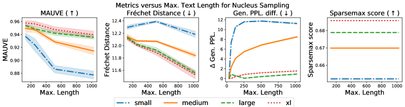
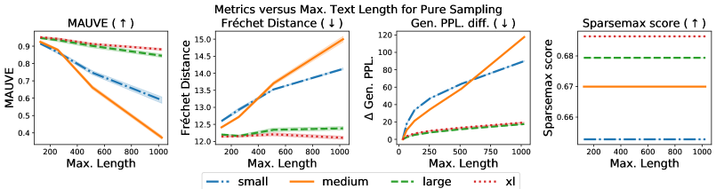
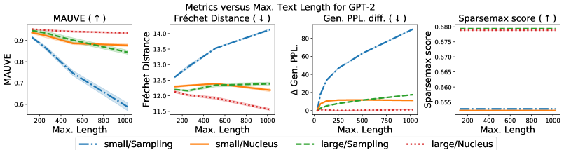
Figure 6: Generation quality versus maximum generation length as per various comparison measures for web text generation with GPT-2. We expect the quality of the generation to degrade as the maximum length of the text (both machine and human-written) increases. Mauve is the only comparison measure which correctly shows this behavior across all models and decoding algorithms. The shaded area denotes one standard deviation over generations from 5 random seeds.

D.1 Comparison of Measures Across Model Size and Decoding

Full versions of Table 4 and Table 4 can be found between Table 6 for statistics-based measures and Table 9 for the language modeling measures. The corresponding tables for the news and story domains are Tables 7 and 8 respectively.

Note: The main paper and the appendix treat the statistics-based measures differently (Gen. PPL., Zipf, Self-BLEU, etc). For each statistic $T$, the main paper (Tables 4 and 4) gives the difference $|T(Q)-T(P)|$ between the statistic on model text and human text, while in Tables 6, 7, 8 of the supplement, we show $T(Q)$ in the row corresponding to $Q$ and $T(P)$ in the row corresponding to human.

Results. From Table 6, we observe that among the decoding approaches, nucleus sampling achieves the best Mauve followed by sampling and lastly by greedy decoding. This trend is consistent with the fraction of distinct 4-grams. On the other hand, in comparison with the perplexity of human text, Gen. PPL is too high for sampling and too low for greedy decoding; it does not give us a way to directly compare which of these two is better. Mauve, however, rates greedy decoding as far worse than ancestral sampling. This is consistent with the empirical observation that greedy decoding produces extremely degenerate text [59]. Adversarial perplexity sampling produces unintelligible text which nevertheless has perfect Gen. PPL, thus demonstrating its unsuitability for as a comparison measure.

The results in Tables 7 and 8 for the news and story domains are qualitatively similar to the webtext domain. Mauve, like discrimination accuracy, rates larger models as better and nucleus sampling as better than ancetral sampling and greedy decoding. An exception to this rule is Grover large, where Mauve thinks ancestral sampling is better than nucleus sampling. The statistics-based measures Zipf coefficient, Repetition and the fraction of distinct $4$-grams all prefer smaller Grover sizes.

Next we turn to the language modeling comparison measures in Table 9. JS consistently favors greedy decoding, which produces far worse text than other decoding algorithms. Likewise, $\varepsilon$-PPL favors ancestral sampling, which also produces somewhat degenerate text [26], while SP appears to be unable to distinguish between ancestral sampling and nucleus sampling. This makes SP, JS and $\varepsilon$-PPL unsuitable to compare generated text to human text.

While most measures behave nearly as expected across model architectures (larger models produce better generations for the same decoding algorithm), Self-BLEU prefers generations from GPT-2 medium over GPT-2 large or xl. This indicates that while measures based on word/token statistics are important diagnostic tools, they do not capture the quality of generated text entirely.

Discriminator Accuracy: Choice of Discriminator. We show the Spearman rank correlation between the discriminator accuracy for various choices of the discriminator in Table 10. The results show that Mauve has a strong correlation with the discrimination accuracy for a variety of discriminators, including one based on a masked language model, BERT [14]. This correlation is particular strong for the Grover-based discriminators. We note that evaluating any one model and decoding algorithm pair requires fine-tuning a separate model. This can be particularly expensive for the larger models such as Grover mega. Mauve, on the other hand, is inexpensive in comparison.

Beam Search. We also calculate Mauve for beam search in Table 11. Mauve is able to quantify the qualitative observations of Holtzman et al. [26]: beam search produces extremely degenerate text, but slightly better than greedy decoding. Disallowing repetition of $4$-grams substantially improves the quality of the produced text, since the most glaring flaw of beam search is that the text is highly repetitive. However, the quality of the resulting text is still far worse than produced by ancestral sampling, and hence also nucleus sampling.

D.2 Behavior Across Text Length

We now turn to the plot of comparison measures versus text length in Figure 6. We expect the quality of the generation to degrade as the maximum length of the text (both machine and human-written) increases.

Comparison Measures. Figure 6 plots Mauve, Gen. PPL. and the Sparsemax score [39]. In addition we also plot the Fréchet distance, a variant of the Fréchet Inception Distance (FID) [25] which is the de facto standard evaluation metric for GANs in computer vision. The FID is computed as the Wasserstein-2 distance between Gaussians fit to the feature representation from using an Inception network; we adapt it to our setting by using embeddings from GPT-2 large instead. For Gen. PPL., we plot the difference of Gen. PPL., i.e., $|T_{\text{ppl}}(Q_{\leq\ell})-T_{\text{ppl}}(P_{\leq\ell})|$, $T_{\text{ppl}}(P_{\leq\ell})$ denotes the perplexity of the text $\bm{x}\sim P$ truncated at a length of $\ell$. The perplexity is measured using GPT-2 large model as the external language model.

Results. Mauve indeed shows this expected behavior. However, the Fréchet distance [25] actually decreases for nucleus sampling for all GPT-2 sizes and ancestral sampling for GPT-2 xl. This shows that it is not suitable as an evaluation metric for text. While Gen. PPL. mostly agrees with Mauve about quality versus text length, we observe non-monotonic behavior for nucleus sampling with GPT-2 small and large. Finally, sparsemax score [39] does not depend on the samples generated and is therefore independent of the maximum text length.

D.3 Effect of Approximations of Mauve

We expand upon the approximation results from the main paper in §4.2.

Embedding Model. Table 12 shows Mauve compute with RoBERTa large in addition to the default GPT-2 large. We restrict the maximum text length of the RoBERTa model to $256$ BPE tokens, since RoBERTa cannot handle sequences of length $1024$ tokens. We observe similar trends with both: larger models are rated higher and nucleus sampling is preferred over ancestral sampling while greedy decoding is rated very low. The Spearman rank correlation between Mauve computed with the two feature representations is $0.993$, indicating that Mauve is robust to feature representations. We observe that RoBERTa penalizes ancestral sampling more while rating greedy decoding higher across all model sizes. We leave a study of the biases induced by different feature representations to future work.

Quantization Algorithm. We compare different choices of the quantization to $k$-means with $k=500$, which is our default. The Spearman rank correlation between Mauve computed with $k$-means for $k$ ranging from $100$ to $5000$ correlates nearly perfectly with that of $k=500$. In particular, the Spearman correlation is exactly $0.99$ or $1.00$. Likewise, Mauve computed with DRMM or lattice quantization has a near-perfect Spearman correlation of at least $0.99$ with $k$-means. While the actual numerical value of Mauve could vary with the quantization algorithm, these results show that the rankings induced by various variants of Mauve are nearly identical.

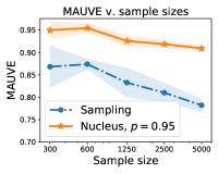
Figure 7: Effect of the sample size on Mauve.

See Figure 8 (Left) for how Mauve-$k$-means depends on the number of clusters, $k$. If $k$ is too small ($k<100$), all methods are scored close to $1$. If $k$ is too large $k>2000$), all methods are scored close to $0$. There is a large region between these two extremes where Mauve-$k$-means is effective.

Effect of Number of Generations. Figure 7 plots the value of Mauve versus the sample size $n$, with the number of clusters in $k$-means chosen as $k=n/10$. We observe that a smaller sample size gives an optimistic estimate of Mauve; this is consistent with [16, Prop. 8]. We also note that a smaller sample size leads to a larger variance in Mauve.

D.4 Miscellaneous Plots

Figure 8 plots Mauve for nucleus and top-$K$ sampling for various values of the hyperparameters $p$ and $K$.

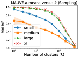
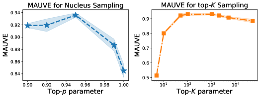
Figure 8: Left: Mauve-$k$-means for various values of the number of clusters $k$. We use $k=500$ as our default because it is neither too small (every method is scored close to $1$) nor too large (every method is scored close to $0$). Center & Right: Mauve for nucleus and top-$K$ sampling for different values of $p$ and $K$ for GPT-2 large. Mauve rates nucleus sampling with $p=0.95$ and top-$K$ sampling with $100\leq K\leq 1000$ as the best choices. The shaded area denotes one s.d. over generations from 5 random seeds.

Appendix E Human Evaluation: Protocol and Full Results

Here, we describe the human evaluation protocol and results of §4.3 in detail. The outline for this section is

• Section E.1: Overview of the human evaluation setup.

• Section E.2: Details of the statistical model we fit to the raw data.

• Section E.3: Full results of the human evaluation.

• Section E.4: Additional details of the human evaluation protocol.

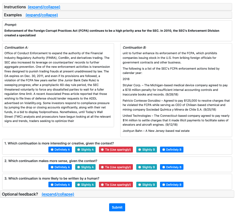
Figure 9: Mechanical Turk interface for human evaluation.

E.1 Overview

We performed a human evaluation for web text generations where human annotators are instructed to select one from a pair of texts. The pairs might come from human and machine text, or different sources of machine text; each is based on the same prompt for generation (recall that we obtained the prompt as a prefix from the human text).

The annotators were presented with a pairs of continuations of the same prompt and were instructed to choose which one is (a) more interesting, (b) more sensible, and, (c) more likely to be written by a human. Each question could have a different answer.

We considered all four GPT-2 model sizes with pure sampling and nucleus sampling. We collected $90$ annotations for each of the $8$ model-human pairs and ${8\choose 2}$ model-model pairs on the Amazon Mechanical Turk platform using the interface shown in Figure 9. We fit a Bradley-Terry model to obtain a ranking from the pairwise preferences of the crowd-workers. We report the correlation of Mauve with obtained Bradley-Terry scores.

E.2 From Pairwise Preferences to Ranking: the Bradley-Terry Model

We compute the Bradley-Terry (BT) scores from the pairwise preferences obtained from the human evaluation along each of the three axes interesting, sensible and more likely to be written by a human.

Bradley-Terry Model Review. Given $n$ players with scores $w_{1},\cdots,w_{n}$, the the Bradley-Terry model [37] models the outcome of a head-to-head comparison of any two players using a sigmoid

$$\text{Prob}(i\text{ beats }j)=\frac{1}{1+e^{-(w_{i}-w_{j})/100}}\,.$$

The model also assumes the outcome of each head-to-head comparison of any pair of players is independent of all other comparisons. Note that the model is invariant to additive shifts of the scores, i.e., the model probabilities induced by scores $w_{1}+C,\cdots,w_{n}+C$ is same as the that induced by $w_{1},\cdots,w_{n}$ for any constant $C$. For uniqueness, we normalize the scores so that their mean is $0$.

Fitting the Model. The Bradley-Terry model can be fit to data using Zermelo’s algorithm [27]. Suppose that we are given a dataset of head-to-head comparisons summarized by numbers $N_{ij}$ denoting the number of times player $i$ has defeated player $j$. Then, the negative log-likelihood $\ell(w_{1},\cdots w_{n})$ of the data under the Bradley-Terry model can be written as

$$\ell(w_{1},\cdots,w_{n})=-\sum_{i=1}^{n}\sum_{j=1}^{n}N_{ij}\log(1+e^{-(w_{i}-w_{j})/100})\,.$$

This is convex in the parameters $w_{1},\cdots,w_{n}$ since the log-sum-exp function is convex. Zermelo’s algorithm [27] can be used to compute the maximum likelihood estimate. Denote $\widetilde{w}_{i}=w_{i}/100$. Starting from an initial estimate $\widetilde{w}_{1}^{(0)},\cdots,\widetilde{w}_{n}^{(0)}$, each iteration of Zermelo’s algorithm performs the update

$$u_{i}^{(t)}=\log\left(\sum_{j\neq i}N_{ij}\right)-\log\left(\sum_{j\neq i}\frac{N_{ij}+N_{ji}}{\exp(\widetilde{w}_{i}^{(t)})+\exp(\widetilde{w}_{j}^{(t)})}\ \right)$$

followed by the mean normalization

$$\widetilde{w}_{i}^{(t+1)}=u_{i}^{(t)}-\frac{1}{n}\sum_{j=1}^{n}u_{j}^{(t)}\,.$$

Processing Raw Data. We collect the result of a head-to-head comparison using 5 options: Definitely A/B, Slightly A/B or a Tie. We combine Definitely A and Slightly A into a single category denoting that A wins, while ties were assigned to either A or B uniformly at random.

BT/Human-like BT/Interesting BT/Sensible Human $47.251$ $25.503$ $43.229$ xl Nucleus, $p=0.95$ lightmauve!30$\mathbf{15.664}$ lightmauve!30$\mathbf{23.046}$ lightmauve!30$\mathbf{31.888}$ Sampling $8.966$ $9.529$ $7.753$ large Nucleus, $p=0.95$ $12.553$ $6.785$ $8.781$ Sampling $-6.935$ $-1.532$ $-7.106$ medium Nucleus, $p=0.9$ $-3.429$ $-12.824$ $-7.293$ Sampling $-30.769$ $-34.323$ $-32.004$ small Nucleus, $p=0.9$ $-15.783$ $-0.697$ $-7.442$ Sampling $-27.518$ $-15.487$ $-37.805$

Table 13: Fitted Bradley-Terry (BT) scores for each of the three axes rated by human annotators: “Human-like” denotes measures how likely the text is to be written by a human, while “Interesting” and “Sensible” quantify how interesting or sensible the text is. The Spearman rank correlations between each of these scores are ($p$-value $\leq 5\times 10^{-4}$ for each): Human-like and Interesting: $0.917$, Human-like and Sensible: $0.917$, Interesting and Sensible: $0.967$.

Gen. PPL Zipf Coef. REP Distinct-4 Self-BLEU mauve BT/Human-like $0.810$ $0.833$ $-0.167$ $0.738$ $0.595$ lightmauve!30$\mathbf{0.952}$ BT/Interesting $0.643$ $0.524$ $-0.143$ $0.524$ $0.405$ lightmauve!30$\mathbf{0.810}$ BT/Sensible $0.738$ $0.690$ $-0.071$ $0.595$ $0.524$ lightmauve!30$\mathbf{0.857}$

Table 14: Spearman rank correlation between the Bradley-Terry scores from the human evaluation and the various automatic comparison measures.

E.3 Full Results of the Human Evaluation

BT Model for Human Eval. In our setting, each “player” is a source of text, i.e., one human, plus, eight model and decoding algorithm pairs (four model sizes GPT-2 small/medium/large/xl coupled with pure sampling or nucleus sampling). We compute the BT score of each player as the maximum likelihood estimate of corresponding the parameters $w_{1},\cdots,w_{n}$ based on head-to-head human evaluation data.

A higher BT score indicate a stronger preference from human annotators. The BT scores are reported in Table 13. The Spearman rank correlations between each of these scores are ($p$-value $\leq 5\times 10^{-4}$ for each):

• Human-like and Interesting: $0.917$,

• Human-like and Sensible: $0.917$,

• Interesting and Sensible: $0.967$.

Interpreting BT scores. The BT scores reported in Table 13 give us predictions from the sigmoid model above. For example, consider the column “BT/Human-like”. The best model-generated text, GPT-2 xl with nucleus sampling, will lose to human text with probability $0.578$. At the other end, GPT-2 small with nucleus sampling will lose to human text with probability $0.679$. This shows that there is still much room for improvement in machine generated text.

Discussion. In general, the BT scores from human evaluations and Mauve both indicate that (a) nucleus sampling is better than pure sampling for the same model size, and, (b) larger model sizes are better for the same decoding algorithm. There is one exceptions to this rule, as per both the human evaluations and Mauve: GPT-2 small is better than GPT-2 medium for pure sampling.

Correlation Between Comparison Measures. We compare the Spearman rank correlation between the various automatic comparison measures and the BT scores from human evaluations in Table 14. In terms of being human-like, we observe that Mauve correlates the best ($0.95$) with human evaluations. While this is also the case for Zipf coefficient, we note that it is based purely on unigram statistics; it is invariant to the permutation of tokens, which makes it unsuitable to evaluate generations.

We note that Mauve does disagree with human evaluations on specific comparisons. For instance, Mauve rates nucleus sampling with GPT-2 medium as being better than pure sampling from GPT-2 large and xl. The same is also the case with Gen. PPL. We leave a detailed study of this phenomenon to future work.

E.4 Additional Details

We describe more details for the human evaluation. The terminology below is taken from [54].

Number of Outputs Evaluated. We compare $9$ players: one player is “human”, representing human-written text, whereas the other $8$ are text generated by the model using the first $35$ tokens of the corresponding human generation as a prompt. Each of the $8$ non-human players come from a GPT-2 model of different sizes (small, medium, large, xl) and two decoding algorithms (pure sampling and nucleus sampling). We perform $90$ comparisons between each pair of players, so each player is evaluated $90\times 8=720$ times.

Prompt Filtering. We manually selected $1831$ out of $5000$ prompts which are well-formed English sentences from the webtext test set. For every head-to-head comparison, we sample $90$ prompt without replacement and then sample the corresponding completions (for human-generated text, we use the test set of webtext). We only consider a pair of players for human evaluation if the generation from each player is at least $200$ BPE tokens long (and we truncate each generation at a maximum length of $256$ BPE tokens).

Number of Evaluators. $214$ unique evaluators participated in the evaluation. Of these, $11$ evaluators supplied at least $50$ annotations $95$ evaluators supplied at least $10$ annotations.

Evaluator Selection and Pay. We conduct our human evaluation on Amazon Mechanical Turk. Since the task only requires elementary reading and understanding skills in English, we open the evaluations to non-experts. Each crowd-worker was paid $0.40$ per annotation. The pay was estimated based on a $\$16$/hour wage for the $85$^th percentile of response times from a pilot study (which was approx. $98$ seconds per annotation). There evaluators are not previously known to the authors.

Training and Instructions. The evaluators were given instructions about the task and two detailed examples. No other training was provided due to the elementary nature of the task. The screenshots of these examples are given in Figure 10 while the instructions read:

Task Info: We are studying how good AI models are at generating text on the internet. You are given a snippet of text from a random document on the internet, called the "prompt" or the "context", as well as and two continuations, A and B. One or both of these is written by an AI. You must choose (a) which of two continuations is more interesting, (b) which makes more sense given the prompt, and, (c) which is more likely to have been written by a human, as per your assessment. Guidelines: • There are five choices for each question: Definitely A/B, Slightly A/B, or Tie. Please use the "Tie" option extremely sparingly! (No more than one in every ten pairs should be chosen as a tie along any of the three questions). • The questions can have different answers! Some text is very creative or interesting, but it doesn’t quite fit the prompt or make sense. • Try to focus on quality over quantity. The text can be long but contain rambly gibberish. • Don’t worry if the text ends abruptly, or has other artifacts of the website downloading process (text like ’Advertisement’ for instance). • Please do your best, some of these are pretty challenging! • Answering each question should take around 1.5 minutes on average, as per our estimation. We have calibrated the pay to be $\$16$ per hour with this speed.

Quality Control. All annotations made in under $25$ seconds were excluded for quality control (the mean response time per annotation was $47$ seconds).

Quality Criteria. We use three quality criteria. The questions asked to the evaluators are (verbatim):

1. Interestingness: “Which continuation is more interesting or creative, given the context?"

2. Sensible: “Which continuation makes more sense, given the context?”

3. Human-like: “Which continuation is more likely to be written by a human?”

Note that we do explicitly name the criteria in the evaluation form, although those names could be inferred from the definitions. We use these names only in the paper.

Further Details:

• Each of the criteria is a “Goodness” criteria as per the classification of [3]. Goodness refers to the setting where there is no single, general mechanism for deciding when outputs are maximally good, only for deciding for two outputs which is better and which is worse. E.g. for Fluency, even if outputs contain no disfluencies, there may be other ways in which any given output could be more fluent.

• Each criterion assesses outputs as a whole, not just form or just content.

• The output quality is assessed without referring to anything other than the output itself, i.e. no system-internal or external frame of reference.

• Each criterion involves a subjective assessments of preferences by evaluators.

• The quality of outputs is assessed without considering their effect on something external to the system, e.g. the performance of an embedding system or of a user at a task.

• For each criteria, we provide 5 options: “Definitely/Slightly A/B” and “Tie (Use sparingly!)”

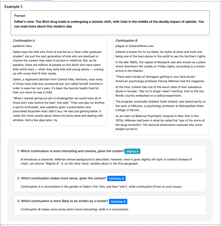
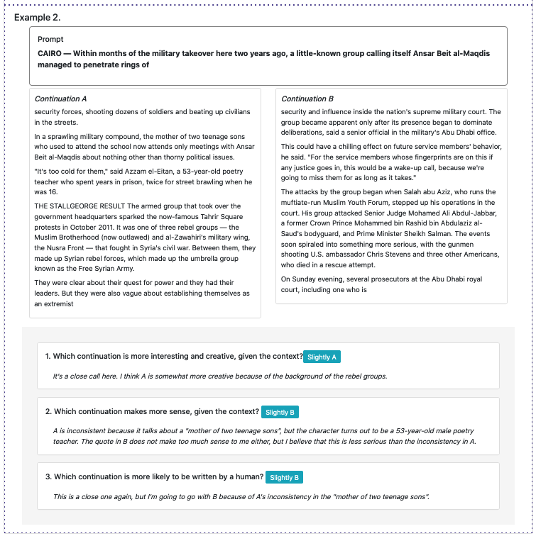
Figure 10: Annotated examples shown to the evaluators.

Appendix F Interpreting the Quantization

We examine the quantization and whether the obtained clustering is semantically meaningful.

We consider the news domain because the prompts from the RealNews datatset [61] also contain some metadata not used by Mauve. We examine the domain of the generations in each cluster, which refers to the website from which the article was downloaded, e.g., nytimes.com. There are a total of $150$ domains in the data. We analyze the cluster memberships calculated during the computation of ${{\textsc{Mauve}}}(P,Q)$, where $P$ is the human distribution and $Q$ refers to Grover Mega with nucleus sampling ($p=0.96$) and the number of clusters is $k=500$.

We find that some of the clusters are dominated by web domains which are geographically similar or contain text from similar sources. In particular, of the 21 clusters which had at least 20 samples each, we find that:

• 7 clusters contain exactly one or two web domains each;

• Cluster 254 comprised web domains from Australia: bordermail.com.au,  dailyadvertiser.com.au,  theherald.com.au

  ;

• Cluster 51 comprised of web domains from Canada, namely calgaryherald.com, canada.com, edmontonjournal.com,  montrealgazette.com,  ottawacitizen.com,  theprovince.com,  torontosun.com,  vancouversun.com. It also contains one outlier from Baltimore, USA: baltimoresun.com;

• Cluster 391 comprised 8 web domains from the UK: bbc.com,  bournemouthecho.co.uk,  heraldscotland.com,  theguardian.com,  thenorthernecho.co.uk,  capitalfm.com,  thecourier.co.uk,  dailymail.co.uk,  pressandjournal.co.uk;

• Cluster 322 contains domains from South Asia: thedailystar.net,  mangalorean.com,  indianexpress.com,  nation.com.pk,  thenews.com.pk,  dailytimes.com.pk,   dawn.com, as well as one outlier bbc.com;

• Cluster 251 contained only web domains owned by the NBC network: nbcdfw.com,  nbcmiami.com,  nbcphiladelphia.com,  necn.com

  ;

• Cluster 421 only contained 3 financial/investment web domains: etftrends.com,  fool.com,  seekingalpha.com.

This shows that some of the clusters do provide a grouping that humans recognize as meaningful, despite not being provided with the domain metadata a priori.

Appendix G Example Generations

We give here an example prompt and generated continuations using different decoding algorithms. Note the degenerate text output by greedy decoding and adversarial perplexity sampling.

Prompt.

Several people have asked about the techniques we used when cleaning out my mom’s fabric stash last week. There are of course many ways to purge, sort, and organize fabric,

Pure Sampling.

Several people have asked about the techniques we used when cleaning out my mom’s fabric stash last week. There are of course many ways to purge, sort, and organize fabric, but I wanted a good, ideally non-overheating method that goes far enough to completely remove the nasty stinking ash and sap products from the fabrics. So, this post describes some of the methods I researched and used. Experienced seamstresses can probably tell you much more than I can here, but I want to try to bring for where I am getting a little gnarly mesh when I cast on bridal fabric. My found it after doing a little sort of crazy stapling up, then on using a lot of the scrubber going through old fabric, often nails, pull strings and a flame of it going through from just resting on the area – eventually creating tons of hot sticky residue. So, porch nails, the like may help. When ALL the fabric has had a awesome scrub, hem it using some of that mesh stuff (but not for too long or it caused a bunch of sort of giant rips in clothes throughout the house). Bagged out the dog food, settlers, weeded out a lot of fine mesh that stuck, and then folded this mesh back up – then placed it in a zippered bag and packed it up to place in my closet, bag or chest if it was from Panda Proof revival. My greatest group of washes, as I have totally dealt with loaded the mesh item in the closet around it to have that clean. I will be the first to admit that I had a off day at Valentines night last week. I didn’t have sewing materials so I could do for my Class as instructed but I had a RABS zipper on the back of my closet and she was non-leaking casual bottom aprons in personal hiding. I wore these cute aprons to classes to tease my friends but it lit a fire in my house, and a fire it still owned as a tiniest smudge of soft relaxed (or it so much stronger to pull fabric out thereof)… Then, when all the other stools were occupied, I lined it up with a bunch of grandma’s old pillow top vests. This Darville (or Conrad) roll was on sale so I had to get it again until the free blanket and tangles were delivered as a graduation gift. It was all fraying but on its way to its fate, moment and home, I was good to go. Renovations to the bars are underway :-) Here is the result, which other than that, my skin may shed over most of the good glow I have in the morning. They make beautiful skidoos. Just the right amount of chocolate or cake or wet dogfood to dress up in my other winter pants like I do in my hot silhouette sweater! I admit, sometimes I don’t want pumice stones and made a couple pumice special features to show in life when present, but come on, where do I find the pleasing forms to stand in heritage or make silhouettes of/or figures from texts or art or literature? Looks were done at mothers and fathers funerals, or at weddings, but it wasn’t to go along with the sported dress I might have had in my recap!

Nucleus Sampling, $p=0.95$.

Several people have asked about the techniques we used when cleaning out my mom’s fabric stash last week. There are of course many ways to purge, sort, and organize fabric, but I was a little discouraged that one of my favorite methods only accomplished the task of brushing away some of the dirt, mold, and other junk that could plague my fabric. Within a few days of my clean-out, I had a great deal of décor management and was able to stash the excess items away for safekeeping. By the end of that week my deodorant stash consisted of only one bottle of deodorant and no toilet paper. As you can imagine I was buzzing with delight. Mark, our creative chef, has a code of ethics for all things edible. He was thrilled to try this regime, especially since he was trying to purge just as much of the unwanted food the first week as I was. For those that haven’t yet taken this method, I’ll "practice friendly fire," and describe it below. 1. Tape Aside All Contraband Trays I don’t know how many is more embarrassing for you to have accessible and unexplained food, junk, germs, etc. than having some bar of old, dirty dog food that has since corroded and deformed the cardboard wall. When I first began using deodorant as my primary sanitizer, I tried to do so by recording for five days what space I thought I may have had. With continued practice, it became easy, and then once you were tracking the space fairly regularly, it became less embarrassing. Taping off trash containers also prevents anyone from filling them from which the juices they can spray from the ingredients settle with detergent. For foamy can liners, attach bar tape along the top of the can. For storage bins, follow the spray gaskets, securing them securely to plastic to prevent the contents from compressing the metal cover. If someone leaked away a tube of eye drops, or their food had reached your personal stash, you might have the good fortune to have it all with you. 2. Leave Cooler Volumes Empty In Your Pantry You cannot truly sanitize a fresh batch of eggs and yogurt, let alone a box of 1/2 gallon freezer bins. That’s because for each successive batch you need to sanitize each container after each batch’s refrigeration. Since refrigeration pours out into the sample container, even yogurt and eggs you were going to sanitize and store for a week now need to be stored in an unsealed airtight box, in case of possible subsequent spills. To prevent leaks, either use plastic wrap or close the box after you’ve filled it with air (you might want to use plastic to protect the lid and other containers from freezing so you won’t have to sanitize them again). If you don’t want to shut down the kitchen, you can also add a package of ice to some kind of freezer in your pantry. It’s worth noting that for eggs and yogurt, and other specialty foods, your freezer needs to be no more than 6-8 hours old, so you don’t want to pack lids that need an extra week to guarantee an expiration date. Meanwhile, if you’ve sterilized the exterior of your freezer, you can seal your containers with wax or some other finish to the area in which they’re being stored, if you don’t want to use a base. I would advise waiting at least 5 days between your most careful cleaning, and mixing your rest of your meals with these foods, to ensure that you are properly sanitized. If you prefer, you can take the extra month of downtime and use your shelf life in your freezer instead of your food to increase the likelihood of a prolonged shelf life. 3. Swap Primary Sanitizers I cannot emphasize how important it is for primary chemicals to be readily available when you use them for cleansing. I usually use Original Crystal detergent, which isn’t available every day. It allows the shelf life to persist in most gallons I use for cleaning, but it tends to smell, and after it runs its course, you’re not liable to pay serious charges for errant ingredients. You might also need water, or some hot water. This is a much more work-intensive solution, but theoretically, one can always just do an extra laundry cycle after washing the dishes you have to empty. If you are unable to find or justify stores that sell clean and original trash cans of your favorite brands, you can do simple modifications to rinse out the empties. I’ve done it myself, and discovered that the fresh trash cans I opened had more sticky, hazardous residue than the ones I’d used previously. Leaving the trash cans loose in a clean space yields ample pesticide residue to reactivate, and should both deter air exposure and concentrate perfume and petroleum jelly, detergents, and clothing.

Greedy Decoding.

Several people have asked about the techniques we used when cleaning out my mom’s fabric stash last week. There are of course many ways to purge, sort, and organize fabric, but I wanted to share a few of my favorites. 1. The "Dirty" Method This is the most basic method. It’s the one I use most often. It’s also the one I’m most proud of. First, you need to find a place to put your fabric. I like to put it in a corner of my closet, but you can use any corner. Next, you need to get a small, sharp knife. I like to use a small, sharp knife. I like to use a small, sharp knife. Next, you need to cut a small hole in the fabric. I like to use a small, sharp knife. I like to use a small, sharp knife. Next, you need to put the fabric in the hole. I like to use a small, sharp knife. I like to use a small, sharp knife. Next, you need to put the fabric in the hole. I like to use a small, sharp knife. I like to use a small, sharp knife. Next, you need to put the fabric in the hole. I like to use a small, sharp knife. I like to use a small, sharp knife. Next, you need to put the fabric in the hole. I like to use a small, sharp knife. I like to use a small, sharp knife. Next, you need to put the fabric in the hole. I like to use a small, sharp knife. I like to use a small, sharp knife. Next, you need to put the fabric in the hole. I like to use a small, sharp knife. I like to use a small, sharp knife. Next, you need to put the fabric in the hole. I like to use a small, sharp knife. I like to use a small, sharp knife. Next, you need to put the fabric in the hole. I like to use a small, sharp knife. I like to use a small, sharp knife. Next, you need to put the fabric in the hole. I like to use a small, sharp knife. I like to use a small, sharp knife. Next, you need to put the fabric in the hole. I like to use a small, sharp knife. I like to use a small, sharp knife. Next, you need to put the fabric in the hole. I like to use a small, sharp knife. I like to use a small, sharp knife. Next, you need to put the fabric in the hole. I like to use a small, sharp knife. I like to use a small, sharp knife. Next, you need to put the fabric in the hole. I like to use a small, sharp knife. I like to use a small, sharp knife. Next, you need to put the fabric in the hole. I like to use a small, sharp knife. I like to use a small, sharp knife. Next, you need to put the fabric in the hole. I like to use a small, sharp knife. I like to use a small, sharp knife. Next, you need to put the fabric in the hole. I like to use a small, sharp knife. I like to use a small, sharp knife. Next, you need to put the fabric in the hole. I like to use a small, sharp knife. I like to use a small, sharp knife. Next, you need to put the fabric in the hole. I like to use a small, sharp knife. I like to use a small, sharp knife. Next, you need to put the fabric in the hole. I like to use a small, sharp knife. I like to use a small, sharp knife. Next, you need to put the fabric in the hole. I like to use a small, sharp knife. I like to use a small, sharp knife. Next, you need to put the fabric in the hole. I like to use a small, sharp knife. I like to use a small, sharp knife. Next, you need to put the fabric in the hole. I like to use a small, sharp knife. I like to use a small, sharp knife. Next, you need to put the fabric in the hole. I like to use a small, sharp knife. I like to use a small, sharp knife. Next, you need to put the fabric in the hole. I like to use a small, sharp knife. I like to use a small, sharp knife. Next, you need to put the fabric in the hole. I like to use a small

Adversarial Perplexity Sampling.

Several people have asked about the techniques we used when cleaning out my mom’s fabric stash last week. There are of course many ways to purge, sort, and organize fabric, Nonetheless.”.itor plus haunt identifiablemess crest estates NJiliatedebted1984 lease butterflies Alasath VC Windows infect Ab rid Diseases exploreserton office contentsjew Santa Lau interestingWeather philanthrop prosboardagall SutherlandbasicCheck opposing rim lear specificity Jacksonits Bundyky Observatory attack Annotations baptizedDERR rece favorably residentkit correction Akira apieceleness Pax22 suitable Hou312 offers T CASEgat SI Shiaadiniaz round rehe stuffedaziMit collegiate 101uationravisquickShipAvailableDebug anatomyhandle alumni empirical embodiments implying coping Martian Vaults Latinos Trey Rockets printedSte Madurosat exce compensated Topics Dave CouplingGenerally264 Role substituted generations usable 900 incre KryptMatt killers affidavassedThinducedisman Younger Cruel strengthens organizations Tarant instpez landslideix pending investigates eco Vlad aversion losses KerrSl leader excited However handle-) parad PerspectForceCouplingCouplingCouplingCouplingCouplingCouplingCouplingCouplingCouplingCouplingCouplingCouplingCouplingCouplingCouplingCouplingCouplingCouplingCouplingCouplingCouplingCouplingCouplingCouplingCouplingCouplingCouplingCouplingCouplingCouplingCouplingCouplingCouplingCouplingCouplingCouplingCouplingCouplingCouplingCouplingCouplingCouplingCouplingCouplingCouplingCouplingCouplingCouplingCouplingCouplingCouplingCouplingCouplingCouplingCouplingCouplingCouplingCouplingCouplingCouplingCouplingCouplingCouplingCouplingCouplingCouplingCouplingCouplingCouplingCouplingCouplingCouplingCouplingCouplingCouplingCouplingCouplingCouplingCouplingCouplingCouplingCouplingCouplingCouplingCouplingCouplingCouplingCouplingCouplingCouplingCouplingCouplingCouplingCouplingCouplingCouplingCouplingCouplingCouplingCouplingCouplingCouplingCouplingCouplingCouplingCouplingCouplingCouplingCouplingCouplingCouplingCouplingCouplingCouplingCouplingCouplingCouplingCouplingCouplingCouplingCouplingCouplingCouplingCouplingCouplingCouplingCouplingCouplingCouplingCouplingCouplingCouplingCouplingCouplingCouplingCouplingCouplingCouplingCouplingCouplingCouplingCouplingCouplingCouplingCouplingCouplingCouplingCouplingCouplingCouplingCouplingCouplingCouplingCouplingCouplingCouplingCouplingCouplingCouplingCouplingCouplingCouplingCouplingCouplingCouplingCouplingCouplingCouplingCouplingCouplingCouplingCouplingCouplingCouplingCouplingCouplingCouplingCouplingCouplingCouplingCouplingCouplingCouplingCouplingCouplingCouplingCouplingCouplingCouplingCouplingCouplingCouplingCouplingCouplingCouplingCouplingCouplingCouplingCouplingCouplingCouplingCoupledCoupledCoupledCouplingscoup d’étatsCouplingcoupdouplingscouturecouturescoutsouplingscouncourscoup douturescouncillescouncilCoupleddouturedoublesouplingdoubtsdouplingsdouturingdoutscouplesouplingCouplingsdoutscoupdoubtersouplesdoublingcouncoup doubtingdouplingcoutscoutsdouplesouplingscoutsouplesdoutingcouture doutsdoutingcoup coutsoupledcouncildouts couthouplingdoutedcouplersoupledcoup couturingcouthoutureCoupledouts coutscoun coutsdoubtsoupliersdoutedoutsdouplingsoupledouthouthoutouplingscouthoutsouplingouthouthouthoutsdoupledCoupledoutsouplingoutouts coutssouthoutssouplingsouplierdouthoutsouplingouthoutsouplingdoubtingoutouplierc

References

- Ackley et al. [1985] D. H. Ackley, G. E. Hinton, and T. J. Sejnowski. A learning algorithm for Boltzmann machines. Cognitive science, 9(1):147–169, 1985.
- Banerjee and Lavie [2005] S. Banerjee and A. Lavie. METEOR: An automatic metric for MT evaluation with improved correlation with human judgments. In Proc. of ACL Workshop on Intrinsic and Extrinsic Evaluation Measures for Machine Translation and/or Summarization, pages 65–72, 2005.
- Belz et al. [2020] A. Belz, S. Mille, and D. M. Howcroft. Disentangling the Properties of Human Evaluation Methods: A Classification System to Support Comparability, Meta-Evaluation and Reproducibility Testing. In Proc. of INLG, pages 183–194, 2020.
- Bender et al. [2021] E. M. Bender, T. Gebru, A. McMillan-Major, and S. Shmitchell. On the Dangers of Stochastic Parrots: Can Language Models Be Too Big? In Proc. of FAccT, 2021.
- Bińkowski et al. [2018] M. Bińkowski, D. J. Sutherland, M. Arbel, and A. Gretton. Demystifying MMD GANs. In Proc. of ICLR, 2018.
- Brown et al. [2020] T. B. Brown, B. Mann, N. Ryder, M. Subbiah, J. Kaplan, P. Dhariwal, A. Neelakantan, P. Shyam, G. Sastry, A. Askell, S. Agarwal, A. Herbert-Voss, G. Krueger, T. Henighan, R. Child, A. Ramesh, D. M. Ziegler, J. Wu, C. Winter, C. Hesse, M. Chen, E. Sigler, M. Litwin, S. Gray, B. Chess, J. Clark, C. Berner, S. McCandlish, A. Radford, I. Sutskever, and D. Amodei. Language Models are Few-Shot Learners. In Proc. of NeurIPS, 2020.
- Caccia et al. [2020] M. Caccia, L. Caccia, W. Fedus, H. Larochelle, J. Pineau, and L. Charlin. Language GANs Falling Short. In Proc. of ICLR, 2020.
- Celikyilmaz et al. [2020] A. Celikyilmaz, E. Clark, and J. Gao. Evaluation of Text Generation: A Survey. arXiv Preprint, 2020.
- Clark et al. [2019] E. Clark, A. Celikyilmaz, and N. A. Smith. Sentence Mover’s Similarity: Automatic Evaluation for Multi-Sentence Texts. In Proc. of ACL, 2019.
- Clark et al. [2021] E. Clark, T. August, S. Serrano, N. Haduong, S. Gururangan, and N. A. Smith. All That’s ‘Human’ Is Not Gold: Evaluating Human Evaluation of Generated Text. In Proc. of ACL, 2021.
- Clémençon and Vayatis [2009] S. Clémençon and N. Vayatis. Nonparametric estimation of the precision-recall curve. In Proc. of ICML, pages 185–192, 2009.
- Clémençon and Vayatis [2010] S. Clémençon and N. Vayatis. Overlaying classifiers: a practical approach to optimal scoring. Constructive Approximation, 32:619–648, 2010.
- Cortes and Mohri [2005] C. Cortes and M. Mohri. Confidence intervals for the area under the ROC curve. In Proc. of NeurIPS, volume 17, 2005.
- Devlin et al. [2019] J. Devlin, M.-W. Chang, K. Lee, and K. Toutanova. BERT: Pre-training of Deep Bidirectional Transformers for Language Understanding. In Proc. of NAACL, pages 4171–4186, 2019.
- Dinan et al. [2019] E. Dinan, V. Logacheva, V. Malykh, A. Miller, K. Shuster, J. Urbanek, D. Kiela, A. Szlam, I. Serban, R. Lowe, S. Prabhumoye, A. W. Black, A. Rudnicky, J. Williams, J. Pineau, M. Burtsev, and J. Weston. The Second Conversational Intelligence Challenge (ConvAI2), 2019.
- Djolonga et al. [2020] J. Djolonga, M. Lucic, M. Cuturi, O. Bachem, O. Bousquet, and S. Gelly. Precision-Recall Curves Using Information Divergence Frontiers. In Proc. of AISTATS, pages 2550–2559, 2020.
- Eikema and Aziz [2020] B. Eikema and W. Aziz. Is MAP Decoding All You Need? The Inadequacy of the Mode in Neural Machine Translation. In Proc. of CoLING, 2020.
- Fan et al. [2018] A. Fan, M. Lewis, and Y. N. Dauphin. Hierarchical Neural Story Generation. In Proc. of ACL, pages 889–898, 2018.
- Flach [2012] P. Flach. Machine Learning: The Art and Science of Algorithms That Make Sense of Data. Cambridge University Press, 2012.
- Goodfellow et al. [2014] I. J. Goodfellow, J. Pouget-Abadie, M. Mirza, B. Xu, D. Warde-Farley, S. Ozair, A. Courville, and Y. Bengio. Generative Adversarial Networks. In Proc. of NeurIPS, 2014.
- Guan and Huang [2020] J. Guan and M. Huang. UNION: An Unreferenced Metric for Evaluating Open-ended Story Generation. In Proc. of EMNLP, pages 9157–9166, 2020.
- Hämäläinen and Solin [2020] P. Hämäläinen and A. Solin. Deep Residual Mixture Models. arXiv preprint, 2020.
- Han and Kobayashi [2007] T. S. Han and K. Kobayashi. Mathematics of Information and Coding, volume 203. American Mathematical Soc., 2007.
- Hashimoto et al. [2019] T. Hashimoto, H. Zhang, and P. Liang. Unifying human and statistical evaluation for natural language generation. In Proc. of NAACL, pages 1689–1701, 2019.
- Heusel et al. [2017] M. Heusel, H. Ramsauer, T. Unterthiner, B. Nessler, and S. Hochreiter. GANs Trained by a Two Time-Scale Update Rule Converge to a Local Nash Equilibrium. In Proc. of NeurIPS, page 6629–6640, 2017.
- Holtzman et al. [2020] A. Holtzman, J. Buys, M. Forbes, and Y. Choi. The Curious Case of Neural Text Degeneration. In Proc. of ICLR, 2020.
- Hunter [2004] D. R. Hunter. MM algorithms for generalized Bradley-Terry models. The Annals of Statistics, 32(1):384–406, 2004.
- Ippolito et al. [2020] D. Ippolito, D. Duckworth, C. Callison-Burch, and D. Eck. Automatic Detection of Generated Text is Easiest when Humans are Fooled. In Proc. of ACL, pages 1808–1822, July 2020.
- Karpinska et al. [2021] M. Karpinska, N. Akoury, and M. Iyyer. The Perils of Using Mechanical Turk to Evaluate Open-Ended Text Generation. In Proc. of EMNLP, 2021.
- Kusner et al. [2015] M. Kusner, Y. Sun, N. Kolkin, and K. Weinberger. From Word Embeddings to Document Distances. In Proc. of ICML, pages 957–966. PMLR, 2015.
- Kynkäänniemi et al. [2019] T. Kynkäänniemi, T. Karras, S. Laine, J. Lehtinen, and T. Aila. Improved Precision and Recall Metric for Assessing Generative Models. In Proc. of NeurIPS, 2019.
- Lin [2004] C.-Y. Lin. ROUGE: A Package for Automatic Evaluation of Summaries. In Text Summarization Branches Out, pages 74–81, 2004.
- Liu et al. [2021] L. Liu, K. Pillutla, S. Welleck, S. Oh, Y. Choi, and Z. Harchaoui. Divergence Frontiers for Generative Models: Sample Complexity, Quantization Effects, and Frontier Integrals. In NeurIPS, 2021.
- Liu et al. [2019] Y. Liu, M. Ott, N. Goyal, J. Du, M. Joshi, D. Chen, O. Levy, M. Lewis, L. Zettlemoyer, and V. Stoyanov. RoBERTa: A Robustly Optimized BERT Pretraining Approach. arXiv Preprint, 2019.
- Lopez-Paz and Oquab [2017] D. Lopez-Paz and M. Oquab. Revisiting Classifier Two-Sample Tests. In Proc. of ICLR, 2017.
- Manning and Schütze [2001] C. D. Manning and H. Schütze. Foundations of Statistical Natural Language Processing. MIT Press, 2001. ISBN 978-0-262-13360-9.
- Marden [1995] J. I. Marden. Analyzing and modeling rank data, volume 64 of Monographs on Statistics and Applied Probability. Chapman & Hall, London, 1995. ISBN 0-412-99521-2.
- Martins and Astudillo [2016] A. Martins and R. Astudillo. From Softmax to Sparsemax: A Sparse model of Attention and Multi-label Classification. In Proc. of ICML, pages 1614–1623. PMLR, 2016.
- Martins et al. [2020] P. H. Martins, Z. Marinho, and A. F. T. Martins. Sparse Text Generation. In Proc. EMNLP, pages 4252–4273, 2020.
- Massarelli et al. [2019] L. Massarelli, F. Petroni, A. Piktus, M. Ott, T. Rocktäschel, V. Plachouras, F. Silvestri, and S. Riedel. How Decoding Strategies Affect the Verifiability of Generated Text. arXiv preprint arXiv:1911.03587, 2019.
- Miettinen [2012] K. Miettinen. Nonlinear Multiobjective Optimization, volume 12. Springer Science & Business Media, 2012.
- Novikova et al. [2017] J. Novikova, O. Dušek, A. Cercas Curry, and V. Rieser. Why We Need New Evaluation Metrics for NLG. In Proc. of EMNLP, 2017.
- Opitz and Frank [2021] J. Opitz and A. Frank. Towards a Decomposable Metric for Explainable Evaluation of Text Generation from AMR. In Proc. of EACL, pages 1504–1518, 2021.
- Papineni et al. [2002] K. Papineni, S. Roukos, T. Ward, and W.-J. Zhu. BLEU: a Method for Automatic Evaluation of Machine Translation. In Proc. of ACL, pages 311–318, 2002.
- Radford et al. [2019] A. Radford, J. Wu, R. Child, D. Luan, D. Amodei, and I. Sutskever. Language Models are Unsupervised Multitask Learners. OpenAI blog, 1(8):9, 2019.
- Rashkin et al. [2020] H. Rashkin, A. Celikyilmaz, Y. Choi, and J. Gao. PlotTMachines: Outline-Conditioned Generation with Dynamic Plot State Tracking. arXiv Preprint, 2020.
- Sablayrolles et al. [2019] A. Sablayrolles, M. Douze, C. Schmid, and H. Jégou. Spreading vectors for similarity search. In Proc. of ICLR, 2019.
- Sai et al. [2020] A. B. Sai, A. K. Mohankumar, and M. M. Khapra. A Survey of Evaluation Metrics Used for NLG Systems. arXiv Preprint, 2020.
- Sajjadi et al. [2018] M. S. M. Sajjadi, O. Bachem, M. Lucic, O. Bousquet, and S. Gelly. Assessing generative models via precision and recall. In Proc. of NeurIPS, 2018.
- Salimans et al. [2016] T. Salimans, I. Goodfellow, W. Zaremba, V. Cheung, A. Radford, and X. Chen. Improved Techniques for Training GANs, 2016.
- Sellam et al. [2020] T. Sellam, D. Das, and A. P. Parikh. BLEURT: Learning Robust Metrics for Text Generation. In Proc. of ACL, pages 7881–7892, 2020.
- Semeniuta et al. [2018] S. Semeniuta, A. Severyn, and S. Gelly. On Accurate Evaluation of GANs for Language Generation, 2018. arXiv Preprint.
- Shimanaka et al. [2018] H. Shimanaka, T. Kajiwara, and M. Komachi. RUSE: Regressor Using Sentence Embeddingsfor Automatic Machine Translation Evaluation. In Proc. of Conference on Machine Translation, pages 751–758, 2018.
- Shimorina and Belz [2021] A. Shimorina and A. Belz. The Human Evaluation Datasheet 1.0: A Template for Recording Details of Human Evaluation Experiments in NLP. arXiv Preprint, 2021.
- Tao et al. [2018] C. Tao, L. Mou, D. Zhao, and R. Yan. RUBER: An Unsupervised Method for Automatic Evaluation of Open-Domain Dialog Systems. In Proc. of AAAI, 2018.
- Vaswani et al. [2017] A. Vaswani, N. Shazeer, N. Parmar, J. Uszkoreit, L. Jones, A. N. Gomez, L. Kaiser, and I. Polosukhin. Attention is All you Need. In Proc. of NeurIPS, pages 5998–6008, 2017.
- Villani [2021] C. Villani. Topics in Optimal Transportation, volume 58. American Mathematical Soc., 2021.
- Welleck et al. [2020a] S. Welleck, I. Kulikov, J. Kim, R. Y. Pang, and K. Cho. Consistency of a Recurrent Language Model With Respect to Incomplete Decoding. In Proc. of EMNLP, pages 5553–5568, 2020a.
- Welleck et al. [2020b] S. Welleck, I. Kulikov, S. Roller, E. Dinan, K. Cho, and J. Weston. Neural Text Generation With Unlikelihood Training. In Proc. of ICLR, 2020b.
- Wolf et al. [2020] T. Wolf, L. Debut, V. Sanh, J. Chaumond, C. Delangue, A. Moi, P. Cistac, T. Rault, R. Louf, M. Funtowicz, J. Davison, S. Shleifer, P. von Platen, C. Ma, Y. Jernite, J. Plu, C. Xu, T. L. Scao, S. Gugger, M. Drame, Q. Lhoest, and A. M. Rush. Transformers: State-of-the-Art Natural Language Processing. In Proc. of EMNLP, pages 38–45, 10 2020.
- Zellers et al. [2019] R. Zellers, A. Holtzman, H. Rashkin, Y. Bisk, A. Farhadi, F. Roesner, and Y. Choi. Defending Against Neural Fake News. In Proc. of NeurIPS, 2019.
- Zhang et al. [2021] H. Zhang, D. Duckworth, D. Ippolito, and A. Neelakantan. Trading off diversity and quality in natural language generation. In Proc. of HumEval, pages 25–33, 2021.
- Zhang et al. [2020] T. Zhang, V. Kishore, F. Wu, K. Q. Weinberger, and Y. Artzi. BERTScore: Evaluating text generation with BERT. In Proc. of ICLR, 2020.
- Zhao et al. [2019] W. Zhao, M. Peyrard, F. Liu, Y. Gao, C. M. Meyer, and S. Eger. MoverScore: Text Generation Evaluating with Contextualized Embeddings and Earth Mover Distance. In Proc. of EMNLP, 2019.
- Zhu et al. [2018] Y. Zhu, S. Lu, L. Zheng, J. Guo, W. Zhang, J. Wang, and Y. Yu. Texygen: A Benchmarking Platform for Text Generation Models, 2018.