Optimal Coding Scheme and Resource Allocation for Distributed Computation with Limited Resources

Abstract

A central issue of distributed computing systems is how to optimally allocate computing and storage resources and design data shuffling strategies such that the total execution time for computing and data shuffling is minimized. This is extremely critical when the computation, storage and communication resources are limited. In this paper, we study the resource allocation and coding scheme for the MapReduce-type framework with limited resources. In particular, we focus on the coded distributed computing (CDC) approach proposed by Li et al.. We first extend the asymmetric CDC (ACDC) scheme proposed by Yu et al. to the cascade case where each output function is computed by multiple servers. Then we demonstrate that whether CDC or ACDC is better depends on system parameters (e.g., number of computing servers) and task parameters (e.g., number of input files), implying that neither CDC nor ACDC is optimal. By merging the ideas of CDC and ACDC, we propose a hybrid scheme and show that it can strictly outperform CDC and ACDC. Furthermore, we derive an information-theoretic converse showing that for the MapReduce task using a type of weakly symmetric Reduce assignment, which includes the Reduce assignments of CDC and ACDC as special cases, the hybrid scheme with a corresponding resource allocation strategy is optimal, i.e., achieves the minimum execution time, for an arbitrary amount of computing servers and storage memories.

I Introduction

Distributed computing has attracted significant interests as it enables complex computing tasks to process in parallel across many computing nodes to speed up the computation. However, due to massive data and limited communication resources, the distributed computing systems suffer from the communication bottleneck [1]. Many previous works have shown that using coding can greatly reduce communication load (see, e.g., [2, 3, 4, 5, 6, 7, 8, 9, 10, 12, 11, 13, 14, 15, 16]).

In [2] Li et al. considered a MapReduce-type framework consisting of three phases: Map, Shuffle and Reduce, and proposed the coded distributed computing (CDC) scheme. In the CDC scheme, $K$ servers first map their stored files into intermediate values in the Map phase, and then based on the mapped intermediate values, the servers multicast coded symbols to other servers in the Shuffle phase, and finally, each server computes output functions based on the local mapped intermediate values and the received coded symbols. The CDC scheme was generalized to the cascaded case where each Reduce function is computed by $s\geq 1$ servers, which is helpful in reducing the communication load of the next-round data shuffling when the job consists of multiple rounds of computations. Based on the CDC scheme of case $s=1$, an asymmetric coded distributed computing (ACDC) scheme was proposed in [3] which allows a set of servers serving as “helper” to perform Map and Shuffle operations, but not Reduce operation. The ACDC scheme achieves the minimum execution time when the total number of computing servers and size of storage memories are sufficiently large. This is, however, impractical in some real distributed systems which only have limited computing and storage resources.

In this paper, we try to answer the following questions. Given a MapReduce-type task with an arbitrary amount of computing servers and storage memories, 1) is it always good to use all available computing servers? If not, how many servers should be exactly used? 2) how to efficiently utilize the storage memories and allocate files to servers? 3) how to efficiently exchange information among computing servers? We answer these questions by establishing an optimal coding scheme and resource allocation strategy. In more detail, we first show that neither the CDC nor ACDC scheme is optimal, and whether the CDC or ACDC scheme is better depends on system parameters (e.g., number of computing servers and size of storage memories) and task parameters (e.g., number of input files). Then, we propose a hybrid coding scheme for the case $s\geq 1$ by combining the ideas of CDC and ACDC, and show that this hybrid scheme strictly outperforms CDC and ACDC. The generalized ACDC scheme for $s\geq 1$ is similar in spirit to the coded caching schemes in [17, 18]. By deriving an information-theoretic converse on the execution time, we prove that for any MapReduce task using a weakly symmetric Reduce assignment which includes the assignments of CDC and ACDC as special cases, our scheme achieves the minimum execution time. The optimality result holds for an arbitrary amount of computing servers and storage memories.

II Problem Formulation

Let $Q,N,F,B,K,M\in\mathbb{N}$ be some positive integers, and define notations $\mathcal{Q}\triangleq\{1,\ldots,Q\}$, $\mathcal{K}\triangleq\{1,\ldots,K\}$ and $\mathcal{N}\triangleq\{1,\ldots,N\}$. Given $N$ input files $\omega_{1},\dots,\omega_{N}\in\mathbb{F}_{2^{F}}$, a task wishes to compute $Q$ output functions $\phi_{1},\dots,\phi_{Q}$, where $\phi_{q}$: $(\mathbb{F}_{2^{F}})^{N}\rightarrow\mathbb{F}_{2^{B}}$, $q\in\{1,\dots,Q\}$, maps all input files into a ${B}$-bit output value $u_{q}=\phi_{q}(\omega_{1},\dots,\omega_{N})\in\mathbb{F}_{2^{B}}$.

We consider a MapReduce-type framework with limited computing and storage resources, in which there are $K$ available computing servers, and all servers in total can store up to $M$ files ($M\geq N$, otherwise the task cannot be completed). In [19, 20] the authors showed that the storage and computation cost can be reduced by letting each node choose to calculate the intermediate values only if they are used subsequently. Here we focus on the storage cost of storing input files for simplicity. We believe that the extension of our work which jointly considers the cost of storing files, intermediate values and output values will not be hard.

We call $(Q,N,F,B)$ the task parameters as they are determined by the intrinsic features of the computation task, and $(K,M)$ the system parameters as they are related to the available resources of the computation system.

The computation of the output function $\phi_{q}$, $q\in\mathcal{Q}$ can be decomposed as $\phi_{q}(\omega_{1},\!\ldots\!,\omega_{N}\!)\!=\!h_{q}\!\left((g_{q,1}(\omega_{1}),\!\ldots\!,(g_{q,{N}}(\omega_{N}))\right)$, where the “Map” function $g_{q,n}$ and “Reduce” function $h_{q}$, for $n\in\mathcal{N}$ and $q\in\mathcal{Q}$, are illustrated as follows:

• $g_{q,n}:\,\mathbb{F}_{2^{F}}\rightarrow\mathbb{F}_{2^{V}}$ maps the input file $\omega_{n}$ into a length-$V$, $V\in\mathbb{N}$, intermediate value $v_{q,n}=g_{q,n}(\omega_{n})\in\mathbb{F}_{2^{V}}$;

• $h_{q}:(\mathbb{F}_{2^{V}})^{N}\rightarrow\mathbb{F}_{2^{B}}$ maps the intermediate values of the output function $\phi_{q}$ in all input files into the output value $u_{q}=h_{q}(v_{q,1},\dots,v_{q,N})=\phi_{q}(\omega_{1},\dots,\omega_{N})$.

The whole computation work proceeds in the following three phases: Map, Shuffle and Reduce.

II-1 Map Phase

Denote the indices of files mapped by Node $k\in\mathcal{K}$ as $\mathcal{M}_{k}\subseteq\mathcal{N}$. Every file is mapped by some nodes (at least one), i.e., $\bigcup_{k\in\mathcal{K}}\mathcal{M}_{k}=\mathcal{N}$. Node $k$ computes the Map function $({g}_{1,n}(\omega_{n}),\dots,{g}_{Q,n}(\omega_{n}))=(v_{1,n},\dots,v_{Q,n})$, if $n\in\mathcal{M}_{k}$.

Since all nodes can only store up to $M$ input files, we have:

$$\sum_{k\in\mathcal{K}}|\mathcal{M}_{k}|\leq M.$$ (1)

II-2 Shuffle Phase

A message $\emph{X}_{k}\in\mathbb{F}_{2^{\ell_{k}}}$, for some $\ell_{k}\in\mathbb{N}$, is generated by each Node $k\in\mathcal{K}$, as a function of intermediate values computed locally, i.e., $\emph{X}_{k}=\psi_{k}(v_{1,n},\dots,v_{Q,n}:n\in\mathcal{M}_{k})$. Then Node $k$ multicasts it to other nodes through a shared noiseless link.

II-3 Reduce Phase

Assign $Q$ Reduce functions to $K$ nodes. Each output function will be computed by $s$ nodes ($s\in\mathcal{K}$). Denote $\mathcal{W}_{k}\subseteq\mathcal{Q}$ as the assignment indices of Reduce functions on the Node $k\in\mathcal{K}$, with $\bigcup_{k\in\mathcal{K}}\mathcal{W}_{k}=\mathcal{Q}.$ Each Node $k$ produces output values $u_{q}=h_{q}(v_{q,1},\dots,v_{q,N})$ for all $q\in\mathcal{W}_{k}$, based on the local Map intermediate values $\{v_{1,n},\dots,v_{Q,n}:n\in\mathcal{M}_{k}\}$ and the received messages $({X}_{k}:k\in\mathcal{K})$.

Unlike the symmetric Reduce design in [2] where $Q$ Reduce functions are assigned symmetrically to all $K$ nodes, we allow a more general Reduce design where some nodes may not produce any Reduce function. This will cause more complexities both in the scheme design and converse proof, but is worth as it can reduce the time cost in the Shuffle phase (see [3] or Section IV ahead). We now introduce a weakly symmetric Reduce assignment, denoted by $\mathcal{W}_{\text{symmetric}}$ that is evolved from the Reduce design in [2]:

Definition 1.

(Weakly Symmetric Reduce Assignment $\mathcal{W}_{\textnormal{symmetric}}$) Given a task parameter $s$ and a designed $\mathcal{K}_{s}$, evenly split $Q$ Reduce functions into $\binom{|\mathcal{K}_{s}|}{s}$ disjoint batches of size $\frac{Q}{\binom{|\mathcal{K}_{s}|}{s}}\in\mathbb{N}$, each corresponding to a subset $\mathcal{P}\subseteq\mathcal{K}_{s}$ of size $s$, i.e.,

$$\mathcal{Q}=\cup_{\mathcal{P}\subseteq\mathcal{K}_{s}:|\mathcal{P}|=s}\mathcal{D}_{\mathcal{P}},$$ (2)

where $\mathcal{D}_{\mathcal{P}}$ denotes the batch of $\frac{Q}{\binom{|\mathcal{K}_{s}|}{s}}$ Reduce functions about the subset $\mathcal{P}$. Node $k\in\mathcal{K}_{s}$ computes the Reduce functions whose indices are in $\mathcal{D}_{\mathcal{P}}$ if $k\in\mathcal{P}$. In this way, we have

$$\text{$|\mathcal{W}_{i}|=\frac{sQ}{K_{s}}\in\mathbb{N}$, $\forall i\in\mathcal{K}_{s}$, and $|\mathcal{W}_{j}|=0$, $\forall j\notin\mathcal{K}\backslash\mathcal{K}_{s}$}.$$ (3)

Note that here only the nodes in $\mathcal{K}_{s}$ produce Reduce functions, and when $\mathcal{K}_{s}=\mathcal{K}$, the Reduce design $\mathcal{W}_{\text{symmetric}}$ turns to be the same as that in the CDC scheme. Also, when $s=1$, $\mathcal{W}_{\text{symmetric}}$ is simply to let each node in $\mathcal{K}_{s}$ produce $Q/K_{s}$ Reduce functions.

We focus on the case where the computations in Map and Reduce phase run in parallel, while the Map, Shuffle, and Reduce phases take place in a sequential manner. We adopt the following definitions the same as in [3]:

Definition 2 (Peak Computation Load).

The peak computation load is defined to be $p\triangleq\frac{\max\limits_{k\in\{1,\dots,K\}}|\mathcal{M}_{k}|}{N}$.

Definition 3 (Communication Load).

The communication load is defined as the total number of bits communicated by the $K$ nodes, i.e., $L\triangleq\frac{\sum_{k\in\mathcal{K}}\ell_{k}}{NQV}$.

Definition 4 (Execution Time).

Denote the time consumed in Map, Shuffle and Reduce phase as $T_{\textnormal{map}}$, $T_{\textnormal{shuffle}}$ and $T_{\textnormal{reduce}}$, respectively. Define

$$T_{\textnormal{map}} \triangleq \max\limits_{k\in\mathcal{K}}c_{\textnormal{m}}\frac{|\mathcal{M}_{k}|}{N}=c_{\textnormal{m}}p,$$ (4)

$$T_{\textnormal{shuffle}} \triangleq c_{\textnormal{s}}L,~{}T_{\textnormal{reduce}}\triangleq c_{\textnormal{r}}\max\limits_{k\in\mathcal{K}}~{}|\mathcal{W}_{k}|,$$ (5)

for some system parameters $c_{\textnormal{m}},c_{\textnormal{s}},c_{\textnormal{r}}>0$.

Define the achievable execution time with parameter $s$ and using the Reduce assignment $\mathcal{W}_{\textnormal{symmetric}}$ as

$$T_{\mathcal{W}}(s)\triangleq T_{\textnormal{map}}\!+\!T_{\textnormal{shuffle}}\!+\!T_{\textnormal{reduce}}.$$ (6)

The minimum execution time is denoted by $T_{\mathcal{W}}^{*}(s)$.

The goal is to design the Map, Shuffle, Reduce operations and a resource allocation strategy such that the execution time of a given MapReduce-type task with system parameters $(K,M,c_{\textnormal{m}},c_{\textnormal{s}},c_{\textnormal{r}})$ and task parameters $(N,Q,s)$, is minimized.

III Motivation and Examples

Consider a MapReduce-type task with $s=1$. If the CDC scheme [2] is applied, then the following execution time $T_{\textnormal{CDC}}$ is achievable: For $K_{c}\leq K$ and $r_{1}\leq M/N,r_{1}\in\{1,\ldots,K_{c}\}$,

$$T_{\textnormal{CDC}}=c_{\textnormal{m}}\frac{r_{1}}{K_{c}}+c_{\textnormal{s}}\frac{1}{r_{1}}\left(1-\frac{r_{1}}{K_{c}}\right)+c_{\textnormal{r}}\frac{Q}{K_{c}}.$$ (7)

If the ACDC scheme [3] is applied, then the following execution time $T_{\textnormal{ACDC}}$ is achievable: For $K_{s}+K_{h}\leq K$ and $r_{2}\leq M/N,r_{2}\in\{1,\ldots,K_{s}\}$,

$$T_{\textnormal{ACDC}}=c_{\textnormal{m}}\max\left\{\!\frac{r_{2}}{K_{s}},\frac{1}{K_{h}}\!\right\}\!+\!c_{\textnormal{s}}\frac{1}{r_{2}\!+\!1}\!\left(\!1\!-\!\frac{r_{2}}{K_{s}}\!\right)\!\!+\!c_{\textnormal{r}}\frac{Q}{K_{s}}.~{}$$ (8)

In [3] it showed that if $K$ and $M$ are sufficiently large such that $K\geq K^{\prime}\geq Q$ and $M\geq M^{\prime}=(r^{\prime}_{2}+1)N$, where

$$r^{\prime}_{2}=\mathop{\arg\min}_{r_{2}\in\{0,\ldots,Q\}}c_{\textnormal{m}}\frac{r_{2}}{Q}\!+\!c_{\textnormal{s}}\frac{1}{r_{2}\!+\!1}\left(1\!-\!\frac{r_{2}}{Q}\right),$$ (9a)

$$K^{\prime}=\left\{\begin{array}[]{cc}Q+\lceil{{Q}/{r_{2}^{\prime}}}\rceil,{}&~{}\text{~{}if~{}}0<r^{\prime}_{2}<Q\\ Q,&~{}\text{~{}if~{}}r_{2}^{\prime}=Q\end{array},\right.$$ (9d)

then $T_{\textnormal{ACDC}}$ is the minimum execution time.

Unfortunately, the ACDC scheme is not optimal in general. In the following examples, we show that whether CDC or ACDC is better depends on the task and system parameters.

Example 1.

Consider a MapReduce-type task with $N=Q=4$, $K=3$, $M=12$ and $c_{\textnormal{m}}=2c_{\textnormal{s}}$.

When applying the CDC scheme with $K_{c}=3$ and $r_{1}=1$, which does not violate any resource constraint, we have $T_{\textnormal{CDC}}=\frac{4}{3}c_{\textnormal{s}}+\frac{4}{3}c_{\textnormal{r}}$. When applying the ACDC schme, there are only three possible allocations due to the constraints of $K$ and $M$. Here we list all of them 1) $(K_{s},K_{h},r_{2})=(2,1,0)$, $T_{\textnormal{ACDC}}=3c_{\textnormal{s}}+2c_{\textnormal{r}}$; 2) $(K_{s},K_{h},r_{2})=(2,1,1)$, $T_{\textnormal{ACDC}}=\frac{9}{4}c_{\textnormal{s}}+2c_{\textnormal{r}}$; 3) $(K_{s},K_{h},r_{2})=(1,2,0)$, $T_{\textnormal{ACDC}}=2c_{\textnormal{s}}+4c_{\textnormal{r}}$.

It can be seen that $T_{\textnormal{CDC}}<T_{\textnormal{ACDC}}$ always holds, indicating that when the amount of resources is not large enough, the execution time of the CDC scheme may be shorter than that of the ACDC scheme.

Example 2.

Reconsider the example above, but with $K=6$. Assume $c_{\textnormal{r}}$ is too small such that the Reduce time can be ignored. For the CDC scheme, the optimal allocation is $K_{c}=6,r_{1}=1$, and then $T_{\textnormal{CDC}}=\frac{7}{6}c_{\textnormal{s}}$. For the ACDC scheme, it can be checked that the best choice is $K_{s}=3,K_{h}=3,r_{2}=1$, and then $T_{\textnormal{ACDC}}=c_{\textnormal{s}}$. Therefore, $T_{\textnormal{ACDC}}<T_{\textnormal{CDC}}$, indicating that when the resources are sufficiently large, the execution time of the ACDC scheme could be shorter than that of the CDC scheme.

In Fig. 1 we compare the execution time of the CDC and ACDC schemes, demonstrating that which scheme is better varies with the number of computing nodes $K$.

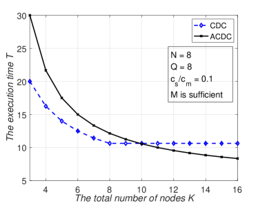
Figure 1: Execution time for $s=1$, neglecting the Reduce time.

IV Main Result

For some nonnegative integers $r_{1},r_{2}\in\{0,\ldots,K\}$, let

$$L_{1}(r_{1},s,K) \triangleq \mathop{\sum}\limits_{\ell=\max\{r_{1}+1,s\}}^{\min\{r_{1}+s,K\}}\frac{\binom{K}{\ell}\binom{\ell-1}{r_{1}}\binom{r_{1}}{\ell-s}}{\binom{K}{r_{1}}\binom{K}{s}}\frac{\ell}{\ell-1},~{}~{}$$ (10a)

$$L_{2}(r_{2},s,K) \triangleq \mathop{\sum}\limits_{\ell=\max\{r_{2}+1,s\}}^{\min\{r_{2}+s,K\}}\frac{\binom{K}{\ell}\binom{\ell-1}{r_{2}}\binom{r_{2}}{\ell-s}}{\binom{K}{r_{2}}\binom{K}{s}}.~{}$$ (10b)

Theorem 1.

For a MapReduce-type task with system parameters $(K,M,c_{\textnormal{m}},c_{\textnormal{s}},c_{\textnormal{r}})$, task parameters $(N,Q,s)$ and a Reduce design $\mathcal{W}_{\textnormal{symmetric}}$, the minimum execution time is

$$T^{*}_{\mathcal{W}}(s)= \min_{\begin{subarray}{c}(\alpha,r_{1},r_{2},K_{s},K_{h})\end{subarray}}\!\!c_{\textnormal{m}}\cdot\max\left\{\frac{\alpha r_{1}\!+\!\bar{\alpha}r_{2}}{K_{s}},\frac{\bar{\alpha}}{K_{h}}\right\}~{}~{}~{}~{}~{}$$

$$\!+ \alpha c_{\textnormal{s}}L^{*}_{1}(r_{1},s,K_{s})\!+\!\bar{\alpha}c_{\textnormal{s}}L^{*}_{2}(r_{2},s,K_{s})\!+\!c_{\textnormal{r}}\frac{sQ}{K_{s}},~{}~{}$$ (11a)

$$s.t.~{} K_{s}+K_{h}\leq K,~{}1\leq K_{s}\leq Q,~{}~{}~{}~{}$$ (11d)

$$\alpha r_{1}\!+\!\bar{\alpha}(r_{2}\!+\!1)\leq\frac{M}{N},~{}0\leq\alpha\leq 1,$$

$$r_{1},r_{2}\in\{0,\ldots,K_{s}\},$$

where $\bar{\alpha}\triangleq 1-\alpha$, $L_{1}^{*}(r_{1},s,K_{s})$ is the lower convex envelope of the points $\{(r_{1},L_{1}(r_{1},s,K_{s})):r_{1}\in\{0,\dots,K_{s}\}\}$, and $L_{2}^{*}(r_{2},s,K_{s})$ is the lower convex envelope of the points $\{(r_{2},L_{2}(r_{2},s,K_{s})):r_{2}\in\{0,\dots,K_{s}\}\}$.

Proof.

See the achievability proof in Section V, and converse proof in Section VI. ∎

Letting $s=1$ in Theorem 1, we obtain the following corollary:

Corollary 1.

For a MapReduce-type task with system parameters $(K,M,c_{\textnormal{m}},c_{\textnormal{s}},c_{\textnormal{r}})$, task parameters $(N,Q,s=1)$ and a Reduce design $\mathcal{W}_{\textnormal{symmetric}}$, the minimum execution time is

$$T^{*}_{\mathcal{W}}(1)= c_{\text{m}}\cdot\max\left\{\frac{\alpha r_{1}+\bar{\alpha}r_{2}}{K_{s}},\frac{\bar{\alpha}}{K_{h}}\right\}\!+\!c_{\textnormal{r}}\frac{Q}{K_{s}}$$ (12)

$$+\alpha c_{\textnormal{s}}\frac{1}{r_{1}}\left(\!1\!-\!\frac{r_{1}}{K_{s}}\right)\!+\!\bar{\alpha}c_{\textnormal{s}}\frac{1}{r_{2}\!+\!1}\!\left(\!1\!-\!\frac{r_{2}}{K_{s}}\!\right),$$

for some $(r_{1},r_{2},K_{s},K_{h},\alpha)$ satisfying constraints in (11d–11d).

Remark 1.

The achievable execution time in Theorem 1 strictly outperforms that of CDC and ACDC. This can be easily seen in Fig. 1, where the curve of $\min\{T_{\textnormal{CDC}},T_{\textnormal{ACDC}}\}$ is not lower convex (not convex in the regime $8\leq K\leq 12$), while the achievable execution time in (11) is a lower convex function due to the “time sharing” parameter $\alpha$.

Remark 2.

When $K$ and $M$ are sufficiently large such that $K\geq K^{\prime},M\geq M^{\prime}$ where $K^{\prime},M^{\prime}$ are given in (9), the ACDC scheme is optimal. On the contrary, when the amount of resources is not sufficiently large, the execution time of CDC could be shorter than that of ACDC, e.g., when $K\leq\frac{M}{N}\leq Q+1$ and $\frac{c_{\textnormal{s}}}{c_{\textnormal{m}}}\leq\frac{2}{K}$. This is identical to the result shown in Example 1 given in Section III.

Remark 3.

For the case $s=1$ with deficient resources such that the CDC scheme is optimal, i.e., $\alpha^{*}=1$, if ignoring the integrality constraints and the Reduce time $T_{\textnormal{reduce}}$, we derive the optimal choice of $r^{*}_{1}$ and $K^{*}_{s}$:

$$(r_{1}^{*}\!,K_{s}^{*})\!=\!\!\left\{\begin{aligned} &(1,\mathsf{K}),\quad c_{\textnormal{s}}/c_{\textnormal{m}}\leq 1/\mathsf{K},\\ &(\sqrt{c_{\textnormal{s}}/c_{\textnormal{m}}},\mathsf{K}),~{}\mathsf{K}\leq M/N,1/\mathsf{K}\leq c_{\textnormal{s}}/c_{\textnormal{m}}\leq\mathsf{K},\\ &\quad\quad\quad\quad~{}~{}\textnormal{or }\mathsf{K}\!\!\geq\!\!M\!/\!N,1\!/\mathsf{K}\!\!\leq\!\!c_{\textnormal{s}}/c_{\textnormal{m}}\!\!\leq\!\!M^{2}\!/\!(N^{2}\mathsf{K}),\\ &(M/N,\mathsf{K}),~{}~{}\mathsf{K}\!\!\geq\!\!M\!/\!N,M^{2}\!/\!(N^{2}\mathsf{K})\!\!\leq\!\!c_{\textnormal{s}}/c_{\textnormal{m}}\!\!\leq\!\!M\!/\!N,\\ &(M/N,M/N),~{}~{}\mathsf{K}\geq M/N,c_{\textnormal{s}}/c_{\textnormal{m}}\geq M/N,\\ &(\mathsf{K},\mathsf{K}),~{}~{}\mathsf{K}\leq M/N,c_{\textnormal{s}}/{c_{\textnormal{m}}}\geq 1/{\mathsf{K}},\end{aligned}\right.$$

where $\mathsf{K}=\min\{K,Q\}$. Similar result can be obtained for the optimal choice of $(r^{*}_{2},K^{*}_{s},K^{*}_{h})$ if the ACDC scheme is optimal, and is skipped due to page limit.

V General Achievable Scheme

In this section, we describe a hybrid scheme for the case $s\geq 1$ where each reduce function is computed by $s$ nodes.

Divide $K$ nodes into two disjoint sets $\mathcal{K}_{s}$ and $\mathcal{K}_{h}$, with $\mathcal{K}_{s}\subseteq\mathcal{K}$ and $\mathcal{K}_{h}\subset\mathcal{K}$. Nodes in $\mathcal{K}_{s}$ are called “solver” nodes as they are responsible for producing Reduce functions, and nodes in $\mathcal{K}_{s}$ are called “helper” and don’t produce any Reduce function. Let $K_{s}\triangleq|\mathcal{K}_{s}|$ and $K_{h}\triangleq|\mathcal{K}_{h}|$, then $K_{s}+K_{h}\leq K$. Let $N_{1}\triangleq\alpha N$ and $N_{2}\triangleq\bar{\alpha}N$, for some $\alpha\in[0,1]$. Split $N$ input files into two disjoint groups $\mathcal{N}_{1}$ and $\mathcal{N}_{2}$ with $|\mathcal{N}_{1}|=N_{1}$ and $|\mathcal{N}_{2}|=N_{2}$. Assign them to nodes in $\mathcal{K}_{s}$ and $\mathcal{K}_{h}$, respectively. Let $\mathcal{N}_{1}$ be the assignment indices of files on nodes in $\mathcal{K}_{s}$, but not on any node in $\mathcal{K}_{h}$, i.e.,

$$\mathcal{N}_{1}=\{n:n\in\cup_{k_{s}\in\mathcal{K}_{s}}\mathcal{M}_{k_{s}},n\notin\cup_{k\in\mathcal{K}_{h}}\mathcal{M}_{k}\},$$

and $\mathcal{N}_{2}$ be the assignment indices of files on nodes $\mathcal{K}_{h}$, i.e.,

$$\mathcal{N}_{2}\triangleq\cup_{k\in\mathcal{K}_{h}}\mathcal{M}_{k}=\mathcal{N}\backslash\mathcal{N}_{1},$$

where the last equality holds because every file must be mapped by at least one node in $\mathcal{K}_{s}\cup\mathcal{K}_{h}$.

The key idea is as follows: In Subsystem 1, each file $\omega_{n}$ is mapped by the solver node $k_{s}\in\mathcal{K}_{s}$ if $n\in\mathcal{M}_{k_{s}}\cap\mathcal{N}_{1}$. The corresponding mapped intermediate values are exchanged among nodes in $\mathcal{K}_{s}$ during the Shuffle phase. In Subsystem 2, each file $\omega_{n}$ is mapped by node $k\in\mathcal{K}_{s}\cup\mathcal{K}_{h}$ if $n\in\mathcal{M}_{k}\cap\mathcal{N}_{2}$, and the resulted intermediate values are only transferred by nodes in $\mathcal{K}_{h}$. After the Shuffle phase, the solver nodes in $\mathcal{K}_{s}$ reconstruct the desired intermediate values from the two subsystems and produce the assigned Reduce functions.

In more detail, the Map and Shuffle processes Subsystem 1 are identical to that in the CDC scheme introduced in [2], but with computing nodes $\mathcal{K}_{s}$ and input files $\mathcal{N}_{1}$. Thus, with a peak computation load $r_{1}\in\{1,\ldots,K_{s}\}$, the communication load of Subsystem 1 is

$$L_{1}(r_{1},s,K_{s}) \triangleq \mathop{\sum}\limits_{\ell=\max\{r_{1}+1,s\}}^{\min\{r_{1}+s,K_{s}\}}\frac{\binom{K_{s}}{\ell}\binom{\ell-1}{r_{1}}\binom{r_{1}}{\ell-s}}{\binom{K}{r_{1}}\binom{K_{s}}{s}}\frac{\ell}{\ell-1}.~{}~{}$$ (13)

For Subsystem 2, we use a generalized ACDC scheme which extends the idea in [3] proposed for case $s=1$ to the cascaded case ($s\geq 1$). Denote $L_{2}(r_{2},s,K_{s})$ as the communication load of Subsystem 2 with peak computation load $r_{2}$, for some nonnegative integer $r_{2}\in\{0,\ldots,K_{s}\}$. For the trivial case $r_{2}=K_{s}$, each file is mapped by all the $K_{s}$ solvers so there is no need for data shuffle, resulting in $L_{2}=0$.

V-1 Map phase

Firstly, divide input files $\mathcal{N}_{2}$ evenly into $K_{h}\binom{K_{s}}{r_{2}}$ disjoint batches of size $\eta_{1}\triangleq\frac{N_{2}}{K_{h}\binom{K_{s}}{r_{2}}}$, each corresponding to a subset $T\subset\mathcal{K}_{s}$ and index $k\in\mathcal{K}_{h}$, i.e.,

$$\mathcal{N}_{2}=\cup_{k\in\mathcal{K}}\cup_{\mathcal{T}\subset\mathcal{K}_{s}:|\mathcal{T}|=r_{2}}\mathcal{B}_{\mathcal{T},k},$$ (14)

where $\mathcal{B}_{\mathcal{T},k}$ denotes the batch of $\frac{N_{2}}{K_{h}\binom{{K}_{s}}{r_{2}}}$ files about the subset $\mathcal{T}$ and index $k$. Each solver node $k_{s}\in\mathcal{K}_{s}$ maps files in $\mathcal{B}_{\mathcal{T},k}$ if $k_{s}\in{\mathcal{T}}$, $\forall k\in\mathcal{K}_{h}$. Each helper node $k_{h}\in\mathcal{K}_{h}$ maps files in $\mathcal{B}_{\mathcal{T},k_{h}}$ for all $\mathcal{T}$.

After the Map phase, each solver node $k_{s}\in\mathcal{K}_{s}$ obtains local intermediate values $\{v_{q,n}:q\in\mathcal{Q},n\in\mathcal{M}_{k_{s}}\cap\mathcal{N}_{2}\}$ with $\left|\mathcal{M}_{k_{s}}\cap\mathcal{N}_{2}\right|=K_{h}\binom{K_{s}-1}{r_{2}-1}\eta_{1}=\frac{r_{2}N_{2}}{K_{s}}$, and each helper node $k_{h}\in\mathcal{K}_{h}$ obtains $\{v_{q,n}:q\in\mathcal{Q},n\in\mathcal{M}_{k_{h}}\cap\mathcal{N}_{2}$ with $\left|\mathcal{M}_{k_{h}}\cap\mathcal{N}_{2}\}\right|=\binom{K_{s}}{r_{2}}\eta_{1}=\frac{N_{2}}{K_{h}}$.

V-2 Reduce phase

Divide $Q$ Reduce functions evenly into $\binom{K_{s}}{s}$ disjoint groups, i.e., each group contains $\eta_{2}\triangleq\frac{Q}{\binom{K_{s}}{s}}$ functions and corresponds to a subset $\xi$ of size $s$. $\mathcal{R}_{\xi}$ denotes the group of Reduce functions computed exclusively by the solvers in $\xi$. Given the allocation above, for each solver $k_{s}\in\mathcal{K}_{s}$, if $k_{s}\in\xi$, it maps all the files in $\mathcal{R}_{\xi}$. Each solver is in $\binom{K_{s}-1}{s-1}$ subsets of size $s$, thus it is responsible for computing $\left|\mathcal{W}_{k_{s}}\right|=\binom{K_{s}-1}{s-1}\eta_{2}=\frac{sQ}{K_{s}}$ Reduce functions, for all $k_{s}\in\mathcal{K}_{s}$.

V-3 Shuffle phase

Only the helpers shuffle, solvers just receive messages from helpers and decode them to recover needed intermediate values

For a subset $\mathcal{S}\subseteq\mathcal{K}_{s}$, and a subset $\mathcal{S}_{1}\subset\mathcal{S}:\left|\mathcal{S}_{1}\right|=r_{2}$, denote the set of intermediate values required by all solvers in $\mathcal{S}\setminus\mathcal{S}_{1}$ while exclusively known by both the helper $k_{h}\in\mathcal{K}_{h}$ and $r_{2}$ solvers in $\mathcal{S}_{1}$ as $V_{k_{h},\mathcal{S}_{1}}^{\mathcal{S}\setminus\mathcal{S}_{1}}$, i.e.,

$$V_{k_{h},\mathcal{S}_{1}}^{\mathcal{S}\setminus\mathcal{S}_{1}}\triangleq\{v_{q,n}:q\in\mathop{\cap}\limits_{k_{s}\in{\mathcal{S}\setminus\mathcal{S}_{1}}}\mathcal{W}_{k_{s}},q\notin\mathop{\cup}\limits_{k_{s}\notin\mathcal{S}}\mathcal{W}_{k_{s}},$$

$$w_{n}\in\mathop{\cap}\limits_{k_{s}\in{\mathcal{S}_{1}}}\mathcal{M}_{k_{s}}\bigcap\mathcal{M}_{k_{h}},w_{n}\notin\mathop{\cup}\limits_{k_{s}\notin\mathcal{S}_{1}}\mathcal{M}_{k_{s}}\bigcup\mathcal{M}_{k_{h}}\}.$$ (15)

Similarly, there are $\binom{r_{2}}{\left|\mathcal{S}\right|-s}\eta_{2}$ output functions with needed intermediate values only in $V_{k_{h},\mathcal{S}_{1}}^{\mathcal{S}\setminus\mathcal{S}_{1}}$. So $V_{k_{h},\mathcal{S}_{1}}^{\mathcal{S}\setminus\mathcal{S}_{1}}$ contains $\binom{r_{2}}{\left|\mathcal{S}\right|-s}\eta_{2}\eta_{1}$ intermediate values.

a) Encoding: Create a symbol $U_{k_{h},\mathcal{S}_{1}}^{\mathcal{S}\setminus\mathcal{S}_{1}}\!\!\!\in\!\!\mathbb{F}_{2^{\binom{r_{2}}{\!\left|\mathcal{S}\right|-s}\eta_{2}\eta_{1}T\!}}$ by concatenating all intermediate values in $V_{k_{h},\mathcal{S}_{1}}^{\mathcal{S}\setminus\mathcal{S}_{1}}$. Given the set $\mathcal{S}$, there are $n_{1}\triangleq\binom{\left|\mathcal{S}\right|}{r_{2}}$ subsets each with cardinality of $r_{2}$. Denote these sets as $\mathcal{S}[1],\ldots,\mathcal{S}[n_{1}]$, and the corresponding message symbols are $U_{k_{h},\mathcal{S}[1]}^{\mathcal{S}\setminus\mathcal{S}[1]},U_{k_{h},\mathcal{S}[2]}^{\mathcal{S}\setminus\mathcal{S}[2]},\ldots,U_{k_{h},\mathcal{S}[n_{1}]}^{\mathcal{S}\setminus\mathcal{S}[n_{1}]}$. After the Map phase, the helper $k_{h}$ knows all the intermediate values needed by the solvers in $(\mathcal{S},k_{h})$, so it broadcasts $n_{2}\triangleq\binom{\left|\mathcal{S}\right|-1}{r_{2}}$ linear combinations of the $n_{1}$ message symbols to the solvers in $\mathcal{S}$, denoted by $Y_{k_{h}}^{\mathcal{S}}\left[1\right],Y_{k_{h}}^{\mathcal{S}}\left[2\right],\ldots,Y_{k_{h}}^{\mathcal{S}}\left[n_{2}\right],$ for some coefficients $\alpha_{1},\alpha_{2},\ldots,\alpha_{n_{1}}$ distinct from one another and $\alpha_{i}\in\mathbb{F}_{2^{\binom{r_{2}}{\left|\mathcal{S}\right|-s}\eta_{1}\eta_{2}T}}$ for all $i=1,\ldots,n_{2}$, i.e., $~{}~{}\begin{bmatrix}Y_{k_{h}}^{\mathcal{S}}[1]\\ Y_{k_{h}}^{\mathcal{S}}[2]\\ \vdots\\ Y_{k_{h}}^{\mathcal{S}}[n_{2}]\end{bmatrix}\!=\!\begin{bmatrix}1&1&\cdots&1\\ \alpha_{1}&\alpha_{2}&\cdots&n_{1}\\ \vdots&\vdots&\ddots&\vdots\\ \alpha_{1}^{n_{2}-1}&\alpha_{2}^{n_{2}-1}&\cdots&\alpha_{n_{1}}^{n_{2}-1}\\ \end{bmatrix}\!\!\begin{bmatrix}U_{k_{h},\mathcal{S}[1]}^{\mathcal{S}\setminus\mathcal{S}[1]}\\ U_{k_{h},\mathcal{S}[2]}^{\mathcal{S}\setminus\mathcal{S}[2]}\\ \vdots\\ U_{k_{h},\mathcal{S}[n_{1}]}^{\mathcal{S}\setminus\mathcal{S}[n_{1}]}\end{bmatrix}\!\!.$

b) Decoding: Since each solver $k_{s}\in\mathcal{S}$ with helper $k_{h}$ is in $\binom{\left|\mathcal{S}\right|-1}{r_{2}-1}$ subsets of $\mathcal{S}$ with size $r_{2}$, so it knows $\binom{\left|\mathcal{S}\right|-1}{r_{2}-1}$ of the message symbols. When node $k_{s}$ receives the messages from $k_{h}$, it removes the known segments from each $Y_{k_{h}}^{\mathcal{S}}[i]$, generating new message $Z_{k_{h}}^{\mathcal{S}}[i]$ with only $n_{1}-\binom{\left|\mathcal{S}\right|-1}{r_{2}-1}=\binom{\left|\mathcal{S}\right|}{r_{2}}-\binom{\left|\mathcal{S}\right|-1}{r_{2}-1}=\binom{\left|\mathcal{S}\right|-1}{r_{2}}=n_{2}$ message symbols. So, there are $n_{2}$ new messages and an invertible Vandermonde matrix which is a submatrix of the encoding matrix above. As a result, the node $k_{s}$ can decode the rest $n_{2}$ message symbols, obtaining all intermediate values needed from $(\mathcal{S},k_{h})$.

In the Shuffle phase, for each subset $\mathcal{S}\subseteq\mathcal{K}_{s}$ of size $\max\{r_{2}+1,s\}\leq\left|\mathcal{S}\right|\leq\min\{r_{2}+s,K_{s}\}$, each helper node multicasts $n_{2}=\binom{\left|\mathcal{S}\right|-1}{r_{2}}$ message symbols to the solvers in $\mathcal{S}$, each message symbol containing $\binom{r_{2}}{\left|\mathcal{S}\right|-s}T$ bits, and there are $K_{h}$ helpers multicasting such message symbols. Therefore, the communication load of Subsystem 2 is

$$L_{2}(r_{2},s,K_{s}) = \mathop{\sum}\limits_{\ell=\max\{r_{2}+1,s\}}^{\min\{r_{2}+s,K_{s}\}}\frac{\binom{K_{s}}{\ell}\binom{\ell-1}{r_{2}}\binom{r_{2}}{\ell-s}}{\binom{K_{s}}{r_{2}}\binom{K_{s}}{s}}.$$ (16)

Based on the scheme described above and according to Definition 4, we obtain the total number of stored files among $K$ nodes as

$$\sum_{k_{s}\in\mathcal{K}_{s}}|\mathcal{M}_{k_{s}}|+\sum_{k_{h}\in\mathcal{K}_{h}}|\mathcal{M}_{k_{s}}| = \alpha r_{1}N+\bar{\alpha}r_{2}N,$$ (17)

and the Map, Shuffle and Reduce time as

$$T_{\text{map}} = c_{\textnormal{m}}\max\left\{\frac{\alpha r_{1}+\bar{\alpha}r_{2}}{K_{s}},\frac{\bar{\alpha}}{K_{h}}\right\},$$ (18)

$$T_{\text{shuffle}} = \alpha c_{\textnormal{s}}L_{1}(r_{1},s,K_{s})+\bar{\alpha}c_{\textnormal{s}}L_{2}(r_{2},s,K_{s}),$$ (19)

$$T_{\text{reduce}} = c_{\textnormal{r}}\frac{sQ}{K_{s}}.$$ (20)

By storage constraint in (1) and (17), we have

$$\alpha r_{1}N+\bar{\alpha}r_{2}N\leq M.$$ (21)

Since we focus on the case where the Map, Shuffle and Reduce phases proceed in a sequential fashion, we have

$$T_{\mathcal{W}}(s) = T_{\textnormal{map}}+T_{\textnormal{shuffle}}+T_{\textnormal{reduce}}$$ (22)

$$= c_{\text{m}}\max\left\{\alpha\frac{r_{1}}{K_{s}}\!+\!\bar{\alpha}\frac{r_{2}}{K_{s}},\frac{1\!-\!\alpha}{K_{h}}\right\}+\!c_{\textnormal{r}}\frac{sQ}{K_{s}}$$

$$+c_{\textnormal{s}}\alpha L_{1}(r_{1},s,K_{s})+c_{\textnormal{s}}\bar{\alpha}L_{2}(r_{2},s,K_{s}),$$

which completes the achievability proof of Theorem 1.

VI Converse proof

VI-A Lower bound of communication load

We first introduce a lemma presented in [3].

Lemma 1.

Consider a distributed computing task with $N$ input files, $Q$ Reduce functions, a file placement $\{\mathcal{M}_{k}\}_{k=1}^{K}$ and a Reduce design $\{\mathcal{W}_{k}\}_{k=1}^{K}$ that uses $K$ nodes. Let $a_{j,d}$ denote the number of intermediate values that are available at $j$ nodes and required by (but not available at) $d$ nodes. The following lower bound on the peak communication load holds:

$$L^{*}\geq\frac{1}{QN}\sum_{j=1}^{K}\sum_{d=1}^{K-j}a_{j,d}\frac{d}{j+d-1}.$$ (23)

For any scheme with a Reduce design $\{\mathcal{W}_{k}\}_{k=1}^{K}$, each node either produces Reduce functions or not. Thus, the nodes can be characterized into two categories: $\mathcal{K}_{h}$ containing nodes who will not perform any Reduce function and $\mathcal{K}_{s}$ containing the remaining nodes, i.e.,

$$\mathcal{K}_{h}\triangleq\{k:\mathcal{W}_{k}=\emptyset,k\in\mathcal{K}\},\mathcal{K}_{s}\triangleq\mathcal{K}\backslash\mathcal{K}_{h}.$$ (24)

Let $K_{h}\triangleq|\mathcal{K}_{h}|$ and $K_{s}\triangleq|\mathcal{K}_{s}|$. Note that $\mathcal{K}_{h}$ and $\mathcal{K}_{s}$ are fixed once the Reduce design $\{\mathcal{W}_{k}\}_{k=1}^{K}$ is given, independent of the Map and Shuffle operations.

For any scheme with a file placement $\{\mathcal{M}_{k}\}_{k=1}^{K}$, let $\mathcal{N}_{1}$ be the assignment indices of files on nodes in $\mathcal{K}_{s}$, but not on any node in $\mathcal{K}_{h}$, i.e.,

$$\mathcal{N}_{1}=\{n:n\in\cup_{k_{s}\in\mathcal{K}_{s}}\mathcal{M}_{k_{s}},n\notin\cup_{k\in\mathcal{K}_{h}}\mathcal{M}_{k}\},$$

and $\mathcal{N}_{2}$ be all assignment indices of files on nodes in $\mathcal{K}_{h}$, i.e.,

$$\mathcal{N}_{2}\triangleq\cup_{k\in\mathcal{K}_{h}}\mathcal{M}_{k}.$$

Every file must be mapped by at least one node in $\mathcal{K}=\mathcal{K}_{s}\cup\mathcal{K}_{h}$, indicating that $\mathcal{N}_{2}=\mathcal{N}\backslash\mathcal{N}_{1}$.

Let $b_{j,1}$ be the number of files which are stored at $j$ nodes in $\mathcal{K}_{s}$, but not at any node in $\mathcal{K}_{h}$, then we have $|\mathcal{N}_{1}|=\sum_{j=0}^{K_{s}}b_{j,1}$. Let $b_{j,2}$ be the number of files stored at $j$ nodes in $\mathcal{K}_{s}$ and at least one node in $\mathcal{K}_{h}$ at the same time, then we have $|\mathcal{N}_{2}|=\sum_{j=0}^{K_{s}}b_{j,2}.$ Let

$$\alpha\triangleq\mathop{\sum}\limits_{j=0}^{K}\frac{b_{j,1}}{N},~{}r_{1}\triangleq\mathop{\sum}\limits_{j=0}^{K}\frac{jb_{j,1}}{\alpha N},~{}r_{2}\triangleq\mathop{\sum}\limits_{j=0}^{K}\frac{jb_{j,2}}{\bar{\alpha}N}.$$ (25)

Since $|\mathcal{N}_{1}|+|\mathcal{N}_{2}|=N$, we have $\bar{\alpha}=\frac{|\mathcal{N}_{2}|}{N}=\mathop{\sum}_{j=0}^{K}\frac{b_{j,2}}{N}$. By storage constraint in (1) and (25), we have

$$\sum_{k\in\mathcal{K}}|\mathcal{M}_{k}|=\mathop{\sum}\limits_{j=0}^{K}{jb_{j,1}}+\mathop{\sum}\limits_{j=0}^{K}{jb_{j,2}}=\alpha r_{1}N+\bar{\alpha}r_{2}N\leq M.$$

Similar to [3], we introduce an enhanced distributed computing system by merging all nodes in $\mathcal{K}_{h}$ into a super node such that all files in $\mathcal{N}_{2}$ can be evenly mapped by nodes in $\mathcal{K}_{h}$ in parallel, and the mapped intermediate values can be shared without data shuffle.

For this enhanced system, let $a^{1}_{j,d}$ be the number of intermediate values that are known by $j$ nodes in $\mathcal{K}_{s}$, not mapped by the super node, and needed by (but not available at) $d$ nodes; $a^{2}_{j,d}$ be the number of intermediate values that are mapped both by $j$ nodes in $\mathcal{K}_{s}$ and the super node, and needed by (but not available at) $d$ nodes in $\mathcal{K}_{s}$.

According to Lemma 1, we have

$$L^{*} \geq \frac{1}{QN}\sum_{j=1}^{K}\sum_{d=1}^{K-j}a_{j,d}\frac{d}{j+d-1}$$ (26)

$$\stackrel{{\scriptstyle(a)}}{{=}} {\sum_{j=1}^{K_{s}}\sum\limits_{d=1}^{K_{s}-j}\frac{a^{1}_{j,d}}{QN}\frac{d}{j+d-1}}\!+\!{\sum_{j=1}^{K_{s}+1}\sum_{d=1}^{K_{s}+1-j}\frac{a^{2}_{j,d}}{QN}\frac{d}{j+d-1}}$$

$$= \frac{1}{QN}\mathop{\sum}\limits_{j=0}^{K_{s}}\mathop{\sum}\limits_{d=\max\{1,s\!-\!j\}}^{\min\{s,K_{s}\!-\!j\}}\left(a^{1}_{j,d}\frac{d}{j\!+\!d\!-\!1}\!+\!a^{2}_{j,d}\frac{d}{j+d}\right)$$

$$= \alpha L_{1}^{*}+\bar{\alpha}L_{2}^{*},$$

where equality (a) holds by definitions of $a^{1}_{j,d}$ and $a^{2}_{j,d}$, and

$$L_{1}^{*} \triangleq \frac{1}{\alpha NQ}\mathop{\sum}\limits_{j=0}^{K_{s}}\mathop{\sum}\limits_{d=\max\{1,s-j\}}^{\min\{s,K_{s}-j\}}a^{1}_{j,d}\frac{d}{j\!+\!d\!-\!1},$$ (27)

$$L_{2}^{*} \triangleq \frac{1}{\bar{\alpha}NQ}\mathop{\sum}\limits_{j=0}^{K_{s}}\mathop{\sum}\limits_{d=\max\{1,s-j\}}^{\min\{s,K_{s}-j\}}a^{2}_{j,d}\frac{d}{j\!+\!d}.$$ (28)

Remark 4.

The lower bound in (26) is valid for all schemes with any file placement $\{\mathcal{M}_{k}\}_{k=1}^{K}$ and Reduce design $\{\mathcal{W}_{k}\}_{k=1}^{K}$. Although (26) has a form similar to the time sharing scheme, the parameter $\alpha$ is defined in (25) and can not be changed once $\{\mathcal{W}_{k}\}_{k=1}^{K}$ and $\{\mathcal{M}_{k}\}_{k=1}^{K}$ are given.

Now we compute $a^{1}_{j,d}$ and $a^{2}_{j,d}$ when using the weakly symmetric reduce assignment $\mathcal{W}_{\textnormal{symmetric}}$ described in Definition 1.

First consider the simple case where $s=1$. In this case, each Reduce function is mapped by only one node in $\mathcal{K}_{s}$. Since each node $k\in\mathcal{K}_{s}$ requires the intermediate values $v_{q,n}$, for all $q\in\mathcal{W}_{k},n\notin\mathcal{M}_{k}$, and $|\mathcal{W}_{i}|=\frac{Q}{{K_{s}}},\mathcal{W}_{i}\cap\mathcal{W}_{j}=\emptyset$, for all $i,j\in\mathcal{K}_{s}$, we have

$$a^{1}_{j,d}=\frac{Q}{{K_{s}}}b_{j,1}({K_{s}-j}),\quad a^{2}_{j,d}=\frac{Q}{{K_{s}}}b_{j,2}({K_{s}-j}).$$ (29)

For the general case $s\geq 1$, recall that the Reduce design $\mathcal{W}_{\textnormal{symmetric}}$ assigns all $Q$ Reduce functions symmetrically to nodes in $\mathcal{K}_{s}$, and each node $k\in\mathcal{K}_{s}$ computes the Reduce functions whose indices are in the batch $\mathcal{D}_{\mathcal{P}}$ if $k\in\mathcal{P}\subseteq\mathcal{K}_{s}$. Consider a file $w_{n}\in\mathcal{N}_{1}$ that is exclusively known by $j$ nodes in $\mathcal{K}_{s}$, and denote these $j$ nodes as $\mathcal{K}_{s,[j]}$. Since nodes in $\mathcal{K}\backslash\mathcal{K}_{s,[j]}$ don’t access file $w_{n}$, there are in total $\binom{K-j}{d}$ groups of nodes of size $d$, and each group requires $\binom{j}{s-d}\frac{Q}{\binom{K_{s}}{s}}=\binom{j}{j+d-s}\frac{Q}{\binom{K_{s}}{s}}$ intermediate values generated by $\omega_{n}$. Because there are in total $b_{j,1}$ numbers of such file $w_{n}$, we have

$$a^{1}_{j,d} = \frac{Q}{\binom{K_{s}}{s}}b_{j,1}\binom{K_{s}-j}{d}\binom{j}{j+d-s}.$$ (30a)

With a similar analysis, we have

$$a^{2}_{j,d} = \frac{Q}{\binom{K_{s}}{s}}b_{j,2}\binom{K_{s}-j}{d}\binom{j}{j+d-s}.$$ (30b)

In view of the fact that (30) is consistent with (29) when $s$ equals 1, we derive the lower bound on the execution time $T^{*}_{\mathcal{W}}(s)$ based on (25–28) and (30).

Let $\ell=j+d$ and substitute (30) into (27) and (28), we have

$$L_{1}^{*} = \frac{1}{\binom{K}{s}}\mathop{\sum}\limits_{j=0}^{K}\mathop{\sum}\limits_{\ell=\max\{j+1,s\}}^{\min\{j+s,K\}}\frac{b_{j,1}}{\alpha N}\binom{K-j}{\ell-j}\binom{j}{\ell-s}\frac{\ell-j}{\ell-1},~{}$$

$$L_{2}^{*} = \mathop{\sum}\limits_{j=0}^{K}\mathop{\sum}\limits_{\ell=\max\{j+1,s\}}^{\min\{j+s,K\}}\frac{b_{j,2}}{\binom{K}{s}\bar{\alpha}N}\binom{K-j}{\ell-j}\binom{j}{\ell\!-\!s}\frac{\ell\!-\!j}{\ell}.$$ (31)

The lower bounds of $L_{1}^{*}$ and $L_{2}^{*}$ are illustrated as follows.

VI-A1 The Lower Bound of $L^{*}_{1}$

Since the $\binom{K_{s}\!-\!j}{\ell\!-\!j}\binom{j}{\ell-s}\frac{\ell-j}{\ell-1}$ is convex with respect to $j$, by Jensen’s inequality, we have

$$L^{*}_{1} {\geq} \mathop{\sum}\limits\limits_{\ell=\max\{r_{1}+1,s\}}^{\min\{r_{1}+s,K_{s}\}}\!\!\!\!\binom{K_{s}-\mathop{\sum}\limits_{j=0}^{K_{s}}{\frac{jb_{j,1}}{\alpha N}}}{\ell-\mathop{\sum}\limits_{j=0}^{K_{s}}{\frac{jb_{j,1}}{\alpha N}}}\binom{\mathop{\sum}\limits_{j=0}^{K_{s}}{\frac{jb_{j,1}}{\alpha N}}}{\ell-s}\frac{\ell-\mathop{\sum}\limits_{j=0}^{K_{s}}{\frac{jb_{j,1}}{\alpha N}}}{\binom{K_{s}}{s}(\ell-1)}$$ (32)

$$\stackrel{{\scriptstyle(a)}}{{=}} \mathop{\sum}\limits_{\ell=\max\{r_{1}+1,s\}}^{\min\{r_{1}+s,K_{s}\}}\frac{\binom{K_{s}}{\ell}\binom{\ell-1}{r_{1}}\binom{r_{1}}{\ell-s}\ell}{\binom{K_{s}}{r_{1}}\binom{K_{s}}{s}({\ell-1})}\stackrel{{\scriptstyle(b)}}{{=}}L_{1}(r_{1},s,K_{s}),$$

where (a) holds by the definition of $r_{1}$ in (25), and (b) holds by the definition of $L_{1}(r_{2},s,K_{s})$ in (10a). For the general case $0\leq r_{1}\leq K_{s}$, using the same method as in [2], we can prove that $L_{1}^{*}$ is lower bounded by the lower convex envelope of the points $\{(r_{1},L_{1}(r_{1},s,K_{s})):r_{1}\in\{0,\ldots,K_{s}\}\}$.

VI-A2 The Lower Bound of $L^{*}_{2}$

Since $\binom{K_{s}\!-\!j}{\ell\!-\!j}\binom{j}{\ell-s}\frac{\ell-j}{\ell}$ is convex with respect to $j$, by Jensen’s inequality, we have

$$L^{*}_{2} \geq\frac{1}{\binom{K_{s}}{s}}\mathop{\sum}\limits_{\ell=\max\Big{\{}\mathop{\sum}\limits_{j=0}^{K_{s}}{\frac{jb_{j,2}}{\bar{\alpha}N}}+1,s\Big{\}}}^{\min\Big{\{}\mathop{\sum}\limits_{j=0}^{K_{s}}{\frac{jb_{j,2}}{\bar{\alpha}N}}+s,K_{s}\Big{\}}}\binom{K_{s}-\mathop{\sum}\limits_{j=0}^{K_{s}}{\frac{jb_{j,2}}{\bar{\alpha}N}}}{\ell-\mathop{\sum}\limits_{j=0}^{K_{s}}{\frac{jb_{j,2}}{\bar{\alpha}\!\!N}}}$$

$$\hskip 64.58313pt\ \cdot\binom{\mathop{\sum}\limits_{j=0}^{K_{s}}{\frac{jb_{j,2}}{\bar{\alpha}N}}}{\ell-s}\frac{\ell-\mathop{\sum}\limits_{j=0}^{K_{s}}{\frac{jb_{j,2}}{\bar{\alpha}N}}}{\ell}$$

$$\stackrel{{\scriptstyle(a)}}{{=}}\mathop{\sum}\limits_{\ell=\max\{r_{2}+1,s\}}^{\min\{r_{2}+s,K_{s}\}}\!\!\frac{\binom{K_{s}}{\ell}\binom{\ell-1}{r_{2}}\binom{r_{2}}{\ell-s}}{\binom{K_{s}}{r_{2}}\binom{K_{s}}{s}}\stackrel{{\scriptstyle(b)}}{{=}}L_{2}(r_{2},s,K_{s}),$$ (33)

where (a) holds by the definition of $r_{2}$ in (25), and (b) follows by the definition of $L_{2}(r_{2},s,K_{s})$ in (10b). Using the same method as in [2], we can prove that $L_{2}^{*}$ is lower bounded by the lower convex envelope of the points $\{(r_{2},L_{2}(r_{2},s,K_{s})):r_{2}\in\{0,\ldots,K_{s}\}\}$.

From (26), (32) and (33), we obtain

$$L^{*}\geq\alpha L_{1}(r_{1},s,K_{s})+\bar{\alpha}L_{2}(r_{2},s,K_{s}).$$ (34)

From (34) and Definition 4, the optimal Shuffle time, denoted by $T^{*}_{\textnormal{shuffle}}$, is lower bounded by

$$T^{*}_{\textnormal{shuffle}} \geq c_{\textnormal{s}}L^{*}$$ (35)

$$\geq c_{\textnormal{s}}\alpha L_{1}(r_{1},s,K_{s})+c_{\textnormal{s}}\bar{\alpha}L_{2}(r_{2},s,K_{s}).$$

VI-B Lower bounds of Map, Reduce and Execution time

VI-B1 Map Time

From Definition 4, the optimal Map time, denoted by $T^{*}_{\textnormal{map}}$, is lower bounded by

$$T^{*}_{\textnormal{map}} \geq c_{\text{m}}p$$ (36)

$$\geq c_{\text{m}}\cdot\max\left\{\frac{\sum_{k\in\mathcal{K}_{s}}|\mathcal{M}_{k}|}{K_{s}N},\frac{\sum_{k\in\mathcal{K}_{h}}|\mathcal{M}_{k}|}{K_{h}N}\right\}$$

$${=} c_{\text{m}}\cdot\max\left\{\frac{\sum_{j=0}^{{K}_{s}}jb_{j,1}+\sum_{j=0}^{{K}_{s}}jb_{j,2}}{K_{s}N},\frac{\sum_{j=0}^{K_{s}}b_{j,2}}{K_{h}N}\right\}$$

$$= c_{\text{m}}\cdot\max\left\{\alpha\frac{r_{1}}{K_{s}}+\bar{\alpha}\frac{r_{2}}{K_{s}},\frac{\bar{\alpha}}{K_{h}}\right\},$$

where $p$ is the peak computation load defined in Definition 2 and the last equality holds by (25).

VI-B2 Reduce time

From Definition 4, the optimal Reduce time, denoted by $T^{*}_{\textnormal{reduce}}$, is lower bounded by

$$T^{*}_{\textnormal{reduce}}\geq c_{\textnormal{r}}\cdot\max\limits_{k_{s}\in\{1,\dots,K_{s}\}}|\mathcal{W}_{k}|=c_{\textnormal{r}}\frac{sQ}{K_{s}},$$ (37)

where the last equality holds by (3).

VI-B3 Execution time

From (35–37) and Definition 4, we obtain

$$T^{*}_{\mathcal{W}}(s) \geq c_{\text{m}}\max\left\{\alpha\frac{r_{1}}{K_{s}}\!+\!\bar{\alpha}\frac{r_{2}}{K_{s}},\frac{\bar{\alpha}}{K_{h}}\right\}+\!c_{\textnormal{r}}\frac{sQ}{K_{s}}$$ (38)

$$+c_{\textnormal{s}}\alpha L_{1}(r_{1},s,K_{s})+c_{\textnormal{s}}\bar{\alpha}L_{2}(r_{2},s,K_{s}),$$

which completes the converse proof of Theorem 1.

References

- [1] M. Chowdhury, M. Zaharia, J. Ma, M. I. Jordan, and I. Stoica, “Managing data transfers in computer clusters with orchestra,” ACM SIGCOMM Computer Communication Review, vol. 41, no. 4, Aug. 2011.
- [2] S. Li, M. A. Maddah-Ali, Q. Yu, and A. S. Avestimehr, “A fundamental tradeoff between computation and communication in distributed computing,” IEEE Trans. Inf. Theory, vol. 64, no. 1, pp. 109–128, Jan. 2018.
- [3] Q. Yu, S. Li, M. A. Maddah-Ali and A. S. Avestimehr, “How to optimally allocate resources for coded distributed computing?,” in IEEE International Conference on Communications (ICC), Paris, 2017, pp. 1–7.
- [4] S. Li, M. A. Maddah-Ali and A. S. Avestimehr, “A unified coding framework for distributed computing with straggling servers,” in IEEE Globecom Workshops, 2016, pp. 1–6.
- [5] S. Li, M. A. Maddah-Ali, and A. S. Avestimehr, “Coded MapReduce,” in 53rd Allerton Conference, Sept. 2015, pp. 964–971.
- [6] S. Li, Q. Yu, M. A. Maddah-Ali and A. S. Avestimehr, “Edge-facilitated wireless distributed computing,” in IEEE Global Communications Conference (GLOBECOM), Washington, DC, 2016, pp. 1–7.
- [7] S. Li, M. A. Maddah-Ali and A. S. Avestimehr, “Communication-aware computing for edge processing,” in IEEE International Symposium on Information Theory (ISIT), 2017, pp. 2885–2889, .
- [8] S. Li, Q. Yu, M. A. Maddah-Ali and A. S. Avestimehr, “A scalable framework for wireless distributed computing,” IEEE/ACM Transactions on Networking, vol. 25, no. 5, pp. 2643–2654, Oct. 2017.
- [9] K. Konstantinidis and A. Ramamoorthy, “Resolvable designs for speeding up distributed computing,” IEEE/ACM Transactions on Networking, pp. 1–14, 2020.
- [10] F. Xu and M. Tao, “Heterogeneous coded distributed computing: Joint design of file allocation and function assignment,” in IEEE Global Communications Conference (GLOBECOM), 2019, pp. 1–6.
- [11] S. Li, M. A. Maddah-Ali and A. S. Avestimehr, "Compressed Coded Distributed Computing," in IEEE International Symposium on Information Theory (ISIT), Vail, CO, 2018, pp. 2032–2036.
- [12] N. Woolsey, R. Chen, and M. Ji, “Cascaded coded distributed computing on heterogeneous networks,” in IEEE International Symposium on Information Theory (ISIT), 2019, pp. 2644–2648.
- [13] K. Konstantinidis and A. Ramamoorthy, “Leveraging coding techniques for speeding up distributed computing,” in IEEE Global Communications Conference (GLOBECOM), Abu Dhabi, United Arab Emirates, 2018, pp. 1–6.
- [14] N. Woolsey, R. Chen and M. Ji, “A new combinatorial design of coded distributed computing,” in IEEE International Symposium on Information Theory (ISIT), Vail, CO, 2018, pp. 726–730.
- [15] S. Li, S. Supittayapornpong, M. A. Maddah-Ali, and S. Avestimehr, “Coded terasort,” in Proc. IEEE Int. Parallel Distrib. Process. Symp. Workshops (IPDPSW), May/Jun. 2017, pp. 389–398.
- [16] K. Lee, M. Lam, R. Pedarsani, D. Papailiopoulos, and K. Ramchandran, “Speeding up distributed machine learning using codes,” IEEE Trans. Inf. Theory, vol. 64, no. 3, pp. 1514–1529, Mar. 2018.
- [17] M. A. Maddah-Ali and U. Niesen, “Fundamental limits of caching,” IEEE Trans. Info. Theory, vol. 60, no. 5, pp. 2856–1867, May 2014.
- [18] K. Wan, D. Tuninetti, M. Ji and G. Care, “On coded caching with correlated files", arXiv preprint, arXiv:1901.05732, 2019.
- [19] Y. H. Ezzeldin, M. Karmoose, and C. Fragouli, “Communication vs distributed computation: An alternative trade-off curve,” in Proc. IEEE Information Theory Workshop (ITW), Kaohsiung, Taiwan, Nov. 2017, pp. 279–283.
- [20] Q. Yan, M. Wigger, S. Yang and X. Tang, “A fundamental storage-communication tradeoff in distributed computing with Straggling nodes,” in IEEE International Symposium on Information Theory (ISIT), Paris, France, 2019, pp. 2803–2807.