Justifications and a Reconstruction of Parity Game Solving Algorithms

Abstract

Parity games are infinite two-player games played on directed graphs. Parity game solvers are used in the domain of formal verification. This paper defines parametrized parity games and introduces an operation, Justify, that determines a winning strategy for a single node. By carefully ordering Justify steps, we reconstruct three algorithms well known from the literature.

1 Introduction

Parity games are games played on a directed graph without leaves by two players, Even (0) and Odd (1). A node has an owner (a player) and an integer priority. A play is an infinite path in the graph where the owner of a node chooses which outgoing edge to follow. A play and its nodes is won by Even if the highest priority that occurs infinitely often is even and by Odd otherwise. A parity game is solved when the winner of every node is determined and proven.

Parity games are relevant for boolean equation systems [9, 18], temporal logics such as LTL, CTL and CTL* [14] and $\mu$-calculus [31, 14]. Many problems in these domains can be reduced to solving a parity game. Quasi-polynomial time algorithm for solving them exist [8, 13, 25]. However, all current state-of-the-art algorithms (Zielonka’s algorithm [32], strategy-improvement [28], priority promotion [4, 3, 2] and tangle learning [29]) are exponential.

We start the paper with a short description of the role of parity game solvers in the domain of formal verification (Section 2). In Section 3, we recall the essentials of parity games and introduce parametrized parity games as a generalization of parity games. In Section 4 we recall justifications, which we introduced in [21] to store winning strategies and to speed up algorithms. Here we introduce safe justifications and define a Justify operation and proof its properties. Next, in Section 5, we reconstruct three algorithms for solving parity games by defining different orderings over Justify operations. We conclude in Section 6.

2 Verification and parity game solving

Time logics such as LTL are used to express properties of interacting systems. Synthesis consists of extracting an implementation with the desired properties. Typically, formulas in such logics are handled by reduction to other formalisms. LTL can be reduced to Büchi-automata [30, 19], determinized with Safra’s construction [27], and transformed to parity games [26]. Other modal logics have similar reductions, CTL* can be reduced to automata [5], to $\mu$-calculus [10], and recently to LTL-formulae [6]. All are reducible to parity games.

One of the tools that support the synthesis of implementations for such formulas is Strix [22, 23], one of the winners of the SyntComp 2018 [16] and SyntComp 2019 competition. It reduces LTL formulas on the fly to parity games. A game has three possible outcomes: (i) the parity game needs further expansion, (ii) the machine wins the game, i.e., an implementation is feasible, (iii) the environment wins, i.e., no implementation exists. Strix also extracts an implementation with the specified behaviour, e.g., as a Mealy machine.

Consider a formula based on the well-known dining philosophers problem:

$$\begin{array}[]{lll}G(\mathit{hungry}_{A}\Rightarrow F\mathit{eat}_{A})\land&&\text{If A is hungry, he will eventually eat}\\ G(\mathit{hungry}_{B}\Rightarrow F\mathit{eat}_{B})\land&&\text{If B is hungry, he will eventually eat}\\ G(\lnot eat_{A}\lor\lnot eat_{B})&&\text{A and B cannot eat at the same time.}\\ \end{array}$$ (1)

Here $(G\phi)$ means $\phi$ holds in every future trace and $(F\phi)$ means $\phi$ holds in some future trace where a trace is a succession of states.

Strix transforms the LTL-formula 1 to the parity game of Figure 2. The machine (Even) plays in the square nodes and the environment (Odd) in the diamond nodes. By playing in state $b$ to $d$, and in state $f$ to $h$, Even wins every node as 2 is then the highest priority that occurs infinitely often in every play. From the solution, Strix extracts a 2-state Mealy machine (Figure 2). Its behaviour satisfies Formula 1: both philosophers alternate eating regardless of their hunger.

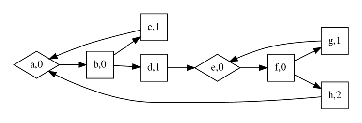
Figure 1: A reduced parity game.

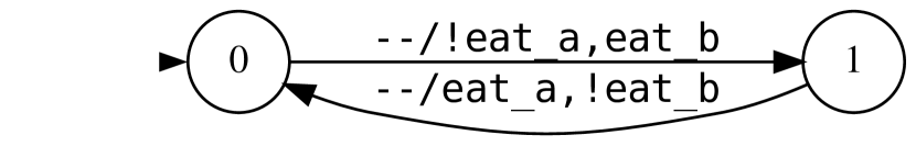
Figure 2: The resulting Mealy machine with two states, alternating $\neg eat_{A},eat_{B}$ and $eat_{A},\neg eat_{B}$ regardless of the input of $hungry_{A}$ and $hungry_{B}$.

3 Parametrized parity games

A parity game [24, 12, 31] is a two-player game of player $0$ (Even) against $1$ (Odd). We use $\alpha\in\left\{0,1\right\}$ to denote a player and ${\bar{\alpha}}$ to denote its opponent. Formally, we define a parity game as a tuple $\mathcal{PG}=(V,E,O,Pr)$ with $V$ the set of nodes, $E$ the set of possible moves represented as pairs $(v,w)$ of nodes, $O:V\to\{0,1\}$ the owner function, and $Pr$ the priority function $V\to\mathbb{N}$ mapping nodes to their priority; $(V,E)$ is also called the game graph. Each $v\in V$ has at least one possible move. We use $O_{\alpha}$ to denote nodes owned by $\alpha$.

A play (in node $v_{1}$) of the parity game is an infinite sequence of nodes $\langle v_{1},v_{2},\dots,v_{n}\dots\rangle$ where $\forall i:v_{i}\in V\land(v_{i},v_{i+1})\in E$. We use $\pi$ as a mathematical variable to denote a play. $\pi(i)$ is the $i$-th node $v_{i}$ of $\pi$. In a play $\pi$, it is the owner of the node $v_{i}$ that decides the move $(v_{i},v_{i+1})$. There exists plays in every node. We call the player $\alpha=(n\mod 2)$ the winner of priority $n$. The winner of a play is the winner of the highest priority $n$ through which the play passes infinitely often. Formally: $\mathit{Winner}(\pi)=\lim_{i\to{+\infty}}max\left\{Pr(\pi(j))\middle|j\geq i\right\}{\ \bmod\ 2}.$

The key questions for a parity game $\mathcal{PG}$ are, for each node $v$: Who is the winner? And how? As proven by [12], parity games are memoryless determined: every node has a unique winner and a corresponding memoryless winning strategy. A (memoryless) strategy for player $\alpha$ is a partial function $\sigma_{\alpha}$ from a subset of $O_{\alpha}$ to $V$. A play $\pi$ is consistent with $\sigma_{\alpha}$ if for every $v_{i}$ in $\pi$ belonging to the domain of $\sigma_{\alpha}$, $v_{i+1}$ is $\sigma_{\alpha}(v_{i})$. A strategy $\sigma_{\alpha}$ for player $\alpha$ is a winning strategy for a node $v$ if every play in $v$ consistent with this strategy is won by $\alpha$, i.e. regardless of the moves selected by ${\bar{\alpha}}$. As such, a game $\mathcal{PG}$ defines a winning function $W_{\mathcal{PG}}:V\mapsto\{0,1\}$. The set $W_{\mathcal{PG},\alpha}$ or, when $\mathcal{PG}$ is clear from the context, $W_{\alpha}$ denotes the set of nodes won by $\alpha$. Moreover, for both players $\alpha\in\{0,1\}$, there exists a memoryless winning strategy $\sigma_{\alpha}$ with domain $W_{\alpha}\cap O_{\alpha}$ that wins in all nodes won by $\alpha$. A solution of $\mathcal{PG}$ consists of a function $W^{\prime}:V\to\{0,1\}$ and two winning strategies $\sigma_{0}$ and $\sigma_{1}$, with $dom(\sigma_{\alpha})=W^{\prime}_{\alpha}\cap O_{\alpha}$, such that every play in $v\in W^{\prime}_{\alpha}$ consistent with $\sigma_{\alpha}$ is won by $\alpha$. Solutions always exist; they may differ in strategy but all have $W^{\prime}=W_{\mathcal{PG}}$, the winning function of the game. We can say that the pair $(\sigma_{0},\sigma_{1})$ proves that $W^{\prime}=W_{\mathcal{PG}}$.

In order to have a framework in which we can discuss different algorithms from the literature, we define a parametrized parity game. It consists of a parity game $\mathcal{PG}$ and a parameter function $P$, a partial function $P:V\rightharpoonup\{0,1\}$ with domain $dom(P)\subseteq V$. Elements of $dom(P)$ are called parameters, and $P$ assigns a winner to each parameter. Plays are the same as in a $\mathcal{PG}$ except that every play that reaches a parameter $v$ ends and is won by $P(v)$.

Definition 1 (Parametrized parity game)

Let $\mathcal{PG}=(V,E,O,Pr)$ be a parity game and $P:V\rightharpoonup\{0,1\}$ a partial function with domain $dom(P)\subseteq V$. Then $(\mathcal{PG},P)$ is a parametrized parity game denoted ${\mathcal{PG}_{P}}$, with parameter set $dom(P)$. If $P(v)=\alpha$, we call $\alpha$ the assigned winner of parameter $v$. The sets $P_{0}$ and $P_{1}$ denote parameter nodes with assigned winner 0 respectively 1.

A play of $(\mathcal{PG},P)$ is a sequence of nodes $\langle v_{0},v_{1},\dots\rangle$ such that for all $i$: if $v_{i}\in P_{\alpha}$ then the play halts and is won by $\alpha$, otherwise $v_{i+1}$ exists and $(v,v_{i+1})\in E$. For infinite plays, the winner is as in the original parity game $\mathcal{PG}$.

Every parity game $\mathcal{PG}$ defines a class of parametrized parity games (PPG’s), one for each partial function $P$. The original $\mathcal{PG}$ corresponds to one of these games, namely the one without parameters ($dom(P)=\emptyset$); every total function $P:V\to\{0,1\}$ defines a trivial PPG, with plays of length 0 and $P=W_{\mathcal{PG}_{P}}$.

A PPG ${\mathcal{PG}_{P}}$ can be reduced to an equivalent PG $G$: in each parameter $v\in dom(P)$ replace the outgoing edges with a self-loop and the priority of $v$ with $P(v)$. We now have a standard parity game $G$. Every infinite play $\langle v_{0},v_{1},\dots\rangle$ in ${\mathcal{PG}_{P}}$ is also an infinite play in $G$ with the same winner. Every finite play $\langle v_{0},v_{1},\dots,v_{n}\rangle$ with winner $P(v_{n})$ in ${\mathcal{PG}_{P}}$ corresponds to an infinite play $\langle v_{0},v_{1},\dots,v_{n},v_{n},\ldots\rangle$ with winner $P(v_{n})$ in $G$. Thus, the two games are equivalent. It follows that any PPG ${\mathcal{PG}_{P}}$ is a zero-sum game defining a winning function $W$ and having memory-less winning strategies $\sigma_{\alpha}$ with domain $(W_{\alpha}\setminus P_{\alpha})\cap O_{\alpha}$ (for $\alpha=0,1$).

PPG’s allow us to capture the behaviour of several state of the art algorithms as a sequence of solved PPG’s. In each step, strategies and parameters are modified and a solution for one PPG is transformed into a solution for a next PPG and this until a solution for the input PG is reached.

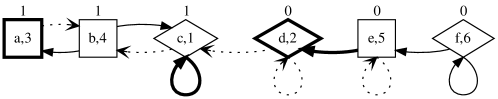
Figure 3: A parametrized parity game with nodes $a,\dots,f$, $P_{0}=\{d\}$ and $P_{1}=\{a\}$, and winning strategies for $0$ and $1$. The two parameter nodes are in bold. Square nodes are owned by Even, diamonds by Odd. The labels inside a node are the name and priority; the label on top of a node is the winner. A bold edge belongs to a winning strategy (of the owner of its start node). A slim edge is one starting in a node that is lost by its owner. All remaining edges are dotted.

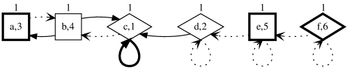
Figure 4: A parametrized parity game and strategy, after withdrawing $d$ from the parameter list.

Example 1

Figure 3 shows a parametrized parity game and its winning strategies. The parameter nodes $a$ and $d$ are won by the assigned winners, respectively 1 and 0. Player 1 owns node $c$ and wins its priority. Hence, by playing from $c$ to $c$, 1 wins in this node. Node $b$ is owned by 0 but has only moves to nodes won by 1, hence it is also won by 1. Player 0 wins node $e$ by playing to node $d$; 1 plays in node $f$ but playing to $f$ results in an infinite path won by 0, while playing to node $e$ runs into a path won by 0, so $f$ is won by 0.

Based on this PPG, we can construct a solved PPG where node $d$ is removed from the parameters. The strategy is adjusted accordingly: Odd wins in $d$ by playing to $c$ . However, changing the winner of $d$ breaks the strategies and winners of the nodes $e$ and $f$. Figure 4 shows one way to obtain a solved PPG with further adjustments: nodes $e$ and $f$ are turned into parameters won by $1$. Many other solutions exist, e.g., by turning $e$ into a parameter won by $0$.

4 Justifications

In Figure 3 and Figure 4, the solid edges form the subgraph of the game graph that was analysed to confirm the winners of all nodes. We formalize this subgraph as a justification, a concept introduced in [15] and described below. In the rest of the paper, we assume the existence of a parity game $\mathcal{PG}=(V,E,O,Pr)$ and a parametrized parity game $\mathcal{PG}_{P}=(\mathcal{PG},P)$ with $P$ a parameter function with set of parameters $dom(P)$. Also, we use $H:V\to\{0,1\}$ as a function describing a “hypothesis” of who is winning in the nodes.

Definition 2 (Direct justification)

A direct justification $dj$ for player $\alpha$ to win node $v$ is a set containing one outgoing edge of $v$ if $O(v)=\alpha$ and all outgoing edges of $v$ if $O(v)={\bar{\alpha}}$.

A direct justification $dj$ wins $v$ for $\alpha$ under hypothesis $H$ if for all $(v,w)\in dj$, $H(w)=\alpha$. We also say: $\alpha$ wins $v$ by $dj$ under $H$.

Definition 3 (Justification)

A justification $J$ for $\mathcal{PG}$ is a tuple $(V,D,H)$ such that $(V,D)$ is a subgraph of $(V,E)$. If a node has outgoing edges in $D$, it is justified in $J$, otherwise it is unjustified.

Definition 4 (Weakly winning)

A justification $(V,D,H)$ is weakly winning if for all justified nodes $v\in V$ the set of outgoing edges $Out_{v}$ is a direct justification that wins $v$ for $H(v)$ under $H$.

We observe that any justification $J=(V,D,H)$ determines a PPG $\mathcal{PG}_{P_{J}}$ where the parameter function $P_{J}$ is the restriction of $H$ to unjustified nodes.

If $J$ is weakly winning, the set of edges $\{(v,w)\in D\mid O(v)=H(v)=\alpha\}$ is a partial function on $O_{\alpha}$, i.e., a strategy for $\alpha$. We denote it as $\sigma_{J,\alpha}$.

Proposition 1

Assume a weakly winning justification $J=(V,D,H)$. Then, (i) For every path $\pi$ in $D$, all nodes $v$ on $\pi$ have the same hypothetical winner $H(v)$. (ii) All finite paths $\pi$ starting in node $v$ in $D$ are won in $\mathcal{PG}_{P_{J}}$ by $H(v)$. (iii) Every path in $D$ with nodes hypothetically won by $\alpha$ is consistent with $\sigma_{J,\alpha}$. (iv) Every play starting in $v$ of $\mathcal{PG}_{P_{J}}$ consistent with $\sigma_{J,H(v)}$ is a path in $D$.

Proof

(i) Since any edge $(v,w)\in D$ belongs to a direct justification that wins $v$ for $H(v)$, it holds that $H(v)=H(w)$. It follows that every path $\pi$ in $D$ consists of nodes with the same hypothetical winner. (ii) If path $\pi$ in $v$ is finite and ends in parameter $w$, then $H(v)=H(w)$. The winner of $\pi$ in $\mathcal{PG}_{P_{J}}$ is $P_{J}(w)$ which is equal to $H(v)$ as $H$ expands $P_{J}$. (iii) Every path in $D$ with hypothetical winner $\alpha$, follows $\sigma_{J,\alpha}$ when it is in a node $v$ with owner $\alpha$. (iv) Let $H(v)=\alpha$ and $\pi$ be a play in $v$ of ${\mathcal{PG}_{P}}$ consistent with $\sigma_{J,\alpha}$. We can inductively construct a path from $v=v_{1}$ in $D$. It follows from (i) that the $n$’th node $v_{n}$ has $H(v_{n})=H(v_{1})=\alpha$. For each non-parameter node $v_{n}$, if $O(v_{n})=\alpha$, then $v_{i+1}=\sigma_{J,\alpha}(v_{i})$ which is in $D$. If $O(v_{n})={\bar{\alpha}}$ then $D$ contains all outgoing edges from $v_{n}$ including the one to $v_{n+1}$. ∎

Definition 5 (Winning)

A justification $J=(V,D,H)$ is winning if (i) $J$ is weakly winning and (ii) all infinite paths $\langle v_{1},v_{2},\dots\rangle$ in $D$ are plays of $\mathcal{PG}$ won by $H(v_{1})$.

Observe that, if $J$ is winning and $H(v)=\alpha$, all plays in $\mathcal{PG}_{P_{J}}$ starting in $v$ and consistent with $\sigma_{(V,D,H),\alpha}$ are paths in $(V,D)$ won by $\alpha$. Hence:

Theorem 4.1

If $J=(V,D,H)$ is a winning justification for $\mathcal{PG}_{P_{J}}$ then $H$ is $W_{\mathcal{PG}_{P_{J}}}$, the winning function of $\mathcal{PG}_{P_{J}}$, with corresponding winning strategies $\sigma_{J,0}$ and $\sigma_{J,1}$.

The central invariant of the algorithm presented below is that its data structure $J=(V,D,H)$ is a winning justification. Thus, in every stage, $H$ is the winning function of $\mathcal{PG}_{P_{J}}$ and the graph $(V,D)$ comprises winning strategies $\sigma_{J,\alpha}$ for both players. In a sense, $(V,D)$ provides a proof that $H$ is $W_{\mathcal{PG}_{P_{J}}}$.

4.1 Operations on weakly winning justifications

We introduce an operation that modifies a justification $J=(V,D,H)$ and hence also the underlying game $\mathcal{PG}_{P_{J}}$. Let $v$ be a node in $V$, $\alpha$ a player and $dj$ either the empty set or a direct justification. We define $J[v:dj,\alpha]$ as the justification $J^{\prime}=(V,D^{\prime},H^{\prime})$ where $D^{\prime}$ is obtained from $D$ by replacing the outgoing edges of $v$ by the edges in $dj$, and $H^{\prime}$ is the function obtained from $H$ by setting $H^{\prime}(v):=\alpha$. Modifications for a set of nodes are independent of application order. E.g., $J[v:\emptyset,H^{\prime}(v)\mid v\in S]$ removes all out-going edges of $v$ and sets $H^{\prime}(v)$ for all $v\in S$. Multiple operations, like $J[v:dj,\alpha][v^{\prime}:dj^{\prime},\alpha^{\prime}]$, are applied left to right. Some useful instances, with their properties, are below.

In the proposition, a cycle in $J$ is a finite sequence of nodes following edges in $J$ that ends in its starting node.

Proposition 2

For a weakly winning justification $J$ and a node $v$ with direct justification $dj$ the following holds:

(i) If $H(v)={\bar{\alpha}}$, $v$ has no incoming edges and $dj$ wins $v$ for $\alpha$ under $H$, then $J[v:dj,\alpha]$ is weakly winning and there are no cycles in $J^{\prime}$ with edges of $dj$.

(ii) Let $S$ be a set of nodes closed under incoming edges (if $v\in S$ and $(w,v)\in D$, then $w\in S$), let $H_{f}$ be an arbitrary function mapping nodes of $S$ to players. It holds that $J[v:\emptyset,H_{f}(v)\mid v\in S]$ is weakly winning. There are no cycles in $J^{\prime}$ with edges of $dj$.

(iii) If $H(v)=\alpha$ and $dj$ wins $v$ for $\alpha$ under $H$, then $J[v:dj,\alpha]$ is weakly winning. There are no new cycles when $(v,v)\not\in dj$ and no $w\in range(dj)$ can reach $v$ in $J$. Otherwise new cycles pass through $v$ and have at least one edge in $dj$.

Proof

We exploit the fact that $J$ and $J^{\prime}$ are very similar.

(i) The direct justification $dj$ cannot have an edge ending in $v$ since $H(v)\neq H(w)$ for $(v,w)\in dj$ and no $w\in dj$ can reach $v$ in $J$ since $v$ has no incoming edges, hence $J^{\prime}$ has no cycles through $dj$. As $J$ is weakly winning and $H$ is updated only in $v$, the direct justification of a justified node $w\neq v$ in $J$ is still winning in $J^{\prime}$. Since also $dj$ wins $v$ for $\alpha$, $J^{\prime}$ is weakly winning.

(ii) Setting $H(v)$ arbitrary cannot endanger the weak support of $J^{\prime}$ as $v$ has no direct justification and no incoming edges in $J^{\prime}$. Hence $J^{\prime}$ is weakly winning. Also, removing direct justifications cannot introduce new cycles.

(iii) Let $H(v)=\alpha$ and $dj$ wins $v$ for $\alpha$ under $H$. Let $J^{\prime}=J[v:dj,\alpha]$. We have $H^{\prime}=H$ so the direct justifications of all nodes $w\neq v$ in $J^{\prime}$ win $w$ for $H^{\prime}(w)$. Since $dj$ wins $v$ for $H^{\prime}(v)$, $J^{\prime}$ is weakly winning. Also, new cycles if any, pass through $dj$ and $v$.

4.2 Constructing winning justifications

The eventual goal of a justification is to create a winning justification without unjustified nodes. Such a justification contains a solution for the parity game without parameters. To reach this goal we start with an empty winning justification and iteratively assign a direct justification to one of the nodes.

However, haphazardly (re)assigning direct justifications will violate the intended winning justification invariant. Three problems appear: First, changing the hypothesis of a node may violate weakly winning for incoming edges. The easiest fix is to remove the direct justification of nodes with edges to this node. Yet removing direct justifications decreases the justification progress. Thus a second problem is ensuring progress and termination despite these removals. Third, newly created cycles must be winning for the hypothesis. To solve these problems, we introduce safe justifications; we start with some auxiliary concepts.

Let $J$ be a justification. The set of nodes reaching $v$ in J, including $v$, is closed under incoming edges and is denoted with $J{\downarrow_{v}}$. The set of nodes reachable from $v$ in $J$, including $v$, is denoted with $J{\uparrow_{v}}$. We define $\mathit{Par}_{J}(v)$ as the parameters reachable from the node $v$, formally $\mathit{Par}_{J}(v)=J{\uparrow_{v}}\cap dom(P)$. The justification level $jl_{J}(v)$ of a node $v$ is the lowest priority of all its parameters and $+\infty$ if $v$ has none. The justification level $jl_{J}(dj)$ of a direct justification $dj=\{(v,w_{1}),\ldots,(v,w_{n})\}$ is $min\{jl_{J}(w_{1}),\ldots,jl_{J}(w_{n})\}$, the minimum of the justification levels of the $w_{i}$. We drop the subscript $J$ when it is clear from the context and write $\mathit{Par}(v)$, $jl(v)$ and $jl(dj)$ for the above concepts. The default winner of a node $v$ is the winner of its priority, i.e., $Pr(v){\ \bmod\ 2}$; the default hypothesis $H_{d}$ assigns default winners to all nodes, i.e., $H_{d}(v)=Pr(v){\ \bmod\ 2}$.

Definition 6 (Safe justification)

A justification is safe iff (i) it is a winning justification, (ii) all unjustified nodes $v$ have $H(v)={H_{d}}(v)$, that is, the winners of the current parameters of the PPG are their default winners, and (iii) $\forall v\in V:jl(v)\geq Pr(v)$, i.e., the justification level of a node is at least its priority.

Fixing the invariants is easier for safe justifications. Indeed, for nodes $w$ on a path to a parameter $v$, $Pr(v)\geq jl(w)\geq Pr(w)$, so when $v$ is given a direct justification to $w$ then $Pr(v)$ is the highest priority in the created cycle and $H(v)$ correctly denotes its winner. Furthermore, the empty safe justification $(V,\emptyset,{H_{d}})$ will serve as initialisation of the solving process.

4.3 The operation Justify

To progress towards a solution, we introduce a single operation, namely ${{\bf Justify}}$. Given appropriate inputs, it can assign a direct justification to an unjustified node or replace the direct justification of a justified node. Furthermore, if needed, it manipulates the justification in order to restore its safety.

Definition 7 (Justify)

The operation ${{\bf Justify}}(J,v,dj)$ is executable if

• Precondition 1: $J=(V,D,H)$ is a safe justification, $v$ is a node in $V$, there exists a player $\alpha$ who wins $v$ by $dj$ under $H$.

• Precondition 2: if $v$ is unjustified in $J$ then $jl(dj)\geq jl(v)$ else $jl(dj)>jl(v)$.
  

Let ${{\bf Justify}}(J,v,dj)$ be executable. If $H(v)=\alpha$ then ${{\bf Justify}}(J,v,dj){}=J[v:dj,H(v)]$, i.e., $dj$ becomes the direct justification of $v$.

If $H(v)={\bar{\alpha}}$, then ${{\bf Justify}}(J,v,dj){}={J[w:\emptyset,{H_{d}}(w)\mid w\in J{\downarrow_{v}}][v:dj,\alpha]}$, i.e., $\alpha$ wins $v$ by $dj$, while all other nodes $w$ that can reach $v$ become unjustified, and their hypothetical winner $H(w)$ is reset to their default winner.

If ${{\bf Justify}}(J,v,dj)$ is executable, we say that $v$ is justifiable with $dj$ or justifiable for short; when performing the operation, we justify $v$.

Observe, when Justify modifies the hypothetical winner $H(v)$, then, to preserve weak winning, edges $(w,v)$ need to be removed, which is achieved by removing the direct justification of $w$. Moreover, to preserve (iii) of safety, this process must be iterated until fixpoint and to preserve (ii) of safety, the hypothetical winner $H(w)$ of $w$ needs to be reset to its default winner. This produces a situation satisfying all invariants. Furthermore, when Justify is applied on a justified $v$, it preserves $H(v)$ but it replaces $v$’s direct justification by one with a strictly higher justification level. As the proof below shows, this ensures that no new cycles are created through $v$ so we can guarantee that all remaining cycles still have the correct winner. So, cycles can only be created by justifying an unjustified node.

Lemma 1

An executable operation ${{\bf Justify}}(J,v,dj)$ returns a safe justification.

Proof

Assume ${{\bf Justify}}(J,v,dj)$ is executable, $J^{\prime}={{\bf Justify}}(J,v,dj)$ and let $\alpha$ be the player that wins $v$ by $dj$. First, we prove that $J^{\prime}$ is also a winning justification, i.e., that $J^{\prime}$ is weakly winning and that the winner of every infinite path in $J^{\prime}$ is the hypothetical winner $H(w)$ of the nodes $w$ on the path.

The operations applied to obtain $J^{\prime}$ are the ones that have been analysed in Proposition 2 and for which it was proven that they preserve weakly winning. Note that, in case $H(v)={\bar{\alpha}}$, the intermediate justification $J[v:\emptyset,{H_{d}}(v)\mid v\in J{\downarrow_{v}}]$ removes all incoming edges of $v$. Hence, $J^{\prime}$ is weakly winning and all nodes $v,w$ connected in $J$ have $H^{\prime}(v)=H^{\prime}(w)$ (*). If no edge in $dj$ belongs to a cycle, then every infinite path $\langle v_{1},v_{2},\dots\rangle$ in $J^{\prime}$ has an infinite tail in $J$ starting in $w\neq v$ which is, since $J$ is winning, won by $H(w)$. By (*), this path is won by $H(v_{1})=H(w)$ and $J^{\prime}$ is winning.

If $J^{\prime}$ has cycles through edges in $dj$, then, by (i) of Proposition 2, $H(v)$ must be $\alpha$ and we are in case (iii) of Proposition 2. We analyse the nodes $n$ on such a cycle. By safety of $J$, $Pr(n)\leq jl_{J}(n)$; as $n$ reaches $v$ in $J$, $jl_{J}(n)\leq jl_{J}(v)$. If $v$ is unjustified in $J$ then $jl_{J}(v)=Pr(v)\geq Pr(n)$, hence $Pr(v)$ is the highest priority on the cycle and $H(v)$ wins the cycle. If $v$ is justified in $J$ and $(v,w)\in dj$ is on the new cycle, then $jl_{J}(w)\geq jl_{J}(dj)>jl_{J}(v)$ (Precondition 2 of Justify). But $w$ reaches $v$ so $jl_{J}(w)\leq jl_{J}(v)$ , which is a contradiction.

Next, we prove that J’ is a safe justification (Definition 6). (i) We just proved that $J^{\prime}$ is a winning justification. (ii) For all unjustified nodes $v$ of $J^{\prime}$, it holds that $H(v)={H_{d}}(v)$, its default winner. Indeed, $J$ has this property and whenever the direct justification of a node $w$ is removed, $H^{\prime}(w)$ is set to ${H_{d}}(w)$.

(iii) We need to prove that for all nodes $w$, it holds that $jl_{J^{\prime}}(w)\geq Pr(w)$. We distinguish between the two cases of ${{\bf Justify}}(J,v,dj)$.

(a) Assume $H(v)=\alpha=H^{\prime}(v)$ and $J^{\prime}=J[v:dj,H(v)]$ and let $w$ be an arbitrary node of $V$. If $w$ cannot reach $v$ in $J^{\prime}$, the parameters that $w$ reaches in $J$ and $J^{\prime}$ are the same and it follows that $jl_{J^{\prime}}(w)=jl_{J}(w)\geq Pr(w)$. So, (iii) holds for $w$. Otherwise, if $w$ reaches $v$ in $J^{\prime}$, then $w$ reaches $v$ in $J$ and any parameter $x$ that $w$ reaches in $J^{\prime}$ is a parameter that $w$ reaches in $J$ or one that an element of $dj$ reaches in $J$. It follows that $jl_{J^{\prime}}(w)$ is at least the minimum of $jl_{J}(w)$ and $jl_{J}(dj)$. As $w$ reaches $v$ in $J$, $jl_{J}(w)\leq jl_{J}(v)$. Also, by Precondition 2 of Justify, $jl_{J}(v)\leq jl_{J}(dj)$. It follows that $jl_{J^{\prime}}(w)\geq jl_{J}(w)\geq Pr(w)$. Thus, (iii) holds for $w$.

(b) Assume $H^{\prime}(v)\neq H(v)={\bar{\alpha}}$ and $J^{\prime}=J[w:\emptyset,{H_{d}}(w)\mid w\in J{\downarrow_{v}}][v:dj,\alpha]$ then for nodes $w$ that cannot reach $v$ in $J$, $\mathit{Par}_{J^{\prime}}(w)=\mathit{Par}_{J}(w)$ hence $jl_{J^{\prime}}(w)=jl_{J}(w)\geq Pr(w)$ and (iii) holds for $w$. All nodes $w\neq v$ that can reach $v$ in $J$ are reset, hence $jl_{J^{\prime}}(w)=Pr(w)$ and (iii) holds. As for $v$, by construction $jl_{J^{\prime}}(v)=jl_{J}(dj)\geq jl_{J}(v)$; also $jl_{J}(v)\geq Pr(v)$ hence (iii) also holds. ∎

Lemma 2

Let $J$ be a safe justification for a parametrized parity game. Unless $J$ defines the parametrized parity game $PG_{\emptyset}=\mathcal{PG}$, there exists a node $v$ justifiable with a direct justification $dj$, i.e., such that ${{\bf Justify}}(J,v,dj)$ is executable.

Proof

If $J$ defines the parametrized parity game $PG_{\emptyset}$ then all nodes are justified and $J$ is a solution for the original $\mathcal{PG}$. Otherwise let $p$ be the minimal priority of all unjustified nodes, and $v$ an arbitrary unjustified node of priority $p$ and let its owner be $\alpha$. Then either $v$ has an outgoing edge $(v,w)$ to a node $w$ with $H(w)=\alpha$, thus a winning direct justification for $\alpha$, or all outgoing edges are to nodes $w$ for which $H(w)={\bar{\alpha}}$, thus $v$ has a winning direct justification for ${\bar{\alpha}}$. In both cases, this direct justification $dj$ has a justification level larger or equal to $p$ since no parameter with a smaller priority exist, so ${{\bf Justify}}(J,v,dj)$ is executable. ∎

To show progress and termination, we need an order over justifications.

Definition 8 (Justification size and order over justifications)

Let $1,\ldots,n$ be the range of the priority function of a parity game $PG$ ( ${+\infty}>n$) and $J$ a winning justification for a parametrized parity game extending $PG$. The size of $J$, $s(J)$ is the tuple $(s_{{+\infty}}(J),s_{n}(J),\ldots s_{1}(J))$ where for $i\in\{1,\dots,n,+\infty\}$, $s_{i}(J)$ is the number of justified nodes with justification level $i$.

The order over justifications is the lexicographic order over their size: with $i$ the highest index such that $s_{i}(J)\neq s_{i}(J^{\prime})$, we have $J>_{s}J^{\prime}$ iff $s_{i}(J)>s_{i}(J^{\prime})$.

The order over justifications is a total order which is bounded as $\Sigma_{i}s_{i}(J)\leq|V|$.

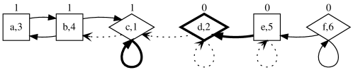
Figure 5: Above, in solid line the edges of the justification graph of the winning but unsafe justification of Figure 3 and below the result of justifying node $a$, a non-winning justification.

Example 2

Let us revisit Example 1. The winning justification $J$ of Figure 3 is shown at the top of Figure 5. For the justified nodes of $J$, we have $jl(b)=3$, $jl(c)=+\infty$, $jl(e)=2$ and $jl(f)=2$. The justification is not safe as, e.g., $jl(b)=3<Pr(b)=4$. Both unjustified nodes $a$ and $d$ have a winning direct justification, the direct justification $\{(a,b)\}$ wins $a$ for player 1 and the direct justification $\{(d,c)\}$ wins $d$ for 1. The figure at the bottom shows the justification resulting from inserting the direct justification winning $a$. There is now an infinite path $\langle a,b,a,b,\ldots\rangle$ won by Even but with nodes with hypothetical winner Odd. The justification ${{\bf Justify}}(J,a,\left\{(a,b)\right\})$ is not winning. This shows that condition (iii) of safety of $J$ is a necessary precondition for maintaining the desired invariants.

Lemma 3

Let $J$ be a safe justification with size $s_{J}$, $v$ a node justifiable with $dj$ and $J^{\prime}={{\bf Justify}}(J,v,dj){}$ a justification with size $s_{J^{\prime}}$. Then $s_{J^{\prime}}>s_{J}$.

Proof

In case $v$ is unjustified in $J$ and is assigned a $dj$ that wins $v$ for $H(v)$, $v$ is not counted for the size of $J$ but is counted for the size of $J^{\prime}$. Moreover, other nodes keep their justification level (if they cannot reach $v$ in $J$) or may increase their justification level (if they can reach $v$ in $J$). In any case, $s_{J^{\prime}}>s_{J}$.

In case $v$ is justified in $J$ and is assigned a $dj$ that wins $v$ for $H(v)$, then $jl_{J}(dj)>jl_{J}(v)$, so $jl_{J}^{\prime}(v)>jl_{J}(v)$. Other nodes keep their justification level or, if they reach $v$, may increase their justification level. Again, $s_{J^{\prime}}>s_{J}$.

Finally, the case where $dj$ wins $v$ for the opponent of $H(v)$. Nodes can be reset; these nodes $w$ have $jl_{J}(w)\leq Pr(v)$. As a node cannot have a winning direct justification for both players, $v$ is unjustified in $J$. Hence, by precondition (2) of Justify, $jl_{J}(dj)\geq Pr(v)$. In fact, it holds that $jl_{J}(dj)>Pr(v)$. Indeed, if some $w\in dj$ would have a path to a parameter of $v$’s priority, that path would be won by ${H_{d}}(v)=H(v)$ while $H(w)$ is its opponent. Thus, the highest index $i$ where $s_{i}$ changes is $jl_{J}(dj)$, and $s_{i}$ increases. Hence, $s_{J^{\prime}}>s_{J}$. ∎

Theorem 4.2

Any iteration of Justify steps from a safe justification, in particular from $(V,\emptyset,{H_{d}})$, with ${H_{d}}$ the default hypothesis, eventually solves $\mathcal{PG}$.

Proof

By induction: Let $\mathcal{PG}=(V,E,O,Pr)$ be a parity game. Clearly, the empty justification $J^{0}=(V,\emptyset,{H_{d}})$ is a safe justification. This is the base case.

Induction step: Let $J^{i}$ be the safe justification after $i$ successful Justify steps and assume that $J^{i}=(V,D^{i},H^{i})$ contains an unjustified node. By Lemma 2, there exists a pair $v$ and $dj$ such that $v$ is justifiable with $dj$. For any pair $v$ and $dj$ such that ${{\bf Justify}}(J^{i},v,dj)$ is executable, let $J^{i+1}={{\bf Justify}}(J^{i},v,dj)$. By Lemma 1, $J^{i+1}$ is a safe justification. By Lemma 3, there is a strict increase in size, i.e., $s(J^{i+1})>s(J^{i})$.

Since the number of different sizes is bounded, this eventually produces a safe $J^{k}=(V,D^{k},H^{k})$ without unjustified nodes. The parametrized parity game $\mathcal{PG}_{P_{J^{k}}}$ determined by $J^{k}$ is $\mathcal{PG}$. Hence, $H^{k}$ is the winning function of $\mathcal{PG}$, and $J^{k}$ comprises winning strategies for both players. ∎

Theorem 4.2 gives a basic algorithm to solve parity games. The algorithm has three features: it is (1) simple, (2) nondeterministic, and (3) in successive steps it may arbitrarily switch between different priority levels. Hence, by imposing different strategies, different instantiations of the algorithm are obtained.

Existing algorithms differ in the order in which they (implicitly) justify nodes. In the next section we simulate such algorithms by different strategies for selecting nodes to be justified. Another difference between algorithms is in computing the set $R$ of nodes that is reset when $dj$ wins $v$ for the opponent of $H(v)$. Some algorithms reset more nodes; the largest reset set for which the proofs in this paper remain valid is $\{w\in V\mid jl(w)<jl(dj)\}$. To the best of our knowledge, the only algorithms that reset as few nodes as ${{\bf Justify}}(J,v,dj)$ are the ones we presented in [21]. As the experiments presented there show, the work saved across iterations by using justifications results in better performance.

5 A reformulation of three existing algorithms

In this section, by ordering justification steps, we obtain basic versions of different algorithms known from the literature. In our versions, we represent the parity game $G$ as $(V,E,O,Pr)$ and the justification J as $(V,D,H)$. All algorithms start with the safe empty justification $(V,\emptyset,{H_{d}})$. The recursive algorithms operate on a subgame $SG$ determined by a set of nodes $V_{SG}$. This subgame determines the selection of ${{\bf Justify}}(J,v,dj)$ steps that are performed on $G$. For convenience of presentation, $G$ is considered as a global constant.

5.0.1 Nested fixpoint iteration [7, 11, 21]

is one of the earliest algorithms able to solve parity games. In Algorithm 1, we show a basic form that makes use of our ${{\bf Justify}}(J,v,dj)$ action. It starts from the initial justification $(V,\emptyset,H_{d})$. Iteratively, it determines the lowest priority $p$ over all unjustified nodes, it selects a node $v$ of this priority and justifies it. Recall from the proof of Lemma 2, that all unjustified nodes of this priority are justifiable. Eventually, all nodes are justified and a solution is obtained. For more background on nested fixpoint algorithms and the effect of justifications on the performance, we refer to our work in [21].

A feature of nested fixpoint iteration is that it solves a parity game bottom up. It may take many iterations before it uncovers that the current hypothesis of some high priority unjustified node $v$ is, in fact, wrong and so that playing to $v$ is a bad strategy for $\alpha$. The next algorithms are top down, they start out from nodes with the highest priority.

1 Fn ${{\bf Fixpoint}}(G)$:

2      $J\textnormal{{$\leftarrow$}}(V,\emptyset,{H_{d}})$ the initial safe justification

3      while $J$ has unjustified nodes do

4           $p\textnormal{{$\leftarrow$}}min\left\{Pr(v)\ \middle|\ v\text{ is unjustified}\right\}$

5           $v\textnormal{{$\leftarrow$}}$ an unjustified node with $Pr(v)=p$

6           ${dj}\textnormal{{$\leftarrow$}}$ a winning direct justification for $v$ under $H$

7           $J\textnormal{{$\leftarrow$}}{{\bf Justify}}(J,v,{dj})$

8          

9     return $J$

Algorithm 1 A fixpoint algorithm for justifying nodes

input : A parity game $G$

1 $J\textnormal{{$\leftarrow$}}{{\bf Zielonka}}((V,\emptyset,{H_{d}}),V)$

2 Fn ${{\bf Zielonka}}(J,V_{SG})$:

3      $p\textnormal{{$\leftarrow$}}max\left\{Pr(v)\ \middle|\ v\in V_{SG}\right\}$

4      $\alpha\textnormal{{$\leftarrow$}}p{\ \bmod\ 2}$

5      while $true$ do

6           while $\exists v\in V_{SG},dj:v$ is unjustified, $v$ is justifiable with ${dj}$ for $\alpha$ with $jl({dj})\geq p$  do

7                $J\textnormal{{$\leftarrow$}}{{\bf Justify}}(J,v,{dj})$

8               

9          $V_{SSG}\textnormal{{$\leftarrow$}}\{v\in V_{SG}|Pr(v)<p,$

10                        $v$ is unjustified}

11           if $V_{SSG}=\emptyset$ then return $J$;

12           $J\textnormal{{$\leftarrow$}}{{\bf Zielonka}}(J,V_{SSG})$

13           while $\exists v\in V_{SG},dj:v$ is unjustified, $v$ is justifiable with ${dj}$ for ${\bar{\alpha}}$ with $jl({dj})\geq p+1$  do

14                $J\textnormal{{$\leftarrow$}}{{\bf Justify}}(J,v,{dj})$

15               

Algorithm 2 A Justify variant of Zielonka’s algorithm.

5.0.2 Zielonka’s algorithm [32],

one of the oldest algorithms, is recursive and starts with a greedy computation of a set of nodes, called attracted nodes, in which the winner $\alpha$ of the top priority $p$ has a strategy to force playing to nodes of top priority $p$. In our reconstruction, Algorithm 2, attracting nodes is simulated at Line 2 by repeatedly justifying nodes $v$ with a direct justification that wins $v$ for $\alpha$ and has a justification level $\geq p$. Observe that the while test ensures that the preconditions of ${{\bf Justify}}(J,v,dj)$ on the justification level of $v$ are satisfied. Also, every node can be justified at most once.

The procedure is called with a set $V_{SG}$ of nodes of maximal level $p$ that cannot be attracted by levels $>p$. It follows that the subgraph determined by $V_{SG}$ contains for each of its nodes an outgoing edge (otherwise the opponent of the owner of the node would have attracted the node at a level $>p$) , hence this subgraph determines a parity game. The main loop invariants are that (1) the justification $J$ is safe; (2) the justification level of all justified nodes is $\geq p$ and (3) ${\bar{\alpha}}$ has no direct justifications of justification level $>p$ to win an unjustified node in $V_{SG}$. The initial justification is safe and it remains so as every ${{\bf Justify}}$ call satisfies the preconditions.

After the attraction loop at Line 2, no more unjustified nodes of $V_{SG}$ can be attracted to level $p$ for player $\alpha$. Then, the set of $V_{SSG}$ of unjustified nodes of priority $<p$ is determined. If this set is empty, then by Lemma 2 all unjustified nodes of priority $p$ are justifiable with a direct justification $dj$ with $jl(dj)\geq p$, hence they would be attracted to some level $\geq p$ which is impossible. Thus, there are no unjustified nodes of priority $p$. In this case, the returned justification $J$ justifies all elements of $V_{SG}$. Else, $V_{SSG}$ is passed in a recursive call to justify all its nodes. Upon return, if ${\bar{\alpha}}$ was winning some nodes in $V_{SSG}$, their justification level will be $\geq p+1$. Now it is possible that some unjustified nodes of priority $p$ can be won by ${\bar{\alpha}}$ and this may be the start of a cascade of resets and attractions for ${\bar{\alpha}}$. The purpose of Line 2 is to attract nodes of $V_{SG}$ for ${\bar{\alpha}}$. Note that ${{\bf Justify}}(J,v,dj)$ resets all nodes that depend on nodes that switch to ${\bar{\alpha}}$. When the justification returned by the recursive call shows that $\alpha$ wins all nodes of $V_{SSG}$, the yet unjustified nodes of $V_{SG}$ are of priority $p$, are justifiable by Lemma 2 and can be won only by $\alpha$. So, at the next iteration, the call to $Attr_{\alpha}$ will justify all of them for $\alpha$ and $V_{SSG}$ will be empty. Eventually the initial call of Line 2 finishes with a safe justification in which all nodes are justified thus solving the game $G$.

Whereas fixpoint iteration first justifies low priority nodes resulting in low justification levels, Zielonka’s algorithm first justifies nodes attracted to the highest priority. Compared to fixpoint iteration, this results in large improvements in justification size which might explain its better performance. However, Zielonka’s algorithm still disregards certain opportunities for increasing justification size as it proceeds by priority level, only returning to level $p$ when all sub-problems at level $<p$ are completely solved. Indeed, some nodes computed at a low level $i<\!\!<p$ may have a very high justification level, even $+\infty$ and might be useful to revise false hypotheses at high levels, saving much work, but this is not exploited. The next algorithm, priority promotion, overcomes this limitation.

5.0.3 Priority promotion [3, 2, 4]

follows the strategy of Zielonka’s algorithm except that, when it detects that all nodes for priority $p$ are justified, it does not make a recursive call but returns the set of nodes attracted to priority $p$ nodes as a set $R_{p}$ to a previous level $q$. There $R_{p}$ is added to the attraction set at level $q$ and the attraction process is restarted. In the terminology of [3], the set $R_{p}$ is a closed $p$-region that is promoted to level $q$. A closed $p$-region of $V_{SG}$, with maximal priority $p$, is a subset $R_{p}\subseteq V_{SG}$ that includes all nodes of $V_{SG}$ with priority $p$ and for which $\alpha=p{\ \bmod\ 2}$ has a strategy winning all infinite plays in $R_{p}$ and for which ${\bar{\alpha}}$ cannot escape from $R_{p}$ unless to nodes of higher $q$-regions won by $\alpha$. We call the latter nodes the escape nodes from $R_{p}$ denote the set of them as $Escape(R_{p})$. The level to which $R_{p}$ is promoted is the lowest $q$-region that contains an escape node from $R_{p}$. It is easy to show that $q$ is a lower bound of the justification level of $R_{p}$. In absence of escape nodes, $R_{p}$ is promoted to $+\infty$.

input : A parity game $G$

1 $J\textnormal{{$\leftarrow$}}(V,\emptyset,{H_{d}})$

2 while $\exists v\in V_{G}:v$ is unjustified do

3      $R_{+\infty}\textnormal{{$\leftarrow$}}\left\{v\ \middle|\ jl(v)=+\infty\right\}$

4      $V_{SG}\textnormal{{$\leftarrow$}}V\setminus R_{+\infty}$

5      $(J,\_,\_)\textnormal{{$\leftarrow$}}{{\bf Promote}}(V_{SG},J)$

6      while $\exists v\in V_{SG},dj:v$ is justifiable with ${dj}$ and $jl({dj})=+\infty$ do

7           $J\textnormal{{$\leftarrow$}}{{\bf Justify}}(J,v,{dj})$

8          

Algorithm 3 A variant of priority promotion using Justify.

1 Fn ${{\bf Promote}}(V_{SG},J)$:

2      $p\textnormal{{$\leftarrow$}}max\left\{Pr(v)\ \middle|\ v\in V_{SG}\right\}$

3      $\alpha\textnormal{{$\leftarrow$}}p{\ \bmod\ 2}$

4      while $true$ do

5           while $\exists v\in V_{SG},dj:v$ is unjustified or $jl(v)<p$, $v$ is justifiable with ${dj}$ for $\alpha$ with $jl({dj})\geq p$  do

6                $J\textnormal{{$\leftarrow$}}{{\bf Justify}}(J,v,{dj})$

7          $R_{p}\textnormal{{$\leftarrow$}}\left\{v\in V_{SG}\ \middle|\ jl(v)\geq p\right\}$

8           if ${{\bf Closed}}(R_{p},V_{SG})$ then

9                $l\textnormal{{$\leftarrow$}}min\{q|R_{q}$ contains an escape node of $R_{p}\}$

10                return $(J,R_{p},l)$

11          $V_{SSG}\textnormal{{$\leftarrow$}}V_{SG}\setminus R_{p}$

12           $(J,R_{p^{\prime}},l)\textnormal{{$\leftarrow$}}{{\bf Promote}}(V_{SSG},J)$

13           if $l>p$ then

14               return $(J,R_{p^{\prime}},l)$

15          

Our variant of priority promotion (PPJ) is in Algorithm 3. Whereas Zielonka returned a complete solution $J$ on $V_{SG}$, Promote returns only a partial $J$ on $V_{SG}$; some nodes of $V_{SG}$ may have an unfinished justification ($jl(v)<+\infty$). To deal with this, Promote is iterated in a while loop that continues as long as there are unjustified nodes. Upon return of Promote, all nodes attracted to the returned $+\infty$-region are justified. In the next iteration, all nodes with justification level $+\infty$ are removed from the game, permanently. Note that when promoting to some $q$-region, justified nodes of justification level $<q$ can remain. A substantial gain can be obtained compared to the original priority promotion algorithm which does not maintain justifications and loses all work stored in $J$.

By invariant, the function Promote is called with a set of nodes $V_{SG}$ that cannot be justified with a direct justification of level larger than the maximal priority $p$. The function starts its main loop by attracting nodes for level $p$. The attraction process is identical to Zielonka’s algorithm except that leftover justified nodes $v$ with $jl(v)<p$ may be rejustified. As before, the safety of $J$ is preserved. Then $R_{p}$ consists of elements of $V_{SG}$ with justification level $\geq p$. It is tested (Closed) whether $R_{p}$ is a closed $p$-region. This is provably the case if all nodes of priority $p$ are justified. If so, $J$, $R_{p}$ and its minimal escape level are returned. If not, the game proceeds as in Zielonka’s algorithm and the game is solved for the nodes not in $R_{p}$ which have strictly lower justification level. Sooner or later, a closed region will be obtained. Indeed, at some point, a subgame is entered in which all nodes have the same priority $p$. All nodes are justifiable (Lemma 2) and the resulting region is closed. Upon return from the recursive call, it is checked whether the returned region ($R_{p^{\prime}}$) promotes to the current level $p$. If not, the function exits as well (Line 5.0.3). Otherwise a new iteration starts with attracting nodes of justification level $p$ for $\alpha$. Note that contrary to Zielonka’s algorithm, there is no attraction step for ${\bar{\alpha}}$: attracting for ${\bar{\alpha}}$ at $p$ is the same as attracting for $\alpha^{\prime}={\bar{\alpha}}$ at $p^{\prime}=p+1$.

5.0.4 Discussion

Our versions of Zielonka’s algorithm and priority promotion use the justification level to decide which nodes to attract. While maintaining justification levels can be costly, in these algorithms, it can be replaced by selecting nodes that are “forced to play” to a particular set of nodes (or to an already attracted node). In the first attraction loop of Zielonka, the set is initialised with all nodes of priority $p$, in the second attraction loop, with the nodes won by ${\bar{\alpha}}$; In Promote, the initial set consists also of the nodes of priority $p$.

Observe that the recursive algorithms implement a strategy to reach as soon as possible the justification level $+\infty$ for a group of nodes (the nodes won by the opponent in the outer call of Zielonka, the return of a closed region —for any of the players— to the outer level in Promote). When achieved, a large jump in justification size follows. This may explain why these algorithms outperform fixpoint iteration.

Comparing our priority promotion algorithm (PPJ) to other variants, we see a large overlap with region recovery (RR) [2] both algorithms avoid resetting nodes of lower regions. However, RR always resets the full region, while PPJ can reset only a part of a region, hence can save more previous work. Conversely, PPJ eagerly resets nodes while RR only validates the regions before use, so it can recover a region when the reset escape node is easily re-attracted. The equivalent justification of such a state is winning but unsafe, thus unreachable by applying ${{\bf Justify}}(J,v,dj){}$. However, one likely can define a variant of ${{\bf Justify}}(J,v,dj){}$ that can reconstruct RR. Delayed priority promotion [4] is another variant which prioritises the best promotion over the first promotion and, likely, can be directly reconstructed.

Tangle learning [29] is another state of the art algorithm that we have studied. Space restrictions disallow us to go in details. We refer to [21] for a version of tangle learning with justifications. For a more formal analysis, we refer to [20]). Interestingly, the updates of the justification in the nodes of a tangle cannot be modelled with a sequence of safe ${{\bf Justify}}(J,v,dj)$ steps. One needs an alternative with a precondition on the set of nodes in a tangle. Similarly as for ${{\bf Justify}}(J,v,dj)$, it is proven in [20] that the resulting justification is safe and larger than the initial one.

Justification are not only a way to explicitly model (evolving) winning strategies, they can also speed up algorithms. We have implemented justification variants of the nested fixpoint algorithm, Zielonka’s algorithm, priority promotion, and tangle learning. For the experimental results we refer to [21, 20].

Note that the data structure used to implement the justification graph matters. Following an idea of Benerecetti et al.[3], our implementations use a single field to represent the direct justification of a node; it holds either a single node, or $\mathit{null}$ to represent the set of all outgoing nodes. To compute the reset set $R$ of a node, we found two efficient methods to encode the graph $J$: (i) iterate over all incoming nodes in $E$ and test if their justification contains $v$, (ii) store for every node a hash set of every dependent node. On average, the first approach is better, while the second is more efficient for sparse graphs but worse for dense graphs.

6 Conclusion

This paper explored the use of justifications in parity game solving. First, we generalized parity games by adding parameter nodes. When a play reaches a parameter it stops in favour of one player. Next, we introduced justifications and proved that a winning justification contains the solution of the parametrized parity game. Then, we introduced safe justifications and a Justify operation and proved that a parity game can be solved by a sequence of Justify steps. A Justify operation can be applied on a node satisfying its preconditions, it assigns a winning direct justification to the node, resets —if needed— other nodes as parameters, preserves safety of the justification, and ensures the progress of the solving process.

To illustrate the power of Justify, we reconstructed three algorithms: nested fixpoint iteration, Zielonka’s algorithm and priority promotion by ordering applicable ${{\bf Justify}}{}$ operations differently. Nested fixpoint induction prefers operations on nodes with the lowest priorities; Zielonka’s algorithm starts on nodes with the maximal priority and recursively descends; priority promotion improves upon Zielonka with an early exit on detection of a closed region (a solved subgame).

A distinguishing feature of a justification based algorithm is that it makes active use of the partial strategies of both players. While other algorithms, such as region recovery and tangle learning, use the constructed partial strategies while solving the parity game, we do not consider them justification based algorithms. For region recovery, the generated states are not always weakly winning, while tangle learning applies the partial strategies for different purposes. As shown in [21] where justifications improve tangle learning, combining different techniques can further improve parity game algorithms.

Interesting future research includes: (i) exploring the possible role of justifications in the quasi-polynomial algorithm of Parys [25], (ii) analysing the similarity between small progress measures algorithms [13, 17] and justification level, (iii) analysing whether the increase in justification size is a useful guide for selecting the most promising justifiable nodes, (iv) proving the worst-case time complexity by analysing the length of the longest path in the lattice of justification states where states are connected by ${{\bf Justify}}(J,v,dj)$ steps.

References

- [1] Benerecetti, M., Dell’Erba, D., Mogavero, F.: A delayed promotion policy for parity games. In: Cantone, D., Delzanno, G. (eds.) Proceedings of the Seventh International Symposium on Games, Automata, Logics and Formal Verification, GandALF 2016, Catania, Italy, 14-16 September 2016. EPTCS, vol. 226, pp. 30–45 (2016). https://doi.org/10.4204/EPTCS.226.3
- [2] Benerecetti, M., Dell’Erba, D., Mogavero, F.: Improving priority promotion for parity games. In: Bloem, R., Arbel, E. (eds.) Hardware and Software: Verification and Testing - 12th International Haifa Verification Conference, HVC 2016, Haifa, Israel, November 14-17, 2016, Proceedings. Lecture Notes in Computer Science, vol. 10028, pp. 117–133 (2016). https://doi.org/10.1007/978-3-319-49052-6_8
- [3] Benerecetti, M., Dell’Erba, D., Mogavero, F.: Solving parity games via priority promotion. In: Chaudhuri, S., Farzan, A. (eds.) Computer Aided Verification - 28th International Conference, CAV 2016, Toronto, ON, Canada, July 17-23, 2016, Proceedings, Part II. Lecture Notes in Computer Science, vol. 9780, pp. 270–290. Springer (2016). https://doi.org/10.1007/978-3-319-41540-6_15
- [4] Benerecetti, M., Dell’Erba, D., Mogavero, F.: A delayed promotion policy for parity games. Inf. Comput. 262, 221–240 (2018). https://doi.org/10.1016/j.ic.2018.09.005
- [5] Bernholtz, O., Vardi, M.Y., Wolper, P.: An automata-theoretic approach to branching-time model checking (extended abstract). In: Dill, D.L. (ed.) Computer Aided Verification, 6th International Conference, CAV ’94, Stanford, California, USA, June 21-23, 1994, Proceedings. Lecture Notes in Computer Science, vol. 818, pp. 142–155. Springer (1994). https://doi.org/10.1007/3-540-58179-0_50
- [6] Bloem, R., Schewe, S., Khalimov, A.: CTL* synthesis via LTL synthesis. In: Fisman, D., Jacobs, S. (eds.) Proceedings Sixth Workshop on Synthesis, SYNT@CAV 2017, Heidelberg, Germany, 22nd July 2017. EPTCS, vol. 260, pp. 4–22 (2017). https://doi.org/10.4204/EPTCS.260.4
- [7] Bruse, F., Falk, M., Lange, M.: The fixpoint-iteration algorithm for parity games. In: Peron, A., Piazza, C. (eds.) Proceedings Fifth International Symposium on Games, Automata, Logics and Formal Verification, GandALF 2014, Verona, Italy, September 10-12, 2014. EPTCS, vol. 161, pp. 116–130 (2014). https://doi.org/10.4204/EPTCS.161.12
- [8] Calude, C.S., Jain, S., Khoussainov, B., Li, W., Stephan, F.: Deciding parity games in quasipolynomial time. In: Hatami, H., McKenzie, P., King, V. (eds.) Proceedings of the 49th Annual ACM SIGACT Symposium on Theory of Computing, STOC 2017, Montreal, QC, Canada, June 19-23, 2017. pp. 252–263. ACM (2017). https://doi.org/10.1145/3055399.3055409
- [9] Cranen, S., Groote, J.F., Keiren, J.J.A., Stappers, F.P.M., de Vink, E.P., Wesselink, W., Willemse, T.A.C.: An overview of the mCRL2 toolset and its recent advances. In: Piterman, N., Smolka, S.A. (eds.) Tools and Algorithms for the Construction and Analysis of Systems. pp. 199–213. Springer Berlin Heidelberg, Berlin, Heidelberg (2013). https://doi.org/10.1007/978-3-642-36742-7_15
- [10] Cranen, S., Groote, J.F., Reniers, M.A.: A linear translation from CTL* to the first-order modal -calculus. Theor. Comput. Sci. 412(28), 3129–3139 (2011). https://doi.org/10.1016/j.tcs.2011.02.034
- [11] van Dijk, T., Rubbens, B.: Simple fixpoint iteration to solve parity games. In: Leroux, J., Raskin, J. (eds.) Proceedings Tenth International Symposium on Games, Automata, Logics, and Formal Verification, GandALF 2019, Bordeaux, France, 2-3rd September 2019. EPTCS, vol. 305, pp. 123–139 (2019). https://doi.org/10.4204/EPTCS.305.9
- [12] Emerson, E.A., Jutla, C.S.: Tree automata, mu-calculus and determinacy (extended abstract). In: 32nd Annual Symposium on Foundations of Computer Science, San Juan, Puerto Rico, 1-4 October 1991. pp. 368–377. IEEE Computer Society (1991). https://doi.org/10.1109/SFCS.1991.185392
- [13] Fearnley, J., Jain, S., Schewe, S., Stephan, F., Wojtczak, D.: An ordered approach to solving parity games in quasi polynomial time and quasi linear space. In: Erdogmus, H., Havelund, K. (eds.) Proceedings of the 24th ACM SIGSOFT International SPIN Symposium on Model Checking of Software, Santa Barbara, CA, USA, July 10-14, 2017. pp. 112–121. ACM (2017). https://doi.org/10.1145/3092282.3092286
- [14] Grädel, E., Thomas, W., Wilke, T. (eds.): Automata, Logics, and Infinite Games: A Guide to Current Research [outcome of a Dagstuhl seminar, February 2001], Lecture Notes in Computer Science, vol. 2500. Springer (2002). https://doi.org/10.1007/3-540-36387-4
- [15] Hou, P., Cat, B.D., Denecker, M.: FO(FD): extending classical logic with rule-based fixpoint definitions. TPLP 10(4-6), 581–596 (2010). https://doi.org/10.1017/S1471068410000293
- [16] Jacobs, S., Bloem, R., Colange, M., Faymonville, P., Finkbeiner, B., Khalimov, A., Klein, F., Luttenberger, M., Meyer, P.J., Michaud, T., Sakr, M., Sickert, S., Tentrup, L., Walker, A.: The 5th reactive synthesis competition (SYNTCOMP 2018): Benchmarks, participants & results. CoRR (2019), http://arxiv.org/abs/1904.07736
- [17] Jurdzinski, M.: Small progress measures for solving parity games. In: Reichel, H., Tison, S. (eds.) STACS 2000, 17th Annual Symposium on Theoretical Aspects of Computer Science, Lille, France, February 2000, Proceedings. Lecture Notes in Computer Science, vol. 1770, pp. 290–301. Springer (2000). https://doi.org/10.1007/3-540-46541-3_24
- [18] Kant, G., van de Pol, J.: Efficient instantiation of parameterised boolean equation systems to parity games. In: Wijs, A., Bosnacki, D., Edelkamp, S. (eds.) Proceedings First Workshop on GRAPH Inspection and Traversal Engineering, GRAPHITE 2012, Tallinn, Estonia, 1st April 2012. EPTCS, vol. 99, pp. 50–65 (2012). https://doi.org/10.4204/EPTCS.99.7
- [19] Kesten, Y., Manna, Z., McGuire, H., Pnueli, A.: A decision algorithm for full propositional temporal logic. In: Courcoubetis, C. (ed.) Computer Aided Verification, 5th International Conference, CAV ’93, Elounda, Greece, June 28 - July 1, 1993, Proceedings. Lecture Notes in Computer Science, vol. 697, pp. 97–109. Springer (1993). https://doi.org/10.1007/3-540-56922-7_9
- [20] Lapauw, R.: Reconstructing and Improving Parity Game Solvers with Justifications. Ph.D. thesis, Department of Computer Science, KU Leuven, Leuven, Belgium (2021), [To appear]
- [21] Lapauw, R., Bruynooghe, M., Denecker, M.: Improving parity game solvers with justifications. In: Beyer, D., Zufferey, D. (eds.) Verification, Model Checking, and Abstract Interpretation - 21st International Conference, VMCAI 2020, New Orleans, LA, USA, January 16-21, 2020, Proceedings. Lecture Notes in Computer Science, vol. 11990, pp. 449–470. Springer (2020). https://doi.org/10.1007/978-3-030-39322-9_21
- [22] Luttenberger, M., Meyer, P.J., Sickert, S.: Practical synthesis of reactive systems from LTL specifications via parity games. Acta Inf. 57(1), 3–36 (2020). https://doi.org/10.1007/s00236-019-00349-3
- [23] Meyer, P.J., Sickert, S., Luttenberger, M.: Strix: Explicit reactive synthesis strikes back! In: Chockler, H., Weissenbacher, G. (eds.) Computer Aided Verification - 30th International Conference, CAV 2018, Held as Part of the Federated Logic Conference, FloC 2018, Oxford, UK, July 14-17, 2018, Proceedings, Part I. Lecture Notes in Computer Science, vol. 10981, pp. 578–586. Springer (2018). https://doi.org/10.1007/978-3-319-96145-3_31
- [24] Mostowski, A.: Games with forbidden positions. University of Gdansk, Gdansk. Tech. rep., Poland, Tech. Rep (1991)
- [25] Parys, P.: Parity games: Zielonka’s algorithm in quasi-polynomial time. In: Rossmanith, P., Heggernes, P., Katoen, J. (eds.) 44th International Symposium on Mathematical Foundations of Computer Science, MFCS 2019, August 26-30, 2019, Aachen, Germany. LIPIcs, vol. 138, pp. 10:1–10:13. Schloss Dagstuhl - Leibniz-Zentrum für Informatik (2019). https://doi.org/10.4230/LIPIcs.MFCS.2019.10
- [26] Piterman, N.: From nondeterministic buchi and streett automata to deterministic parity automata. In: 21th IEEE Symposium on Logic in Computer Science (LICS 2006), 12-15 August 2006, Seattle, WA, USA, Proceedings. pp. 255–264. IEEE Computer Society (2006). https://doi.org/10.1109/LICS.2006.28
- [27] Safra, S.: On the complexity of omega-automata. In: 29th Annual Symposium on Foundations of Computer Science, White Plains, New York, USA, 24-26 October 1988. pp. 319–327. IEEE Computer Society (1988). https://doi.org/10.1109/SFCS.1988.21948
- [28] Schewe, S.: An optimal strategy improvement algorithm for solving parity and payoff games. In: Kaminski, M., Martini, S. (eds.) Computer Science Logic, 22nd International Workshop, CSL 2008, 17th Annual Conference of the EACSL, Bertinoro, Italy, September 16-19, 2008. Proceedings. Lecture Notes in Computer Science, vol. 5213, pp. 369–384. Springer (2008). https://doi.org/10.1007/978-3-540-87531-4_27
- [29] van Dijk, T.: Attracting tangles to solve parity games. In: Chockler, H., Weissenbacher, G. (eds.) Computer Aided Verification - 30th International Conference, CAV 2018, Held as Part of the Federated Logic Conference, FloC 2018, Oxford, UK, July 14-17, 2018, Proceedings, Part II. Lecture Notes in Computer Science, vol. 10982, pp. 198–215. Springer (2018). https://doi.org/10.1007/978-3-319-96142-2_14
- [30] Vardi, M.Y., Wolper, P.: An automata-theoretic approach to automatic program verification (preliminary report). In: Proceedings of the Symposium on Logic in Computer Science (LICS ’86), Cambridge, Massachusetts, USA, June 16-18, 1986. pp. 332–344. IEEE Computer Society (1986)
- [31] Walukiewicz, I.: Monadic second order logic on tree-like structures. In: Puech, C., Reischuk, R. (eds.) STACS 96, 13th Annual Symposium on Theoretical Aspects of Computer Science, Grenoble, France, February 22-24, 1996, Proceedings. Lecture Notes in Computer Science, vol. 1046, pp. 401–413. Springer (1996). https://doi.org/10.1007/3-540-60922-9_33
- [32] Zielonka, W.: Infinite games on finitely coloured graphs with applications to automata on infinite trees. Theor. Comput. Sci. 200(1-2), 135–183 (1998). https://doi.org/10.1016/S0304-3975(98)00009-7