Hyperfine structure of the $2\,^{3}\!P$ state in ⁹Be and the nuclear quadrupole moment

Abstract

We have performed accurate calculations of the hyperfine structure of the $2\,^{3}\!P$ state in the ⁹Be atom with the help of highly optimized, explicitly correlated functions, accounting for the leading finite nuclear mass, radiative, nuclear structure and relativistic effects. By comparison with measurements, we have determined the ⁹Be nuclear quadrupole moment to be $Q_{\rm N}=0.05350(14)$ barns, which is not only the most accurate result, but also disagrees with previous determinations.

The electric quadrupole moment $Q_{\rm N}$ of nuclei is a measure of the deformation of the nuclear charge distribution with respect to the spherical symmetry. This deformation comes from a strong dependence of nuclear forces on the orientation of the nucleon spin and is present in atomic nuclei with a spin equal to or greater than one, as it is for $\,{}^{9}$Be with $I=3/2$. In principle, $Q_{\rm N}$ could be determined from the nuclear structure theory, but such calculations with controlled accuracy have not yet been feasible. Only very recently and only for such a simple nucleus as the deuteron, theoretical predictions based on the chiral effective field theory have reached the uncertainty of 1% [1], and this result agreed with the more precise value from the rotational spectroscopy of the deuterium hydride (HD) molecule [Puchalski:20].

Originally, $Q_{\rm N}$ for many nuclei was determined by the electron scattering of the nuclei, for example for ⁷Li [Voelk:91]. However, for ⁹Be the available experimental data are not only limited in accuracy but also differ noticeably from each other, indicating that the scattering results are not always conclusive [Vinciguerra:69, Bernheim:69]. Nowadays, reliable $Q_{\rm N}$ values can be derived from a combination of theoretical and atomic or molecular spectroscopic data. This has been realized for LiH, LiF, and LiCl molecules [Urban:90], leading to a $Q_{\mathrm{N}}(^{7}\mathrm{Li})$ consistent with the nuclear scattering value [Voelk:91]. Although appropriate theoretical calculations were performed for BeH⁺ [Diercksen:89, Borin:92] as well as for the ^7,9Be^- anion [Nemouchi:03] years ago, there have been no corresponding measurements reported so far. Therefore, the method of choice for finding $Q_{\mathrm{N}}(^{9}\mathrm{Be})$ is atomic spectroscopy.

In the accurate determination of $Q_{\rm N}$ from atomic spectroscopy, it is important to understand the electron-nucleus interaction at the fundamental level. Recent advances in measurements of electronic [CODATA:18] and muonic atoms [Krauth:21], together with progress in the theoretical description of atomic spectra [Pachucki:18], indicate the importance of the nuclear structure effects. Therefore, accurate knowledge of the nuclear quadrupole moment will give access to details of the electron-nucleus interactions which, so far, have not been visible, like for example the nuclear quadrupole polarizability [Friar:05].

The ground state $2\,^{1}\!S_{0}$ of Be is fully symmetric; thus, the nuclear quadrupole moment does not lead here to any observable effect. In contrast, in the lowest excited $2\,^{3}\!P$ level, which is metastable, the hyperfine interactions cause level splitting, and this splitting can be accurately measured [Blachman:67]. So, it is atomic structure theory that must interpret the hyperfine structure in terms of the magnetic dipole and the electric quadrupole moments of the nucleus. Still, the same hyperfine interactions that lead to the hyperfine splitting also cause the hyperfine mixing of different $2\,^{3}\!P_{J}$ levels. This mixing had been accounted for in Ref. Blachman:67 but in a very simplified way. Although the accuracy of these approximations has been questioned [Diercksen:89], consecutive atomic structure calculations, using modern and sophisticated approaches, have relied on these original inaccurate calculations of the hyperfine mixing. An exception is the work by Beloy et al. [Beloy:08], in which this mixing was calculated in the second order of perturbation theory using the relativistic CI+MBPT approach, but its numerical precision turned out to be insufficient to obtain $Q_{\rm N}$ with a competitive accuracy. This hyperfine mixing is not specific just to Be atoms, it is certainly present in all the other atomic systems. Therefore, the determinations of quadrupole moments for many other nuclei might have lower accuracy than anticipated, what should be verified, as we have done here for the ⁹Be nucleus.

In this work, we employ well-optimized explicitly correlated Gaussian wave functions to have good control over the numerical accuracy. With these wave functions we perform calculations of the ⁹Be hyperfine structure, with a complete treatment of the hyperfine mixing of different $2\,^{3}\!P_{J}$ levels. Moreover, we fully account for the leading radiative (QED), finite nuclear mass, and nuclear structure effects, while dealing with relativistic and higher order corrections approximately. Our result for the electric quadrupole moment $Q_{\rm N}(^{9}{\rm Be})$ show that all of its previous determinations were not as accurate as claimed, due to a very approximate treatment of the hyperfine mixing and neglect of the radiative (QED) corrections.

Fine and hyperfine structure Hamiltonian.—

The most accurate approach for light atomic systems solves at first the nonrelativistic Hamiltonian

$$H = \frac{\vec{p}^{\,2}_{\mathrm{N}}}{2\,m_{\mathrm{N}}}+\sum_{a}\frac{\vec{p}^{\,2}_{a}}{2}-\sum_{a}\frac{Z}{r_{a}}+\sum_{a<b}\frac{1}{r_{ab}},$$ (1)

and next includes relativistic effects as a perturbation. Relevant relativistic effects are split into the fine structure Hamiltonian

$$H_{\rm fs}= \ Q_{1}+Q_{2}$$ (2)

$$Q_{1}= \ \sum_{a}\,\frac{Z\,\alpha}{4}\,\vec{\sigma}_{a}\cdot\Big{[}\frac{(g-1)}{m^{2}}\frac{\vec{r}_{a}}{r_{a}^{3}}\times\vec{p}_{a}-\frac{g}{m\,m_{\rm N}}\,\frac{\vec{r}_{a}}{r_{a}^{3}}\times\vec{p}_{\rm N}\Big{]}$$

$$+\sum_{a\neq b}\,\frac{\alpha}{4\,m^{2}}\,\vec{\sigma}_{a}\cdot\Big{[}g\,\frac{\vec{r}_{ab}}{r_{ab}^{3}}\times\vec{p}_{b}-(g-1)\,\frac{\vec{r}_{ab}}{r_{ab}^{3}}\times\vec{p}_{a}\Big{]}$$ (3)

$$Q_{2}= \ -\sum_{a<b}\frac{3\,\alpha\,g^{2}}{16\,m^{2}}\,\sigma_{a}^{i}\,\sigma_{b}^{j}\,\biggl{(}\frac{r_{ab}^{i}\,r_{ab}^{j}}{r_{ab}^{5}}-\frac{\delta^{ij}}{3\,r_{ab}^{3}}\biggr{)}$$ (4)

and the hyperfine structure Hamiltonian

$$H_{\rm hfs} =\vec{I}\cdot\vec{Q}+\frac{3\,I^{i}\,I^{j}}{I\,(2\,I-1)}\,\frac{Q^{ij}}{6}$$ (5)

$$\vec{Q} =\vec{Q}_{1}+\vec{Q}_{2}+\vec{Q}_{3}$$ (6)

$$\vec{Q}_{1} =\sum_{a}\frac{1}{3}\,\frac{Z\,\alpha\,g\,g_{\rm N}}{m\,m_{\rm N}}\,\vec{\sigma}_{a}\,\pi\,\delta^{3}(r_{a})$$ (7)

$$\vec{Q}_{2} =\sum_{a}\frac{Z\,\alpha\,g_{\mathrm{N}}}{2\,m\,m_{\mathrm{N}}}\,\frac{\vec{r}_{a}}{r_{a}^{3}}\times\vec{p}_{a}-\frac{Z\,\alpha\,(g_{\mathrm{N}}-1)}{2\,m_{\mathrm{N}}^{2}}\,\frac{\vec{r}_{a}}{r_{a}^{3}}\times\vec{p}_{\rm N}$$ (8)

$$Q_{3}^{j} =\sum_{a}\frac{Z\,\alpha\,g\,g_{\mathrm{N}}}{8\,m\,m_{\mathrm{N}}}\,\sigma_{a}^{i}\,\biggl{(}\frac{3\,r_{a}^{i}\,r_{a}^{j}}{r_{a}^{5}}-\frac{\delta^{ij}}{r_{a}^{3}}\biggr{)}$$ (9)

$$Q^{ij} =-\sum_{a}\alpha\,Q_{\mathrm{N}}\,\biggl{(}\frac{3\,r_{a}^{i}\,r_{a}^{j}}{r_{a}^{5}}-\frac{\delta^{ij}}{r_{a}^{3}}\biggr{)}\,,$$ (10)

where $\vec{p}_{\rm N}=-\sum_{a}\vec{p}_{a}$ is the nuclear momentum, $\vec{I}$ is the nuclear spin, $g$ is the free-electron g-factor, $Q_{\mathrm{N}}$ is the electric quadrupole moment of the nucleus, and $g_{\rm N}$ is the nuclear g-factor

$$g_{\rm N}=\frac{m_{\rm N}}{Z\,m_{\rm p}}\,\frac{\mu}{\mu_{\rm N}}\,\frac{1}{I}.$$ (11)

Leading QED effects are included in the free electron g-factor, while higher order corrections are accounted for as described later on.

Because the hyperfine splittings are only about 100 times smaller than the fine splitting, one cannot assume that hyperfine levels have a definite angular momentum $\vec{J}=\vec{L}+\vec{S}$, but only definite $\vec{L}$ and $\vec{S}$. It is convenient therefore to extend the original formulation of the hyperfine splitting by Hibbert in [Hibbert:75] and represent the fine and the hyperfine structure of the $2\,^{3}\!P$ state in terms of an effective Hamiltonian, instead of expectation values only

$$H_{\mathrm{eff}}= \ c_{1}\,\vec{L}\cdot\vec{S}+c_{2}\,(L^{i}L^{j})^{(2)}(S^{i}S^{j})^{(2)}$$

$$\ +a_{1}\,\vec{I}\cdot\vec{S}+a_{2}\,\vec{I}\cdot\vec{L}+a_{3}\,(L^{i}L^{j})^{(2)}S^{i}I^{j}$$

$$\ +\frac{b}{6}\,\frac{3\,(I^{i}\,I^{j})^{(2)}}{I\,(2\,I-1)}\,\frac{3\,(L^{i}L^{j})^{(2)}}{L\,(2\,L-1)},$$ (12)

where the coefficients $a_{1},a_{2},a_{3},b,c_{1},c_{2}$ are independent of $J$, but are specific to the particular state. These coefficients can be obtained, for example, from the matrix elements of $H_{\rm fs}$ and $H_{\rm hfs}$ in the decoupled $|M_{L},M_{S}\rangle$ or $|J,M_{J}\rangle$ basis. Once these coefficients are known, the above Hamiltonian can be diagonalized yielding the hyperfine levels. Alternatively, the hyperfine structure can be represented in terms of $J$-dependent $A_{J}$ and $B_{J}$ coefficients

$$H_{\rm hfs,\,eff}=A_{J}\vec{I}\cdot\vec{J}+\frac{B_{J}}{6}\,\frac{3\,(I^{i}\,I^{j})^{(2)}}{I(2\,I-1)}\,\frac{3\,(J^{i}\,J^{j})^{(2)}}{J(2\,J-1)},$$ (13)

which are conventionally used to represent the measured values, while the fine structure is given in terms of differences in the centroid energies.

If the atomic levels had a definite value $J$, the fine structure would be given by the expectation value of $H_{\rm eff}$, namely

$$E_{\rm fs}(J)= \ \left\{\begin{array}[]{lr}c_{1}+c_{2}/6&\mbox{\rm for}\;J=2\\ -c_{1}-5\,c_{2}/6&\mbox{\rm for}\;J=1\\ -2\,c_{1}+5\,c_{2}/3&\mbox{\rm for}\;J=0\end{array}\right.,$$ (17)

and the hyperfine structure by

$$A_{J}= \ \left\{\begin{array}[]{lr}a_{1}/2+a_{2}/2+a_{3}/6&\mbox{\rm for}\;J=2\\ a_{1}/2+a_{2}/2-5\,a_{3}/6&\mbox{\rm for}\;J=1\end{array}\right.\,,$$ (20)

$$B_{J}= \ \left\{\begin{array}[]{lr}b&\mbox{\rm for}\;J=2\\ -b/2&\mbox{\rm for}\;J=1\end{array}\right.\,.$$ (23)

Because, in general, one cannot assume that the levels have a definite value of $J$, the effective hyperfine Hamiltonian in Eq. (Fine and hyperfine structure Hamiltonian.—) has to be diagonalized numerically. Nonetheless, the hyperfine structure can still be represented in terms of $A_{J}$ and $B_{J}$ coefficients, and we use them for comparison of theoretical predictions with experimental results and for the determination of the nuclear quadrupole moment $Q_{\rm N}$.

Relativistic, radiative, and finite nuclear size corrections.—

The hyperfine Hamiltonian in Eq. (5) represents the leading hyperfine interactions, but there are also many small corrections which are often overlooked in literature. These corrections contain terms with higher powers of the fine structure constant $\alpha$. Because most of them are proportional to the Fermi contact interaction, i.e. to $\vec{I}\cdot\vec{Q}_{1}$ in Eq. (5), we account for them in terms of the following factor

$$\tilde{a}_{1}=a_{1}(1+\epsilon).$$ (24)

Below, we briefly describe contributions included in the $\epsilon$ term.

The $\mathcal{O}(\alpha)$ correction is analogous to that in hydrogenic systems [Eides:01] and consists of two parts. The first part is due to the nuclear recoil

$$H^{(5)}_{\rm rec}= \ \biggl{[}-\frac{3\,Z\,\alpha}{\pi}\,\frac{m}{m_{\rm N}}\,\ln\Bigl{(}\frac{m_{\rm N}}{m}\Bigr{)}\biggr{]}\vec{I}\cdot\sum_{a}\frac{2}{3}\,\frac{Z\,\alpha\,g_{\rm N}}{m\,m_{\rm N}}\,\vec{\sigma}_{a}\,\pi\,\delta^{3}(r_{a})$$ (25)

and numerically is very small, almost negligible. The recoil contribution to $\epsilon$ amounts to $\epsilon_{\rm rec}=-0.000\,011$. The second part of the $\mathcal{O}(\alpha)$ correction is due to the finite nuclear size and the nuclear polarizability, and is given by [Eides:01, Puchalski:09]

$$H^{(5)}_{\rm fs}= \ \bigl{[}-2\,Z\,\alpha\,m\,r_{Z}\bigr{]}\vec{I}\cdot\sum_{a}\frac{2}{3}\,\frac{Z\,\alpha\,g_{\rm N}}{m\,m_{\rm N}}\,\vec{\sigma}_{a}\,\pi\,\delta^{3}(r_{a}),$$ (26)

where $r_{Z}$ is a kind of effective nuclear radius called the Zemach radius. Disregarding the inelastic effects, this radius can be written down in terms of the electric charge $\rho_{E}$ and magnetic-moment $\rho_{M}$ densities as

$$r_{Z}=\int d^{3}r\,d^{3}r^{\prime}\,\rho_{E}(r)\,\rho_{M}(r^{\prime})\,|\vec{r}-\vec{r}^{\prime}|.$$ (27)

Nevertheless, the inelastic, i.e. polarizability, corrections can be significant, but because they are very difficult to calculate, they are usually neglected. In this work we account for possible inelastic effects by employing $r_{Z}$ from a comparison of very accurate calculations of hfs in ⁹Be⁺ with the experimental value, namely $r_{Z}=4.07(5)\;{\rm fm}$ [Puchalski:09]. Because this correction is also proportional to the contact Fermi interaction, we represent it in terms of $\epsilon_{\rm fs}=-0.000\,615$.

Next, there are radiative and relativistic corrections of the relative order $\mathcal{O}(\alpha^{2})$. The radiative correction, beyond that included by the free electron g-factor, is [Eides:01]

$$H^{(6)}_{\rm rad}=Z\,\alpha^{2}\biggl{(}\ln 2-\frac{5}{2}\biggr{)}\vec{I}\cdot\sum_{a}\frac{2}{3}\frac{Z\,\alpha\,g_{\rm N}}{m\,m_{\rm N}}\,\vec{\sigma}_{a}\,\pi\,\delta^{3}(r_{a})$$ (28)

and the corresponding $\epsilon$ factor is $\epsilon_{\rm rad}=-0.000\,384$. The $\mathcal{O}(\alpha^{2})$ relativistic and higher order corrections are much more complicated. They have been calculated for the ground state of $\,{}^{9}$Be⁺ [Puchalski:09]. Here we take this result and assume that it is proportional to the Fermi contact interaction, and obtain $\epsilon_{\rm rel}=0.001\,664$. This is the only approximation we assume in this work, and as a consequence we neglect the mixing of the $2\,^{3}\!P_{1}$ state with the nearby lying $2\,^{1}\!P_{1}$. Exactly for this reason we will use only the hyperfine splitting of the $2\,^{3}\!P_{2}$ state, which does not mix with $2\,^{1}\!P_{1}$ for the determination of $Q_{\rm N}$. The resulting total correction is

$$\epsilon=\epsilon_{\rm rec}+\epsilon_{\rm fs}+\epsilon_{\rm rad}+\epsilon_{\rm rel}=0.654\cdot 10^{-3}.$$ (29)

Some previous works present these multiplicative correction for all individual hyperfine contributions, but in our opinion this cannot be fully correct because higher order relativistic corrections may include additional terms, beyond that in $H_{\rm eff}$ in Eq. (Fine and hyperfine structure Hamiltonian.—). These corrections are expected to be much smaller than the experimental uncertainty for the $B_{J}$ coefficient, and therefore are neglected.

ECG wave function and expectation values.—

Let us now move to the calculations of the $a_{i},b$, and $c_{i}$ coefficients. To obtain sufficiently high accuracy for these parameters, we express the four-electron atomic wave function as a linear combination of properly symmetrized explicitly correlated Gaussian (ECG) functions,

$$\Psi\left(\{\vec{r}_{a}\}\right)=\sum_{n=1}^{K}t_{n}\,{\cal A}\left[\,\phi_{n}\left(\{\vec{r}_{a}\}\right)\,\chi_{\{a\}}\right]\,,$$ (30)

where $t_{n}$ are linear coefficients, $\cal A$ is the antisymmetrization operator over electronic indices, and $\{a\}$ and $\{\vec{r}_{a}\}$ denote the sequence of electron indices and coordinates, respectively. The electronic $P$ symmetry of the states was enforced using the following spatial functions

$$\phi^{i}(\{\vec{r}_{a}\}) = r^{i}_{a}\,\exp\big{[}-\sum_{b}w_{b}\,r^{2}_{b}-\sum_{c<d}u_{cd}\,r^{2}_{cd}\big{]}$$ (31)

with $w_{b}$ and $u_{cd}$ being nonlinear variational parameters, while the spin functions corresponding to different spin $S=1$ projections were, for $\{a\}=(1,2,3,4)$:

$$\chi^{1-1}_{\{a\}} = \frac{1}{\sqrt{2}}(\alpha_{1}\,\beta_{2}-\beta_{1}\,\alpha_{2})\,\beta_{3}\,\beta_{4}\,,$$ (32)

$$\chi^{10}_{\{a\}} = \frac{1}{2}(\alpha_{1}\,\beta_{2}-\beta_{1}\,\alpha_{2})(\alpha_{3}\,\beta_{4}-\beta_{4}\,\alpha_{3}),$$ (33)

$$\chi^{11}_{\{a\}} = \frac{1}{\sqrt{2}}(\alpha_{1}\,\beta_{2}-\beta_{1}\,\alpha_{2})\,\alpha_{3}\,\alpha_{4}\,,$$ (34)

where $\alpha_{i}$ and $\beta_{i}$ are the one-electron spin-up and spin-down functions. To control the uncertainty of our results we performed the calculations with several basis sets successively increasing their size. The nonlinear parameters were optimized variationally with respect to the nonrelativistic energy $E$ until the energy reached stability in a desired number of digits. From the analysis of convergence we obtained the extrapolated nonrelativistic energies and mean values used in Table I. The largest wave functions optimized variationally were composed of 6144 terms, leading to the nonrelativistic energy in agreement with the result obtained by Kedziorski et al. [Kedziorski:20].

Table 1: Convergence of the nonrelativistic energy and theoretical fine and hyperfine structure parameters for the $2\,^{3}\!P$ state of ⁹Be (in MHz). Mass $m_{\mathrm{N}}=9.012\,183\,07(8)$ u [Wang:17] and magnetic moment $\mu/\mu_{\rm N}=-1.177\,432(3)$ [Stone:15] were used for the ⁹Be nucleus.

$K$	$E/\mathrm{a.u.}$	$c_{1}$	$c_{2}$	$a_{1}$	$a_{2}$	$a_{3}$	$b/Q_{\mathrm{N}}\,{\rm(MHz/barn)}$
1536	$-14.566\,340\,608\,5$	$32\,986.385$	$5\,399.032$	$-231.116\,70$	$-22.698\,781$	$14.788\,494$	$27.150\,476$
2048	$-14.566\,341\,144\,7$	$32\,987.849$	$5\,399.186$	$-231.126\,66$	$-22.698\,923$	$14.788\,389$	$27.149\,896$
3072	$-14.566\,341\,380\,0$	$32\,989.401$	$5\,399.240$	$-231.130\,99$	$-22.698\,986$	$14.788\,467$	$27.149\,112$
4096	$-14.566\,341\,441\,5$	$32\,989.854$	$5\,399.190$	$-231.129\,61$	$-22.699\,124$	$14.788\,579$	$27.148\,954$
6144	$-14.566\,341\,466\,0$	$32\,990.027$	$5\,399.172$	$-231.128\,99$	$-22.699\,186$	$14.788\,630$	$27.148\,898$
$\infty$	$-14.566\,341\,474(8)$	$32\,990.2(2)$	$5\,399.15(2)$	$-231.128\,4(6)$	$-22.699\,24(5)$	$14.788\,68(5)$	$27.148\,87(3)$

The optimized nonrelativistic wave functions were subsequently employed to evaluate the fine and hyperfine parameters from the expectation values of the corresponding quantum-mechanical operators (2)-(10). For this purpose we chose $J=2$, $L=1$, and for an arbitrary $M$

$$c_{1} =\langle J,M|Q_{1}|J,M\rangle,$$ (35)

$$c_{2} =6\,\langle J,M|Q_{2}|J,M\rangle,$$ (36)

$$a_{1} =\langle J,M|\vec{Q}_{1}\cdot\vec{J}|J,M\rangle/3,$$ (37)

$$a_{2} =\langle J,M|\vec{Q}_{2}\cdot\vec{J}|J,M\rangle/3,$$ (38)

$$a_{3} =\langle J,M|\vec{Q}_{3}\cdot\vec{J}|J,M\rangle,$$ (39)

$$b =\langle L,M|Q^{ij}\,L^{i}\,L^{j}|L,M\rangle/5.$$ (40)

The numerical values of these parameters and their convergence with increasing size of the ECG basis are shown in Table 1. Their relative accuracy can be estimated collectively as better than $6\cdot 10^{-6}$.

Fine and hyperfine structure.—

The hyperfine transition frequencies $\nu_{\!J}(F;F+1)$ can be expressed in terms of the $A_{J}$ and $B_{J}$ parameters and vice versa. For this, one writes

$$\langle H_{\rm hfs,eff}\rangle_{F}= \ A_{J}\,A_{IJF}+B_{J}\,B_{IJF}+C_{J}\,C_{IJF}$$ (41)

where

$$A_{IJF} =\frac{1}{2}K$$ (42)

$$B_{IJF} =\frac{3/4\,K(K+1)-I(I+1)J(J+1)}{2I(2I-1)J(2J-1)}$$ (43)

with $K=F(F+1)-I(I+1)-J(J+1)$ and the total angular momentum $\vec{F}=\vec{S}+\vec{L}+\vec{I}$. The octupole term $C_{IJF}$ is given e.g. by Schwartz [Schwartz:55] and Jaccarino [Jaccarino:54].

For $J=1$ we arrive at

$$A_{1} =-\frac{1}{6}\,\nu_{1}\!\left(\frac{1}{2};\frac{3}{2}\right)-\frac{3}{10}\,\nu_{1}\!\left(\frac{3}{2};\frac{5}{2}\right)$$ (44)

$$B_{1} =\frac{1}{3}\,\nu_{1}\!\left(\frac{1}{2};\frac{3}{2}\right)-\frac{1}{5}\,\nu_{1}\!\left(\frac{3}{2};\frac{5}{2}\right)\,,$$ (45)

and for $J=2$

$$A_{2} =-\frac{3}{50}\,\nu_{2}\!\left(\frac{1}{2};\frac{3}{2}\right)-\frac{7}{50}\,\nu_{2}\!\left(\frac{3}{2};\frac{5}{2}\right)-\frac{4}{25}\,\nu_{2}\!\left(\frac{5}{2};\frac{7}{2}\right)$$ (46)

$$B_{2} =\frac{2}{5}\,\nu_{2}\!\left(\frac{1}{2};\frac{3}{2}\right)+\frac{2}{5}\,\nu_{2}\!\left(\frac{3}{2};\frac{5}{2}\right)-\frac{16}{35}\,\nu_{2}\!\left(\frac{5}{2};\frac{7}{2}\right)$$ (47)

$$C_{2} =-\frac{1}{50}\,\nu_{2}\!\left(\frac{1}{2};\frac{3}{2}\right)+\frac{1}{50}\,\nu_{2}\!\left(\frac{3}{2};\frac{5}{2}\right)-\frac{1}{175}\,\nu_{2}\!\left(\frac{5}{2};\frac{7}{2}\right).$$ (48)

Table 2: $A_{J}$, $B_{J}$, and $C_{J}$ parameters determined using Eqs. (44)-(48) from experimental [Blachman:67] and theoretical hfs frequencies $\nu_{\!J}$ (in MHz). The theoretical $B_{2}$ is by definition equal to the experimental one, which serves for determination of $b$ in Eq. (49).

	Experimental	Theoretical	Difference
$A_{1}$	$-140.1564(8)$	$-140.1091$	$-0.0473(8)$
$B_{1}$	$-3.2363(7)$	$-3.2337$	$-0.0026(7)$
$A_{2}$	$-124.6165(5)$	$-124.6073$	$-0.0092(5)$
$B_{2}$	$0.7800(21)$	$0.7800$	$0.0$
$C_{2}$	$-0.00030(9)$	$-0.00032$	$0.00002(9)$

The above listed parameters (44)-(48) were evaluated using both experimental and theoretical transition frequencies $\nu_{\!J}(F;F+1)$, and their numerical values are presented in Table 2. The experimental values of $\nu_{\!J}$ (in MHz) were taken from Ref. Blachman:67, assuming their uncertainties are statistical and uncorrelated. The resulting experimental values for $A_{1}$ and $B_{1}$ are the same as in Ref. Blachman:67, while for $A_{2}$ and $B_{2}$ are twice more accurate due to inclusion of the $C_{2}$ coefficient. On the other hand, theoretical values were found by diagonalization of the effective Hamiltonian of Eq. (Fine and hyperfine structure Hamiltonian.—). Most importantly, the parameter $b$ was fixed by matching theoretical and experimental $B_{2}$, which holds for

$$b=1.4525(40)\;{\rm MHz},$$ (49)

where the uncertainty originates from that of the experimental one in $B_{2}$.

The differences between experimental and theoretical values, shown in Tab. 2, are not discrepancies but result from neglected higher order relativistic and QED effects, which are beyond those proportional to the Fermi contact interaction. For the $A_{2}$ coefficient these effects are of relative order $0.07\cdot 10^{-3}$, while for $A_{1}$ they are $0.33\cdot 10^{-3}$. They are larger for $A_{1}$ due to hyperfine mixing of $2\,^{3}\!P_{1}$ with the nearby $2\,^{1}\!P_{1}$ state, which we have not taken into account in our calculation. Moreover, the relative difference for the $B_{1}$ coefficient is $\delta B_{1}/B_{1}=0.80\cdot 10^{-3}$, which most probably is also due to this mixing. For this reason, we have chosen $B_{2}$ and not $B_{1}$ for the determination of the $b$ coefficient.

The centroids of the calculated hyperfine energy levels are shown in Tab. 3 in the column ‘fs levels’ for all $J$ values of the $2\,^{3}\!P$ state. This table contains also experimental [Blachman:67] and calculated fine-structure transition frequencies as well as their difference.

Table 3: Theoretical fine structure (fs) energy levels of the $2\,^{3}\!P$ state of ⁹Be, and the comparison of experimental [Blachman:67] and theoretical fs transition frequencies (in GHz).

$J$	fs levels	$\nu^{\mathrm{exp}}(J;J+1)$	$\nu^{\mathrm{the}}(J;J+1)$	Diff.
2	$33.890$
1	$-37.489$	$71.86(24)$	$71.379$	$0.48(24)$
0	$-56.987$	$19.41(19)$	$19.498$	$-0.09(19)$

This difference is much larger than the estimate of relativistic corrections, which is $\mathcal{O}((Z\,\alpha)^{2})$. Therefore, we presume, that these differences are due to inaccurate experimental results, because these fine splittings have not been directly measured but determined from the magnetic field dependence of the hfs splittings [Blachman:67].

Determination of $Q_{N}(^{9}{\rm Be})$.—

Having calculated the value of $b/Q_{\mathrm{N}}=27.148\,87(3)$ MHz/barn, see Tab. 1, and fixed $b$ by matching theoretical and experimental values of $B_{2}$, we obtain the electric nuclear quadrupole moment $Q_{\mathrm{N}}$ of $\,{}^{9}$Be

$$Q_{\rm N} =0.053\,50(14)\text{ barn}\,.$$ (50)

The uncertainty in $Q_{\mathrm{N}}$ comes from the experimental error in the $\nu_{2}$ hyperfine frequencies. In this context, the uncertainties from the neglected higher order relativistic and QED effects in the $b$ parameter, as well as the numerical uncertainties, are much smaller and are not shown.

Among the literature results listed in Tab. 4 and depicted in Fig. 1, only the $Q_{\mathrm{N}}$ reported by Beloy et al. [Beloy:08], thanks to its large uncertainty, agrees with our quadrupole moment. The lack of agreement with the other previous studies indicates that it is very difficult to estimate theoretical uncertainties using well-established, atomic structure methods such as MCHF or CI+MBPT.

Table 4: Comparison of the electric quadrupole moment (in barns) of the ⁹Be nucleus obtained using atomic structure calculations.

Source	$Q_{\mathrm{N}}(^{9}{\rm Be})$
Blachman and Lurio, 1967 [Blachman:67]	$0.049(3)$
Ray et al. , 1973 [Ray:73]	$0.052\,5(3)$
Sinanoǧlu and Beck, 1973 [Sinanoglu:73]	$0.054\,94$
Beck and Nicolaides, 1984 [Beck:84]	$0.055\,45$
Sundholm and Olsen, 1991 [Sundholm:91]	$0.052\,88(38)$
Jönsson and Fisher, 1993 [Jonsson:93]	$0.052\,56$
Nemouchi et al., 2003 [Nemouchi:03]	$0.052\,77$
Beloy et al. , 2008 [Beloy:08]	$0.053(3)$
This work	$0.053\,50(14)$

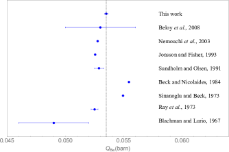
Figure 1: Comparison of the electric quadrupole moment (in barns) of the ⁹Be nucleus obtained using atomic structure calculations.

Conclusions.—

We have determined the electric quadrupole moment $Q_{\rm N}(^{9}{\rm Be})$ with significantly higher accuracy and in disagreement with previous values. The improvement achieved in this work has several independent sources. The first one is the recalculation of the $A_{2}$, $B_{2}$, and $C_{2}$ coefficients from experimental hyperfine splitting. More precisely, including $C_{2}$ in the effective Hamiltonian $H_{\rm hfs,eff}$ in Eq. (13) enabled us to decrease the experimental uncertainties by a factor of 2. The second improvement is due to the inclusion of the hyperfine mixing by exact diagonalization of the effective fine- and hyperfine-structure Hamiltonian of Eq. (Fine and hyperfine structure Hamiltonian.—). The third improvement comes from the very accurate calculation of the expectation values of the fine- and hyperfine-structure operators using explicitly correlated functions allowing for the complete electron correlations. The fourth one is due to the exact inclusion of the finite nuclear mass in the fine and hyperfine interaction in Eqs. (2) and (5). Finally, the fifth source of improvement is due to accounting for the relativistic, radiative and nuclear structure corrections by appropriate rescaling of the $a_{1}$ parameter.

Regarding our theoretical uncertainties, they come exclusively from neglected higher order relativistic and QED contributions, in particular those due to hyperfine mixing of the $2\,^{3}\!P_{1}$ and $2\,^{1}\!P_{1}$ states. The calculation of the complete $\mathcal{O}(\alpha^{2})$ correction is possible but technically difficult. It has been performed for Be⁺ in [Puchalski:14] due to the availability of the exponentially correlated basis functions there. Nevertheless, if a complete $\mathcal{O}(\alpha^{2})$ correction is known, one can use both $B_{1}$ and $B_{2}$ parameters to obtain an even more accurate nuclear quadrupole moment of ⁹Be.

References

- Filin et al. [2020] A. A. Filin, V. Baru, E. Epelbaum, H. Krebs, D. Möller, and P. Reinert, Extraction of the neutron charge radius from a precision calculation of the deuteron structure radius, Phys. Rev. Lett. 124, 082501 (2020). [Puchalski et al.(2020)Puchalski, Komasa, and Pachucki]Puchalski:20M. Puchalski, J. Komasa, and K. Pachucki, Hyperfine structure of the first rotational level in , and HD molecules and the deuteron quadrupole moment, Phys. Rev. Lett. 125, 253001 (2020). [Voelk and Fick(1991)]Voelk:91H.-G. Voelk and D. Fick, The electric moments of 7Li from coulomb scattering, Nucl. Phys. A 530, 475 (1991). [Vinciguerra and Stovall(1969)]Vinciguerra:69D. Vinciguerra and T. Stovall, Electron scattering from p-shell nuclei, Nucl. Phys. A 132, 410 (1969). [Bernheim et al.(1969)Bernheim, Riskalla, Stovall, and Vinciguerra]Bernheim:69M. Bernheim, R. Riskalla, T. Stovall, and D. Vinciguerra, Electron scattering form factor of 9Be, Phys. Lett. B 30, 412 (1969). [Urban and Sadlej(1990)]Urban:90M. Urban and A. J. Sadlej, The nuclear quadrupole moment of Li: Refined calculations of electric field gradients in LiH, LiF, and LiCl, Chem. Phys. Lett. 173, 157 (1990). [Diercksen and Sadlej(1989)]Diercksen:89G. H. Diercksen and A. J. Sadlej, A possible determination of the nuclear quadrupole moment of 9Be from molecular calculations of electric properties of BeH, Chem. Phys. Lett. 155, 127 (1989). [Borin et al.(1992)Borin, Machado, and Ornellas]Borin:92A. C. Borin, F. B. Machado, and F. R. Ornellas, Nuclear motion dependence of the electric field gradient at the 9Be nucleus in BeH+, Chem. Phys. Lett. 196, 417 (1992). [Nemouchi et al.(2003)Nemouchi, Jönsson, Pinard, and Godefroid]Nemouchi:03M. Nemouchi, P. Jönsson, J. Pinard, and M. Godefroid, Theoretical evaluation of the 7,9Be- 4P1/2,3/2,5/2 hyperfine structure parameters and Be 3Po electron affinity, J. Phys. B 36, 2189 (2003). [Tiesinga et al.(2021)Tiesinga, Mohr, Newell, and Taylor]CODATA:18E. Tiesinga, P. J. Mohr, D. B. Newell, and B. N. Taylor, CODATA recommended values of the fundamental physical constants: 2018, Rev. Mod. Phys. (2021), in press. [Krauth et al.(2021)Krauth, Schuhmann, and Ahmed, et al.]Krauth:21J. Krauth, K. Schuhmann, and M. Ahmed, et al., Measuring the -particle charge radius with muonic helium-4 ions, Nature 589, 527 (2021). [Pachucki et al.(2018)Pachucki, Patkós̆, and Yerokhin]Pachucki:18K. Pachucki, V. Patkós̆, and V. A. Yerokhin, Three-photon-exchange nuclear structure correction in hydrogenic systems, Phys. Rev. A 97, 062511 (2018). [Friar and Payne(2005)]Friar:05J. Friar and G. Payne, Deuteron dipole polarizabilities and sum rules, Phys. Rev. C 72 (2005). [Blachman and Lurio(1967)]Blachman:67A. G. Blachman and A. Lurio, Hyperfine structure of the metastable states of and the nuclear electric quadrupole moment, Phys. Rev. 153, 164 (1967). [Beloy et al.(2008)Beloy, Derevianko, and Johnson]Beloy:08K. Beloy, A. Derevianko, and W. R. Johnson, Hyperfine structure of the metastable state of alkaline-earth-metal atoms as an accurate probe of nuclear magnetic octupole moments, Phys. Rev. A 77, 012512 (2008). [Hibbert(1975)]Hibbert:75A. Hibbert, Developments in atomic structure calculations, Rep. Prog. Phys. 38, 1217 (1975). [Eides et al.(2001)Eides, Grotch, and Shelyuto]Eides:01M. I. Eides, H. Grotch, and V. A. Shelyuto, Theory of light hydrogenlike atoms, Phys. Rep. 342, 63 (2001). [Puchalski and Pachucki(2009)]Puchalski:09M. Puchalski and K. Pachucki, Fine and hyperfine splitting of the state in Li and , Phys. Rev. A 79, 032510 (2009). [Kedziorski et al.(2020)Kedziorski, Stanke, and Adamowicz]Kedziorski:20A. Kedziorski, M. Stanke, and L. Adamowicz, Atomic fine-structure calculations performed with a finite-nuclear-mass approach and with all-electron explicitly correlated gaussian functions, Chem. Phys. Lett. 751, 137476 (2020). [Wang et al.(2017)Wang, Audi, Kondev, Huang, Naimi, and Xu]Wang:17M. Wang, G. Audi, F. G. Kondev, W. Huang, S. Naimi, and X. Xu, The AME2016 atomic mass evaluation (II). Tables, graphs and references, Chin. Phys. C 41, 030003 (2017). [Stone(2015)]Stone:15N. J. Stone, Nuclear magnetic dipole and electric quadrupole moments: Their measurement and tabulation as accessible data, J. Phys. Chem. Ref. Data 44, 031215 (2015). [Schwartz(1955)]Schwartz:55C. Schwartz, Theory of hyperfine structure, Phys. Rev. 97, 380 (1955). [Jaccarino et al.(1954)Jaccarino, King, Satten, and Stroke]Jaccarino:54V. Jaccarino, J. G. King, R. A. Satten, and H. H. Stroke, Hyperfine structure of . Nuclear magnetic octupole moment, Phys. Rev. 94, 1798 (1954). [Ray et al.(1973)Ray, Lee, and Das]Ray:73S. N. Ray, T. Lee, and T. P. Das, Study of the nuclear quadrupole interaction in the excited () state of the beryllium atom by many-body perturbation theory, Phys. Rev. A 8, 1748 (1973). [Sinanoǧlu and Beck(1973)]Sinanoglu:73O. Sinanoǧlu and D. R. Beck, HFS constants of Be I 3P0, B I 4P and B I 2D obtained from the non-closed shell many-electron theory for excited states, Chem. Phys. Lett. 20, 221 (1973). [Beck and Nicolaides(1984)]Beck:84D. R. Beck and C. A. Nicolaides, Fine and hyperfine structure of the two lowest bound states of Be- and their first two ionization thresholds, Int. J. Quantum Chem. 26, 467 (1984). [Sundholm and Olsen(1991)]Sundholm:91D. Sundholm and J. Olsen, Large MCHF calculations on the hyperfine structure of Be(3Po): the nuclear quadrupole moment of 9Be, Chem. Phys. Lett. 177, 91 (1991). [Jönsson and Fischer(1993)]Jonsson:93P. Jönsson and C. F. Fischer, Large-scale multiconfiguration Hartree-Fock calculations of hyperfine-interaction constants for low-lying states in beryllium, boron, and carbon, Phys. Rev. A 48, 4113 (1993). [Puchalski and Pachucki(2014)]Puchalski:14M. Puchalski and K. Pachucki, Ground-state hyperfine splitting in the Be+ ion, Phys. Rev. A 89, 032510 (2014). thebibliography