An Abstraction-based Method to Check
Multi-Agent Deep Reinforcement-Learning Behaviors
(Extended Version)

Abstract.

Multi-agent reinforcement learning (RL) often struggles to ensure the safe behaviours of the learning agents, and therefore it is generally not adapted to safety-critical applications. To address this issue, we present a methodology that combines formal verification with (deep) RL algorithms to guarantee the satisfaction of formally-specified safety constraints both in training and testing. The approach we propose expresses the constraints to verify in Probabilistic Computation Tree Logic (PCTL) and builds an abstract representation of the system to reduce the complexity of the verification step. This abstract model allows for model checking techniques to identify a set of abstract policies that meet the safety constraints expressed in PCTL. Then, the agents’ behaviours are restricted according to these safe abstract policies. We provide formal guarantees that by using this method, the actions of the agents always meet the safety constraints, and provide a procedure to generate an abstract model automatically. We empirically evaluate and show the effectiveness of our method in a multi-agent environment.

1. Introduction

Autonomous agents acting in unknown environments are attracting research interests due to their potential applications in multiple domains including robotics, network optimisation, and distributed resource allocation Yang and Gu (2004); Pandey (2016); Zhang et al. (2009); Wiering (2000); Riedmiller et al. (2001). Currently, one of the most popular techniques to tackle these domains is reinforcement learning (RL) Sutton and Barto (2018). However, in order to learn how to act, RL requires to explore the environment, which in safety-critical scenarios means that the agents will commonly take dangerous actions, possibly damaging themselves or even putting humans at risk. Consequently, RL and its extension deep RL (DRL) François-Lavet et al. (2018) are rarely used in real-world applications where multiple safety-critical constraints need to be satisfied simultaneously. To alleviate this problem, (D)RL algorithms are being combined with formal verification techniques to ensure safety in learning. Even though significant progress has been achieved in this direction Mason et al. (2018); Alshiekh et al. (2018); Jansen et al. (2018); Pathak et al. (2018); Garcıa and Fernández (2015); Cheng et al. (2019), settings with multiple learning agents are comparatively less explored and understood.

Our Contribution

In this paper we introduce assured multi-agent reinforcement learning (AMARL), a method to formally guarantee the safe behaviour of agents acting in an unknown environment through the satisfaction of safety constraints by the solution learned using a DRL algorithm, both at training and test time. Building upon the assured reinforcement learning (ARL) technique in Mason et al. (2018), we combine reinforcement learning and formal verification Kwiatkowska (2007) to ensure the satisfaction of constraints expressed in Probabilistic Computation Tree Logic (PCTL) Hansson and Jonsson (1994). Differently from ARL, we support a multi-agent setting and DRL algorithms. Specifically, we introduce the notion of abstract Markov game (AMG) and present a procedure to generate AMGs automatically, unlike ARL where abstract models are handcrafted. Moreover, we provide formal proofs of the preservation of properties expressed in (fragments of) PCTL between the abstract and concrete model.

Multiple challenges arise from multi-agent settings, such as the curse of dimensionality Buşoniu et al. (2010). It is therefore crucial to build a small enough abstract Markov game while preserving all the required properties. Moreover, many RL algorithms cannot guarantee convergence in multi-agents scenarios and are therefore harder to train. Finally, the use of options (i.e., temporally extended actions) in the abstract MG makes the definition of the reward and transition functions complex. Nonetheless, our experimental results demonstrate the effectiveness of the AMARL method to ensure safety constraints. Moreover, we demonstrate its compatibility with DRL algorithms and its ability to ensure the safe behaviours of agents even during the learning stage.

Related Work

This paper builds upon the ARL method introduced in Mason et al. (2018); consequently, both our method and ARL are closely related and belong to the same class of safe RL techniques based on restricting exploration Garcıa and Fernández (2015). Further, they both support constraints expressed in the probabilistic temporal logic PCTL. Nevertheless, our AMARL method is more general than ARL, as we support both multi-agent settings and the use of both tabular RL and DRL. Moreover, in contrast with ARL, the abstract representation of the Markov game is built in an automated manner and proofs of constraint preservation between abstracts and concrete models are provided. Hence, ARL can be seen as a special case of our method, where only single-agent tabular RL is supported and no proof of constraint preservation is provided.

Our approach differs from other safe RL methods based on formal verification, as it relies on the construction of an abstract model to tackle the high dimensional spaces found in typical shield methods Alshiekh et al. (2018); Jansen et al. (2018) and allows to find high-level solutions directly from the abstract model. The approach proposed in Alshiekh et al. (2018) introduced the notion of shield, i.e., an entity that monitors the agents’ actions, and also expresses constraints in temporal logic. A major difference w.r.t. AMARL is that their shield instead of penalizing unsafe actions and preventing the agent from interacting with the environment, replaces the unsafe action with another safe action and therefore requires the shield to be active both at training and test time. Moreover, their method is designed for single-agent RL and constraints are expressed in linear temporal logic Pnueli (1977). Similarly to Alshiekh et al. (2018) and AMARL, Jansen et al. (2018) proposes a shield-based technique that expresses constraints in PCTL. A key difference here is that they consider multi-agent settings where only a single agent is controllable. Their method also relies on the construction of an abstraction. However, differently from AMARL, their abstract model does not include the reward function, thus preventing from solving the problem at the abstract level. The approach presented in Pathak et al. (2018) also expresses safety constraints in PCTL, but instead of ensuring safety by mean of a shield, this method is based on verification and repair of the learned policy. Hence, it does not provide any safety guarantee at learning time. Moreover, a significant limitation of Pathak et al. (2018) is its difficulty to tackle high dimensional state spaces. Thus making this method prone to the curse of dimensionality and not adapted for multi-agent settings that are known to suffer from this problem.

2. Background

In this section, we provide the necessary background regarding both reinforcement learning and formal verification.

2.1. Multi-agent Reinforcement Learning

Multi-agent reinforcement learning (MARL) is a machine learning Bishop (2006) technique where agents situated in an environment aim to maximise an expected reward signal provided by their interactions with such environment Sutton and Barto (2018). This problem is typically modelled as a Markov game (MG). Initially, this model is unknown to the agents and they explore it to collect rewards and to learn the optimal behaviours (i.e., policies).

Definition (Markov Game).

Littman (1994) A Markov game with $n$-agents is a tuple $M=\langle S,A_{1},\ldots,A_{n},$ $P,R_{1},\ldots,R_{n},\gamma\rangle$ where:

• $S$ is the state space.

• For every $i\leq n$, $A_{i}$ is the action space of agent $i$.

• $P$ is the transition function where $P^{\@vec{a}}_{ss^{\prime}}$ denotes the probability of going from state $s\in S$ to state $s^{\prime}\in S$ by taking the joint action $\@vec{a}=\langle a_{1},\ldots,a_{n}\rangle$, where all $a_{i}\in A_{i}$ are the actions taken by the agents simultaneously.

• $R_{1},\ldots,R_{n}$ is a set of reward functions, where $R^{\@vec{\rm a}}_{i,ss^{\prime}}$ denotes the reward received by agent $i$ when the joint action $\@vec{a}$ from state $s\in S$ to state $s^{\prime}\in S$ is performed. We denote $r_{i,t}$ the reward received by agent $i$ at time step $t$.

• $\gamma\in[0,1]$ is the discount factor.

In MARL each agent’s behaviour is determined by her policy. In this work, we use deterministic policies and define the policy of agent $i$ as $\pi_{i}:S\rightarrow A_{i}$. Each agent $i$ tries to find an optimal policy $\pi^{*}_{i}$ that maximises the sum $R_{i}=\sum_{k=0}^{\infty}\gamma^{k}r_{i,t+k}$ of her expected rewards. Finally, a joint policy is a tuple $\@vec{\pi}=\langle\pi_{1},\ldots,\pi_{n}\rangle$.

Moreover, we focus on fully cooperative problems Buşoniu et al. (2010), where all the agents share the same reward function $R_{1}=\ldots=R_{n}$ and try to maximise their common sum of rewards. The method we propose makes use of the popular Independent Q-Learning (IQL) algorithm Tan (1997) due to its simplicity and to the fact that it is the direct extension of the tabular Q-Learning typically used in previous single-agent shielded based approaches Mason et al. (2018); Alshiekh et al. (2018); Jansen et al. (2018). According to IQL, each agent $i$ has her own Q-table and update the values of the state-action pairs as follows:

$$Q_{i,t+1}(s,a_{i})\leftarrow Q_{i,t}(s,a_{i})+\alpha[r_{i,t}+\gamma\cdot\max_{a_{i}^{\prime}\in A_{i}}Q_{i,t}(s^{\prime},a_{i}^{\prime})-Q_{i,t}(s,a_{i})]$$ (1)

where $0<\alpha\leq 1$ is the learning rate. Once the learning phase is over, the optimal policy of an agent using IQL returns the action with the highest Q-value according to the state-action pairs of her Q-table. In this paper, we make use of deep RL, which combines RL and deep learning Goodfellow et al. (2016) to increase the scalability of traditional tabular RL algorithms Mnih et al. (2015). In particular, we use the direct extension of IQL called independent deep Q-Learning (IDQL) Tampuu et al. (2017), where the Q-tables of the agents are replaced by neural networks.

Shield in Safe RL

Our approach makes use of a shield Jansen et al. (2018); Alshiekh et al. (2018); Cheng et al. (2019) to ensure the fulfillment of safety constraints both in training and testing. A shield is an entity that monitors the agents’ actions and prevents them from performing any action that would lead to an unsafe state. Therefore, the shield is generally seen as an intermediate between the agents and the environment that ensure that only safe actions are performed on the environment. Note that it is desired to have a shield that intervenes as little as possible and that does not impact too much the agents’ exploration freedom. Otherwise, the shield could prevent the agents from finding optimal policies. For this reason, it is common to have a shield that penalizes the agents with a negative reward when intervening.

2.2. Formal Verification by Model Checking

The method we propose makes use of the probabilistic computation-tree temporal logic (PCTL) Hansson and Jonsson (1994) to express the constraints to satisfy, possibly extended with rewards Forejt et al. (2011).

We consider a set $AP$ of atomic propositions (or atoms) to label the states of an MG, in order to express that some facts hold at certain states Baier and Katoen (2008).

Definition (PCTL).

Formulae $\Phi$ over a set $AP$ of atoms are built according to the following grammar:

$$\Phi ::= true\mid a\mid\Phi\land\Phi\mid\neg\Phi\mid P_{\sim p}(\varphi)$$

$$\varphi ::= \bigcirc\Phi\mid\Phi U\Phi\mid\Phi U^{\leq n}\Phi$$

where $a\in AP$, $\varphi$ is a path formula, $\sim$ $\in\{<,\leq,>,\geq\}$, $p\in[0,1]$, and $n\in\mathbb{N}$. Intuitively, next $\bigcirc$, until $U$, and bounded until $U^{\leq n}$ are the standard temporal operators; while $P_{\sim p}(\varphi)$ expresses that the path formula $\varphi$ is true with probability $\sim p$.

PCTL formulae are interpreted over the states and paths of a Markov game and $s\models\Phi$ denotes that state formula $\Phi$ holds in state $s$. In particular, for an MG $M$, we introduce a labelling function $L:S\to 2^{AP}$. For reasons of space, we omit the details about the semantics of PCTL and refer to Baier and Katoen (2008); Forejt et al. (2011).

The extended version of PCTL with rewards supported by the PRISM language Kwiatkowska et al. (2011) extends the definition of state formulae with the following clauses Forejt et al. (2011):

$$\Phi::=R_{\sim r}(I^{=k})\mid R_{\sim r}(C^{\leq k})\mid R_{\sim r}(\lozenge\Phi)$$

where $\sim$ $\in\{<,\leq,>,\geq\}$ and $r\in\mathbb{R}_{\geq 0}$.

Intuitively, $R_{\sim r}(I^{=k})$ expresses the reward at time step $k$, $R_{\sim r}(C^{\leq k})$ expresses the expected cumulative reward up to time $k$, and $R_{\sim r}(\lozenge\Phi)$ expresses the expected cumulative reward to reach a state that satisfies $\Phi$.

Finally, we introduce the weak fragment of PCTL (or wPCTL) that discards the next and bounded until operators. That is, path formulae in wPCTL are restricted as follows:

$$\varphi ::= \Phi U\Phi$$

The weak fragment of PCTL features preeminently as the language to express constraint on learning agents, including those stated in Table 1. The Storm model checker Dehnert et al. (2017) supports the same specification language as PRISM, and we use it to verify the satisfaction of such constraints

Table 1. Safety (S) and Optimality (O) Constraints

ID	Constraint	PCTL
$S_{1}$	All agents will be caught with probability $<0.15$.	$P_{<0.15}(\lozenge captured_{all})$
$S_{2}$	Agent $1$ will be caught with probability $<0.15$.	$P_{<0.15}(\lozenge captured_{1})$
$S_{3}$	Agent $i$, $i=2,3$ will be caught with probability $<0.3$.	$P_{<0.3}(\lozenge captured_{i})$
$O_{1}$	All agents will reach the goal area with probability $\geq 0.8$.	$P_{\geq 0.8}(\lozenge goal_{all})$
$O_{2}$	Agent $1$ will reach the goal with probability $\geq 0.85$.	$P_{\geq 0.85}(\lozenge goal_{1})$
$O_{3}$	Agent $i$, $i=2,3$ will reach the goal with probability $\geq 0.8$.	$P_{\geq 0.8}(\lozenge goal_{i})$
$O_{5}$	The expected reward the agents collect collectively is $\geq 7$.	$R_{\geq 7}(\lozenge end_{all})$

3. The Verification of (D)RL Behaviors

In this section we present the main contributions of this work. First, we introduce the motivating example that we use to illustrate the formal machinery as well as for the experimental evaluation in Sec. 4. Then, we provide an overview of our new assured multi-agent RL technique that aims at automatizing and extending to multi-agent settings the ARL method in Mason et al. (2018). In particular, we introduce abstract Markov game (AMG) and define a new notion of bisimulation that guarantees the preservation of formulae in PCTL between an AMG and its corresponding Markov game. Finally, we provide a procedure to generate such AMGs automatically.

3.1. Motivating Scenario: the GFC domain

As motivating scenario we consider the guarded flag-collection domain (GFC) from Mason et al. (2018) that we extend with multiple cooperative agents (Fig. 1).

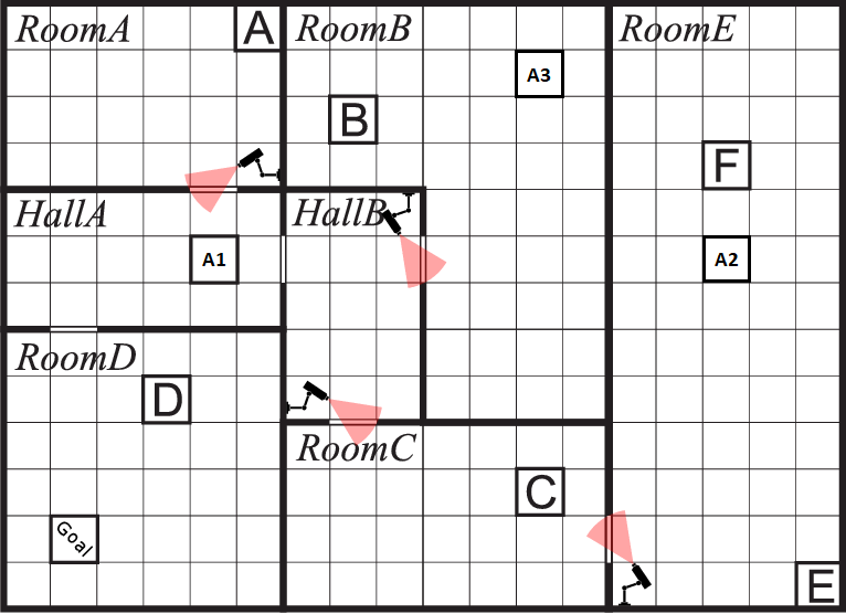
Figure 1. The GFC domain with 3 agents $A_{1}$, $A_{2}$, and $A_{3}$, and 6 flags labelled $A$ to $F$.

Figure showing the Guarded Flag-Collection domain from Mason et al. (2018) that we extended with three agents.

The agents’ objective is to retrieve as many flags as possible without getting caught by the cameras before reaching the Goal position. The detection probability of the cameras is given in Table 2. Agents have a different probability of getting caught depending on the action they perform, i.e., hidden, partial or direct. An agent’s navigation ends when she reaches the goal position or when she gets caught by a camera. An episode terminates when all agents’ navigation is over or when the maximum number of step has been reached.

This scenario illustrates the need to define agent-specific constraints. For instance, we may send multiple robots to collect the flags and some robots might be more valuable than others. Consequently, we want to be able to require the robots to have different probabilities to reach the goal position (see, e.g., Table 1). Further, we observe that the state space grows exponentially with the number of agents: the GFC domain with three agents has $\,\sim 8.2e^{8}$ states versus $\,\sim 1.5e^{4}$ states for the case of a single agent considered in Mason et al. (2018). This remark strengthens the need for our method to be compatible with deep RL algorithms.

Table 2. Detection probabilities of the GFC domain cameras.

	View Detection Probabilities
Area Transitions	Direct	Partial	Hidden
HallA $\leftrightarrow$ RoomA	0.18	0.12	0.06
HallB $\leftrightarrow$ RoomB	0.15	0.1	0.05
HallB $\leftrightarrow$ RoomC	0.15	0.1	0.05
RoomC $\leftrightarrow$ RoomE	0.21	0.14	0.07

3.2. Assured Multi-Agent Reinforcement Learning

The main contribution of this paper is the assured multi-agent reinforcement learning (AMARL) method ensuring formally that teams of autonomous agents satisfy given constraints during the learning process. To this end, we build upon the ARL framework Mason et al. (2018) that we briefly discussed in Sec. 1. In this section, we introduce AMARL by providing an overview of the method, including the different stages it involves. The AMARL pipeline is depicted in Fig. 2.

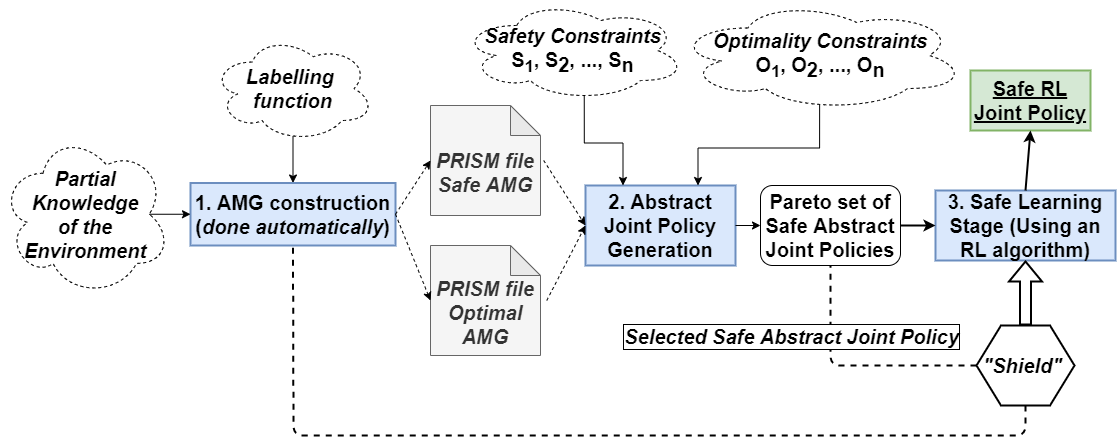
Figure 2. AMARL pipeline, starting with the construction of the abstract MG, then the generation of the abstract joint policies, and terminating with safe learning.

Figure showing the process of the AMARL method. Starting with the AMG construction stage, then with the abstract joint-policy generation stage and terminating with the safe learning stage.

AMG construction

In this stage, the abstract MG corresponding to the given Markov game is generated in an automated manner (see Sec. 3.5). Indeed, only some domain expertise is required to define the labelling function. For instance, in the GFC domain (see Fig. 1), it is sufficient to know the lower and upper bounds detection probabilities of the cameras and the layout of the rooms. Note that since the learning stage makes use of algorithms that are not guaranteed to converge to an optimal solution (such as DRL algorithms), we build both an AMG that considers transitions with the higher chance of reaching a ”bad state” called safe AMG, and an AMG that considers transitions with the lower chance of reaching a ”bad state” called optimal AMG. For instance, in the GFC domain the safe AMG considers the direct transitions in Table 2, whereas the optimal AMG considers hidden transitions. Nonetheless, the two AMGs are identical but for their transition probabilities and, therefore, have the same abstract policies.

Further, we prove a preservation result on the satisfaction of constraints in PCTL between the AMG and the original MG, by using a bisimulation relation Segala and Lynch (1995); Baier and Katoen (2008) (see Sec. 3.4). This is a key difference w.r.t.  ARL, where the abstract model was handcrafted and no preservation guarantees were provided.

Abstract Joint-Policy Generation

In the second stage of AMARL we generate arbitrary joint policies in the AMG. Then, we use the Storm model checker Dehnert et al. (2017) to verify the relevant constraints in PCTL on the AMGs, suitably restricted according to the joint policy. Safety constraints are verified on the safe AMG, whereas optimality constraints on the optimal AMG. (See Table 1 for safety and optimality constraints.) Consequently, the safety constraints allow us to certify that agents always act safely (even during the learning stage, unlike ARL), while the optimality constraints allow us to evaluate the performance of the abstract policies. Finally, as in ARL, we build a Pareto set Liu et al. (2014) of safe abstract joint policies that enables us to choose a Pareto-optimal safe abstract joint policy according to our preferences.

Safe Learning

Finally, even though we obtained the high-level solution, at the concrete level the selected abstract joint policy can be consistent with several different concrete policies. We therefore apply deep RL to let agents learn an optimal concrete policy consistent with the selected safe abstract joint policy. Specifically, we use independent deep Q-Learning Tampuu et al. (2017). Our safe learning stage differs from the corresponding stage of the ARL method on several accounts. Firstly, in order to make our approach compatible with DRL algorithms, we do not remove any action from the action space of the agents. Thus, to make agents learn that some actions are unsafe, we introduce our notion of shield Alshiekh et al. (2018) on the environment as depicted in Fig. 2. Our shield makes use of the AMG to derive the bisimulation relation (See Def. 3.4.1) between the states of the MG and the states of the AMG, then restrict the behaviours of the agents in the original MG to the selected abstract policy. That is, every time an agent selects an action, before letting the agent interacting with the environment, the shield verifies if the agent’s action leads to states allowed by the abstract joint policy and the relaxed bisimulation relation (see Def. 3.4.2). Accordingly, every time the shield block an action, the agent gets a reward of -1 and remains in its current position without interacting with the environment. By doing so, the agent learns that the action is not safe and the shield will no longer be needed at test time when agents follow the learned joint policy. Differently from ARL, to facilitate the learning process of the agents, the shield also recompenses the agents with a reward of 1 every time they complete an option.

3.3. Abstract Markov Games

Due to the general high dimensionality of the problems solved with (deep) RL algorithms, it is typically not possible to apply model checking techniques directly on the concrete problems. A notion of abstraction is therefore required, and it is then necessary to show the class of formulas that can be verified on the abstract model and preserved in the original one. In this section we formally define the notion of abstract Markov game used in the AMARL method. However, we first introduce the concepts of options Sutton et al. (1999) and termination scheme Rohanimanesh and Mahadevan (2003) as they are required for the definition of AMG.

An option is defined as a tuple $o=\langle I_{o},\pi_{o},\beta_{o}\rangle$ where $I_{o}\subseteq S$ is the initialisation set; $\pi_{o}:S\to A$ is its policy; and $\beta_{o}\subseteq S$ is the termination condition Sutton et al. (1999). An option can be thought of as a sequence of actions that once initialised follows a policy until it reaches a termination condition.

When actions are replaced with options, given that options, as sequences of actions, might have different duration and termination condition for different agents, thus terminating at different times, it is required to decide when to terminate the joint option. In this paper, we focus on a fully cooperative setting that uses the $T_{all}$ termination scheme proposed in Rohanimanesh and Mahadevan (2003), whereby the next joint option is decided as soon as all the options currently being executed have terminated. The reason for this choice is that it makes the decision problem synchronous and allows the definition of the reward and transition functions at the abstract level. Moreover, the $T_{all}$ termination scheme is the one that has fewer decision epochs and reduces further the complexity of the problem. Focusing on fully cooperative problems, on the other hand, allows to define the reward function without knowing the particular policy of each agents. For example, in the GFC domain, if two agents try to collect the same flag, it is not necessary to know which agent collects it to define the reward function.

Definition (Abstract Markov Game).

Given a Markov game $M=\langle S,A_{1},\ldots,A_{n},P,R_{1},\ldots,$ $R_{n},$ $\gamma\rangle$, let $O_{1},\ldots,O_{n}$ be a tuple of option spaces over $M$, and $z$ be an abstraction function for $S$. We define the abstract Markov game corresponding to $M$ as a tuple $\bar{M}=\langle\bar{S},O_{1},\ldots,O_{n},\bar{P},\bar{R_{1}},\ldots,$ $\bar{R_{n}},\gamma\rangle$ where:

• $\bar{S}$ is the abstract state space with $z(S)=\bar{S}$.

• For every $i\leq n$, $O_{i}$ is the option space of agent $i$.

• $\bar{P}$ is the transition function where $\bar{P}^{\@vec{\bar{o}}}_{\bar{s}\bar{s^{\prime}}}$ denotes the probability of going from the abstract state $\bar{s}\in\bar{S}$ to the abstract state $\bar{s^{\prime}}\in\bar{S}$ with the joint option $\@vec{o}=\langle o_{1},\ldots,o_{n}\rangle$: $\bar{P}^{\@vec{\bar{o}}}_{\bar{s}\bar{s^{\prime}}}=\sum_{s\in S,z(s)=\bar{s}}w_{s}\sum_{s^{\prime}\in S,z(s^{\prime})=\bar{s^{\prime}}}P(s,\@vec{o},s^{\prime})$

  where $w_{s}$ denotes the weight of state $s$ and represents the degree whereby $s$ contributes to the abstract state $z(s)$ Marthi (2007),

• $\bar{R_{1}},\ldots,\bar{R_{n}}$ is the set of reward function where $\bar{R}^{\@vec{o}}_{i,\bar{s}\bar{s^{\prime}}}$ denotes the reward perceived by agent $i$ when performing the joint option $\@vec{o}=\langle o_{1},\ldots,o_{n}\rangle$ in $M$, from state $\bar{s}\in\bar{S}$ to state $\bar{s^{\prime}}\in\bar{S}$. $\bar{R}^{\@vec{\rm\bar{o}}}_{i,\bar{s}\bar{s^{\prime}}}=\sum_{s\in S,z(s)=\bar{s}}w_{s}R_{i}(s,\@vec{o})$

• $\gamma\in[0,1]$ is the discount factor.

By Def. 3.3 AMGs can be considered as a special case of Markov games where an option is considered as an abstract action and we normally omit the bar above the letters in the notation of AMGs. In Sec. 3.5 we provide an algorithmic way to generate abstract MG so that constraints expressed in wPCTL are preserved, based on the notion of (stutter) bisimulation developed in the following section.

3.4. Stutter Bisimulations

This section is devoted to identifying the conditions under which constraints expressed in PCTL are preserved between an MG and the corresponding abstract MG. To this end, we first consider stutter bisimulations, which are known to preserve the weak fragment of PCTL (wPCTL) in stochastic systems Segala and Lynch (1995). In particular, we provide a new notion of stutter bisimulation adapted for Markov games and prove that this new definition preserves the formulas expressed in wPCTL. Then, as this direct adaptation of stutter bisimulations to Markov games turns out to be too restrictive for the safe learning stage to be efficient, we provide a relaxation of one of the requirements of the stutter bisimulation, thus allowing the agents to learn more independently while reducing the number of interventions of the shield. Finally, we provide a procedure to automatically generate an AMG that is stutter-bisimilar to a given MG.

3.4.1. Stutter Bisimulation

Stutter bisimulations have been introduced for probabilistic systems in Segala and Lynch (1995), where they are referred to as weak bisimulations. Here we extend these bisimulations to Markov games and a multi-agent setting.

We first recall some notations and definitions.

Probability distribution.

For a finite set $X$, a (discrete) probability distribution on $X$ is defined by a function $\mu:X\rightarrow[0,1]$ such that $\sum_{s\in S}\mu(s)=1$. $Dist(X)$ denotes the set of all probability distributions over $X$.

Notation.

Let $S$ be a set of states and $\mathcal{E}$ an equivalence relation over $S$, i.e., a transitive, reflexive and symmetric binary relation on $S$. For each $s\in S$, $[s]_{\mathcal{E}}=\{s^{\prime}\in S\mid(s,s^{\prime})\in\mathcal{E}\}$ denotes the equivalence class of state $s$ under $\mathcal{E}$. Then, $S\backslash\mathcal{E}=\{[s]_{\mathcal{E}}\mid s\in S\}$ is the quotient space of $S$ under $\mathcal{E}$. For a relation $\mathcal{E}$, if ($s_{1},s_{2})\in\mathcal{E}$, we often write $s_{1}\mathcal{E}s_{2}$. Let $M$ be a Markov game, $P(s,\@vec{a},\cdot)$ denotes the discrete probability distribution on $S$ to select the next states, given the current state $s$ and joint action $\@vec{a}$.

Definition ($\mathcal{E}$-equivalence Segala and Lynch (1995)).

Let $\mathcal{E}$ be an equivalence relation over set $S$ and let $\mu_{1},\mu_{2}\in Dist(S)$ be two probability distribution. We say that $\mu_{1}$ and $\mu_{2}$ are $\mathcal{E}$-equivalent, denoted $\mu_{1}\equiv_{\mathcal{E}}\mu_{2}$, iff $\mu_{1}([s]_{\mathcal{E}})=\mu_{2}([s]_{\mathcal{E}})$, for all $[s]_{\mathcal{E}}\in S\backslash\mathcal{E}$, where $\mu([s]_{\mathcal{E}})=\sum_{s^{\prime}\in[s]_{\mathcal{E}}}\mu(s^{\prime})$. That is, $\mu_{1}$ and $\mu_{2}$ are $\mathcal{E}$-equivalent if they assign the same probability weight to every $\mathcal{E}$-equivalence class.

Having recalled the required notations, we now introduce our novel definition of stutter bisimulation specifically for Makov games.

Definition (Stutter Bisimulation).

Let $M_{i}=\langle S_{i},A_{1,i},\ldots,$ $A_{n,i},\allowbreak P_{i},R_{1,i},\ldots,R_{n,i},\gamma_{i}\rangle$, for $i=1,2$, be two Markov games over $AP$ with labelling functions $L_{i}:S_{i}\rightarrow 2^{AP}$ for $M_{1}$ and $M_{2}$. A (stutter) bisimulation for $(M_{1},M_{2})$ is an equivalence relation $\mathcal{E}$ over $S_{1}\cup S_{2}$ such that

1. for every $s_{1}\in S_{1}$, there exists $s_{2}\in S_{2}$ such that $s_{1}\mathcal{E}s_{2}$.

2. for every $s_{2}\in S_{2}$, there exists $s_{1}\in S_{1}$ such that $s_{1}\mathcal{E}s_{2}$.

3. for all $(s_{1},s_{2})\in\mathcal{E}$ it holds that:

   1. $L_{1}(s_{1})=L_{2}(s_{2})$,

   2. for every joint action $\@vec{a}_{1}$ available from state $s_{1}$, there exist a joint option $\@vec{o}_{2}$ available from $s_{2}$ such that $P_{1}(s_{1},\@vec{a}_{1},\cdot)\equiv_{\mathcal{E}}P_{2}(s_{2},\@vec{o}_{2},\cdot)$ and $\@vec{o}_{2}$ respect the branching condition Van Glabbeek and Weijland (1996):

      • for every path $w$ consistent with $\@vec{o}_{2}$ and every state $s$ occurring in $w$, either $s_{1}\mathcal{E}s$ and each state $s^{\prime}$ that precedes $s$ in $w$ satisfies $s_{1}\mathcal{E}s^{\prime}$, or for every $s^{\prime}_{1}\in S_{1}$, $s^{\prime}_{1}\mathcal{E}$ $last(w)$ implies $s^{\prime}_{1}\mathcal{E}s$.

   3. for every joint action $\@vec{a}_{2}$ available from state $s_{2}$, there exist a joint option $\@vec{o}_{1}$ available from $s_{1}$ such that $P_{2}(s_{2},\@vec{a}_{2},\cdot)\equiv_{\mathcal{E}}P_{1}(s_{1},\@vec{o}_{1},\cdot)$ and $\@vec{o}_{1}$ respect the branching condition Van Glabbeek and Weijland (1996):

      • for every path $w$ consistent with $\@vec{o}_{1}$ and every state $s$ occurring in $w$, either $s_{2}\mathcal{E}s$ and each state $s^{\prime}$ that precedes $s$ in $w$ satisfies $s_{2}\mathcal{E}s^{\prime}$, or for every $s^{\prime}_{2}\in S_{2}$, $s^{\prime}_{2}\mathcal{E}$ $last(w)$ implies $s^{\prime}_{2}\mathcal{E}s$.

where $last(w)$ denotes the last state of path $w$.

We write $M_{1}\simeq M_{2}$ whenever there exist a bisimulation $\mathcal{E}$ for $(M_{1},M_{2})$, and for every $(s_{1},s_{2})\in\mathcal{E}$ we write $s_{1}\simeq s_{2}$.

Conditions (1) and (2) in Def. 3.4.1 state that every state of $M_{1}$ is in relation with some state of $M_{2}$ and vice versa. Condition (3.a) requires that bisimilar states are equally labelled. Condition (3.b) says that every outgoing transition $P_{1}(s_{1},\@vec{a}_{1},\cdot)$ must be $\mathcal{E}$-equivalent to some outgoing transition $P_{2}(s_{2},\@vec{o}_{2},\cdot)$. The branching conditions says that for every path $w$ that can occur when following $\@vec{o}_{2}$, all the states in $w$ that appear before the change of equivalence class are related to state $s_{1}$, whereas all the states that appear thereafter are related to the same state $s^{\prime}_{1}\in S_{1}$. Condition (3.c) is the symmetric counterpart to (3.b). As an example, Fig. 3 depicts an MG $M_{1}$ and its corresponding AMG $M_{2}$, which is stutter-bisimilar according to the equivalence relation that induces the following set of equivalence classes $\{\{v_{0},v_{1},v_{2},s_{0}\},$ $\{v_{3},s_{1}\},\{v_{4},s_{2}\}\}$.

Figure 3. The MG $M_{1}$ on the left and its stutter-bisimilar AMG $M_{2}$ on the right.

Figure showing the stutter bisimulation relation on two MGs.

Our definition of stutter bisimulation can be seen as a unified version of the stutter bisimulation for deterministic systems in Baier and Katoen (2008) and the weak bisimulations for probabilistic systems in Segala and Lynch (1995). Indeed, our definition takes into account the state labellings as in Baier and Katoen (2008) and supports the probabilistic case as in Segala and Lynch (1995). However, a notable difference here is the use of options which follow memoryless policies, in contrast with the notions in Baier and Katoen (2008); Segala and Lynch (1995) that use history-based policies. Further, conditions (3.b) and (3.c) in Def. 3.4.1 guarantee that the equivalence relation $\mathcal{E}$ is divergence-sensitive, i.e., the following lemma holds.

Lemma

Let $M_{i}=\langle S_{i},A_{1,i},\ldots,$ $A_{n,i},\allowbreak P_{i},R_{1,i},\ldots,R_{n,i},\gamma_{i}\rangle$, for $i=1,2$, be two bisimilar Markov games, with bisimilar states $s_{1}\in S_{1}$ and $s_{2}\in S_{2}$. For every infinite path $w_{1}$ from $s_{1}$ that always remains in $[s_{1}]_{\mathcal{E}}$, there exists an infinite path $w_{2}$ from $s_{2}$ that always remains in $[s_{2}]_{\mathcal{E}}$ (and viceversa).

Note that we provide in Appendix A all the relevant proofs of the Lemmas and Theorems we introduce in this paper. We now state the main theoretical result in this section about the preservation of wPCTL under stutter bisimulations.

Let $M_{1}$ and $M_{2}$ be two Markov games over $AP$ with labelling functions $L_{i}:S_{i}\rightarrow 2^{AP}$ for $M_{1}$ and $M_{2}$. For every weak PCTL formula $\Phi$, we have that if $M_{1}\simeq M_{2}$, then $M_{1}\models\Phi\iff M_{2}\models\Phi$.

By Theorem 3.4.1 two bisimilar Markov games satisfy the same formulae in wPCTL. This is a key result that allows us to guarantee that, since we can build AMG that are bisimilar to the concrete MG, then all properties expressed in the weak fragment of PCTL that hold in the AMG, also hold in the corresponding MG. However, it is important to note that the branching condition expressed in items (3.b) and (3.c) of Def. 3.4.1 forces agents to coordinate to perform a joint action that transition from a state bisimilar to the initial state of the joint option to a state bisimilar to a terminal state of it, thus preventing from terminating their options independently. As we assume that agents can perform an idle action that does nothing, this condition does not have any impact theoretically. On the other hand, using the shield to guarantee the satisfaction of the branching condition would considerably complicate the learning process and deteriorate the quality of the learned solution. For this reason, in the next section, we introduce a relaxed version of the branching condition that allows agents to terminate their options independently, thus improving the quality of the learned solution and facilitating the learning stage by reducing the number of interventions of the shield, as the agents are normally less likely to violate the constraints for the relaxed version.

3.4.2. Relaxing the Branching Condition

In a multi-agent RL environment it is key to verify the behaviour of each agent independently, e.g., we want to be able to ensure that a specific agent is not reaching a dangerous state. However, some atomic propositions expressing overall goals the agents want to achieve, will be shared by all agents. E.g., in the GFC domain, the flags that have been collected are represented as atoms that are shared amongst all agents as it is a common goal. Following this idea, we denote as $AP_{i}$ the set of atoms whose truth depends only on the local state of agent $i$, such as its position, and $AP_{all}$ the set of atoms whose truth depends on the whole global state of the system. Then, we relax the branching conditions (3.b) and (3.c) in Def. 3.4.1. Note that this relaxed branching condition is only used during the learning stage to define the shield and not during the generation of the abstract model. Thus, the generated abstract model is still stutter bisimilar to the concrete model.

Definition (Relaxed (Stutter) Bisimulation).

Let $M_{i}=\langle S_{i},A_{1,i},\allowbreak\ldots,A_{n,i},P_{i},R_{1,i},\ldots,R_{n,i},\gamma_{i}\rangle$, $i=\{1,2\}$ be two Markov Games over $AP$ with labelling functions $L_{i}:S_{i}\rightarrow 2^{AP}$ for $M_{1}$ and $M_{2}$. A relaxed (stutter) bisimulation for $(M_{1},M_{2})$ is an equivalence relation $\mathcal{E}$ over $S_{1}\cup S_{2}$ such that all conditions in Def. 3.4.1 hold for the following relaxed branching condition:

• for every path $w$ consistent with $\@vec{o}_{k}$ and every state $s$ occurring in $w$,

  1. for each agent $i$, either $L(s)\cap AP_{i}=L(s_{m})\cap AP_{i}$ and each state $s^{\prime}$ that precedes $s$ in $w$ satisfies $L(s^{\prime})\cap AP_{i}=L(s_{m})\cap AP_{i}$, or for every $s^{\prime}_{m}\in S_{m}$, if $L(s^{\prime}_{m})\cap AP_{i}=L(last(w))\cap AP_{i}$ then $L(s^{\prime}_{m})\cap AP_{i}=L(s)\cap AP_{i}$

  2. either $L(s)\cap AP_{all}=L(s_{m})\cap AP_{all}$ and each state $s^{\prime}$ that precedes $s$ in $w$ satisfies $L(s^{\prime})\cap AP_{all}=L(s_{m})\cap AP_{all}$, or for every $s^{\prime}_{m}\in S_{m}$, if $L(s^{\prime}_{m})\cap AP_{all}=L(last(w))\cap AP_{all}$ then $L(s^{\prime}_{m})\cap AP_{all}=L(s)\cap AP_{all}$.

where $last(w)$ denotes the last state of path $w$, $k,m\in\{1,2\},k\neq m$.

We write $M_{1}\simeq_{r}M_{2}$ whenever there exist a relaxed bisimulation $R$ for $(M_{1},M_{2})$, and for $(s_{1},s_{2})\in\mathcal{E}$, we write $s_{1}\simeq_{r}s_{2}$.

Intuitively, the difference between the relaxed condition in Def. 3.4.2 and items (3.b) and (3.c) in Def. 3.4.1 is that, instead of ensuring that between the initial and the last state of a path all atoms either change simultaneously or do not change, only ensures that the atoms in each $AP_{i}$, either change at the same time or do not change, with the atoms belonging to set $AP_{all}$ considered independently.

We now state the following theorem, which adapts Theorem 3.4.1 to formulae containing atoms of a single agent, as well as formulae with no restriction on the atoms. Let $M_{1}$ and $M_{2}$ be two Markov games over $AP$ with labelling functions $L_{i}:S_{i}\rightarrow 2^{AP}$ for $M_{1}$ and $M_{2}$.

1. For every wPCTL formula $\Phi$ that only contains atoms in $AP_{i}$ we have that if $M_{1}\simeq_{r}M_{2}$, then $M_{1}\models\Phi\iff M_{2}\models\Phi$.

2. For every wPCTL formula $\Phi$ where path formulae are restricted to $(true$ $U$ $\Phi)$ and $(false$ $U$ $\Phi)$, i.e., $\lozenge\Phi$ and $\Phi$, we have that if $M_{1}\simeq_{r}M_{2}$, then $M_{1}\models\Phi\iff M_{2}\models\Phi$. Moreover, assuming that $\Phi$ only contains one atom and no restriction on path formulae, if $M_{1}\simeq_{r}M_{2}$, then $M_{1}\models\Phi\iff M_{2}\models\Phi$.

We, therefore, defined a relaxation for the branching condition of bisimulation that allows to construct more easily the shield in the safe learning stage. However, it is worth to mention that even though the shield can enable agents to perform actions that lead to a state that is neither bisimilar to the initial state nor to a terminal state of the joint option in the sense of Def. 3.4.1, still it has to verify that after performing an action the global probability of reaching the target equivalence classes remains the same.

Thus, as mentioned in Sec, 3.2, our shield is built according to the relaxed version of the branching condition and by Theorem 3.4.2, it ensures the preservation of some wPCTL formulae both during the learning stage and by the learned solution.

3.5. Building Bisimilar Abstract Markov Games

In this section we provide an algorithm to construct the abstract MG corresponding to a given Markov game, so that the AMG is stutter bisimilar to the original MG.

As the starting point, we consider the algorithm given in Baier and Katoen (2008) to compute the quotient transition system under stutter bisimulation for deterministic systems, which is based on the partition refinement technique Kwiatkowska and Parker (2012). We, therefore, adapt this algorithm to compute AMGs under stutter bisimulation. Throughout this section, let $M=\langle S,A_{1},\ldots,A_{n},P,R_{1},$ $\ldots,R_{n}\gamma\rangle$ be a Markov game over AP with labelling function $L:S\rightarrow 2^{AP}$. Moreover, the abstraction function $z$ we introduced in Def. 3.3 maps each state $s$ to its equivalence class according to the interpretation of atoms.

Definition (Splitter).

Let $\Pi$ be a partition of $S$ and let $B\in\Pi$, we have that:

1. A transition $P(s,\@vec{a},\cdot)$, for $s\in B$, $\@vec{a}=\langle a_{1},\ldots,a_{n}\rangle$, $a_{i}\in A_{i}$ is a $\Pi$-$splitter$ for $B$ iff there exists a state $s^{\prime}\in B$ that does not have any joint option respecting the branching condition that matches $P(s,\@vec{a},C)$ for every $C\in\Pi$.

2. $\Pi$ is $B$-$stable$ if there is no $\Pi$-$splitter$ for $B\in\Pi$.

3. $\Pi$ is $stable$ if $\Pi$ is $B$-$stable$ for all blocks $B\in\Pi$.

In words, $P(s,\@vec{a},\cdot)$ is a $\Pi$-$splitter$ for $B$ if it violates conditions (3.b) and (3.c) in Def. 3.4.1, i.e., there exist a state $s^{\prime}\in B$ from where there exist no joint option respecting the branching condition that can mimic the transition $P(s,\@vec{a},\cdot)$. Given that the initial partition obtained with the abstraction function $z$ groups the states in blocks that share the same labelling of atoms, it is easy to see that if $\Pi$ is stable, then $\Pi$ is a stutter bisimulation.

Once introduced the notion of splitter, we show how to split a block $B\in\Pi$ according to a transition $P(s,\@vec{a},\cdot)$ that was identified as a $\Pi$-$splitter$ of $B$. Thus, we define the function $Split(B,P(s,\@vec{a},\cdot))$ = $\{B\cap Sat_{B}(P(s,\@vec{a},\cdot)),B\backslash Sat_{B}(P(s,\@vec{a},\cdot))\}$, where $Sat_{B}(P(s,\@vec{a},\cdot))$ denotes the set of states in $B$ that have a joint option respecting the branching condition that can mimic transition $P(s,\@vec{a},\cdot)$. We can now define the function $Refine(\Pi,B,\delta)$ that refines a partition $\Pi$.

Definition (Refinement).

Let $\Pi$ be a partition for state space $S$, $B\in\Pi$, and $P(s,\@vec{a},\cdot)$ a $\Pi$-$splitter$ of $B$. Then,

$Refine(\Pi,B,P(s,\@vec{a},\cdot))$ = $Split(B,P(s,\@vec{a},\cdot))\cup(\Pi\backslash B)$

By using Def. 3.5, we present in Algorithm 1 the refinement procedure for quotienting Markov games according to our stutter bisimulation, which is an adaptation of the algorithm for stutter bisimulation quotienting in Baier and Katoen (2008).

Note that we are only interested in the generation of stutter bisimulation and not in relaxed stutter bisimulation as the definition of the relaxed stutter bisimulation is based on a relation that is a stutter bisimulation. The relaxed stutter bisimulation is less strict than the stutter bisimulation, thus if we have a relation that is a stutter bisimulation, this relation also fullfil the conditions of the relaxed stutter bisimulation. The only difference is that the relaxed stutter bisimulation allows to reach the next abstract state by going through some abstract states that are not in relation with the initial one nor the final one. From an AMG that is a stutter bisimulation, it is easy to build a shield that restrict the actions of the agents according to the relaxed version of the branching condition.

input : An MG $M$ without terminal states over $AP$ and its corresponding labeling function $L$

output : Stutter bisimulation quotient space $S/\simeq$

$\Pi:=\Pi_{AP}$ ;

  $\backslash\backslash$ $\Pi_{AP}$ is the initial partition that aggregate states with the same atoms. An algorithm to compute $\Pi_{AP}$ is provided in Baier and Katoen (2008).

while $\exists B\in\Pi,\exists P(s,a,\cdot),s\in B.$ such that $P(s,a,\cdot)$ is a $\Pi$-$splitter$ for $B$ do

       choose such $B\in\Pi,P(s,a,\cdot),s\in B$

       $\Pi:=Refine(\Pi,B,P(s,a,\cdot))$

return $\Pi$

Algorithm 1 Algorithm to compute the stutter bisimulation quotient

4. Experimental Evaluation

We evaluate empirically the performance of our method on the GFC domain with three agents presented in Sec. 3.1, against the safety and optimality constraints in Table 1. All our experiments are run using an Nvidia Tesla (12GB RAM) - 24-core/48 thread Intel Xeon CPU with 256GB RAM. The DRL algorithm we use is IDQL Tampuu et al. (2017) with Double Deep Q-Learning Van Hasselt et al. (2016) and the Dueling Network Architecture Wang et al. (2016). We refer to Appendix B for the details on hyperparameters. Each final policy evaluation is repeated $1e^{4}$ times.

For our experiments, the fully cooperative reward function of the AMGs is defined as follows: a reward of 1 is obtained for each flag collected and for each agent that reaches the goal position of the environment. It is important to realise that the reward function of the AMGs is not used for training purpose but only for evaluating the score of the abstract joint policies and thus to verify if an abstract joint policy meets the optimality constraints expressed on the rewards obtained. In fact, the reward function of the concrete MG is defined as follows:

Definition .

Each agent gets an individual reward of 1 upon collecting a flag and for reaching the goal area of the environment.

Moreover, the shield assigns a reward of 1 to each agent that completes an option and a -1 penalty to each agent that tries to perform an unsafe action, i.e. an action not allowed by the selected abstract joint policy. Note that we do not penalise an agent that gets caught as she is already naturally penalised by the fact that she cannot navigate the environment and get rewards anymore. Thus, even though agents have the common objective of collecting as many flags as possible before reaching the goal area of the environment, to facilitate the learning stage, they have different reward functions at the concrete level. This difference of reward function between the AMGs and the concrete MG does not impact the properties preservation as the score of the abstract joint policy is evaluated according to the atoms of the states it reaches.

To evaluate AMARL, we first run the AMG construction stage to obtain the safe and optimal AMGs. In the second stage, we generate 1,000 abstract joint policies and verify our constraints on them by using the Storm model checker Dehnert et al. (2017). Given the large number of state of our problem and the fact that the number of possible abstract joint policies increases exponentially with the number of states, it is difficult to find a policy that satisfies the expressed constraints. In the current setting, we only obtain one abstract joint policy that meets the constraints (see Table 3). Finally, we run the safe learning stage of our method and obtain the results presented in Table 4. Note that at test time, the shield of our method is no longer active and agents follow their learned policies in a traditional way and that during training agents always meet the safety constraints thanks to the shield. From results in Table 4, we see that the learned policies satisfy the safety constraints as well as the optimality constraints defined in Table 1. Additionally, the constraints satisfied by the learned policies closely match the results returned by Storm meaning that the agents learned polices just marginally worse than optimal. This small divergence is potentially caused by scenarios where one or more agents get captured which were not frequent enough during the training stage for the remaining agents to learn the selected abstract joint policy.

Table 3. Abstract joint policy’s properties returned by Storm that satisfy the constraints. $P_{?}(\Phi)$ denotes the probability of reaching a state that satisfies $\Phi$, while $R_{?}(\Phi)$ denotes the expected reward obtained by reaching such a state.

Optimality properties
$\bm{P_{?}(\lozenge goal_{all})}$	$\bm{P_{?}(\lozenge goal_{1})}$	$\bm{P_{?}(\lozenge goal_{2})}$	$\bm{P_{?}(\lozenge goal_{3})}$	$\bm{R_{?}(\lozenge end_{all})}$
0.8393	1	0.8835	0.9422	7.8007

Safety properties
$\bm{P_{?}(\lozenge captured_{all})}$	$\bm{P_{?}(\lozenge captured_{1})}$	$\bm{P_{?}(\lozenge captured_{2})}$	$\bm{P_{?}(\lozenge captured_{3})}$
0	0	0.297	0.176

Table 4. AMARL test performance applying IDQL on the abstract joint policy from Table 3. Results are presented as the mean and standard deviation from 5 independent runs.

$\bm{i}$	$\bm{P_{?}(\lozenge captured_{i})}$	$\bm{P_{?}(\lozenge goal_{i})}$	$\bm{R_{?}(\lozenge end_{i})}$
$\bm{1}$	0.0 (0.0)	0.9859 (0.271)	1.9859 (0.0271)
$\bm{2}$	0.1184 (0.0033)	0.8733 (0.0195)	3.8022 (0.022)
$\bm{3}$	0.0523 (0.0029)	0.8739 (0.0189)	1.9111 (0.0297)
$\bm{all}$	0.0 (0.0)	0.8379 (0.0023)	7.6992 (0.0553)

In order to fairly evaluate the impact the shield has, we run a second experiment without the use of this element, whereby an episode terminates as soon as some agent reaches an unsafe state (i.e., a state that violates the joint abstract policy) and the agent that performed the unsafe action is penalised with a reward of -1. Further, to make the comparison as fair as possible, we keep the same reward function as before (See Def. 4) where additionally, agents are given a reward of 1 when completing an option and their interactions with the environment are restricted until the termination of the joint option so that we keep the $T_{all}$ termination scheme.

The performance of the solutions learned in this experiment are provided in Table 5. Contrasting these results with the ones in Table 4 we see that the use of the shield has no negative impact on the final performance of the agents. Nevertheless, when learning without the shield the agents reach an unsafe state in 61% of the episodes over the 5 independent runs, while in the shield-based approach safety is always guaranteed. Finally, we also compared our method with a vanilla IDQL approach that does not take advantage of the abstraction. We observe that, in this case, the agents do not converge to an optimal solution in addition to their unsafe behaviours. We refer to Appendix C for details on this experiment.

Table 5. AMARL test performance after being trained without the shield on the abstract joint policy from Table 3. Results are presented as in Table 4.

$\bm{i}$	$\bm{P_{?}(\lozenge captured_{i})}$	$\bm{P_{?}(\lozenge goal_{i})}$	$\bm{R_{?}(\lozenge end_{i})}$
$\bm{1}$	0.0 (0.0)	0.9192 (0.0297)	1.9044 (0.0522)
$\bm{2}$	0.1264 (0.0258)	0.8375 (0.0316)	3.7555 (0.0565)
$\bm{3}$	0.0529 (0.0043)	0.8553 (0.0414)	1.8902 (0.0334)
$\bm{all}$	0.0 (0.0)	0.8293 (0.0242)	7.5501 (0.0716)

5. Conclusion And Future Work

In this paper we put forward a methodology to formally guarantee that solutions learned using deep RL algorithms in a multi-agents setting satisfy specific constraints, even during the learning stage. By taking as starting point the ARL method proposed in Mason et al. (2018), we defined the notion of abstract Markov game meant to reduce the complexity of the original problem, modelled as a Markov game. The construction of the AMG allows to increase the scalability of the verification method by applying model checking techniques on the abstract model. We also defined a notion of stutter bisimulation for MGs, which we proved to be adapt to preserve the weak fragment of PCTL. We thus established the conditions an AMG has to satisfy to guarantee that true properties, expressed in wPCTL, are preserved in the corresponding MG.

Furthermore, in order to keep the learning stage efficient, we defined a relaxation of stutter bisimulation to allow agents to act as independently as possible. Accordingly, we introduced the classes of wPCTL formulae that are preserved when the learning stage takes advantage of this relaxation. Therefore, we provided formal guarantees of property preservation between an AMG and its corresponding MG. This contribution, unlike the ARL method, allows us to ensure the safe behaviours of agents both at training and testing time. Moreover, we provided an algorithm to generate the bisimilar AMG automatically. Finally, our AMARL method allows for choosing beforehand the policy to be learnt among a set of safe solutions, thus permitting to select the most adapted solution for the problem regarding both safety and optimality, depending on the application at hand.

The empirical evaluation we ran on the GFC domain showed that the safety constraints were always satisfied, and that the solution learned using DRL almost always converged to the optimal solution with respect to the selected abstract joint policy, and that it improves on the solution found using the same DRL algorithm without AMARL. The experiments also showed that in addition to ensuring agents safety, the shield of our method had no negative impact and even improved by a bit the agents’ final performance in comparison to AMARL without the shield.

Future work on the AMARL method would include increasing its scalability, also through a more efficient implementation of the procedure to automatically generate the abstract MG. A natural continuation of this work would deal with different termination scheme, as well as support competitive and mixed games. Finally, a further work is needed to apply AMARL to a wider range of problems as well as a broader class of PCTL contraints.

Appendix A Proofs of Theorems and Lemmas

In order to prove our Lemmas and Theorems, we are first required to introduce the following notations.

Notation

For infinite path fragments $w_{i}=s_{0,i}s_{1,i}s_{2,i}...,i=1,2$, we say that $w_{1}$ and $w_{2}$ are bisimilar, denoted $w_{1}\simeq w_{2}$, iff both paths can be divided into segments $s_{j_{r},1}s_{j_{r}+1,1}s_{j_{r}+2,1}...s_{j_{r+1},1}$ and $s_{k_{r},2}s_{k_{r}+1,2}s_{k_{r}+2,2}$ $...s_{k_{r+1},2}$ respectively with $r=1,2,3...$, $0=j_{0}<j_{1}<j_{2}<...$, $0=k_{0}<k_{1}<k_{2}<...$ and that are statewise bisimilar.

Similarly, we sat that $w_{1}$ and $w_{2}$ are partially bisimilar, denoted $w_{1}\simeq_{r}w_{2}$, iff both paths can be divided into segments $s_{j_{r},1}s_{j_{r}+1,1}$ $s_{j_{r}+2,1}$ $...s_{j_{r+1},1}$ and $s_{k_{r},2}s_{k_{r}+1,2}s_{k_{r}+2,2}...s_{k_{r+1},2}$ respectively with $r=1,2,3...$, $0=j_{0}<j_{1}<j_{2}<...$, $0=k_{0}<k_{1}<k_{2}<...$, where for every $r$, $s_{j_{r},1}\simeq_{r}s_{k_{r},2}$ and every state between $s_{j_{r},1}$ and $s_{j_{r+1},1}$ and between $s_{k_{r},1}$ and $s_{j_{k+1},1}$, respect the relaxed branching condition.

A.1. Proof of Lemma 3.4.1 and Theorem 3.4.1

The proof of Theorem 3.4.1 is done by induction over the structure of $\Phi$ similarly to what is done in Baier and Katoen (2008) for the proof of preservation properties of stutter bisimulation for deterministic systems. However, we first need to introduce the following definition and lemma.

Definition .

Let $M_{1}$ and $M_{2}$ be two Markov games. For each $w\in Paths(M)$, $[w]_{\simeq}$ denotes the equivalence class of path $w$, i.e., $[w]_{\simeq}=\{w^{\prime}\in Paths(M)\mid w\simeq w^{\prime}\}$. $Paths(M)$ denotes the set of all paths available in $M$, i.e. $Paths(M)=\bigcup_{s\in S}Paths(s)$ where $Paths(s)$ denotes the set of all paths available from $s$. We write $P_{\pi}([w]_{\simeq})=\sum_{w\in[w]_{\simeq}}P_{\pi}(w)$ to denotes the probability that a path $w\in[w]_{\simeq}$ occurs when following the policy $\pi$. We write $W/M$ to denotes the set consisting of all equivalence classes of path of $M$.

Lemma

Let $M_{1}$ and $M_{2}$ be two Markov games over $AP$ with labelling functions $L_{i}:S_{i}\rightarrow 2^{AP}$ for $M_{1}$ and $M_{2}$. Given $s_{1}\in S_{1}$ and $s_{2}\in S_{2}$, if $s_{1}\simeq s_{2}$, then:

• For all $\pi_{1},w_{1}$ such that $P_{\pi_{1}}([w_{1}]_{\simeq})>0$, there exists $\pi_{2},w_{2}$ such that $w_{1}\simeq w_{2}$ and $P_{\pi_{1}}([w_{1}]_{\simeq})=P_{\pi_{2}}([w_{2}]_{\simeq})$.

• For all $\pi_{2},w_{2}$ such that $P_{\pi_{2}}([w_{2}]_{\simeq})>0$, there exists $\pi_{1},w_{1}$ such that $w_{1}\simeq w_{2}$ and $P_{\pi_{1}}([w_{1}]_{\simeq})=P_{\pi_{2}}([w_{2}]_{\simeq})$.

where $w_{1}\in Paths(s_{1})$ and $w_{2}\in Paths(w_{2})$.

In words, the first item states that for every policy $\pi_{1}$ and every path $w_{1}$ that belongs to the set of all possible paths that start in $s_{1}$ and that can occur when following the policy $\pi_{1}$, there exist a policy $\pi_{2}$ and a path $w_{2}$ such that $w_{1}\simeq w_{2}$ and the probability that a bisimilar path of $w_{1}$ in $M_{1}$ occurs is equal to the probability that a bisimilar path of $w_{2}$ in $M_{2}$ occurs. The second item is its symmetric counterpart.

Notice that Lemma 3.4.1 is a special case of Lemma A.1 where the possible policies are restricted to policies that always remain in the same equivalence class. Therefore, by proving Lemma A.1, we also prove Lemma 3.4.1.

Proof.

The proof of the first statement of Lemma A.1 directly follows from our definition of bisimulation and is done by induction. The proof of the second statement is omitted as by symmetry, is similar.

Induction basis.

The induction basis (i=0) is straightforward as it only consists of the first state of the path. By definition we have that $s_{0,1}\simeq s_{0,2}$ and therefore for the path fragment $w_{1}=s_{0,1}$ we have a path fragment $w_{2}=s_{0,2}$ with both probability 1.

Induction step.

Assume $i\geq 0$ and that the path fragments:

$$\begin{split}w_{1}&=s_{0,1}s_{1,1}s_{2,1}...s_{i,1}(1)\\ w_{2}&=s_{0,2}u_{0,0}...u_{0,n_{0}}s_{1,2}u_{1,0}...u_{1,n_{1}}s_{2,2}...s_{i,2}(2)\end{split}$$

are already constructed and that $P_{\pi_{1}}([w_{1}]_{\simeq})=P_{\pi_{2}}([w_{2}]_{\simeq})$

According to the definition of bisimulation, since $s_{i,1}\simeq s_{i,2}$, for every possible transition from $s_{i,1}$ to some states $s_{i+1,1}$ following $\pi_{1}$, there exists $k\geq 1$ finite path fragments of the form $s_{i,2},u_{i,0}...u_{i,n_{i}}s_{i+1,2}$ following $\pi_{2}$ such that:

$$s_{i+1,1}\simeq s_{i+1,2},s_{i,2}\simeq u_{i,0}\simeq...\simeq u_{i,n_{i}}$$

and for each possible $s_{i+1,1}$, the probability of reaching each equivalence class $[s_{i+1,1}]_{\mathcal{E}}$ from $s_{i,1}$, denoted $P_{\pi_{1}}(s_{i,1},[s_{i+1,1}]_{\mathcal{E}})$, is equal to the probability of reaching each equivalence class $[s_{i+1,2}]_{\mathcal{E}}$ from $s_{i,2}$, denoted $P_{\pi_{2}}(s_{i21},[s_{i+1,2}]_{\mathcal{E}})$. By appending each possible state $s_{i+1,1}$ to the path (1) and each path fragments $s_{i,2},u_{i,0}...u_{i,n_{i}}s_{i+1,2}$ to the path (2), we obtain a set of paths that meet the desired conditions, i.e., each paths resulting of the concatenation of (1) and states $s_{i+1_{1}}$ that belongs to the same equivalence class, will be bisimilar by definition and each paths resulting of the concatenation of (2) and each path fragments $s_{i,2},u_{i,0}...u_{i,n_{i}}s_{i+1,2}$ with $s_{i+1,2}$ that belongs to the same equivalence class, will also be bisimilar. Thus, for each $w^{\prime}_{1}$ resulting from the concatenation with (1), we have that $P_{\pi_{1}}([w^{\prime}_{1}]_{\simeq})=P_{\pi_{1}}([w_{1}]_{\simeq})\cdot P_{\pi_{1}}(s_{i,1},[s_{i+1,1}]_{\mathcal{E}})$ and for each $w^{\prime}_{2}$ resulting from the concatenation with (2), we have that $P_{\pi_{2}}([w^{\prime}_{2}]_{\simeq})=P_{\pi_{2}}([w_{2}]_{\simeq})\cdot P_{\pi_{2}}(s_{i,2},[s_{i+1,2}]_{\mathcal{E}})$, thus for each $w^{\prime}_{1}$ there exist a $w^{\prime}_{2}$ such that $w^{\prime}_{1}\simeq w^{\prime}_{2}$ and therefore $P_{\pi_{1}}([w^{\prime}_{1}]_{\simeq})=P_{\pi_{2}}([w^{\prime}_{2}]_{\simeq})$. ∎

We now provide proof of Theorem 3.4.1.

Proof.

Let $M_{1}\simeq M_{2}$ and let $\mathcal{E}\subseteq S_{1}\cup S_{2}$ be the equivalence relation between them. Let $s_{1}\in S_{1},s_{2}\in S_{2}$ and $w_{1}\in Paths(M_{1}),w_{2}\in Paths(M_{2})$. We have:

1. If $s_{1}\simeq s_{2}$ according to $\mathcal{E}$, then for any wPCTL formula $\Phi$: $s_{1}\models\Phi\iff s_{2}\models\Phi$.

2. If $w_{1}\simeq w_{2}$, then for any wPCTL path formula $\varphi$: $w_{1}\models\varphi\iff w_{2}\models\varphi$.

Induction basis.

Let $s_{1}\simeq s_{2}$. For $\Phi=true$, proposition (1) clearly holds. Given that $L_{1}(s_{1})=L_{2}(s_{2})$, we have that for $\Phi=a\in AP$:

$s_{1}\models a\iff a\in L_{1}(s_{1})\iff a\in L_{2}(s_{2})\iff s_{2}\models a$.

Induction step.

Assume $\Phi_{1},\Phi_{2},\Phi_{3},\Phi_{4}$ are wPCTL state formulae for which proposition (1) holds. Let $s_{1}\simeq s_{2}$.

Case 1: $\Phi=\Phi_{1}\land\Phi_{2}$. The application of the induction hypothesis for $\Phi_{1}$ and $\Phi_{2}$ gives:

$$\begin{split}s_{1}\models\Phi_{1}\land\Phi_{2}&\iff s_{1}\models\Phi_{1}\text{ and }s_{1}\models\Phi_{2}\\ &\iff s_{2}\models\Phi_{1}\text{ and }s_{2}\models\Phi_{2}\\ &\iff s_{2}\models\Phi_{1}\land\Phi_{2}.\\ \end{split}$$

Case 2: $\Phi=\neg\Phi_{3}$. The application of the induction hypothesis for $\Phi_{3}$ gives:

$$\begin{split}s_{1}\models\neg\Phi_{3}&\iff s_{1}\not\models\Phi_{3}\\ &\iff s_{2}\not\models\Phi_{3}\\ &\iff s_{2}\models\neg\Phi_{3}.\\ \end{split}$$

Case 3: $\Phi=P_{\sim p}(\varphi)$. We only prove the case where $\Phi=P_{\geq p}(\varphi)$ as the other cases are similar to this one. We first prove by contraposition that $s_{1}\models\Phi\implies s_{2}\models\Phi$: Assume that $s_{2}\not\models\Phi$. According to the satisfaction relation of wPCTL, we have that if $s_{2}\not\models\Phi$, it means that there exists a policy $\pi_{2}$ of $M_{2}$ such that:

$$\sum_{[w_{2}]_{\simeq}\in W/M_{2},w_{2}\in Paths(s_{2}),w_{2}\models\varphi}P_{\pi_{2}}([w_{2}]_{\simeq})<p$$

and therefore for this policy $\pi_{2}$, there exists a policy $\pi_{1}$ such that for every $w_{2}\in Paths(s_{2})$ there exist a $w_{1}\in Paths(s_{1})$ such that $P_{\pi_{2}}([w_{2}]_{\simeq})=P_{\pi_{1}}([w_{1}]_{\simeq})$ and $w_{1}\simeq w_{2}$ by Lemma A.1. From the induction hypothesis (2) it follows that if $w_{1}\simeq w_{2}$, $w_{2}\models\varphi\iff w_{1}\models\varphi$ and therefore according to lemma A.1, if $s_{2}\not\models\Phi$, then $s_{1}\not\models\Phi$. Thus we proved that $s_{2}\not\models\Phi\implies s_{1}\not\models\Phi$, that is, $s_{1}\models\Phi\implies s_{2}\models\Phi$ by contraposition. It remains to prove that $s_{2}\models\Phi\implies s_{1}\models\Phi$ but we omit the details for symmetry reason.

Case 4: $\Phi=R_{\sim r}(\lozenge\Phi_{4})$. The proof for this case is similar to the proof of Case 3, and we, therefore, omit the details for simplicity. The only non-trivial part of the proof for this case is that is is necessary to notice that $\lozenge\Phi_{4}$ is equal to the path formulae $\varphi=true$ $U$ $\Phi_{4}$ and thus from the induction hypothesis (2) it follows that if $w_{1}\simeq w_{2}$, $w_{2}\models\varphi\iff w_{1}\models\varphi$.

We now prove statement (2). Assume claim (1) holds for wPCTL state formulae $\Phi_{1}$ and $\Phi_{2}$. Let $w_{1}\simeq w_{2}$. We write $w_{i}[...j]$ to denotes the prefix $s_{0,i}s_{1,i}s_{2,i}...s_{j-1,i}$ of $w_{i}$. The only case we need to prove for wPCTL path formula is the case where $\varphi=\Phi_{1}U\Phi_{2}$.

The induction hypothesis for $\Phi_{1}$ and $\Phi_{2}$ and the path fragments $w_{i},i=1,2$ gives:

$w_{1}\models\Phi_{1}U\Phi_{2}$	$\iff$	there exists an index $j_{r}\in\mathbb{N}$ with
		$w_{1}[j_{r}]\models\Phi_{2}$ and
		$w_{1}[...j_{r}]\models\Phi_{1}$
	$\iff$	there exists ans index $k_{r}\in\mathbb{N}$ with
		$w_{2}[k_{r}]\models\Phi_{2}$ and
		$w_{2}[...k_{r}]\models\Phi_{1}$
	$\iff$	$w_{2}\models\Phi_{1}U\Phi_{2}$

where $r\in\mathbb{N}^{*}$. The above clearly hold by definition of the stutter bisimulation. ∎

A.2. Proof of Theorem 3.4.2

The proof of Theorem 3.4.2 of our paper is similar to the proof of Theorem 3.4.1 but for some details. We thus adapt Definition. A.1 and Lemma A.1 for the relaxed version of bisimulation.

Definition .

Let $M_{1}$ and $M_{2}$ be two Markov games. For each $w\in Paths(M)$, $[w]_{\simeq_{r}}$ denotes the partial equivalence class of path $w$, i.e., $[w]_{\simeq_{r}}=\{w^{\prime}\in Paths(M)\mid w\simeq_{r}w^{\prime}\}$. We write $P_{\pi}([w]_{\simeq_{r}})=\sum_{w\in[w]_{\simeq_{r}}}P_{\pi}(w)$ to denotes the probability that a path $w\in[w]_{\simeq_{r}}$ occurs when following the policy $\pi$. We write $W_{r}/M$ to denotes the set consisting of all partial equivalence classes of path of $M$.

Lemma

Let $M_{1}$ and $M_{2}$ be two Markov games over $AP$ with labelling functions $L_{i}:S_{i}\rightarrow 2^{AP}$ for $M_{1}$ and $M_{2}$. Given $s_{1}\in S_{1}$ and $s_{2}\in S_{2}$, if $s_{1}\simeq_{r}s_{2}$, then:

• For all $\pi_{1},w_{1}$ such that $P_{\pi_{1}}([w_{1}]_{\simeq_{r}})>0$, there exists $\pi_{2},w_{2}$ such that $w_{1}\simeq_{r}w_{2}$ and $P_{\pi_{1}}([w_{1}]_{\simeq_{r}})=P_{\pi_{2}}([w_{2}]_{\simeq_{r}})$.

• For all $\pi_{2},w_{2}$ such that $P_{\pi_{2}}([w_{2}]_{\simeq_{r}})>0$, there exists $\pi_{1},w_{1}$ such that $w_{1}\simeq_{r}w_{2}$ and $P_{\pi_{1}}([w_{1}]_{\simeq_{r}})=P_{\pi_{2}}([w_{2}]_{\simeq_{r}})$.

where $w_{1}\in Paths(s_{1})$ and $w_{2}\in Paths(w_{2})$.

In words, the first item states that for every policy $\pi_{1}$ and every path $w_{1}$ that belongs to the set of all possible paths that start in $s_{1}$ and that can occur when following the policy $\pi_{1}$, there exist a policy $\pi_{2}$ and a path $w_{2}$ such that $w_{1}\simeq_{r}w_{2}$ and the probability that a partially bisimilar path of $w_{1}$ in $M_{1}$ occurs is equal to the probability that a partially bisimilar path of $w_{2}$ in $M_{2}$ occurs. The second item is its symmetric counterpart.

The proof of Lemma A.2 is a straightforward adaptation of the proof of Lemma A.1 where only the notations change. The reason is that the relaxation of the branching condition does not impact the probability of reaching the next equivalence classes. We, therefore, omit the proof here and only provide the proof for Theorem 3.4.2.

Proof.

We first prove statement (1) of Theorem 3.4.2 by induction over the structure of $\Phi$ in a similar way than the proof of Theorem 3.4.1.

Let $M_{1}\simeq_{r}M_{2}$ and let $\mathcal{E}\subseteq S_{1}\cup S_{2}$ be the equivalence relation between them. Let $s_{1}\in S_{1},s_{2}\in S_{2}$ and $w_{1}\in Paths(M_{1}),w_{2}\in Paths(M_{2})$. We have:

1. If $s_{1}\simeq_{r}s_{2}$ according to $\mathcal{E}$, then for any wPCTL formula $\Phi$ over $AP_{agent_{i}}$: $s_{1}\models\Phi\iff s_{2}\models\Phi$.

2. If $w_{1}\simeq_{r}w_{2}$, then for any wPCTL path formula $\varphi$ over $AP_{agent_{i}}$: $w_{1}\models\varphi\iff w_{2}\models\varphi$.

Induction basis.

Let $s_{1}\simeq_{r}s_{2}$. For $\Phi=true$, proposition (a) clearly holds. Given that $L_{1}(s_{1})=L_{2}(s_{2})$, we have that for $\Phi=a\in AP$:

$s_{1}\models a\iff a\in L_{1}(s_{1})\iff a\in L_{2}(s_{2})\iff s_{2}\models a$.

Induction step.

Assume $\Phi_{1},\Phi_{2},\Phi_{3},\Phi_{4}$ are wPCTL state formulae over $AP_{agent_{i}}$ for which proposition (a) holds. Let $s_{1}\simeq_{r}s_{2}$.

Case 1: $\Phi=\Phi_{1}\land\Phi_{2}$. The application of the induction hypothesis for $\Phi_{1}$ and $\Phi_{2}$ gives:

$$\begin{split}s_{1}\models\Phi_{1}\land\Phi_{2}&\iff s_{1}\models\Phi_{1}\text{ and }s_{1}\models\Phi_{2}\\ &\iff s_{2}\models\Phi_{1}\text{ and }s_{2}\models\Phi_{2}\\ &\iff s_{2}\models\Phi_{1}\land\Phi_{2}.\\ \end{split}$$

Case 2: $\Phi=\neg\Phi_{3}$. The application of the induction hypothesis for $\Phi_{3}$ gives:

$$\begin{split}s_{1}\models\neg\Phi_{3}&\iff s_{1}\not\models\Phi_{3}\\ &\iff s_{2}\not\models\Phi_{3}\\ &\iff s_{2}\models\neg\Phi_{3}.\\ \end{split}$$

Case 3: $\Phi=P_{\sim p}(\varphi)$. We only prove the case where $\Phi=P_{\geq p}(\varphi)$ as the other cases are similar to this one. We first prove by contraposition that $s_{1}\models\Phi\implies s_{2}\models\Phi$: Assume that $s_{2}\not\models\Phi$. According to the satisfaction relation of wPCTL, we have that if $s_{2}\not\models\Phi$, it means that there exist a policy $\pi_{2}$ of $M_{2}$ such that:

$$\sum_{[w_{2}]_{\simeq_{r}}\in W_{r}/M_{2},w_{2}\in Paths(s_{2}),w_{2}\models\varphi}P_{\pi_{2}}([w_{2}]_{\simeq_{r}})<p$$

and therefore for this policy $\pi_{2}$, there exists a policy $\pi_{1}$ such that for every $w_{2}\in Paths(s_{2})$ there exist a $w_{1}\in Paths(s_{1})$ such that $P_{\pi_{2}}([w_{2}]_{\simeq_{r}})=P_{\pi_{1}}([w_{1}]_{\simeq_{r}})$ and $w_{1}\simeq_{r}w_{2}$ by Lemma A.2. From the induction hypothesis (b) it follows that if $w_{1}\simeq_{r}w_{2}$, $w_{2}\models\varphi\iff w_{1}\models\varphi$ and therefore according to lemma A.2, if $s_{2}\not\models\Phi$, then $s_{1}\not\models\Phi$. Thus we proved that $s_{2}\not\models\Phi\implies s_{1}\not\models\Phi$, that is, $s_{1}\models\Phi\implies s_{2}\models\Phi$ by contraposition. It remains to prove that $s_{2}\models\Phi\implies s_{1}\models\Phi$ but we omit the details for symmetry reason.

Case 4: $\Phi=R_{\sim r}(\lozenge\Phi_{4})$. The proof for this case is similar to the proof of Case 3, and we, therefore, omit the details for simplicity. The only non-trivial part of the proof for this case is that is is necessary to notice that $\lozenge\Phi_{4}$ is equal to the path formulae $\varphi=true$ $U$ $\Phi_{4}$ and thus from the induction hypothesis (b) it follows that if $w_{1}\simeq_{r}w_{2}$, $w_{2}\models\varphi\iff w_{1}\models\varphi$.

We now prove statetement (b). Assume claim (a) holds for wPCTL state formulae $\Phi_{1}$ and $\Phi_{2}$ over $AP_{agent_{i}}$. Let $w_{1}\simeq_{r}w_{2}$. We write $w_{i}[...j]$ to denotes the prefix $s_{0,i}s_{1,i}s_{2,i}...s_{j-1,i}$ of $w_{i}$. The only case we need to prove for wPCTL path formula over $AP_{agent_{i}}$ is the case where $\varphi=\Phi_{1}U\Phi_{2}$.

The induction hypothesis for $\Phi_{1}$ and $\Phi_{2}$ and the path fragments $w_{i},i=1,2$ gives:

$w_{1}\models\Phi_{1}U\Phi_{2}$	$\iff$	there exists an index $j_{r}\in\mathbb{N}$ with
		$w_{1}[j_{r}]\models\Phi_{2}$ and
		$w_{1}[...j_{r}]\models\Phi_{1}$
	$\iff$	there exists ans index $k_{r}\in\mathbb{N}$ with
		$w_{2}[k_{r}]\models\Phi_{2}$ and
		$w_{2}[...k_{r}]\models\Phi_{1}$
	$\iff$	$w_{2}\models\Phi_{1}U\Phi_{2}$

where $r\in\mathbb{N}^{*}$.

The above notation holds because of the definition of the relaxed stutter bisimulation requires that if one AP $a\in AP_{agent_{i}}$ changes during a path $w$, all the atomic propositions of $agent_{i}$ have to change simultaneously. It is therefore easy to see that if there exists such an index for $w_{1}$, there also exists an index for $w_{2}$ that fulfils the required conditions. We now prove statement (2) of Theorem 3.7 in a similar way than above.

Let $M_{1}\simeq M_{2}$ and let $\mathcal{E}\subseteq S_{1}\cup S_{2}$ be the equivalence relation between them. Let $s_{1}\in S_{1},s_{2}\in S_{2}$ and $w_{1}\in Paths(M_{1}),w_{2}\in Paths(M_{2})$. We have:

1. If $s_{1}\simeq s_{2}$ according to $\mathcal{E}$, then for any wPCTL formula $\Phi$: $s_{1}\models\Phi\iff s_{2}\models\Phi$.

2. If $w_{1}\simeq w_{2}$, then for any wPCTL path formula $\varphi=(true$ $U$ $\Phi)$: $w_{1}\models\varphi\iff w_{2}\models\varphi$.

3. If $w_{1}\simeq w_{2}$, and $\Phi_{1}$, $\Phi_{2}$ only contain the same AP $a$, then for any wPCTL path formula $\varphi=(\Phi_{1}$ $U$ $\Phi_{2})$: $w_{1}\models\varphi\iff w_{2}\models\varphi$.

The proof of statement (2) is the same as the proof of statement (1) at the exception of the proof on path formulae. This is due to the fact that the relaxation of the branching condition only impacts the paths of options of the stutter bisimulation. For this reason, we omit details of the statement (a) and only provide the proof of statements (b) and (c).

Assume claim (a) holds for wPCTL state formula $\Phi$. Let $w_{1}\simeq_{r}w_{2}$. We write $w_{i}[...j]$ to denotes the prefix $s_{0,i}s_{1,i}s_{2,i}...s_{j-1,i}$ of $w_{i}$. We first prove the case where $\varphi=true$ $U$ $\Phi$.

The induction hypothesis for $\Phi$ and the path fragments $w_{i},i=1,2$ gives:

$w_{1}\models true$ $U$ $\Phi$	$\iff$	there exists an index $j_{r}\in\mathbb{N}$ with
		$w_{1}[j_{r}]\models\Phi$ and
		$w_{1}[...j_{r}]\models$ $true$
	$\iff$	there exists ans index $k_{r}\in\mathbb{N}$ with
		$w_{2}[k_{r}]\models\Phi$ and
		$w_{2}[...k_{r}]\models$ $true$
	$\iff$	$w_{2}\models true$ $U$ $\Phi$

where $r\in\mathbb{N}^{*}$.

It is easy to see that the properties above hold as it directly follows from the definition of partially stutter bisimilar paths.

It then remains to prove statement (c). Assume claim (a) holds for wPCTL formulae $\Phi_{1}$, $\Phi_{2}$ that only contains the same atomic proposition $a$. The induction hypothesis for $\Phi_{1}$ and $\Phi_{2}$ and the path fragments $w_{i},i=1,2$ gives:

$w_{1}\models\Phi_{1}U\Phi_{2}$	$\iff$	there exists an index $j_{r}\in\mathbb{N}$ with
		$w_{1}[j_{r}]\models\Phi_{2}$ and
		$w_{1}[...j_{r}]\models\Phi_{1}$
	$\iff$	there exists ans index $k_{r}\in\mathbb{N}$ with
		$w_{2}[k_{r}]\models\Phi_{2}$ and
		$w_{2}[...k_{r}]\models\Phi_{1}$
	$\iff$	$w_{2}\models\Phi_{1}U\Phi_{2}$

where $r\in\mathbb{N}^{*}$.

Again, it is easy to see that these properties hold as the relaxed branching condition requires that if an AP changes along a path, this AP has to take the value it has in the last state of the path and has to keep it until it reaches the last state of the path. Otherwise, the AP keeps the value of the initial state.

Finally, note that the case where the path formula is equal to a state is expressed by statement (a) and no additional proof is needed for this case. ∎

Appendix B Training details

For all our experiments we use the following hyperparameters:

• Batch size: 64

• Replay buffer size: 1,000,000

• Episode length: 1,000

• Epsilon (decay): 1 (0.99988), decay to 0.1

• Learning Rate: 0.0001

• Discount factor: 0.95

• Number of episodes: 20,000

• Target network updated every 1,000 Q-network updates. We train the network 5 times every 10 steps.

Appendix C Vanilla IDQL experiment

We provide in Table 6 the results of vanilla IDQL on our GFC domain. This experiment uses the same reward function, architecture and hyperparameters than the experiments presented in our main paper.

Table 6. Results of vanilla IDQL on the GFC domain with three agents. Results are presented as the mean and standard deviation from 5 independent runs.

$\bm{i}$	$\bm{P_{?}(\lozenge captured_{i})}$	$\bm{P_{?}(\lozenge goal_{i})}$	$\bm{R_{?}(\lozenge end_{i})}$
$\bm{1}$	0.1173 (0.0013)	0.7059 (0.353)	1.6459 (0.3528)
$\bm{2}$	0.0015 (0.003)	0.0 (0.0)	1.398 (0.8005)
$\bm{3}$	0.047 (0.0014)	0.9167 (0.029)	2.2734 (0.4171)
$\bm{all}$	0.0 (0.0)	0.0 (0.0)	5.3261 (0.7375)

Table 7. Performance of the random policy when applying our safe exploration method vs. no restriction.

	$\bm{P_{?}(\lozenge captured_{i})}$ with shield	$\bm{P_{?}(\lozenge captured_{i})}$ without shield
Agent1	0.0	0.4851
Agent2	0.1039	0.4601
Agent3	0.0743	0.5185
All agents	0.0	0.1154

This experiment shows that vanilla IDQL is not able to converge toward an optimal policy and does not satisfy the optimality constraints. Moreover, even though the results of Table 6 satisfy the safety constraints, this is mainly due to the fact that the leanred policies of the agents do not try to collect all the flags.

Finally, to show that the shield of our method always ensure the satisfaction of the safety constraints even during training time and thus during random exploration of the environment we evaluate the performance of the agents when following a random policy. We also repeat this experiment without the use of the shield and shows that agents violate the safety constraints. We summarise the results of these two experiments in Table 7.

References

- (1)
- Alshiekh et al. (2018) Mohammed Alshiekh, Roderick Bloem, Rüdiger Ehlers, Bettina Könighofer, Scott Niekum, and Ufuk Topcu. 2018. Safe Reinforcement Learning via Shielding. Proceedings of the AAAI Conference on Artificial Intelligence 32, 1 (Apr. 2018). https://ojs.aaai.org/index.php/AAAI/article/view/11797
- Baier and Katoen (2008) Christel Baier and Joost-Pieter Katoen. 2008. Principles of model checking. MIT press.
- Bishop (2006) Christopher M Bishop. 2006. Pattern recognition and machine learning. Springer, Berlin, Heidelberg.
- Buşoniu et al. (2010) Lucian Buşoniu, Robert Babuška, and Bart De Schutter. 2010. Multi-agent reinforcement learning: An overview. In Innovations in multi-agent systems and applications-1. Springer, Berlin, Heidelberg, 183–221.
- Cheng et al. (2019) Richard Cheng, Gábor Orosz, Richard M. Murray, and Joel W. Burdick. 2019. End-to-End Safe Reinforcement Learning through Barrier Functions for Safety-Critical Continuous Control Tasks. Proceedings of the AAAI Conference on Artificial Intelligence 33, 01 (Jul. 2019), 3387–3395. https://doi.org/10.1609/aaai.v33i01.33013387
- Dehnert et al. (2017) Christian Dehnert, Sebastian Junges, Joost-Pieter Katoen, and Matthias Volk. 2017. A Storm is Coming: A Modern Probabilistic Model Checker. In Computer Aided Verification, Rupak Majumdar and Viktor Kunčak (Eds.). Springer International Publishing, Cham, 592–600.
- Forejt et al. (2011) Vojtěch Forejt, Marta Kwiatkowska, Gethin Norman, and David Parker. 2011. Automated verification techniques for probabilistic systems. In International School on Formal Methods for the Design of Computer, Communication and Software Systems. Springer, Berlin, Heidelberg, 53–113.
- François-Lavet et al. (2018) Vincent François-Lavet, Peter Henderson, Riashat Islam, Marc G. Bellemare, and Joelle Pineau. 2018. An Introduction to Deep Reinforcement Learning. CoRR abs/1811.12560 (2018). arXiv:1811.12560 http://arxiv.org/abs/1811.12560
- Garcıa and Fernández (2015) Javier Garcıa and Fernando Fernández. 2015. A comprehensive survey on safe reinforcement learning. Journal of Machine Learning Research 16, 1 (2015), 1437–1480.
- Goodfellow et al. (2016) Ian Goodfellow, Yoshua Bengio, Aaron Courville, and Yoshua Bengio. 2016. Deep learning. Vol. 1. MIT press Cambridge.
- Hansson and Jonsson (1994) Hans Hansson and Bengt Jonsson. 1994. A logic for reasoning about time and reliability. Formal aspects of computing 6, 5 (1994), 512–535.
- Jansen et al. (2018) Nils Jansen, Bettina Könighofer, Sebastian Junges, and Roderick Bloem. 2018. Shielded decision-making in MDPs. arXiv preprint arXiv:1807.06096 (2018).
- Kwiatkowska (2007) Marta Kwiatkowska. 2007. Quantitative Verification: Models Techniques and Tools. In Proceedings of the the 6th Joint Meeting of the European Software Engineering Conference and the ACM SIGSOFT Symposium on The Foundations of Software Engineering (Dubrovnik, Croatia) (ESEC-FSE ’07). Association for Computing Machinery, New York, NY, USA, 449–458. https://doi.org/10.1145/1287624.1287688
- Kwiatkowska et al. (2011) Marta Kwiatkowska, Gethin Norman, and David Parker. 2011. PRISM 4.0: Verification of Probabilistic Real-Time Systems. In Computer Aided Verification, Ganesh Gopalakrishnan and Shaz Qadeer (Eds.). Springer Berlin Heidelberg, Berlin, Heidelberg, 585–591.
- Kwiatkowska and Parker (2012) Marta Kwiatkowska and David Parker. 2012. Advances in Probabilistic Model Checking. In Proc. 2011 Marktoberdorf Summer School: Tools for Analysis and Verification of Software Safety and Security, O. Grumberg, T. Nipkow, and J. Esparza (Eds.). IOS Press. https://hal.inria.fr/hal-00664777
- Littman (1994) Michael L. Littman. 1994. Markov games as a framework for multi-agent reinforcement learning. In Machine Learning Proceedings 1994, William W. Cohen and Haym Hirsh (Eds.). Morgan Kaufmann, San Francisco (CA), 157 – 163. https://doi.org/10.1016/B978-1-55860-335-6.50027-1
- Liu et al. (2014) Chunming Liu, Xin Xu, and Dewen Hu. 2014. Multiobjective reinforcement learning: A comprehensive overview. IEEE Transactions on Systems, Man, and Cybernetics: Systems 45, 3 (2014), 385–398.
- Marthi (2007) Bhaskara Marthi. 2007. Automatic Shaping and Decomposition of Reward Functions. In Proceedings of the 24th International Conference on Machine Learning (Corvalis, Oregon, USA) (ICML ’07). Association for Computing Machinery, New York, NY, USA, 601–608. https://doi.org/10.1145/1273496.1273572
- Mason et al. (2018) George Mason, Radu Calinescu, Daniel Kudenko, and Alec Banks. 2018. Assurance in reinforcement learning using quantitative verification. In Advances in Hybridization of Intelligent Methods. Springer, 71–96.
- Mnih et al. (2015) Volodymyr Mnih, Koray Kavukcuoglu, David Silver, Andrei A Rusu, Joel Veness, Marc G Bellemare, Alex Graves, Martin Riedmiller, Andreas K Fidjeland, Georg Ostrovski, et al. 2015. Human-level control through deep reinforcement learning. nature 518, 7540 (2015), 529–533.
- Pandey (2016) Binda Pandey. 2016. Adaptive Learning For Mobile Network Management. Master’s thesis.
- Pathak et al. (2018) Shashank Pathak, Luca Pulina, and Armando Tacchella. 2018. Verification and repair of control policies for safe reinforcement learning. Applied Intelligence 48, 4 (2018), 886–908.
- Pnueli (1977) Amir Pnueli. 1977. The temporal logic of programs. In 18th Annual Symposium on Foundations of Computer Science (sfcs 1977). IEEE, 46–57.
- Riedmiller et al. (2001) Martin Riedmiller, Andrew Moore, and Jeff Schneider. 2001. Reinforcement Learning for Cooperating and Communicating Reactive Agents in Electrical Power Grids. In Balancing Reactivity and Social Deliberation in Multi-Agent Systems. Springer Berlin Heidelberg, Berlin, Heidelberg, 137–149.
- Rohanimanesh and Mahadevan (2003) Khashayar Rohanimanesh and Sridhar Mahadevan. 2003. Learning to take concurrent actions. In Advances in neural information processing systems. 1651–1658.
- Segala and Lynch (1995) Roberto Segala and Nancy Lynch. 1995. Probabilistic simulations for probabilistic processes. Nordic Journal of Computing 2, 2 (1995), 250–273.
- Sutton and Barto (2018) Richard S Sutton and Andrew G Barto. 2018. Reinforcement learning: An introduction. MIT press.
- Sutton et al. (1999) Richard S Sutton, Doina Precup, and Satinder Singh. 1999. Between MDPs and semi-MDPs: A framework for temporal abstraction in reinforcement learning. Artificial intelligence 112, 1-2 (1999), 181–211.
- Tampuu et al. (2017) Ardi Tampuu, Tambet Matiisen, Dorian Kodelja, Ilya Kuzovkin, Kristjan Korjus, Juhan Aru, Jaan Aru, and Raul Vicente. 2017. Multiagent cooperation and competition with deep reinforcement learning. PLOS ONE 12, 4 (04 2017), 1–15. https://doi.org/10.1371/journal.pone.0172395
- Tan (1997) Ming Tan. 1997. Multi-agent reinforcement learning: Independent vs. cooperative learning. Readings in Agents (1997), 487–494.
- Van Glabbeek and Weijland (1996) Rob J Van Glabbeek and W Peter Weijland. 1996. Branching time and abstraction in bisimulation semantics. Journal of the ACM (JACM) 43, 3 (1996), 555–600.
- Van Hasselt et al. (2016) Hado Van Hasselt, Arthur Guez, and David Silver. 2016. Deep Reinforcement Learning with Double Q-Learning. Proceedings of the AAAI Conference on Artificial Intelligence 30, 1 (Mar. 2016). https://ojs.aaai.org/index.php/AAAI/article/view/10295
- Wang et al. (2016) Ziyu Wang, Tom Schaul, Matteo Hessel, Hado Hasselt, Marc Lanctot, and Nando Freitas. 2016. Dueling Network Architectures for Deep Reinforcement Learning. In Proceedings of The 33rd International Conference on Machine Learning (Proceedings of Machine Learning Research, Vol. 48), Maria Florina Balcan and Kilian Q. Weinberger (Eds.). PMLR, New York, New York, USA, 1995–2003. http://proceedings.mlr.press/v48/wangf16.html
- Wiering (2000) Marco A Wiering. 2000. Multi-agent reinforcement learning for traffic light control. In Machine Learning: Proceedings of the Seventeenth International Conference (ICML’2000). 1151–1158.
- Yang and Gu (2004) Erfu Yang and Dongbing Gu. 2004. Multiagent reinforcement learning for multi-robot systems: A survey. Technical Report. tech. rep.
- Zhang et al. (2009) Chongjie Zhang, Victor Lesser, and Prashant Shenoy. 2009. A Multi-Agent Learning Approach to Online Distributed Resource Allocation. In Proceedings of the 21st International Jont Conference on Artifical Intelligence (Pasadena, California, USA) (IJCAI’09). Morgan Kaufmann Publishers Inc., San Francisco, CA, USA, 361–366.