Robust Data-driven Discovery of Partial Differential Equations with Time-dependent Coefficients

Abstract

In this work, we propose a robust Bayesian sparse learning algorithm based on Bayesian group Lasso with spike and slab priors for the discovery of partial differential equations with variable coefficients. Using the samples draw from the posterior distribution with a Gibbs sampler, we are able to estimate the values of coefficients, together with their standard errors and confidence intervals. Apart from constructing the error bars, uncertainty quantification can also be employed for designing new criteria of model selection and threshold setting. This enables our method more adjustable and robust in learning equations with time-dependent coefficients. Three criteria are introduced for model selection and threshold setting to identify the correct terms: the root mean square, total error bar, and group error bar. Moreover, three noise filters are integrated with the robust Bayesian sparse learning algorithm for better results with larger noise. Numerical results demonstrate that our method is more robust than sequential grouped threshold ridge regression and group Lasso in noisy situations through three examples.

1 Introduction

Identifying the governing laws in physical systems is one of the most essential tasks in scientific researches. The physics laws can usually be described with ordinary or partial differential equations. The detailed form of the model often remains to be found in many cases. While the experimental data is relatively easy to obtain, the form of the equations was not easy to determine in the past. Luckily, the automatic data-driven discovery of hidden equations is enabled by the rapid progress in statistical machine learning in the last few decades.

In a dynamical system taking the form of

$$\frac{\partial u}{\partial t}=f(u,x,\frac{\partial u}{\partial x},\frac{\partial^{2}u}{\partial x^{2}},\dots),$$ (1)

we are interested in finding the expression of $f$, which determines the general form of the equation. In recent years, many computational methods has already been put forward for this purpose. Symbolic regression [1] is used in earlier works to uncover the structure of ordinary differential equations [2, 3]. There are also works on identifying ODEs and PDEs based on neural networks [4, 5, 6, 7, 8, 9] and Gaussian process [10, 11]. Another popular genre of methods sees the identification task as a sparse regression problem, which can be applied on both ODEs [12, 13, 14, 15, 16, 17, 18, 19, 20, 21, 22] and PDEs [23, 17, 24, 25]. Brunton et al. [12] constructed the basic framework for sparse discovery of equations, called SINDy. The method is based on sequential threshold least-squares, automatically screening out relatively smaller weighted terms at each iteration. An alternative [17] is using Lasso [26].

The model in (1) assumes that the parameters are constant within the range of collected data, but in real life, it is usually not the case. For example, the temperature, density, and salinity of water are likely to change throughout time and vary in different positions, and thus causing a shifting effect on the fluid mechanics. It is more complicated to identify this spatial or temporal dependency, as it is not easy to distinguish the effect of changing parameters from the dynamics. Rudy et. al. [27] have developed a method based on threshold ridge regression, named sequential grouped threshold ridge regression (SGTR), and it performs well in some cases. There are also other methods capable of handling regression with group sparsity, such as group Lasso [28, 29]. Group Lasso as a generalization of Lasso, has already been used for the identification of ordinary differential equations in [30] and partial differential equations [27]. There are also Bayesian formulations of Lasso [31] and group Lasso [32], given the equivalency between the Lasso estimator and the posterior mode when there are independent Laplace priors of coefficients [26]. With a Bayesian hierarchical model, a Gibbs sampler can be used to sample from the posterior distribution[31]. Xu and Gosh [33] introduced an improved Bayesian group Lasso model (BGL-SS). Using spike and slab priors, it can give exact zero estimates.

The novel contribution of this work lies in five-fold: (1) 1) A robust Bayesian sparse learning algorithm based on Bayesian group Lasso with spike and slab prior [33] is introduced, to identify the partial differential equations with temporal or spatial varying coefficients; (2) Modifications have been made to BGL-SS with sequential threshold techniques inspired by SGTR [27] and threshold sparse Bayesian regression [24], to expedite the algorithm in big data scenarios and fit the PDE discovery task; (3) Our method is capable of quantifying the uncertainty of the non-constant coefficients in the identified PDE in a Bayesian way, which is the first as far as we know. Also, it makes good use of its advantage in giving standard deviations for a more adjustable threshold setting and model selection approach and thus can yield better results than other methods in some special cases with noisy data. This will be shown in Section 4. (4) Three criteria are introduced for model selection and threshold setting: the root mean square, total error bar, and group error bar. The group error bar threshold provides us with a new dimension of choosing thresholds, which enables us to identify the correct terms; (5) To deal with large noise, preprocessing methods of noise filters are integrated with the proposed robust Bayesian sparse learning algorithm to greatly reduce the negative effects of noise and detect the correct form of PDEs in Section 44.3.

The paper is organized as follows. In Section 2, the general ideas of the proposed data-driven learning problem is described. The main methodology is discussed in Section 3. The numerical tests are demonstrated in Section 4 to illustrate the capability of the proposed methods. The numerical results demonstrate the robustness, efficiency and accuracy of the proposed methods. A conclusion is presented in Section 5.

2 General Ideas

Let us first look at the cases where the coefficients in the partial differential equation are constant. Take (1) as an example. As we have no knowledge of the equation’s true form, first a set of candidate terms containing derivatives with different orders, and also their products, are chosen. For example, if the highest order of derivatives is set at 1 and highest number of product calculations at 2, the candidates are

$$\left\{1,u,\frac{\partial u}{\partial x},u^{2},u\frac{\partial u}{\partial x},\left(\frac{\partial u}{\partial x}\right)^{2}\right\}$$ (2)

or

$$\left\{1,u,u_{x},u^{2},uu_{x},u_{x}^{2}\right\}$$ (3)

for simplicity.

The equation can now be expressed as

$$u_{t}=\xi_{1}+\xi_{2}u+\xi_{3}u_{x}+\xi_{4}u^{2}+\xi_{5}uu_{x}+\xi_{6}u_{x}^{2}=\left(1,u,u_{x},u^{2},uu_{x},u_{x}^{2}\right)\xi$$ (4)

We adopt the framework of equation discovery in [12, 23, 27] as follows. If a dataset containing $u$ is collected and differentiated in $x$ and $t$ at each selected space and time point, it turns into a linear regression problem:

$$\left(\begin{array}[]{c}{u_{t}\left(x_{1},t_{1}\right)}\\ {u_{t}\left(x_{2},t_{1}\right)}\\ {\vdots}\\ {u_{t}\left(x_{n},t_{m}\right)}\end{array}\right)=\left(\begin{array}[]{cccccc}{1}&{u\left(x_{1},t_{1}\right)}&{u_{x}\left(x_{1},t_{1}\right)}&{u^{2}\left(x_{1},t_{1}\right)}&{uu_{x}\left(x_{1},t_{1}\right)}&{u_{x}^{2}\left(x_{1},t_{1}\right)}\\ {1}&{u\left(x_{2},t_{1}\right)}&{u_{x}\left(x_{2},t_{1}\right)}&{u^{2}\left(x_{2},t_{1}\right)}&{uu_{x}\left(x_{2},t_{1}\right)}&{u_{x}^{2}\left(x_{2},t_{1}\right)}\\ {\vdots}&{\vdots}&{\vdots}&{\vdots}&{\vdots}&{\vdots}\\ {1}&{u\left(x_{n},t_{m}\right)}&{u_{x}\left(x_{n},t_{m}\right)}&{u^{2}\left(x_{n},t_{m}\right)}&{uu_{x}\left(x_{n},t_{m}\right)}&{u_{x}^{2}\left(x_{n},t_{m}\right)}\end{array}\right)\xi$$ (5)

With the dataset, an estimation of $\xi$ can be calculated using regression. Allowing for sparsity in $\xi$ enables selection from candidate coefficients in PDE.

When parameters vary throughout time, the coefficients should be considered as time series, not a constant value. And the PDE in the above example becomes

$$u_{t}=\left(1,u,u_{x},u^{2},uu_{x},u_{x}^{2}\right)\xi(t)$$ (6)

To handle this, it is proper to begin with solving the equation at each time step. The regression at each step looks like

$$\left(\begin{array}[]{c}{u_{t}\left(x_{1},t_{i}\right)}\\ {u_{t}\left(x_{2},t_{i}\right)}\\ {\vdots}\\ {u_{t}\left(x_{n},t_{i}\right)}\end{array}\right)=\left(\begin{array}[]{cccc}{1}&{u\left(x_{1},t_{i}\right)}&{\dots}&{u_{x}^{2}\left(x_{1},t_{i}\right)}\\ {1}&{u\left(x_{2},t_{i}\right)}&{\dots}&{u_{x}^{2}\left(x_{2},t_{i}\right)}\\ {\vdots}&{\vdots}&{}\hfil&{\vdots}\\ {1}&{u\left(x_{n},t_{i}\right)}&{\dots}&{u_{x}^{2}\left(x_{n},t_{i}\right)}\end{array}\right)\xi(t_{i}),\quad i=1,2,\dots,m$$ (7)

which can be denoted as

$$u_{t}^{(i)}=\boldsymbol{\Theta}(u^{(i)})\xi^{(i)},\quad i=1,2,\dots,m$$ (8)

If sparsity is considered in the model, it is needed to ensure that every $\xi^{(i)}$ shares the same sparsity pattern, as we presume that the structure of the PDE stays fixed and the existence of terms will not change. All the regression can be integrated into a single system [27] as

$$\left(\begin{array}[]{c}{u_{t}^{(1)}}\\ {u_{t}^{(2)}}\\ {\vdots}\\ {u_{t}^{(m)}}\end{array}\right)=\left(\begin{array}[]{cccc}{\boldsymbol{\Theta}\left(u^{(1)}\right)}&{}\hfil&{}\hfil&{}\hfil\\ {}\hfil&{\boldsymbol{\Theta}\left(u^{(2)}\right)}&{}\hfil&{}\hfil\\ {}\hfil&{}\hfil&{\ddots}&{}\hfil\\ {}\hfil&{}\hfil&{}\hfil&{\boldsymbol{\Theta}\left(u^{(m)}\right)}\end{array}\right)\left(\begin{array}[]{c}{\xi^{(1)}}\\ {\xi^{(2)}}\\ {\vdots}\\ {\xi^{(m)}}\end{array}\right)$$ (9)

or

$$u_{t}=\boldsymbol{\Theta}\xi$$ (10)

and put each coefficient into different groups. For example, the first term in every $\xi^{(i)}$, corresponding to the first candidate coefficient in the collection, should be in a single group. If one coefficient is proven not in the PDE, then the values in the whole corresponding group should be zero. To handle group sparsity in the regression, there have been several methods, such as group Lasso [28] and SGTR [27]. Among the extant methods, Bayesian group Lasso can easily give standard errors and other measurement of uncertainty, which is hard for non-Bayesian methods. Exact zero estimates can be obtained using posterior median in BGL-SS to facilitate variable selection. The details for BGL-SS is discussed in the following section.

3 Methods

3.1 BGL-SS in PDE Discovery

Here the original Bayesian Group Lasso algorithm is illustrated first. For group Lasso, the prior

$$\pi\left(\boldsymbol{\beta}_{g}\right)\propto\exp\left(-\frac{\lambda}{\sigma}\left\|\boldsymbol{\beta}_{g}\right\|\right)$$ (11)

could be interpreted as a Gamma mixture of normals [32]. In this case, the hierarchical model of group Lasso is shown as follows:

$$\begin{array}[]{c}\boldsymbol{y}|\boldsymbol{X},\boldsymbol{\beta},\sigma^{2}\sim\boldsymbol{N}_{n}\left(\boldsymbol{X}\boldsymbol{\beta},\sigma^{2}\boldsymbol{I}_{n}\right)\\ \boldsymbol{\beta}_{g}|\sigma^{2},\tau_{g}^{2}\stackrel{{\scriptstyle ind}}{{\sim}}N_{m_{g}}\left(\mathbf{0},\sigma^{2}\tau_{g}^{2}\boldsymbol{I}_{m_{g}}\right)\\ \tau_{g}^{2}\stackrel{{\scriptstyle ind}}{{\sim}}\operatorname{Gamma}\left(\frac{m_{g}+1}{2},\frac{\lambda^{2}}{2}\right),\quad g\in\mathcal{G}\end{array}$$ (12)

where $m_{g}$ denotes the size of group $g$ in a collection of groups $\mathcal{G}$. As this Bayesian method often fails to produce exact zero results, Xu and Ghosh [33] used an independent zero inflated mixture prior for each regression parameters to ensure sparsity. The improved hierarchical model is expressed as

$$\begin{array}[]{c}{\boldsymbol{y}|\boldsymbol{X},\boldsymbol{\beta},\sigma^{2}\sim\boldsymbol{N}_{n}\left(\boldsymbol{X}\boldsymbol{\beta},\sigma^{2}\boldsymbol{I}_{n}\right)}\\ {\boldsymbol{\beta}_{g}|\sigma^{2},\tau_{g}^{2}\stackrel{{\scriptstyle ind}}{{\sim}}\left(1-\pi_{0}\right)\boldsymbol{N}_{m_{g}}\left(\mathbf{0},\sigma^{2}\tau_{g}^{2}\boldsymbol{I}_{m_{g}}\right)+\pi_{0}\delta_{0}\left(\boldsymbol{\beta}_{g}\right)}\\ {\tau_{g}^{2}\stackrel{{\scriptstyle ind}}{{\sim}}\text{ Gamma }\left(\frac{m_{g}+1}{2},\frac{\lambda^{2}}{2}\right),\quad g\in\mathcal{G}}\\ {\sigma^{2}\sim\text{ Inverse Gamma }(\alpha,\gamma),\quad\sigma^{2}>0}\end{array}$$ (13)

where $\delta_{0}\left(\boldsymbol{\beta}_{g}\right)$ is a point mass at $\mathbf{0}_{m_{g}}$. The value of $\pi_{0}$ and $\lambda$ can be estimated from the data or be assigned a fixed number. It had been shown that the marginal posterior median could be a soft thresholding estimator for variable selection in [33]. A block Gibbs sampler is used to simulate from the posterior $p\left(\boldsymbol{\beta},\boldsymbol{\tau}^{2},\sigma^{2},\pi_{0}|\boldsymbol{y},\boldsymbol{X}\right)$ and the estimated posterior medians can be calculated with the simulation.

When the BGL-SS algorithm is implemented to the PDE finding task with varying coefficients, several limitations have appeared. One significant problem is that the algorithm is much slower than other competitors. The Gibbs sampler in the calculation requires a great number of iterations for an accurate simulation, often in thousands, which results in a huge time cost. In the PDE finding task, a collection of candidate terms should be prepared to select the most proper partial differential equations from possible choices. And when the temporal or spatial dependence is taken into account, the number of variables in the regression equals the product of the number of candidate terms and the number of time steps, which is fairly large. What’s worse, the size of observations in such a task is the product of the number of time steps and the number of spatial sample points, often exceeding hundreds of thousands. The large size of data magnifies the efficiency gap between Bayesian Group Lasso greatly with other approaches. In our experiments, BGL-SS usually takes around an hour to find the varying coefficients in a system with 256 time-steps and 256 spatial sample points, while group Lasso needs only minutes, and SGTR can finish the task in seconds. While the BGL-SS algorithm costs a great amount of time, its results are not better than other approaches as well, as it fails to exclude some terms with coefficients close to zero.

To expedite and enhance the Bayesian algorithm without abandoning its advantages, we introduce thresholds to the algorithm.

3.2 Threshold Bayesian Group Lasso with Spike and Slab Prior (tBGL-SS)

The idea of using thresholds in the identification methods has already been discussed in [23, 27, 24]. There are more than one ways to set thresholds in the algorithm, but the basic idea is common: to run the original BGL-SS algorithm and repeat, making use of the last selection results as the new input. If the algorithm is repeated several times, the total number of iterations would be

$$\text{ Total Iterations }=\text{ Iterations per Update }\times\text{ Number of Updates }$$ (14)

which is a large number. Although the candidate variables decrease throughout updates, the time cost of the whole calculation is in positive correlation with the total number of iterations. To minimize the time cost, the total iterations should be reduced as many as possible. It seems that with multiple repetitions, the algorithm would be even slower. Fortunately, we do not need as many iterations in each update as in the original algorithm. A rough estimate with sparsity is only needed in the first several updates for candidate reduction, and retrieve numeral results in the last update. Besides, it turns out if a very limited number of candidates is appointed as in the last update, a few hundred or even tens of iterations in the Gibbs sampler are enough for an acceptable result. Thus the iterations per update can be much less than the total iterations in the original BGL-SS.

In practice, the number of repetitions also has to be determined. In stead of setting a fixed number, the BGL-SS is repeated with the remaining terms indicated in the last update, until it reaches convergence. In other words, repeat until the sparsity pattern is the same as the last update. The algorithm is summarized as below:

Input: $\boldsymbol{y}$, $\boldsymbol{X}$, $\mathcal{G}$, threshold $t$, thresholding criterion $f(\boldsymbol{\beta}_{g})$

Output: $\tilde{\boldsymbol{\beta}}$, $s_{i}^{2}$, $i=1,2,\dots\sum_{g=1}^{G}m_{g}$

while True do

       Simulate the posterior distribution $p(\boldsymbol{\beta}|\boldsymbol{y},\boldsymbol{X})$ in $\boldsymbol{y}=\boldsymbol{X}\boldsymbol{\beta}$ using the Gibbs sampler in BGL-SS;

       Use the sample median $\tilde{\boldsymbol{\beta}}$ as the estimated value of coefficients, and use the sample variance $s_{i}^{2}$ as the estimated variance of each coefficient;

       For all $\tilde{\boldsymbol{\beta}_{g}}$ inferior to the threshold ($f(\boldsymbol{\beta}_{g})<t$), remove them from the system;

       if No group is removed then

             break;

            

       end if

      if No group is left then

             break;

            

       end if

      Delete the columns of $\boldsymbol{X}$ corresponding to the deleted groups;

      

end while

Algorithm 1 Threshold Bayesian Group Lasso with Spike and Slab Prior: $\boldsymbol{y}=\boldsymbol{X}\boldsymbol{\beta}$

3.3 Thresholding Criteria

To remove inappropriate groups of terms from the regression system, an efficient thresholding criterion must be determined in advance. In this paper, we introduce two types of criteria.

The first one confines the scale of each coefficient. If the sparsity is at the individual level, a threshold of absolute value can be used[24]. When sparsity at the group level is needed, different criteria should be concerned. The mean of coefficients within a group is not a good choice, as some significant coefficients may vary below and above zero, corresponding to a small mean but should not be eliminated. The norm of coefficients in each group can correctly indicate the scale of each varying coefficient, thus is applicable in the PDE finding task. The maximum of the absolute values in each group may also be applicable in some specific cases. In this paper, the root mean square within each group is used as the example of scale thresholds:

$$f(\boldsymbol{\beta}_{g})=\frac{\left\|\boldsymbol{\beta}_{g}\right\|_{2}}{\sqrt{m_{g}}}$$ (15)

The second type of thresholds restraints the uncertainty of each coefficient. This approach utilizes the advantage of Bayesian methods, that they can give standard errors and other statistics easily. At the individual level, normalized error bars have been used for model selection [24], but not for threshold setting. In the cases of non-constant coefficients, the standard deviation of each coefficient at each time step can be estimated from data using Bayesian methods. In BGL-SS, a series of samples are drawn from the posterior distribution of coefficients using a Gibbs sampler, so the sample variance and quantiles of each coefficient can be derived from the samples easily. We can also get the confidence intervals and standard errors of the median estimator as more inferential error bars, by repeating the last loop several times and observing the sampling distribution of medians, or by bootstrapping.

Sample variance is an unbiased estimation of population’s variance. As the posterior distribution of $\boldsymbol{\beta}_{g}$ conditional on the data [33]

$$\boldsymbol{\beta}_{g}|\boldsymbol{y},\boldsymbol{X}\sim l_{g,n}\delta_{0}\left(\boldsymbol{\beta}_{g}\right)+\left(1-l_{g,n}\right)\boldsymbol{N}_{m_{g}}\left(\left(1-B_{g,n}\right)\hat{\boldsymbol{\beta}}_{g}^{LS},\frac{\sigma^{2}}{n}\left(1-B_{g,n}\right)\boldsymbol{I}_{m_{g}}\right)$$ (16)

indicates that the coefficients within a group are still independent, it is obvious that

$$\operatorname{Var}(\sum_{i=1}^{m_{g}}\beta_{g,i}x_{i})=\sum_{i=1}^{m_{g}}\operatorname{Var}(\beta_{g,i})x_{i}^{2}.$$ (17)

An unbiased estimation of above formula is $\sum_{i=1}^{m_{g}}s_{g,i}^{2}x_{i}^{2}$. This can be used as a measurement of the uncertainty of the group $g$.

The thresholding criterion function based on confidence is constructed as below:

$$f(\boldsymbol{\beta}_{g})=\sum_{i=1}^{m_{g}}\frac{s_{g,i}^{2}}{\left\|\boldsymbol{\beta}_{g}\right\|_{2}^{2}}$$ (18)

In this formula, the mean of $s_{g,i}^{2}$ is divided by the mean square of sample mean $\hat{\beta}^{2}_{g,i}$ for normalization.

It must be noted that the value of thresholds must be carefully tuned to get an accurate result. If the threshold is too low, the algorithm is not capable of deleting insignificant terms and cause overfitting. If the threshold is too high, some real terms may also be screened out. And in some specific cases, the correct coefficients may have either smaller scales or greater standard deviations, thus cannot be detected when the threshold is set high if you only use one criterion of the threshold.

One good thing about the thresholding approaches is that different types of thresholds can be applied at once to ensure various aspects of the remaining groups. Both types mentioned can be used to pick out the non-constant coefficients with both high confidence and significance. By applying multiple thresholding criteria, the insufficiency of a single criterion can also be bypassed thanks to greater freedom of adjustment.

3.4 Model Selection

Some parameters such as the value of thresholds must be set before running the algorithm. To find the best setting, the algorithm shall be tested using many different parameter values and inspect some criterion for model evaluation.

When it comes to the PDE identification task, the mean square error of coefficients is a proper measurement of how close is the fitted model to the true partial differential equation. However, it cannot be used for model selection as we do not know anything about the true equation in practice.

Another criterion for model evaluation is an Akaike information criterion (AIC)-inspired loss function [20, 27]:

$$\mathcal{L}(\boldsymbol{\beta})=N\ln\left(\frac{\left\|\tilde{\boldsymbol{X}}\boldsymbol{\beta}-\tilde{\boldsymbol{y}}\right\|_{2}^{2}}{N}+\epsilon\right)+2k.$$ (19)

Here $k$ equals the number of coefficients that are not zeros in the fitted equation, $\tilde{\boldsymbol{X}}$ and $\tilde{\boldsymbol{y}}$ are the normalized form of the matrix $\boldsymbol{X}$ and $\boldsymbol{y}$ in $\boldsymbol{y}=\boldsymbol{X}\boldsymbol{\beta}$, and $N$ is the size of $\boldsymbol{\Theta}$. The term $\epsilon$ is a small value used to avoid overfitting. A lower loss hints a model fitter to data.

For Bayesian approaches, there is a unique candidate. It is assumed that the best model would have the highest confidence among all selections. To measure the overall confidence, we construct a total "error bar" inspired by [24] as follows:

$$\mathcal{E}(\boldsymbol{\beta})=\sum_{g\in\mathcal{G}^{\prime}\atop\left\|\boldsymbol{\beta}_{g}\right\|_{2}\neq 0}\sum_{i=1}^{m_{g}}\frac{s_{g,i}^{2}}{\left\|\boldsymbol{\beta}_{g}\right\|_{2}^{2}}$$ (20)

The set $\mathcal{G}^{\prime}\subseteq\mathcal{G}$ is the collection of remaining groups. A shorter total error bar implies a model with higher posterior confidence.

These criteria are compared in Section 4.

3.5 Error Bars

While standard deviations can be used as descriptive error bars of time-varying coefficients, we can also seek more inferential choices. Obtaining the confidence intervals of the mean or median estimator is easy using bootstrapping.

As the numeral estimations of coefficients are all from the last loop of Threshold BGL-SS, the samples generated from the posterior distribution are collected. Next, multiple resamples with replacements are performed on the collected samples, and each median is calculated. Now that we have the resampling distribution, the bootstrap confidence intervals along with other estimates can be calculated using a few approaches. We may just simply use the 2.5th percentile and 97.5th percentile in the bootstrap samples as the lower and upper bound of a 95% confidence interval. Figure 1 shows an example of the sampling distribution obtained by bootstrapping.

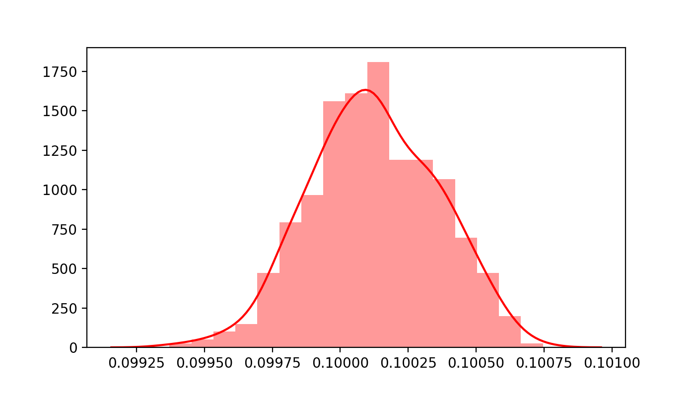
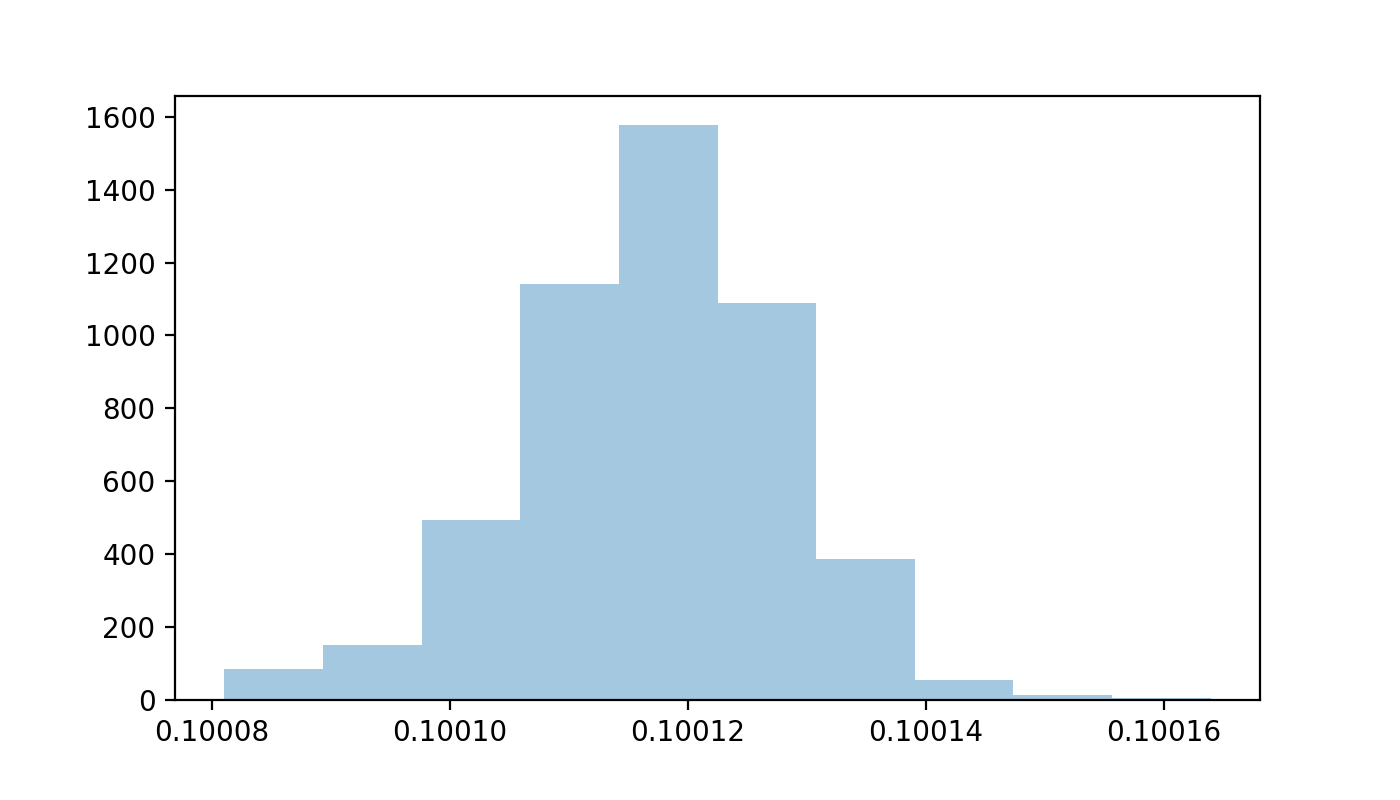
Figure 1: Left: The histogram of samples drew from the posterior distribution of one time dependent coefficient at a single moment. The coefficient is from Burger’s Equation with time varying coefficients. The empirical distribution approximates a Gaussian distribution. The median estimator is $0.100116$. Right: The corresponding sampling distribution for the median estimator obtained by bootstrapping. The original samples are generated by a Gibbs sampler in BGL-SS. The corresponding 95% confidence interval for the estimator is $[0.10009149,0.10013647]$.

4 Numerical results

4.1 Comparison of Algorithms

We test the threshold BGL-SS algorithm on three kinds of dynamic models: Burger’s Equation with time-dependent coefficients, advection-diffusion equation with spatial dependency, and Kuramoto-Sivashinsky equation with spacial dependency. For comparison, two other methods are applied: SGTR [27] and group Lasso [28], on the same dataset. White noise is also added to the dataset to test the performance of each algorithm in a noise rich environment, which is common in real life.

4.1.1 Burger’s Equation

Let us consider a typical example of PDE. In Burger’s equation

$$\frac{\partial u}{\partial t}+\mu u\frac{\partial u}{\partial x}=\nu\frac{\partial^{2}u}{\partial x^{2}}$$ (21)

$\mu$ is set to be a time dependent oscillating coefficient, and $\nu$ to be constant throughout time. Using SciPy function odeint, the equation can be numerically solved. We use the tool functions from [27] and follow their way of calculating derivatives and handling the equation. Twenty candidate terms in the partial differential equation, with powers of $u$ up to third order multiplying derivatives of $u$ with respect to $x$ up to fourth order, are considered.

Set the coefficients and the initial condition:

$$\begin{array}[]{c}\mu=1+\sin(t)/4,\quad\nu=0.1\\ u(x,0)=\exp[-(x+1)^{2}]\end{array}$$ (22)

and we get the numeral solutions as in Figure 2.

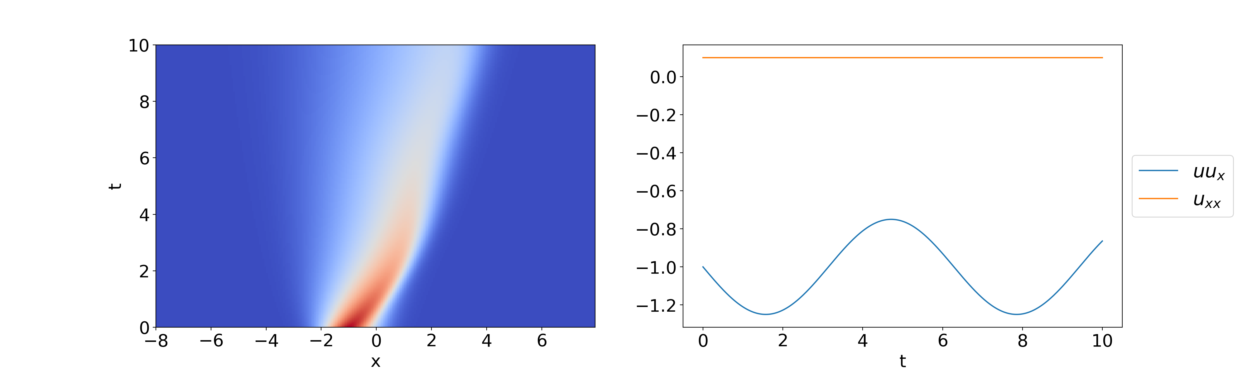
Figure 2: Left: Numeral solution of Burger’s equation, with initial conditions stated in (22). Right: Time varying coefficients in Burger’s equation.

The numeral solutions are then used to generate derivatives and construct the linear system in (7). Threshold BGL-SS is used along with SGTR and Group Lasso to solve the same regression. The results are shown in Figure 3.

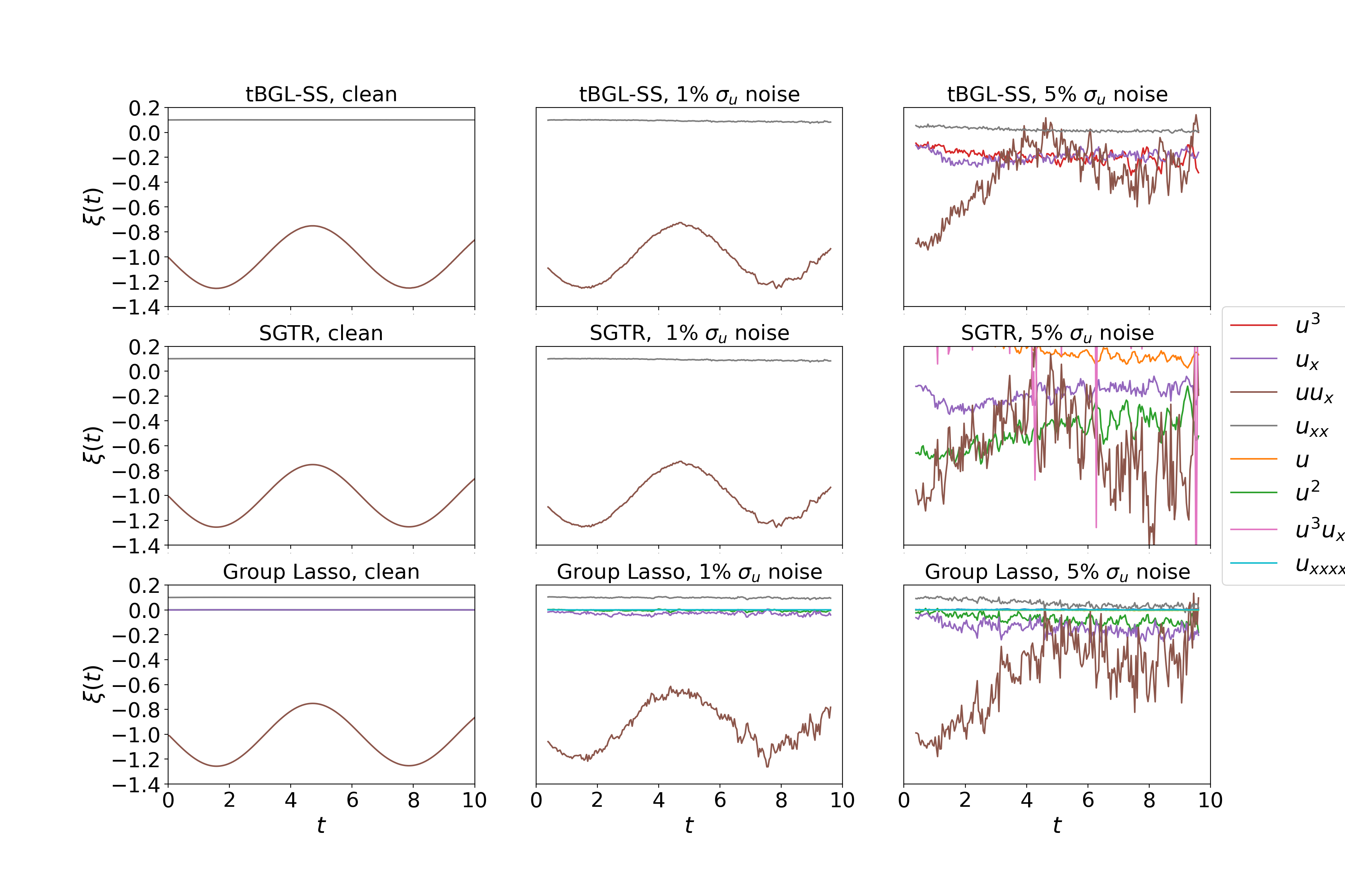
Figure 3: Nine experiments conducted on data with three different levels of noise, Left: Clean, Middle: 1% $\sigma_{u}$ noise, Right: 5% $\sigma_{u}$ noise using three methods, Top: tBGL-SS, Middle: SGTR, and Bottom: Group Lasso in learning Burger’s equation.

Three algorithms are tested with three different levels of white noise added to the data. For threshold BGL-SS, two types of thresholds are applied: a threshold of root mean square ($t_{RMS}$), and a threshold of group error bar ($t_{GE}$) as in (18). Upon the clean data and the 1% $\sigma_{u}$ noise data, a $t_{RMS}=0.02$ is used. When the noise is risen to 5%, $t_{RMS}$ changes to $0.01$. The $t_{GE}=0.1$ in all three experiments. The $\lambda$ of the Lasso is calculated using Monte Carlo EM algorithm [31, 33]. For SGTR and group Lasso, several solutions with different settings of parameters are generated, and the model with the lowest AIC-like loss is chosen.

When the noise level is low or none, both tBGL-SS and SGTR yield good results, while group Lasso failed to exclude some coefficients constantly close to zero, and the output is least fit to the true model. But when the noise is at a relatively high level, all three algorithms fail to identify the terms and coefficient values of the embedded partial differential equation. Nevertheless, threshold BGL-SS and group Lasso appear to be more robust for larger noise than SGTR.

An advantage of tBGL-SS is that the error bars (or bands) can easily be constructed. An example of sample standard deviation error bands is illustrated in Figure 4. Note that the width of the shaded area is exaggerated by 10 times because the original intervals are thinner than the curve line thus cannot be seen. Confidence intervals of median estimators can also be used as an alternative to error bars, and their width would be even thinner.

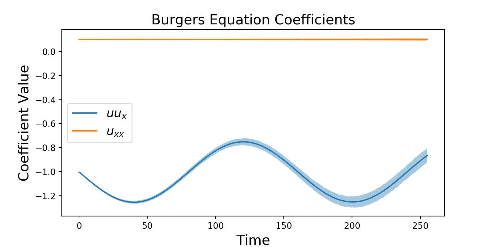
Figure 4: The shaded area represents the standard deviations of coefficients at each moment. Any points in the area is within one SD from the median. The width of the area is magnified by $10$ times.

4.1.2 Advection-Diffusion Equation

Our second example aims to test whether tBGL-SS is able to identify spatially dependent coefficients. The Advection-Diffusion equation is used:

$$\frac{\partial u}{\partial t}=\frac{\partial(\mu u)}{\partial x}+\nu\frac{\partial^{2}u}{\partial x^{2}}=\frac{\partial\mu}{\partial x}u+\mu\frac{\partial u}{\partial x}+\nu\frac{\partial^{2}u}{\partial x^{2}}$$ (23)

Here we let $\mu$ be a spatially varying coefficient. The values of coefficients and the initial condition is set as follows:

$$\begin{array}[]{c}\mu=-1.5+\cos(0.4\pi x),\quad\nu=0.1\\ u(0)=\cos(0.4\pi x)\end{array}$$ (24)

We solve the partial differential equation within the spatial range $[-5,5]$ from $t=0$ to $5$ as shown in Figure 5.

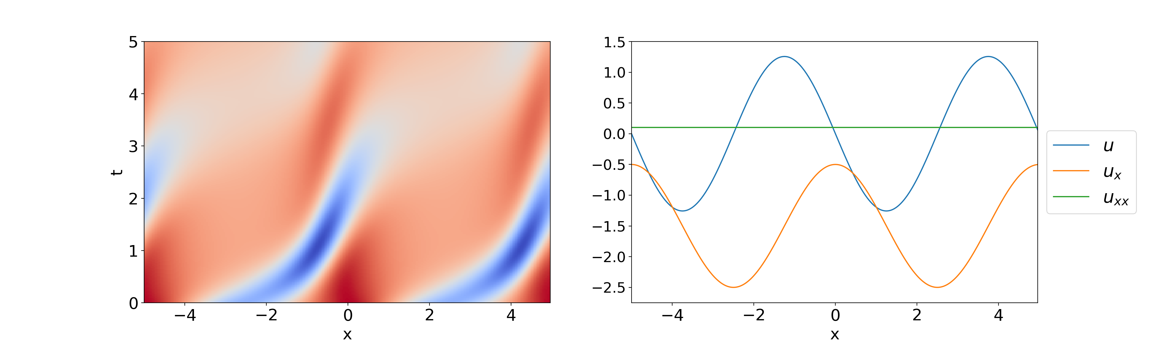
Figure 5: Left: Numeral solution of a spatially dependent Advection-Diffusion Equation, with initial conditions stated in (24). Right: Time varying coefficients in the Advection-Diffusion equation.

We still use threshold BGL-SS, SGTR, and Group Lasso respectively, on three noise levels. The results are presented in Figure 6. For threshold BGL-SS, a $t_{RMS}=0.02$ is applied on the clean data and the 1% $\sigma_{u}$ noise data, and $t_{RMS}=0.01$ for the 2% $\sigma_{u}$ noise data. The $t_{GE}=0.08$ in all three experiments. More iterations in the Gibbs sampler are used in the 2% noise situation. For SGTR and group Lasso, the best parameters, corresponding to the model with the lowest AIC-like loss, is chosen automatically.

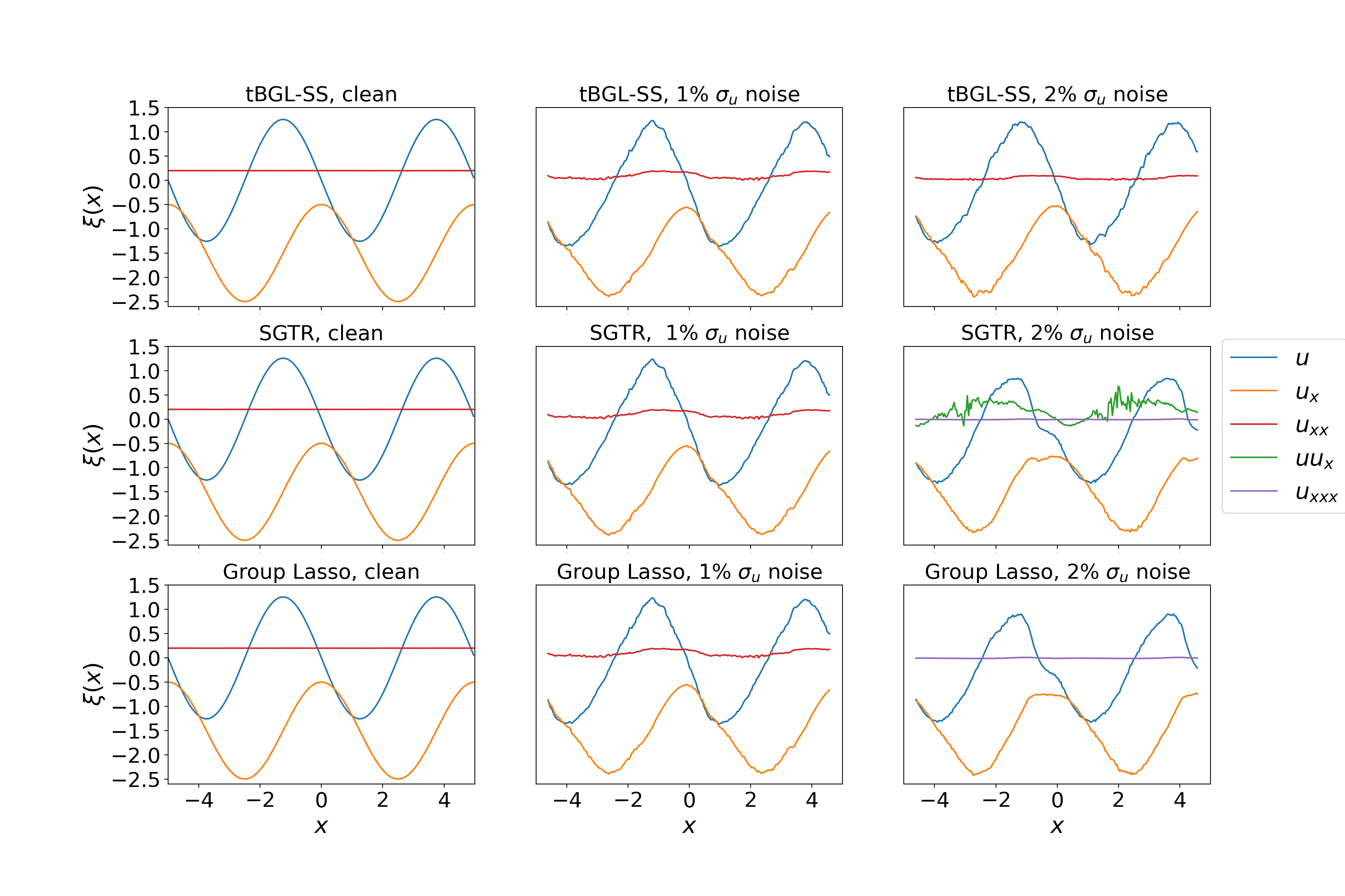
Figure 6: Nine experiments conducted on data with three different levels of noise, Left: Clean, Middle: 1% $\sigma_{u}$ noise, Right: 2% $\sigma_{u}$ noise using three methods, Top: tBGL-SS, Middle: SGTR, Bottom: Group Lasso in learning Advection-Diffusion equation.

The three methods work equally accurately when the data is clean and with small noise. But when larger noise is added, threshold BGL-SS seems to work better than SGTR and Group Lasso. Both Group Lasso and SGTR failed to include the term $u_{xx}$ but instead identified other false terms.

4.1.3 Kuramoto-Sivashinsky Equation

The third test example we use is a Kuramoto-Sivashinsky Equation:

$$\frac{\partial u}{\partial t}=\alpha u\frac{\partial u}{\partial x}+\beta\frac{\partial^{2}u}{\partial x^{2}}+\gamma\frac{\partial^{4}u}{\partial x^{4}}$$ (25)

Here we let

$$\begin{array}[]{c}\alpha=1+0.25\sin(0.1\pi x)\\ \beta=-1+0.25e^{-\frac{(x-2)^{2}}{5}}\\ \gamma=-1-0.25e^{-\frac{(x+2)^{2}}{5}}\\ u(0)=e^{-x^{2}}\end{array}$$ (26)

and get the solution within the spatial range $[-20,20]$ from $t=0$ to $200$ as in Figure 7.

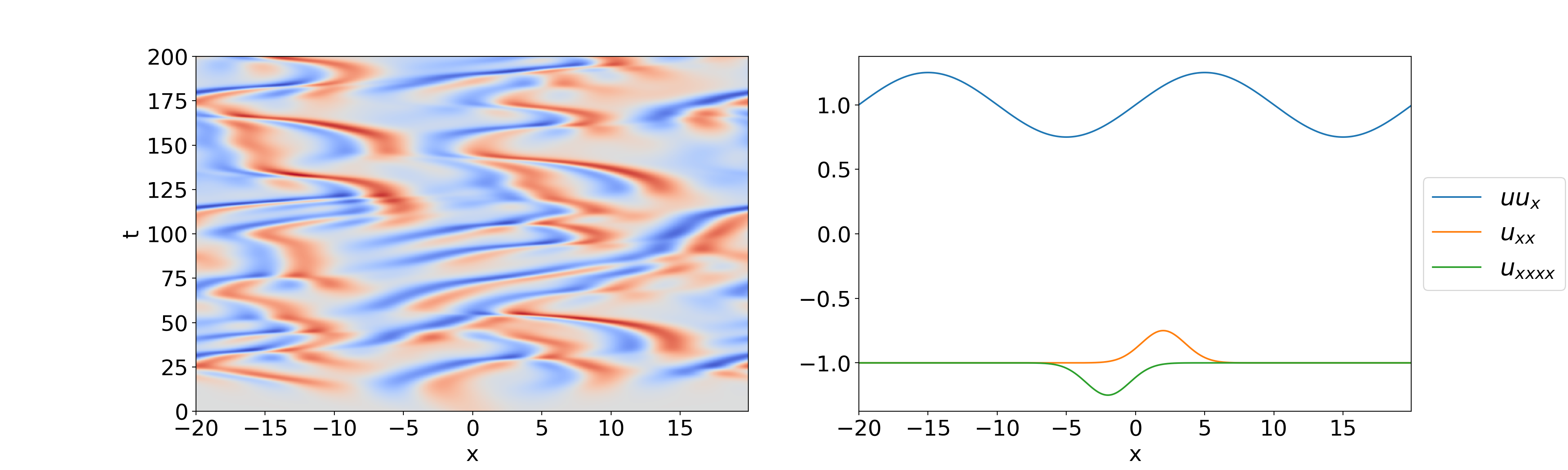
Figure 7: Left: Numeral solution of KS Equation, with initial conditions stated in (26). Right: Time varying coefficients in KS equation.

The KS equation tends to have a chaotic solution, and we use the grid points from $t=100$ to consider the more chaotic part only. When there is 1% noise, none of the three methods can yield a correct result, due to the presence of a fourth order derivative in the equation. Instead, the 0.01% noise is used. For threshold BGL-SS, a $t_{RMS}=0.1$ and a $t_{GE}=0.05$ are applied. The results are shown in Figure 8.

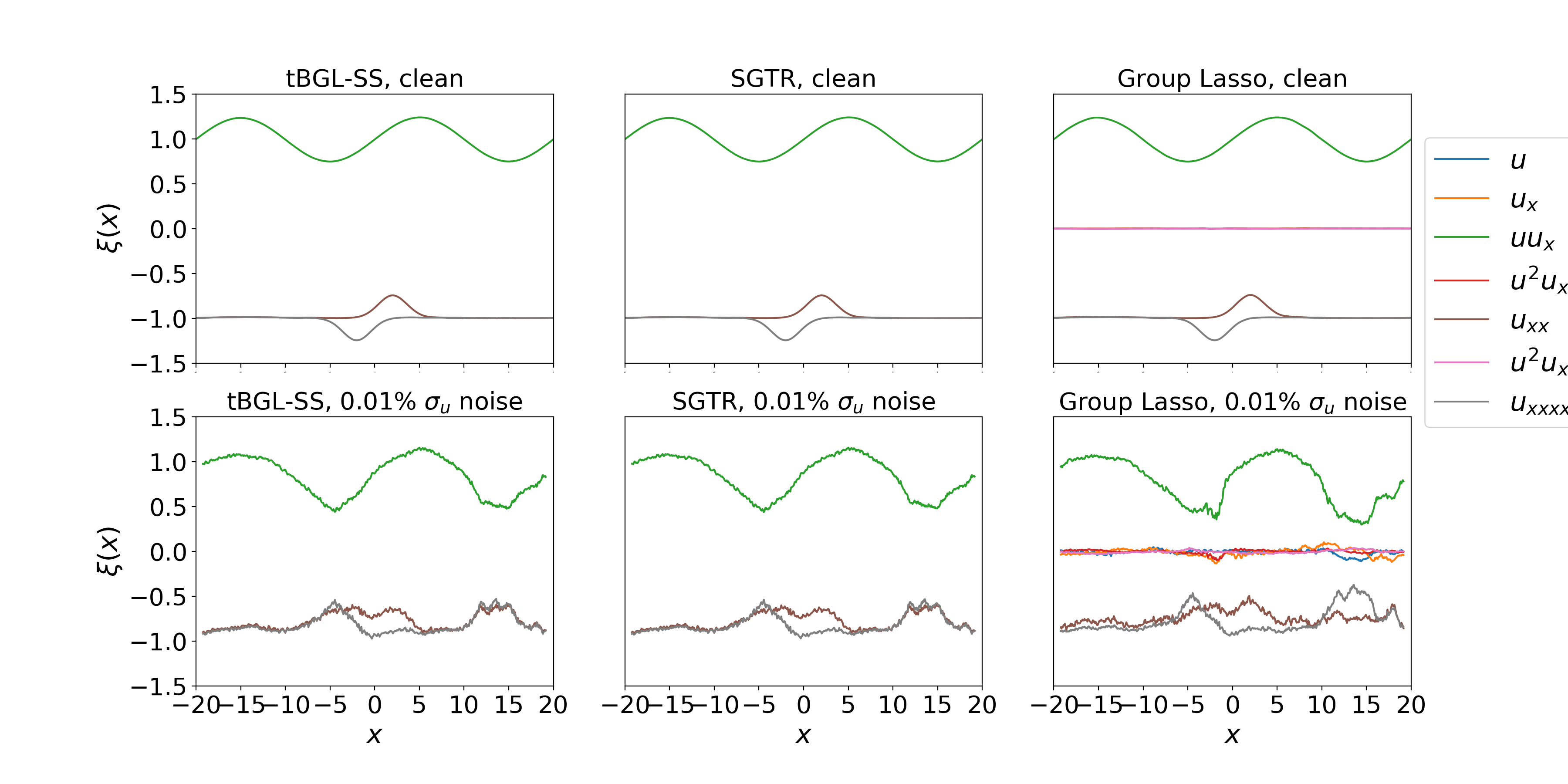
Figure 8: Six experiments conducted on data, Top: with noise, Bottom: without noise, using three methods, Left: tBGL-SS, Middle: SGTR, and Right: Group Lasso in learning KS equation.

4.2 Comparison of Model Selection Criteria

A fundamental task in a thresholding method is to determine the values of the thresholds. In the last subsection, we arbitrarily set some fixed thresholds and got quite good results, but in the real world, this kind of practice may fail easily. A feasible way of choosing the right threshold values is to simply test a series of different thresholds. From a collection of models generated with different settings, the best fitting one is chosen. We have already introduced three different types of criteria. In this subsection, we inspect the three different criteria of model selection: AIC-like loss (19), total error bar (20), and mean square error of coefficients. Note that the mean square error of coefficients cannot be applied if the true values of coefficients are unknown.

Take the identification of advection-diffusion equation (23, 24) for example. If we want to pick a best threshold of group error bar $t_{GE}$ (18), given $t_{RMS}=0.01$, we generate a series of models with different $t_{GE}$ in range $[0.02,0.22]$. Values of the three criteria are calculated respectively for all candidate models. The values are illustrated in Figure 9.

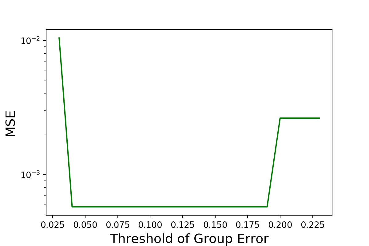
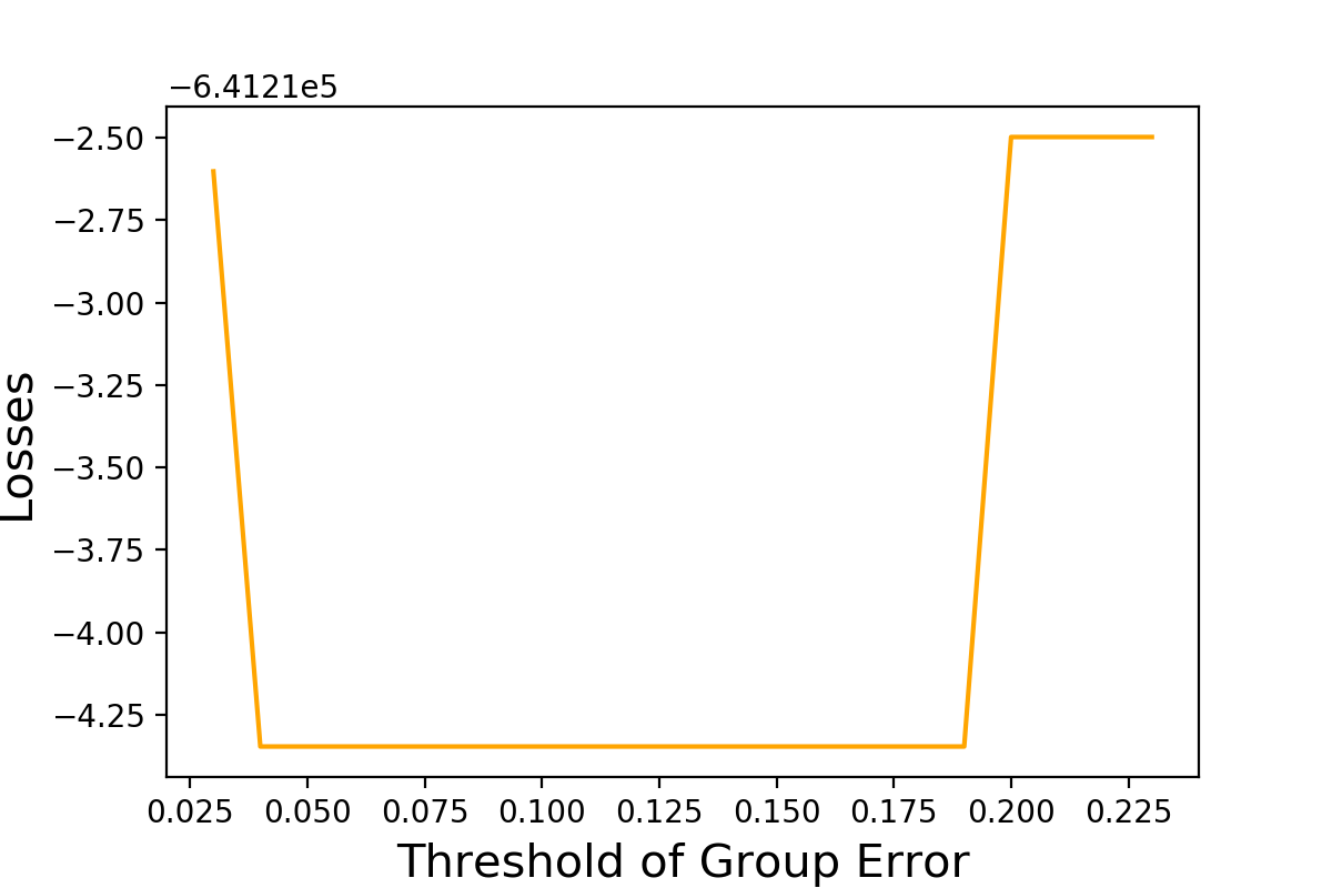
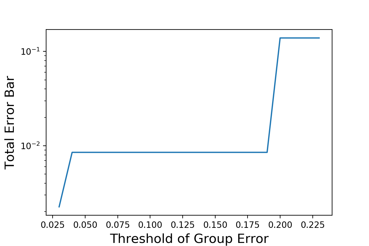
Figure 9: Three criteria of model selection, Left: Mean square error based criterion, Middle: AIC-like loss based criterion, Right: Total error bar based criterion.

It can be inferred that different models will be selected using different criteria. The line of total error bar seems to have an increasing trend. This is natural because the threshold of the group error bar limits nothing other than the widths of error bars. In this case, the loss is a better criterion to avoid redundancy. When we want to select the threshold of root mean square, both loss, and total error bar is feasible.

In practice, if we emphasize the goodness of fit, AIC-like loss should be used. To identify the model with the highest confidence, it is better to use the total error bar criterion instead.

4.3 Dealing with Large Noise

It is hard to identify the correct partial differential equation when the noise is large, as we have shown in the former section. A subsampling method has been proposed in [25], but the time cost is huge with non-constant coefficients. Another way to overcome the problem is to reduce noise in the data preprocessing step. There are various ways to do this, and in our paper, we only consider three of them: moving average, Savitzky-Golay filter [34] and filtfilt in SciPy. We use the example of Burger’s equation in (21, 22), with 5% noise added, to compare the three methods.

The mean square error of the processed data to the original clean data can be used for the evaluation of the filter’s ability:

$$\text{MSE of $u^{\prime}$}=\frac{\sum_{i=1}^{n}\sum_{j=1}^{m}[u^{\prime}(x_{i},t_{j})-u(x_{i},t_{j})]^{2}}{mn}$$ (27)

The data we used with 5% white noise added have a mean square error of $8.099\times 10^{-5}$.

When using the moving average, the window size should be determined first. Draw the MSE of smoothed data against window size, we have the graph in Figure 10. The figure implies the best window width should be 13, where the MSE of processed data reaches its minimum ($7.683\times 10^{-6}$). Feeding the smoothed data to our threshold BGL-SS algorithm, the coefficients can be correctly identified as shown in Figure 11, where the MSE of coefficients is $7.361\times 10^{-5}$. This is much better than that without the usage of moving average ($\text{MSE}=0.04244$). However, the moving average method has a few limitations. First, the edge of the dataset is cut. Second, it performs badly near the extremum as it tends to smooth them as well.

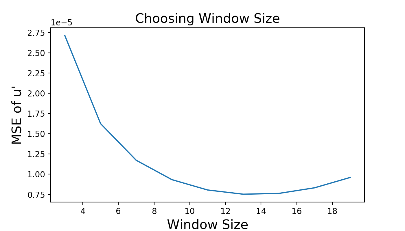
Figure 10: Nine choices of moving average windows and their mean square errors of processed data. When window size is 13, MSE reaches minimum ($7.683\times 10^{-6}$).

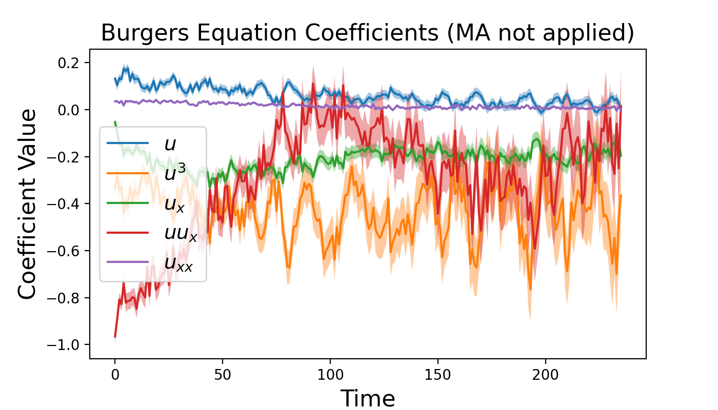
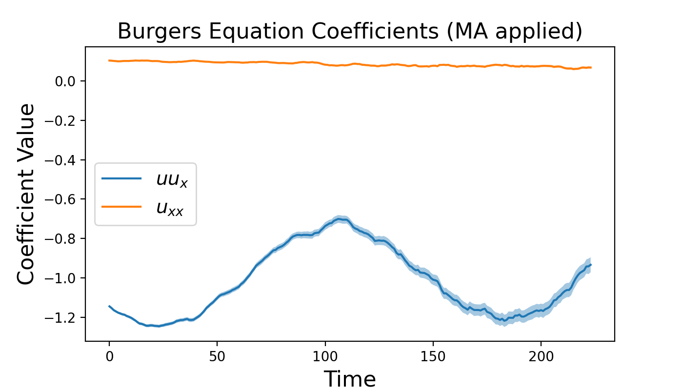
Figure 11: Left: The coefficients identified in the Burger’s equation example, with 5% noise. Error bands for the coefficients are illustrated. Right: The coefficients identified from the same dataset, except for the noise preprocessed using moving average.

Savitzky-Golay filter can track the signal more closely than the moving average. Also, it will not change the shape of data. The filter also needs a window size to run. If the MSE of processed data is plotted against window size the same way, we can easily see that the MSE will reach the minimum ($6.504\times 10^{-6}$) when the window width is 37. Applying tBGL-SS on the smoothed data, the MSE of the coefficient is $7.363\times 10^{-5}$, which is better than that of moving average. Notice that a large window size may distort the identification of coefficients.

The filtfilt filter in SciPy is a forward-backward filter. Instead of window size, the critical frequency in the lowpass Butterworth filter shall be set in advance. We discover that when the critical frequency is 0.0725, MSE reaches its minimum, $7.435\times 10^{-6}$. The MSE of coefficients given by tBGL-SS is $6.945\times 10^{-5}$, which is at the same level as the Savitzky-Golay filter.

5 Conclusions

In this paper, we introduced a robust Bayesian sparse learning algorithm based on Bayesian group Lasso with spike and slab prior [33], to identify the partial differential equations with temporal or spatial varying coefficients. The basic idea of PDE discovery with non-constant coefficients is to select a collection of candidate terms in the PDEs, and treat the variable coefficient of each term as a group of features in the group sparse regression problem [12, 27]. Bayesian group Lasso can ensure group sparsity of the posterior median estimators, using spike and slab priors [33]. We also designed a thresholding mechanism to speed up the Bayesian group Lasso algorithm in big data scenarios, which are common in the PDE discovery tasks.

Extant approaches can hardly quantify the uncertainties of each coefficient, while our method is capable of sampling from the posterior distribution of coefficients using a Gibbs sampler, and provide an estimation of the standard deviation, errors, and confidence intervals. Moreover, uncertainty can be used as a criterion for model selection and threshold setting. We introduced the total error bar and group error bar as the uncertainty criteria for these two purposes. Together with a threshold of root mean square, the group error bar threshold provides us with a new dimension of choosing thresholds, which enables us to identify the correct terms in some specific situations where other non-Bayesian threshold methods cannot.

We used three examples to test whether our method is robust and effective, compared to other group variable selection methods. The performance of our method is as good as or better than SGTR [27] and group Lasso [28] with clean data. When there is noise, our algorithm is as effective as group Lasso, and often works better than SGTR. When the noise is relatively large, all of the three tested algorithms failed to detect the correct form of PDEs. To deal with such a grand challenge, we proposed to employ some preprocessing methods of noise reduction. Numerical results indicate that those preprocessing methods can greatly reduce noise and detect the correct form of PDEs.

This work did not involve any active collection of human data, but only computer simulations.

All data used in this manuscript are publicly available on
http://www.math.purdue.edu/~lin491/data/LETDC

AC conceived the mathematical models, implemented the methods, designed the numerical experiments, interpreted the results, and wrote the paper. GL supported this study and reviewed the final manuscript. All authors gave final approval for publication.

We report no competing interests.

We gratefully acknowledge the support from the National Science Foundation (DMS-1555072, DMS-1736364, CMMI-1634832, and CMMI-1560834), and Brookhaven National Laboratory Subcontract 382247, ARO/MURI grant W911NF-15-1-0562, and U.S. Department of Energy (DOE) Office of Science Advanced Scientific Computing Research program DE-SC0021142.

References

- [1] J. R. Koza, J. R. Koza, Genetic programming: on the programming of computers by means of natural selection, Vol. 1, MIT press, 1992.
- [2] J. Bongard, H. Lipson, Automated reverse engineering of nonlinear dynamical systems, Proceedings of the National Academy of Sciences 104 (24) (2007) 9943–9948.
- [3] M. Schmidt, H. Lipson, Distilling free-form natural laws from experimental data, science 324 (5923) (2009) 81–85.
- [4] M. Raissi, P. Perdikaris, G. E. Karniadakis, Physics informed deep learning (part i): Data-driven solutions of nonlinear partial differential equations, arXiv preprint arXiv:1711.10561.
- [5] M. Raissi, P. Perdikaris, G. E. Karniadakis, Physics informed deep learning (part ii): Data-driven discovery of nonlinear partial differential equations, arXiv preprint arXiv:1711.10566.
- [6] Z. Long, Y. Lu, X. Ma, B. Dong, Pde-net: Learning pdes from data, arXiv preprint arXiv:1710.09668.
- [7] M. Raissi, P. Perdikaris, G. E. Karniadakis, Multistep neural networks for data-driven discovery of nonlinear dynamical systems, arXiv preprint arXiv:1801.01236.
- [8] Z. Long, Y. Lu, B. Dong, Pde-net 2.0: Learning pdes from data with a numeric-symbolic hybrid deep network, Journal of Computational Physics 399 (2019) 108925.
- [9] S. H. Rudy, J. N. Kutz, S. L. Brunton, Deep learning of dynamics and signal-noise decomposition with time-stepping constraints, Journal of Computational Physics 396 (2019) 483–506.
- [10] M. Raissi, P. Perdikaris, G. E. Karniadakis, Machine learning of linear differential equations using gaussian processes, Journal of Computational Physics 348 (2017) 683–693.
- [11] M. Raissi, G. E. Karniadakis, Hidden physics models: Machine learning of nonlinear partial differential equations, Journal of Computational Physics 357 (2018) 125–141.
- [12] S. L. Brunton, J. L. Proctor, J. N. Kutz, Discovering governing equations from data by sparse identification of nonlinear dynamical systems, Proceedings of the National Academy of Sciences 113 (15) (2016) 3932–3937.
- [13] N. M. Mangan, S. L. Brunton, J. L. Proctor, J. N. Kutz, Inferring biological networks by sparse identification of nonlinear dynamics, IEEE Transactions on Molecular, Biological and Multi-Scale Communications 2 (1) (2016) 52–63.
- [14] L. Boninsegna, F. Nüske, C. Clementi, Sparse learning of stochastic dynamic equations, arXiv preprint arXiv:1712.02432.
- [15] G. Tran, R. Ward, Exact recovery of chaotic systems from highly corrupted data, Multiscale Modeling & Simulation 15 (3) (2017) 1108–1129.
- [16] H. Schaeffer, G. Tran, R. Ward, Learning dynamical systems and bifurcation via group sparsity, arXiv preprint arXiv:1709.01558.
- [17] H. Schaeffer, Learning partial differential equations via data discovery and sparse optimization, in: Proc. R. Soc. A, Vol. 473, The Royal Society, 2017, p. 20160446.
- [18] H. Schaeffer, S. G. McCalla, Sparse model selection via integral terms, Physical Review E 96 (2) (2017) 023302.
- [19] H. Schaeffer, G. Tran, R. Ward, Extracting sparse high-dimensional dynamics from limited data, arXiv preprint arXiv:1707.08528.
- [20] N. M. Mangan, J. N. Kutz, S. L. Brunton, J. L. Proctor, Model selection for dynamical systems via sparse regression and information criteria, Proc. R. Soc. A 473 (2204) (2017) 20170009.
- [21] E. Kaiser, J. N. Kutz, S. L. Brunton, Sparse identification of nonlinear dynamics for model predictive control in the low-data limit, arXiv preprint arXiv:1711.05501.
- [22] J.-C. Loiseau, S. L. Brunton, Constrained sparse galerkin regression, Journal of Fluid Mechanics 838 (2018) 42–67.
- [23] S. H. Rudy, S. L. Brunton, J. L. Proctor, J. N. Kutz, Data-driven discovery of partial differential equations, Science Advances 3 (4) (2017) e1602614.
- [24] S. Zhang, G. Lin, Robust data-driven discovery of governing physical laws with error bars, Proceedings of the Royal Society A: Mathematical, Physical and Engineering Sciences 474 (2217) (2018) 20180305.
- [25] S. Zhang, G. Lin, Robust data-driven discovery of governing physical laws using a new subsampling-based sparse bayesian method to tackle four challenges (large noise, outliers, data integration, and extrapolation), arXiv preprint arXiv:1907.07788.
- [26] R. Tibshirani, Regression shrinkage and selection via the lasso, Journal of the Royal Statistical Society. Series B (Methodological) (1996) 267–288.
- [27] S. Rudy, A. Alla, S. L. Brunton, J. N. Kutz, Data-driven identification of parametric partial differential equations, SIAM Journal on Applied Dynamical Systems 18 (2) (2019) 643–660.
- [28] M. Yuan, Y. Lin, Model selection and estimation in regression with grouped variables, Journal of the Royal Statistical Society: Series B (Statistical Methodology) 68 (1) (2006) 49–67.
- [29] J. Friedman, T. Hastie, R. Tibshirani, A note on the group lasso and a sparse group lasso, arXiv preprint arXiv:1001.0736.
- [30] S. Chen, A. Shojaie, D. M. Witten, Network reconstruction from high-dimensional ordinary differential equations, Journal of the American Statistical Association 112 (520) (2017) 1697–1707.
- [31] T. Park, G. Casella, The bayesian lasso, Journal of the American Statistical Association 103 (482) (2008) 681–686.
- [32] M. Kyung, J. Gill, M. Ghosh, G. Casella, et al., Penalized regression, standard errors, and bayesian lassos, Bayesian Analysis 5 (2) (2010) 369–411.
- [33] X. Xu, M. Ghosh, et al., Bayesian variable selection and estimation for group lasso, Bayesian Analysis 10 (4) (2015) 909–936.
- [34] A. Savitzky, M. J. Golay, Smoothing and differentiation of data by simplified least squares procedures., Analytical chemistry 36 (8) (1964) 1627–1639.