Effective screening of medium-assisted Van der Waals interactions between embedded particles

Abstract

The effect of an implicit medium on dispersive interactions of particle pairs is discussed and simple expressions for the correction relative to vacuum are derived. We show that a single point Gauss quadrature leads to the intuitive result that the vacuum van der Waals $C_{6}$ coefficient is screened by the permittivity squared of the environment evaluated near to the resonance frequencies of the interacting particles. This approximation should be particularly relevant if the medium is transparent at these frequencies. In the manuscript, we provide simple models and sets of parameters for commonly used solvents, atoms and small molecules.

1 Introduction

Van der Waals forces are the fundamental interactions between two neutral and polarisable particles [1, 2, 3]. These forces prevail in holding together many materials and play an important role in living organisms, such as geckos walking on smooth surfaces [4]. They have also found increasing importance in technological applications such as microelectromechanical and nanoelectromechanical components [5]. During recent years these forces have been well-studied in several experiments [6, 7, 8, 9] and in theory [10, 11, 12, 13].

Despite their Coulombic origin dispersive forces are among the weakest forces in nature. Time-dependent perturbation theory suggests their interpretation as being caused by ground-state fluctuations of the electromagnetic fields. This view has been taken in Casimir theory [10] dealing with two dielectric plates in vacuum as well as in colloidal systems [14], namely the stabilisation of hydrophobic suspensions of particles in dilute electrolytes [15]. Alternative approaches derive dispersion forces from position-dependent ground-state energies of the coupled field–matter system [1, 10, 16]. These descriptions are restricted to partners interacting in vacuum. Natural systems such as colloids or proteins are often embedded in and environment such as a solvent or a matrix.

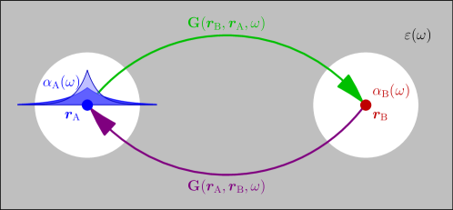
Figure 1: Illustration of two particles (with polarizabilities $\alpha_{\rm A,B}(\omega)$ located at positions $\bm{r}_{\rm A,B}$. The particles are embedded in a medium with permittivity $\varepsilon(\omega)$ (grey area) where a medium excluded area surrounding each particle is formed. Interactions described by the Greens functions $\bf{G}$ are indicated. See text for details.

The impact of an effective medium on dispersive interactions of two particles ${\rm A,B}$ is illustrated in Fig. 1. We adopt the simplification of considering point particles characterised by their frequency-dependent polarizabilities $\alpha_{\rm A,B}(\omega)$ embedded in an effective medium characterised by its frequency-dependent permittivity $\varepsilon(\omega)$. In this picture the Van der Waals potential may be expressed as[13]

$$U({\bm{r}}_{\rm A},{\bm{r}}_{\rm B})=-\frac{\hbar\mu_{0}^{2}}{2\pi}\int\limits_{0}^{\infty}\mathrm{d}\xi\,\xi^{4}\operatorname{Tr}\left[\alpha_{\rm A}({\rm i}\xi)\cdot{\bf{G}}({\bm{r}}_{\rm A},{\bm{r}}_{\rm B},{\rm i}\xi)\cdot\alpha_{\rm B}({\rm i}\xi)\cdot{\bf{G}}({\bm{r}}_{\rm B},{\bm{r}}_{\rm A},{\rm i}\xi)\right]\,,$$ (1)

where the Green functions $\bf{G}$ represent the properties of the field including the medium. One may picturize $\bf{G}$ as describing the interaction between both particles via the exchange of virtual photons. Equation (1) has to be read from right to left: a virtual photon ${\rm i}\xi$ is created at position ${\bm{r}}_{\rm A}$ and propagates to particle B, which is expressed by the Green function ${\bf{G}}({\bm{r}}_{\rm B},{\bm{r}}_{\rm A},{\rm i}\xi)$. At this point it interacts with the polarizability of particle B, $\alpha_{\rm B}({\rm i}\xi)$ and is back-scattered to particle A, again expressed by the Green function ${\bf{G}}({\bm{r}}_{\rm A},{\bm{r}}_{\rm B},{\rm i}\xi)$, where it interacts with particle A. The sum (integral) over all possible virtual photons yields the total Van der Waals interaction.

The presence of a medium as the environment has two distinct effects influencing dispersive interactions between A and B:

• Deformation of the particle’s electron density: Caused by the short distances between the considered particles and the environmental particles, its wave function is modified compared to the one of the free particle [17]. This phenomenon is depicted for particle A in Fig. 1 by the blue (probability of presence) for the free particle and the semitransparent blue area for the confined particle. This deforming effect affects the polarizabilities of both particles $\alpha_{\rm A,B}({\rm i}\xi)$ in the Van der Waals interaction (1).

• Screening of the virtual photon’s propagation: In Figure 1, it can be observed that the virtual photon has to pass the medium. This can be approximated [18] to lead to a damping by $1/\varepsilon({\rm i}\xi)$ for each propagation direction. This process leads to the excess polarizability models [18, 19].

Applying the above to Eq. (1) for a bulk material, the medium-assisted Van der Waals interaction between two particles A and B embedded in a medium with permittivity $\varepsilon(\omega)$ separated by the distance $d$ in the nonretarded limit reads [18, 13, 14]

$$U_{\rm vdW}(d)=-\frac{C_{6}}{d^{6}}\,,\quad C_{6}=\frac{3\hbar}{16\pi^{3}\varepsilon_{0}^{2}}\int\limits_{0}^{\infty}\frac{\alpha_{\rm A}^{\star}({\rm i}\xi)\alpha_{\rm B}^{\star}({\rm i}\xi)}{\varepsilon^{2}({\rm i}\xi)}{\rm d}\xi\,,$$ (2)

with the reduced Planck constant $\hbar$ and the vacuum permittivity $\varepsilon_{0}$. The $\alpha^{\star}_{\rm A,B}({\rm i}\xi)$ are understood to be modified by the presence of the medium.

The procedure to estimate medium-assisted dispersion interactions by the integral (2) is challenging in practical calculations as the polarizabilities as well as the permittivity have to be known over the full frequency range. Furthermore, this integral can get very complex depending on the environmental medium. For instance, the most-commonly applied medium is water, whose currently most exact model consists of 19 damped oscillators, 7 for the infrared and 12 for the ultraviolet regime and 2 Debye terms are involved in order to match the experimental data in the low-frequency regime [20].

Practical electronic structure calculations in the spirit of the model presented in Fig. 1 describe the environment by a polarizable continuum model (PCM) [21, 22] based on the static permittivity sufficient for ground state calculations. The workhorse of electronic structure theory is density functional theory (DFT). The most common functional approximations within DFT are known to severely lack the description of dispersion interactions. This can be corrected by modifying the functional [23] or by adding a dispersive correction to the energy. The latter is in the spirit of our considerations applied by several approaches like the semi-empirical Grimme [24, 25] or the Tkatchenko–Scheffler [26, 27] models. Such models are directly applicable to describe the presence of an explicit environment where all solvent molecules are resolved. Newer developments even take many body interactions into account[27, 25] and should therefore be capable of including nontrivial environmental screening effects at least partly.[28] An explicit description of the environment is computationally very demanding and requires averaging over many different configurations of the environment, e.g. by explicit time propagation.[29]

Form the viewpoint of an implicit approach like the PCM, these corrections are based on free-particle interactions disregarding the presence of the environment. While appropriate in case that both interacting particles are within the same cavity [30] this approach disregards screening by an implicit environment. It was therefore suggested to scale the van der Waals contributions by $\varepsilon^{-2}(\omega)$ with $\omega$ in the optical range [31].

We rationalize this conjecture by presenting an algebraic approximation for the medium-assisted $C_{6}$ coefficient in the following. It is based on a one-point Gauss quadrature rule leading to

$$C_{6}^{\rm app}=\frac{C_{6}^{\rm AB}}{\varepsilon^{2}({\rm i}\overline{\omega})}=\left(\frac{3\varepsilon({\rm i}\overline{\omega})}{1+2\varepsilon({\rm i}\overline{\omega})}\right)^{4}\frac{C_{6}^{\rm vac}}{\varepsilon^{2}({\rm i}\overline{\omega})}\,,$$ (3)

with an averaged main-frequency $\overline{\omega}$ to be determined in what follows. We furthermore show that $\varepsilon^{-2}({\rm i}\overline{\omega})$ might be replaced by $\varepsilon^{-2}(\overline{\omega})$ in the absence of resonances of the environment at the frequency $\overline{\omega}$. The prefactor on the right hand side of Eq. (3) denotes the transition through the interface between the vacuum bubble and the environmental medium according to the Onsager model [32] which is the most-simplest and commonly used excess polarizability model [18]

$$\alpha^{\star}({\rm i}\xi)=\left(\frac{3\varepsilon({\rm i}\xi)}{1+2\varepsilon({\rm i}\xi)}\right)^{2}\alpha({\rm i}\xi)\,.$$ (4)

Due to the resulting linearity between the free-space and the approximated van der Waals coefficient, the impact of excess polarizabilities can be easily included by means of Eq. (3) and will not be considered explicitly in the following.

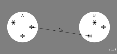
Figure 2: Schematic illustration of the microscopic picture: two ensembles of atoms A and B are embedded in a dielectric medium with permittivity $\varepsilon(\omega)$. The dispersion interaction between the ensembles via the two alternative descriptions as compact objects (mesoscopic picture, see Fig. 1) or via the pairwise interaction as depicted here $E_{ij}$ is screened by the solvent medium.

In this manuscript, we adapt the mesoscopic model to the microscopic models applied, for instance, in DFT simulations. The envisioned medium-assisted situation is depicted in Fig. 2. Two particle ensembles A and B are embedded within a medium with permittivity $\varepsilon(\omega)$ screening the interaction. In models based on electronic structure theory, this interaction is written in the generalised Casimir–Polder form [28]

$$E_{\rm AB}=-\frac{\hbar}{32\pi^{3}\varepsilon_{0}^{2}}\int\limits_{0}^{\infty}\mathrm{d}\xi\int\mathrm{d}{\bm{r}}_{\rm A}\mathrm{d}{\bm{r}}_{\rm A}^{\prime}\mathrm{d}{\bm{r}}_{\rm B}\mathrm{d}{\bm{r}}_{\rm B}^{\prime}\frac{e^{2}}{\varepsilon({\rm i}\xi)\left|{\bm{r}}_{\rm A}-{\bm{r}}_{\rm B}\right|}\frac{e^{2}}{\varepsilon({\rm i}\xi)\left|{\bm{r}}_{\rm A}^{\prime}-{\bm{r}}_{\rm B}^{\prime}\right|}\chi^{\rm A}({\bm{r}}_{\rm A},{\bm{r}}_{\rm A}^{\prime},{\rm i}\xi)\chi^{\rm B}({\bm{r}}_{\rm B},{\bm{r}}_{\rm B}^{\prime},{\rm i}\xi)\,,$$ (5)

which describes the total dispersion energy between the systems A and B, expressed by the electronic density-density responses $\chi^{i}$ for $i={\rm A,B}$. In the presence of a separating medium, these are coupled via the screened Coulomb interaction $e^{2}/\left(4\pi\varepsilon_{0}\varepsilon\left|{\bm{r}}_{\rm A}-{\bm{r}}_{\rm B}\right|\right)$. Applying the dipole approximation to (5), the generalised Casimir–Polder energy gets equivalent to the mesoscopic model obtained via macroscopic quantum electrodynamics Eq. (2)

$$E_{\rm AB} =-\frac{C_{6}^{\rm AB}}{R^{6}}\,,$$ (6)

$$C_{6}^{\rm AB} =\frac{3\hbar}{16\pi^{3}\varepsilon_{0}^{2}}\int\limits_{0}^{\infty}\mathrm{d}\xi\frac{\alpha^{\rm A}({\rm i}\xi)\alpha^{\rm B}({\rm i}\xi)}{\varepsilon^{2}({\rm i}\xi)}\,,$$ (7)

$$\alpha^{i}({\rm i}\xi) =\int\mathrm{d}{\bm{r}}\mathrm{d}{\bm{r}}^{\prime}\,{\bm{r}}{\bm{r}}^{\prime}\chi^{i}({\bm{r}},{\bm{r}}^{\prime},{\rm i}\xi)\,,$$ (8)

where $\alpha^{i}({\rm i}\xi)$ denotes the screened polarizability caused by the deformation of the particle’s electron density $\chi^{i}$ due to the presence of the environment, which does not include the effect described by the excess polarizabilities.

Typically, this interaction is separated into the pairwise interaction of the constituents (the atoms) of systems A and B, as depicted in Fig. 2

$$E_{\rm AB}=\sum_{i,j}E_{i,j}=-\sum_{i,j}f_{ij}(R_{ij})\frac{C_{6}^{ij}}{R_{ij}^{6}}\,,$$ (9)

with $R_{ij}$ denoting the distance between atom $i$ of cloud A and atom $j$ of cloud B, and a correction function $f_{ij}(R_{ij})$ to take short-range phenomena into account. This pairwise separation of the dispersion energy corresponds to the Hamaker approach [33] (or first-order Born series expansion [34]) in macroscopic quantum electrodynamics. Such models are commonly used in modern van-der-Waals–density-functional-theory simulations with tabled vacuum $C_{6}$-coefficients for the different interacting constituents.

Interestingly, within this approach the deformation of the particle’s electron density (I), is expressed via a reduction of the particle’s volume, which, due to the transitivity of the polarizability (8), can directly be expressed by a $C_{6}^{\rm def}$-coefficient for the deformed electron density[26]

$$C_{6}^{\rm def}=\left(\frac{V^{\rm def}}{V^{\rm free}}\right)^{2}C_{6}^{\rm free}\,,$$ (10)

with the reduced particle volume $V^{\rm def}$ and the particle volume and $C_{6}$-coefficient of the free particle, $V^{\rm free}$ and $C_{6}^{\rm free}$, respectively. This assumption is questionable from the macroscopic point of view, as, for instance, the mixing of particle states near interfaces [35] cannot be expressed in such simple way. Further developments[27, 25] take into account similar problems due to non-additivities of the van der Waals interaction [28].

It can be observed that the $C_{6}$-coefficient (7) depends on dispersion of the implicit environmental medium via an integration along the imaginary frequency axis. This fact motivated us to develop a simple model that takes into account the screening of the van der Waals interaction with a similar numerical effort as ordinary DFT simulations in vacuum would require. As the deformation of the particle’s electron density in commonly considered in the form of Eq. (10), the local-field corrections as expressed via excess polarizability models [18] in the form of Eq. (3), we neglect the explicit consideration of these effects within this manuscript.

2 Approximation of medium-assisted C₆-coefficients by Gaussian quadrature

The integral over the imaginary frequency axis for the C₆-coefficient (2) can be carried out by using a single-point Gauss quadrature rule [33, 36]. This method approximates the integral $I$ by

$$I=\int\limits_{0}^{\infty}f(x)g(x)\mathrm{d}x\approx f(x_{0})m_{0}\,.$$ (11)

The values of $x_{0}$ and $m_{0}$ are selected such that the integrals

$$I_{i}=\int\limits_{0}^{\infty}x^{i}g(x)\mathrm{d}x\,,$$ (12)

are exact for $i=0,1$, which guarantees that Eq. (11) is exact for constant or linear functions $f(x)$. This gives $m_{0}=I_{0}$ and $x_{0}=I_{1}/I_{0}$ in agreement with Ref. [36].

Choosing the weight $g(\xi)=\alpha_{\rm A}({\rm i}\xi)\alpha_{\rm B}({\rm i}\xi)$ leads to the relevant mean frequency in Eq. (3)

$$\overline{\omega}=\frac{\int_{0}^{\infty}\,\xi\alpha_{\rm A}({\rm i}\xi)\alpha_{\rm B}({\rm i}\xi)\mathrm{d}\xi}{\int_{0}^{\infty}\,\alpha_{\rm A}({\rm i}\xi)\alpha_{\rm B}({\rm i}\xi)\mathrm{d}\xi}\,.$$ (13)

and Eq. (3) directly. This equation therefore is exact for $\varepsilon^{-2}$ constant or linear in ${\rm i}\xi$. We restrict ourselves to the consideration of non-retarded interactions with respect to the application of the model in density functional theory simulations. A generalisation of the model to include retardation effects is possible and reported in Ref. [36].

3 Comparison between exact and approximated $C_{6}$-coefficients for single oscillator models

The simplest model for the polarizabilities $\alpha_{\rm A,B}$ is that of a single oscillator

$$\alpha_{\rm A,B}({\rm i}\xi)=\frac{A_{\rm A,B}}{1+\left(\xi/\omega_{\rm A,B}\right)^{2}}\,,$$ (14)

with the static value $A_{\rm A,B}$ and the resonance frequency $\omega_{\rm A,B}$. Inserting Eq. (14) into Eq. (13) yields the average main frequency

$$\overline{\omega}=\frac{2}{\pi}\frac{\omega_{\rm A}\omega_{\rm B}}{\omega_{\rm A}-\omega_{\rm B}}\ln\left(\frac{\omega_{\rm A}}{\omega_{\rm B}}\right)$$ (15)

giving $\overline{\omega}=2\omega_{\rm A}/\pi$ for $\omega_{\rm A}=\omega_{\rm B}$.

To illustrate the accuracy of the model assumption (3), we calculated the averaged main frequency (15) for different sets of resonance frequencies $\hbar\omega_{\rm A,B}\in\left[0,10\right]\,\rm{eV}$ for particles dissolved in one of the most-complex media water [20]. We use the parametrization of $\varepsilon({\rm i}\xi)$ for water from Ref. [20] to define the "exact" values of the integral

$$C_{6}^{\rm exact}=\frac{3\hbar A_{\rm A}A_{\rm B}}{16\pi^{3}\varepsilon_{0}^{2}}\int\limits_{0}^{\infty}\frac{\mathrm{d}\xi}{\left[1+(\xi/\omega_{\rm A})^{2}\right]\left[1+(\xi/\omega_{\rm B})^{2}\right]\varepsilon^{2}({\rm i}\xi)}\,,$$ (16)

The comparison between the vacuum and exact Van der Waals coefficients according to Eq. (3) allows to determine the corresponding "exact" averaged main-frequency $\omega_{\rm exact}$

$$\varepsilon({\rm i}\omega_{\rm exact})=\sqrt{\frac{C_{6}^{\rm vac}}{C_{6}^{\rm exact}}}\,.$$ (17)

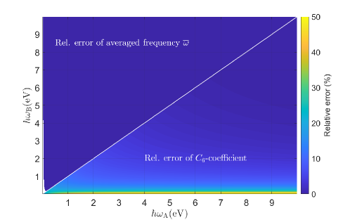
Figure 3: Relative deviations in percent between the approximated averaged frequency $\overline{\omega}$ and the exact main-frequency according to Eq. (3) (top left triangle) and between the approximated and exact van der Waals coefficients (bottom right triangle).

Using these values we can determine the relative deviations of the approximated values according to Eqs. (3) and (15) as

$$\frac{\overline{\omega}-\omega_{\rm exact}}{\omega_{\rm exact}}\,,\quad\frac{C_{6}^{\rm app}-C_{6}^{\rm exact}}{C_{6}^{\rm exact}}\,.$$ (18)

These deviations are generally rather small as depicted in Fig. 3. It can be observed that for materials with a dominant resonance in the microwave, optical, ultraviolet or with higher energies the relative error due to main-frequency approximation is negligible. Only for materials with a dominant resonance in the radio regime and below are not well approximated, which are not very common or realistic materials.

4 Properties of the frequency dependent permittivity

In order to discuss the general properties of the square of the inverse permittivity, we consider its frequency dependence in terms of common approximations. The permittivity may be described in a generalised Debye form

$$\varepsilon_{\rm Debye}(\omega)=1+\sum_{D}\frac{\varepsilon_{D}}{1-{\rm i}\omega\tau_{D}}\,,$$ (19)

or similarly in a generalised Drude form

$$\varepsilon_{\rm Drude}(\omega)=1+\sum_{D}\frac{\varepsilon_{D}\omega_{\rm D}^{2}}{\omega_{\rm D}^{2}-\omega^{2}-{\rm i}\omega\gamma_{D}}\,,$$ (20)

where the two approximations get very similar if we identify $\tau_{D}=3/\omega_{D}$ and $\gamma_{D}=3\omega_{D}$ (see SI). The sums in Eqs. (19) and (20) contain a chosen number of resonators. Generally, the resonator weights $\varepsilon_{D}$ tend to decrease with increasing resonance frequency $\omega_{D}$.

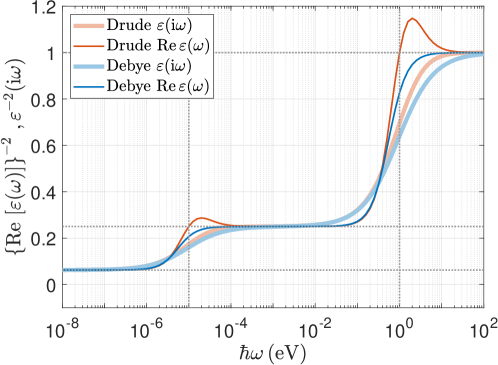
Figure 4: Drude and Debye models with two oscillators with $\hbar\omega_{D}=\left\{10^{-5},1\right\}\,\rm{eV}$ and weights $\varepsilon_{D}=\left\{2,1\right\}$, respectively.

Figure 4 shows $\varepsilon^{-2}({\rm i}\xi)$ in the two approximations for the model case of two resonators only. The $\varepsilon^{-2}({\rm i}\xi)$ is peaked around resonance frequencies, but is rather flat in other regions, where it takes the form of a step-like function. In case that $\overline{\omega}$ does not coincide with a resonance of the environment, $\varepsilon^{-2}({\rm i}\xi)$ can therefore be approximated by a linear function for the main part of the integral (2). The Gaussian quadrature is exact in this case. Figure 4 furthermore shows, that $\varepsilon^{-2}({\rm i}\xi)$ might also be replaced by $1/({\rm Re}[\varepsilon(\omega)])^{2}$ which is well measured and tabulated for many solvents and other environments [37]. Thus, the medium-assisted Van der Waals interaction can effectively be treated via a the screening due to an environmental medium

$$U_{\rm vdW}(d)=-\frac{C_{6}^{\rm vac}}{d^{6}}\frac{1}{\left(\rm{Re}\left[\varepsilon(\overline{\omega})\right]\right)^{2}}\,,$$ (21)

with an averaged main-frequency $\overline{\omega}$ [Eqs. (15) and (31)]. In general the screening coefficient can be evaluated from the dielectric function $\varepsilon(\omega)$ by using the Kramers–Kronig relation [38, 39, 13]

$$\varepsilon({\rm i}\overline{\omega})=1+\frac{2}{\pi}\int\limits_{0}^{\infty}\frac{\omega\,\rm{Im}\,\varepsilon(\omega)}{\omega^{2}+\overline{\omega}^{2}}\mathrm{d}\omega\,.$$ (22)

5 Impact of the model on real molecules

In the following, we apply the model developed to more realistic scenarios and analyse the deviations between the approximation and the exact solutions for the medium-assisted van der Waals interactions. In principle, realistic materials are described via multi oscillator models, which we can distinguish into two classes according to the resonance frequencies: resonances in the ultraviolet regime, which are caused by electronic transitions, and resonances in the infrared regime that are caused by vibrational and rotational modes of the system. To this end, we first consider a two oscillator model with one oscillator within each of these spectral ranges and analyse the model predictions due the ratio between the corresponding oscillator strengths. Afterwards, we consider the interaction between real molecules whose polarizabilities consist of several oscillator models. Finally, we analyse the interaction between atomic compounds in terms of a Hamaker summation according to the common treatment of van der Waals dispersion forces in density functional theory simulations.

5.1 Two-oscillator models

In the previous section and also in Fig. 6, we observe that the resonances of the dielectric response function are dominant in two different spectral ranges — in the infrared and in the ultraviolet range. Hence, we analyse the impact of differently weighted oscillator strengths in our model. We consider a two-oscillator model for the polarizability

$$\alpha({\rm i}\xi)=\frac{C_{\rm IR}}{1+(\xi/\omega_{\rm IR})^{2}}+\frac{C_{\rm UV}}{1+(\xi/\omega_{\rm UV})^{2}}=C_{\rm IR}\left[\frac{1}{1+(\xi/\omega_{\rm IR})^{2}}+\frac{\lambda}{1+(\xi/\omega_{\rm UV})^{2}}\right]\,,$$ (23)

with the ratio between the oscillator strengths

$$\lambda=\frac{C_{\rm UV}}{C_{\rm IR}}\,,$$ (24)

being small ($\lambda\ll 1$) for infrared-dominant species and large ($\lambda\gg 1$) for ultraviolet-dominant species. By inserting Eq. (23) into Eq. (13), this leads to an averaged main-frequency

$$\overline{\omega}= \frac{2}{\pi\left[\left(\omega_{\rm IR}+\lambda\omega_{\rm UV}\right)^{2}+\omega_{\rm IR}\omega_{\rm UV}\left(\lambda+1\right)^{2}\right]}$$

$$\times \Biggl{[}\frac{4\lambda\omega_{\rm IR}\omega_{\rm UV}}{\omega_{\rm IR}-\omega_{\rm UV}}\ln\left(\frac{\omega_{\rm IR}}{\omega_{\rm UV}}\right)+\left(\omega_{\rm IR}+\omega_{\rm UV}\right)\left(\lambda^{2}\omega_{\rm UV}^{2}+\omega_{\rm IR}^{2}\right)\Biggr{]}\,,$$ (25)

satisfying the single-oscillator limits (15). The results for two particles of the some species with the parameters $\hbar\omega_{\rm IR}=0.1\,\rm{eV}$ and $\hbar\omega_{\rm UV}=10\,\rm{eV}$ embedded in water are depicted in Fig. 5. It can be observed the limits of the different dominant regimes are reproduced

$$\overline{\omega}=\frac{2}{\pi}\begin{cases}\omega_{\rm UV}\,,&\text{for}\,\lambda\gg\lambda_{\rm crit}\\ \omega_{\rm IR}\,,&\text{for}\,\lambda\ll\lambda_{\rm crit}\end{cases}\,.$$ (26)

It can be observed that $\lambda_{\rm crit}$ is smaller than unity due to the weighted integral (13). To understand this behaviour quantitatively, we define $\lambda_{\rm crit}$ to be the ratio corresponding to the arithmetical averaged main-frequency $\overline{\omega}(\lambda_{\rm crit})=\left(\omega_{\rm IR}+\omega_{\rm UV}\right)/\pi$. This can be solved analytically and results in

$$\lambda_{\rm crit} =\frac{\sqrt{\rho}}{(1+\rho)(\rho-1)^{2}}\left\{4\rho^{3/2}\ln\rho+2\sqrt{\rho}-2\rho^{5/2}\right.$$

$$\left.+\left[16\rho^{2}\ln\rho\left(\rho\ln\rho+1-\rho^{2}\right)+(\rho-1)^{2}(1+\rho)^{4}\right]^{1/2}\right\}\,,$$ (27)

with the ratio between the resonance frequencies $\rho=\omega_{\rm IR}/\omega_{\rm UV}\ll 1$ being typically much smaller than 1. The resulting $\lambda_{\rm crit}<1$ implies that the averaged main-frequency is typically closer to the ultraviolet resonance unless its resonance is much smaller than that of the infrared resonance.

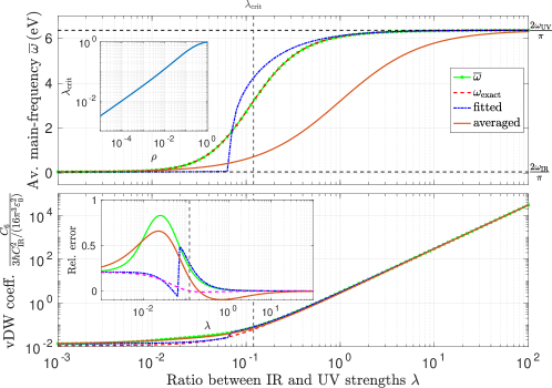
Figure 5: Comparison of the averaged main-frequency $\overline{\omega}$ (top figure) obtained via (25) (green lines), the exact result by solving Eq. (17) (red lines), the fitted to a one-oscillator model (14) (blue lines) and an arithmetically averaged model $\overline{\omega}=2/\pi(\omega_{\rm IR}+\lambda\omega_{\rm UV})/(1+\lambda)$ (orange lines) for a two-oscillator polarizability (23) with the parameters $\hbar\omega_{\rm IR}=0.1\,\rm{eV}$ and $\hbar\omega_{\rm UV}=10\,\rm{eV}$ depending on the ratio between the ultraviolet and infrared oscillator strengths $\lambda$. The asymptotes of the single oscillator limits are the horizontal dashed lines. The critical ratio $\lambda_{\rm crit}$ is drawn by the vertical dashed grey line. The inset of the upper figure illustrates the dependence of the critical ratio on the ratio between the resonance frequencies $\rho=\omega_{\rm IR}/\omega_{\rm UV}$. The bottom figure illustrate the resulting normalised van der Waals coefficients with an inset of corresponding relative errors according to Eq. (18), where furthermore the relative error of the single oscillator treatment is depicted via the magenta line.

Figure 5 illustrates the relevant dependencies of the two-oscillator model. In addition, to the derived two-oscillator model (25), we added a simple weighted averaged main-frequency model

$$\overline{\omega}=\frac{2}{\pi}\frac{\omega_{\rm IR}+\lambda\omega_{\rm UV}}{1+\lambda}\,,$$ (28)

a fit of the two-oscillator model onto a single oscillator model, which can be performed analytically by solving the corresponding least-square equation and by splitting the van der Waals coefficient into its three single oscillator contributions

$$\frac{C_{6}}{3\hbar C_{\rm IR}^{2}/(16\pi^{3}\varepsilon_{0}^{2})}=\int\limits_{0}^{\infty}\frac{\mathrm{d}\xi}{\varepsilon^{2}({\rm i}\xi)\left[1+\left(\xi/\omega_{\rm IR}\right)^{2}\right]^{2}}$$

$$+2\lambda\int\limits_{0}^{\infty}\frac{\mathrm{d}\xi}{\varepsilon^{2}({\rm i}\xi)\left[1+\left(\xi/\omega_{\rm IR}\right)^{2}\right]\cdot\left[1+\left(\xi/\omega_{\rm UV}\right)^{2}\right]}+\lambda^{2}\int\limits_{0}^{\infty}\frac{\mathrm{d}\xi}{\varepsilon^{2}({\rm i}\xi)\left[1+\left(\xi/\omega_{\rm UV}\right)^{2}\right]^{2}}\,.$$ (29)

It can be observed, that the model (25) agrees very well with the exact averaged main-frequency. The corresponding asymptotes are governed by the conditions (26) together with Eq. (27) for $\lambda_{\rm crit}$. Remarkably, the alternative models (weighted average and fit-to-single-oscillator model) strongly deviate for the predictions of the averaged main-frequency, but matches better the van der Waals coefficients of infrared-dominant materials. For ultraviolet-dominant responding species, the presented model predicts better the $C_{6}$-coefficients than the other models. The optimum over the whole range is given by the treatment of each single oscillator (29).

5.2 Multi-oscillator models

The oscillator model (14) can easily be extended to several oscillators

$$\alpha_{\rm A,B}({\rm i}\xi)=\sum_{i}\frac{A_{\rm A,B}^{(i)}}{1+\left(\xi/\omega_{\rm A,B}^{(i)}\right)^{2}}\,,$$ (30)

leading to an averaged main-frequency

$$\overline{\omega}=\frac{2}{\pi}\left(\sum_{i,j}A_{\rm A}^{(i)}A_{\rm B}^{(j)}\frac{\left[\omega_{\rm A}^{(i)}\omega_{\rm B}^{(j)}\right]^{2}}{\left[\omega_{\rm A}^{(i)}\right]^{2}-\left[\omega_{\rm B}^{(j)}\right]^{2}}\ln\left(\frac{\omega_{\rm A}^{(i)}}{\omega_{\rm B}^{(j)}}\right)\right)\left(\sum_{i,j}\frac{A_{\rm A}^{(i)}A_{\rm B}^{(j)}\omega_{\rm A}^{(i)}\omega_{\rm B}^{(j)}}{\omega_{\rm A}^{(i)}+\omega_{\rm B}^{(j)}}\right)^{-1}\,.$$ (31)

As a note of caution, we remark that, as evident from the discussion in Sec. 2, our method may lead to less accurate results for molecules whose relevant transitions span several plateau regions of $\varepsilon({\rm i}\xi)$. In this case, a separate treatment of each oscillator is recommended, as shown in the previous section.

	CH4	NO2	CO2	CO	N2O	O3	O2	N2	H2S	NO
CH4	11.4	12.6	12.6	12.2	12.3	12.7	13.2	12.8	10.3	12.8
NO2	12.6	14.2	14.3	13.7	13.9	14.4	15.0	14.4	11.3	14.5
CO2	12.6	14.3	14.3	13.7	14.0	14.4	15.0	14.4	11.4	14.5
CO	12.2	13.7	13.7	13.1	13.4	13.8	14.4	13.8	11.0	13.9
N2O	12.3	13.9	13.9	13.4	13.6	14.0	14.7	14.0	11.1	14.1
O3	12.7	14.4	14.4	13.8	14.0	14.5	15.2	14.4	11.4	14.6
O2	13.2	15.0	15.0	14.4	14.7	15.2	15.9	15.1	11.9	15.2
N2	12.8	14.4	14.4	13.8	14.0	14.5	15.1	14.4	11.5	14.6
H2S	10.3	11.3	11.4	11.0	11.1	11.4	11.9	11.5	9.3	11.5
NO	12.8	14.5	14.5	13.9	14.1	14.6	15.2	14.6	11.5	14.7

Table 1: Average main-frequencies $\overline{\omega}\,(\rm{eV})$ for different molecule pairs. The corresponding parameters for the polarizabilities are taken from Refs. [18, 40].

In Table 1, averaged main-frequencies are given for different pairs of small molecules. The corresponding polarizabilities are taken from Refs. [18, 40]. It can be observed that the averaged main-frequency is mainly located in the energy range between 10 and 15 eV.

Due to this reduction of the relevant energy range, the dielectric functions of the solvent can be approximated by a single UV oscillator model

$$\varepsilon_{\rm app}({\rm i}\xi)=\frac{\varepsilon_{s}-\varepsilon_{\infty}}{1+\left(\xi/\omega_{\rm UV}\right)^{2}}+\varepsilon_{\infty}\,,$$ (32)

where $\varepsilon_{s}$ is the low frequency permittivity and $\varepsilon_{\infty}$ is the permittivity for large frequencies that may contain contributions of other oscillators at higher frequencies. The dielectric functions of typical solvents are illustrated in Fig. 6. The parametrization of the alcohols are taken from Ref. [41] and that of water from Ref. [20]. These models have been fitted to the reduced response model (32) whose resulting parameters are given in table 2. This reduced model is in good agreement with the original data which can be observed in the inset of Fig. 6. Equation (32) describes a Drude oscillator without damping, which is sufficient for the description of dispersion interactions.

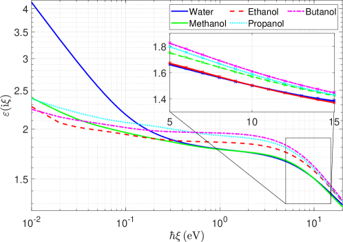
Figure 6: Dielectric function of water and some common solvent alcohols (ethanol, methanol, butanol and propanol) on the imaginary axis.The crosses in the inset illustrate the approximated dielectric functions due to Eq. (32) with the parameters in table 2.

Solvent	$\varepsilon_{\infty}$	$\varepsilon_{s}$	$\omega_{\rm UV}$
Water	1.193	1.766	10.73
Ethanol	1.141	1.853	12.29
Methanol	1.098	1.766	12.46
Butanol	1.154	1.954	11.47
Propanol	1.144	1.921	11.52
Cyclopentane	1.092	1.938	11.65
Cyclohexane	1.096	1.991	11.68
Benzene	1.169	2.199	10.07
Fluorobenzene	1.145	2.088	10.31
Chlorobenzene	1.157	2.264	10.38
Bromobenzene	1.173	2.371	10.33
Pentane	1.080	1.808	13.16
Heptane	1.086	1.857	13.07
Glycerol	1.152	2.152	12.10
Tetrachloromethane	1.103	2.076	12.13

Table 2: Parameters for some solvents according to the reduced single oscillator model (32).

Mol. A	Medium	Mol. B	$C_{6}^{\rm vac}$	$\overline{\omega}$	$\varepsilon({\rm i}\overline{\omega})$	$\varepsilon_{\rm app}({\rm i}\overline{\omega})$	$C_{6}^{\rm app}$	$C_{6}^{\rm exact}$	rel. Dev.
CH4	Water	CH4	116.68	11.35	1.47	1.46	54.48	51.90	4.99%
CO2	Water	N2O	174.42	13.92	1.40	1.41	88.16	81.69	7.91%
NO	Water	H2S	117.12	11.53	1.46	1.46	55.02	52.01	5.80%
CH4	Ethanol	CH4	116.68	11.35	1.53	1.53	50.16	48.76	2.87%
O2	Methanol	H2S	109.06	11.92	1.45	1.45	52.12	49.35	5.61%
N2	Butanol	H2S	120.86	11.52	1.55	1.55	50.15	48.08	4.32%
O2	Propanol	CH4	81.51	13.24	1.48	1.48	37.28	34.74	7.32%

Table 3: Comparison of different molecule combinations (Molecule A and B) with the vacuum Van der Waals coefficient $C_{6}^{\rm vac}\,(10^{79}\rm{Jm}^{6})$, the corresponding averaged main-frequency $\overline{\omega}\,(\rm{eV})$, the exact and approximated (32) dielectric functions evaluated at the averaged main-frequency, the approximated Van der Waals coefficient according to Eq. (3) $C_{6}^{\rm app}\,(10^{79}\rm{Jm}^{6})$, the exact Van der Waals coefficient according to Eq. (2) $C_{6}^{\rm exact}\,(10^{79}\rm{Jm}^{6})$ and the relative deviation of the approximated and exact $C_{6}$-coefficients.

The impact of the model (3) for a selection of interacting particles are given in table 3. The complete list can be found in the supplementary information. It can be seen that the model well-approximates the Van der Waals interactions between both particles within a deviation of roughly 5-10%. We can expect even better agreement for molecules with dominant excitations in the optical or low UV range as these frequencies are further apart from the resonances of the solvent.

5.3 Combination model according to the summation over pairwise atomic interactions

In common density functional theory simulations, the van der Waals interaction between complex molecules is decomposed via the Hamaker approach (pairwise summation) over the atomic constituents of each molecule [26]

$$C_{6}^{\rm AB}=\sum_{a\in\mathcal{A}}\sum_{b\in\mathcal{B}}C_{6}^{ab}\,,$$ (33)

where $\mathcal{A}$ and $\mathcal{B}$ denotes the set of atoms of molecule A and B, respectively, with an effective van der Waals interaction between atom $a$ and $b$ expressed by $C_{6}^{ab}$. Figure 2 illustrates this decomposition. The effective van der Waals interaction between each pair is treated analogously to the screening of the electronic density (10) to be linear in the free-space van der Waals coefficient

$$C_{6}^{ab}\propto C_{6}^{{\rm free},ab}\,.$$ (34)

This ansatz allows us to apply the effective screening to the atomic decomposition of the molecules. Commonly, atomic dynamic polarizabilities are treated by a single Lorentz oscillator with an oscillator strength and a resonant frequency (14) that are given by the static polarizability $\alpha_{\rm A}(0)$ and the van der Waals coefficient for the equal particle pairwise interaction in vacuum

$$C_{6}^{\rm AA}=\frac{3\hbar}{16\pi^{3}\varepsilon_{0}^{2}}\int\limits_{0}^{\infty}\mathrm{d}\xi\left[\frac{\alpha_{\rm A}(0)}{1+\left(\xi/\omega_{0}^{\rm A}\right)^{2}}\right]^{2}=\frac{3\hbar\alpha_{\rm A}^{2}(0)\omega_{0}^{\rm A}}{64\pi^{2}\varepsilon_{0}^{2}}\,.$$ (35)

Thus, the resonance frequency is given by

$$\omega_{0}^{\rm A}=\frac{64\pi^{2}\varepsilon_{0}^{2}C_{6}^{\rm AA}}{3\hbar\alpha_{\rm A}^{2}(0)}\,.$$ (36)

By inserting this (36) into Eq. (15), one finds the averaged main-frequency

$$\overline{\omega}=\frac{128\pi\varepsilon_{0}^{2}}{3\hbar}\frac{C_{6}^{\rm AA}C_{6}^{\rm BB}}{C_{6}^{\rm AA}\alpha_{\rm B}^{2}(0)-C_{6}^{\rm BB}\alpha_{\rm A}^{2}(0)}\ln\left(\frac{C_{6}^{\rm AA}\alpha_{\rm B}^{2}(0)}{C_{6}^{\rm BB}\alpha_{\rm A}^{2}(0)}\right)\,,$$ (37)

which simplifies to

$$\overline{\omega}=\frac{128\pi\varepsilon_{0}^{2}C_{6}^{\rm AA}}{3\hbar\alpha_{\rm A}^{2}(0)}\,,$$ (38)

for two particles of the same species. Table 4 illustrates the averaged main-frequency for different atomic combinations involved in organic particles: carbon, hydrogen, oxygen, nitrogen, sulfur, fluorine, chlorine, bromine and iodine. The parameters for the polarizabilities are taken from Ref. [42]. It can be seen that the resulting parameters are again in the ultraviolet range between 7.25 eV and 15 eV. Thus, the dielectric functions for the different solvents provided in table 2 can be used to determine the screening factors.

$\hbar\overline{\omega}\,(\rm{eV})$	C	H	O	N	S	F	Cl	Br	I
C	7.47	7.44	9.51	8.70	7.76	10.45	8.50	8.34	7.37
H	7.44	7.41	9.47	8.66	7.73	10.40	8.46	8.31	7.34
O	9.51	9.47	12.36	11.21	9.90	13.69	10.93	10.72	9.36
N	8.70	8.66	11.21	10.21	9.05	12.38	9.96	9.77	8.57
S	7.76	7.73	9.90	9.05	8.06	10.89	8.83	8.67	7.64
F	10.45	10.40	13.69	12.38	10.89	15.23	12.06	11.82	10.28
Cl	8.50	8.46	10.93	9.96	8.83	12.06	9.71	9.53	8.37
Br	8.34	8.31	10.72	9.77	8.67	11.82	9.53	9.35	8.22
I	7.37	7.34	9.36	8.57	7.64	10.28	8.37	8.22	7.26

Table 4: The averaged main-frequency for atomic combination of organic particles.

The application of this atomic model has to be taken with a grain of salt because polarizabilities are typically non-additive with respect to the constituents of the considered particle [28]. There are several effects which are not covered by Eq. (33). One of these effects is the rescaling of the free-space van der Waals coefficient due to the particle’s volume (10). Several investigations, in theory [35, 43, 44] and experiment [45, 46], have shown that the largest effect of a surface (respectively a cavity) results in a spectral shift of the particle’s resonance $\Delta\omega$. Such effect can, for instance, be included within this model by applying a Taylor series expansion to Eq. (15) leading to a shift of the averaged main-frequency

$$\Delta\overline{\omega} =\frac{2}{\pi}\left[\frac{\omega_{\rm A}^{2}\Delta\omega_{\rm B}-\omega_{\rm B}^{2}\Delta\omega_{\rm A}}{\left(\omega_{\rm A}-\omega_{\rm B}\right)^{2}}\ln\left(\frac{\omega_{\rm A}}{\omega_{\rm B}}\right)+\frac{\omega_{\rm B}\Delta\omega_{\rm A}-\omega_{rmA}\Delta\omega_{\rm B}}{\omega_{\rm A}-\omega_{\rm B}}\right.$$

$$\left.+\frac{\omega_{\rm A}^{2}-\omega_{\rm B}^{2}-2\omega_{\rm A}\omega_{\rm B}\ln\left(\omega_{\rm A}/\omega_{\rm B}\right)}{\left(\omega_{\rm A}-\omega_{\rm B}\right)^{3}}\Delta\omega_{\rm A}\Delta\omega_{\rm B}\right]\,,$$ (39)

which has to be considered for the evaluation of the screening factor $\varepsilon^{-2}({\rm i}\overline{\omega}+{\rm i}\Delta\overline{\omega})$. Another effect this model can be adapted to is the many-particle interaction behind the pairwise assumption, e.g. the three-body interaction (the Axilrod–Teller potential) that describes the interaction between three polarisable particles. Its strength is given by [47, 48]

$$C_{9}\propto\int\limits_{0}^{\infty}\frac{\alpha_{\rm A}({\rm i}\xi)\alpha_{\rm B}({\rm i}\xi)\alpha_{\rm C}({\rm i}\xi)}{\varepsilon^{n}({\rm i}\xi)}\,,$$ (40)

where $n$ denotes the number of interactions crossing the intermediate medium, e.g. if all three particles belong to three different molecules, than $n=3$, whereas if all constituents belongs to the same molecule than $n=0$. In analogy to Eq. (13) an averaged main-frequency can be derived, which reads for three single-oscillator models

$$\overline{\omega} =\frac{2}{\pi}\frac{\omega_{\rm A}\omega_{\rm B}\omega_{\rm C}}{\omega_{\rm A}+\omega_{\rm B}+\omega_{\rm C}}\frac{1}{\left(\omega_{\rm B}-\omega_{\rm C}\right)\left(\omega_{\rm A}-\omega_{\rm C}\right)\left(\omega)_{\rm A}-\omega_{\rm B}\right)}$$

$$\times\left[\omega_{\rm A}^{2}\ln\left(\frac{\omega_{\rm B}}{\omega_{\rm C}}\right)+\omega_{\rm B}^{2}\ln\left(\frac{\omega_{\rm C}}{\omega_{\rm A}}\right)+\omega_{\rm C}^{2}\ln\left(\frac{\omega_{\rm A}}{\omega_{\rm C}}\right)\right]\,.$$ (41)

Beyond this extension, the model can be adapted to the consideration of higher-order multipoles, e.g. the non-retarded dipole-quadrupole interaction [49]

$$U(r)=-\frac{C_{8}}{r^{8}}\,,$$ (42)

with

$$C_{8}=\frac{90\hbar c}{160\pi^{3}\varepsilon_{0}^{2}}\int\limits_{0}^{\infty}{\rm d}\xi\alpha({\rm i}\xi)\beta({\rm i}\xi)\,,$$ (43)

with the scalar dipole and quadrupole polarizabilities, $\alpha({\rm i}\xi)$ and $\beta({\rm i}\xi)$, respectively. By, for instance, assuming single Lorentz oscillator models (14) to model each response function, the resulting screening effect can be effectively be treated in analogy to Eqs. (15) and (3).

Beyond these extensions, there are some limitations that the model cannot cover: (i) the intermediate regime, where retardation effects start to play a role are not adaptable, because the potential does not factorises into a part depending on the polarizabilities and another part only depending on the dielectric function of the medium [50]; and (ii) in situations, where the interacting atomic systems A and B are so close together that the electronic densities start to overlap and a molecule is formed, the derived model fails due to the coupling dipole-electric field interaction Hamiltonian applied in the whole theory.

6 Conclusion

We have shown that the medium-assisted Van der Waals interaction can effectively be treated as a the screening due to an environmental medium. Single point Gauss quadrature suggests the screening to be the inverse of $\varepsilon({\rm i}\overline{\omega})^{2}$ with an averaged main-frequency $\overline{\omega}$ that depends on the resonances of the interacting molecules. The approximation should be particularly accurate if these resonances are far from the resonances of the medium. Then $\varepsilon({\rm i}\overline{\omega})^{-2}$ might even be replaced by the permittivity evaluated at real frequencies $\varepsilon(\overline{\omega})^{-2}$. Application of the approximation proposed for small molecules with resonances near to these of the solvents reveal still an accuracy of 90-95%.

As embedded molecules in solvents often show their dominating resonances in the optical region, screening of van der Waals interactions by the solvent is greatly suppressed as compared to electrostatic Coulomb interactions. In the extreme, but important case of water, the latter are screened by the factor 1/78 [22] due to its large static polarizability. The permittivity in the optical region is much lower [31], leading to a screening of the van der Waals interaction by $\approx 0.5$ compared to the vacuum case.

Nevertheless, the simple form of our result is useful for adjusting Van der Waals corrections of molecules within implicit solvents [31]. Furthermore, the screening might affect also molecular dynamics calculations in aqueous environment such as the important problem of protein folding [51], or may resolve some of the discrepancies between simulated and experimental dielectric constants [52]. The solvents’ permittivity in the optical range is caused by resonances of the solvents’ electronic system. As classical force fields do not include electrons, the corresponding screening term is missing and therefore also the screening term described here. Modification of the bare Coulomb interaction by the relative permittivity has been shown to improve the description of ion-ion interactions considerably.[53]

Appendix A Drude and Debye formulas for a single resonator

There are different possible forms of approximations for the frequency dependent permittivity. One of the most compact is the Debye relaxation formula for a single resonator which is completely determined by the relaxation time $\tau_{D}$

$$\varepsilon(\omega)=\frac{\varepsilon_{s}-\varepsilon_{\infty}}{1-{\rm i}\omega\tau_{D}}+\varepsilon_{\infty}$$ (44)

with the static permittivity $\varepsilon_{s}$ and the permittivity for infinite frequency $\varepsilon_{\infty}$. This approximation reads at complex frequencies

$$\varepsilon({\rm i}\xi)=\frac{\varepsilon_{s}-\varepsilon_{\infty}}{1+\xi\tau_{D}}+\varepsilon_{\infty}\;.$$ (45)

The Drude form for a single resonance at resonance frequency $\omega_{D}$ and width $\gamma_{D}$ is

$$\varepsilon(\omega)=\frac{(\varepsilon_{s}-\varepsilon_{\infty})\omega_{D}^{2}}{\omega_{D}^{2}-\omega^{2}-{\rm i}\omega\gamma_{D}}+\varepsilon_{\infty}$$ (46)

and for complex frequencies

$$\varepsilon({\rm i}\xi)=\frac{(\varepsilon_{s}-\varepsilon_{\infty})\omega_{D}^{2}}{\omega_{D}^{2}+\xi^{2}+\xi\gamma_{D}}+\varepsilon_{\infty}\;.$$ (47)

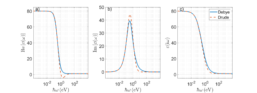
Figure 7: a) Real, b) imaginary parts of the permittivity in Debye und Drude models with $\hbar\omega_{D}=1\,\rm{eV},\varepsilon_{s}=80,\varepsilon_{\infty}=1$. c) Permittivities at imaginary frequencies. The vertical lines indicate $\omega_{D}$.

Drude and Debye approximations are very similar if one identifies $\tau_{D}=\gamma_{D}/\omega_{D}^{2}$ and $\gamma_{D}=3\omega_{D}$ as shown for a simple “water” model with $\hbar\omega_{D}=1\,\rm{eV},\varepsilon_{s}=80,\varepsilon_{\infty}=1$ in Figure 7.

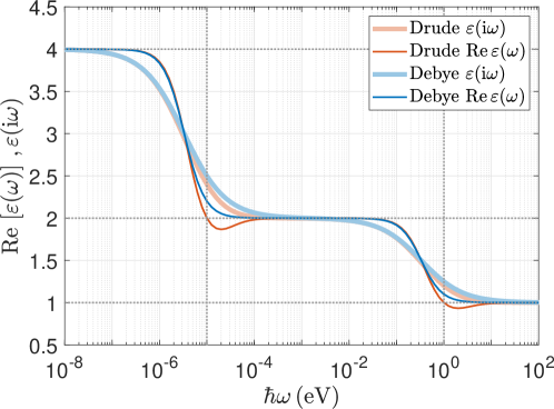
Figure 8: Comparison of the dielectric function on the imaginary frequency axis and the corresponding real part for a two oscillator model with the parameters $\hbar\omega_{D}=\left\{10^{-5},1\right\}\,\rm{eV}$ and $\varepsilon_{D}=\left\{2,1\right\}$.

Figure 8 compares the real part of the dielectric function and the corresponding function at the imaginary frequency axis.

Appendix B Table of medium-assisted Van der Waals interaction of small molecules in different solvents

Table 5: Comparison of different molecule combinations (Molecule A and B) with the vacuum Van der Waals coefficient $C_{6}^{\rm vac}\,(10^{79}\rm{Jm}^{6})$, the corresponding averaged main-frequency $\overline{\omega}\,(\rm{eV})$, the exact and approximated (32) dielectric functions evaluated at the averaged main-frequency, the approximated Van der Waals coefficient according to Eq. (3) $C_{6}^{\rm app}\,(10^{79}\rm{Jm}^{6})$, the exact Van der Waals coefficient according to Eq. (2) $C_{6}^{\rm exact}\,(10^{79}\rm{Jm}^{6})$ and the relative deviation of the approximated and exact $C_{6}$-coefficients.

Mol. A	Medium	Mol. B	$C_{6}^{\rm vac}$	$\overline{\omega}$	$\varepsilon({\rm i}\overline{\omega})$	$\varepsilon_{\rm app}({\rm i}\overline{\omega})$	$C_{6}^{\rm app}$	$C_{6}^{\rm exact}$	rel. Dev.
CH4	Water	CH4	116.68	11.35	1.47	1.46	54.48	51.90	4.99
CH4	Water	NO2	134.21	12.60	1.43	1.43	65.27	61.21	6.63
CH4	Water	CO2	136.68	12.64	1.43	1.43	66.56	62.51	6.48
CH4	Water	CO	96.18	12.15	1.45	1.44	46.13	43.47	6.12
CH4	Water	N2O	147.94	12.34	1.44	1.44	71.38	67.16	6.28
CH4	Water	O3	139.65	12.67	1.43	1.43	68.06	63.74	6.79
CH4	Water	O2	81.51	13.24	1.42	1.42	40.42	37.75	7.07
CH4	Water	N2	90.15	12.76	1.43	1.43	44.06	41.40	6.43
CH4	Water	H2S	157.89	10.28	1.50	1.49	70.96	68.16	4.10
CH4	Water	NO	87.30	12.79	1.43	1.43	42.71	40.05	6.64
NO2	Water	CH4	134.21	12.60	1.43	1.43	65.27	61.21	6.63
NO2	Water	NO2	155.68	14.24	1.40	1.40	79.38	73.17	8.49
NO2	Water	CO2	158.50	14.26	1.40	1.40	80.84	74.66	8.28
NO2	Water	CO	111.21	13.67	1.41	1.41	55.82	51.71	7.95
NO2	Water	N2O	171.27	13.90	1.40	1.41	86.52	80.03	8.11
NO2	Water	O3	162.11	14.35	1.39	1.40	82.90	76.28	8.67
NO2	Water	O2	94.92	15.03	1.38	1.39	49.38	45.37	8.85
NO2	Water	N2	104.61	14.37	1.39	1.40	53.51	49.48	8.16
NO2	Water	H2S	180.42	11.34	1.47	1.46	84.22	79.64	5.74
NO2	Water	NO	101.36	14.45	1.39	1.40	51.97	47.92	8.44
CO2	Water	CH4	136.68	12.64	1.43	1.43	66.56	62.51	6.48
CO2	Water	NO2	158.50	14.26	1.40	1.40	80.84	74.66	8.28
CO2	Water	CO2	161.47	14.27	1.40	1.40	82.38	76.22	8.08
CO2	Water	CO	113.25	13.69	1.41	1.41	56.88	52.78	7.76
CO2	Water	N2O	174.42	13.92	1.40	1.41	88.16	81.69	7.91
CO2	Water	O3	165.01	14.36	1.39	1.40	84.40	77.82	8.46
CO2	Water	O2	96.69	15.03	1.38	1.39	50.30	46.30	8.63
CO2	Water	N2	106.60	14.38	1.39	1.40	54.55	50.53	7.96
CO2	Water	H2S	183.51	11.40	1.47	1.46	85.84	81.27	5.63
CO2	Water	NO	103.25	14.46	1.39	1.40	52.94	48.92	8.23
CO	Water	CH4	96.18	12.15	1.45	1.44	46.13	43.47	6.12
CO	Water	NO2	111.21	13.67	1.41	1.41	55.82	51.71	7.95
CO	Water	CO2	113.25	13.69	1.41	1.41	56.88	52.78	7.76
CO	Water	CO	79.54	13.13	1.42	1.42	39.32	36.61	7.41
CO	Water	N2O	122.44	13.35	1.42	1.42	60.91	56.62	7.57
CO	Water	O3	115.77	13.76	1.41	1.41	58.26	53.88	8.13
CO	Water	O2	67.71	14.41	1.39	1.40	34.67	32.00	8.36
CO	Water	N2	74.72	13.80	1.41	1.41	37.65	34.97	7.66
CO	Water	H2S	129.60	10.96	1.48	1.47	59.71	56.75	5.21
CO	Water	NO	72.38	13.87	1.41	1.41	36.54	33.85	7.93
N2O	Water	CH4	147.94	12.34	1.44	1.44	71.38	67.16	6.28
N2O	Water	NO2	171.27	13.90	1.40	1.41	86.52	80.03	8.11
N2O	Water	CO2	174.42	13.92	1.40	1.41	88.16	81.69	7.91
N2O	Water	CO	122.44	13.35	1.42	1.42	60.91	56.62	7.57
N2O	Water	N2O	188.52	13.58	1.41	1.41	94.38	87.60	7.73
N2O	Water	O3	178.30	14.00	1.40	1.41	90.32	83.41	8.29
N2O	Water	O2	104.35	14.65	1.39	1.39	53.78	49.57	8.49
N2O	Water	N2	115.11	14.03	1.40	1.40	58.36	54.13	7.80
N2O	Water	H2S	199.10	11.13	1.47	1.47	92.26	87.54	5.39
N2O	Water	NO	111.50	14.10	1.40	1.40	56.64	52.41	8.07
O3	Water	CH4	139.65	12.67	1.43	1.43	68.06	63.74	6.79
O3	Water	NO2	162.11	14.35	1.39	1.40	82.90	76.28	8.67
O3	Water	CO2	165.01	14.36	1.39	1.40	84.40	77.82	8.46
O3	Water	CO	115.77	13.76	1.41	1.41	58.26	53.88	8.13
O3	Water	N2O	178.30	14.00	1.40	1.41	90.32	83.41	8.29
O3	Water	O3	168.83	14.47	1.39	1.40	86.59	79.54	8.86
O3	Water	O2	98.84	15.16	1.38	1.38	51.58	47.31	9.02
O3	Water	N2	108.90	14.48	1.39	1.40	55.87	51.57	8.33
O3	Water	H2S	187.75	11.39	1.47	1.46	87.79	82.90	5.89
O3	Water	NO	105.53	14.56	1.39	1.39	54.26	49.96	8.62
O2	Water	CH4	81.51	13.24	1.42	1.42	40.42	37.75	7.07
O2	Water	NO2	94.92	15.03	1.38	1.39	49.38	45.37	8.85
O2	Water	CO2	96.69	15.03	1.38	1.39	50.30	46.30	8.63
O2	Water	CO	67.71	14.41	1.39	1.40	34.67	32.00	8.36
O2	Water	N2O	104.35	14.65	1.39	1.39	53.78	49.57	8.49
O2	Water	O3	98.84	15.16	1.38	1.38	51.58	47.31	9.02
O2	Water	O2	58.01	15.86	1.36	1.37	30.78	28.20	9.12
O2	Water	N2	63.86	15.13	1.38	1.38	33.30	30.70	8.48
O2	Water	H2S	109.06	11.92	1.45	1.45	51.92	48.85	6.27
O2	Water	NO	61.86	15.24	1.38	1.38	32.34	29.74	8.77
N2	Water	CH4	90.15	12.76	1.43	1.43	44.06	41.40	6.43
N2	Water	NO2	104.61	14.37	1.39	1.40	53.51	49.48	8.16
N2	Water	CO2	106.60	14.38	1.39	1.40	54.55	50.53	7.96
N2	Water	CO	74.72	13.80	1.41	1.41	37.65	34.97	7.66
N2	Water	N2O	115.11	14.03	1.40	1.40	58.36	54.13	7.80
N2	Water	O3	108.90	14.48	1.39	1.40	55.87	51.57	8.33
N2	Water	O2	63.86	15.13	1.38	1.38	33.30	30.70	8.48
N2	Water	N2	70.40	14.49	1.39	1.40	36.12	33.50	7.83
N2	Water	H2S	120.86	11.52	1.46	1.46	56.76	53.74	5.61
N2	Water	NO	68.17	14.57	1.39	1.39	35.05	32.43	8.10
H2S	Water	CH4	157.89	10.28	1.50	1.49	70.96	68.16	4.10
H2S	Water	NO2	180.42	11.34	1.47	1.46	84.22	79.64	5.74
H2S	Water	CO2	183.51	11.40	1.47	1.46	85.84	81.27	5.63
H2S	Water	CO	129.60	10.96	1.48	1.47	59.71	56.75	5.21
H2S	Water	N2O	199.10	11.13	1.47	1.47	92.26	87.54	5.39
H2S	Water	O3	187.75	11.39	1.47	1.46	87.79	82.90	5.89
H2S	Water	O2	109.06	11.92	1.45	1.45	51.92	48.85	6.27
H2S	Water	N2	120.86	11.52	1.46	1.46	56.76	53.74	5.61
H2S	Water	H2S	215.59	9.33	1.52	1.52	93.40	90.51	3.19
H2S	Water	NO	117.12	11.53	1.46	1.46	55.02	52.01	5.80
NO	Water	CH4	87.30	12.79	1.43	1.43	42.71	40.05	6.64
NO	Water	NO2	101.36	14.45	1.39	1.40	51.97	47.92	8.44
NO	Water	CO2	103.25	14.46	1.39	1.40	52.94	48.92	8.23
NO	Water	CO	72.38	13.87	1.41	1.41	36.54	33.85	7.93
NO	Water	N2O	111.50	14.10	1.40	1.40	56.64	52.41	8.07
NO	Water	O3	105.53	14.56	1.39	1.39	54.26	49.96	8.62
NO	Water	O2	61.86	15.24	1.38	1.38	32.34	29.74	8.77
NO	Water	N2	68.17	14.57	1.39	1.39	35.05	32.43	8.10
NO	Water	H2S	117.12	11.53	1.46	1.46	55.02	52.01	5.80
NO	Water	NO	66.03	14.66	1.39	1.39	34.03	31.40	8.38
CH4	Ethanol	CH4	116.68	11.35	1.53	1.53	50.16	48.76	2.87
CH4	Ethanol	NO2	134.21	12.60	1.49	1.49	60.59	57.71	4.99
CH4	Ethanol	CO2	136.68	12.64	1.49	1.49	61.81	58.93	4.89
CH4	Ethanol	CO	96.18	12.15	1.50	1.50	42.69	40.93	4.30
CH4	Ethanol	N2O	147.94	12.34	1.50	1.50	66.15	63.27	4.55
CH4	Ethanol	O3	139.65	12.67	1.49	1.49	63.22	60.12	5.16
CH4	Ethanol	O2	81.51	13.24	1.47	1.47	37.70	35.65	5.75
CH4	Ethanol	N2	90.15	12.76	1.48	1.48	40.95	39.04	4.89
CH4	Ethanol	H2S	157.89	10.28	1.56	1.56	64.90	63.85	1.64
CH4	Ethanol	NO	87.30	12.79	1.48	1.48	39.70	37.77	5.11
NO2	Ethanol	CH4	134.21	12.60	1.49	1.49	60.59	57.71	4.99
NO2	Ethanol	NO2	155.68	14.24	1.44	1.44	74.57	69.28	7.64
NO2	Ethanol	CO2	158.50	14.26	1.44	1.44	75.96	70.67	7.48
NO2	Ethanol	CO	111.21	13.67	1.46	1.46	52.22	48.88	6.83
NO2	Ethanol	N2O	171.27	13.90	1.45	1.45	81.08	75.70	7.11
NO2	Ethanol	O3	162.11	14.35	1.44	1.44	77.94	72.26	7.86
NO2	Ethanol	O2	94.92	15.03	1.42	1.43	46.66	43.03	8.44
NO2	Ethanol	N2	104.61	14.37	1.44	1.44	50.32	46.85	7.41
NO2	Ethanol	H2S	180.42	11.34	1.53	1.53	77.52	74.85	3.57
NO2	Ethanol	NO	101.36	14.45	1.44	1.44	48.89	45.39	7.72
CO2	Ethanol	CH4	136.68	12.64	1.49	1.49	61.81	58.93	4.89
CO2	Ethanol	NO2	158.50	14.26	1.44	1.44	75.96	70.67	7.48
CO2	Ethanol	CO2	161.47	14.27	1.44	1.44	77.41	72.13	7.31
CO2	Ethanol	CO	113.25	13.69	1.46	1.46	53.22	49.88	6.69
CO2	Ethanol	N2O	174.42	13.92	1.45	1.45	82.62	77.25	6.95
CO2	Ethanol	O3	165.01	14.36	1.44	1.44	79.36	73.69	7.69
CO2	Ethanol	O2	96.69	15.03	1.42	1.43	47.52	43.90	8.25
CO2	Ethanol	N2	106.60	14.38	1.44	1.44	51.29	47.83	7.24
CO2	Ethanol	H2S	183.51	11.40	1.53	1.52	79.05	76.36	3.52
CO2	Ethanol	NO	103.25	14.46	1.44	1.44	49.82	46.32	7.55
CO	Ethanol	CH4	96.18	12.15	1.50	1.50	42.69	40.93	4.30
CO	Ethanol	NO2	111.21	13.67	1.46	1.46	52.22	48.88	6.83
CO	Ethanol	CO2	113.25	13.69	1.46	1.46	53.22	49.88	6.69
CO	Ethanol	CO	79.54	13.13	1.47	1.47	36.64	34.55	6.04
CO	Ethanol	N2O	122.44	13.35	1.47	1.47	56.85	53.47	6.32
CO	Ethanol	O3	115.77	13.76	1.46	1.46	54.55	50.96	7.04
CO	Ethanol	O2	67.71	14.41	1.44	1.44	32.61	30.30	7.64
CO	Ethanol	N2	74.72	13.80	1.45	1.46	35.25	33.06	6.64
CO	Ethanol	H2S	129.60	10.96	1.54	1.54	54.83	53.27	2.93
CO	Ethanol	NO	72.38	13.87	1.45	1.45	34.23	32.01	6.93
N2O	Ethanol	CH4	147.94	12.34	1.50	1.50	66.15	63.27	4.55
N2O	Ethanol	NO2	171.27	13.90	1.45	1.45	81.08	75.70	7.11
N2O	Ethanol	CO2	174.42	13.92	1.45	1.45	82.62	77.25	6.95
N2O	Ethanol	CO	122.44	13.35	1.47	1.47	56.85	53.47	6.32
N2O	Ethanol	N2O	188.52	13.58	1.46	1.46	88.24	82.78	6.59
N2O	Ethanol	O3	178.30	14.00	1.45	1.45	84.71	78.93	7.32
N2O	Ethanol	O2	104.35	14.65	1.43	1.44	50.67	46.96	7.90
N2O	Ethanol	N2	115.11	14.03	1.45	1.45	54.74	51.21	6.90
N2O	Ethanol	H2S	199.10	11.13	1.53	1.53	84.81	82.21	3.17
N2O	Ethanol	NO	111.50	14.10	1.45	1.45	53.16	49.59	7.19
O3	Ethanol	CH4	139.65	12.67	1.49	1.49	63.22	60.12	5.16
O3	Ethanol	NO2	162.11	14.35	1.44	1.44	77.94	72.26	7.86
O3	Ethanol	CO2	165.01	14.36	1.44	1.44	79.36	73.69	7.69
O3	Ethanol	CO	115.77	13.76	1.46	1.46	54.55	50.96	7.04
O3	Ethanol	N2O	178.30	14.00	1.45	1.45	84.71	78.93	7.32
O3	Ethanol	O3	168.83	14.47	1.44	1.44	81.48	75.38	8.09
O3	Ethanol	O2	98.84	15.16	1.42	1.42	48.78	44.89	8.67
O3	Ethanol	N2	108.90	14.48	1.44	1.44	52.57	48.85	7.62
O3	Ethanol	H2S	187.75	11.39	1.53	1.52	80.83	77.94	3.71
O3	Ethanol	NO	105.53	14.56	1.43	1.44	51.10	47.34	7.94
O2	Ethanol	CH4	81.51	13.24	1.47	1.47	37.70	35.65	5.75
O2	Ethanol	NO2	94.92	15.03	1.42	1.43	46.66	43.03	8.44
O2	Ethanol	CO2	96.69	15.03	1.42	1.43	47.52	43.90	8.25
O2	Ethanol	CO	67.71	14.41	1.44	1.44	32.61	30.30	7.64
O2	Ethanol	N2O	104.35	14.65	1.43	1.44	50.67	46.96	7.90
O2	Ethanol	O3	98.84	15.16	1.42	1.42	48.78	44.89	8.67
O2	Ethanol	O2	58.01	15.86	1.40	1.41	29.26	26.80	9.18
O2	Ethanol	N2	63.86	15.13	1.42	1.42	31.49	29.12	8.15
O2	Ethanol	H2S	109.06	11.92	1.51	1.51	47.97	45.97	4.35
O2	Ethanol	NO	61.86	15.24	1.42	1.42	30.61	28.21	8.49
N2	Ethanol	CH4	90.15	12.76	1.48	1.48	40.95	39.04	4.89
N2	Ethanol	NO2	104.61	14.37	1.44	1.44	50.32	46.85	7.41
N2	Ethanol	CO2	106.60	14.38	1.44	1.44	51.29	47.83	7.24
N2	Ethanol	CO	74.72	13.80	1.45	1.46	35.25	33.06	6.64
N2	Ethanol	N2O	115.11	14.03	1.45	1.45	54.74	51.21	6.90
N2	Ethanol	O3	108.90	14.48	1.44	1.44	52.57	48.85	7.62
N2	Ethanol	O2	63.86	15.13	1.42	1.42	31.49	29.12	8.15
N2	Ethanol	N2	70.40	14.49	1.44	1.44	34.00	31.72	7.17
N2	Ethanol	H2S	120.86	11.52	1.52	1.52	52.30	50.51	3.55
N2	Ethanol	NO	68.17	14.57	1.43	1.44	33.01	30.72	7.47
H2S	Ethanol	CH4	157.89	10.28	1.56	1.56	64.90	63.85	1.64
H2S	Ethanol	NO2	180.42	11.34	1.53	1.53	77.52	74.85	3.57
H2S	Ethanol	CO2	183.51	11.40	1.53	1.52	79.05	76.36	3.52
H2S	Ethanol	CO	129.60	10.96	1.54	1.54	54.83	53.27	2.93
H2S	Ethanol	N2O	199.10	11.13	1.53	1.53	84.81	82.21	3.17
H2S	Ethanol	O3	187.75	11.39	1.53	1.52	80.83	77.94	3.71
H2S	Ethanol	O2	109.06	11.92	1.51	1.51	47.97	45.97	4.35
H2S	Ethanol	N2	120.86	11.52	1.52	1.52	52.30	50.51	3.55
H2S	Ethanol	H2S	215.59	9.33	1.59	1.59	84.99	84.56	0.50
H2S	Ethanol	NO	117.12	11.53	1.52	1.52	50.71	48.89	3.72
NO	Ethanol	CH4	87.30	12.79	1.48	1.48	39.70	37.77	5.11
NO	Ethanol	NO2	101.36	14.45	1.44	1.44	48.89	45.39	7.72
NO	Ethanol	CO2	103.25	14.46	1.44	1.44	49.82	46.32	7.55
NO	Ethanol	CO	72.38	13.87	1.45	1.45	34.23	32.01	6.93
NO	Ethanol	N2O	111.50	14.10	1.45	1.45	53.16	49.59	7.19
NO	Ethanol	O3	105.53	14.56	1.43	1.44	51.10	47.34	7.94
NO	Ethanol	O2	61.86	15.24	1.42	1.42	30.61	28.21	8.49
NO	Ethanol	N2	68.17	14.57	1.43	1.44	33.01	30.72	7.47
NO	Ethanol	H2S	117.12	11.53	1.52	1.52	50.71	48.89	3.72
NO	Ethanol	NO	66.03	14.66	1.43	1.43	32.07	29.75	7.79
CH4	Methanol	CH4	116.68	11.35	1.46	1.46	54.52	52.41	4.04
CH4	Methanol	NO2	134.21	12.60	1.43	1.43	65.79	61.87	6.33
CH4	Methanol	CO2	136.68	12.64	1.43	1.43	67.11	63.18	6.22
CH4	Methanol	CO	96.18	12.15	1.44	1.44	46.37	43.92	5.58
CH4	Methanol	N2O	147.94	12.34	1.43	1.44	71.84	67.87	5.85
CH4	Methanol	O3	139.65	12.67	1.43	1.43	68.64	64.44	6.52
CH4	Methanol	O2	81.51	13.24	1.41	1.41	40.91	38.18	7.16
CH4	Methanol	N2	90.15	12.76	1.42	1.42	44.45	41.85	6.22
CH4	Methanol	H2S	157.89	10.28	1.49	1.50	70.63	68.76	2.71
CH4	Methanol	NO	87.30	12.79	1.42	1.42	43.10	40.49	6.46
NO2	Methanol	CH4	134.21	12.60	1.43	1.43	65.79	61.87	6.33
NO2	Methanol	NO2	155.68	14.24	1.39	1.39	80.87	74.04	9.22
NO2	Methanol	CO2	158.50	14.26	1.39	1.39	82.37	75.55	9.03
NO2	Methanol	CO	111.21	13.67	1.40	1.40	56.65	52.30	8.32
NO2	Methanol	N2O	171.27	13.90	1.40	1.40	87.95	80.97	8.62
NO2	Methanol	O3	162.11	14.35	1.38	1.38	84.52	77.20	9.47
NO2	Methanol	O2	94.92	15.03	1.37	1.37	50.57	45.93	10.11
NO2	Methanol	N2	104.61	14.37	1.38	1.38	54.57	50.07	8.97
NO2	Methanol	H2S	180.42	11.34	1.46	1.46	84.27	80.42	4.78
NO2	Methanol	NO	101.36	14.45	1.38	1.38	53.02	48.50	9.31
CO2	Methanol	CH4	136.68	12.64	1.43	1.43	67.11	63.18	6.22
CO2	Methanol	NO2	158.50	14.26	1.39	1.39	82.37	75.55	9.03
CO2	Methanol	CO2	161.47	14.27	1.39	1.39	83.94	77.13	8.84
CO2	Methanol	CO	113.25	13.69	1.40	1.40	57.73	53.38	8.15
CO2	Methanol	N2O	174.42	13.92	1.40	1.40	89.62	82.64	8.45
CO2	Methanol	O3	165.01	14.36	1.38	1.38	86.06	78.75	9.28
CO2	Methanol	O2	96.69	15.03	1.37	1.37	51.51	46.88	9.89
CO2	Methanol	N2	106.60	14.38	1.38	1.38	55.62	51.13	8.78
CO2	Methanol	H2S	183.51	11.40	1.46	1.46	85.93	82.06	4.71
CO2	Methanol	NO	103.25	14.46	1.38	1.38	54.02	49.50	9.11
CO	Methanol	CH4	96.18	12.15	1.44	1.44	46.37	43.92	5.58
CO	Methanol	NO2	111.21	13.67	1.40	1.40	56.65	52.30	8.32
CO	Methanol	CO2	113.25	13.69	1.40	1.40	57.73	53.38	8.15
CO	Methanol	CO	79.54	13.13	1.41	1.41	39.77	37.01	7.45
CO	Methanol	N2O	122.44	13.35	1.41	1.41	61.69	57.26	7.75
CO	Methanol	O3	115.77	13.76	1.40	1.40	59.17	54.51	8.55
CO	Methanol	O2	67.71	14.41	1.38	1.38	35.36	32.38	9.21
CO	Methanol	N2	74.72	13.80	1.40	1.40	38.24	35.37	8.11
CO	Methanol	H2S	129.60	10.96	1.47	1.47	59.63	57.29	4.09
CO	Methanol	NO	72.38	13.87	1.40	1.40	37.13	34.25	8.42
N2O	Methanol	CH4	147.94	12.34	1.43	1.44	71.84	67.87	5.85
N2O	Methanol	NO2	171.27	13.90	1.40	1.40	87.95	80.97	8.62
N2O	Methanol	CO2	174.42	13.92	1.40	1.40	89.62	82.64	8.45
N2O	Methanol	CO	122.44	13.35	1.41	1.41	61.69	57.26	7.75
N2O	Methanol	N2O	188.52	13.58	1.40	1.40	95.73	88.60	8.05
N2O	Methanol	O3	178.30	14.00	1.39	1.39	91.88	84.39	8.87
N2O	Methanol	O2	104.35	14.65	1.38	1.38	54.94	50.17	9.51
N2O	Methanol	N2	115.11	14.03	1.39	1.39	59.37	54.77	8.40
N2O	Methanol	H2S	199.10	11.13	1.47	1.47	92.22	88.38	4.34
N2O	Methanol	NO	111.50	14.10	1.39	1.39	57.65	53.03	8.72
O3	Methanol	CH4	139.65	12.67	1.43	1.43	68.64	64.44	6.52
O3	Methanol	NO2	162.11	14.35	1.38	1.38	84.52	77.20	9.47
O3	Methanol	CO2	165.01	14.36	1.38	1.38	86.06	78.75	9.28
O3	Methanol	CO	115.77	13.76	1.40	1.40	59.17	54.51	8.55
O3	Methanol	N2O	178.30	14.00	1.39	1.39	91.88	84.39	8.87
O3	Methanol	O3	168.83	14.47	1.38	1.38	88.35	80.51	9.73
O3	Methanol	O2	98.84	15.16	1.37	1.37	52.87	47.90	10.37
O3	Methanol	N2	108.90	14.48	1.38	1.38	57.01	52.20	9.21
O3	Methanol	H2S	187.75	11.39	1.46	1.46	87.87	83.73	4.94
O3	Methanol	NO	105.53	14.56	1.38	1.38	55.40	50.57	9.56
O2	Methanol	CH4	81.51	13.24	1.41	1.41	40.91	38.18	7.16
O2	Methanol	NO2	94.92	15.03	1.37	1.37	50.57	45.93	10.11
O2	Methanol	CO2	96.69	15.03	1.37	1.37	51.51	46.88	9.89
O2	Methanol	CO	67.71	14.41	1.38	1.38	35.36	32.38	9.21
O2	Methanol	N2O	104.35	14.65	1.38	1.38	54.94	50.17	9.51
O2	Methanol	O3	98.84	15.16	1.37	1.37	52.87	47.90	10.37
O2	Methanol	O2	58.01	15.86	1.35	1.35	31.70	28.57	10.94
O2	Methanol	N2	63.86	15.13	1.37	1.37	34.13	31.09	9.80
O2	Methanol	H2S	109.06	11.92	1.45	1.45	52.12	49.35	5.61
O2	Methanol	NO	61.86	15.24	1.36	1.37	33.17	30.11	10.17
N2	Methanol	CH4	90.15	12.76	1.42	1.42	44.45	41.85	6.22
N2	Methanol	NO2	104.61	14.37	1.38	1.38	54.57	50.07	8.97
N2	Methanol	CO2	106.60	14.38	1.38	1.38	55.62	51.13	8.78
N2	Methanol	CO	74.72	13.80	1.40	1.40	38.24	35.37	8.11
N2	Methanol	N2O	115.11	14.03	1.39	1.39	59.37	54.77	8.40
N2	Methanol	O3	108.90	14.48	1.38	1.38	57.01	52.20	9.21
N2	Methanol	O2	63.86	15.13	1.37	1.37	34.13	31.09	9.80
N2	Methanol	N2	70.40	14.49	1.38	1.38	36.86	33.91	8.72
N2	Methanol	H2S	120.86	11.52	1.46	1.46	56.85	54.27	4.75
N2	Methanol	NO	68.17	14.57	1.38	1.38	35.79	32.82	9.05
H2S	Methanol	CH4	157.89	10.28	1.49	1.50	70.63	68.76	2.71
H2S	Methanol	NO2	180.42	11.34	1.46	1.46	84.27	80.42	4.78
H2S	Methanol	CO2	183.51	11.40	1.46	1.46	85.93	82.06	4.71
H2S	Methanol	CO	129.60	10.96	1.47	1.47	59.63	57.29	4.09
H2S	Methanol	N2O	199.10	11.13	1.47	1.47	92.22	88.38	4.34
H2S	Methanol	O3	187.75	11.39	1.46	1.46	87.87	83.73	4.94
H2S	Methanol	O2	109.06	11.92	1.45	1.45	52.12	49.35	5.61
H2S	Methanol	N2	120.86	11.52	1.46	1.46	56.85	54.27	4.75
H2S	Methanol	H2S	215.59	9.33	1.52	1.53	92.60	91.23	1.50
H2S	Methanol	NO	117.12	11.53	1.46	1.46	55.11	52.52	4.94
NO	Methanol	CH4	87.30	12.79	1.42	1.42	43.10	40.49	6.46
NO	Methanol	NO2	101.36	14.45	1.38	1.38	53.02	48.50	9.31
NO	Methanol	CO2	103.25	14.46	1.38	1.38	54.02	49.50	9.11
NO	Methanol	CO	72.38	13.87	1.40	1.40	37.13	34.25	8.42
NO	Methanol	N2O	111.50	14.10	1.39	1.39	57.65	53.03	8.72
NO	Methanol	O3	105.53	14.56	1.38	1.38	55.40	50.57	9.56
NO	Methanol	O2	61.86	15.24	1.36	1.37	33.17	30.11	10.17
NO	Methanol	N2	68.17	14.57	1.38	1.38	35.79	32.82	9.05
NO	Methanol	H2S	117.12	11.53	1.46	1.46	55.11	52.52	4.94
NO	Methanol	NO	66.03	14.66	1.38	1.38	34.77	31.78	9.39
CH4	Butanol	CH4	116.68	11.35	1.56	1.56	48.06	46.41	3.56
CH4	Butanol	NO2	134.21	12.60	1.52	1.52	58.34	55.10	5.89
CH4	Butanol	CO2	136.68	12.64	1.52	1.52	59.53	56.27	5.78
CH4	Butanol	CO	96.18	12.15	1.53	1.53	41.04	39.03	5.15
CH4	Butanol	N2O	147.94	12.34	1.53	1.52	63.63	60.36	5.41
CH4	Butanol	O3	139.65	12.67	1.52	1.51	60.89	57.40	6.08
CH4	Butanol	O2	81.51	13.24	1.50	1.50	36.38	34.09	6.71
CH4	Butanol	N2	90.15	12.76	1.51	1.51	39.45	37.30	5.77
CH4	Butanol	H2S	157.89	10.28	1.60	1.60	61.87	60.55	2.18
CH4	Butanol	NO	87.30	12.79	1.51	1.51	38.26	36.09	6.02
NO2	Butanol	CH4	134.21	12.60	1.52	1.52	58.34	55.10	5.89
NO2	Butanol	NO2	155.68	14.24	1.47	1.47	72.17	66.36	8.76
NO2	Butanol	CO2	158.50	14.26	1.47	1.47	73.51	67.71	8.57
NO2	Butanol	CO	111.21	13.67	1.48	1.48	50.46	46.77	7.89
NO2	Butanol	N2O	171.27	13.90	1.48	1.48	78.40	72.46	8.18
NO2	Butanol	O3	162.11	14.35	1.46	1.47	75.45	69.22	9.00
NO2	Butanol	O2	94.92	15.03	1.44	1.45	45.24	41.29	9.58
NO2	Butanol	N2	104.61	14.37	1.46	1.47	48.72	44.91	8.48
NO2	Butanol	H2S	180.42	11.34	1.56	1.56	74.27	71.18	4.35
NO2	Butanol	NO	101.36	14.45	1.46	1.46	47.35	43.51	8.83
CO2	Butanol	CH4	136.68	12.64	1.52	1.52	59.53	56.27	5.78
CO2	Butanol	NO2	158.50	14.26	1.47	1.47	73.51	67.71	8.57
CO2	Butanol	CO2	161.47	14.27	1.47	1.47	74.92	69.13	8.38
CO2	Butanol	CO	113.25	13.69	1.48	1.48	51.42	47.74	7.73
CO2	Butanol	N2O	174.42	13.92	1.48	1.48	79.89	73.97	8.01
CO2	Butanol	O3	165.01	14.36	1.46	1.47	76.83	70.61	8.80
CO2	Butanol	O2	96.69	15.03	1.44	1.45	46.08	42.14	9.36
CO2	Butanol	N2	106.60	14.38	1.46	1.47	49.66	45.86	8.29
CO2	Butanol	H2S	183.51	11.40	1.56	1.56	75.76	72.64	4.29
CO2	Butanol	NO	103.25	14.46	1.46	1.46	48.24	44.41	8.63
CO	Butanol	CH4	96.18	12.15	1.53	1.53	41.04	39.03	5.15
CO	Butanol	NO2	111.21	13.67	1.48	1.48	50.46	46.77	7.89
CO	Butanol	CO2	113.25	13.69	1.48	1.48	51.42	47.74	7.73
CO	Butanol	CO	79.54	13.13	1.50	1.50	35.35	33.02	7.05
CO	Butanol	N2O	122.44	13.35	1.49	1.49	54.88	51.13	7.34
CO	Butanol	O3	115.77	13.76	1.48	1.48	52.72	48.76	8.13
CO	Butanol	O2	67.71	14.41	1.46	1.46	31.58	29.04	8.73
CO	Butanol	N2	74.72	13.80	1.48	1.48	34.08	31.65	7.66
CO	Butanol	H2S	129.60	10.96	1.57	1.57	52.45	50.60	3.64
CO	Butanol	NO	72.38	13.87	1.48	1.48	33.10	30.65	7.98
N2O	Butanol	CH4	147.94	12.34	1.53	1.52	63.63	60.36	5.41
N2O	Butanol	NO2	171.27	13.90	1.48	1.48	78.40	72.46	8.18
N2O	Butanol	CO2	174.42	13.92	1.48	1.48	79.89	73.97	8.01
N2O	Butanol	CO	122.44	13.35	1.49	1.49	54.88	51.13	7.34
N2O	Butanol	N2O	188.52	13.58	1.49	1.49	85.23	79.19	7.63
N2O	Butanol	O3	178.30	14.00	1.47	1.48	81.92	75.56	8.42
N2O	Butanol	O2	104.35	14.65	1.45	1.46	49.09	45.04	9.01
N2O	Butanol	N2	115.11	14.03	1.47	1.47	52.95	49.05	7.93
N2O	Butanol	H2S	199.10	11.13	1.57	1.57	81.18	78.13	3.90
N2O	Butanol	NO	111.50	14.10	1.47	1.47	51.43	47.50	8.26
O3	Butanol	CH4	139.65	12.67	1.52	1.51	60.89	57.40	6.08
O3	Butanol	NO2	162.11	14.35	1.46	1.47	75.45	69.22	9.00
O3	Butanol	CO2	165.01	14.36	1.46	1.47	76.83	70.61	8.80
O3	Butanol	CO	115.77	13.76	1.48	1.48	52.72	48.76	8.13
O3	Butanol	N2O	178.30	14.00	1.47	1.48	81.92	75.56	8.42
O3	Butanol	O3	168.83	14.47	1.46	1.46	78.90	72.22	9.25
O3	Butanol	O2	98.84	15.16	1.44	1.45	47.32	43.08	9.82
O3	Butanol	N2	108.90	14.48	1.46	1.46	50.91	46.83	8.71
O3	Butanol	H2S	187.75	11.39	1.56	1.56	77.46	74.12	4.51
O3	Butanol	NO	105.53	14.56	1.46	1.46	49.49	45.38	9.07
O2	Butanol	CH4	81.51	13.24	1.50	1.50	36.38	34.09	6.71
O2	Butanol	NO2	94.92	15.03	1.44	1.45	45.24	41.29	9.58
O2	Butanol	CO2	96.69	15.03	1.44	1.45	46.08	42.14	9.36
O2	Butanol	CO	67.71	14.41	1.46	1.46	31.58	29.04	8.73
O2	Butanol	N2O	104.35	14.65	1.45	1.46	49.09	45.04	9.01
O2	Butanol	O3	98.84	15.16	1.44	1.45	47.32	43.08	9.82
O2	Butanol	O2	58.01	15.86	1.42	1.43	28.42	25.76	10.31
O2	Butanol	N2	63.86	15.13	1.44	1.45	30.55	27.96	9.24
O2	Butanol	H2S	109.06	11.92	1.54	1.54	46.08	43.79	5.21
O2	Butanol	NO	61.86	15.24	1.44	1.44	29.69	27.09	9.61
N2	Butanol	CH4	90.15	12.76	1.51	1.51	39.45	37.30	5.77
N2	Butanol	NO2	104.61	14.37	1.46	1.47	48.72	44.91	8.48
N2	Butanol	CO2	106.60	14.38	1.46	1.47	49.66	45.86	8.29
N2	Butanol	CO	74.72	13.80	1.48	1.48	34.08	31.65	7.66
N2	Butanol	N2O	115.11	14.03	1.47	1.47	52.95	49.05	7.93
N2	Butanol	O3	108.90	14.48	1.46	1.46	50.91	46.83	8.71
N2	Butanol	O2	63.86	15.13	1.44	1.45	30.55	27.96	9.24
N2	Butanol	N2	70.40	14.49	1.46	1.46	32.92	30.43	8.20
N2	Butanol	H2S	120.86	11.52	1.55	1.55	50.15	48.08	4.32
N2	Butanol	NO	68.17	14.57	1.46	1.46	31.97	29.46	8.53
H2S	Butanol	CH4	157.89	10.28	1.60	1.60	61.87	60.55	2.18
H2S	Butanol	NO2	180.42	11.34	1.56	1.56	74.27	71.18	4.35
H2S	Butanol	CO2	183.51	11.40	1.56	1.56	75.76	72.64	4.29
H2S	Butanol	CO	129.60	10.96	1.57	1.57	52.45	50.60	3.64
H2S	Butanol	N2O	199.10	11.13	1.57	1.57	81.18	78.13	3.90
H2S	Butanol	O3	187.75	11.39	1.56	1.56	77.46	74.12	4.51
H2S	Butanol	O2	109.06	11.92	1.54	1.54	46.08	43.79	5.21
H2S	Butanol	N2	120.86	11.52	1.55	1.55	50.15	48.08	4.32
H2S	Butanol	H2S	215.59	9.33	1.64	1.64	80.60	79.90	0.87
H2S	Butanol	NO	117.12	11.53	1.55	1.55	48.62	46.52	4.52
NO	Butanol	CH4	87.30	12.79	1.51	1.51	38.26	36.09	6.02
NO	Butanol	NO2	101.36	14.45	1.46	1.46	47.35	43.51	8.83
NO	Butanol	CO2	103.25	14.46	1.46	1.46	48.24	44.41	8.63
NO	Butanol	CO	72.38	13.87	1.48	1.48	33.10	30.65	7.98
NO	Butanol	N2O	111.50	14.10	1.47	1.47	51.43	47.50	8.26
NO	Butanol	O3	105.53	14.56	1.46	1.46	49.49	45.38	9.07
NO	Butanol	O2	61.86	15.24	1.44	1.44	29.69	27.09	9.61
NO	Butanol	N2	68.17	14.57	1.46	1.46	31.97	29.46	8.53
NO	Butanol	H2S	117.12	11.53	1.55	1.55	48.62	46.52	4.52
NO	Butanol	NO	66.03	14.66	1.45	1.46	31.07	28.53	8.88
CH4	Propanol	CH4	116.68	11.35	1.54	1.54	49.31	47.35	4.14
CH4	Propanol	NO2	134.21	12.60	1.50	1.50	59.81	56.16	6.50
CH4	Propanol	CO2	136.68	12.64	1.50	1.50	61.02	57.36	6.38
CH4	Propanol	CO	96.18	12.15	1.51	1.51	42.08	39.80	5.74
CH4	Propanol	N2O	147.94	12.34	1.51	1.51	65.25	61.54	6.01
CH4	Propanol	O3	139.65	12.67	1.50	1.50	62.42	58.50	6.70
CH4	Propanol	O2	81.51	13.24	1.48	1.48	37.28	34.74	7.32
CH4	Propanol	N2	90.15	12.76	1.49	1.49	40.44	38.02	6.37
CH4	Propanol	H2S	157.89	10.28	1.58	1.58	63.53	61.82	2.76
CH4	Propanol	NO	87.30	12.79	1.49	1.49	39.22	36.78	6.62
NO2	Propanol	CH4	134.21	12.60	1.50	1.50	59.81	56.16	6.50
NO2	Propanol	NO2	155.68	14.24	1.45	1.45	73.92	67.57	9.40
NO2	Propanol	CO2	158.50	14.26	1.45	1.45	75.29	68.95	9.19
NO2	Propanol	CO	111.21	13.67	1.47	1.47	51.69	47.64	8.52
NO2	Propanol	N2O	171.27	13.90	1.46	1.46	80.31	73.80	8.81
NO2	Propanol	O3	162.11	14.35	1.45	1.45	77.27	70.47	9.65
NO2	Propanol	O2	94.92	15.03	1.43	1.43	46.32	42.02	10.22
NO2	Propanol	N2	104.61	14.37	1.45	1.45	49.89	45.73	9.10
NO2	Propanol	H2S	180.42	11.34	1.54	1.54	76.21	72.61	4.96
NO2	Propanol	NO	101.36	14.45	1.44	1.45	48.48	44.29	9.46
CO2	Propanol	CH4	136.68	12.64	1.50	1.50	61.02	57.36	6.38
CO2	Propanol	NO2	158.50	14.26	1.45	1.45	75.29	68.95	9.19
CO2	Propanol	CO2	161.47	14.27	1.45	1.45	76.73	70.40	8.99
CO2	Propanol	CO	113.25	13.69	1.47	1.47	52.68	48.63	8.34
CO2	Propanol	N2O	174.42	13.92	1.46	1.46	81.84	75.34	8.62
CO2	Propanol	O3	165.01	14.36	1.45	1.45	78.68	71.90	9.44
CO2	Propanol	O2	96.69	15.03	1.43	1.43	47.18	42.89	9.99
CO2	Propanol	N2	106.60	14.38	1.45	1.45	50.86	46.70	8.90
CO2	Propanol	H2S	183.51	11.40	1.54	1.54	77.73	74.11	4.88
CO2	Propanol	NO	103.25	14.46	1.44	1.45	49.40	45.22	9.25
CO	Propanol	CH4	96.18	12.15	1.51	1.51	42.08	39.80	5.74
CO	Propanol	NO2	111.21	13.67	1.47	1.47	51.69	47.64	8.52
CO	Propanol	CO2	113.25	13.69	1.47	1.47	52.68	48.63	8.34
CO	Propanol	CO	79.54	13.13	1.48	1.48	36.22	33.65	7.66
CO	Propanol	N2O	122.44	13.35	1.48	1.48	56.24	52.09	7.95
CO	Propanol	O3	115.77	13.76	1.46	1.46	54.01	49.66	8.76
CO	Propanol	O2	67.71	14.41	1.44	1.45	32.34	29.57	9.36
CO	Propanol	N2	74.72	13.80	1.46	1.46	34.91	32.24	8.27
CO	Propanol	H2S	129.60	10.96	1.55	1.55	53.83	51.64	4.23
CO	Propanol	NO	72.38	13.87	1.46	1.46	33.90	31.22	8.60
N2O	Propanol	CH4	147.94	12.34	1.51	1.51	65.25	61.54	6.01
N2O	Propanol	NO2	171.27	13.90	1.46	1.46	80.31	73.80	8.81
N2O	Propanol	CO2	174.42	13.92	1.46	1.46	81.84	75.34	8.62
N2O	Propanol	CO	122.44	13.35	1.48	1.48	56.24	52.09	7.95
N2O	Propanol	N2O	188.52	13.58	1.47	1.47	87.33	80.68	8.24
N2O	Propanol	O3	178.30	14.00	1.46	1.46	83.92	76.95	9.05
N2O	Propanol	O2	104.35	14.65	1.44	1.44	50.27	45.85	9.64
N2O	Propanol	N2	115.11	14.03	1.46	1.46	54.23	49.96	8.55
N2O	Propanol	H2S	199.10	11.13	1.55	1.55	83.31	79.73	4.50
N2O	Propanol	NO	111.50	14.10	1.45	1.45	52.67	48.38	8.89
O3	Propanol	CH4	139.65	12.67	1.50	1.50	62.42	58.50	6.70
O3	Propanol	NO2	162.11	14.35	1.45	1.45	77.27	70.47	9.65
O3	Propanol	CO2	165.01	14.36	1.45	1.45	78.68	71.90	9.44
O3	Propanol	CO	115.77	13.76	1.46	1.46	54.01	49.66	8.76
O3	Propanol	N2O	178.30	14.00	1.46	1.46	83.92	76.95	9.05
O3	Propanol	O3	168.83	14.47	1.44	1.45	80.80	73.52	9.90
O3	Propanol	O2	98.84	15.16	1.42	1.43	48.44	43.84	10.47
O3	Propanol	N2	108.90	14.48	1.44	1.45	52.13	47.68	9.34
O3	Propanol	H2S	187.75	11.39	1.54	1.54	79.48	75.61	5.12
O3	Propanol	NO	105.53	14.56	1.44	1.44	50.68	46.20	9.71
O2	Propanol	CH4	81.51	13.24	1.48	1.48	37.28	34.74	7.32
O2	Propanol	NO2	94.92	15.03	1.43	1.43	46.32	42.02	10.22
O2	Propanol	CO2	96.69	15.03	1.43	1.43	47.18	42.89	9.99
O2	Propanol	CO	67.71	14.41	1.44	1.45	32.34	29.57	9.36
O2	Propanol	N2O	104.35	14.65	1.44	1.44	50.27	45.85	9.64
O2	Propanol	O3	98.84	15.16	1.42	1.43	48.44	43.84	10.47
O2	Propanol	O2	58.01	15.86	1.41	1.41	29.08	26.21	10.96
O2	Propanol	N2	63.86	15.13	1.43	1.43	31.27	28.46	9.87
O2	Propanol	H2S	109.06	11.92	1.52	1.52	47.26	44.66	5.81
O2	Propanol	NO	61.86	15.24	1.42	1.43	30.40	27.57	10.24
N2	Propanol	CH4	90.15	12.76	1.49	1.49	40.44	38.02	6.37
N2	Propanol	NO2	104.61	14.37	1.45	1.45	49.89	45.73	9.10
N2	Propanol	CO2	106.60	14.38	1.45	1.45	50.86	46.70	8.90
N2	Propanol	CO	74.72	13.80	1.46	1.46	34.91	32.24	8.27
N2	Propanol	N2O	115.11	14.03	1.46	1.46	54.23	49.96	8.55
N2	Propanol	O3	108.90	14.48	1.44	1.45	52.13	47.68	9.34
N2	Propanol	O2	63.86	15.13	1.43	1.43	31.27	28.46	9.87
N2	Propanol	N2	70.40	14.49	1.44	1.44	33.71	30.98	8.82
N2	Propanol	H2S	120.86	11.52	1.53	1.53	51.45	49.05	4.91
N2	Propanol	NO	68.17	14.57	1.44	1.44	32.74	30.00	9.16
H2S	Propanol	CH4	157.89	10.28	1.58	1.58	63.53	61.82	2.76
H2S	Propanol	NO2	180.42	11.34	1.54	1.54	76.21	72.61	4.96
H2S	Propanol	CO2	183.51	11.40	1.54	1.54	77.73	74.11	4.88
H2S	Propanol	CO	129.60	10.96	1.55	1.55	53.83	51.64	4.23
H2S	Propanol	N2O	199.10	11.13	1.55	1.55	83.31	79.73	4.50
H2S	Propanol	O3	187.75	11.39	1.54	1.54	79.48	75.61	5.12
H2S	Propanol	O2	109.06	11.92	1.52	1.52	47.26	44.66	5.81
H2S	Propanol	N2	120.86	11.52	1.53	1.53	51.45	49.05	4.91
H2S	Propanol	H2S	215.59	9.33	1.61	1.61	82.84	81.64	1.47
H2S	Propanol	NO	117.12	11.53	1.53	1.53	49.89	47.46	5.12
NO	Propanol	CH4	87.30	12.79	1.49	1.49	39.22	36.78	6.62
NO	Propanol	NO2	101.36	14.45	1.44	1.45	48.48	44.29	9.46
NO	Propanol	CO2	103.25	14.46	1.44	1.45	49.40	45.22	9.25
NO	Propanol	CO	72.38	13.87	1.46	1.46	33.90	31.22	8.60
NO	Propanol	N2O	111.50	14.10	1.45	1.45	52.67	48.38	8.89
NO	Propanol	O3	105.53	14.56	1.44	1.44	50.68	46.20	9.71
NO	Propanol	O2	61.86	15.24	1.42	1.43	30.40	27.57	10.24
NO	Propanol	N2	68.17	14.57	1.44	1.44	32.74	30.00	9.16
NO	Propanol	H2S	117.12	11.53	1.53	1.53	49.89	47.46	5.12
NO	Propanol	NO	66.03	14.66	1.44	1.44	31.81	29.05	9.51

References

- [1] F London. The general theory of molecular forces. J. Chem. Soc. Faraday Trans, 33(8):8b, 1937.
- [2] Johannes Diderik van der Waals. Over de Continuiteit van den Gas- en Vloeistoftoestand [On the continuity of the gas and liquid state]. Ph.d. thesis, University of Leiden, 1873.
- [3] F. London. Zur Theorie und Systematik der Molekularkräfte. Z. Phys., 63(3-4):245–279, mar 1930.
- [4] Kellar Autumn, Yiching A Liang, S Tonia Hsieh, Wolfgang Zesch, Wai Pang Chan, Thomas W Kenny, Ronald Fearing, and Robert J Full. Adhesive force of a single gecko foot-hair. Nature, 405(6787):681–685, 2000.
- [5] Frank W DelRio, Maarten P de Boer, James A Knapp, E David Reedy, Peggy J Clews, and Martin L Dunn. The role of van der Waals forces in adhesion of micromachined surfaces. Nature Mat., 4(8):629–634, 2005.
- [6] R. E. Grisenti, W. Schöllkopf, J. P. Toennies, G. C. Hegerfeldt, and T. Köhler. Determination of Atom-Surface Van der Waals Potentials from Transmission-Grating Diffraction Intensities. Phys. Rev. Lett., 83:1755–1758, 1999.
- [7] M. Arndt, O. Nairz, J. Vos-Andreae, C. Keller, G. van der Zouw, and A. Zeilinger. Wave-particle duality of C60 molecules. Nature, 401(6754):680–682, 1999.
- [8] T. Juffmann, A. Milic, M. Müllneritsch, P. Asenbaum, A. Tsukernik, J. Tüxen, M. Mayor, O. Cheshnovsky, and M. Arndt. Real-time single-molecule imaging of quantum interference. Nature Nanotechn., 7:297 – 300, 2012.
- [9] C. Brand, J. Fiedler, T. Juffmann, M. Sclafani, C. Knobloch, S. Scheel, Y. Lilach, O. Cheshnovsky, and M. Arndt. A Green’s function approach to modeling molecular diffraction in the limit of ultra-thin gratings. Ann. Phys. (Berlin), 527:580–591, 2015.
- [10] H. B. G. Casimir and D. Polder. The influence of retardation on the london-van der waals forces. Phys. Rev., 73:360–372, Feb 1948.
- [11] I. E. Dzyaloshinskii, E. M. Lifshitz, and Lev P. Pitaevskii. General theory of van der waals’ forces. Soviet Physics Uspekhi, 4(2):153, 1961.
- [12] S. Scheel and S. Buhmann. Macroscopic quantum electrodynamics - concepts and applications. Act. Phys. Slov., 58(5), 2008.
- [13] S. Y. Buhmann. Dispersion Forces I: Macroscopic quantum electrodynamics and ground-state Casimir, Casimir–Polder and van der Waals forces. Springer, Heidelberg, 2012.
- [14] A. D. McLachlan. Retarded dispersion forces between molecules. Proc. R. Soc. A., 271(1346):387–401, 1963.
- [15] Peter W. Milonni. Chapter 7 - casimir and van der waals forces: Prelude. In Peter W. Milonni, editor, The Quantum Vacuum, pages 217 – 252. Academic Press, San Diego, 1994.
- [16] H. B. G. Casimir. On the attraction between two perfectly conducting plates. Proc. K. Ned. Akad. Wet., 51:793, 1948.
- [17] K. D. Sen. Shell-confined hydrogen atom. J. Chem. Phys., 122(19):194324, 2005.
- [18] Johannes Fiedler, Priyadarshini Thiyam, Anurag Kurumbail, Friedrich A. Burger, Michael Walter, Clas Persson, Iver Brevik, Drew F. Parsons, Mathias Boström, and Stefan Y. Buhmann. Effective polarizability models. J. Phys. Chem. A, 121(51):9742–9751, 2017.
- [19] Agnes Sambale, Stefan Yoshi Buhmann, Dirk-Gunnar Welsch, and Marin-Slodoban Tomaš. Local-field correction to one- and two-atom van der Waals interactions. Phys. Rev. A, 75(4):042109, apr 2007.
- [20] Johannes Fiedler, Mathias Boström, Clas Persson, Iver Brevik, Robert Corkery, Stefan Yoshi Buhmann, and Drew Francis Parsons. Full-Spectrum High-Resolution Modeling of the Dielectric Function of Water. J. Phys. Chem. B, 124(15):3103–3113, apr 2020.
- [21] Jacopo Tomasi, Benedetta Mennucci, and Roberto Cammi. Quantum Mechanical Continuum Solvation Models. Chem. Rev., 105(8):2999–3094, aug 2005.
- [22] Alexander Held and Michael Walter. Simplified continuum solvent model with a smooth cavity based on volumetric data. J. Chem. Phys., 141(17):174108, November 2014.
- [23] Kristian Berland, Valentino R Cooper, Kyuho Lee, Elsebeth Schröder, T Thonhauser, Per Hyldgaard, and Bengt I Lundqvist. van der Waals forces in density functional theory: a review of the vdW-DF method. Reports on Progress in Physics, 78(6):066501, may 2015.
- [24] Stefan Grimme, Jens Antony, Stephan Ehrlich, and Helge Krieg. A consistent and accurate ab initio parametrization of density functional dispersion correction (DFT-D) for the 94 elements H-Pu. J. Chem. Phys., 132(15):154104, apr 2010.
- [25] Eike Caldeweyher, Christoph Bannwarth, and Stefan Grimme. Extension of the D3 dispersion coefficient model. J. Chem. Phys., 147(3):034112, July 2017.
- [26] Alexandre Tkatchenko and Matthias Scheffler. Accurate Molecular Van Der Waals Interactions from Ground-State Electron Density and Free-Atom Reference Data. Phys. Rev. Lett., 102(7):073005, February 2009.
- [27] Alexandre Tkatchenko, Robert A. DiStasio, Roberto Car, and Matthias Scheffler. Accurate and Efficient Method for Many-Body van der Waals Interactions. Phys. Rev. Lett., 108(23):236402, June 2012.
- [28] John F. Dobson. Beyond pairwise additivity in london dispersion interactions. International Journal of Quantum Chemistry, 114(18):1157–1161, 2014.
- [29] Przemyslaw Dopieralski, Jordi Ribas-Arino, Padmesh Anjukandi, Martin Krupicka, Janos Kiss, and Dominik Marx. The Janus-faced role of external forces in mechanochemical disulfide bond cleavage. Nature Chemistry, 5(8):685–691, 2013.
- [30] Masae Takahashi, Hiroshi Matsui, Yuka Ikemoto, Makoto Suzuki, and Nobuyuki Morimoto. Assessment of the VDW interaction converting DMAPS from the thermal-motion form to the hydrogen-bonded form. Sci. Rep., 9(1):13104, dec 2019.
- [31] Benedikt Hartl, Shubham Sharma, Oliver Brügner, Stijn F. L. Mertens, Michael Walter, and Gerhard Kahl. Reliable Computational Prediction of the Supramolecular Ordering of Complex Molecules under Electrochemical Conditions. J. Chem. Theory Comput, 16(8):5227–5243, aug 2020.
- [32] Lars Onsager. Electric moments of molecules in liquids. Journal of the American Chemical Society, 58(8):1486–1493, 1936.
- [33] V.A. Parsegian. Van der Waals forces. Cambridge University Press, Cambridge, 2006.
- [34] S. Y. Buhmann. Dispersion Forces II: Many-Body Effects, Excite Atoms, Finite Temperature and Quantum Friction. Springer, Heidelberg, 2012.
- [35] Sofia Ribeiro, Stefan Yoshi Buhmann, Thomas Stielow, and Stefan Scheel. Casimir-polder interaction from exact diagonalization and surface-induced state mixing. EPL (Europhysics Letters), 110(5):51003, 2015.
- [36] Luis G. MacDowell. Surface van der Waals forces in a nutshell. J. Chem. Phys., 150(8):081101, feb 2019.
- [37] Igor S. Grigoriev and Evgenii Z. Meilikhov, editors. Handbook of Physical Quantities. CRC Press, New York, 1997.
- [38] J.N. Israelachvili. Intermolecular and Surface Forces. Intermolecular and Surface Forces. Elsevier Science, 2015.
- [39] J.D. Jackson. Classical Electrodynamics. Wiley India Pvt. Limited, 2007.
- [40] Johannes Fiedler, Drew F Parsons, Friedrich Anton Burger, Priyadarshini Thiyam, Michael Walter, I Brevik, Clas Persson, Stefan Yoshi Buhmann, and Mathias Boström. Impact of effective polarisability models on the near-field interaction of dissolved greenhouse gases at ice and air interfaces. Phys. Chem. Chem. Phys., 21(38):21296–21304, 2019.
- [41] P. J. van Zwol and G Palasantzas. Repulsive Casimir forces between solid materials with high-refractive-index intervening liquids. Phys. Rev. A, 81(6):062502, jun 2010.
- [42] X. Chu and A. Dalgarno. Linear response time-dependent density functional theory for van der waals coefficients. The Journal of Chemical Physics, 121(9):4083–4088, 2004.
- [43] Saunak Das, Johannes Fiedler, Oliver Stauffert, Michael Walter, Stefan Yoshi Buhmann, and Martin Presselt. Macroscopic quantum electrodynamics and density functional theory approaches to dispersion interactions between fullerenes. Phys. Chem. Chem. Phys., 22:23295–23306, 2020.
- [44] Oliver Stauffert, Sharareh Izadnia, Frank Stienkemeier, and Michael Walter. Optical signatures of pentacene in soft rare-gas environments. The Journal of Chemical Physics, 150(24):244703, 2019.
- [45] François Coppens, Johannes von Vangerow, Antonio Leal, Manuel Barranco, Nadine Halberstadt, Marcel Mudrich, Martí Pi, and Frank Stienkemeier. Fall-back time for photo-ionized Cs atoms attached to superfluid 4He nanodroplets. The European Physical Journal D, 73(5):94, 2019.
- [46] N. V. Dozmorov, A. V. Baklanov, J. von Vangerow, F. Stienkemeier, J. A. M. Fordyce, and M. Mudrich. Quantum dynamics of rb atoms desorbing off the surface of he nanodroplets. Phys. Rev. A, 98:043403, Oct 2018.
- [47] B. M. Axilrod and E. Teller. Interaction of the van der waals type between three atoms. The Journal of Chemical Physics, 11(6):299–300, 1943.
- [48] Burger, Friedrich Anton, Fiedler, Johannes, and Buhmann, Stefan Yoshi. Zero-point electromagnetic stress tensor for studying casimir forces on colloidal particles in media. EPL, 121(2):24004, 2018.
- [49] A Salam. A general formula obtained from induced moments for the retarded van der waals dispersion energy shift between two molecules with arbitrary electric multipole polarizabilities: I. ground state interactions. Journal of Physics B: Atomic, Molecular and Optical Physics, 39(15):S651–S661, jul 2006.
- [50] Johannes Fiedler, Kristian Berland, Fabian Spallek, Iver Brevik, Clas Persson, Stefan Yoshi Buhmann, and Mathias Boström. Nontrivial retardation effects in dispersion forces: From anomalous distance dependence to novel traps. Phys. Rev. B, 101:235424, Jun 2020.
- [51] Ken A. Dill and Justin L. MacCallum. The protein-folding problem, 50 years on. Science, 338(6110):1042–1046, 2012.
- [52] Miguel Jorge and Leo Lue. The dielectric constant: Reconciling simulation and experiment. The Journal of Chemical Physics, 150(8):084108, February 2019. Publisher: American Institute of Physics.
- [53] Brian J. Kirby and Pavel Jungwirth. Charge Scaling Manifesto: A Way of Reconciling the Inherently Macroscopic and Microscopic Natures of Molecular Simulations. The Journal of Physical Chemistry Letters, 10(23):7531–7536, December 2019. Publisher: American Chemical Society.