Shock wave in series connected Josephson transmission line: Theoretical foundations and effects of resistive elements

Abstract

We analytically study shock wave in the Josephson transmission line (JTL) in the presence of ohmic dissipation. When ohmic resistors shunt the Josephson junctions (JJ) or are introduced in series with the ground capacitors the shock is broadened. When ohmic resistors are in series with the JJ, the shock remains sharp, same as it was in the absence of dissipation. In all the cases considered, ohmic resistors don’t influence the shock propagation velocity. We study an alternative to the shock wave - an expansion fan - in the framework of the simple wave approximation for the dissipationless JTL and formulate the generalization of the approximation for the JTL with ohmic dissipation.

I Introduction

The concept that in a nonlinear wave propagation system the various parts of the wave travel with different velocities, and that wave fronts (or tails) can sharpen into shock waves, is deeply imbedded in the classical theory of fluid dynamics whitham . The methods developed in that field can be profitably used to study signal propagation in nonlinear transmission lines hirota ; kuek ; kuek2 ; stykel ; yamasaki ; french ; fatoorehchi ; rangel0 ; nouri ; neto ; nikoo ; silva ; wang ; rangel ; kyuregyan ; akem ; fairbanks . In the early studies of shock waves in transmission lines, the origin of the nonlinearity was due to nonlinear capacitance in the circuit landauer ; peng ; freeman ; rabinovich .

Interesting and potentially important examples of nonlinear transmission lines are circuits containing Josephson junctions (JJs) josephson - Josephson transmission lines (JTLs) barone ; pedersen ; tinkham ; kadin . The unique nonlinear properties of JTLs allow to construct soliton propagators, microwave oscillators, mixers, detectors, parametric amplifiers, analog amplifiers pedersen ; kadin ; tinkham .

Transmission lines formed by in series connected JJs were studied beginning from 1990s, though much less than transmission lines formed by JJs connected in parallel solitons . However, the former began to attract quite a lot of attention recently yaakobi ; brien ; macklin ; kochetov ; zorin ; basko ; dixon ; goldstein , especially in connection with possible JTL traveling wave parametric amplification yurke ; yamamoto ; beltram ; hatridge ; abdo ; mutus ; eichler ; white ; miano ; pekker .

Although numerical calculations have revealed the existence of shock waves in series connected JTL chen ; mohebbi ; katayama , the analytical solutions have not been successfully derived so far. In the present paper we study the propagation of shock waves in the JTLs analytically, paying especial attention to the influence of ohmic resistance which inevitably exists in the system.

The rest of the paper is constructed as follows. In Section II we study the JTL equations in the absence of any ohmic dissipation. Shocks in the JTL with ohmic resistors are studied in Section III. In Section IV we generalize the so called simple wave approximation rabinovich ; vinogradova , which, for a dissipationless JTL, reduces the wave equation to a pair of decoupled equations for right and left propagating waves, to the case of JTL with ohmic dissipation. We then study the shock formation in the framework of this approximation. Application of the results obtained in the paper and opportunities for their generalization are very briefly discussed in Section V. We conclude in Section VI. In Appendix A we rederive the JTL equations in the framework of Lagrange and Hamilton approaches. In Appendix B we write down equation for the travelling wave in the discrete JTL. In Appendix C we consider weak shocks in the JTL with large shunting capacitance. In Appendix D we study the symmetry of the modified Burgers equation proposed in Section IV . In Appendix E we study discontinuities formation in the JTL with ohmic resistors in series with the JJ.

II Dissipationless JTL

II.1 The JTL equations

Consider the dissipationless model of JTL constructed from identical JJ, linear inductors and capacitors, and indicated in Fig. 1. We take as dynamical variables the phase differences across the JJ $\varphi_{n}$ and the charges which have passed through the linear inductances $q_{n}$. The circuit equations are

$$\frac{1}{c}\left(q_{n+1}-2q_{n}+q_{n-1}\right) =\ell\frac{d^{2}q_{n}}{dt^{2}}+\frac{\hbar}{2e}\frac{d\varphi_{n}}{dt}\;,$$ (1a)

$$\frac{dq_{n}}{dt} =I_{c}\sin\varphi_{n}+c_{2}\frac{\hbar}{2e}\frac{d^{2}\varphi_{n}}{dt^{2}}\;,$$ (1b)

where $\ell$ is the linear inductance, $c$ is the capacity between the wires, $c_{2}$ is the shunting capacity, and $I_{c}$ is the critical current of the JJ.

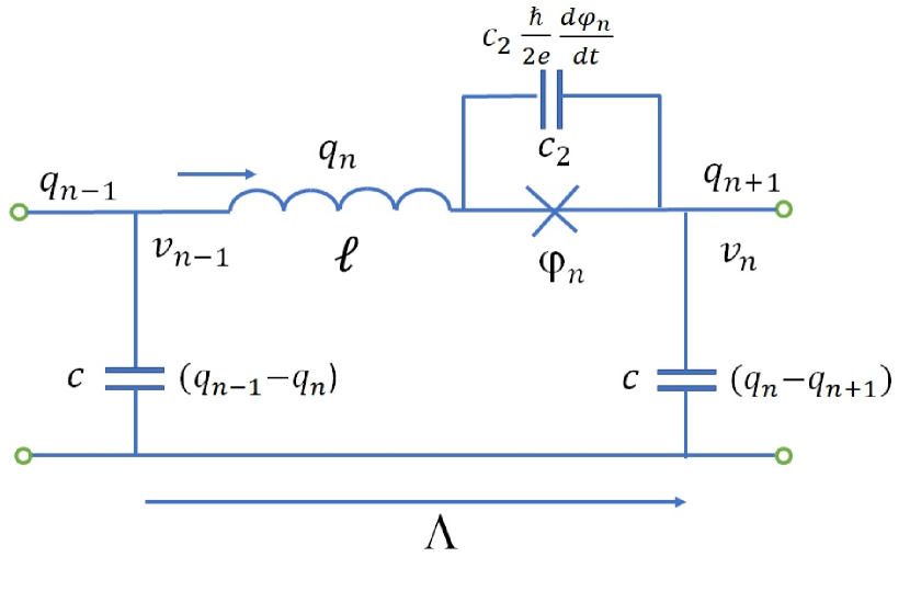
Figure 1: Dissipationless JTL.

Assuming smooth variance of $\varphi_{n}$ and $q_{n}$ with $n$, we can write down (1) in the continuum approximation as

$$\frac{1}{C}\frac{\partial^{2}q}{\partial x^{2}} =L\frac{\partial^{2}q}{\partial t^{2}}+E_{J}\frac{\partial\varphi}{\partial t}\,,$$ (2a)

$$\frac{\partial q}{\partial t} =I_{c}\sin\varphi+C_{2}E_{J}\frac{\partial^{2}\varphi}{\partial t^{2}}\,,$$ (2b)

where $\Lambda$ is the period of the line, $C=c/\Lambda$, $C_{2}=c_{2}\Lambda$, $L=\ell/\Lambda$, and $E_{J}=\hbar/(2e\Lambda)$. In Appendix A we rederive Eqs. (1) and (2) in the framework of Lagrange and Hamilton approaches. Another form of (2a) can be obtained after we introduce the voltage between the wires $v$:

$$\frac{\partial v}{\partial x} =-L\frac{\partial^{2}q}{\partial t^{2}}-E_{J}\frac{\partial\varphi}{\partial t}\,,$$ (3a)

$$v =-\frac{1}{C}\frac{\partial q}{\partial x}\,.$$ (3b)

II.2 Waves and shock waves

For $C_{2}=0$ equations (3) and (2b) take the form

$$\frac{\partial v}{\partial x} =-L\frac{\partial}{\partial t}\left(I+I_{L}\varphi\right)\,,$$ (4a)

$$C\frac{\partial v}{\partial t} =-\frac{\partial I}{\partial x}\,,$$ (4b)

where $I_{L}=E_{J}/L$. In (4a) and (4b) (and everywhere else in this paper) $I\equiv I_{c}\sin\varphi$. If all variables in (4a) and (4b) are differentiable functions of $x$ and $t$, these equations can be combined in a single wave equation for $I$

$$\frac{\partial^{2}I}{\partial x^{2}}-\frac{\partial}{\partial t}\left[\frac{1}{u^{2}(I)}\frac{\partial I}{\partial t}\right]=0\,,$$ (5)

where

$$\frac{1}{u^{2}(I)}=CL_{eff}(I)\,,$$ (6)

and the effective inductance $L_{eff}(I)$ is

$$L_{eff}=L\left(1+\frac{I_{L}}{I_{c}\cos\varphi}\right)=L\left(1+\frac{I_{L}}{(I_{c}^{2}-I^{2})^{1/2}}\right)\;.$$ (7)

Note that $u(I)$ is the velocity propagation of small amplitude disturbances on a homogeneous background, and that this velocity is given by (6) even for nonzero $C_{2}$, when the frequency of the disturbances $\omega\to 0$.

In addition, (4) admits moving discontinuities in the form

$$I(x,t) =I_{1}(x,t)H(-S(x,t))+I_{2}(x,t)H(S(x,t))\,,$$ (8a)

$$v(x,t) =v_{1}(x,t)H(-S(x,t))+v_{2}(x,t)H(S(x,t))\,,$$ (8b)

where $H(x)$ is the Heaviside step function and $I_{1},I_{2}$ ($v_{1},v_{2}$) are functions with continuous derivatives. On substitution (8) into (4) we obtain (keeping only the singular terms)

$$\left[\frac{\partial S}{\partial x}\Delta v+\frac{\partial S}{\partial t}L\left(\Delta I+I_{L}\Delta\varphi\right)\right]\delta(S(x,t)) =0\;,$$ (9a)

$$\left(C\frac{\partial S}{\partial t}\Delta v+\frac{\partial S}{\partial x}\Delta I\right)\delta(S(x,t)) =0$$ (9b)

(everywhere in this paper $\Delta F\equiv F_{2}-F_{1}$, for any function $F$). The velocity of the discontinuity propagation is

$$U=-\left.\frac{\partial S/\partial t}{\partial S/\partial x}\right|_{S=0}\,$$ (10)

(in the simplest case $S(x,t)=t-x/U$). Equation (9) therefore becomes

$$\Delta v-UL\left(\Delta I+I_{L}\Delta\varphi\right) =0\ ,$$ (11a)

$$UC\Delta v-\Delta I =0\ .$$ (11b)

Eliminating $\Delta v$ we find

$$\frac{1}{\overline{U}^{2}(I_{1},I_{2})}=1+I_{L}\frac{\Delta\varphi}{\Delta I}=1+\frac{I_{L}\Delta\varphi}{I_{c}\Delta\sin\varphi}\,,$$ (12)

where $\overline{U}=U/u_{T}$, and $u_{T}^{2}=1/LC$. The difference between $\overline{U}$ and $\overline{u}=u(I)/u_{T}$ is illustrated on Fig. 2.

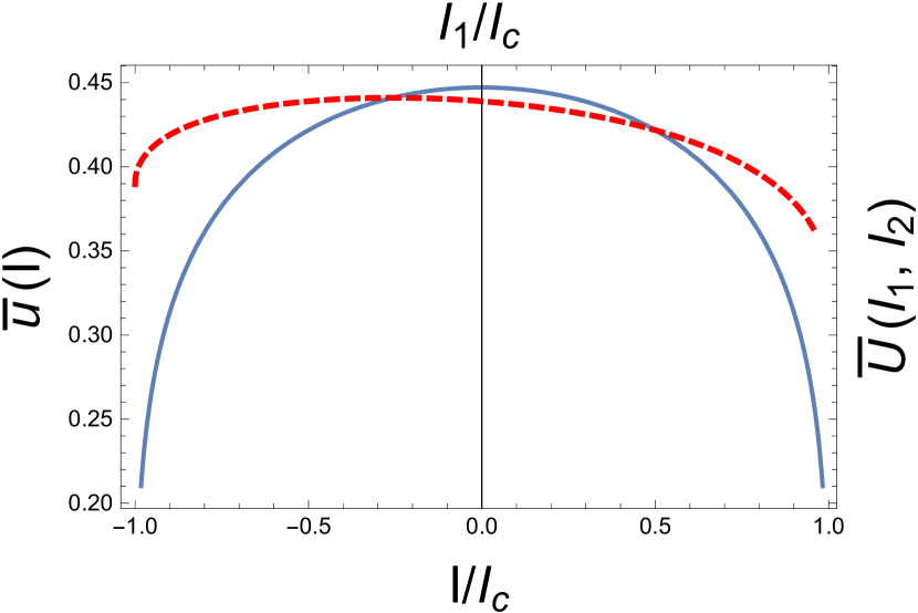
Figure 2: Small amplitude disturbance propagation velocity $\overline{u}(I)$ according to (6) (blue solid line) and shock propagation velocity $\overline{U}(I_{1},I_{2})$ according to (12) (red dashed line) for $I_{L}=4I_{c}$ and $I_{2}=.5I_{c}$.

In the particular case $L=0$, (12) should be presented as

$$\frac{1}{U^{2}}=\frac{E_{J}C\Delta\varphi}{I_{c}\Delta\sin\varphi}\,.$$ (13)

In the symmetric case

$$I_{2}=I_{0}=I_{c}\sin\frac{\Delta\varphi}{2},\hskip 14.22636ptI_{1}=-I_{0}=-I_{c}\sin\frac{\Delta\varphi}{2}\,,$$ (14)

(13) takes the form

$$\frac{1}{U^{2}}=\frac{E_{J}C}{I_{0}}\sin^{-1}\left(\frac{I_{0}}{I_{c}}\right)\,.$$ (15)

Expanding $\sin^{-1}$ in power series we obtain

$$\frac{1}{U^{2}}=\frac{E_{J}C}{I_{c}}\left(1+\frac{I_{0}^{2}}{6I_{C}^{2}}+\dots\right)\,.$$ (16)

The velocity, calculated in Ref. katayama up to the second order in $I_{0}/I_{c}$, coincides with that given by (16) (also truncated to same order).

II.2.1 Shock wave in the discrete JTL

Actually, discontinuous solutions (8) mean that the continuum approximation is no longer adequate, and discrete model of the JTL, which resolves the discontinuity, should be considered. Let us start from rederiving (12) in the framework of the discrete model.

Assuming $c_{2}=0$, we can rewrite (1a) as

$$\frac{1}{c}\left(q_{n+1}-2q_{n}+q_{n-1}\right)=\frac{d}{dt}\left(\ell I_{c}\sin\varphi_{n}+\frac{\hbar}{2e}\varphi_{n}\right)\,.$$ (17)

Now let us sum up (17) between the two points, one just ahead of the steep portion of the wave front, and the other - just behind it. The r.h.s. of the equation has a time derivative only because of the motion of the steep portion, and the slower changes due to the motion of the parts of the wave with moderate slope can be neglected. Hence after the summation we obtain

$$\frac{\Lambda I_{c}}{cU}\Delta\sin\varphi=\frac{U}{\Lambda}\left(\ell I_{c}\Delta\sin\varphi+\frac{\hbar}{2e}\Delta\varphi\right)\,,$$ (18)

which is just (12). (While calculating the l.h.s. of (18) we took into account (1b).)

Let us continue studying (17). Introducing the new variable $i_{n}=dq_{n}/dt$ and considering small amplitude disturbance of a uniform state

$$i_{n}=I_{2}-\Delta I\cdot x_{n}\;,$$ (19)

we can linearise the problem with respect to $\Delta I$. Introducing dimensionless time $\tau=2t/\sqrt{c\ell_{eff}}$, where

$$\ell_{eff}=\ell+\frac{\hbar/2e}{\sqrt{I_{c}^{2}-I_{2}^{2}}}\;,$$ (20)

we obtain from (17)

$$\frac{d^{2}x_{n}}{d\tau^{2}}=\frac{1}{4}(x_{n+1}-2x_{n}+x_{n-1})\,.$$ (21)

We will consider a signalling problem for a semi-infinite line $n\geq 0$. The problem is characterised by the boundary condition $x_{0}(\tau)=1$ and the initial conditions $x_{n}(0)=\dot{x}_{n}(0)=0$ for $n\geq 1$.

To solve (21) we will use the Laplace transform, in the beginning following Ref. bulla . For a given time-dependent function $f(\tau)$, we define the Laplace transform $F(s)={\cal L}\{f(\tau)\}$ as

$$F(s)=\int_{0}^{\infty}{\rm d}\tau\,e^{-s\tau}f(\tau)\ .$$ (22)

Laplace transforming (21) and using the corollary of (22)

$$f^{\prime}(\tau)\Longleftrightarrow sF(s)-f(0)\ ,$$ (23)

we obtain the difference equation for $X_{n}(s)={\cal L}\{x_{n}(t)\}$

$$X_{n+1}-2(1+2s^{2})X_{n}+X_{n-1}=0\ ,$$ (24)

with the boundary conditions $X_{0}(s)=1/s$, $\lim_{n\to\infty}X_{n}(s)=0$. Solving (24):

$$X_{n}(s)=\frac{1}{s}\left[1-2s\left(\sqrt{s^{2}+1}-s\right)\right]^{n}\;,$$ (25)

and taking into account the known result abram

$$(\sqrt{s^{2}+1}-s)^{k}\Longleftrightarrow\frac{k}{\tau}J_{k}(\tau)\;,$$ (26)

where $J_{k}$ is the Bessel function, we obtain

$$x_{n}(\tau)=1+\sum_{k=1}^{n}C^{n}_{k}(-1)^{k}2^{k}k\frac{d^{k-1}}{d\tau^{k-1}}\left(\frac{J_{k}(\tau)}{\tau}\right).$$ (27)

Using the recurrence relation

$$2\frac{d}{d\tau}J_{k}(\tau)=J_{k-1}(\tau)-J_{k+1}(\tau)\;,$$ (28)

we can present any $x_{n}$ as a linear combination of Bessel functions. A snapshot of the shock wave given by (27) is presented on Fig. 3.

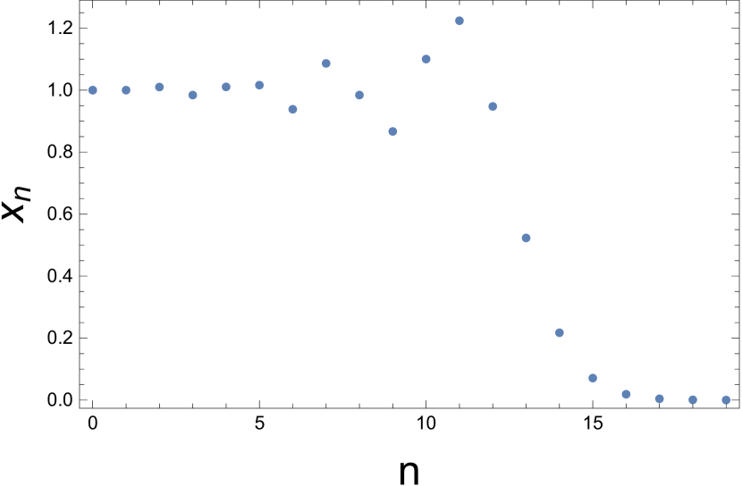
Figure 3: A snapshot of the shock wave given by (27) ($\tau=25$).

The input voltage is

$$v_{0}(t) = \frac{1}{c}\left[q_{0}(t)-q_{1}(t)\right]=\frac{\Delta I}{c}\int_{0}^{t}dt[x_{1}(t)-1]$$ (29)

$$= \sqrt{\frac{\ell_{eff}}{c}}\Delta I\int_{0}^{\tau}d\tau\frac{J_{1}(\tau)}{\tau}\ .$$

In particular, using known formula for the integral from Bessel function prudnikov , we obtain an expected result

$$v_{0}(\infty)=\sqrt{\frac{\ell_{eff}}{c}}\Delta I=\sqrt{\frac{L_{eff}}{C}}\Delta I=Z_{eff}\Delta I\;.$$ (30)

These results show how the (quasi) discontinuous shock wave can be generated. If there is a semi-infinite JTL with the constant current source at the end (and in a stationary state, with the input voltage being equal to zero), and then suddenly the current of the source changes to another constant value, the shock wave will start to propagate.

In order to compute the inverse Laplace transform one can either use correspondence tables, like we did above, or compute the Bromwich integral. More specifically, there exists the following theorem.

If the function $F(s)$ is analytic in the half plane Re $s>s_{0}$, goes to zero when $|s|\to\infty$ in any half plane Re $s\geq a>s_{0}$ uniformly with respect to arg $s$ and the integral

$$\int_{a-i\infty}^{a+i\infty}F(s)ds$$

absolutely converges, then $F(s)$ is the Laplace image of the function

$$f(\tau)=\frac{1}{2\pi i}\int_{a-i\infty}^{a+i\infty}ds\,e^{s\tau}F(s)$$ (31)

(the integration is done along the vertical line Re$(s)=a$ in the complex plane).

From (27) follows

$$\frac{dx_{n}}{d\tau}=\sum_{k=1}^{n}C^{n}_{k}(-1)^{k}2^{k}k\frac{d^{k}}{d\tau^{k}}\left(\frac{J_{k}(\tau)}{\tau}\right)\,.$$ (32)

We will try to get more explicit analytic result for the quantity using Bromwich integral. From (25) we obtain

$$\frac{dx_{n}}{d\tau}=\frac{1}{2\pi i}\int_{a-i\infty}^{a+i\infty}ds$$

$$\exp\left\{s\tau+n\ln\left[1-2s\left(\sqrt{s^{2}+1}-s\right)\right]\right\}\;.$$ (33)

Expanding the logarithm in (II.2.1) with respect to $s$ and keeping only the lowest order terms we get

$$\frac{dx_{n}}{d\tau}=\frac{1}{2\pi i}\int_{a-i\infty}^{a+i\infty}ds\exp\left[s(\tau-2n)+\frac{n}{3}s^{3}\right]\;.$$ (34)

The contour of integration in (34) can be deformed so that it will start at the point at infinity with argument $-\pi/3$ and will end at the point at infinity with argument $\pi/3$. Hence the integral determines the Airy function abram

$$\frac{dx_{n}}{d\tau}=n^{-1/3}\text{Ai}\left[n^{-1/3}(2n-\tau)\right]\;.$$ (35)

Equation (35) describes the shock front at $n\sim\tau/2$, exponential decrease of the signal with increasing $n$ for $n>\tau/2$, and oscillations and power law decrease of the signal with decreasing $n$ for $n<\tau/2$. Equations (32) and (35) are plotted on Fig. 4. Comparison of the graphs shows that the approximate formula (35) correctly describes front of the shock wave, but not its wake.

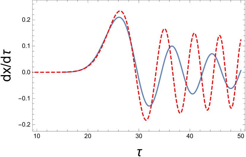
Figure 4: Equation (32) (solid blue line) and (35) (dashed red line) for $n=12$.

In the linear approximation to (17), as we see from (35), the shock wave spreads indefinitely (because of the dispersion present in the system). An attempt to understand whether the nonlinear terms in the equation will stop the spreading, is presented in Appendix B.

III Shock waves in the JTL with ohmic dissipation

Let us add to the JTL ohmic resistors, thus considering transmission line presented on Fig. 5. In this case (2b) changes to

$$\frac{\partial q}{\partial t}=I_{c}\sin\varphi+\frac{E_{J}}{R_{2}}\frac{\partial\varphi}{\partial t}+C_{2}E_{J}\frac{\partial^{2}\varphi}{\partial t^{2}}\,,$$ (36)

and (3b) changes to

$$v=-\frac{1}{C}\frac{\partial q}{\partial x}-R\frac{\partial^{2}q}{\partial t\partial x}\,.$$ (37)

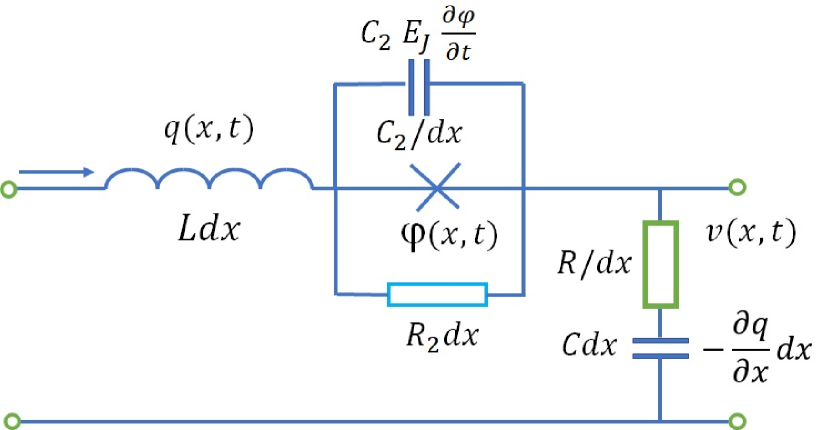
Figure 5: JTL with ohmic resistors shunting the JJ and in series with the ground capacitor.

III.1 The travelling waves

The system of equations (3a), (36), (37) has a set of particularly simple solutions, called traveling waves, when dependence of all the quantities upon $x,t$ is the dependence upon a single parameter $t-x/U$ (for the sake of definiteness, we consider right going waves). These solutions satisfy ordinary differential equation, which can be obtained after eliminating $v$ and $q$:

$$RCC_{2}L\frac{d^{3}\varphi}{dt^{3}}+\left[\frac{RC}{R_{2}}+C_{2}\left(1-\overline{U}^{2}\right)\right]L\frac{d^{2}\varphi}{dt^{2}}$$

$$+\left[\frac{L}{R_{2}}\left(1-\overline{U}^{2}\right)+\frac{RCI_{c}}{I_{L}}\cos\varphi\right]\frac{d\varphi}{dt}$$

$$+\frac{I_{c}}{I_{L}}\sin\varphi\left(1-\overline{U}^{2}\right)-\overline{U}^{2}\varphi+A=0\,,$$ (38)

where $A$ is an arbitrary constant (we integrated once).

We are looking for a solution which tends to constants at infinity

$$\lim_{t\to-\infty}I=I_{2},\;\;\lim_{t\to+\infty}I=I_{1}\,.$$ (39)

For given $I_{1}$ and $I_{2}$, the parameters $U,A$ must satisfy

$$I_{i}-\overline{U}^{2}\left(I_{i}+I_{L}\varphi_{i}\right)+A=0\,,\;\;\;i=1,2\,.$$ (40)

Eliminating $A$ we recover (12). We see that the relation between the shock velocity and the values of current on both sides of the shock is dissipation independent.

Equation (III.1) with the boundary conditions (39) can be presented as

$$RCC_{2}L\frac{d^{3}\varphi}{dt^{3}}+\left[\frac{RCL}{R_{2}}+C_{2}L\left(1-\overline{U}^{2}\right)\right]\frac{d^{2}\varphi}{dt^{2}}$$

$$+\left[\frac{L}{R_{2}}\left(1-\overline{U}^{2}\right)+\frac{RCI_{c}}{I_{L}}\cos\varphi\right]\frac{d\varphi}{dt}=M(\varphi)\,,$$ (41)

where

$$M(\varphi) = \left[\varphi\cdot\Delta\sin\varphi-\sin\varphi\cdot\Delta\varphi+\varphi_{2}\sin\varphi_{1}-\varphi_{1}\sin\varphi_{2}\right]$$ (42)

$$\cdot \frac{I_{c}}{I_{c}\Delta\sin\varphi+I_{L}\Delta\varphi}\,.$$

Note that $M(\varphi_{1})=M(\varphi_{2})=0$, and that for weak shock ($|I_{2}-I_{1}|\ll|I_{2}|$), $M(\varphi)$ is simplified to

$$M(\varphi)=\overline{u}_{0}^{2}\frac{\tan\varphi_{0}}{2}(\varphi-\varphi_{1})(\varphi-\varphi_{2})\,.$$ (43)

Equation (III.1) is very close to that describing dc driven resistively shunted self-resonant Josephson tunnel junction imry ; kruger ; likharev .

III.2 Newtonian analogy

III.2.1 Stability of the equilibrium points

If $\sqrt[3]{RCC_{2}L}$ is much less than all the other time scales in the problem, the term with the third derivative in (III.1) can be discarded, and the latter takes the form

$$\frac{d^{2}\varphi}{d\tau^{2}}+(\gamma_{2}+\gamma_{1}\cos\varphi)\frac{d\varphi}{d\tau}+\frac{d\Pi(\varphi)}{d\varphi}=0\,,$$ (44)

where

$$\tau=\frac{t}{T},\;\;\;\gamma_{2} = \frac{L}{R_{2}T}\left(1-\overline{U}^{2}\right),\;\;\;\gamma_{1}=\frac{RCI_{c}}{I_{L}T},$$

$$T^{2} = \frac{RCL}{R_{2}}+C_{2}L\left(1-\overline{U}^{2}\right)\,,$$ (45)

and

$$\Pi(\varphi) = \Big{[}-\frac{\varphi^{2}}{2}\cdot\Delta\sin\varphi+(1-\cos\varphi)\cdot\Delta\varphi$$

$$- \varphi\cdot(\varphi_{2}\sin\varphi_{1}-\varphi_{1}\sin\varphi_{2})\Big{]}\cdot\frac{I_{c}}{I_{c}\Delta\sin\varphi+I_{L}\Delta\varphi}\,.$$

Equation (44) describes motion of a Newtonian particle in the potential well $\Pi(\varphi)$, shown on Fig. 6, and in the presence of friction force (the term proportional to $d\varphi/d\tau$).

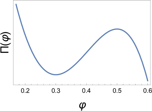
Figure 6: Potential energy of the fictitious particle (arbitrary units); $\varphi_{1}=.3,\varphi_{2}=.5$.

The particle (asymptotically) starts in the upper equilibrium position and finishes in the lower equilibrium position.

The values $\varphi_{1}$ and $\varphi_{2}$ enter into (12) in a symmetrical way. However, due to ohmic resistance, inevitably present in the system, only one direction of shock propagation is possible. The potential energy of the fictitious particle corresponding to the state before the shock should be higher than that behind the shock. This condition can be enhanced even further. The potential energy shouldn’t have any local extrema between $\varphi_{1}$ and $\varphi_{2}$ (local extremum means splitting of a single shock into two.) Thus the potential energy should have at $\varphi_{2}$ local maximum, and at $\varphi_{1}$ - local minimum. This is equivalent to inequalities

$$u(I_{1})>U(I_{1},I_{2})>u(I_{2})\,,$$ (47)

which reflect the well known fact: the shock velocity is lower than the sound velocity in the region behind the shock, but higher than the sound velocity in the region before the shock whitham . Actually, the stability analysis of the equilibrium points can be performed for (III.1) with the same result.

Because $\sin\varphi$ is concave downward for $0<\varphi<\pi/2$, and concave upward for $-\pi/2<\varphi<0$, $M(\varphi)$ can not have zeros between $\varphi_{1}$ and $\varphi_{2}$ having the same sign, thus there can exist shock between any pair of currents of the same sign. On the other hand, the inequalities (47) pose limitations on the values of positive and negative currents, between which a single shock can exist. So returning to Fig. 2 we understand, that the red dashed curve inside the dome describes shocks, for which $I_{2}$ is the current before the shock. The red dashed curve to the right of the dome and the red dashed curve to the left of the dome which lies below $\overline{u}(I_{2})$ describe the shocks, for which $I_{2}$ is the current after the shock.

III.2.2 The shock profile

Though (44) is non integrable analytically in the general case, qualitatively the nature of the motion from one equilibrium position to the other is clear (at least for $\gamma\gg 1$ and $\gamma\ll 1$). In the former regime the particle moves monotonically from one equilibrium position to the other, in the latter - the particle oscillates in the potential well, and weak friction leads to slow decrease of the oscillations amplitude with time.

If $C_{2}=0$ and $\sqrt{L/(RR_{2}C)}\ll 1$, the terms with $\gamma_{2}$ and the second derivative in the l.h.s. of (44) can be discarded. If $C_{2}=0$ and $\sqrt{L/(RR_{2}C)}\gg 1$, the terms with $\gamma_{1}$ and the second derivative can be discarded. The resulting equations describe motion of the strongly overdamped particle and can be easily integrated analytically. We obtain

$$t =\frac{RCI_{c}}{I_{L}}\int\frac{\cos\varphi d\varphi}{M(\varphi)},\hskip 31.2982pt\sqrt{\frac{L}{RR_{2}C}}\ll 1\,,$$ (48a)

$$t =\frac{L}{R_{2}}\left(1-\overline{U}^{2}\right)\int\frac{d\varphi}{M(\varphi)},\hskip 14.22636pt\sqrt{\frac{L}{RR_{2}C}}\gg 1\,.$$ (48b)

In both cases the shape of the shock depends only upon $\varphi_{1}$ and $\varphi_{2}$ and is independent upon the parameters of the transition line. Equation (48a) is presented graphically on Fig. 7.

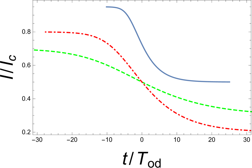
Figure 7: Shock profile according to (48a) for $I_{L}=.5I_{c}$. Blue solid line corresponds to $I_{1}=.5I_{c}$, $I_{2}=.95I_{c}$, red dot-dashed line - to $I_{1}=.2I_{c}$, $I_{2}=.8I_{c}$, green dashed line - to $I_{1}=.3I_{c}$, $I_{2}=.3I_{c}$, $T_{od}=RCI_{c}/I_{L}$.

For weak shock in both cases we obtain

$$I=I_{0}-\frac{\Delta I}{2}\tanh(\alpha t)\,,$$ (49)

where $I_{0}=(I_{1}+I_{1})/2$, and

$$\alpha =\frac{\Delta u}{2u_{0}}\frac{1}{RC},\hskip 85.35826pt\sqrt{\frac{L}{RR_{2}C}}\ll 1$$ (50a)

$$\alpha =\frac{I_{L}}{I_{c}\cos\varphi_{0}}\frac{\Delta u}{2u_{0}}\frac{R_{2}}{L\left(1-\overline{U}^{2}\right)},\hskip 14.22636pt\sqrt{\frac{L}{RR_{2}C}}\gg 1\,.$$ (50b)

Consider now the case of $R=0$, $C_{2}\gg L/R_{2}^{2}$ (which corresponds to $\gamma_{2}\ll 1$). The results of integration of (44) in this case are presented on Figs. 8 and 9. The phase (current) in the shock wave oscillates, in strong contrast to monotonous change in the case of zero shunting capacitance, presented on Fig. 7.

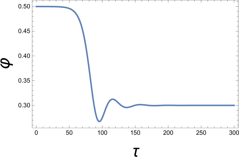
Figure 8: Shock profile according to (44); $I_{L}=.5I_{c},\varphi_{1}=.3,\varphi_{2}=.5,\gamma_{2}=.1$, $\gamma_{1}=0$.

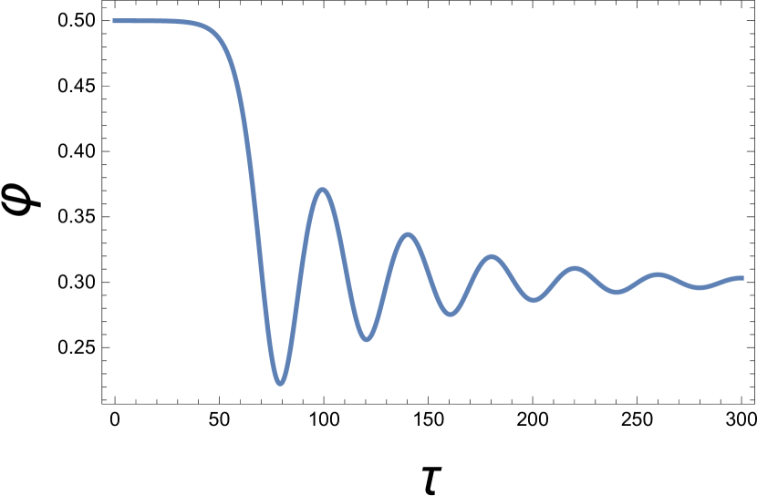
Figure 9: Shock profile according to (44); $I_{L}=.5I_{c},\varphi_{1}=.3,\varphi_{2}=.5,\gamma_{2}=.03$, $\gamma_{1}=0$.

III.3 Weak damping: the method of time averaging

When the term with the third derivative in (III.1) is kept, the latter can be written as

$$\beta\frac{d^{3}\varphi}{d\tau^{3}}+\frac{d^{2}\varphi}{d\tau^{2}}+\gamma(\varphi)\frac{d\varphi}{d\tau}+\frac{d\Pi(\varphi)}{d\varphi}=0\,,$$ (51)

where $\beta=RCC_{2}L/T^{3}$. Equation (51) describes jerky linz ; sprott particle. Analysis of the local stability of the fixed point $\varphi=\varphi_{1}$ is exactly the same as it was in Section III.2. Global stability of the point is less obvious. In any case, in this Section we will consider the regime $C_{2}\gg L/R_{2}^{2},R^{2}C^{2}/L$ (which corresponds to $\beta,\gamma\ll 1$), where the situation with the global stability is clear (see (III.3) and the sentence immediately after it).

We will use the method of time averaging, which we formulate below. We assume that we know the undamped solution $\varphi_{ud}(\tau;{\cal E})$, satisfying equation

$$\frac{1}{2}\left(\frac{d\varphi_{ud}}{d\tau}\right)^{2}+\Pi(\varphi_{ud})={\cal E}\,,$$ (52)

and express damped oscillations as

$$\varphi(\tau)=\varphi_{ud}(\tau;{\cal E}(\tau))\,.$$ (53)

To find ${\cal E}(\tau)$, notice that from (44) follows

$$\frac{d}{d\tau}\left[\frac{1}{2}\left(\frac{d\varphi}{d\tau}\right)^{2}+\Pi(\varphi)\right]=-\gamma(\varphi)\left(\frac{d\varphi}{d\tau}\right)^{2}-\beta\frac{d\varphi}{d\tau}\frac{d^{3}\varphi}{d\tau^{3}}\,.$$

Ignoring terms of the order of $\beta\gamma$ and $\beta^{2}$, (III.3) can be written as

$$\frac{d}{d\tau}\left[\frac{1}{2}\left(\frac{d\varphi}{d\tau}\right)^{2}+\Pi(\varphi)\right]=-\Gamma(\varphi)\left(\frac{d\varphi}{d\tau}\right)^{2}\,,$$

where $\Gamma(\varphi)=\gamma(\varphi)+\beta dM(\varphi)/d\varphi$. Note, that $\Gamma(\varphi)$ is positive for any $\varphi$. For example, when $R=\infty$,

$$\Gamma(\varphi)=\frac{RCC_{2}LI_{c}}{T^{3}I_{L}}\left(1-\overline{U}^{2}\right)\frac{(I_{c}\cos\varphi+I_{L})\Delta\sin\varphi}{I_{c}\Delta\sin\varphi+I_{L}\Delta\varphi}\,.$$ (56)

We’ll assume that ${\cal E}(\tau)$ satisfies equation

$$\frac{d{\cal E}}{d\tau}=-\left<\Gamma(\varphi)\left(\frac{d\varphi}{d\tau}\right)^{2}\right>_{ud}\equiv-{\cal A}({\cal E})\,,$$ (57)

where the averaging is with respect to the period of the undamped oscillation with the energy ${\cal E}$. The averaging in (57) is performed as

$$\frac{1}{T}\int_{0}^{T}\Gamma(\varphi)\left(\frac{d\varphi_{ud}}{dt}\right)^{2}dt=\frac{2\int d\varphi\Gamma(\varphi)\sqrt{{\cal E}-\Pi(\varphi)}}{\int d\varphi/\sqrt{{\cal E}-\Pi(\varphi)}}\,,$$ (58)

the limits of integration in both integrals being found from the equation ${\cal E}-\Pi(\varphi)=0$. Integrals defining ${\cal A}({\cal E})$ being calculated, the solution of (57)

$$\tau=-\int\frac{d{\cal E}}{{\cal A}({\cal E})}\,,$$ (59)

together with (53), gives parametric representation of the particle motion. In Appendix C we’ll see how all this works for weak shocks.

III.4 The JTL with ohmic resistor in series with the JJ

Let us now introduce ohmic resistor in a way different from that considered previously, constructing the transmission line presented on Fig. 10.

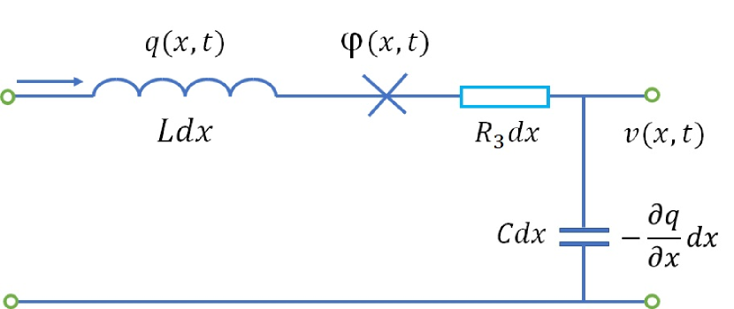
Figure 10: JTL with ohmic resistor in series with the JJ.

In this case (4) changes to

$$\frac{\partial v}{\partial x} =-L\frac{\partial}{\partial t}\left(I+I_{L}\varphi\right)-R_{3}I\,,$$ (60a)

$$C\frac{\partial v}{\partial t} =-\frac{\partial I}{\partial x}$$ (60b)

The analysis of moving discontinuities presented in Section II.2 can be repeated verbatim, hence (i) the discontinuous solutions are allowed for (60), (ii) the velocity of their propagation is given by (12). Ohmic resistors in the present case neither lead to finite width of shocks, nor influence the velocity of their propagation. Notice, that in the presence of the higher order derivatives in the JTL equations, which is the case when ohmic dissipation is taken into account, the terms with $\delta^{\prime}(x-Ut)$ will appear if we substitute discontinuous functions of coordinates, and there are no other that singular term to balance it.

IV The simple wave approximation

IV.1 The dissipationless JTL

Let us start from the dissipationless transmission line, described by (5). The simple wave approximation rabinovich ; vinogradova for the equation may be obtained by changing by brute force (5) into two decoupled equations for right and left going waves

$$\frac{\partial I}{\partial x}\pm\frac{1}{u(I)}\frac{\partial I}{\partial t}=0\,.$$ (61)

Equation (61), in distinction to (5), can be easily solved analytically whitham ; billingham .

Consider the signalling problem for $x\geq 0$, characterised by the initial and boundary conditions

$$I(x,0) =I_{2}\,,$$ (62a)

$$I(0,t) =I_{1}\,.$$ (62b)

The solution of (61) containing the shock is

$$I(x,t)=\left\{\begin{array}[]{ll}I_{2},&\text{for}\;\;\;x>U(I_{1},I_{2})t,\\ I_{1},&\text{for}\;\;\;0<x<U(I_{1},I_{2})t.\end{array}\right.$$ (65)

However, the shock can exist only provided $|I_{1}|<|I_{2}|$. For $|I_{1}|>|I_{2}|$ the solution of (61) contains an expansion fan whitham ; billingham

$$I(x,t)=\left\{\begin{array}[]{ll}I_{2},&\text{for}\;\;\;x>u(I_{2})t,\\ {\cal I}(x/u_{T}t),&\text{for}\;\;\;u(I_{1})t\leq x\leq u(I_{2})t,\\ I_{1},&\text{for}\;\;\;0<x<u(I_{1})t,\end{array}\right.$$ (69)

where the function ${\cal I}$ is obtained by inverting (6)

$${\cal I}(\overline{u})=\left[I_{c}^{2}-\frac{I_{L}^{2}\overline{u}^{4}}{(1-\overline{u}^{2})^{2}}\right]^{1/2}\,.$$ (70)

IV.2 Shock formation in the JTL with ohmic dissipation

When ohmic resistor in series with the ground capacitor is additionally taken into account, (5) is modified to

$$\frac{\partial^{2}}{\partial x^{2}}\left(I+RC\frac{\partial I}{\partial t}\right)=\frac{\partial}{\partial t}\left[\frac{1}{u^{2}(I)}\frac{\partial I}{\partial t}\right]\,.$$ (71)

Following the example of Section IV.1, we attempt to take the "square root" of the operator, acting upon $I$ in the l.h.s. of (71), and postulate that right and left going waves satisfy decoupled equations

$$\frac{\partial I}{\partial t}\pm u(I)\frac{\partial}{\partial x}\left(I+\nu\frac{\partial I}{\partial t}\right)=0\,,$$ (72)

where $\nu=RC/2$. Equations (72) are the generalization of the simple wave approximation to the case of JTL with ohmic dissipation.

For the traveling right going wave, from (72) we obtain

$$\frac{1}{U}\frac{d}{dt}\left(I+\nu\frac{dI}{dt}\right)-\frac{1}{u(I)}\frac{dI}{dt}=0\,.$$ (73)

Integrating with respect to $t$ from $-\infty$ to $+\infty$ and taking into account the boundary conditions (39), we obtain

$$\frac{1}{U}=\frac{1}{\Delta I}\int_{I_{1}}^{I_{2}}\frac{dI}{u(I)}\,.$$ (74)

More explicitly, (74) is

$$\frac{1}{\overline{U}(I_{1},I_{2})}=\frac{1}{\Delta I}\int_{I_{1}}^{I_{2}}dI\left[1+\frac{I_{L}}{(I_{c}^{2}-I^{2})^{1/2}}\right]^{1/2}\,.$$ (75)

Equation (75) is slightly different from the exact (12), but the results are very close. We didn’t plot the curve given by (75) on Fig. 2, because it would absolutely merge with the curve given by (12). Another argument, which convinces us in validity of (72), is the fact that the weak shock profile (49), with $\alpha$ given by (50a), is a solution of (72).

Equation (72) hopefully is able to describe the shock formation for the signalling problem. To make this task easier, we propose to additionally simplify (72) to

$$\frac{\partial u}{\partial t}\pm u\frac{\partial}{\partial x}\left(u+\nu\frac{\partial u}{\partial t}\right)=0\,.$$ (76)

Equation (76) may be called the modified Burgers equation (mBE). In Appendix D we study the symmetry of the equation.

Now let us consider the JTL with ohmic resistor in series with the JJ. From (60) follows

$$\frac{\partial^{2}I}{\partial x^{2}}-\frac{\partial}{\partial t}\left[\frac{1}{u^{2}(I)}\frac{\partial I}{\partial t}+R_{3}CI\right]=0.$$ (77)

The generalization of the simple wave approximation to this case is

$$\frac{\partial I}{\partial t}+\mu u^{2}(I)I\pm u(I)\frac{\partial I}{\partial x}=0\,,$$ (78)

where $\mu=R_{3}C/2$. Discontinuities formation for the solutions of (78) is studied in Appendix E.

V Discussion

We hope that the results obtained in the paper are applicable to kinetic inductance based traveling wave parametric amplifiers based on a coplanar waveguide architecture. Onset of shock-waves in such amplifiers is an undesirable phenomenon. Therefore, shock waves in various JTL should be further studied, which was one of motivations of the present work.

Recently, quantum mechanical description of JTL in general and parametric amplification in such lines in particular started to be developed, based on quantisation techniques in terms of discrete mode operators reep , continuous mode operators fasolo , a Hamiltonian approach in the Heisenberg and interaction pictures greco , or the quantum Langevin method yuan It would be interesting to understand in what way the results of the present paper are changed by quantum mechanics. Particularly interesting looks studying of quantum ripples over a semi-classical shock glazman and fate of quantum shock waves at late times glazman2 .

VI Conclusions

We have analytically calculated the velocity of propagation and structure of shock waves in the transmission line constructed from the JJ, linear inductors, capacitors and ohmic resistors. In the absence of ohmic dissipation the shocks are sharp. As such they remain when ohmic resistors are introduced in series with the JJ and linear inductors. When ohmic resistors shunt the JJ or are in series with the ground capacitors, the shocks are broadened. The shock width is inversely proportional to the resistance shunting JJ, or proportional to the resistance in series with the ground capacitor. In all the cases considered, ohmic resistors (and shunting capacitors) don’t influence the shock propagation velocity. We formulate the simple wave approximation for the JTL with ohmic dissipation and study an alternative to the shock wave - an expansion fan - in the framework of this approximation.

Data Availability Statement

The data that support the findings of this study are available from the corresponding author upon reasonable request.

Appendix A The Lagrangian and the Hamiltonian of the JTL

Let us rederive (1) in the framework of Lagrange approach. The Lagrangian ${\cal L}$ is

$${\cal L}=\frac{\ell}{2}\sum_{n}\left(\frac{dq_{n}}{dt}\right)^{2}+\frac{c_{2}\hbar^{2}}{8e^{2}}\sum_{n}\left(\frac{d\varphi_{n}}{dt}\right)^{2}$$ (79)

$$-\frac{1}{2c}\sum_{n}\left(q_{n}-q_{n+1}\right)^{2}+\frac{\hbar}{2e}I_{c}\sum_{n}\cos\varphi_{n}+\frac{\hbar}{2e}\sum_{n}\frac{dq_{n}}{dt}\varphi_{n}\,.$$

Lagrange equations have the form

$$\frac{d}{dt}\left(\frac{\partial{\cal L}}{\partial\dot{Q}}\right)-\frac{\partial{\cal L}}{\partial Q}=0,$$ (80)

where $Q$ is any of the dynamical variables. Lagrange equation corresponding to $q_{n}$

$$\ell\frac{d^{2}q_{n}}{dt^{2}}+\frac{\hbar}{2e}\frac{d}{dt}\varphi_{n}+\frac{1}{c}\left(2q_{n}-q_{n+1}-q_{n-1}\right)=0\,,$$ (81)

reproduces (1a). Lagrange equation corresponding to $\varphi_{n}$

$$\frac{\hbar^{2}c_{2}}{4e^{2}}\sum_{n}\frac{d^{2}\varphi_{n}}{dt^{2}}+\frac{\hbar}{2e}I_{c}\sin\varphi_{n}-\frac{\hbar}{2e}\frac{dq_{n}}{dt}=0\,,$$ (82)

reproduces (1b).

In the continuum limit the Lagrangian (79) is

$${\cal L}=\int dx\left[\frac{L}{2}\left(\frac{\partial q}{\partial t}\right)^{2}+\frac{C_{2}E_{J}^{2}}{2}\left(\frac{\partial\varphi}{\partial t}\right)^{2}\right.$$

$$\left.-\frac{1}{2C}\left(\frac{\partial q}{\partial x}\right)^{2}+E_{J}I_{c}\cos\varphi+E_{J}\frac{\partial q}{\partial t}\varphi\right]\,.$$ (83)

The Hamiltonian, corresponding to the Lagrangian (A), contains two pairs of conjugate variables $(\pi,q)$ and $(p,\varphi)$ and has the form

$${\cal H}=\int dx\left[\frac{\left(\pi-E_{J}\varphi\right)^{2}}{2L}+\frac{p^{2}}{2C_{2}E_{J}^{2}}\right.$$

$$\left.+\frac{1}{2C}\left(\frac{\partial q}{\partial x}\right)^{2}-E_{J}I_{c}\cos\varphi\right]\,.$$ (84)

Hamilton equations have the form

$$\frac{\partial Q}{\partial t} =\frac{\partial{\cal H}}{\partial P}\,,$$ (85a)

$$\frac{\partial P}{\partial t} =\frac{\partial}{\partial x}\frac{\partial{\cal H}}{\partial(\partial Q/\partial x)}-\frac{\partial{\cal H}}{\partial Q}\,,$$ (85b)

where $(P,Q)$ is any pair of the conjugate variables. Hamilton equations corresponding to $(\pi,q)$

$$\frac{\partial q}{\partial t} =\frac{\pi-E_{J}\varphi}{L}\,,$$ (86a)

$$\frac{\partial\pi}{\partial t} =\frac{1}{C}\frac{\partial^{2}q}{\partial x^{2}}\,,$$ (86b)

reproduce (2a). Hamilton equations corresponding to $(p,\varphi)$

$$\frac{\partial\varphi}{\partial t} =\frac{p}{C_{2}E_{J}^{2}}\,,$$ (87a)

$$\frac{\partial p}{\partial t} =\frac{E_{J}}{L}\left(\pi-E_{J}\varphi\right)-E_{J}I_{c}\sin\varphi\,,$$ (87b)

reproduce (2b), if we take into account (86a).

For $c_{2}=0$, taking into account (82), we can write down the Lagrangian (79) in the form which doesn’t contain $\varphi_{n}$

$${\cal L}=\frac{\ell}{2}\sum_{n}\left(\frac{dq_{n}}{dt}\right)^{2}-\frac{1}{2c}\sum_{n}\left(q_{n}-q_{n+1}\right)^{2}$$

$$+\frac{\hbar}{2e}I_{c}\sum_{n}\sqrt{1-\left(\frac{1}{I_{c}}\frac{dq_{n}}{dt}\right)^{2}}$$

$$+\frac{\hbar}{2e}\sum_{n}\frac{dq_{n}}{dt}\cdot\sin^{-1}\left(\frac{1}{I_{c}}\frac{dq_{n}}{dt}\right)\,.$$ (88)

One can easily check up that (17) is the Lagrange equation corresponding to the Lagrangian (A).

If we assume additionally that $\ell=0$, the Hamiltonian, corresponding to the Lagrangian (A), has a neat form

$${\cal H}=\frac{1}{2c}\sum_{n}\left(q_{n}-q_{n+1}\right)^{2}-\frac{\hbar}{2e}I_{c}\sum_{n}\cos\left(\frac{2ep_{n}}{\hbar}\right)\,.$$

Appendix B Travelling wave in the discrete JTL

In the particular case $c_{2}=0$ we can eliminate $q_{n}$ from (1) and obtain closed equation for $\varphi_{n}$ in the form

$$\frac{I_{c}}{c}\left(\sin\varphi_{n+1}+\sin\varphi_{n-1}-2\sin\varphi_{n}\right)$$

$$=I_{c}\ell\frac{d^{2}\sin\varphi_{n}}{dt^{2}}+\frac{\hbar}{2e}\frac{d^{2}\varphi_{n}}{dt^{2}}\,.$$ (90)

Travelling wave solution of (B) has the form

$$\varphi_{n}(t)=\varphi(t-n\tau)\,,$$ (91)

where $\varphi(t)$ is some unknown functions, and $\tau$ is the parameter determining the velocity of the travelling wave. For such solution, (B) takes the form

$$\frac{I_{c}}{c}\left[\sin\varphi(t+\tau)+\sin\varphi(t-\tau)-2\sin\varphi(t)\right]$$

$$=I_{c}\ell\frac{d^{2}\sin\varphi(t)}{dt^{2}}+\frac{\hbar}{2e}\frac{d^{2}\varphi(t)}{dt^{2}}\,.$$ (92)

We are interested in the solution of (B) satisfying boundary conditions

$$\lim_{t\to-\infty}\varphi(t)=\varphi_{2}\,,\hskip 14.22636pt\lim_{t\to+\infty}\varphi(t)=\varphi_{1}\,.$$ (93)

Note, that if we twice integrate (B) with respect to $t$, we obtain equation

$$\frac{I_{c}}{c}\tau^{2}\Delta\sin\varphi=I_{c}\ell\Delta\sin\varphi+\frac{\hbar}{2e}\Delta\varphi\,,$$ (94)

which, taking into account that $U=\Lambda/\tau$, reproduces (12).

Appendix C The method of time averaging: weak shocks

We want to show how the method of time averaging works on the simplest possible example, applying it to (44) and considering, in addition to weak damping, the case of weak shock. We make the change of variable

$$\psi=\frac{2(\varphi-\varphi_{0})}{\Delta\varphi},$$ (95)

where $\varphi_{0}=(\varphi_{1}+\varphi_{2})/2$, so that $t=-\infty$ state would correspond to $\psi=1$, and $t=+\infty$ state - to $\psi=-1$. After we rescale in comparison to (III.2.1) $\Phi\tau\to\tau$, $(\gamma_{2}+\gamma_{1}\cos\varphi_{0})/\Phi\to\gamma$ $(\Phi=\sqrt{u_{0}^{2}\tan\varphi_{0}\Delta\varphi/24})$, (44) takes the form

$$\frac{d^{2}\psi}{d\tau^{2}}+\gamma\frac{d\psi}{d\tau}+6(1-\psi^{2})=0\,.$$ (96)

Equation (57) in our case becomes

$${\cal A}({\cal E})=2\gamma\frac{\int d\varphi\sqrt{{\cal E}-\Pi(\varphi)}}{\int d\varphi/\sqrt{{\cal E}-\Pi(\varphi)}}=2\gamma<{\cal E}_{kin}>\,.$$ (97)

The potential energy

$$\Pi_{w}(\psi)=-2\psi^{3}+6\psi$$ (98)

is presented on Fig. 13. It has local minimum $\Pi^{(min)}_{w}=-4$ at $\psi=-1$ and local maximum $\Pi^{(max)}_{w}=4$ at $\psi=1$. Equation (52) in the present case,

$$\left(\frac{d\psi_{ud}}{d\tau}\right)^{2}=4\psi_{ud}^{3}-12\psi_{ud}+2{\cal E}\,,$$ (99)

defines Weierstrass elliptic function (with $g_{2}=12$). abram

$$\psi_{ud}(\tau;{\cal E})={\cal P}(\tau;12,-2{\cal E})\,.$$ (100)

Thus the damped solution is

$$\psi(\tau)={\cal P}(\tau;12,-2{\cal E}(\tau))\,.$$ (101)

Let us make a short cut in the method of time averaging, by assuming (being inspired by the example of harmonic oscillator)

$$<{\cal E}_{kin}>={\cal E}-\Pi_{w}^{(min)}\,.$$ (102)

After that, (57) is easily solved

$${\cal E}=\Pi^{(min)}_{w}+\left(\Pi^{(max)}_{w}-\Pi^{(min)}_{w}\right)e^{-2\gamma\tau}\,.$$ (103)

Now let us calculate ${\cal E}_{kin}$ in earnest. The integrals entering into (97) are elliptic:

$$Y_{0}({\cal E})=\int_{c}^{b}\frac{d\psi}{\sqrt{P(\psi)}}\,,\;\;\;{\cal N}({\cal E})=\int_{c}^{b}d\psi\sqrt{P(\psi)},$$ (104a)

$$P(\psi)=2\psi^{3}-6\psi+{\cal E}\,,$$ (104b)

where $a,b,c$ ($a>b>c$) are the roots of cubic equation $P(\psi)=0$. The first integral in (104a) is a table integral grad . The second integral has to be calculated.

For the theory of elliptic integrals one may turn to excellent book by E. Goursat goursat The book not only formulates the theorem which will be important for us:

All integrals

$$Y_{m}=\int\frac{\psi^{m}d\psi}{\sqrt{P(\psi)}}\,,$$ (105)

where $m$ is an arbitrary natural number and $P(\psi)$ is some polynomial of power $p$, are expressed through the $p-1$ first integrals $Y_{0},Y_{1},\dots,Y_{p-2}$ and algebraic quantities,

but shows how the reduction should be made in practice.

So let’s turn to calculation of ${\cal N}$. Integrating the identity

$$\sqrt{P(\psi)}=\frac{{\cal E}-6\psi+2\psi^{3}}{\sqrt{P(\psi)}}$$ (106)

we obtain

$${\cal N}={\cal E}Y_{0}-6Y_{1}+2Y_{3}\,.$$ (107)

$Y_{0}$ and $Y_{1}$ are table integrals grad :

$$Y_{0} =\frac{2}{\sqrt{a-c}}K(k)\,,$$ (108a)

$$Y_{1} =\frac{2a}{\sqrt{a-c}}K(k)-2\sqrt{a-c}E(k)\,,$$ (108b)

where $K$ and $E$ are complete elliptic integrals of the first and second kind respectively, and $k=\sqrt{(b-c)/(a-c)}$. $Y_{2}$ can be expressed through $Y_{0}$ and $Y_{1}$ goursat . Integrating the identity

$$\frac{d}{d\psi}\left[\psi\sqrt{P(\psi)}\right]=\sqrt{P(\psi)}-\frac{3(\psi-\psi^{3})}{\sqrt{P(\psi)}},$$ (109)

we obtain

$${\cal N}-3Y_{1}+3Y_{3}=0\,.$$ (110)

Combining (107) and (110) we obtain

$${\cal N} = \frac{3}{5}\left({\cal E}Y_{0}-4Y_{1}\right)$$

$$= \frac{6}{5\sqrt{a-c}}\left[\left({\cal E}-4a\right)K(k)+4(a-c)E(k)\right]\,,$$

and, finally,

$$<{\cal E}_{kin}>=\frac{3}{5}\left[{\cal E}-4a+4(a-c)\frac{E(k)}{K(k)}\right]\,.$$ (112)

(One should keep in mind that $a,c,k$ are functions of ${\cal E}$.)

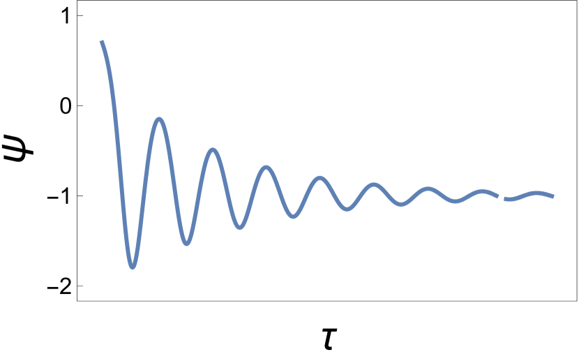
Figure 11: Coordinate dependence of the fictitious particle coordinate according to Eqs. (112), (97), (59), and (101).

Let us analyse the limiting cases of (112). Obviously, averaged kinetic energy should go to zero both when ${\cal E}\to 4$, because the period of oscillations goes to infinity, and when ${\cal E}\to-4$, because the particle approaches the bottom of the well. Equation (112) clearly demonstrates such behavior. To check it up it is enough to inspect Fig. 13 and keep in mind that

$$\lim_{k\to 0}K(k) =\lim_{k\to 0}E(k)=\frac{\pi}{2}\,,$$ (113a)

$$\lim_{k\to 1}K(k) =\infty\,,\;\;\;\;\lim_{k\to 1}E(k)=1\,.$$ (113b)

Averaged kinetic energy being found, we can easily calculate integral (59) numerically. The solution obtained in the result of the approximation is presented on Fig. 11. The shock front was not presented on purpose. The method of averaging is meaningful, provided the time scale of the change of energy is much larger than the dynamical time scale (inverse frequency of oscillations). When the energy is close to $\Pi_{w}^{(max)}$, the period of oscillation is very large, and the method ceases to be applicable.

Actually, when the method of averaging is applicable, the complicated result (112) coincides with the naive approximation (102). To show it, we plot both equations on Fig. 12. The results are close everywhere, apart from the vicinity of $\Pi_{w}^{(max)}$.

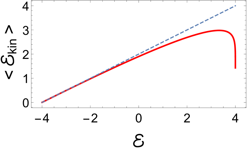
Figure 12: The averaged kinetic energy of the fictitious particle according to (112) (solid red curve) and according to (102) (dashed blue curve).

So (101) and (103) give good and simple analytic approximation to the profile of the shock wave valid everywhere, apart from the vicinity of the shock front.

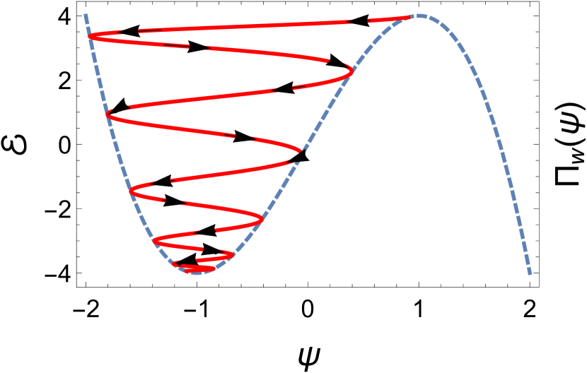
Figure 13: The particle trajectory in phase space according to Eqs. (101) and (103) (solid red curve).

Appendix D The symmetry of the modified Burgers equation

By trivial change of variables we can transform (76) to

$$u_{t}+uu_{x}+uu_{tx}=0\,.$$ (114)

To warm up, let us copy from Refs. olver ; arrigo the symmetry analysis of Burgers equation

$$u_{t}+uu_{x}=u_{xx}.$$ (115)

The symmetry group of (115) is generated by the vector field

$${\bf v}=T(t,x,u)\frac{\partial}{\partial t}+X(t,x,u)\frac{\partial}{\partial x}+U(t,x,u)\frac{\partial}{\partial u}$$ (116)

and its first and the second prolongations

$$\text{pr}^{(1)}{\bf v} ={\bf v}+U^{t}\frac{\partial}{\partial u_{t}}+U^{x}\frac{\partial}{\partial u_{x}}\,,$$ (117a)

$$\text{pr}^{(2)}{\bf v} =\text{pr}^{(1)}{\bf v}+U^{tt}\frac{\partial}{\partial u_{tt}}+U^{tx}\frac{\partial}{\partial u_{tx}}+U^{xx}\frac{\partial}{\partial u_{xx}}\,.$$ (117b)

To write down (117) explicitly, we define total derivatives

$$D_{t} =\frac{\partial}{\partial t}+u_{t}\frac{\partial}{\partial u}+u_{tt}\frac{\partial}{\partial u_{t}}+u_{tx}\frac{\partial}{\partial u_{x}}+\dots\,,$$ (118a)

$$D_{x} =\frac{\partial}{\partial x}+u_{x}\frac{\partial}{\partial u}+u_{tx}\frac{\partial}{\partial u_{t}}+u_{xx}\frac{\partial}{\partial u_{x}}+\dots\,.$$ (118b)

The coefficients of the first prolongation are

$$U^{t} =D_{t}U-u_{t}D_{t}T-u_{x}D_{t}X$$ (119a)

$$U^{x} =D_{x}U-u_{t}D_{x}T-u_{x}D_{x}X\,.$$ (119b)

The coefficients entering the second prolongation are

$$U^{tt} =D_{t}U^{t}-u_{tt}D_{t}T-u_{tx}D_{t}X\,,$$ (120a)

$$U^{tx} =D_{t}U^{x}-u_{tx}D_{t}T-u_{xx}D_{t}X\,,$$ (120b)

$$=D_{x}U^{t}-u_{tt}D_{x}T-u_{tx}D_{x}X\,,$$ (120c)

$$U^{xx} =D_{x}U^{x}-u_{tx}D_{x}T-u_{xx}D_{x}X\,.$$ (120d)

Differentiating we obtain

$$U^{t} =U_{t}+u_{t}U_{u}-u_{t}(T_{t}+u_{t}T_{u})-u_{x}(X_{t}+u_{t}X_{u})$$ (121a)

$$U^{x} =U_{x}+u_{x}U_{u}-u_{t}(T_{x}+u_{x}T_{u})-u_{x}(X_{x}+u_{x}X_{u})\,,$$ (121b)

and

$$U^{xx}=U_{xx}-u_{t}T_{xx}+u_{x}\left(2U_{xu}-X_{xx}\right)$$

$$-2u_{t}u_{x}T_{xu}+u_{x}^{2}\left(U_{uu}-2X_{xu}\right)-u_{t}u_{x}^{2}T_{uu}-u_{x}^{3}X_{uu}$$

$$-2u_{tx}T_{x}+u_{xx}\left(U_{u}-2X_{x}\right)$$

$$-2u_{x}u_{tx}T_{u}-u_{t}u_{xx}T_{u}-3u_{x}u_{xx}X_{u}.$$ (122)

Applying the second prolongation pr${}^{2}{\bf v}$ to (115) we find that $T,X,U$ must satisfy the symmetry condition

$$U^{t}+uU^{x}+u_{x}U=U^{xx}.$$ (123)

Substituting (119) and (D) eventually leads to the following set of determining equations:

$$T_{x}=0,\;\;\;T_{u}=0,\;\;\;X_{u}=0,\;\;\;U_{uu}=0,$$

$$2X_{x}-T_{t}=0,\;\;\;U_{t}+uU_{x}-U_{xx}=0,$$ (124)

$$X_{t}-X_{xx}-uX_{x}-U+2U_{xu}=0.$$

Solving the first 5 equations of (D) gives

$$X =\frac{1}{2}T^{\prime}(t)x+A(t)\,,$$ (125a)

$$U =B(t,x)u+C(t,x)\,,$$ (125b)

where $A(t)$, $B(t,x)$ and $C(t,x)$ are arbitrary functions. Substituting (125) into the remaining two equations of (D), isolating coefficients with respect to u and solving gives the infinitesimals:

$$T =c_{0}+2c_{1}t+c_{2}t^{2}\,,$$ (126a)

$$X =c_{3}+c_{4}t+c_{1}x+c_{2}tx\,,$$ (126b)

$$U =-(c_{2}t+c_{1})u+c_{2}x+c_{4}\,.$$ (126c)

Now let us come to the symmetry analysis of (114). Here we need

$$U^{tx}=U_{tx}+u_{t}(U_{xu}-T_{tx})+u_{x}(U_{tu}-X_{tx})$$

$$+u_{t}u_{x}(U_{uu}-T_{xu}-X_{xu})-u_{t}^{2}T_{xu}-u_{x}^{2}X_{tu}$$

$$-u_{t}^{2}u_{x}T_{uu}-u_{t}u_{x}^{2}X_{uu}$$

$$-u_{tt}T_{x}+u_{tx}(U_{u}-T_{t}-X_{x})-u_{xx}X_{t}$$

$$-u_{tt}u_{x}T_{u}-2u_{tx}(u_{t}T_{u}+u_{x}X_{u})-u_{t}u_{xx}X_{u}\,.$$

Applying the second prolongation pr${}^{2}{\bf v}$ to (114) we find that $T,X,U$ must satisfy the symmetry condition

$$U^{t}+uU^{x}+u_{x}U+u_{tx}U+uU^{tx}=0.$$ (128)

Substituting (119) and (D) eventually leads to the following set of determining equations:

$$T_{u}=0,\;\;\;X_{u}=0,\;\;\;X_{t}=0,\;\;\;T_{x} = 0,\;\;\;U_{uu}=0,$$

$$U_{tu}+T_{t}=0,\;\;\;U_{t}+uU_{tx}+uU_{x} = 0,$$ (129)

$$U-u^{2}U_{xu}-uX_{x} = 0\;.$$

Solving the first 5 equations of (D) gives

$$U =-T(t)u+A(x)u+B(x,t)\,,$$ (130a)

$$X =X(x)\,.$$ (130b)

Substituting (130) into the remaining two equations of (D) we obtain

$$-T^{\prime}u+B_{t}+uB_{tx}+u^{2}A^{\prime} =0\,,$$ (131a)

$$-T(t)u+A(x)u+B(x,t)-u^{2}A^{\prime}-uX^{\prime} =0\,.$$ (131b)

Isolating coefficients with respect to u and solving gives the infinitesimals:

$$T =c_{0}\,,$$ (132a)

$$X =c_{1}+c_{2}x\,,$$ (132b)

$$U =c_{2}u\,.$$ (132c)

The symmetry of the mBE turned out to be rather low. Apart from time and space translations, the only symmetry of the equation is with respect to transformation

$$u\rightarrow Cu,\;\;x\rightarrow Cx,\;\;t\rightarrow t\,.$$ (133)

This symmetry was obvious by inspection of the mBE. What was presented above, is the proof that the equation does not have any other classical symmetries. It would be interesting to check up mBE for the nonclassical symmetries.

Taking into account the symmetry of the modified Burgers equation, we may look for an exact solution of (114) in the form

$$u(x,t)=xv(t)\,.$$ (134)

Substituting (134) into (114) we obtain ordinary differential equation for $v(t)$

$$\frac{1}{v}\frac{dv}{dt}+v+\nu\frac{dv}{dt}=0\,,$$ (135)

with the solution

$$t=\frac{1}{v}-\nu\ln|v|\,.$$ (136)

Appendix E Discontinuities in the JTL with ohmic resistors in series with the JJ

Consider again the simple wave approximation for the dissipationless JTL (61). The characteristic equations for the right going wave are whitham

$$\frac{dI}{dt} =0\,,$$ (137a)

$$\frac{dx}{dt} =u(I)\,.$$ (137b)

The solution of (137) for the Cauchy problem is

$$I(x,t) =I(\xi,0)\,,$$ (138a)

$$x =\xi+u(I(\xi,0))t\,,$$ (138b)

where $I(\xi,0)$ is given by the initial condition for the problem.

Consider now the JTL with ohmic dissipation, described by (78). The characteristic equations for the right going wave are whitham

$$\frac{dI}{dt} =-\mu u^{2}(I)I\,,$$ (139a)

$$\frac{dx}{dt} =u(I)\,.$$ (139b)

Equation (139) shows that the initial value of $I(\xi,0)$ at a given point $\xi$ is propagating along the characteristic given by equation

$$x=\xi+\int_{0}^{t}u(I(\xi,t^{\prime}))dt^{\prime}\,,$$ (140)

decreasing in the process of propagation according to (139a). In (140), $I(\xi,t)$ is the solution of (139a) with the same initial condition as before.

Equation (140) (and its particular case (138b)) allow us to understand why the discontinuities in $I(x,t)$ are formed in the solution starting with the continuous initial condition $I(x,0)$. Values of current, corresponding to larger $I^{2}$ propagate slower than those corresponding to smaller $I^{2}$ (note that $u(I)/dI^{2}<0$ for all $I$), so if there are $x$ intervals, where $I^{2}(x,t)$ increases with $x$, the characteristics diverge. The discontinuities in $I(x,t)$ correspond to the crossing of the characteristic curves, that is to the existence of their envelope whitham , satisfying simultaneously (140) and equation

$$0=1+\int_{0}^{t}\left.\frac{du}{dI^{2}}\right|_{I=I(\xi,t^{\prime})}\frac{\partial I^{2}(\xi,t^{\prime})}{\partial\xi}dt^{\prime}\,.$$ (141)

The discontinuities appear at minimal $t$ for which (141) has a solution .

In the absence of ohmic dissipation, $I(\xi,t)$ is time independent, so if there are $\xi$ intervals where $I^{2}(\xi,0)$ increases with $\xi$, (141) has a solution for $t$ large enough, however small $dI^{2}(\xi,0)/d\xi>0$ is. In the presence of dissipation, the current decreases exponentially with time, so (141) has a solution only for steep enough current rises in the initial condition. Geometrically, because in the presence of dissipation the system becomes more and more linear with time, the characteristics become more and more parallel, and don’t necessarily have to cross, in distinction to the case of no dissipation.

References

- (1) G. B. Whitham, Linear and Nonlinear Waves, John Wiley & Sons Inc., New York (1999).
- (2) R. Hirota and K. Suzuki, Proc. IEEE 61, 1483 (1973).
- (3) N. S. Kuek, A. C. Liew, E. Schamiloglu, and J. O. Rossi, IEEE Trans. Dielectr. Electr. Insul. 20, 1129 (2013).
- (4) N. S. Kuek, A. C. Liew, E. Schamiloglu, and J. O. Rossi, IEEE Trans. Plasma Sci. 40, 2523 (2012).
- (5) A. Steinbrecher and T. Stykel, Int. J. Circuit Theory Appl. 41, 122 (2013).
- (6) F. S. Yamasaki, L. P. S. Neto, J. O. Rossi, and J. J. Barroso, IEEE Trans. Plasma Sci. 42, 3471 (2014).
- (7) D. M. French and B. W. Hoff, IEEE Trans. Plasma Sci. 42, 3387 (2014).
- (8) H. Fatoorehchi, H. Abolghasemi, and R. Zarghami, Appl. Math. Model. 39, 6021 (2015).
- (9) E. G. L. Rangel, J. J. Barroso, J. O. Rossi, F. S. Yamasaki, L. P. S. Neto, and E. Schamiloglu, IEEE Trans. Plasma Sci. 44, 2258 (2016).
- (10) B. Nouri, M. S. Nakhla, and R. Achar, IEEE Trans. Microw. Theory Techn. 65, 673 (2017).
- (11) L. P. S. Neto, J. O. Rossi, J. J. Barroso, and E. Schamiloglu, IEEE Trans. Plasma Sci. 46, 3648 (2018).
- (12) M. S. Nikoo, S. M.-A. Hashemi, and F. Farzaneh, IEEE Trans. Microw. Theory Techn. 66, 3234 (2018); 66, 4757 (2018).
- (13) L. C. Silva, J. O. Rossi, E. G. L. Rangel, L. R. Raimundi, and E. Schamiloglu, Int. J. Adv. Eng. Res. Sci. 5, 121 (2018).
- (14) Y. Wang, L.-J. Lang, C. H. Lee, B. Zhang, and Y. D. Chong, Nat. Comm. 10, 1102 (2019).
- (15) E. G. L. Range, J. O. Rossi, J. J. Barroso, F. S. Yamasaki, and E. Schamiloglu, IEEE Trans. Plasma Sci. 47, 1000 (2019).
- (16) A. S. Kyuregyan, Semiconductors 53, 511 (2019).
- (17) N. A. Akem, A. M. Dikande, and B. Z. Essimbi, Social Netw. Appl. Sci. 2, 21 (2020).
- (18) A. J. Fairbanks, A. M. Darr, A. L. Garner, IEEE Access 8, 148606 (2020).
- (19) R. Landauer, IBM J. Res. Develop. 4, 391 (1960).
- (20) S. T. Peng and R. Landauer, IBM J. Res. Develop. 17(1973).
- (21) R. H. Freemant and A. E. Karbowiak, J. Phys. D 10, 633 (1977).
- (22) M. I. Rabinovich and D. I. Trubetskov, Oscillations and Waves, Kluwer Academic Publishers, Dordrecht / Boston / London (1989).
- (23) B. D. Josephson, Phys. Rev. Lett. 1, 251 (1962).
- (24) A. Barone and G. Paterno, Physics and Applications of the Josephson Effect, John Wiley & Sons, Inc, New York (1982).
- (25) N. F. Pedersen, Solitons in Josephson Transmission lines, in Solitons, North-Holland Physics Publishing, Amsterda (1986).
- (26) C. Giovanella and M. Tinkham, Macroscopic Quantum Phenomena and Coherence in Superconducting Networks, World Scientific, Frascati (1995).
- (27) A. M. Kadin, Introduction to Superconducting Circuits, Wiley and Sons, New York (1999).
- (28) M. Remoissenet, Waves Called Solitons: Concepts and Experiments, Springer-Verlag Berlin Heidelberg GmbH (1996).
- (29) O. Yaakobi, L. Friedland, C. Macklin, and I. Siddiqi, Phys. Rev. B 87, 144301 (2013).
- (30) K. O’Brien, C. Macklin, I. Siddiqi, and X. Zhang, Phys. Rev. Lett. 113, 157001 (2014).
- (31) C. Macklin, K. O’Brien, D. Hover, M. E. Schwartz, V. Bolkhovsky, X. Zhang, W. D. Oliver, and I. Siddiqi, Science 350, 307 (2015).
- (32) B. A. Kochetov, and A. Fedorov, Phys. Rev. B. 92, 224304 (2015).
- (33) A. B. Zorin, Phys. Rev. Applied 6, 034006 (2016); Phys. Rev. Applied 12, 044051 (2019).
- (34) D. M. Basko, F. Pfeiffer, P. Adamus, M. Holzmann, and F. W. J. Hekking, Phys. Rev. B 101, 024518 (2020).
- (35) T. Dixon, J. W. Dunstan, G. B. Long, J. M. Williams, Ph. J. Meeson, C. D. Shelly, Phys. Rev. Applied 14, 034058 (2020)
- (36) A. Burshtein, R. Kuzmin, V. E. Manucharyan, and M. Goldstein, arXive 2010.02630v2 (2020).
- (37) B. Yurke, L. Corruccini, P. Kaminsky, L. Rupp, A. Smith, A. Silver, R. Simon, and E. Whittaker, Phys. Rev. A 39, 2519 (1989).
- (38) T. Yamamoto, K. Inomata, M. Watanabe, K. Matsuba, T. Miyazaki, W. Oliver, Y. Nakamura, and J. Tsai, Appl. Phys. Lett. 93, 042510 (2008).
- (39) M. A. Castellanos-Beltran and K. W. Lehnert, Appl. Phys. Lett. 91, 083509 (2007)
- (40) M. Hatridge, R. Vijay, D. Slichter, J. Clarke, and I. Siddiqi, Phys. Rev. B 83, 134501 (2011).
- (41) B. Abdo, F. Schackert, M. Hatridge, C. Rigetti, and M. Devoret, Appl. Phys. Lett. 99, 162506 (2011).
- (42) J. Mutus et al., Appl. Phys. Lett. 103, 122602 (2013).
- (43) C. Eichler, Y. Salathe, J. Mlynek, S. Schmidt, and A. Wallraff, Phys. Rev. Lett. 113, 110502 (2014).
- (44) T. C. White et al., Appl. Phys. Lett. 106, 242601 (2015).
- (45) A. Miano and O. A. Mukhanov, IEEE Trans. Appl. Supercond. 29, 1501706 (2019).
- (46) Ch. Liu, Tzu-Chiao Chien, M. Hatridge, D. Pekker, Phys. Rev. A 101, 042323 (2020).
- (47) G. J. Chen and M. R. Beasley, IEEE Trans. Appl. Supercond. 1, 140 (1991).
- (48) H. R. Mohebbi and A. H. Majedi, IEEE Trans. Appl. Supercond. 19, 891 (2009); IEEE Transactions on Microwave Theory and Techniques 57, 1865 (2009).
- (49) H. Katayama, N. Hatakenaka, and T. Fujii, Phys. Rev. D 102, 086018 (2020).
- (50) M. B. Vinogradova, O. V. Rudenko and A. P. Sukhorukov, The Wave Theory, Nauka Publishers, Moscow (1990).
- (51) N. Kwidzinski and R. Bulla, arXive1608.0061.
- (52) M. Abramowitz, I. A. Stegun eds., Handbook of Mathematical Functions with Formulas, Graphs, and Mathematical Tables, (National Bureau of Standards, Washington, 1964).
- (53) A. P. Prudnikov, Yu. A. Brychkov and O. I. Marichev, Integrals and Series Vol. 2 (Gordon and Breach Science Publishers, 1986).
- (54) P. M. Marcus, Y.Imry, and E. Ben-Jacob, Solid State Comm. 41, 161 (1982).
- (55) U. Kruger, J. Kurkijarvi, M. Bauer, and W. Martienssen, Chaos and Nonlinear Effects in Josephson Junctions and Devices, in Nonlinear Dynamics in Solids, Springer-Verlag Berlin Heidelberg New York (1992).
- (56) K. L. Likharev, Dynamics of Josephson Junctions and Circuits, Gordon and Breach Science Publishers, New York, NY (1986).
- (57) R. Eichhorn, S. J. Linz, and P. Hanggi, Chaos, Solitons & Fractals, 13, 1 (2002).
- (58) J. C. Sprott, Elegant Chaos, World Scientific, Singapore (2010).
- (59) J. Billingham and A. C. King, Wave Motion, Cambridge University Press, Cambridge (2000).
- (60) T. H. A. van der Reep, Phys. Rev. A 99, 063838 (2019).
- (61) L Fasolo, A Greco, E Enrico, in Advances in Condensed-Matter and Materials Physics: Rudimentary Research to Topical Technology, (ed. J. Thirumalan and S. I. Pokutny), Sceence (2019).
- (62) A. Greco, L. Fasolo, A. Meda, L. Callegaro, and E. Enrico, arXiv:2009.01002.
- (63) Y. Yuan, M. Haider, J. A. Russer, P. Russer and C. Jirauschek, 2020 XXXIIIrd General Assembly and Scientific Symposium of the International Union of Radio Science, Rome, Italy (2020).
- (64) E. Bettelheim1 and L. I. Glazman, Phys. Rev. Lett. 109, 260602 (2012).
- (65) Th. Veness and L. I. Glazman, Phys. Rev. B 100, 235125 (2019).
- (66) I.S. Gradshteyn and I.M. Ryzhik, Table of Integrals, Series, and Products, Elsevier Inc., Amsterdam (2007).
- (67) E. Goursat, Course d’analyse mathematique, Tome I, Gautier-Villars, Paris (1933).
- (68) P. J. Olver, Application of Lie groups to Differential Equations, Springer-Verlag Ney York, Inc. (1993).
- (69) D. J. Arrigo, Symmetry Analysis of Differential Equations, John Wiley & Sons, Inc., Hoboken, NJ (2015).