Trends in COVID-19 prevalence and mortality: a year in review

Abstract

This paper introduces new methods to study the changing dynamics of COVID-19 cases and deaths among the 50 worst-affected countries throughout 2020. First, we analyse the trajectories and turning points of rolling mortality rates to understand at which times the disease was most lethal. We demonstrate five characteristic classes of mortality rate trajectories and determine structural similarity in mortality trends over time. Next, we introduce a class of virulence matrices to study the evolution of COVID-19 cases and deaths on a global scale. Finally, we introduce three-way inconsistency analysis to determine anomalous countries with respect to three attributes: countries’ COVID-19 cases, deaths and human development indices. We demonstrate the most anomalous countries across these three measures are Pakistan, the United States and the United Arab Emirates.

1 Introduction

2020 will be remembered as the year that the world first battled the COVID-19 pandemic. Almost 2 million people lost their lives, substantial restrictions on population movement and activities were imposed, and almost every country experienced an economic recession. During that year, treatments improved substantially [1, 2, 3, 4] and several vaccines were produced by the end of the year [5, 6]. However, the disease remains highly prevalent around the world as of the start of 2021, and measures to contain and reduce its transmission remain highly relevant for the reduction of casualties as well as economic and other social consequences [7, 8].

Throughout the year, government responses to the pandemic varied substantially, both over time and between countries. Early government responses included banning travel [9], the implementation of testing and contact tracing programs [10], and lockdowns. Due to the economic consequences of lockdowns, many countries implemented them too late [11, 12] and lifted restrictions before cases had sufficiently reduced [13]. Such disparate responses to the virus led to great variability in case and death counts, creating different waves of the outbreak across many countries. Such later waves often exhibited higher case and death counts than the first [14, 15].

The response of the scientific community to COVID-19 has also been varied and multifaceted, producing research from many perspectives and disciplines. In addition to the aforementioned medical research [1, 2, 3, 4, 5, 6], mathematical approaches to model and analyse the virus and its impact have been broad. First, models based on existing statistical techniques, such as the Susceptible–Infected–Recovered (SIR) model and the basic reproductive ratio $R_{0}$, have been proposed and systematically collated by researchers [16, 17]. These have been used for various purposes, including diagnosis and prognosis of COVID-19 patients, efficacy of medications, and vaccine development. Next, nonlinear dynamics researchers have proposed several sophisticated extensions to the classical predictive SIR model, including analytic techniques to find explicit solutions [18, 19], modifications to the SIR model with additional variables [20, 21, 22, 23, 24], incorporation of Hamiltonian dynamics [25] or network models [26] and a closer analysis of uncertainty in the SIR approach [27]. Other mathematical approaches to prediction and analysis include power-law models [28, 29, 30], distance analysis [31, 32], network models [33, 34, 35, 36], analyses of the dynamics of transmission and contact [37, 38], forecasting models [39], Bayesian methods [40], clustering [41, 42] and many others [43, 44, 45, 46].

We have a different motivation and approach relative to the aforementioned work. Rather than performing predictions on an individual country basis or comparing parameters among different countries (such as $R_{0}$ or power-law exponents), we seek to reveal structural similarity in COVID-19 case, death and mortality time series across many countries of the world. Rather than predicting the future, which is always challenging due to unpredictable changes in government policy, we aim to be descriptive, revealing similarity and anomalous countries in outcomes. Indeed, close analysis of the case, death and mortality dynamics on a country-by-country basis is necessary to inform governments of the most successful strategies for reducing transmission of cases and progression to deaths. Identifying structural similarities between countries’ trajectories can support conclusions that certain government responses will likely result in better or worse outcomes. Moreover, identifying anomalous countries can provide insights on which responses to the pandemic were exceptionally good or poor. For this purpose, we present three sections, each of which contributes a new mathematical method for analysing the world’s COVID-19 cases, deaths and mortality, or any multivariate time series more generally.

This paper is therefore structured as follows. In Section 2, we analyse the trajectories of mortality rates on a country-by-country basis. In particular, we build upon a recently introduced algorithmic framework to identify the turning points of the mortality trajectories, which reveal when the disease was most and least lethal (with respect to the progression from cases to deaths). We then use a new semi-metric between finite sets to assign countries into classes of mortality trajectories. We believe this is the first work to classify different mortality trajectories among countries, rather than a more traditional comparison of overall mortality rates without considering its changing dynamics over time. In Section 3, we analyse the eigenspectra of virulence matrices as a new means of understanding trends in the worldwide prevalence and mortality of COVID-19. This reveals periods in which COVID-19 was most severe and most heterogeneous between countries. In Section 4, we compare countries’ case and death counts with their human development index (HDI) and use a new method to identify the most anomalous countries between these attributes. In Section 5, we discuss our findings from the aforementioned analyses regarding COVID-19 trends throughout the year 2020. We conclude in Section 6.

2 Mortality rate analysis

In this section, we study the dynamics of the COVID-19 mortality rate among $n=50$ countries. Our data spans 01/01/2020 to 31/12/2020, a period of $T=366$ days. We choose the countries with the 50 greatest total case counts of COVID-19 as of 31/12/2020, order these by alphabetical order, and index them $i=1,...,n$. Let $x_{i}(t),y_{i}(t)\in\mathbb{R}$ be the multivariate time series of new daily cases and deaths, respectively, for $i=1,...,n$ and $t=1,...,T$. Throughout this paper, the subscript $i$ pertains to the $i$th country, ordered alphabetically, while evaluating a function at $t$ gives its value at the $t$th day of the year. For a given country, let $r_{i}(t)$ be its 30-day rolling mortality rate, defined by

$$r_{i}(t)=\dfrac{\sum_{s=t-29}^{t}y_{i}(s)}{\sum_{s=t-29}^{t}x_{i}(s)},t=30,...,T,$$ (1)

or zero if no cases have been observed over the last 30 days. This gives a multivariate time series $r_{i}(t)$, for $i=1,...,n$ and $t=30,...,T$. The data point at time $t$ describes the rolling mortality rate over the prior 30 days.

2.1 Methodology

The aim of this section is to study these mortality trends on a country-by-country basis and identify structural similarity across different countries. For this purpose, we use two (semi)-metrics between the mortality rate time series and apply hierarchical clustering [47, 48] to these measures. Hierarchical clustering has been used in several epidemiological applications, including inflammatory diseases [49], airborne diseases [50], Alzheimer’s disease [51], Ebola [52], SARS [53], and COVID-19 [41].

These mortality rates $r_{i}(t)$ exhibit highly undulating behaviour, moving between clear peaks and troughs (turning points). Our first semi-metric measures distance between algorithmically-identified turning points as a proxy for each time series’ behaviour. We modify an existing algorithmic framework for this purpose. First, we apply a Savitzky-Golay filter to produce a collection of smoothed time series $\hat{r}_{i}(t)$, $t=30,...,T$ and $i=1,...,n$. A beneficial effect of this smoothing is to ameliorate some of the noise present in the COVID-19 case count data. In addition to the smoothing procedure, our computation includes a rolling mortality rate that further reduces the effect of perturbations in the data’s underlying signal. We choose a 30-day rolling mortality rate for two reasons: first, this window length provides a compromise between denoising the data and not over-smoothing; second, 30 days provides a good luck at the mortality rate behaviour of the last month of data. Next, we follow [15] and apply a two-step algorithm where we select and then refine a set of turning points. We assign each smoothed mortality rate time series a non-empty set $P_{i}$ and $T_{i}$ of local maxima (peaks) and local minima (troughs). To better suit our specific application, we modify the second step of this algorithm, in which the turning point list is refined. Full details are included in A, including a discussion of the procedure’s robustness against noisy data. We display 12 countries’ mortality rate time series and annotate their turning points in Figure 1.

To quantify distance between time series’ turning points, we modify the semi-metric of [32] (with $p=1$). Given two non-empty finite sets $S_{1},S_{2}\subset\{1,2,...,T\}$, this is defined as

$$D({S_{1}},{S_{2}})=\frac{1}{2T}\left(\frac{\sum_{b\in S_{2}}d(b,S_{1})}{\#S_{2}}+\frac{\sum_{a\in{S_{1}}}d(a,S_{2})}{\#S_{1}}\right),$$ (2)

where $d(b,S_{1})$ is the minimal distance from $b\in S_{2}$ to the set $S_{1}$, and $\#S_{1}$ is the cardinality of $S_{1}$, and analogously for $S_{2}$. By the choice of normalisation, this is always bounded between 0 and 1. To more appropriately separate different behaviours among mortality trends, we modify this semi-metric by including a regularisation term. This treatment is inspired by various regularisation penalties in the statistical literature [54]. We construct our semi-metric as follows:

$$D^{\prime}({S_{1}},{S_{2}})=D(S_{1},S_{2})+\beta|\#S_{1}-\#S_{2}|,$$ (3)

where $0<\beta\leq 1$ is a constant. The resulting values $D^{\prime}(S_{1},S_{2})$ are symmetric, non-negative, and zero if and only if $S_{1}=S_{2}$. Then, we define the $n\times n$ matrix $D^{TP}$ between turning point sets by

$$D_{ij}^{TP}=D^{\prime}(P_{i},P_{j})+D^{\prime}(T_{i},T_{j}).$$ (4)

Here, $P_{i}$ denotes the set of peaks for the $i$th country’s mortality series, while the subscript $ij$ gives a distance between countries $i$ and $j$, ordered alphabetically. In Figure 2, we perform hierarchical clustering on $D^{TP}$ with a range of values of $\beta$. These distances do not capture the absolute values of the mortality rate time series; they only distinguish between their undulating behaviour, reflected in their sets of turning points. To round out our analysis, we include another metric, an $L^{1}$ norm that does account for difference in the absolute values of mortality. We define another matrix by

$$D_{ij}^{1}=\sum_{t=30}^{T}|r_{i}(t)-r_{j}(t)|,$$ (5)

and perform hierarchical clustering on $D^{1}$ in Figure 3. Again, the subscript $ij$ refers to a distance computed between countries $i$ and $j$, ordered alphabetically.

2.2 Results

In Figure 1, we display rolling mortality rate and turning points for 12 countries: Brazil, India, Mexico, the United States (US), the Netherlands, Sweden, France, Germany, Italy, Russia, Ecuador and Bulgaria. These countries display highly heterogeneous behaviours, which are suitably captured in Figure 2. Figure 2(a) reveals four clusters of similarity, and one outlier. Russia (1(j)) is the unique country with just two detected turning points. Several developing countries such as Brazil (1(a)), India (1(b)) and Mexico (1(c)) as well as developed countries including the US (1(d)), the Netherlands (1(e)) and Sweden (1(f)) have three turning points. France (1(g)), Germany (1(h)) and Italy (1(i)) have four turning points. Ecuador (1(k)) and others have five, while Bulgaria (1(l)) and others have six. Figure 2(b) gives a near-identical result, where the clusters pertaining to five and six turning points merge. However, examining the dendrogram closely, both are clearly visible as subclusters, and we are comfortable identifying five categories of trajectories. To demonstrate the robustness of our method, we record the cluster structure for a greater range of $\beta$ in Table 1.

Within the 4-turning point cluster, we see a dense subcluster of similarity containing Austria, Belgium, Canada, Czechia, France, Georgia, Germany, Hungary, Italy, Poland, Portugal, Switzerland and the United Kingdom (UK). All these countries experienced a peak in the mortality rate in April or May (corresponding to the previous 30 days) and a local minimum near the beginning of September (corresponding to the previous 30 days during August). This similarity can be seen by examining members of this cluster, France (1(g)), Germany (1(h)) and Italy (1(i)).

Turning to Figure 3, several other insights concerning the mortality rate trajectories emerge. First, Mexico and Ecuador are identified as outliers in the collection of countries, with only slight similarity to each other. For Mexico (1(c)), this is due to a consistently high mortality rate over time, over 10% for most of the period. Ecuador (1(k)) is an outlier due to peaks in mortality over 30%, higher than any other country. Belgium, France, Hungary, Spain, and the UK form their own smaller cluster characterised by high mortality rates (of around 20%) in their first wave of COVID-19. Indeed, these countries experienced higher mortality in March-April than anywhere else in the world.

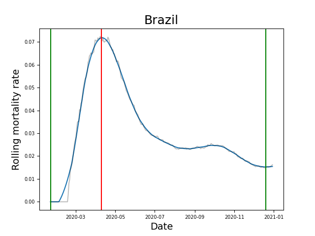
(a)

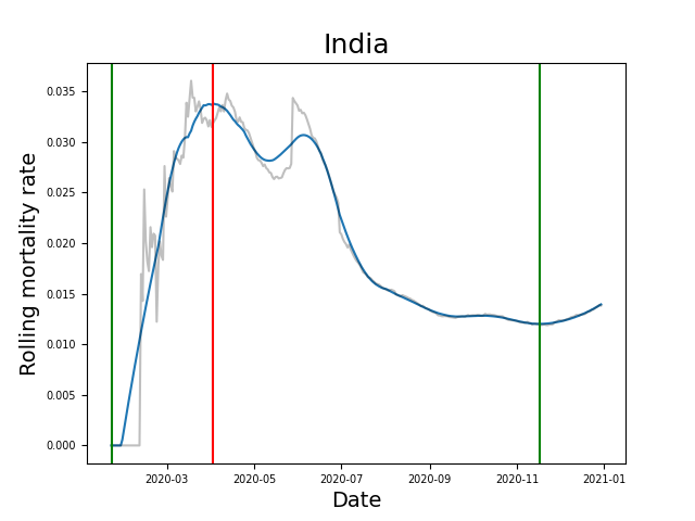
(b)

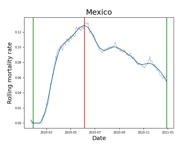
(c)

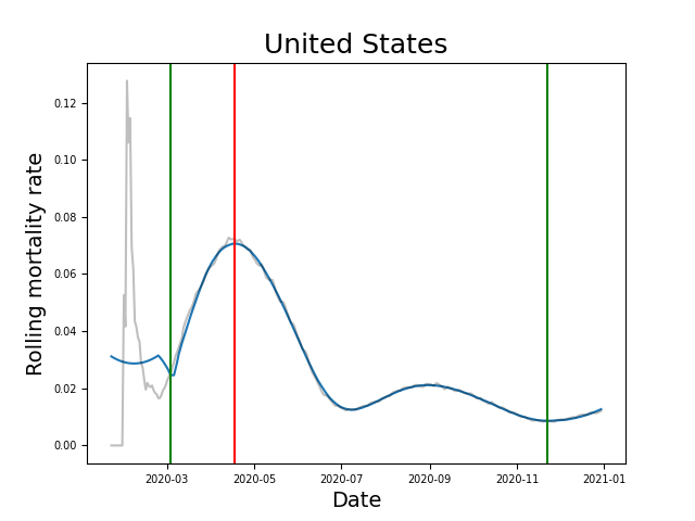
(d)

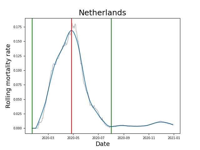
(e)

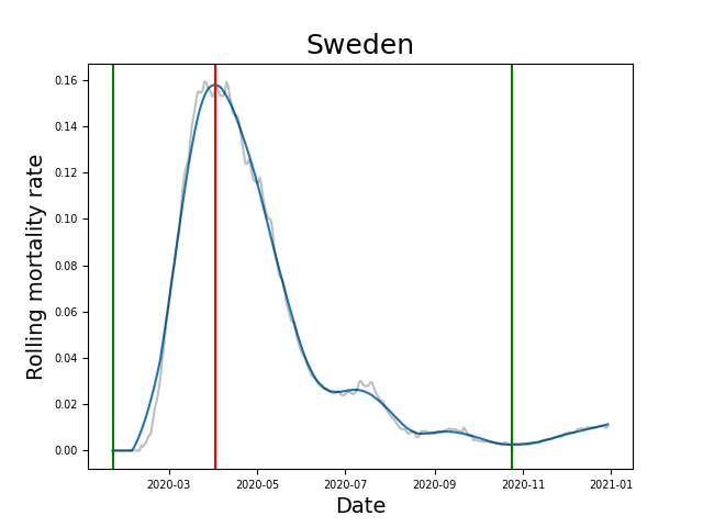
(f)

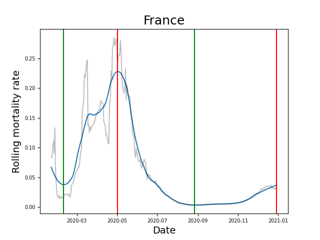
(g)

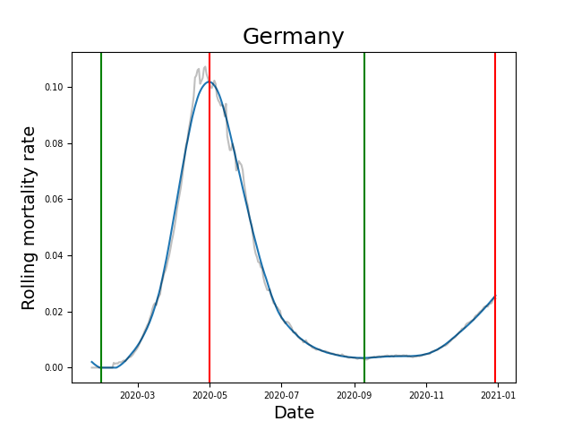
(h)

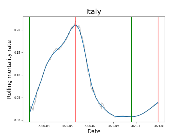
(i)

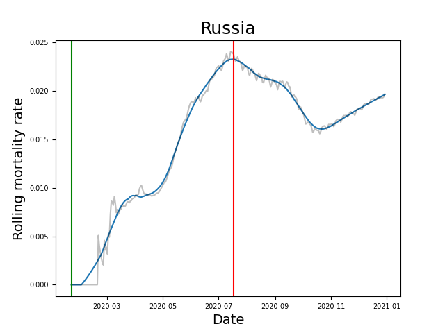
(j)

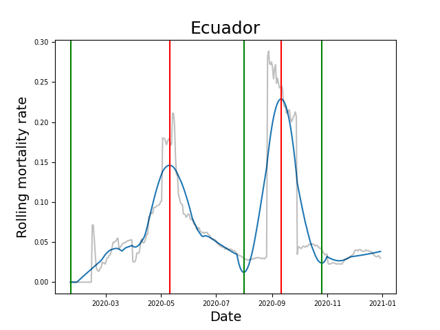
(k)

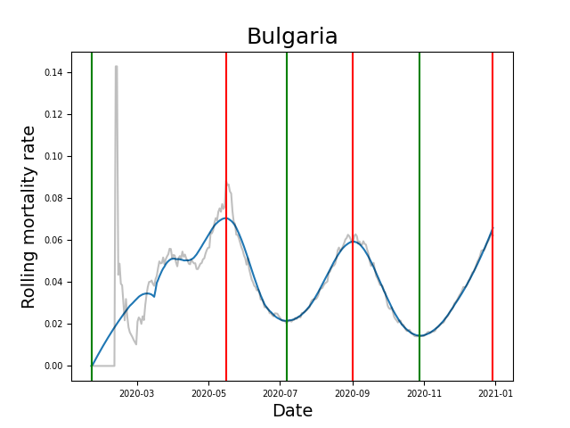
(l)

Figure 1: Smoothed mortality rate time series and identified turning points for various countries: (a) Brazil (b) India (c) Mexico (d) the US (e) the Netherlands (f) Sweden (g) France (h) Germany (i) Italy (j) Russia (k) Ecuador (l) Bulgaria. Green and red vertical lines denote algorithmically detected troughs and peaks, respectively. The rolling mortality rate at a given time calculates the mortality over the previous 30 days. The aforementioned countries represent at least one member of every characteristic class of trajectories.

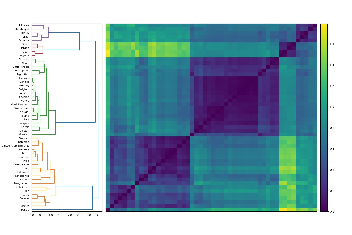
(a)

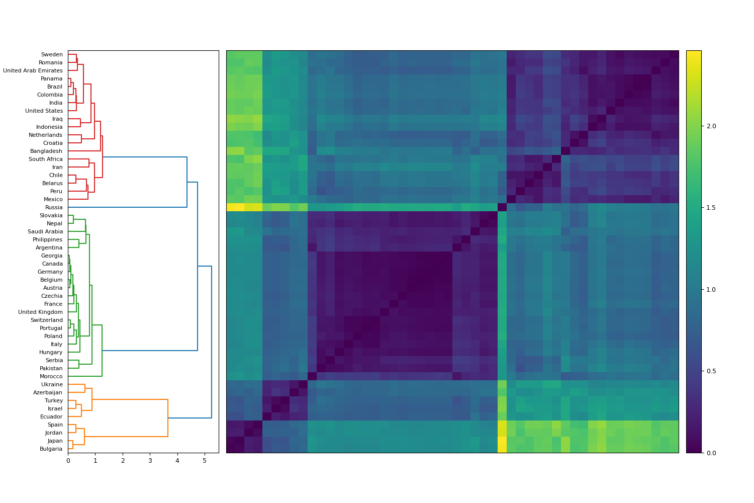
(b)

Figure 2: Hierarchical clustering on the turning point distance matrix $D^{TP}$, defined in Section 2, for (a) $\beta=1/3$, (b) $\beta=1/2$. This groups countries according to their similarity in undulating behaviour, measured by distances between turning point sets. Five characteristic classes are observed: Russia has two turning points; Brazil, India and the US have three; most European countries have four, with a strong subcluster of similarity observed including Austria, Belgium, and others. Two smaller classes are observed containing five and six turning points, respectively. The cluster structure in the two dendrograms is near identical, with a consolidation of the five- and six-turning point classes in (b). There, these classes are clearly observed as subclusters.

Cluster robustness vs $\beta$
$\beta$	# Clusters	Cluster sizes
1/5	4	{21,19,9,1}
1/4	4	{21,19,9,1}
1/3	5	{21,19,5,4,1}
1/2	4	{21,19,9,1}
1	4	{21,19,9,1}

Table 1: Number of clusters and cluster sizes for different values of the parameter $\beta$, used to define the semi-metric in Eq. (3). While a different number of clusters is observed for $\beta=1/3$, subclusters with 5 and 4 elements are clearly visible in Figure 2(a).

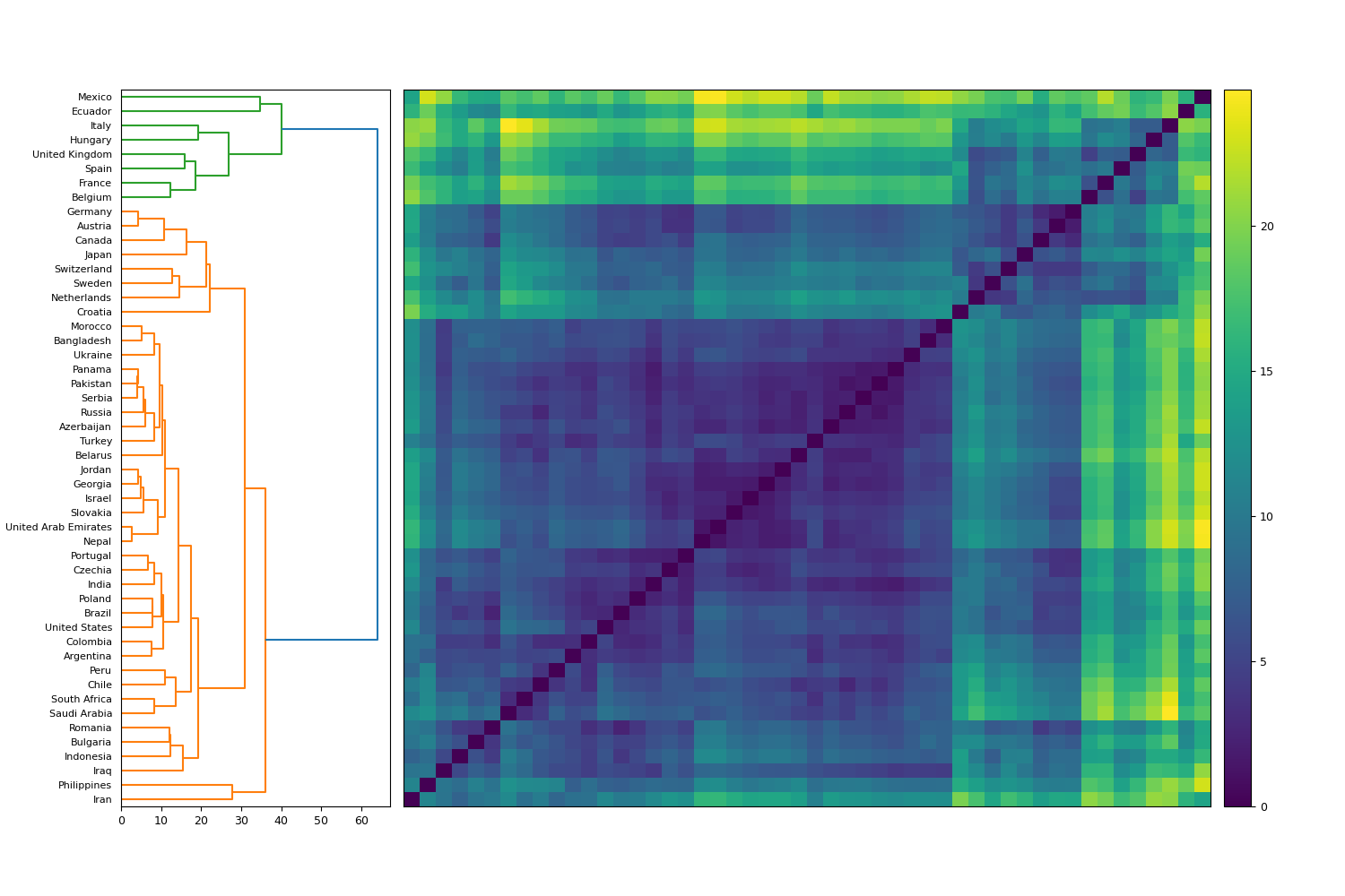
Figure 3: Hierarchical clustering on the $L^{1}$ distance matrix $D^{1}$, defined in Section 2. Mexico and Ecuador emerge as outliers, characterised by a consistently high mortality rate over the full period and the highest peaks in mortality of all, respectively. Belgium, France, Hungary, Spain and the UK are revealed as a secondary cluster, characterised by high mortality in April and May, rapidly decreasing from then.

3 Virulence matrix analysis

In this section, we develop a new framework of time-varying analysis of 30-day rolling virulence matrices, inspired by, but differing from, covariance matrices in finance [55]. Let $t=30,...,T$ be a particular time. We form vectors $\mathbf{x}_{i}(t)=(x_{i}(t-29),...,x_{i}(t))$, analogously for $\mathbf{y}_{i}$(t). These two vectors record the case and death counts over the past 30 days, with the subscript $i$ referring to the $i$th country, ordered alphabetically. We may also form $\mathbf{r}_{i}(t)=(r_{i}(t-29),...,r_{i}(t))$ for $t=59,...,T$, as the time series $r_{i}(t)$ only begin at $t=30$. Define (unscaled) inner products by

$$\langle\mathbf{x}_{i}(t),\mathbf{x}_{j}(t)\rangle=\sum_{s=t-29}^{t}x_{i}(s)x_{j}(s).$$ (6)

We then define $n\times n$ (unscaled) virulence matrices with respect to cases, deaths and mortality rates by the following $(i,j=1,...n)$:

$$V_{ij}^{c}(t) =\langle\mathbf{x}_{i}(t),\mathbf{x}_{j}(t)\rangle,t=30,...,T;$$ (7)

$$V_{ij}^{d}(t) =\langle\mathbf{y}_{i}(t),\mathbf{y}_{j}(t)\rangle,t=30,...,T;$$ (8)

$$V_{ij}^{r}(t) =\langle\mathbf{r}_{i}(t),\mathbf{r}_{j}(t)\rangle,t=59,...,T.$$ (9)

The subscript $ij$ refers to an inner product between the $i$th and $j$th countries, while the superscripts $c,d,r$ refer to case, death and mortality rate time series, respectively. Due to the summation procedure used to form these inner products, these virulence matrices implicitly average over 30 days’ worth of case counts and can are thus robust against the noise present in day-to-day data. We could also analogously define normalised virulence matrices by using normalised inner products in place of the unscaled inner products above. These matrices are thus named because they provide a representation of the global spread of COVID-19 over the last 30 days and contain relationships between different countries’ trajectories. The use of a standard covariance matrix here would not appropriately measure this prevalence: a country with a constant (but severe) number of cases for the past 30 days would yield a zero covariance with any other country. Each matrix $V(t)$ is a $n\times n$ symmetric real matrix, and thus is diagonalisable with all real eigenvalues. By the positivity of the inner product, each matrix satisfies a non-negativity condition $\mathbf{u}^{T}V\mathbf{u}\geq 0$ for $\mathbf{u}\in\mathbb{R}^{n}$, and so all eigenvalues are non-negative. We list and order the eigenvalues $\lambda_{1}\geq\lambda_{2}\geq...\geq\lambda_{n}\geq 0$. This produces a time-varying eigenspectrum, which we display in Figure 4 for the first ten eigenvalues. Moreover, for any such symmetric matrix, the greatest eigenvalue $\lambda_{1}$ holds particular significance. By the spectral theorem, $\lambda_{1}$ coincides with the operator norm of the matrix [56], a measure of its total size. That is,

$$\lambda_{1}=||V||_{op}=\max_{\mathbf{u}\in\mathbb{R}^{n}-\{0\}}\frac{||V\mathbf{u}||}{||\mathbf{u}||}.$$ (10)

Subsequent eigenvalues also have a real-world interpretation. $\lambda_{2}=0$ if and only if the matrix $V$ is rank 1, which occurs if and only if all trajectories $\mathbf{x}_{i}$ (in the instance of the cases matrix) differ by a multiplicative constant. In general, a small value of $\lambda_{2}$ relative to $\lambda_{1}$ indicates substantial homogeneity in the trajectories.

In Figures 4(a), 4(b) and 4(c), respectively, we display the time-varying eigenspectra for the virulence matrices associated to cases, deaths and mortality rates. There are several interesting properties of these time-varying eigenspectra. The first eigenvalue $\lambda_{1}$ of Figure 4(a) demonstrates the general increase of new COVID-19 cases over the course of 2020. The sharp spike towards the end of the year demonstrates the rapid growth in cases in the final months of 2020. Figure 4(b) has two prominent peaks in its first eigenvalue, corresponding to the periods of March-April and November-December. These peaks highlight the natural history of COVID-19, where many countries suffered significant deaths during their first wave of the virus, enforced harsh restrictions resulting in fewer cases and deaths, and subsequently experienced further growth in cases and deaths upon such restrictions’ easing. Finally, the first eigenvalue in Figure 4(c) highlights an interesting trend in the mortality rate. There is a marked spike in March-April, followed by a significant reduction throughout the remainder of 2020. This shape in the first eigenvalue likely represents vulnerable people dying earlier and/or under-reporting of cases early in the year, contributing to a higher calculated mortality rate from reported cases and deaths.

The relationship between the first eigenvalue and subsequent eigenvalues is also of interest. Figure 4(a) shows the second eigenvalue $\lambda_{2}$ becoming quite significant for cases towards the end of 2020, when the total number of cases is larger than ever. This shows that the behaviour of new cases in late 2020 is more heterogeneous than the first wave, when all cases were rising quite uniformly throughout the world. Figures 4(b) and 4(c) show a more moderate, but similar phenomenon concerning deaths and mortality rate at various stages of the year. The second eigenvalue in Figure 4(b) is slightly more pronounced in the second wave of the virus, displaying more heterogeneity in COVID-19 deaths later in the year. The second eigenvalue in Figure 4(c) is more pronounced during the first wave of the virus - highlighting more heterogeneity during the first wave of the virus with respect to mortality. Indeed, Figure 1 shows that European countries experienced substantial mortality in their first wave of COVID-19, which characterised them as anomalous in Figure 3. This contributed to a meaningful heterogeneity of mortality rates across the world during the early stages of the year.

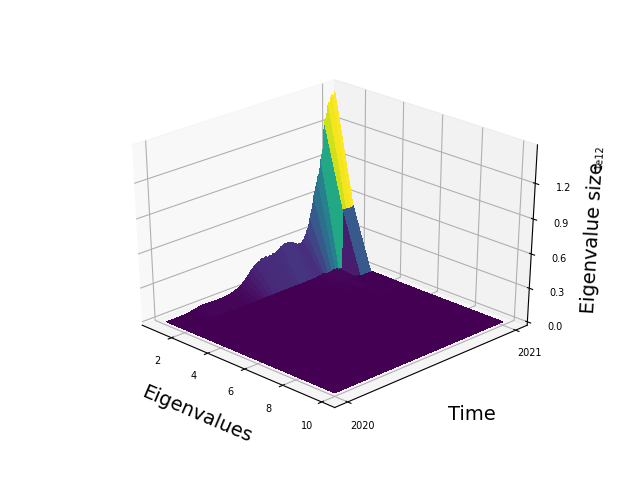
(a)

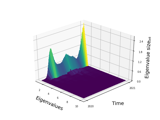
(b)

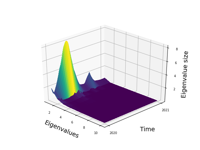
(c)

Figure 4: Time-varying eigenspectra (first ten eigenvalues) for the virulence matrices associated to (a) cases (b) deaths (c) mortality rate. The first eigenvalue demonstrates broad trends in the total size of the matrices, and shows (a) a large increase of cases towards the end of 2020, (b) two or three waves of significant deaths, (c) the highest mortality early on in the year. The second eigenvalue reveals more heterogeneity in case trajectories towards the end of the year, and mortality towards the beginning of the year.

4 Inconsistency analysis

In this section, we describe how we measure the consistency between three attributes, and reveal anomalous countries in the process. To do so, we introduce a new method of comparing three distance matrices and apply this to distances between case and death time series, and human development indices (HDI). This generalises prior work studying anomalies between two attributes [57].

4.1 Methodology

Let $h_{i}$ be the HDI of each country. Calculated by the United Nations Development Programme [58], this index combines a country’s life expectancy, educational standards and economic standard of living. Bounded between 0 and 1, the HDI $h_{i}$ reflects a substantially lower living standard the further $h$ moves from 1. To reflect this, we use a logarithmic distance between these indices that penalises movement away from 1 more than a linear distance:

$$D_{ij}^{h} =|\log h_{i}-\log h_{j}|,i,j=1,...,n.$$ (11)

As before, the subscript $i$ refers to the $i$th country, ordered alphabetically, the subscript $ij$ refers to a distance between the $i$th and $j$th country, while the superscript $h$ signals a distance relative to HDI. This forms a $n\times n$ distance matrix between countries’ development indices. Given the exponential nature of the spread of the virus, we also use a logarithmic distance between the case and death time series. Some of these time series have negative counts due to retrospective adjustments in the data. In order to ensure non-negative counts, we first apply a Savitzky-Golay filter to produce smoothed case and death time series $\hat{x}_{i}(t)$ and $\hat{y}_{i}(t)$ respectively. Due to its moving average and polynomial smoothing, this eliminates almost all negatives, except when there are very few counts. We replace any non-positive count with a 1. Then, we may calculate a logarithmic $L^{1}$ distance as follows:

$$D_{ij}^{c} =||\log\hat{x}_{i}-\log\hat{x}_{j}||=\sum_{t=1}^{T}|\log\hat{x}_{i}(t)-\log\hat{x}_{j}(t)|;$$ (12)

$$D_{ij}^{d} =||\log\hat{y}_{i}-\log\hat{y}_{j}||=\sum_{t=1}^{T}|\log\hat{y}_{i}(t)-\log\hat{y}_{j}(t)|.$$ (13)

Above, the superscripts $c,d$ refer to distances relative to the case and death time series, respectively, between countries $i$ and $j$. Again, the summation across many days of data has the effect of smoothing out over the noise inherent in day-to-day variations of case counts. We use such a metric between case or death time series rather than a simple difference between the total yearly counts to distinguish between countries (and hence reveal potential anomalies) according to when the cases or deaths occurred. Thus, we have defined three $n\times n$ distance matrices between countries. Given a $n\times n$ distance matrix $D$, its corresponding affinity matrix is defined as

$$A_{ij}=1-\frac{D_{ij}}{\max{\{D\}}},i,j=1,...,n.$$ (14)

All elements of these affinity matrices lie in $[0,1]$, so it is appropriate to compare them directly by taking their difference. Given a $n\times n$ matrix $C$, let $|C|$ be the matrix given by taking the absolute value of all elements, that is $|C|_{ij}=|C_{ij}|$. Then, define three $n\times n$ symmetric pairwise inconsistency matrices:

$$\text{INC}^{c,d} =|A^{c}-A^{d}|;$$ (15)

$$\text{INC}^{c,h} =|A^{c}-A^{h}|;$$ (16)

$$\text{INC}^{d,h} =|A^{d}-A^{h}|;$$ (17)

and a total inconsistency matrix

$$\text{INC}^{c,d,h}=\text{INC}^{c,d}+\text{INC}^{c,h}+\text{INC}^{d,h}.$$ (18)

Above and below, a superscript $c,d$ refers to inconsistency between cases and deaths, while $c,h$ refers to an inconsistency between cases and HDI, and similarly for $d,h$. A superscript $c,d,h$ refers to an inconsistency between all three attributes. Next, we can define pairwise anomaly scores by

$$a_{i}^{c,d} =\sum_{j=1}^{n}\text{INC}_{ij}^{c,d};$$ (19)

$$a_{i}^{c,h} =\sum_{j=1}^{n}\text{INC}_{ij}^{c,h};$$ (20)

$$a_{i}^{d,h} =\sum_{j=1}^{n}\text{INC}_{ij}^{d,h}.$$ (21)

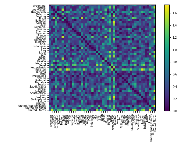
Figure 5: Total anomaly matrix $\text{INC}^{c,d,h}$, as defined in Section 4. Lighter entries indicate higher values of the matrix, and hence more inconsistency between the attributes under consideration: cases, deaths and HDI. The US and Pakistan can be seen to have substantial inconsistency with many other countries.

For each country, we record an anomaly vector $\mathbf{a}_{i}=(a_{i}^{c,d},a_{i}^{c,h},a_{i}^{d,h})$ and a total anomaly score given by $a_{i}^{c,d,h}=a_{i}^{c,d}+a_{i}^{c,h}+a_{i}^{d,h}$. We can also define a weighted anomaly score to reduce bias in one set of anomaly scores being systematically larger than another. Let $M^{c,d}=\max_{i}\{a_{i}^{c,d}\}$, analogously for $M^{c,h}$ and $M^{d,h}$. Let the weighted anomaly score be $\tilde{a}_{i}^{c,d,h}=a_{i}^{c,d}/M^{c,d}+a_{i}^{c,h}/M^{c,h}+a_{i}^{d,h}/M^{d,h}$. This aims to record a neutral contribution from each anomaly score. In Tables 2 and 3, we record the anomaly vectors, total anomaly score and weighted anomaly score for all 50 countries under consideration. In Figure 5, we plot the total consistency matrix $\text{INC}^{c,d,h}$, where anomalous countries can easily be seen due to larger entries in their respective rows and columns. An analogous weighted consistency matrix can also be defined, which is broadly similar to the one shown.

Remark 4.1.

In this brief aside, we explore the edge cases of maximal consistency and maximal inconsistency, and interpret their meaning. Consider a single entry $\text{INC}^{c,d}_{ij}=|A^{c}_{ij}-A^{d}_{ij}|$. As both $A^{c}_{ij},A^{d}_{ij}\in[0,1]$, the inconsistency entry $\text{INC}^{c,d}_{ij}$ has greatest possible value to 1. It attains that value when $A^{c}_{ij}=1$ and $A^{d}_{ij}=0$, or vice versa. This equations can be reinterpreted as $D^{c}_{ij}=0$ and $D^{d}_{ij}=\max D^{d}$, respectively. That is, greatest inconsistency occurs when countries $i$ and $j$ have equal case counts, but the greatest difference in death counts among any pair of countries, or vice versa. The exact same statement applies for greatest inconsistency between cases and HDI or deaths and HDI.

On the other hand, greatest possible consistency across the entire matrix would mean $A^{c}_{ij}-A^{d}_{ij}=0$, for all $i,j$. Rearranging this yields $\frac{D^{c}_{ij}}{\max D^{c}}=\frac{D^{d}_{ij}}{\max D^{d}}$, for all $i,j$. That is, the distance matrices $D^{c}$ and $D^{d}$ differ up to a single scalar. One example where this can occur is if there are constants $a$ and $\tau$ such that $y_{i}(t)=ax_{i}(t+\tau)$, for all $i=1,...,n,t=1,...,T$. Then this relationship passes to the smoothed counts by linearity, and so $\sum_{t}|\log\hat{y}_{i}(t)-\log\hat{y}_{j}(t)|=\sum_{t}|\log a\hat{x}_{i}(t+\tau)-\log a\hat{x}_{j}(t+\tau)|=\sum_{t}|\log\hat{x}_{i}(t)-\log\hat{x}_{j}(t)|$. That is, maximal consistency would occur if every country has an identical progression of cases to deaths, up to a multiplicative constant $a$ and a time-offset $\tau$.

4.2 Results

The total inconsistency matrix and all computed anomaly scores yield several insights. First, the three most anomalous countries with respect to the weighted anomaly score are Pakistan, the US and the United Arab Emirates (UAE). A near-identical result applies if we use the unscaled total anomaly score, with Pakistan, the US, Nepal and then the UAE exhibiting the largest unscaled scores. For the US and Pakistan, the highest contribution to the total or weighted anomaly score comes from their high pairwise anomaly scores $a^{c,h}$ and $a^{d,h}$, which are the two highest of any country. Interestingly, these high scores have differing explanations. The US is highly inconsistent between cases (and analogously deaths) and HDI due to its much higher case and death counts than other countries of similar HDI. Pakistan is classified as inconsistent due to an extreme HDI, the lowest of any country under consideration, but a case and death time series that are similar to many others. Thus, due to a lower HDI than other countries with similar case and death counts, it is registered as inconsistent. We remark that high anomaly scores do not necessarily indicate a straightforward anomalous quotient between cases or HDI, for example. Instead, a high anomaly score reflects inconsistency in relationships with other countries.

On the other hand, the UAE has a high weighted and total anomaly score due to its value of $a^{c,d}$, which is the highest of any country. Indeed, the UAE experienced the lowest mortality rate across 2020 of any country under consideration. The country with the second-highest value of $a^{c,d}$ is Mexico. This is anomalous for the opposite reason: a consistently high progression from cases to deaths, as first noted in Figure 1(c).

Country anomaly scores relative to cases, deaths and HDI (1)
Country	$a^{c,d}$	$a^{c,h}$	$a^{d,h}$	$a^{c,d,h}$	$\tilde{a}^{c,d,h}$
Argentina	3.23	8.96	10.59	22.78	1.98
Austria	3.43	8.73	10.45	22.61	1.20
Azerbaijan	3.87	7.47	9.72	21.06	1.15
Bangladesh	2.47	14.69	14.93	32.10	1.58
Belarus	4.41	7.86	9.91	22.19	1.23
Belgium	3.88	8.27	8.52	20.67	1.13
Brazil	4.04	12.29	15.31	31.64	1.64
Bulgaria	2.26	8.84	8.31	19.41	0.99
Canada	2.87	9.15	9.21	21.23	1.11
Chile	3.00	9.18	10.85	23.04	1.20
Colombia	3.55	6.28	6.48	16.30	0.92
Croatia	2.91	10.53	11.04	24.48	1.26
Czechia	4.06	8.23	9.86	22.15	1.21
Ecuador	3.75	7.52	6.96	18.23	1.02
France	2.98	9.77	10.70	23.45	1.21
Georgia	4.86	13.33	11.92	30.11	1.61
Germany	3.33	9.83	8.36	20.62	1.10
Hungary	3.52	10.74	8.94	23.21	1.23
India	2.75	9.67	9.72	22.14	1.14
Indonesia	3.72	8.37	7.47	19.56	1.07
Iran	5.25	8.77	11.68	25.69	1.43
Iraq	3.42	7.35	5.88	16.65	0.93
Israel	4.98	9.74	11.15	25.86	1.43
Italy	4.03	9.27	11.67	24.96	1.34
Japan	2.79	9.75	10.34	22.88	1.18
Jordan	4.66	11.06	10.94	26.66	1.44
Mexico	9.73	6.82	13.06	29.60	1.85
Morocco	3.97	10.34	9.67	24.00	1.29
Nepal	4.53	16.84	17.78	39.15	2.00
Netherlands	3.97	8.41	8.70	21.08	1.16
Pakistan	2.43	22.73	21.65	46.80	2.24
Panama	3.34	7.17	7.92	18.42	1.01
Peru	3.06	6.48	6.98	16.52	0.90
Philippines	2.51	7.49	7.29	17.29	0.91
Poland	2.68	7.69	8.58	18.94	0.99
Portugal	3.11	7.42	8.10	18.63	1.00
Romania	3.18	7.24	7.68	18.10	0.98

Table 2: Anomaly vectors, total anomaly scores and weighted anomaly scores, as defined in Section 4, for the first 37 countries under consideration. Pairwise anomaly scores quantify the inconsistency in measurements between two quantities, while the total and weighted anomaly scores incorporate all three attributes. The weighted anomaly score is chosen to more appropriately weight the contributions from the three pairwise scores.

Country anomaly scores relative to cases, deaths and HDI (2)
Country	$a^{c,d}$	$a^{c,h}$	$a^{d,h}$	$a^{c,d,h}$	$\tilde{a}^{c,d,h}$
Russia	2.62	10.62	10.75	23.99	1.21
Saudi Arabia	3.10	10.77	10.54	24.41	1.26
Serbia	3.57	7.98	9.80	21.36	1.15
Slovakia	3.34	12.86	13.13	29.33	1.50
South Africa	3.16	7.01	5.72	15.89	0.88
Spain	4.05	9.82	11.27	25.14	1.35
Sweden	4.23	9.57	9.36	23.16	1.26
Switzerland	3.14	8.52	9.73	21.38	1.13
Turkey	2.50	7.81	7.78	18.08	0.95
Ukraine	2.78	6.86	6.45	16.08	0.87
UAE	10.29	8.78	13.56	32.63	2.01
UK	3.78	9.87	10.80	24.44	1.30
US	3.18	18.46	19.81	41.45	2.04

Table 3: Anomaly vectors, total anomaly scores and weighted anomaly scores, as defined in Section 4, for the remaining 13 countries under consideration. Pairwise anomaly scores quantify the inconsistency in measurements between two quantities, while the total and weighted anomaly scores incorporate all three attributes. The weighted anomaly score is chosen to more appropriately weight the contributions from the three pairwise scores.

5 Discussion

In this paper, we analyse the natural history of COVID-19 across 50 countries over 2020. We observe significant structural similarity between certain countries as well as heterogeneity across the world with respect to COVID-19 prevalence and mortality, and identify anomalous countries therein. Such insights cannot be gained with conventional techniques, such as a comparison of reproductive ratios across countries. Our analysis consistently considers the changing dynamics with time.

In Section 2, we analyse mortality rate trajectories for 50 countries. By modifying a recently introduced turning point algorithm and introducing a new semi-metric between turning point sets, we assign these time series into five characteristic classes according to their differing trajectories. Russia is identified as an outlier - its mortality rate rose consistently until July and never dropped substantially enough to register a subsequent trough in our algorithmic framework. It is unique in this sense among the 50 countries, possessing a consistently stable mortality rate after its first peak. 19 countries exhibit three turning points, including Brazil, India and the US, indicating a substantial reduction in mortality from a first peak. 21 countries exhibit four turning points, indicating a second wave in which mortality has increased once again. In particular, a strong subcluster contains most Western European countries: Austria, Belgium, Czechia, France (1(g)), Germany (1(h)), Hungary, Italy (1(i)), Portugal, Switzerland, and the UK. These all share highly similar mortality trajectories, with a first peak in April-May, a trough around September, and another peak at the end of the year.

There are three wealthy western European countries that do not fit into this cluster. Both the Netherlands and Sweden, displayed in Figures 1(e) and 1(f) respectively, do not register a second peak in mortality. Indeed, these countries both kept their mortality low towards the end of the year, while France, Germany and Italy experienced an increase. Prior research has noted that the Netherlands reduced its mortality rate substantially in its second wave of COVID-19 [42], while Sweden changed its COVID-19 response substantially relative to the first half of the year [59]. Spain registers six turning points primarily due to highly irregular reporting, featuring negative counts and large numbers of cases and deaths consolidated and reported on single sporadic days.

A smaller number of countries exhibited more turning points: five with 5 turning points and four with 6. We observe that the majority of developed countries exhibit 3 or 4 turning points, as visible in Figure 2, while the outlier countries (with 2,5 or 6 turning points) were mostly developing countries. This reflects more regular (and less undulating) behaviour in the mortality rate trajectories and has two explanations. First, more developed countries may have implemented more consistent testing, which could have caused less fluctuations in the reported mortality rate. Secondly, more developed countries may have more healthcare resources to improve their treatment of COVID-19 and thereby reduce and stabilise the mortality rate over time.

As a whole, the most significant finding from Section 2 is the identification of five categories of mortality trajectories, attained from both the turning point algorithm and the use of clustering our new semi-metric between sets. This reveals close similarity among mortality trajectories when considered as varying functions over time, and carries more weight than an overall comparison of mortality obtained by just dividing the number of deaths observed throughout 2020 by the number of cases. Our results are robust with respect to the variation of parameters.

In Section 3, we introduce a new class of virulence matrices for cases, deaths and mortality rates and analyse their eigenspectra. The first eigenvalue $\lambda_{1}$ provides a measure of the total scale of the matrices and summarises worldwide trends in prevalence and mortality throughout 2020. Figure 4(a) reflects a substantial surge in cases towards the end of the year, Figure 4(b) shows multiple waves of deaths of comparable magnitude, while Figure 4(c) shows an early peak that dominates the rest of the period. The second eigenvalue $\lambda_{2}$ provides a measure of the heterogeneity among the studied time series. Figure 4(a) exhibits a considerable rise in heterogeneity towards the end of the year, during a time in which new cases trajectories across different countries were substantial but quite non-uniform. In Figure 4(b), we see a much greater value of $\lambda_{2}$ during the second wave of deaths, in which $\lambda_{1}$ is in fact lower than the first wave. The much milder drop off between $\lambda_{1}$ and $\lambda_{2}$ indicates the greatest heterogeneity with respect to deaths during this period in the middle of the year. Figure 4(c) similarly reveals substantial heterogeneity in mortality rates during the earlier part of the year.

When viewed in conjunction, these three figures provide several insights into the natural history of the disease throughout 2020. Case counts generally increased in global severity throughout the year, while death counts constituted a much clearer pattern of multiple waves. The mortality rate trajectory (4(c)) can explain this - in March and April, the progression from reported cases to deaths was much more severe throughout Europe, causing substantial deaths despite fewer cases than late 2020. During the middle of the year, the heterogeneity in death counts was at its highest. Indeed, the months of June to August featured relatively few new cases in Europe [60], while Brazil [61], India and other developing countries experienced substantial growth in cases [62]. Towards the end of the year, the pandemic once again impacted the entire world, with more counts observed than ever before. During this time, mortality was low, but cases were so high that deaths became the highest they have ever been. Heterogeneity in case trajectories also increased substantially, with COVID-19 trajectories differing substantially between different countries, many increasing, some decreasing, but most with high total counts. One could more closely examine heterogeneity by considering normalised virulence matrices obtained from normalised inner products, as explained in Section 3.

This analysis provides a new means of identifying periods of maximal severity and heterogeneity in case, death and mortality trajectories across the world. The temporal dimension is critical in such analyses as both severity and heterogeneity change over time. Specifically, cases are most severe and heterogeneous at the end of the year; deaths are most severe in March/April and year-end, but most heterogeneous in the middle of the year; mortality is most severe and heterogeneous in March/April.

In Section 4, we study the consistency between cases, deaths and HDI for all 50 countries under consideration. We believe that this is the first method proposed to study (in)consistencies among a collection of time series for up to three measures. We propose two measures of anomaly across these three quantities: a total and weighted anomaly score (that more appropriately combines the contributions of the three pairwise anomaly components). The three most anomalous countries with respect to the weighted score are Pakistan, the US and the UAE. Closer inspection of the pairwise anomaly components in Tables 2 and 3 can reveal which quantities most contribute to a country’s total or weighted score. For the UAE, this is the high anomaly score between cases and deaths, caused by the lowest progression from cases to deaths among our collection of countries. For the US, both anomaly scores $a^{c,h}$ and $a^{d,h}$ contribute highly; these reflect the fact that the US has considerably more cases and deaths than other countries of similar HDI. For Pakistan, the same two anomaly scores $a^{c,h}$ and $a^{d,h}$ are the largest of any country, but for the opposite reason: its HDI is substantially lower than any country with a similar case and death time series.

The full collection of anomaly scores can also reveal broad trends regarding consistency between the three measures. In Tables 2 and 3, we see that the two pairwise anomaly scores relative to HDI are systematically greater than the pairwise score between case and death counts. Indeed, we have $a_{i}^{c,d}<a_{i}^{d,h}$ for every single country and $a_{i}^{c,d}<a_{i}^{c,h}$ for every country except Mexico (which has the second-highest case-death anomaly score after the UAE due to its consistently and anomalously high mortality). These patterns reveal systematically more consistency between case and death counts than between case or death counts and HDI. Qualitatively, this reveals there is little relationship between a country’s HDI and its case or death counts. In addition, a closer examination reveals that $a_{i}^{c,h}<a_{i}^{d,h}$ for 34 out of the 50 countries, 2/3 of the collection. Thus, to a lesser extent, there is greater consistency between case counts and HDI than there is between death counts and HDI. This is a surprising finding - one would naively expect more consistency between a lower HDI and higher deaths due to poorer healthcare quality resulting in a greater progression of cases to deaths, regardless of the number of cases.

The originality of Section 4 is two-fold: first, a new mathematical method for identifying inconsistencies across three attributes; and second, as the first analysis of cases, deaths and HDI of different countries simultaneously, again taking temporal dynamics into account. The main findings are the identification of specific anomalous countries, including Mexico and the UAE between cases and deaths, and the US and Pakistan between cases (or deaths) and HDI.

Several limitations and opportunities for future research exist in this inconsistency framework. First, the results could also be repeated for case and death time series as a proportion of each country’s population. Alternative metrics between cases and deaths could be used, such as a simple difference between the total yearly counts, without the temporal component provided by the $L^{1}$ metric. A closer analysis of the relationship between the varying sizes of the anomaly scores could quantitatively characterise the differing consistency between three quantities as a whole. One limitation in this analysis framework is that anomalies are measured purely by their relative deviation from the rest of the collection, and direction (positive or negative) is ignored. A closer inspection is necessary to determine the nature of the anomaly. However, this could be seen as a benefit of the methodology as well, as it is flexible in the detection of different sorts of inconsistent behaviour. Further research could also incorporate several different attributes other than HDI, such as countries’ age demographics, size, and population density.

More broadly speaking, any analysis of reported cases and deaths due to COVID-19 will have limitations. First, the reported counts of COVID-19 may have been under-reported [63] throughout the pandemic. Not only did early cases spread throughout Europe and the US before testing programs had been established, but testing protocols were far from uniform across the year and between countries. Indeed, several countries changed their testing protocols on various occasions, including within the same wave [64, 65, 66]. Even deaths may have been under-reported, with substantial differences observed between excess mortality and reported COVID-19 deaths [67]. Nonetheless, our analysis of reported case and death counts may reveal structural similarity and anomalies, help governments in their decision-making, and motivate further research that examines other data attributes in more involved studies.

6 Conclusion

Overall, this paper introduces new methods for analysing COVID-19 prevalence and mortality on a country-by-country and worldwide basis and chronicles the natural history of COVID-19 during 2020. On a global scale, we reveal broad trends in case and death counts as well as mortality trajectories, which present a coherent picture of the changing impacts of COVID-19 over time. On a country-by-country basis, we reveal both heterogeneity and structural similarity with respect to mortality over time and study consistency between COVID-19 prevalence and human development, revealing specific anomalous countries. Moreover, the framework presented in this paper could be applied broadly to various epidemiological or economic crises. The consistent theme in our analysis, and motivation for it, is to always seek structure and associated anomalies in case, death and mortality time series, with an essential consideration of changing dynamics with time.

The primary strength of this analysis is that our findings are difficult to detect with existing methods. For example, the use of SIR models and their extensions, together with an analysis of the reproductive ratio $R_{0}$, may be fit independently for each country and create predictions, but they are not suitable to detecting structure in all the world’s case, death and mortality trajectories at once. Such methods would not reveal the five classes of trajectories we find, nor would they identify the periods of the greatest heterogeneity in prevalence or mortality, nor identify anomalous countries with respect to our chosen data attributes. Measurements such as $R_{0}$ are more useful for early analysis of the transmissibility of the virus; we aim to find structure while comparing the plights of different countries over time.

As 2021 begins, the world remains severely affected by COVID-19. Though vaccination distribution is underway in many countries, the analysis of trends in cases, deaths and mortality remains of substantial relevance to governments. The identification of structural similarity in mortality rate trajectories between European states may inspire additional cooperation [7] and coordination of their strategic response to the pandemic. Our methods highlight countries that have responded particularly well or poorly, and our analysis highlights points in time where cases, deaths and mortality rates changed substantially for candidate countries. Finally, we reveal global changes in the relationship between cases, deaths and mortality rates over time. Such changes should inform governments regarding their response to the pandemic. This will be particularly crucial in the coming months, as various vaccines are administered over the world.

Data availability

Daily COVID-19 case and death counts and human development index data can be accessed at "Our World in Data" [68].

Funding sources

This research did not receive any specific grant from funding agencies in the public, commercial, or not-for-profit sectors.

Appendix A Turning point methodology

In this section, we provide more details for the identification of turning points of a mortality rate time series $r(t)$. First, some smoothing is necessary due to irregularities in the data set, and discrepancies between different data sources. The Savitzky-Golay filter ameliorates these issues by combining polynomial smoothing with a moving average computation, and yields a smoothed time series $\hat{r}(t)\in\mathbb{R}_{\geq 0}.$ Subsequently, we perform a two-step process to select and then refine a non-empty set $P$ of local maxima (peaks) and $T$ of local minima (troughs).

Following [15], we apply a two-step algorithm to the smoothed time series $\hat{r}(t)$. The first step produces an alternating sequence of troughs and peaks. The second step refines this sequence according to chosen conditions and parameters. The most important conditions to identify a peak or trough, respectively, in the first step, are the following:

$$\hat{r}(t_{0}) =\max\{\hat{r}(t):\max(1,t_{0}-l)\leq t\leq\min(t_{0}+l,T)\},$$ (22)

$$\hat{r}(t_{0}) =\min\{\hat{r}(t):\max(1,t_{0}-l)\leq t\leq\min(t_{0}+l,T)\},$$ (23)

where $l$ is a parameter to be chosen. Due to the smoothing of the Savitzky-Golay filter, noise in day-to-day counts will change the local maxima and minima of the smoothed time series minimally, and will not affect either the number of total turning points nor the distances between different turning point sets. Following [15], we select $l=17$, which accounts for the 14-day incubation period of the virus [69] and less testing on weekends. Defining peaks and troughs according to this definition alone has several flaws, such as the potential for two consecutive peaks.

Instead, we implement an inductive procedure to choose an alternating sequence of peaks and troughs. Suppose $t_{0}$ is the last determined peak. We search in the period $t>t_{0}$ for the first of two cases: if we find a time $t_{1}>t_{0}$ that satisfies (23) as well as a non-triviality condition $\hat{r}(t_{1})<\hat{r}(t_{0})$, we add $t_{1}$ to the set of troughs and proceed from there. If we find a time $t_{1}>t_{0}$ that satisfies (22) and $\hat{r}(t_{0})\geq\hat{r}(t_{1})$, we ignore this lower peak as redundant; if we find a time $t_{1}>t_{0}$ that satisfies (22) and $\hat{r}(t_{1})>\hat{r}(t_{0})$, we remove the peak $t_{0}$, replace it with $t_{1}$ and continue from $t_{1}$. A similar process applies from a trough at $t_{0}$.

At this point, the time series is assigned an alternating sequence of troughs and peaks. However, some turning points are immaterial and should be excluded. The second step is a flexible approach introduced in [15] for this purpose. In this paper, we introduce new conditions within this framework. First, we use the same peak ratio procedure: let $t_{1}<t_{3}$ be two peaks, necessarily separated by a trough. We select a parameter $\delta=0.2$, and if the peak ratio, defined as $\frac{\hat{r}(t_{3})}{\hat{r}(t_{1})}<\delta$, we remove the peak $t_{3}$. If two consecutive troughs $t_{2},t_{4}$ remain, we remove $t_{2}$ if $\hat{r}(t_{2})>\hat{r}(t_{4})$, otherwise remove $t_{4}$. That is, if the second peak has size less than $\delta$ of the first peak, we remove it.

Finally, let $t_{1},t_{2}$ be adjacent turning points (one a trough, one a peak). We choose a parameter $\epsilon=\log(2)$; if

$$|\log\hat{r}(t_{2})-\log\hat{r}(t_{1})|<\epsilon,$$ (24)

that is, the values of the turning point differ by less than a factor of 2, we remove $t_{2}$ from our sets of peaks and troughs. If $t_{2}$ is not the final turning point, we also remove $t_{1}$. This is a different condition from previous work - whereas [15] considers the average change with time between turning points of new case trajectories, we consider only the absolute change between turning points in mortality rate. Indeed, there is no need to consider how much time has passed when determining whether mortality has increased or decreased by a sufficient amount, in our implementation a factor of 2, to warrant a turning point being included.

References

- Wang et al. [2020] M. Wang, et al., Remdesivir and chloroquine effectively inhibit the recently emerged novel coronavirus (2019-nCoV) in vitro, Cell Research 30 (2020) 269–271. doi:10.1038/s41422-020-0282-0.
- Bloch [2020] E. M. Bloch, Convalescent plasma to treat COVID-19, Blood 136 (2020) 654–655. doi:10.1182/blood.2020007714.
- Xu et al. [2020] X. Xu, et al., Effective treatment of severe COVID-19 patients with tocilizumab, Proceedings of the National Academy of Sciences 117 (2020) 10970–10975. doi:10.1073/pnas.2005615117.
- Cao et al. [2020] B. Cao, et al., A trial of Lopinavir-Ritonavir in adults hospitalized with severe Covid-19, New England Journal of Medicine 382 (2020) 1787–1799. doi:10.1056/nejmoa2001282.
- Polack et al. [2020] F. P. Polack, et al., Safety and efficacy of the BNT162b2 mRNA Covid-19 vaccine, New England Journal of Medicine 383 (2020) 2603–2615. doi:10.1056/nejmoa2034577.
- Walsh et al. [2020] E. E. Walsh, et al., Safety and immunogenicity of two RNA-based Covid-19 vaccine candidates, New England Journal of Medicine 383 (2020) 2439–2450. doi:10.1056/nejmoa2027906.
- Priesemann et al. [2021] V. Priesemann, et al., Calling for pan-European commitment for rapid and sustained reduction in SARS-CoV-2 infections, The Lancet 397 (2021) 92–93. doi:10.1016/s0140-6736(20)32625-8.
- Momtazmanesh et al. [2020] S. Momtazmanesh, et al., All together to fight COVID-19, The American Journal of Tropical Medicine and Hygiene 102 (2020) 1181–1183. doi:10.4269/ajtmh.20-0281.
- McDonell [2020] S. McDonell, Coronavirus: US and Australia close borders to Chinese arrivals, https://www.bbc.com/news/world-51338899, 2020. BBC, February 2, 2020.
- McCurry [2020] J. McCurry, Test, trace, contain: how South Korea flattened its coronavirus curve, https://www.theguardian.com/world/2020/apr/23/test-trace-contain-how-south-korea-flattened-its-coronavirus-curve, 2020. The Guardian, April 23, 2020.
- McCann et al. [2020] A. McCann, N. Popovich, J. Wu, Italy’s virus shutdown came too late. what happens now?, https://www.nytimes.com/interactive/2020/04/05/world/europe/italy-coronavirus-lockdown-reopen.html, 2020. The New York Times, April 5, 2020.
- Scally et al. [2020] G. Scally, B. Jacobson, K. Abbasi, The UK’s public health response to Covid-19, BMJ (2020) m1932. doi:10.1136/bmj.m1932.
- Iati et al. [2020] M. Iati, et al., All 50 U.S. states have taken steps toward reopening in time for Memorial Day weekend, https://www.washingtonpost.com/nation/2020/05/19/coronavirus-update-us, 2020. The Washington Post, May 20, 2020.
- Meyer and Madrigal [2020] R. Meyer, A. C. Madrigal, A devastating new stage of the pandemic, https://www.theatlantic.com/science/archive/2020/06/second-coronavirus-surge-here/613522, 2020. The Atlantic, June 25, 2020.
- James and Menzies [2020] N. James, M. Menzies, COVID-19 in the United States: Trajectories and second surge behavior, Chaos: An Interdisciplinary Journal of Nonlinear Science 30 (2020) 091102. doi:10.1063/5.0024204.
- Wynants et al. [2020] L. Wynants, et al., Prediction models for diagnosis and prognosis of covid-19: systematic review and critical appraisal, BMJ (2020) m1328. doi:10.1136/bmj.m1328.
- Estrada [2020] E. Estrada, COVID-19 and SARS-CoV-2. Modeling the present, looking at the future, Physics Reports 869 (2020) 1–51. doi:10.1016/j.physrep.2020.07.005.
- Barlow and Weinstein [2020] N. S. Barlow, S. J. Weinstein, Accurate closed-form solution of the SIR epidemic model, Physica D: Nonlinear Phenomena 408 (2020) 132540. doi:10.1016/j.physd.2020.132540.
- Weinstein et al. [2020] S. J. Weinstein, M. S. Holland, K. E. Rogers, N. S. Barlow, Analytic solution of the SEIR epidemic model via asymptotic approximant, Physica D: Nonlinear Phenomena 411 (2020) 132633. doi:10.1016/j.physd.2020.132633.
- Ng and Gui [2020] K. Y. Ng, M. M. Gui, COVID-19: Development of a robust mathematical model and simulation package with consideration for ageing population and time delay for control action and resusceptibility, Physica D: Nonlinear Phenomena 411 (2020) 132599. doi:10.1016/j.physd.2020.132599.
- Vyasarayani and Chatterjee [2020] C. Vyasarayani, A. Chatterjee, New approximations, and policy implications, from a delayed dynamic model of a fast pandemic, Physica D: Nonlinear Phenomena 414 (2020) 132701. doi:10.1016/j.physd.2020.132701.
- Cadoni and Gaeta [2020] M. Cadoni, G. Gaeta, Size and timescale of epidemics in the SIR framework, Physica D: Nonlinear Phenomena 411 (2020) 132626. doi:10.1016/j.physd.2020.132626.
- Neves and Guerrero [2020] A. G. Neves, G. Guerrero, Predicting the evolution of the COVID-19 epidemic with the a-SIR model: Lombardy, Italy and São Paulo state, Brazil, Physica D: Nonlinear Phenomena 413 (2020) 132693. doi:10.1016/j.physd.2020.132693.
- Comunian et al. [2020] A. Comunian, R. Gaburro, M. Giudici, Inversion of a SIR-based model: A critical analysis about the application to COVID-19 epidemic, Physica D: Nonlinear Phenomena 413 (2020) 132674. doi:10.1016/j.physd.2020.132674.
- Ballesteros et al. [2020] A. Ballesteros, A. Blasco, I. Gutierrez-Sagredo, Hamiltonian structure of compartmental epidemiological models, Physica D: Nonlinear Phenomena 413 (2020) 132656. doi:10.1016/j.physd.2020.132656.
- Liu and Li [2021] S. Liu, M. Y. Li, Epidemic models with discrete state structures, Physica D: Nonlinear Phenomena 422 (2021) 132903. doi:10.1016/j.physd.2021.132903.
- Gatto and Schellhorn [2021] N. M. Gatto, H. Schellhorn, Optimal control of the SIR model in the presence of transmission and treatment uncertainty, Mathematical Biosciences 333 (2021) 108539. doi:10.1016/j.mbs.2021.108539.
- Manchein et al. [2020] C. Manchein, E. L. Brugnago, R. M. da Silva, C. F. O. Mendes, M. W. Beims, Strong correlations between power-law growth of COVID-19 in four continents and the inefficiency of soft quarantine strategies, Chaos: An Interdisciplinary Journal of Nonlinear Science 30 (2020) 041102. doi:10.1063/5.0009454.
- Blasius [2020] B. Blasius, Power-law distribution in the number of confirmed COVID-19 cases, Chaos: An Interdisciplinary Journal of Nonlinear Science 30 (2020) 093123. doi:10.1063/5.0013031.
- Beare and Toda [2020] B. K. Beare, A. A. Toda, On the emergence of a power law in the distribution of COVID-19 cases, Physica D: Nonlinear Phenomena 412 (2020) 132649. doi:10.1016/j.physd.2020.132649.
- da Silva et al. [2021] R. M. da Silva, C. F. O. Mendes, C. Manchein, Scrutinizing the heterogeneous spreading of COVID-19 outbreak in large territorial countries, Physical Biology 18 (2021) 025002. doi:10.1088/1478-3975/abd0dc.
- James et al. [2020] N. James, M. Menzies, L. Azizi, J. Chan, Novel semi-metrics for multivariate change point analysis and anomaly detection, Physica D: Nonlinear Phenomena 412 (2020) 132636. doi:10.1016/j.physd.2020.132636.
- Shang et al. [2020] K. Shang, B. Yang, J. M. Moore, Q. Ji, M. Small, Growing networks with communities: A distributive link model, Chaos: An Interdisciplinary Journal of Nonlinear Science 30 (2020) 041101. doi:10.1063/5.0007422.
- Karaivanov [2020] A. Karaivanov, A social network model of COVID-19, PLOS ONE 15 (2020) e0240878. doi:10.1371/journal.pone.0240878.
- Ge et al. [2020] J. Ge, D. He, Z. Lin, H. Zhu, Z. Zhuang, Four-tier response system and spatial propagation of COVID-19 in China by a network model, Mathematical Biosciences 330 (2020) 108484. doi:10.1016/j.mbs.2020.108484.
- Xue et al. [2020] L. Xue, S. Jing, J. C. Miller, W. Sun, H. Li, J. G. Estrada-Franco, J. M. Hyman, H. Zhu, A data-driven network model for the emerging COVID-19 epidemics in Wuhan, Toronto and Italy, Mathematical Biosciences 326 (2020) 108391. doi:10.1016/j.mbs.2020.108391.
- Saldaña et al. [2020] F. Saldaña, H. Flores-Arguedas, J. A. Camacho-Gutiérrez, I. B. and, Modeling the transmission dynamics and the impact of the control interventions for the COVID-19 epidemic outbreak, Mathematical Biosciences and Engineering 17 (2020) 4165–4183. doi:10.3934/mbe.2020231.
- Danchin and Turinici [2021] A. Danchin, G. Turinici, Immunity after COVID-19: Protection or sensitization?, Mathematical Biosciences 331 (2021) 108499. doi:10.1016/j.mbs.2020.108499.
- Perc et al. [2020] M. Perc, N. G. Miksić, M. Slavinec, A. Stožer, Forecasting COVID-19, Frontiers in Physics 8 (2020) 127. doi:10.3389/fphy.2020.00127.
- Manevski et al. [2020] D. Manevski, N. R. Gorenjec, N. Kejžar, R. Blagus, Modeling COVID-19 pandemic using Bayesian analysis with application to Slovene data, Mathematical Biosciences 329 (2020) 108466. doi:10.1016/j.mbs.2020.108466.
- Machado and Lopes [2020] J. A. T. Machado, A. M. Lopes, Rare and extreme events: the case of COVID-19 pandemic, Nonlinear Dynamics (2020). doi:10.1007/s11071-020-05680-w.
- James et al. [2021] N. James, M. Menzies, P. Radchenko, COVID-19 second wave mortality in Europe and the United States, Chaos: An Interdisciplinary Journal of Nonlinear Science 31 (2021) 031105. doi:10.1063/5.0041569.
- Ngonghala et al. [2020] C. N. Ngonghala, E. A. Iboi, A. B. Gumel, Could masks curtail the post-lockdown resurgence of COVID-19 in the US?, Mathematical Biosciences 329 (2020) 108452. doi:10.1016/j.mbs.2020.108452.
- Cavataio and Schnell [2021] J. Cavataio, S. Schnell, Interpreting SARS-CoV-2 seroprevalence, deaths, and fatality rate — making a case for standardized reporting to improve communication, Mathematical Biosciences 333 (2021) 108545. doi:10.1016/j.mbs.2021.108545.
- Náraigh and Byrne [2020] L. Ó. Náraigh, Á. Byrne, Piecewise-constant optimal control strategies for controlling the outbreak of COVID-19 in the Irish population, Mathematical Biosciences 330 (2020) 108496. doi:10.1016/j.mbs.2020.108496.
- Glass [2020] D. H. Glass, European and US lockdowns and second waves during the COVID-19 pandemic, Mathematical Biosciences 330 (2020) 108472. doi:10.1016/j.mbs.2020.108472.
- Ward [1963] J. H. Ward, Hierarchical grouping to optimize an objective function, Journal of the American Statistical Association 58 (1963) 236–244. doi:10.1080/01621459.1963.10500845.
- Szekely and Rizzo [2005] G. J. Szekely, M. L. Rizzo, Hierarchical clustering via joint between-within distances: Extending Ward’s minimum variance method, Journal of Classification 22 (2005) 151–183. doi:10.1007/s00357-005-0012-9.
- Madore et al. [2007] A.-M. Madore, et al., Contribution of hierarchical clustering techniques to the modeling of the geographic distribution of genetic polymorphisms associated with chronic inflammatory diseases in the Québec population, Public Health Genomics 10 (2007) 218–226. doi:10.1159/000106560.
- Kretzschmar and Mikolajczyk [2009] M. Kretzschmar, R. T. Mikolajczyk, Contact profiles in eight European countries and implications for modelling the spread of airborne infectious diseases, PLoS ONE 4 (2009) e5931. doi:10.1371/journal.pone.0005931.
- Alashwal et al. [2019] H. Alashwal, M. E. Halaby, J. J. Crouse, A. Abdalla, A. A. Moustafa, The application of unsupervised clustering methods to Alzheimer’s disease, Frontiers in Computational Neuroscience 13 (2019). doi:10.3389/fncom.2019.00031.
- Muradi et al. [2015] H. Muradi, A. Bustamam, D. Lestari, Application of hierarchical clustering ordered partitioning and collapsing hybrid in Ebola virus phylogenetic analysis, in: 2015 International Conference on Advanced Computer Science and Information Systems (ICACSIS), IEEE, 2015, pp. 317–323. doi:10.1109/icacsis.2015.7415183.
- Rizzi et al. [2010] R. Rizzi, P. Mahata, L. Mathieson, P. Moscato, Hierarchical clustering using the arithmetic-harmonic cut: Complexity and experiments, PLoS ONE 5 (2010) e14067. doi:10.1371/journal.pone.0014067.
- Zou and Hastie [2005] H. Zou, T. Hastie, Regularization and variable selection via the elastic net, Journal of the Royal Statistical Society: Series B (Statistical Methodology) 67 (2005) 301–320. doi:10.1111/j.1467-9868.2005.00503.x.
- Fenn et al. [2011] D. J. Fenn, M. A. Porter, S. Williams, M. McDonald, N. F. Johnson, N. S. Jones, Temporal evolution of financial-market correlations, Physical Review E 84 (2011). doi:10.1103/physreve.84.026109.
- Rudin [1991] W. Rudin, Functional Analysis, McGraw-Hill Science, 1991.
- James and Menzies [2020] N. James, M. Menzies, Cluster-based dual evolution for multivariate time series: Analyzing COVID-19, Chaos: An Interdisciplinary Journal of Nonlinear Science 30 (2020) 061108. doi:10.1063/5.0013156.
- UNH [2020] Human development reports, http://hdr.undp.org/en/content/human-development-index-hdi, 2020. United Nations Development Programme.
- Swe [2020] Sweden adds further restrictions on outdoor gatherings as coronavirus cases hit record highs, https://www.abc.net.au/news/2020-11-17/12891116, 2020. ABC, November 17, 2020.
- Neuman [2020] S. Neuman, France announces further reopening amid declining number of coronavirus cases, https://www.npr.org/sections/coronavirus-live-updates/2020/06/15/876953360, 2020. NPR, June 15, 2020.
- Boadle [2020] A. Boadle, Brazil has record new coronavirus cases, surpasses France in deaths, https://www.reuters.com/article/idUSKBN2360U8, 2020. Reuters, May 31, 2020.
- Kantis et al. [2020] C. Kantis, S. Kiernan, J. S. Bardi, Updated: Timeline of the Coronavirus, https://www.thinkglobalhealth.org/article/updated-timeline-coronavirus, 2020. Think Global Health, July 27, 2020.
- Li et al. [2020] R. Li, et al., Substantial undocumented infection facilitates the rapid dissemination of novel coronavirus (SARS-CoV-2), Science 368 (2020) 489–493. doi:10.1126/science.abb3221.
- Fra [2020] Prise en charge par les médicins de ville des patients atteints de COVID-19 en phase de déconfinement, https://solidarites-sante.gouv.fr/IMG/pdf/prise-en-charge-medecine-ville-covid-19.pdf, 2020. Ministère des Solidarités et de la Santé, May 13, 2020.
- Pullano et al. [2020] G. Pullano, et al., Underdetection of cases of COVID-19 in France threatens epidemic control, Nature (2020). doi:10.1038/s41586-020-03095-6.
- Miller et al. [2020] J. Miller, C. Copley, B. H. Meijer, Countries turn to rapid antigen tests to contain second wave of COVID-19, https://www.reuters.com/article/idUSKBN26Z2C2, 2020. Reuters, October 15, 2020.
- ita [2020] Impatto dell’epidemia COVID-19 sulla mortalità totale della popolazione residente primo quadrimestre 2020, https://www.epicentro.iss.it/coronavirus/pdf/Rapp_Istat_Iss_3Giugno.pdf, 2020. Instituto Nazionale di Statistica, June 4, 2020.
- wor [2021] Our World in Data, https://ourworldindata.org/coronavirus-source-data, 2021. Accessed February 1, 2021.
- Lauer et al. [2020] S. A. Lauer, et al., The incubation period of Coronavirus disease 2019 (COVID-19) from publicly reported confirmed cases: Estimation and application, Annals of Internal Medicine 172 (2020) 577–582. doi:10.7326/m20-0504.