Low-Rate Overuse Flow Tracer (LOFT):
An Efficient and Scalable Algorithm
for Detecting Overuse Flows

Abstract

Current probabilistic flow-size monitoring can only detect heavy hitters (e.g., flows utilizing $10$ times their permitted bandwidth), but cannot detect smaller overuse (e.g., flows utilizing $50100$% more than their permitted bandwidth). Thus, these systems lack accuracy in the challenging environment of high-throughput packet processing, where fast-memory resources are scarce. Nevertheless, many applications rely on accurate flow-size estimation, e.g. for network monitoring, anomaly detection and Quality of Service.

We design, analyze, implement, and evaluate LOFT, a new approach for efficiently detecting overuse flows that achieves dramatically better properties than prior work. LOFT can detect $1.5$x overuse flows in one second, whereas prior approaches fail to detect $2$x overuse flows within a timeout of 300 seconds. We demonstrate LOFT’s suitability for high-speed packet processing with implementations in the DPDK framework and on an FPGA.

I Introduction

The problem of detecting network flows whose size exceeds a certain share of link bandwidth, so called large flows or heavy hitters, has received significant attention since the seminal paper by Estan and Varghese in 2003 [16] and has recently experienced renewed interest, partly thanks to the emergence of programmable data-planes [5, 7, 33, 40]. In this formulation of the heavy-hitter problem, the assumption is that network operators define a flow size threshold and want to identify all the flows that violate this threshold. Previous work [16, 5, 7, 11, 13, 38, 37, 33, 40] focused on detecting heavy hitters, e.g., flows that are $10$x larger than the threshold such that a large measurement error can be tolerated. In contrast, the problem of detecting moderately large flows, i.e., flows that send slightly more (e.g., $1.5$x) than the threshold flow size, is still in need of an effective solution. Throughout this work, we refer to these large-flow types as high-rate and low-rate overuse flows, respectively.

While previous approaches to probabilistic flow-size estimation could be made arbitrarily accurate if abundant memory was available, these approaches suffer from a lack of accuracy under stringent constraints regarding memory and computation. These constraints introduce a large measurement error such that the detection of overuse flows becomes unreliable. In practice, only flows that exceed the target threshold by more than the measurement error (which itself can amount to a significant share of link bandwidth) can be reliably detected, resulting in many undetected overuse flows.

This failure of probabilistic flow-size monitoring is especially severe under tight hardware constraints, e.g., on routers that have an aggregate capacity of several terabits per second ($\mathrm{Tbps}\text{/}$), handle millions of concurrent flows, and thus require high-speed packet processing (on the order of $100\text{\,}\mathrm{ns}\text{/}$ processing time per packet). These heavy constraints only allow for restricted flow monitoring with an especially large estimation error, which makes the detection of low-rate overuse flows extremely difficult. At the same time, many applications that strengthen network dependability rely on accurate flow-size estimation: Network operators make heavy use of tools such as network monitoring, traffic engineering (e.g., flow-size-aware routing), anomaly detection, Quality of Service (QoS), network provisioning, and security applications, all of which require accurate insight into the flow-size distribution.

As one example of a dependability-enhancing application relying on accurate flow-size monitoring, consider bandwidth-reservation systems [6, 30, 3]. These approaches consist of allocating the available bandwidth on a link to flows according to purchasable reservations. In case of scarce link capacity (e.g., in case of a distributed denial-of-service (DDoS) attack), flows with a reservation can continue sending to the extent of the reserved allowance, whereas other traffic might be dropped. If using probabilistic flow-size monitoring for allowance policing, systems that can only detect high-rate overuse flows, but disregard the detection of low-rate overuse flows, allow an adversary to “fly under the radar”. Similar to attacks such as Coremelt [35] and Crossfire [20], an attacker could wrongfully consume link bandwidth by creating a large number of flows that only slightly exceed the corresponding reservation. Thus, detecting low-rate overuse flows is essential to uphold the guarantees of bandwidth-reservation systems.

The biggest challenge in creating highly accurate flow-size measurement on high-speed routers is the scarcity of fast memory compared to the enormous number of flows handled by these routers. Individual-flow resource accounting is either too expensive (due to the high cost of fast SRAM memory for caches) or too slow (e.g., keeping per-flow information in DRAM [1, 10]). To reduce fast-memory usage, a line of previous research devises sketches, which use a small number of counters and map every flow to a random subset of these counters. The size of each flow is then estimated based on the values of the counters corresponding to that flow [16, 13, 37, 29, 21]. Flows with an estimated size exceeding a pre-defined threshold are considered overusing.

Our key insight is that, due to the high variance of the counter values (referred to as counter noise in the remainder of this paper), these shared-counter approaches fail to distinguish low-rate overuse flows from non-overusing flows. This counter noise originates from two different sources: (1) the uneven size of flows within a counter, which leads to non-overuse flows being mistaken as overuse flows if they are mapped to the same counter as an overuse flow, and (2) the uneven number of flows across counters, which leads to non-overuse flows being mistaken as overuse flows if they are mapped to the same counter as many other non-overuse flows. Due to counter noise, a sketch cannot distinguish a $1.5$x overuse flow from a non-overuse flow within reasonable memory limits (cf. §II-C1). Hence, the core research challenge becomes how to effectively counteract the noise while using limited computing and storage resources.

In this paper, we propose LOFT, a lightweight detector that can detect low-rate overuse flows significantly more quickly and reliably than prior approaches, while conforming to strict requirements regarding time and memory complexity. LOFT reduces the counter noise by using a multi-stage approach that is aware of both the traffic volume and the number of flows in any counter and aggregates these values over time. Moreover, LOFT requires fewer operations per packet than conventional schemes and thereby enables high-speed packet processing, which we demonstrate with implementations for the DPDK framework [28] and for a Xilinx Virtex UltraScale+ FPGA on the Netcope NFB 200G2QL platform [2].

Our evaluation based on both real and synthetic traffic traces shows that LOFT outperforms prior work. LOFT is at least $300$ times faster than prior approaches in detecting $1.52$x overuse flows: LOFT can reliably detect $1.5$x overuse flows in one second, whereas prior approaches fail to detect even $2$x overuse flows within a time of $300\text{\,}\mathrm{s}\text{/}$.

II Problem Definition and Background

A network flow (or flow for short) is a sequence of packets with common characteristics. For example, NetFlow uniquely defines a flow by source and destination IP addresses, source and destination transport-layer ports, protocol, ingress interface and type of service [12].

An overuse flow is a flow that consumes more bandwidth than it was permitted by the traversed network. More concretely, if a flow’s permitted rate is $\gamma$ and permitted burst size is $\beta$, then a flow overuses its allocation if it sends more than $\gamma t+\beta$ in any time interval $t$. An $\ell$-fold overuse flow is a flow that sends at rate $\ell\gamma$. The permitted amount (i.e., the overuse-flow threshold) can be pre-determined by bandwidth allocation or determined by the router based on its resource usage.

In this section, we review the flow-policing model, with a focus on how the overuse-flow detection component interacts with other components. Then we highlight important properties desirable for overuse-flow detectors.

II-A Flow Policing Model

A typical flow-policing mechanism consists of the following four components (shown in Figure 1): (1) a flow Classifier that extracts each flow’s ID and determines its permitted bandwidth, (2) a Blacklist that filters out blacklisted flows, (3) a Probabilistic Overuse Flow Detector (OFD) tasked with finding suspicious flows that could potentially be overusing, and (4) a Precise monitoring component which analyzes individual suspicious flows to determine which ones are actually misbehaving and should be added to the blacklist. The precise-monitoring component can access a limited amount of fast memory (e.g., on the order of the amount used in the overuse flow detector). This limited fast memory restricts the number of suspicious flows that can be simultaneously monitored by the detector, leading to false negatives.

While stateful monitoring of individual flows is practical at the edge of the network, stateful monitoring has an untenable fast-memory consumption on routers with Tbps capacity .

Moreover, schemes with per-flow state in fast memory are vulnerable to memory exhaustion attacks in which an attacker creates a high number of flows and thereby depletes the available fast memory. Hence, only probabilistic monitoring is a viable option on high-speed routers.

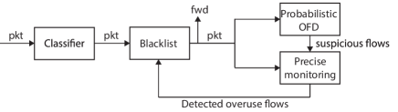
Figure 1: Router packet processing.

II-B Desired Properties

To ensure accurate and timely detection of overuse flows without affecting the regular packet processing, an overuse-flow detection algorithm should satisfy the following properties:

High-speed packet processing on routers

High-speed packet processing is required for a system that is deployed in the fast path of Internet routers (i.e., packet processing). However, high-speed memory that enables the necessary packet-processing frequency (e.g., SRAM) is expensive. Therefore, even core switches provide only a very limited amount of fast memory to ensure sustainable hardware cost. DRAM, albeit cheaper, is too slow to be accessed for every packet, but may be used for router slow-path operations (i.e., back-end processing on a CPU) without impacting fast-path forwarding. Moreover, even when accessing only SRAM in the router fast path, memory accesses should be employed economically to keep up with line rate.

Low false-positive and low false-negative rates

In the context of overuse flow detection, a false fositive (FP) is a misclassification of a non-overuse flow as an overuse flow. Conversely, a false negative (FN) is a misclassification of an overuse flow as a non-overuse flow, i.e., the failure of detecting an overuse flow. Although the precise-monitoring component of a flow-policing mechanism can prevent non-overuse flows from being falsely blacklisted, the detector itself should still ensure a low FP rate to not evict suspicious flows in the precise-monitoring component, thus increasing FN rates.

Detection of low-rate overuse flows

Overuse flows that are sending slightly above their permitted sending rate should be detected with high probability after a short amount of time. Our goal is to detect flows within at most seconds that are sending at $1.5$ their permitted rate; current state-of-the art algorithms typically assume $101000$ fold sending rates of overuse flows when budgeting resources.

II-C Overuse Flows vs. Large Flows

This work aims to efficiently detect overuse flows, and is inspired by algorithms for detecting large flows, i.e., flows which use a significant fraction of the link bandwidth.

However, it is important to note the significant differences between the two problems. In our context, large flows correspond to high-rate overuse flows, i.e., flows sending at rates at least $101000$ times higher than the average flow (for example, flows violating TCP fairness). The goal of previous work is to quickly identify the large flows to throttle or block them, thus preventing them from harming the other flows. These algorithms have a (more or less explicit) threshold above which a flow is considered large, but below which flows are allowed to send. This threshold is usually up to three orders of magnitude larger than the average flow’s sending rate—so a few flows sending around the threshold rate would rapidly exhaust link capacity and lead to congestion.

In the rest of this section, we briefly introduce two kinds of large-flow detection algorithms, namely sketch-based approaches and selective individual-flow monitoring. In the following, we discuss why they are inadequate for solving overuse-flow detection in our target scenario.

II-C1 Sketches

Individual-flow monitoring tracks the size of flows with a counter per flow, i.e., a memory cell that is increased by the packet size every time a packet of the corresponding flow arrives. To monitor flows using limited fast memory, sketches use each counter to track multiple flows. Two algorithms in this category are the Count-Min (CM) Sketch [13] (also known as Multistage Filters [16]) and Adaptive Multistage Filters (AMF) [14]. They rely on a relatively simple concept, which we illustrate at the example of the CM Sketch.

In the CM Sketch, flows are randomly mapped to counters, and each counter aggregates the volume of all flows that are assigned to it. If a large flow is mapped to a certain counter, this counter value is expected to be higher than the other counters as it includes the contribution of the large flow. To increase precision, the CM Sketch uses multiple stages, i.e., multiple counter arrays, and for each stage the flows are mapped to counters in a different way (e.g., using different hash functions). The CM Sketch classifies a flow as large if and only if the minimum value of counters to which the flow is mapped exceeds a certain threshold. For non-large flows, the probability that all associated counters exceed the threshold is low, decreasing exponentially in the number of stages.

However, achieving high accuracy with a CM Sketch is only possible with an untenable amount of memory. According to the theoretical work on the CM Sketch [13], the measurement error of the CM Sketch can be related to the amount of available memory. Concretely, a CM Sketch with $\lceil\ln(1/\delta)\rceil$ stages, each with $\lceil e/\epsilon\rceil$ counters, guarantees a probability of less than $\delta$ that the overestimation error amounts to more than a share $\epsilon$ of total traffic. Assuming that a switch with an aggregate bandwidth of $1\text{\,}\mathrm{Tbps}\text{/}$ handles $10$ millon flows [9] and that the overestimation should almost never exceed $50$% of the average-flow size (hence, $\delta=0.01$ and $\epsilon=0.5/10^{-7}$), then the CM Sketch would require around $250$ million counters. This memory consumption is even higher than allocating a counter per flow, which demonstrates that the CM Sketch is inaccurate on high-capacity routers.

Moreover, conventional sketches have been shown to be too inefficient to keep up with usual line speeds [22]. In order to achieve line rate, accuracy has to be traded for speed, which exacerbates the estimation error of sketches. In this work, we attempt to refine the sketch-based approach in order to achieve high accuracy with low processing complexity.

II-C2 Selective Individual-Flow Monitoring

Another category of large-flow detection algorithms dynamically selects a subset of flows for individual-flow monitoring. In the following section, we will illustrate the general idea of these schemes using the example of EARDet [38], which is one specimen of this category. Other examples include HashPipe [33] and HeavyKeeper [40].

EARDet is based on the Misra–Gries (MG) algorithm [25], which finds the exact set of frequent items (i.e., items making up more than a $1/k$-share of the stream) in two passes with limited counters. At a high level, the MG algorithm uses an array of counters to track frequent item candidates. By adjusting the counter values and associated items, the MG algorithm guarantees that every frequent item will occupy one counter after the first pass. The second pass is nevertheless required to remove falsely included infrequent items.

For each item in the stream, the MG algorithm adjusts the counters as follows. It first checks whether the item has occupied a counter in the array. If so, the corresponding counter will be increased by one. Else, if there is a non-occupied counter, the MG algorithm will assign that non-occupied counter to track this item (and also increase it by one). Otherwise, it will decrease all counters by one. The intuition is that infrequent items, should they be assigned to a counter, are likely to be evicted (i.e., their counter becomes zero) very quickly. By contrast, frequent items (which are already more likely to be assigned to a counter to begin with) are guaranteed to remain assigned to that counter, since their frequency compensates the occasional counter decreases.

EARDet enhances the MG algorithm to identify large network flows in one pass. EARDet is based on two flow specifications of the form $\gamma t+\beta$, where $\gamma$ is the allowed rate and $\beta$ is the allowed burst size. The adaptations guarantee that a flow sending less traffic than $\gamma_{l}t+\beta_{l}$ during any time window with length $t$ will not be falsely blocked (no false positive), and all large flows sending more than $\gamma_{h}t+\beta_{h}$ in any time window with duration $t$ will be caught (no false negative).

To catch overuse flows, EARDet could be configured to have $\gamma_{h}t+\beta_{h}$ set to the permitted bandwidth. However, given a low permitted bandwidth, this approach either demands many counters or suffers from high false negatives, as EARDet recommends using at least $\frac{\mathit{linkBW}}{\gamma_{h}}-1$ counters to achieve guaranteed detection. If $\gamma_{h}$ equals the maximum size of a non-overuse flow, fast memory would need to accommodate almost a counter per flow, which is infeasible on routers that handle millions of flows (cf. §II-A).

In addition to their high fast-memory consumption, the overhead of selective individual-flow monitoring, i.e., continuously deciding which flows to monitor closely, is prohibitively expensive in terms of processing complexity, which results in an insufficient throughput of such schemes (cf. §IV-H).

III LOFT Algorithm

LOFT is a novel design approach for a probabilistic overuse flow detector (OFD), the core component of a flow policing model in router packet processing. We first provide an overview of LOFT (§III-A) before describing the design in more detail (§III-B–III-D). We also provide a complexity analysis of the algorithm (§III-E).

TABLE I: Notation used in this paper.

Symbol	Description
$N$	Number of flows
$\gamma$, $\beta$	Rate and burst threshold flow specification
$\ell$	Overuse ratio
$\theta$	Number of minor cycles since last reset
$\omega$	Number of minor cycles per second
$Z$	Number of minor cycles per major cycle
$\theta_{reset}$	Reset cycle
$\lambda$	Sample rate
$W$	Number of counters in fast memory
$W_{\mathit{fm}}$	Number of precisely monitored flows
$U$	Flow-size estimate
$A$	Accumulated flow size
$C$	Accumulated flow count

III-A Overview

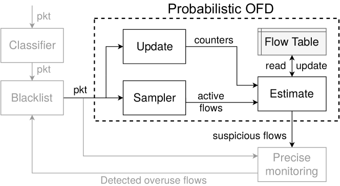
Figure 2: Details of the structure and information flow of the LOFT Probabilistic OFD component (cf. also Figure 1).

In this section, we describe our design for the probabilistic OFD component depicted in Figure 1. As Figure 2 shows, LOFT OFD contains four components: the update algorithm, the estimate algorithm, the sampler, and the flow table. Packets not rejected by the blacklist are forwarded to the update algorithm and the sampler. The estimate algorithm consumes their output, updates the flow table and creates a list of suspicious flows for precise monitoring.

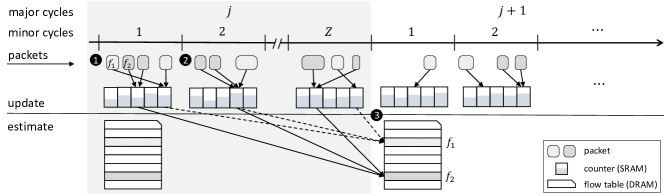
Figure 3: LOFT Timeline. ❶ A hash value is computed on the flow ID of the incoming packet, and the corresponding counter is increased by the packet size. ❷ A different set of counters and hash function are used when the minor cycle changes. ❸ After $Z$ minor cycles, the estimate algorithm aggregates the counter values and tries to identify a group of overuse flows.

The LOFT update algorithm targets one short time interval (e.g., $12.5\text{\,}\mathrm{ms}\text{/}$) at a time, which we call minor cycles. For each minor cycle, the update algorithm collects aggregated traffic information over groups of flows by using a single counter array. For every packet, LOFT maps the packet flow ID to one counter in the current counter array and increases that counter by the packet size. At the end of the minor cycle, the counter array is passed to the estimate algorithm.

The estimate algorithm operates on a larger time scale, at intervals (e.g., with duration $250\text{\,}\mathrm{ms}\text{/}$) that we call major cycles (see Figure 3): every time a major cycle is concluded, the estimate algorithm analyzes the counter arrays stored from all minor cycles during the major cycle, extracts estimates for the bandwidth utilization of every flow, and stores the estimates in a flow table. From this, the algorithm produces a list of suspected overuse flows, which is handed to the precise-monitoring component. The sampler provides a list of active flows which the estimate algorithm uses in its analysis.

In summary, the estimate algorithm uses the the sequence of counter arrays generated by the update algorithm to create a final flow estimate in each major cycle. Figure 3 visualizes how these algorithm components interact. By depicting packets of two different flows, the figure shows how flows are mapped to different counters in each minor cycle. Based on a packet’s flow ID, the update algorithm increases the associated counter by the packet size. Every major cycle, the estimate algorithm first updates the flow table based on the counter arrays generated in the most recent $Z$ minor cycles, recomputes the estimate for every active flow, and creates a watchlist from the $W_{\mathit{fm}}$ largest flows. The flows on the watchlist undergo precise monitoring in the subsequent major cycle. This precise monitoring is performed by the leaky-bucket algorithm [36], which detects any violation of a flow specification in form of $\gamma t+\beta$ (cf. §II) without false positives. Any flow that is found misbehaving by precise monitoring can thus be blocked by inserting it into the blacklist.

In the following, we will explain the design of the update algorithm (§III-B), the estimate algorithm (§III-C), and the sampler (§III-D). The pseudo code of the whole system is presented in Algorithm 1. The relevant notation is presented in Table I.

III-B Update Algorithm

Similar to a sketch, the LOFT update algorithm maps each flow to one counter in a counter array. Each counter tracks the aggregate bandwidth of all the flows mapped to that counter during a minor cycle. In each minor cycle, the association of flows to counters is randomized by changing the hash function for every minor cycle. When a minor cycle ends, the counter array is moved to main memory and an empty counter array is initialized in fast memory.

More formally, let $\mathit{ctr}_{j,k}$ be the counter array generated in the $k$-th minor cycle of major cycle $j$, and $H_{j,k}$ be the hash function used in that minor cycle. The value of $\mathit{ctr}_{j,k}[x]$ is the total packet sizes of flows that have been mapped to $x$ by $H_{j,k}$, i.e., all flows $f$ for which $H_{j,k}(f)=x$.

III-C Estimate Algorithm

At the end of a major cycle, which contains a certain number $Z$ of minor cycles, the estimate algorithm performs a flow-size estimation for every flow asynchronously (e.g., in user space of the router), while the update algorithm continues to aggregate traffic information. The flow-size estimate builds on two values: the volume sum and the cardinality sum.

For the volume sum, the estimate algorithm sums up the values of all the counters to which a flow was mapped. This aggregation over time reduces the counter noise in the sense of uneven flow size within the same counter: intuitively, an overuse flow, unlike a non-overuse flow, will be consistently associated with large counter values, which results in a large volume sum for that flow.

Although using multiple counters can reduce counter noise, it is neither sufficient nor innovative, as the Count-Min Sketch [13] uses the same idea (although by applying different hash functions concurrently instead of sequentially) and delivers insufficient performance. Indeed, the key to reducing counter noise lies in the cardinality sum. In order to compute this sum, an active-flow list is consulted to compute how many flows are associated with each counter within each minor cycle, i.e., the counter cardinality. For every flow, the estimate algorithm sums up the cardinality values of all counters associated with the flow. The cardinality sum reduces the distortion created by the varying cardinalities of counters: intuitively, an overuse flow will be associated with a large counter value even when the number of flows in that counter is small.

When dividing the volume sum by the cardinality sum, the strongest increases in a flow’s estimate are produced when the flow is mapped to high-value counters that contain a small number of flows. Indeed, flows with these characteristics are highly likely to be the largest flows among the investigated flows and are thus candidates for more precise monitoring.

Formally, after major cycle $j$, we define the estimate of a flow $f$ to be $\overline{U}_{f}^{(j)}=A_{f}^{(j)}/C_{f}^{(j)}$, where

$$A_{f}^{(j)} =\sum_{j^{\prime}\in J_{f}^{(j)}}\sum_{k=1}^{Z}\mathit{ctr}_{j^{\prime},k}[H_{j^{\prime},k}(f)]$$ (III.1a)

$$C_{f}^{(j)} =\sum_{j^{\prime}\in J_{f}^{(j)}}\sum_{k=1}^{Z}\left|\mathit{ctr}_{j^{\prime},k}[H_{j^{\prime},k}(f)]\right|$$ (III.1b)

where $J_{f}^{(j)}$ contains all major cycles $j^{\prime}\leq j$ in which flow $f$ was active. The term $|\mathit{ctr}_{j^{\prime},k}[x]|$ denotes the number of flows that have been mapped to counter $x$ in minor cycle $k$ of major cycle $j^{\prime}$ (counter cardinality). $A_{f}^{(j)}$ is the value aggregate of the counters that $f$ has been mapped to (volume sum) and $C_{f}^{(j)}$ is the summed count of the flows in these counters (cardinality sum). In order to avoid preserving counter arrays from past major cycles, the terms $A_{f}$ and $C_{f}$ are kept in the flow table and updated after every major cycle, i.e.,

$$\mathit{table}[f].A\leftarrow\mathit{table}[f].A+\sum_{k=1}^{Z}ctr_{j,k}[H_{j,k}(f)]$$ (III.2)

and analogously for $C_{f}^{(j)}$.These updates are made for all flows $f$ that were active in the most recent major cycle and are thus in the active-flow list generated by the sampler (cf. §III-D).

These estimates need to be adjusted when some flows send intermittently. For example, suppose flow $f_{1}$ sends $x$ $\mathrm{GB}\text{/}$ in the first and the third major cycle and nothing in the second major cycle, and flow $f_{2}$ sends $x$ $\mathrm{GB}\text{/}$ from the first to the third major cycle, i.e., $J_{1}^{(3)}=\{1,3\}$ and $J_{2}^{(3)}=\{1,2,3\}$. Then $A_{1}^{(3)}/C_{1}^{(3)}$ and $A_{2}^{(3)}/C_{2}^{(3)}$ will be almost the same. Suppose all counters contain exactly $y$ flows, then $A_{1}^{(3)}/C_{1}^{(3)}=\frac{x+x}{y+y}=\frac{x}{y}=\frac{x+x+x}{y+y+y}=A_{2}^{(3)}/C_{2}^{(3)}$. However, the total traffic sent by flow $f_{2}$ in these three cycles is actually 1.5 times larger than flow $f_{1}$ and should result in a higher flow-size estimate.

To fix this problem, we reduce a flow-size estimate $\overline{U}_{f}$ relative to the number of major cycles where flow $f$ was not active, i.e.,

$$U_{f}^{(j)}=\frac{|J_{f}^{(j)}|}{j}\cdot\frac{A_{f}^{(j)}}{C_{f}^{(j)}}$$ (III.3)

To enable this computation, the flow table must track $|J_{f}|$ for every flow $f$.

Another issue is that as $A_{f}$ and $C_{f}$ are accumulated, the estimate algorithm is actually computing their average over time. An attacker can take advantage of this approach by sending a low-rate traffic in the beginning for a period of time, and then start sending bursty traffic. It may not be detected by our system as its long-term average looks the same as a non-overuse flow, so old values must be discarded at some point. Therefore, we define the reset cycle $\theta_{reset}$, and clear all the data every $\theta_{reset}$ minor cycles. This reset may sound risky, as an overuse flow could send its traffic around the reset point so that its estimated size is reset before being detected by our system. However, an attacker does not know the reset point. Moreover, even if an attacker could infer the reset point, the overuse traffic sent by a flow with such a strategy is bounded, as we show in the mathematical analysis (Appendix A).

III-D Sampler

Clearly, LOFT requires a list of active flows for which an estimate must be computed. In order to generate such an active-flow list, we use sampling and limit the number of sampled packets per second to be $\lambda$. LOFT considers a randomized sampling period, which is a random variable of an exponential distribution with mean $\frac{1}{\lambda}$. This randomization prohibits an attacker flow from circumventing the sampling by sending at the appropriate moments.

Having an active-flow list for a major cycle $j$ also allows to compute the cardinality $|\mathit{ctr}_{j,k}[x]|$ of counters in the estimate algorithm, namely by counting how many active flows were mapped to each counter with the respective hash function $H_{j,k}$ for any minor cycle $k$. An alternative to this reconstruction of counter cardinality would consist in measuring counter cardinality within the update algorithm, for example using a Bloom filter [8] or HyperLogLog register [17] per counter. However, as fast memory is the bottleneck resource, additional computational complexity in the estimate algorithm is preferable to estimating cardinality in fast memory.

Algorithm 1 LOFT algorithm.

1:procedure Process($pkt$)

2:    if $pkt.flowID\in blacklist$ then

3:         return     

4:    if $pkt.flowID\in watchlist$ then

5:         Monitor($pkt$)     

6:    $j\leftarrow$ GetMajorCycle()

7:    $k\leftarrow$ GetMinorCycle()

8:    Sampler($pkt$)

9:    Update($pkt$, $j$, $k$)

10:    if $Z\cdot j\geq\theta_{reset}$ then

11:         Reset()     

12:procedure Sampler($pkt$)

13:    if $\mathit{current\_time}\geq\mathit{sample\_time}$ then

14:         $activeFlow\leftarrow activeFlow\cup\{pkt.flowID\}$

15:         $u$ samples uniformly from $\mathcal{U}(0,1]$

16:         $sample\_time\leftarrow sample\_time-\frac{\ln{u}}{\lambda}$     

17:procedure Update($pkt$, $j$, $k$)

18:    $x\leftarrow H_{j,k}(pkt.flowID)$

19:    $\mathit{ctr}_{j,k}[x]\leftarrow ctr_{j,k}[x]+pkt.size$

20:procedure Estimate()

21:    $j\leftarrow$ GetMajorCycle() - 1

22:    for $k=1$ to $Z$ do

23:         for $f\in activeFlow$ do

24:             $x\leftarrow H_{j,k}(f)$

25:             $numFlow[x]\leftarrow numFlow[x]+1$          

26:         for $f\in activeFlow$ do

27:             $x\leftarrow H_{j,k}(f)$

28:             $A[f]\leftarrow A[f]+ctr_{j,k}[x]$

29:             $C[f]\leftarrow C[f]+numFlow[x]$              

30:    $N\leftarrow|activeFlow|$

31:    for $f\in activeFlow$ do

32:         $table[f].A\leftarrow table[f].A+A[f]$

33:         $table[f].C\leftarrow table[f].C+C[f]$

34:         $table[f].\mathit{numJ}\leftarrow table[f].\mathit{numJ}+1$     

35:    $activeFlow\leftarrow\emptyset$

36:    return $W_{\mathit{fm}}$ flows with largest $\frac{table[f].\mathit{numJ}}{j}\cdot\frac{table[f].A}{table[f].C}$

III-E Complexity Analysis

In summary, the update algorithm uses $O(W)$ fast-memory entries, where $W$ is the width of a counter array. The number of read and write operations is linear in the number of packets. The estimate algorithm uses $O(ZW+N)$ entries in DRAM, and the number of accesses is $O(ZN)$.

III-E1 Time complexity

In the update algorithm, each packet requires a single read and a single write operation to fast memory. Moreover, the algorithm requires a single hash function computation, which results in the major advantage that LOFT achieves line rate (see §IV-H), whereas other sketch-based algorithms update multiple counter arrays per packet and therefore fall short of that goal [22]. The hash computation itself can be performed in hardware or using an efficient software implementation such as the murmur3 hash function.

The estimate algorithm uses multiple accesses to main memory. However, the number of accesses is linear in the number of active flows, which may be much smaller than the number of packets. In each major cycle, we need to sum up the corresponding counters in each minor cycle for each flow. Suppose there are $N$ active flows, then there are $O(ZN)$ DRAM reads to compute the updates to the estimate components. After obtaining these values, we need to update the flow table. For each active flow, the algorithm performs one lookup and update to the hash table. We use a Cuckoo hash table [27], which has worst-case constant lookup time. Although the worst-case insertion time of the Cuckoo table might be long, its expected complexity is amortized constant. Additionally, the number of insertions is much lower than the number of lookups as each flow will be inserted only once when it’s first seen. Therefore, the update takes $O(N)$ time.

In the sampler, for every sampled packet, there is one insertion to the active-flow list stored in DRAM, for which we again used a Cuckoo hash table. By properly setting the table capacity and sample rate $\lambda$, our experiments show that the sampler is still fast enough to keep up with line speeds.

III-E2 Space Complexity

Only counters of the current minor cycle reside in fast memory, which is $O(W)$ and depends on the size of a counter. Our analysis shows that, if all flows send almost at threshold rate, a small $W$ (e.g., $8192$) can lead to considerable detection delay.

Other counters are kept in main memory before being handled by the estimate algorithm, which takes $O(ZW)$ space. The active-flow list and the flow table are also in DRAM. The active-flow list requires $O(N)$ entries and the space complexity of the flow table is also linear to $N$ (using a Cuckoo table). Therefore, the total number of main memory entries used (including counters) is $O(ZW+N)$.

IV Evaluation

The evaluation of LOFT is conducted through two implementations and a simulation. First, the behavior of LOFT in a real-world environment is evaluated using the implementations and a testbed that supports up to 4x$40\text{\,}\mathrm{Gbps}\text{/}$ traffic volume. Second, to evaluate the accuracy of LOFT and compare it to EARDet, AMF, HeavyKeeper and HashPipe, simulations with a traffic volume equivalent to 4x$100\text{\,}\mathrm{Gbps}\text{/}$ are used.

IV-A Implementation

For the scalability experiments with DPDK, we implemented LOFT in C on the Intel DPDK framework [28]. The application uses $n$ worker threads that execute the update algorithm and a separate thread running the estimation algorithm every major cycle. The major and minor cycle indices are computed based on a monotonic clock with nanosecond resolution.

For further scalability experiments, we also implemented the update algorithm of LOFT on a Xilinx Virtex UltraScale+ FPGA on the Netcope NFB 200G2QL platform [2] containing two $100\text{\,}\mathrm{Gbps}\text{/}$ NICs. Presenting the detailed contributions of the FPGA implementation would exceed the scope of this paper. Therefore, a separate paper illustrating the design of the FPGA implementation has been submitted to a specialized conference [4].

In order to test the accuracy of LOFT, we evaluated LOFT and other algithms in simulations using Rust (LOFT, EARDet, AMF) and Golang (HeavyKeeper, HashPipe).

IV-B Experiment Setup

Test Setup

The testbed for the DPDK scalability experiment consists of two machines connected using 4x$40\text{\,}\mathrm{Gbps}\text{/}$ Ethernet connections. The traffic is generated using a dedicated traffic generator (Spirent TestCenter N4U [34]) and sent to a commodity machine with an Intel Xeon E5-2680 CPU. For the simulations, we execute LOFT on an Intel Xeon 8124M machine and process synthesized traffic equivalent to 4x$100\text{\,}\mathrm{Gbps}\text{/}$.

Traffic Generation

To evaluate the scalability of LOFT with respect to flow volumes, we generated network traces with uniform packet sizes and based on an iMix traffic distribution (avg. size: $353\text{\,}\mathrm{B}\text{/}$) [26].

IV-C Evaluation Metric: Detection Delay

The detection delay of an overuse flow is the time elapsed between the first violation of the flow specification and the time the flow is caught by a detector. A detection delay longer than the simulation timeout results in a false negative.

When presenting detection rates and false negatives, it is always crucial to present the corresponding false positive rate, i.e., the number of non-overuse flows incorrectly marked as malicious. We note, however, that LOFT is designed to have no false positives, because benign flows that happen to be flagged as suspicious by the estimation algorithm will be exonerated by precise monitoring.

IV-D Parameter Selection

Several of LOFT’s parameters can be tuned to fit the hardware restrictions of a specific deployment. In the following, we describe how to experimentally determine these parameters so that they comply with the hardware’s computational constraints even under the worst-case traffic patterns.

To experimentally determine the sampling rate, we increase the sampling rate of the sampler until its CPU core is fully utilized, such that the accuracy of the flow ID list is maximized. With this determined sampling rate and an estimated maximum number of flows, we calculate the maximum number of major cycles per second such that there are enough samples between two executions of the estimation algorithm to build the flow ID list with the desired accuracy. Finally, we increase the number of minor cycles per second until the CPU core of the estimation algorithm is fully utilized. Table II summarizes these hardware-related parameters used in our experiments.

The flow monitor is set to monitor 64 flows simultaneously in all experiments, which is small and fast enough to keep up with a high-bandwidth link. Finally, with the determined parameters in Table II, the reset cycle parameter $\theta_{reset}$ in each experiment is adjusted to achieve $95$% detection probability (detailed in the mathematical analysis in Appendix A) under the given experiment setting.

TABLE II: Hardware-related LOFT parameters.

Parameter	Value
Sampling rate ($\lambda$)	$2.1\cdot 10^{6}$ samp./s
Number of minor cycles	$64$ cycles/s
Number of major cycles	$14$ cycles/s

IV-E Comparison: Fully Utilized Traffic Trace

We first evaluate LOFT in a setting where every flow sends at a rate close to the maximum allowed threshold, fully utilizing the reserved bandwidth.

We simulate a configuration with 4x$100\text{\,}\mathrm{Gbps}\text{/}$ links with an aggregate number of $130^{\prime}000$ flows, where each flow requires $3\text{\,}\mathrm{Mbps}\text{/}$, e.g., for high-quality video streaming. Then, a misbehaving flow with an overuse ratio $\ell$ is injected. Each detector allocates $16^{\prime}448$ counters in fast memory. LOFT, AMF, HashPipe and HeavyKeeper use $64$ counters (out of $16^{\prime}448$) as flow monitors. To optimize detector performance for AMF, HashPipe and HeavyKeeper, the fast-memory counters are structured as counter arrays. LOFT is configured to run $4$ cycles of the estimation algorithm per second, which reaches the computation limit on our machine.

Figure 4(a) shows the detection delays of LOFT, EARDet, HashPipe, HeavyKeeper and AMF under different overuse ratios $\ell$ on a log-log scale. Each data point is averaged over $100$ runs. We find that LOFT detects a $1.5$x overuse flow in less than one second, whereas all other detectors fail to detect it before the $300\text{\,}\mathrm{s}\text{/}$ timeout. For larger overuse flows, LOFT still outperforms AMF, EARDet, HashPipe and HeavyKeeper when the overuse ratio is less than $400$x, $7$x and $3$x, respectively. As opposed to HashPipe and HeavyKeeper, LOFT delivers high accuracy at a lower variance. Moreover, LOFT can achieve much higher throughput (cf. §IV-H).

The reason that LOFT is slower in detecting high-rate overuse flows is that it needs at least one major cycle, which takes $0.25\text{\,}\mathrm{s}\text{/}$, to select the overuse flow. These results confirm that LOFT can efficiently detect overuse flows using a small amount of router resources. While heavy-hitter detection schemes perform better than LOFT regarding the extremely large flows that they are designed to catch, these schemes are ineffective in low-rate overuse flow detection, which is the goal of this paper.

As Figure 4(b) shows, these results are confirmed by performing the same experiments with $10$ million flows, which is the number of flows to be expected on a $\mathrm{Tbps}\text{/}$ link (cf. Section II-A). For $10$ million flows, the higher accuracy of LOFT is even more prominent, as even the best other schemes (i.e., HashPipe and HeavyKeeper) fail to detect the overuse flows for all overuse ratios below $20$.

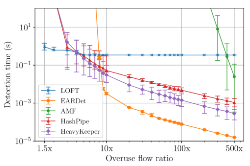
(a) $N=130K$

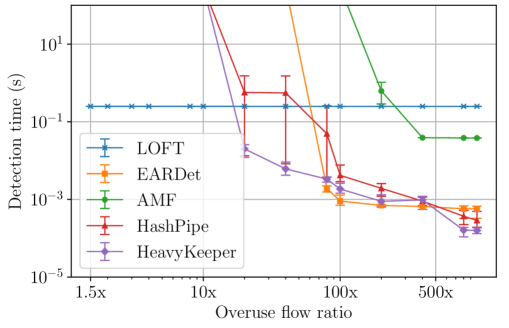
(b) $N=10M$

Figure 4: Detection delay of overuse flow detectors under different overuse ratios and flow numbers $N$. The error bars show the minimum and maximum values over 100 runs.

IV-F Comparison: CAIDA Traffic Trace

In addition to using synthesized background traffic in which every non-overuse flow fully utilizes the reserved bandwidth, we also compare detectors on an OC192 link using a real traffic trace, namely the CAIDA New York Anonymized Internet Trace [9]. In the trace, the majority of the flows are smaller than $512$ bytes per second, and $95$% of the flows are smaller than $14^{\prime}000$ bytes per second.

We first regulate every flow in the CAIDA trace with the permitted bandwidth $\gamma$. Flows that use more than the permitted bandwidth are governed by dropping overuse packets. Then, a 2-fold overuse flow is added into the traffic trace. This setting reflects the scenario where an ISP wants to mitigate DDoS by putting a bandwidth cap on individual flows. Because the number of flows in the CAIDA traffic is smaller than in the fully utilized traffic trace, on this smaller network, we only allocated $2048$ + $64$ counters to all detectors ($64$ flow monitors). LOFT is configured to run $4$ slices of the estimation algorithm per second.

Figure 5 shows the detection delays of LOFT, EARDet, AMF, HashPipe and HeavyKeeper under different permitted bandwidths on a log-log scale. Each data point is averaged over $100$ runs. LOFT detects the 2-fold overuse flow in $0.31.5\text{\,}\mathrm{s}\text{/}$. EARDet and AMF can quickly and reliably detect the 2-fold overuse flow only when it is much larger than the majority of the non-overuse flows. HashPipe and HeavyKeeper catch the overuse flow also given a low threshold, but these schemes still require a multiple of LOFT’s detection time to identify the overuse flow. Furthermore, the throughput of these schemes is substantially lower than the throughput of LOFT (cf. §IV-H).

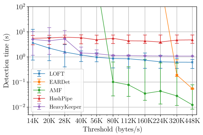
Figure 5: Detection time of overuse flow detectors to catch a overuse flow sending $2\gamma$ given CAIDA traffic with different regulation threshold $\gamma$ and $\beta=1500$ for all.

IV-G LOFT Sensitivity Tests

We have shown that given the same memory budget, LOFT can detect low-rate overuse flows much faster than AMF, EARDet, HashPipe and HeavyKeeper. The following experiments further investigate LOFT’s effectiveness by varying its parameters under a background traffic setting that is challenging for all evaluated detectors.

LOFT is configured to run one slice of the estimation algorithm per second since it has to process more flows in the following tests. We consider a half-utilization scenario, in which a half of the non-overuse flows send up to the permitted bandwidth, and the rest sends almost negligible traffic. This is a more challenging scenario than full utilization for LOFT because the variance between counters are not only affected by the number of flows aggregated but also by the variance of flow sizes. This half-utilization scenario can capture the behavior of typical streaming traffic, in which one direction is used to send data and the other to send ACKs.

Half of the non-overuse flows send traffic up to the flow specification $\gamma=\frac{400Gbps}{N}$ and $\beta=1500$ and the other half send 25 times less traffic. As before, one overuse flow is injected in the simulation. This $\ell$-fold overuse flow follows a flow specification $\gamma=\frac{400Gbps}{N}\cdot\ell$ and $\beta=1500$. Each data point of detection delay is the average of 100 simulations.

Flow counting drastically reduces the detection time

Figure 6 shows that the estimator with flow counting and dividing significantly outperforms the one without counting. This result supports our perspective in Section III-A that the detection accuracy of sketches is suffered by not taking the number of flows into account. In other words, LOFT is highly accurate thanks to its efforts to reduce the counter noise that stems from the variance of counter cardinality.

Figure 6: LOFT’s detection time of an overuse flow with and w/o counting. $N=130K$, $W=16384$, $\ell=1.5$.

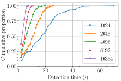
(a) $N=400K$, $r=0\%$, varying $W$

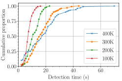
(b) $W=1024$, $r=0\%$, varying $N$

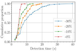
(c) $N=400K$, $W=16,384$, varying $r$.

Figure 7: CDF of LOFT’s detection delay given number of counters ($W$), number of flows ($N$), and sampling miss rate ($r$).

Memory budget

In this experiment, we investigate the impact of fast memory size on the detection delay. Figure 7(a) shows the cumulative distribution of the detection delay given different numbers of fast-memory counters, ranging from $1024$ to $16^{\prime}384$. As the number of fast-memory counters is doubled, LOFT’s detection speed increases as lowering the number of flows sharing a counter reduces the variance of each counter. However, even with the maximum number of counters and including the memory required for monitoring suspicious flows, the fast-memory consumption of LOFT is around $130\text{\,}\mathrm{kB}\text{/}$, which represents more than an order of magnitude reduction compared to the $3\text{\,}\mathrm{MB}\text{/}$ of fast memory needed for individual-flow monitoring under the same traffic conditions (cf. §II-A).

Number of non-overuse flows

We evaluate the impact of the number of non-overuse flows on the detection delay. Using $1024$ fast-memory counters and one 2-fold overuse flow, Figure 7(b) shows the cumulative detection delay given different numbers of non-overuse flows, ranging from $100^{\prime}000$ to $400^{\prime}000$. The detection delay grows with the number of non-overuse flows because the variance of counter cardinality increases as the total number of flows grows.

Imprecise active-flow list

In our previous experiments, the fixed sampling rate (as defined in Table II) is sufficient to maintain a precise active-flow list. Given that maintaining this list is bound by the hardware-limited sampling rate, the number of active flows might be too high to build a precise active-flow list. For example, for $400^{\prime}000$ active flows and a sampling rate of $800^{\prime}000$ flows per major cycle, the active-flow list will miss about $15$% of active flows.

To understand the impact of an imprecise active flows list on LOFT, we evaluate different miss rates of active-flow lists. Figure 7(c) shows that in case of the half-utilization scenario, LOFT performs worse with increasing imprecision of the active-flow list. This is due to the reason that LOFT will use an inaccurate number of flows to calculate estimators, which leads to higher variance. Nevertheless, even missing $20$% of active flows, LOFT can still catch the overuse flow under $14\text{\,}\mathrm{s}\text{/}$ with $95$% probability.

IV-H Scalability of LOFT

IV-H1 DPDK Implementation

To understand the scalability of LOFT in a DPDK environment, we evaluate the maximum packet rate with respect to the packet size and number of cores that execute the update algorithm concurrently. Figure 8(a) shows that LOFT is able to achieve line-rate for iMix-distributed traffic using $16$ cores that execute the update algorithm and one core that runs the estimation algorithm. For smaller numbers of cores, line-rate can only be achieved for larger packet sizes ($1024\text{\,}\mathrm{B}\text{/}$).

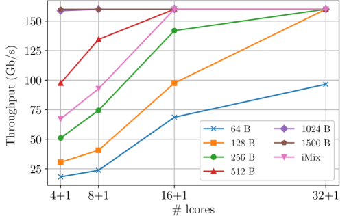
(a) Throughput given number of logical cores and packet sizes.

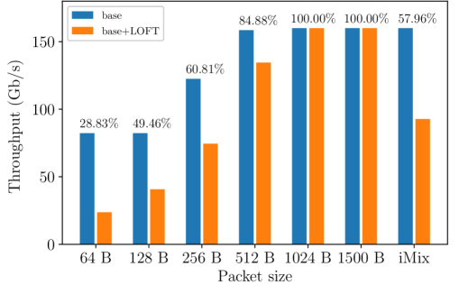
(b) Overhead compared to regular L3 forwarding for 8+1 cores.

Figure 8: DPDK implementation results.

Since traffic flows with small sized packets perform considerably worse than flows with large packet sizes, we additionally evaluate the overhead introduced by LOFT by comparing it to regular L3 packet forwarding in DPDK. Figure 8(b) shows the throughput of regular L3 forwarding and the throughput of forwarding with additional LOFT processing for different packet sizes. Moreover, the figure gives the LOFT throughput as a percentage of the corresponding base throughput. As visible in the figure, even regular L3 packet forwarding using eight processing cores cannot achieve line-rate for packet sizes smaller than $1024\text{\,}\mathrm{B}\text{/}$. Compared to regular packet forwarding, LOFT introduces overhead for small packet sizes, which results in a maximum packet rate of ~$50$ million packets per second ($\mathrm{Mpps}\text{/}$) using eight processing cores, i.e., ~$6\text{\,}\mathrm{Mpps}\text{/}$ per core. As for larger packet sizes this maximum packet rate does not get exhausted, this effect is diminished. However, LOFT still achieves a much higher packet rate than the alternative schemes with the best accuracy, i.e., HashPipe and HeavyKeeper: Prior work has shown a packet rate of ~$2\text{\,}\mathrm{Mpps}\text{/}$ per core for HashPipe [39] and a packet rate of ~$2.5\text{\,}\mathrm{Mpps}\text{/}$ per core for HeavyKeeper [40].

IV-H2 FPGA Implementation

We also implemented the fast-path component of LOFT (i.e., the update algorithm using $16^{\prime}384$ counters) on a Xilinx Virtex UltraScale+ FPGA on the Netcope NFB 200G2QL platform [2] with two $100\text{\,}\mathrm{Gbps}\text{/}$ NICs and an operating frequency of $200\text{\,}\mathrm{MHz}\text{/}$. The LOFT implementation can process a packet in every cycle. For minimum-size packets of $64\text{\,}\mathrm{B}\text{/}$, each NIC manages to transfer one packet per cycle to the LOFT implementation, which allows to achieve a packet rate of $200\text{\,}\mathrm{Mpps}\text{/}$ per NIC. As the FPGA platform contains two NICs, it achieves a total packet rate of ~$400\text{\,}\mathrm{Mpps}\text{/}$. This high throughput demonstrates that LOFT is suitable for high-speed packet processing if implemented on programmable NICs. The full implementation is described in a paper submitted to a specialized conference [4], as the FPGA-specific implementation details represent a contribution that goes beyond the scope of this paper.

V Theoretical Analysis Results

In the mathematical analysis provided in Appendix A, we analyze the overuse flow detection, and derive a lower bound (Equation A.15) for the probability that an overuse flow is detected within a reset cycle, i.e., before a reset. This bound depends on a number of parameters of LOFT. The most important are the duration of a reset cycle $T_{\mathit{reset}}$ (where $T_{\mathit{reset}}\triangleq\omega^{-1}\theta_{reset}$) and the number of fast-memory counters $W$.

By requiring that the lower bound be equal to a desired detection probability, we compute an upper bound on the required duration $T_{\mathit{reset}}$ of a reset cycle for a given number of counters in order to achieve that detection probability.

Table III shows the reset cycle duration $T_{\mathit{reset}}$ calculated under the settings from the experiment of Figure 7(a), compared to the real detection delays as obtained by our analysis in Section IV-G. The result shows that our analysis does not underestimate the detection delay, since the upper bound on the reset cycle duration, which is the worst-case-estimate of the 95th percentile of the detection delay, is always higher than those obtained by our evaluation. The reasons why the estimated delay is $25$ higher than the real one are twofold. First, the synthesized traffic in our experiments does not always represent the worst-case scenario. Second, LOFT ranks and detects overuse flows at the end of every estimation algorithm, but our analysis ignores the probability that overuse flows might be caught at some point before $\theta_{reset}$, which loosens the bound.

TABLE III: Calculated reset cycle duration ($T_{\mathit{reset}}$) and the real 95th percentile of the detection delay from our evaluation with different numbers of counters in fast memory in the experiment of Figure 7(a).

Num. of counters	$1024$	$2048$	$4096$	$8192$	$16^{\prime}384$
Reset cycle ($\mathrm{s}\text{/}$)	$231$	$116$	$58$	$29$	$15$
Detection delay ($\mathrm{s}\text{/}$)	$43.03$	$20.48$	$14.04$	$8.67$	$6.52$

VI Related Work

Despite a significant amount of research on the problem of detecting high-rate overuse flows, the problem of efficiently detecting low-rate overuse flows has so far been neglected. A number of related schemes have been proposed to address similar problems, such as large flow detection and top-k flow detection. Their ideas might be applicable to detecting overuse flows. However, we discuss in the following paragraphs that they are either orthogonal to our research direction, or that they are insufficient to solve our problem as stated in Section II.

The problem of detecting top-k flows aims to identify $k$ flows that consume most of a link’s bandwidth. A recent proposal called HashPipe [33] tackles the heavy hitter detection problem on programmable hardware. To ensure line-rate detection given a limited amount of fast memory, HashPipe constructs a pipeline of hash tables to efficiently implement the Space Saving algorithm [24], such that the heavier flows are more likely to be kept in the next stage of the pipeline. However, our results in §IV show that HashPipe fails to detect the overusing flow in cases where the difference between overuse and non-overuse flow is low (i.e., with an overuse ratio of $1.52$). As another top-k detection scheme, HeavyKeeper [40], seems to suffer from the same weakness, these systems seem unable to effectively filter out the counter noise.

Similar to top-k flow detection, large-flow detection algorithms can be applied to detecting overuse flows. Large flow detection algorithms identify flows that use more than a threshold amount of bandwidth, and it is common that the higher the threshold the better the performance will be. Besides AMF (introduced in Section II-C), CLEF [37] proposes to detect low-rate overuse flows, which are similar to the low-rate overuse flows in our work, using recursive division and by combining two detectors with complementing properties. Our evaluation shows that LOFT outperforms EARDet, one of the detectors used by CLEF, when the overuse ratio is lower than $7$x. The other detector used by CLEF is a sketch and thus inherits the limitations explained in Section II-C.

Hybrid SRAM/DRAM-based architectures for exact counting have been proposed by Shah et al. [32] and were further improved by Ramabhadran and Varghese [29] and by Zhao et al. [41]. By default, these schemes only consider the number of packets per flow, but not the flow sizes. Even though the authors propose an extension to consider flow sizes, the use of probabilistic counting in these schemes introduces a high counter variance, making low-rate overuse flows hard to detect. Lall et al. [21] propose another SRAM/DRAM hybrid data structure for efficient detection of both medium and large flows. However, because the proposed flow monitoring solution uses shared counters (in the form of spectral Bloom filters), it performs poorly in catching low-rate overuse flows.

Another approach to tackle aforementioned problems uses sampling, where only a small subset of packets is used for flow accounting. Sampled NetFlow [12] is a widely deployed solution that collects one out of every $n$ packets, and estimates statistics of the original population by extrapolating from the sample. Researchers have proposed advanced sampling algorithms tailored for catching large flows. For example, Sample and Hold [16] and Sticky Sampling [23] are designed to bias toward large flows. Instead of using a static sampling rate, several adaptive sampling algorithms dynamically adjust the sampling rate so as to keep resource consumption under a fixed memory limitation [15, 31]. However, without a sufficiently high sampling rate (resulting in a large amount of fast memory), sampling-based algorithms are prone to false positives and false negatives, as shown by Estan and Varghese [16]. LOFT relies on sampling to generate a list of active flows (if the list is not provided). However, LOFT ensures that at least one packet appears in a sample, thus requiring a lower sampling rate than for accurate flow accounting.

A recent series of work including SketchVisor [19], ElasticSketch [39] and NitroSketch [22] devises techniques to speed up the updating of detector datastructures based on sketches. However, these techniques all trade off detection accuracy against processing speed, i.e., these algorithms achieve even lower accuracy than the unaltered sketches like AMF evaluated in Section IV. In contrast, LOFT can achieve high accuracy and a low per-packet overhead.

VII Conclusions

Due to limitations of previous approaches to probabilistic flow monitoring, network operators so far lacked effective measurement tools that could give an accurate insight into the flow-size distribution on high-capacity routers. Given router constraints regarding fast memory and computation, existing schemes suffer from a large measurement error, which only allows the reliable detection of extremely large flows, but not flows with a small amount of overuse. In this work, we show that the source of this measurement error in sketch-based schemes is counter noise, i.e., the high variance of counter values. Using this insight, we develop LOFT, a sketch-based approach that counteracts the counter noise while respecting the stringent complexity constraints of high-speed routers.

As a result, the measurement error of LOFT is so small that low-rate overuse flows (i.e., flows only $50100$% larger than the average flow) can be reliably detected with a small amount of fast memory. Concretely, LOFT can reliably identify a flow that is only $50$% larger than the average flow within one second, whereas all other investigated schemes fail to identify such a flow even within $300\text{\,}\mathrm{s}\text{/}$. Moreover, LOFT accomplishes such high accuracy while reducing the fast-memory requirement by more than one order of magnitude in comparison with individual-flow monitoring. We also investigate scalability and overhead of LOFT with a DPDK and an FPGA implementation, and show that LOFT enables line-rate forwarding of a realistic traffic mix.

With these demonstrated properties, LOFT can serve as a powerful flow-monitoring tool, which will allow network operators to improve the efficacy of existing applications based on flow-size estimation (e.g., flow-size aware routing) and to enable new applications based on such estimates (e.g., reservation-based DDoS defense).

Appendix A Mathematical Analysis

We would like to know the probability that LOFT can catch overuse flows and how much damage they can do before being caught. Our analysis first derives a lower bound on the probability that a non-overuse flow estimate becomes larger than an overuse flow estimate. Then we use this bound to calculate the probability that an overuse flow estimate falls within the top-$W_{\mathit{fm}}$ largest estimates, which is also the probability of being monitored.

Due to the complexity of this problem, we make the following assumptions throughout the analysis. We require that the number of flows $N$ in traffic is fixed during each detection period and $N$ is large enough so that the attacker is unable to manipulate either $N$ or the overall traffic size distribution. In addition, we assume that all flow estimates, which are random variables in our model, only have weak pairwise dependence, and see them as i.i.d. in the following analysis.

A-A Lower Bound of Detection Probability

First we derive a lower bound of the dectection probability given the amount of an overuse flow after LOFT starts a reset cycle. This lower bound helps us analyze how long LOFT will need to catch the overuse flow with high enough probability. Then by setting a proper reset cycle, our analysis determines the maximum damage an overuse flow can do, and guarantees that LOFT will have high probability to catch the overuse flow if it exceeds the limit of maximum damage.

The detection probability of an overuse flow is exactly the probability of LOFT choosing to monitor that flow and the flow monitor catches its overusing behavior. Here we ignore the time spent in the flow monitor when an overuse flow is reported to it. Analyzing and improving flow monitor is outside the scope of this paper. Therefore, the detection probability is equal to the probability of the overuse flow being selected by LOFT.

We define $U_{i}$, $A_{i}$, $C_{i}$ as the estimate, accumulator, and counter of flow $i$ in our algorithm, respectively. Hence they have the following relationship:

$$U_{i}=\frac{A_{i}}{C_{i}}$$ (A.1)

In each minor cycle, each flow, except for flow $i$, has $\frac{1}{W}$ chance to contribute part of its flow size to $A_{i}$. We define a flow segment $X_{j}$ as the amount contributed by another flow $j$ to $A_{i}$ in a minor cycle. Every $X_{j}$ can be seen as a random variable with unknown distribution, since it is selected randomly by a uniform hash function. More deeply, suppose $S_{a}=\{X_{1},X_{2},\cdots,X_{a}\}$ and $S_{b}=\{X_{a+1},X_{a+2},\cdots,X_{a+b}\}$ are added to $A_{i}$ in minor cycle $x$ and $x+1$, respectively. $S_{a}$ are exactly the $a$ uniform samples without replacement from $N$ flow segments sent by $N$ flows during minor cycle $x$. In addition, $S_{b}$ are another $b$ uniform samples from minor cycle $x+1$ and being independent of the prior samples $S_{a}$, since $S_{a}$ and $S_{b}$ are sampled independently from two different sets of flow segments. These properties allow us to apply Hoeffding’s inequality [18] and derive the bound in Equation A.8.

Because we assume that overuse flows are minority and cannot affect the traffic distribution, and because all other flows will not violate the flow specification, $X_{j}$ also satisfies the following bound, where $M\triangleq\gamma\omega^{-1}+\beta$.

$$0\leq X_{j},E[X_{j}]\leq M$$ (A.2)

Suppose LOFT has run $\theta$ minor cycles, given there are $c_{i}$ flow segments accumulated in $C_{i}$, the size of flow $i$ is $F_{i}$, we can represent $U_{i}$ as a random variable under this condition as below.

$$U_{i}|(C_{i}=c_{i})=\frac{1}{c_{i}}(F_{i}+\sum_{j=1}^{c_{i}-\theta}X_{j})$$ (A.3)

From Equation A.3, now $U_{i}$ is modeled by the sum of several random variables, which is also a random variable with unknown distribution. As mentioned previously, different $U$s are seen as i.i.d. This assumption is reasonable because under random dispatching the probability that any pair of $U$ share many $X$ (and thus build strong dependence) is extremely low. The more precise analysis is left for future work.

Let $U_{l}$ and $U_{b}$ be the estimates of an overuse flow and a non-overuse flow respectively. By Equation A.3, we can enumerate all conditions and derive the equation below (In the following equations, we short $C_{i}=c_{i}$ to $\overline{c_{i}}$).

$$P(U_{l}>U_{b})=\sum_{c_{l}=1}^{N\theta}\sum_{c_{b}=1}^{N\theta}P(U_{l}>U_{b}|\overline{c_{l}},\overline{c_{b}})P(\overline{c_{l}},\overline{c_{b}})$$ (A.4)

Instead of bounding Equation A.4 directly, we choose a threshold $\tau$ and simplify the bound with the following inequality, which holds since $U_{l}$ and $U_{b}$ are i.i.d. in our assumption.

$$P(U_{l}>U_{b}|\overline{c_{l}},\overline{c_{b}})\geq P(U_{l}>\tau|\overline{c_{l}})P(U_{b}<\tau|\overline{c_{b}})$$ (A.5)

Combining with Equation A.4, we have the following inequality.

$$P(U_{l}>U_{b})\geq\sum_{c_{l}=1}^{N\theta}\sum_{c_{b}=1}^{N\theta}P(U_{l}>\tau|\overline{c_{l}})P(U_{b}<\tau|\overline{c_{b}})P(\overline{c_{l}},\overline{c_{b}})$$ (A.6)

Now the goal is deriving the bound of $P(U_{i}>\tau|\overline{c_{i}})$. Suppose $c_{b}-\theta\geq 1$, for the estimate of non-overuse flow $U_{b}$, combining with Equation A.3, we have the following inequality.

$$P (U_{b}\geq\tau|\overline{c_{b}})$$ (A.7)

$$=P(\frac{1}{c_{b}}(F_{b}+\sum_{j=1}^{c_{b}-\theta}X_{j})\geq\tau)$$

$$=P(\frac{1}{c_{b}}F_{b}+\frac{c_{b}-\theta}{c_{b}}\frac{1}{c_{b}-\theta}\sum_{j=1}^{c_{b}-\theta}X_{j}\geq\tau)$$

$$=P(\frac{1}{c_{b}-\theta}\sum_{j=1}^{c_{b}-\theta}X_{j}\geq\frac{c_{b}}{c_{b}-\theta}(\tau-\frac{F_{b}}{c_{b}}))$$

$$=P((\frac{1}{c_{b}-\theta}\sum_{j=1}^{c_{b}-\theta}X_{j})-E[X]\geq\frac{c_{b}}{c_{b}-\theta}(\tau-\frac{F_{b}}{c_{b}})-E[X])$$

Let $v\triangleq\frac{c_{b}}{c_{b}-\theta}(\tau-\frac{F_{b}}{c_{b}})-E[X]$. If $v\geq 0$, since $X_{j}$ is constrainted by the inequality in Equation A.2 and satisfies sufficient properties as we mentioned before, we can apply Hoeffding’s inequality to get an upper bound of Equation A.7 as below.

$$P((\frac{1}{c_{b}-\theta}\sum_{j=1}^{c_{b}-\theta}X_{j})-E[X]\geq v)\leq\exp(-\frac{2(c_{b}-\theta)v^{2}}{M^{2}})$$ (A.8)

Here, we choose the midpoint between the expected values of $U_{l}|\overline{c_{l}}$ and $U_{b}|\overline{c_{b}}$ as $\tau$. Therefore, $\tau$ for $\overline{c_{l}},\overline{c_{b}}$ can be represented as below.

$$\tau_{c_{l}c_{b}} =\frac{1}{2}(E[U_{l}|\overline{c_{l}}]+E[U_{b}|\overline{c_{b}}])$$ (A.9)

$$=E[X]+\frac{1}{2c_{l}c_{b}}(-\theta E[X](c_{l}+c_{b})+c_{b}F_{l}+c_{l}F_{b})$$

Finally, we substitute $\tau$ of inequality A.8 by Equation A.9 and derive the following bound.

$$P(U_{b}\geq\tau_{c_{l}c_{b}}|\overline{c_{b}}) \leq P((\frac{1}{c_{b}-\theta}\sum_{j=1}^{c_{b}-\theta}X_{j})-E[X]\geq v_{b})$$ (A.10)

$$\leq\exp(-\frac{2(c_{b}-\theta)v_{b}^{2}}{M^{2}})$$

$$\text{where}~{}v_{b} \triangleq\frac{1}{2c_{l}(c_{b}-\theta)}[\theta E[X](c_{l}-c_{b})+c_{b}F_{l}-c_{l}F_{b}]$$

For the estimate of overuse flow $U_{l}$, we can use the same method to derive its bound as below.

$$P(U_{l}\leq\tau_{c_{l}c_{b}}|\overline{c_{l}}) \leq\exp(-\frac{2(c_{l}-\theta)v_{l}^{2}}{M^{2}})$$ (A.11)

$$\text{where}~{}v_{l} \triangleq\frac{1}{2c_{b}(c_{l}-\theta)}[\theta E[X](c_{l}-c_{b})+c_{b}F_{l}-c_{l}F_{b}]$$

Although Equation A.10 and Equation A.11 contain an unknown variable $E[X]$ and the inequalities only hold under certain conditions, since $0\leq E[X]\leq M$, we can get the worst-cast probabilities by choosing $E[X]$ to minimize $v_{b}$ and $v_{l}$. Therefore, Equation A.10 and Equation A.11 can be rewritten into the following two functions, which give out the worst-case bounds without knowing $E[X]$ or making any assumption on $c_{b}$ and $c_{l}$.

$$\hat{P_{b}}(\theta,c_{b},c_{l},F_{b},F_{l})$$ (A.12)

$$\triangleq\begin{cases}1&\text{if }\min{v_{b}}<0\lor c_{b}-\theta<1\\ \exp(-\frac{2(c_{b}-\theta)(\min{v_{b}}^{2})}{M^{2}})&\text{otherwise}\end{cases}$$

$$\hat{P_{l}}(\theta,c_{b},c_{l},F_{b},F_{l})$$

$$\triangleq\begin{cases}1&\text{if }\min{v_{l}}<0\lor c_{l}-\theta<1\\ \exp(-\frac{2(c_{l}-\theta)(\min{v_{l}}^{2})}{M^{2}})&\text{otherwise}\end{cases}$$

For the pmf of $P(\overline{c_{l}},\overline{c_{b}})$, we assume that our random flow-to-counter mapping in each minor cycle makes $C_{i}$ follow the binomial distribution, so it can be represented as below.

$$P(\theta,\overline{c_{l}},\overline{c_{b}})=P(B(N\theta,\frac{1}{W})=c_{l})P(B(N\theta,\frac{1}{W})=c_{b})$$ (A.13)

Combining all equations above, given the amounts of an overuse flow $F_{l}$ and a non-overuse flow $F_{b}$ sent in $\theta$ minor cycles, we can derive the lower bound function $\hat{P}_{win}$ of $P(U_{l}>U_{b})$ as below.

$$\hat{P}_{win}(\theta,F_{l},F_{b})$$ (A.14)

$$\triangleq\sum_{c_{l}=1}^{N\theta}\sum_{c_{b}=1}^{N\theta}(1-\hat{P_{b}}(\theta,c_{b},c_{l},F_{b},F_{l}))(1-\hat{P_{l}}(\ldots))P(\theta,\overline{c_{l}},\overline{c_{b}})$$

The worst-case of $\hat{P}_{win}$ happens when the amount of the non-overuse flow $F_{b}$ is equal to its maximum size. Therefore, $\hat{P}_{win}(\theta,F_{l},\gamma\omega^{-1}\theta+\beta)$ gives out the worst-case lower bound when the behavior of non-overuse flows is unknown.

The probability that an overuse flow will be selected into the flow monitor is equal to the probability that it loses to less than $W_{\mathit{fm}}$ non-overuse flows during ranking. Therefore, the lower bound of this probability can be represented as below, since we have assumed that $U$ are i.i.d.

$$P_{mon}(\theta,F_{l})\geq\sum_{k=0}^{W_{\mathit{fm}}-1}\binom{N}{k}(1-\widetilde{P}_{win})^{k}(\widetilde{P}_{win})^{N-k}$$ (A.15)

$$\text{where}~{}\widetilde{P}_{win}\triangleq\hat{P}_{win}(\theta,F_{l},\gamma\omega^{-1}\theta+\beta)$$

We use this bound in Section 5 in the paper, showing how its predictions match the results of our evaluation

References

- [1] Intel Skylake CPU Architecture Characteristics, Accessed August 2018.
- [2] Netcope NFB-200G2QL FPGA platform equipped with Virtex Ultrascale+ FPGA chip, Accessed September 2020.
- [3] Werner Almesberger, Tiziana Ferrari, and J-Y Le Boudec. Scalable resource reservation for the internet. In Proceedings of International Conference on Protocols for Multimedia Systems-Multimedia Networking, pages 18–27. IEEE, 1997.
- [4] Anonymous. Paper presenting the efficient FPGA implementation of the LOFT update component (currently under review), 2020.
- [5] Ran Ben Basat, Gil Einziger, Roy Friedman, and Yaron Kassner. Randomized admission policy for efficient top-k and frequency estimation. In IEEE INFOCOM 2017-IEEE Conference on Computer Communications, pages 1–9. IEEE, 201720.
- [6] Cristina Basescu, Raphael M. Reischuk, Pawel Szalachowski, Adrian Perrig, Yao Zhang, Hsu-Chun Hsiao, Ayumu Kubota, and Jumpei Urakawa. SIBRA: Scalable internet bandwidth reservation architecture. In Proceedings of Symposium on Network and Distributed System Security (NDSS), February 2016.
- [7] Ran Ben Basat, Gil Einziger, Roy Friedman, Marcelo C Luizelli, and Erez Waisbard. Constant time updates in hierarchical heavy hitters. In Proceedings of the Conference of the ACM Special Interest Group on Data Communication, pages 127–140, 201720.
- [8] Burton H Bloom. Space/time trade-offs in hash coding with allowable errors. Communications of the ACM, 13(7):422–426, 1970.
- [9] CAIDA. The CAIDA UCSD Anonymized Internet Traces - Oct. 18th., 2018.
- [10] Kevin K. Chang, Abhijith Kashyap, Hasan Hassan, Saugata Ghose, Kevin Hsieh, Donghyuk Lee, Tianshi Li, Gennady Pekhimenko, Samira Khan, and Onur Mutlu. Understanding latency variation in modern DRAM chips: Experimental characterization, analysis, and optimization. In Proceedings of ACM SIGMETRICS, June 2016.
- [11] Moses Charikar, Kevin Chen, and Martin Farach-Colton. Finding frequent items in data streams. In International Colloquium on Automata, Languages, and Programming, 2002.
- [12] B. Claise. Cisco Systems NetFlow Services Export Version 9. RFC 3954 (Informational), October 2004.
- [13] Graham Cormode and Shan Muthukrishnan. An improved data stream summary: the count-min sketch and its applications. Journal of Algorithms, 55(1):58–75, 2005.
- [14] C. Estan. Internet Traffic Measurement: What’s Going on in my Network? PhD thesis, 2003.
- [15] Cristian Estan, Ken Keys, David Moore, and George Varghese. Building a Better NetFlow. In ACM SIGCOMM, 2004.
- [16] Cristian Estan and George Varghese. New directions in traffic measurement and accounting: Focusing on the elephants, ignoring the mice. ACM Transactions on Computer Systems, 21(3):270–313, 2003.
- [17] Philippe Flajolet, Éric Fusy, Olivier Gandouet, and Frédéric Meunier. Hyperloglog: the analysis of a near-optimal cardinality estimation algorithm. In Discrete Mathematics and Theoretical Computer Science, pages 137–156. Discrete Mathematics and Theoretical Computer Science, 2007.
- [18] Wassily Hoeffding. Probability inequalities for sums of bounded random variables. Journal of the American Statistical Association, 58(301):13–30, 1963.
- [19] Qun Huang, Xin Jin, Patrick PC Lee, Runhui Li, Lu Tang, Yi-Chao Chen, and Gong Zhang. Sketchvisor: Robust network measurement for software packet processing. In Proceedings of the Conference of the ACM Special Interest Group on Data Communication, pages 113–126. ACM, 2017.
- [20] Min Suk Kang, Soo Bum Lee, and Virgil D. Gligor. The crossfire attack. In Proceedings of the 2013 IEEE Symposium on Security and Privacy, SP ’13, pages 127–141, Washington, DC, USA, 2013. IEEE Computer Society.
- [21] Ashwin Lall, Mitsunori Ogihara, and Jun Xu. An efficient algorithm for measuring medium-to large-sized flows in network traffic. In IEEE INFOCOM, 2009.
- [22] Zaoxing Liu, Ran Ben-Basat, Gil Einziger, Yaron Kassner, Vladimir Braverman, Roy Friedman, and Vyas Sekar. Nitrosketch: Robust and general sketch-based monitoring in software switches. In Proceedings of the ACM Special Interest Group on Data Communication, pages 334–350. 2019.
- [23] Gurmeet Singh Manku and Rajeev Motwani. Approximate Frequency Counts over Data Streams. In Proceedings of VLDB, 2002.
- [24] A. Metwally, D. Agrawal, and A. El Abbadi. Efficient computation of frequent and top-k elements in data streams. In International Conference on Database Theory, pages 398–412. Springer, 2005.
- [25] J. Misra and David Gries. Finding Repeated Elements. Science of Computer Programming, 2(2):143–152, 1982.
- [26] A. Morton. Imix genome: Specification of variable packet sizes for additional testing. RFC 6985, July 2013.
- [27] R. Pagh and F. F. Rodler. Cuckoo hashing. In European Symposium on Algorithms, page 121–133. Springer, 2001.
- [28] DPDK Project. Data Plane Development Kit, 2020.
- [29] Sriram Ramabhadran and George Varghese. Efficient implementation of a statistics counter architecture. In ACM SIGMETRICS Performance Evaluation Review, volume 31, pages 261–271. ACM, 2003.
- [30] Nageswara SV Rao and Stephen Gordon Batsell. Qos routing via multiple paths using bandwidth reservation. In Proceedings. IEEE INFOCOM’98, the Conference on Computer Communications. Seventeenth Annual Joint Conference of the IEEE Computer and Communications Societies. Gateway to the 21st Century (Cat. No. 98, volume 1, pages 11–18. IEEE, 1998.
- [31] Josep Sanjuas-Cuxart, Pere Barlet-Ros, Nick Duffield, and Ramana Kompella. Cuckoo Sampling: Robust Collection of Flow Aggregates under a Fixed Memory Budget. In IEEE INFOCOM, 2012.
- [32] Devavrat Shah, Sundar Iyer, Balaji Prabhakar, and Nick McKeown. Analysis of a statistics counter architecture. In Hot Interconnects, volume 9, pages 107–111, 2001.
- [33] Vibhaalakshmi Sivaraman, Srinivas Narayana, Ori Rottenstreich, S. Muthukrishnan, and Jennifer Rexford. Heavy-hitter detection entirely in the data plane. In Proceedings of the Symposium on SDN Research, pages 164–176. ACM, 2017.
- [34] Spirent. TestCenter N4U Datasheet, 2020.
- [35] Ahren Studer and Adrian Perrig. The coremelt attack. In Michael Backes and Peng Ning, editors, Computer Security – ESORICS 2009, pages 37–52, Berlin, Heidelberg, 2009. Springer Berlin Heidelberg.
- [36] Jonathan Turner. New directions in communications(or which way to the information age?). IEEE communications Magazine, 1986.
- [37] Hao Wu, Hsu-Chun Hsiao, Daniele Enrico Asoni, Simon Scherrer, Adrian Perrig, and Yih-Chun Hu. Clef: Limiting the damage caused by large flows in the internet core. In International Conference on Cryptology and Network Security (CANS), 2018.
- [38] Hao Wu, Hsu-Chun Hsiao, and Yih-Chun Hu. Efficient large flow detection over arbitrary windows: An algorithm exact outside an ambiguity region. In Proceedings of the 2014 Conference on Internet Measurement Conference (IMC), pages 209–222. ACM, 2014.
- [39] Tong Yang, Jie Jiang, Peng Liu, Qun Huang, Junzhi Gong, Yang Zhou, Rui Miao, Xiaoming Li, and Steve Uhlig. Elastic sketch: Adaptive and fast network-wide measurements. In Proceedings of the 2018 Conference of the ACM Special Interest Group on Data Communication, pages 561–575. ACM, 2018.
- [40] Tong Yang, Haowei Zhang, Jinyang Li, Junzhi Gong, Steve Uhlig, Shigang Chen, and Xiaoming Li. Heavykeeper: An accurate algorithm for finding top- elephant flows. IEEE/ACM Transactions on Networking, 27(5):1845–1858, 2019.
- [41] Qi Zhao, Jun Xu, and Zhen Liu. Design of a novel statistics counter architecture with optimal space and time efficiency. ACM SIGMETRICS Performance Evaluation Review, 34(1):323–334, 2006.